| Issue |
A&A
Volume 690, October 2024
|
|
|---|---|---|
| Article Number | A276 | |
| Number of page(s) | 32 | |
| Section | Galactic structure, stellar clusters and populations | |
| DOI | https://doi.org/10.1051/0004-6361/202450357 | |
| Published online | 15 October 2024 | |
The Gaia-ESO Survey DR5.1 and Gaia DR3 GSP-Spec: a comparative analysis★
1
INAF – Osservatorio Astrofisico di Arcetri,
Largo E. Fermi 5,
50125
Firenze,
Italy
2
Institute of Theoretical Physics and Astronomy, Vilnius University,
Sauletekio av. 3,
10257
Vilnius,
Lithuania
3
Université Côte d’Azur, Observatoire de la Côte d’Azur, CNRS,
Laboratoire Lagrange, Bd de l’Observatoire, CS 34229,
06304
Nice Cedex 4,
France
4
Institute of Astronomy, University of Cambridge,
Madingley Road,
Cambridge
CB3 0HA,
UK
5
School of Physical and Chemical Sciences- Te Kura Matū, University of Canterbury,
Private Bag 4800,
Christchurch
8140,
New Zealand
6
INAF – Padova Observatory,
Vicolo dell’Osservatorio 5,
35122
Padova,
Italy
7
GEPI, Observatoire de Paris, PSL Research University, CNRS, Université Paris Diderot,
Sorbonne Paris Cité, 61 avenue de l’Observatoire,
75014
Paris,
France
★★ Corresponding author; mathieu.van+der+swaelmen@inaf.it
Received:
12
April
2024
Accepted:
26
June
2024
Context. The third data release of Gaia, has provided stellar parameters, metallicity [M/H], [α/Fe], individual abundances, broadening parameter from its Radial Velocity Spectrograph (RVS) spectra for about 5.6 million objects thanks to the GSP-Spec module, implemented in the Gaia pipeline. The catalogue also publishes the radial velocity of 33 million sources. In recent years, many spectroscopic surveys with ground-based telescopes have been undertaken, including the public survey Gaia-ESO, designed to be complementary to Gaia, in particular towards faint stars.
Aims. We took advantage of the intersections between Gaia RVS and Gaia-ESO to compare their stellar parameters, abundances and radial and rotational velocities. We aimed at verifying the overall agreement between the two datasets, considering the various calibrations and the quality-control flag system suggested for the Gaia GSP-Spec parameters.
Methods. For the targets in common between Gaia RVS and Gaia-ESO, we performed several statistical checks on the distributions of their stellar parameters, abundances and velocities of targets in common. For the Gaia surface gravity and metallicity we considered both the uncalibrated and calibrated values.
Results. Overall, there is a good agreement between the results of the two surveys. We find an excellent agreement between the Gaia and Gaia-ESO radial velocities given the uncertainties affecting each dataset. Less than 25 out of the ≈2100 Gaia-ESO spectroscopic binaries are flagged as non-single stars by Gaia. For the effective temperature and in the bright regime (G ≤ 11), we found a very good agreement, with an absolute residual difference of about 5 K (±90 K) for the giant stars and of about 17 K (±135 K) for the dwarf stars; in the faint regime (G ≥ 11), we found a worse agreement, with an absolute residual difference of about 107 K (±145 K) for the giant stars and of about 103 K (±258 K) for the dwarf stars. For the surface gravity, the comparison indicates that the calibrated gravity should be preferred to the uncalibrated one. For the metallicity, we observe in both the uncalibrated and calibrated cases a slight trend whereby Gaia overestimates it at low metallicity; for [M/H] and [α/Fe], a marginally better agreement is found using the calibrated Gaia results; finally for the individual abundances (Mg, Si, Ca, Ti, S, Cr, Ni, Ce) our comparison suggests to avoid results with flags indicating low quality (XUncer = 2 or higher). These remarks are in line with the ones formulated by GSP-Spec. We confirm that the Gaia vbroad parameter is loosely correlated with the Gaia-ESO v sin i for slow rotators. Finally, we note that the quality (accuracy, precision) of the GSP-Spec parameters degrades quickly for objects fainter than G ≈ 11 or GRVS ≈ 10.
Conclusions. We find that the somewhat imprecise GSP-Spec abundances due to its medium-resolution spectroscopy over a short wavelength window and the faint G regime of the sample under study can be counterbalanced by working with averaged quantities. We extended our comparison to star clusters using averaged abundances, using not only the stars in common, but also the members of clusters in common between the two samples, still finding a very good agreement. Encouraged by this result, we studied some properties of the open-cluster population, using both Gaia-ESO and Gaia clusters: our combined sample traces very well the radial metallicity and [Fe/H] gradients, the age-metallicity relations in different radial regions, and allows us to place the clusters in the thin disc.
Key words: stars: abundances / stars: evolution / Galaxy: evolution / open clusters and associations: general
© The Authors 2024
 Open Access article, published by EDP Sciences, under the terms of the Creative Commons Attribution License (https://creativecommons.org/licenses/by/4.0), which permits unrestricted use, distribution, and reproduction in any medium, provided the original work is properly cited.
This article is published in open access under the Subscribe to Open model. Subscribe to A&A to support open access publication.
1 Introduction
The large public spectroscopic survey Gaia-ESO (GES) observed for 340 nights at the Very Large Telescope (VLT) from the end of 2011 to 2018. It obtained about 190000 spectra, for nearly 115 000 targets with a wide variety of scientific objectives, covering all Galactic populations. In the two survey articles Gilmore et al. (2022) and Randich et al. (2022) announcing the final data release, the survey design and structure and some of the main scientific achievements are described. The Gaia-ESO survey is still the only one dedicated stellar spectroscopic survey using 8 m class telescopes, with the explicit aim of being complementary to the data obtained by the Gaia satellite, which were not yet available at the time the survey began. Gaia-ESO was, indeed, among the first of the many completed and ongoing large projects1, such as Radial Velocity Experiment (RAVE; Steinmetz et al. 2006, 2020b), Large sky Area Multi-Object fibre Spectroscopic Telescope (LAMOST; low resolution: Cui et al. 2012; Li et al. 2022; medium resolution: Liu et al. 2020; Zhang et al. 2021a), Apache Point Observatory Galactic Evolution Experiment (APOGEE-1 and APOGEE-2; Ahn et al. 2014; Jönsson et al. 2020), Galactic Archaeology with HERMES (GALAH; De Silva et al. 2015; Buder et al. 2021), Gaia Radial Velocity Spectrometer (Gaia-RVS; Katz et al. 2004; Cropper et al. 2018; Recio-Blanco et al. 2023), and the future multi-object spectrographs and large or massive surveys such as William Herschel Telescope Enhanced Area Velocity Explorer (Dalton 2016, WEAVE;), Multi-Object Optical and Near-infrared Spectrograph (MOONS; Cirasuolo et al. 2020), Multi-Object Spectrograph Telescope (4MOST; de Jong et al. 2019), the Milky-Way Mapper (MWM; Kollmeier et al. 2017), and the Subaru Prime Focus Spectrograph (PFS; Takada et al. 2014). All of these surveys aim at spectroscopically sampling the Galactic stellar populations and at characterising them from a chemo-dynamical point of view.
We recall that these completed and ongoing surveys differ in terms of: a) instrumental resolution, from the low resolution with LAMOST (R ≈ 1800), medium-low resolution with Gaia-RVS (R ≈ 11 500) or RAVE (R ≈ 7500), medium resolution with GES GIRAFFE and APOGEE (R ≈ 20000), medium-high resolution with GALAH (R ≈ 28 000) and high resolution with the GES UVES (R ≈ 47 000); b) spectral coverage (bands and range lengths), e.g. optical + near-infrared (I-band) with GES and GALAH, near-infrared only with Gaia-RVS and RAVE (I-band), and APOGEE (H-band); c) sampled stellar types (hot/warm/cool main-sequence stars, red-giant-branch stars); d) sky coverage, e.g. Northern sky for APOGEE-1, Southern sky for GES, GALAH and APOGEE-2, and all-sky for Gaia; e) magnitude range of the science targets; f) selection functions; g) analysis methods, e.g. single main pipeline for APOGEE and GALAH along with possible re-analyses using third-parties pipelines or multiple independent pipelines merged into a single set of results after homogenisation for GES. It is also worth noting that unlike all other spectroscopic surveys, Gaia-RVS is space-based spectroscopy, and therefore, the spectra are not affected by the Earth atmosphere absorption and emission. The main high-value-added data-products of these spectroscopic surveys comprise the radial velocities of the targets, the three atmospheric parameters {Teff, log g, [Fe/H]} and a series of individual abundances for various ions.
Far from being duplicated works, these surveys are complementary to each others since they map different stars belonging to different stellar populations and located in different parts of the Galaxy. Since it is possible to find non-empty intersections between them, they are crucial to answer numerous questions animating the stellar community such as validating the methods, building the largest unbiased sample of chemo-dynamically characterised stars, or rejecting or confirming the findings about the build-up history of the Milky Way. Because of the diversity of resolution, wavelength coverage and analysis methods, the high-value-added data-products released by the aforementioned surveys may come with different accuracy and precision. An important task is therefore to take advantage of the non-empty intersections between two given surveys to discover and correct possible biases in order to control the overall cross-survey agreement and safely combine the results from different works according to their biases and uncertainties. Such an effort is already ongoing and has led to a number of publications. We quote among others: the comparison APOGEE DR14 +LAMOST DR3 for radial velocities and atmospheric parameters in Anguiano et al. (2018), the comparison APOGEE DR17 +GALAH DR3 + GES DR5 for atmospheric parameters in Hegedűs et al. (2023), the comparison Gaia DR3 + APOGEE DR17 +GALAH DR3 + GES DR3+LAMOST DR7 + RAVE DR6 for radial velocities in Katz et al. (2023), the comparison Gaia DR3 +APOGEE DR17 +GALAH DR3 + RAVE DR6 for atmospheric parameters and abundances in Recio-Blanco et al. (2023), the combination of radial velocities Gaia DR2+APOGEE DR16+GALAH DR2+GES DR3 +LAMOST DR5 + RAVE DR6 in Tsantaki et al. (2022), the combination of surveys by label-transfer APOGEE + GALAH in Nandakumar et al. (2022) or APOGEE+LAMOST in Ho et al. (2017), or again the validation of Gaia spectroscopic orbits with LAMOST and GALAH radial velocities in Bashi et al. (2022).
Gaia-ESO science operations have ended in July 2023 with the fifth and final public data release (DR5.1)2, corresponding to the sixth internal data release (iDR6). Now that Gaia is in its third data release (DR3), which includes, for the first time, the results of the analysis of RVS spectra, providing spectroscopically derived temperature, surface gravity, metallicity [M/H] and α-content [α/Fe], but also individual abundances of many elements (Recio-Blanco et al. 2023), a comparison with the final results of Gaia-ESO is definitely timely. As far as we know, already published articles comparing GES results to other surveys have used GES DR3 (e.g. Tsantaki et al. 2022), which was made available in December 2016 and contains the spec-troscopic chemo-kinematic information for only 26 000 unique objects based on 30 months of observations. The work presented here is the first to compare GES DR5.1 to Gaia DR3 in both their kinematical and chemical data-products and the aim of this paper is to exploit the intersection between the two surveys in order to suggest practical criteria for selecting the best spectroscopic abundances from Gaia.
The paper is structured as follows: in Section 2 we describe the Gaia-ESO and Gaia RVS catalogues, and their intersections. In Section 3, we discuss the radial velocities and the census of multiple stars for the targets in common to the two surveys. Section 4 compares the rotational velocities of stars to the broadening parameter. In Section 5, we compare the stellar parameters and abundances, while in Section 6 we discuss the agreement of spectroscopic gravities and metallicities to the same quantities obtained with asteroseismic constraints for a smaller subset of stars. Finally, Sections 7 and 8 show that Gaia-ESO and Gaia can be combined to derive some properties of open-cluster member stars and of Milky Way open clusters.
2 Data and samples of stars in common
2.1 The Gaia-ESO DR5.1
In this section, we recall the main aspects of the Gaia-ESO; more information can be found in the two papers accompanying the final release (Gilmore et al. 2022; Randich et al. 2022). The Gaia-ESO used the multi-object spectrograph FLAMES (Pasquini et al. 2002) equipped with UVES and GIRAFFE fibres and mounted on the Nasmyth focus of VLT/UT2: while 130 fibres are feeding the GIRAFFE spectrograph, eight fibres simultaneously feed the UVES spectrograph. The survey worked in two resolution modes, a medium spectral resolution of about 20 000 for GIRAFFE observations and a high spectral resolution of 47 000 for UVES observations. In addition, more than one setup were used with a given instrument: two UVES setups and nearly ten different GIRAFFE setups. Though it adds a complexity to the data management and data analysis (see Hourihane et al. 2023; Worley et al. 2024), this choice allowed the consortium to select the wavelength range of interest according to the targeted stellar type, the stellar population or the science case. The GIRAFFE setup HR15N ([6470 Å, 6790 Å]) was mainly used for Milky Way star clusters and, for instance, it gives access to the lithium line at 6707.8 Å, whose abundances are crucial for stellar physics (e.g. Franciosini et al. 2022) or cosmology (e.g. Bonifacio et al. 2018). On the other hand, the GIRAFFE setups HR10 ([5339 Å, 5619 Å]) and HR21 ([8484 Å, 9001 Å]) were mainly used for the Milky Way field stars since they contain crucial lines for the determination of stellar parameters and of several abundances (Gilmore et al. 2022). One interest of HR21 for the validation of techniques and results is that its wavelength range overlaps that of the Gaia spectrograph, encompassing the three lines of the near-infrared Ca II triplet. More than three-quarter of the GES observations were carried out with HR15N, HR10 and HR21.
Gaia-ESO is organised in working groups (WG) composed of one or more analysis nodes responsible for deriving the atmospheric parameters and stellar abundances of the observed targets (Worley et al. 2024). Radial velocities and rotational broadening are instead provided in a centralised way by data reduction pipelines. WG10 analyses FGK field, open-cluster and globular-cluster stars observed with GIRAFFE, while WG11 analyses the same kinds of stars observed with UVES (Worley et al. 2024); WG12 analyses main and pre-main-sequence stars observed in young open clusters with UVES and GIRAFFE; WG13 analyses OBA-type stars in young clusters observed with UVES and GIRAFFE (e.g. Blomme et al. 2022); WG14 identifies and characterises stellar peculiarities (multiplicity, e.g. Van der Swaelmen et al. 2023; emission lines).
In order to provide a final set of results, WG15 implements several sophisticated homogenisation procedures which maximise the regions of the parameter space in which the nodes perform best (Hourihane et al. 2023). At the end of the parameter determination phase, a first homogenisation occurs to create a unique set of atmospheric parameters {Teff, log g, [Fe/H]} that was then injected into the next phase for the abundance determination. A second homogenisation occurs to create a unique set of individual abundances after the abundance determination phase. A third independent homogenisation occurs to combine the independent estimates of the radial velocities.
To help the homogenisation (Hourihane et al. 2023), subsets of objects play a dedicated role (see Pancino et al. 2017): the 29 Gaia Radial Velocity Standards (Soubiran et al. 2013) fix the zero-point of the radial velocity scale; the 42 Gaia Benchmark Stars (e.g. Heiter et al. 2015) serve as absolute calibrators for the parameter scales; 15 open and globular clusters serve as absolute calibrators to control the internal quality of the metallicity and other chemical abundances; stars in common between two different GIRAFFE and/or UVES setups serve as inter-setup calibrators for radial velocities (all other setups being put on the GIRAFFE HR10 velocity scale), stellar parameters and abundances; a number of stars observed in Kepler K2 and CoRoT fields can be used as asteroseismic calibrators thanks to their independent asteroseismic estimate of the surface gravity and are used for a posteriori quality checks (e.g. see Worley et al. 2020).
Finally, each star’s identifier (called CNAME) may come with a list of TECH flags reporting analysis issues and comments and a list of PECULI flags indicating a peculiarity (e.g. suspected multiplicity, emission lines). These flags are thought as a helper for the end-user to clean their sample or, on the contrary, to focus on peculiar objects. We refer the reader to Hourihane et al. (2023) for a description of the decision trees adopted and a detailed description of the homogenisation procedures.
The GES DR5.1 publishes the results for 114916 unique stars, plus the Sun3: without any filtering on uncertainties and flags, we count 111 348 stars with a radial velocity υ*, 88 3535 stars with all three atmospheric parameters {Teff, log g, [Fe/H]} and 39 406 stars with a rotational velocity υ sin i.
2.2 The Gaia DR3
The Gaia mission operated by the European Space Agency (ESA) was launched in December 2013 from the Kourou spaceport in French Guiana, and since this date, it has indisputably become a game-changer for astronomers thanks to its unprecedented deep and all-sky coverage (Perryman et al. 1997; Gaia Collaboration 2016). The Gaia collaboration publishes releases once every several years. The latest release, Gaia DR34 (Gaia Collaboration 2023c), has become public in June 2022 and it comprises the full astrometric solution for nearly 1.5 billion sources from G ≈ 3 mag and up to G ≈ 21 mag. Compared to the previous public release – the intermediate early DR3 (eDR3) –, Gaia DR3 provides a wealth of new data-products of particular interest for the stellar and spectroscopic community: 1.59 billion sources bear an object classification; 33 million stars with GRVS < 14 and Teff ∈ [3100 K, 14 500 K] possess a mean radial velocity (Katz et al. 2023); 470 million objects have an estimate for {Teff, log g, [Fe/H]} from the BP/RP spectra (ApsisGSP-Phot: Andrae et al. 2023); 5.6 million objects have an estimate for {Teff, log g, [Fe/H]}, global [α/Fe] and individual abundances for up to 12 species from RVS spectra (Apsis/GSP-Spec: Recio-Blanco et al. 2023; general presentation of Apsis: Creevey et al. 2023; Fouesneau et al. 2023); mean BP/RP spectra (De Angeli et al. 2023) and mean RVS spectra are available for 219 million and 1 million sources respectively; 3.5 million objects with GRVS < 12 possess a broadening parameter that can be used as a proxy for the rotational velocity (Frémat et al. 2023). In addition, the study of genuine variability in physical quantities has given access to time-dependent physics (e.g. Eyer et al. 2023) in Gaia DR2 and more specifically in Gaia DR3 (Gaia Collaboration 2023a) thanks to radial-velocity and mainly photometric variability.
The Gaia RVS and its use are described in Katz et al. (2004) and Cropper et al. (2018). We recall its main features hereafter. The RVS is an integral field spectrograph working at an instrumental resolution of R = 11500 and covering the wavelength range [8450 Å, 8720 Å]. For each transit three different spectra are recorded by the three CCDs along the scan direction, with a total exposure-time amounting to 13.3 s. Since the CCDs are illuminated by the spectra of all stars crossing the Gaia field of view during a given transit, a deblending procedure is needed to separate each single RVS spectrum. The first release to make use of the RVS is Gaia DR2 (Katz et al. 2019) with the publication of radial velocities for 7.2 million sources GRVS < 12 and Teff ∈ [3550 K, 6900 K]; Gaia DR3 has increased the catalogue of radial velocities by a factor of 4.5 and has extended the range of magnitudes (GRVS < 14) and of effective temperatures (up to 14 500 K) for which the mean RVS radial-velocity could be measured. The measurement of the RVS radial velocities relies on the standard technique of cross-correlation computation. The specific procedures of spectra deblending, template selection, cross-correlation computation, specific handling of hot stars and faint stars, computation of the mean velocity and its associated uncertainty, final sample cleaning are explained in Cropper et al. (2018), Sartoretti et al. (2018), Katz et al. (2019), and Katz et al. (2023).
A first set of Gaia effective temperatures came with Gaia DR2 (Andrae et al. 2018) using the three Gaia bands G, GBP and GRP, thus forming a catalogue of 160 million Teff with – quoting the original article – a “likely underestimated” precision of ≈300 K. The picture has improved with Gaia DR3 using the General Stellar Parametriser from photometry on BP/RP spectra (Andrae et al. 2023) and the General Stellar Parametriser from spectroscopy (GSP-Spec; Recio-Blanco et al. 2023) on RVS spectra. GSP-Spec is one module of the Astrophysical parameters inference system (Apsis; Creevey et al. 2023), which is the pipeline run by the coordination unit 8 (CU8) “Astrophysical Parameters” and which, among other goals, aims at exploiting both low-resolution BP/RP spectra and medium-resolution RVS spectra to derive a number of spectroscopic parameters characterising the physics and chemical composition of stellar atmospheres. Despite its short wavelength range of 240 Å and the medium resolution of R = 11 500, Contursi et al. (2021) showed that more than 30 atomic and molecular absorption features can be successfully used in a typical RVS spectrum to measure the abundances of up to 13 chemical species. GSP-Spec runs two different workflows to obtain the estimates of the atmospheric parameters and abundances, namely MatisseGauguin and ANN. In this paper, we use the set of results obtained with MatisseGauguin since it is the unique pipeline providing individual abundances in addition to the three atmospheric parameters and the global [α/Fe]. Recio-Blanco et al. (2023) employed APOGEE DR17 (Abdurro’uf et al. 2022), GALAH DR3 (Buder et al. 2021) and RAVE DR6 (Steinmetz et al. 2020a) to assess the quality of the GSP-Spec MatisseGauguin parameters and fitted a series of polynomial functions to calibrate the following GSP-Spec parameters: surface gravity log g, metallicity [M/H], global [α/Fe] and individual abundances [X/Fe]. A second calibration of the metallicity [M/H] is specifically computed for open cluster stars. In this paper, the three sets of GSP-Spec MatisseGauguin parameters will be respectively referred as ‘uncalibrated’, ‘calibrated’ and ‘calibratedOC’ (for the specific calibration for open clusters). Onwards, the expression “Gaia” and “GSP-Spec” will be used interchangeably when it relates the parameters and abundances obtained from the mean RVS spectra by Recio-Blanco et al. (2023). We refer the reader to Recio-Blanco et al. (2023) for details on the estimating of these physical quantities, their associated uncertainties, their quality flags and the cross-surveys calibrations. Thus, Gaia DR3 brings to the community the largest catalogue of homogeneously obtained atmospheric parameters and chemical abundances for 5.5 million stars. A striking demonstration of the use of these results to understand the Milky Way can be found in Gaia Collaboration (2023b).
2.3 The GES DR5.1–Gaia DR3 intersections
As shown in Fig. 2 of Recio-Blanco et al. (2023), the GES and Gaia surveys sample stars in different magnitude ranges. For this reason, the joint sample is expected to become limited in number when we request specific physical quantities. The cross-match between Gaia DR3 and GES DR5.1 with a cone search of 2″ returns 114 864 matches (parent sample 𝒮0); we find ambiguous matches for 52 stars and they are simply removed from the analysis. However, among the 114 864 stars, 19 855 of them have a Gaia DR3 radial velocity υrad,Gaia (subsample 2094 of them have a Gaia DR3 broadening parameter υbroad,Gaia (subsample 𝒮2) and 2079 of them have the three Gaia GSP-Spec spectroscopic parameters {Teff, log g, [Fe/H]} (subsample 𝒮3). Finally, 404 stars among the 114864 ones of the parent sample are flagged as non-single stars in Gaia DR3 (subsample 𝒮4). In details, we find 251 astrometric binaries (AB), 112 spectroscopic binaries (SB), 19 eclipsing binaries (EB), 21 AB+SB, and one EB+SB. In the next sections, the subsamples 𝒮1 to 𝒮4 will be used as a starting selection to carry out the comparison between Gaia DR3 and GES DR5.1.
In Figure 1, we show the distribution of G magnitudes of the whole Gaia-Gaia-ESO intersection (𝒮0), of the Gaia-ESO stars having a Gaia DR3 radial velocity and of the Gaia-ESO stars having the three main Gaia GSP-Spec atmospheric parameters (𝒮3). The mode for the parent sample 𝒮0 is located around G = 16; the mode of the subsample 𝒮1 is around G = 14.5; the mode of the subsample 𝒮3 is around G = 12.5. The faintest star in 𝒮1 has a G magnitude of 16.2 mag, while the faintest star in 𝒮3 has a G magnitude of 13.9 mag. Thus, Figure 1 illustrates the fact that a vast majority of the Gaia-ESO targets are much fainter than the range of magnitudes where Gaia performs best: this is a feature of the Gaia-ESO survey to complement the Gaia spectroscopy with a good amount of objects fainter than G ≈ 15.
The distributions of Bayesian distances from the Sun (Bailer-Jones et al. 2021), displayed in Fig. 2, show that the parent sample and subsamples probe different regions in the Galaxy: while the Gaia-ESO parent sample reaches distances up to 13 kpc, 75% of 𝒮1 have a distance less than 3.3 kpc and 75% of 𝒮3 are located at a distance less than 2.14 kpc from the Sun. Figure 3 shows the locus of the 2079 stars of the subsample 𝒮3 in the Kiel diagram using the GES recommended atmospheric parameters (top panel) and the uncalibrated Gaia GSP-Spec parameters (bottom panel): the sample stars are found from the low main-sequence (MS) to the upper red-giant-branch (RGB). The colour codes for the metallicity, ranging from about [Fe/H] ~ −2 to 0.5. We note already that the position of the stars in the (Teff, log g) plane changes with the origin of the atmospheric parameters. In particular, the main-sequence is less populated when we use the GSP-Spec parameters instead of the GES ones. Finally, Fig. 4 shows the distribution of the GES and Gaia RVS S/N for 1117 stars (rv_expected_sig_to_noise is not systematically published in Gaia DR3). The distribution of the Gaia RVS S/N is skewed towards S/N ≤ 50 due to the fact that the targets under study are mainly stars fainter than G ≈ 11. In comparison, GES observations benefit from higher S/N: the mode is around 100.
The pie chart of Fig. 5 shows the proportions of the different setups used by the Gaia-ESO to derive (some of) the atmospheric parameters and abundances of the 2079 stars in the subsample 𝒮3, while the pie chart of Fig. 6 shows how are distributed these 2079 with respect to their GES types (GES_TYPE; classification system of the GES targets). Most of the stars from 𝒮3 are observed with the UVES setup U580 (high resolution at R ~ 47000), the GIRAFFE setup HR15N (medium resolution at R ~ 19 200) or the GIRAFFE setups HR10+HR21 (HR10: R ~ 21500; HR21: R ~ 18 000). The remaining 12% are observed with less used UVES and GIRAFFE setups (U520, HR14A, HR3, HR4, HR5A, HR6, HR9B). Figure 6 shows that about 68% of the 2079 stars in 𝒮3 are open cluster stars: 61% being newly observed by Gaia-ESO (GE_CL) and 7% being archival ESO data (AR_CL and AR_SD_OC). One fifth of the stars in 𝒮3 are located in asteroseismic fields: 13% in CoRoT (GE_SD_CR) and 7% in K2 (GE_SD_K2). Finally, 5% of the sample are located towards the Galactic Bulge (GE_MW_BL). The remaining ~7% of the subsample 𝒮3 comprise stars observed in the Milky Way fields, in globular clusters or they are benchmark stars.
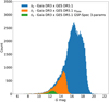 |
Fig. 1 Distributions of the G magnitudes of the GES parent sample (𝒮0; blue), of the GES stars having a Gaia DR3 radial velocity (𝒮1; orange), and of the Gaia-ESO stars having the three main Gaia GSP-Spec atmospheric parameters (𝒮3; green). The bin positions and width are identical for the three histograms; the bin width was adjusted using the Freedman-Diaconis rule. |
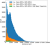 |
Fig. 2 Distributions of the Gaia distances (Bayesian distances from Bailer-Jones et al. 2021) of the of the GES parent sample (𝒮0; blue), of the stars having a Gaia DR3 radial velocity (𝒮1; orange), and of the stars having the three main Gaia GSP-Spec atmospheric parameters (𝒮3; green). The bin positions and width are identical for the three histograms; the bin width was adjusted using the Freedman-Diaconis rule. |
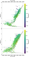 |
Fig. 3 Kiel diagram of the 2079 stars in the subsample 𝒮3, colour-coded by metallicity. A grid of Parsec isochrones (Bressan et al. 2012) with solar metallicity and ages ranging from 0.1 to 14 Gy is superimposed. Top panel: based on the Gaia-ESO atmospheric parameters; bottom panel: based on the uncalibrated Gaia GSP-Spec atmospheric parameters. |
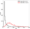 |
Fig. 4 Distributions of the GES (red) and Gaia RVS (black) S/N for 1117 stars having both values. |
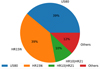 |
Fig. 5 Pie chart of the distribution of the 2079 stars of the subsample 𝒮3 according to the GES setup used to derive the GES recommended atmospheric parameters. |
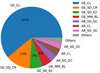 |
Fig. 6 Pie chart of the distribution of the 2079 stars of the subsample 𝒮3 according to their GES field type. |
3 Radial velocities and detection of non-single stars
3.1 Comparison between Gaia and GES radial velocities
In this section, we compare the radial velocities of the stars in the sample 𝒮1. We discard the following stars: a) those flagged as SBn ≥ 1 in Gaia-ESO and as non-single star in Gaia since their radial velocities are likely time-dependent; b) those having the GES simplified flags SRP (data-reduction problems) or SRV (suspicious radial velocities) or EML (emission lines) since it may indicate a less precise or less accurate radial velocity; c) those having RUWE ≥ 1.4 since it may indicate a suspicious Gaia astrometric solution; d) those having the Gaia phot_variable_flag set to True. After this cleaning, the sample 𝒮1 is downsized to 14 692 objects.
Figure 7 shows the distribution of the radial velocity differences υrad,Gaia − υrad,GES normalised by the propagated errors ![$\[\sqrt{\sigma\left[v_{\text {rad,Gaia }}\right]^2+\sigma\left[v_{\text {rad,GES }}\right]^2}\]$](/articles/aa/full_html/2024/10/aa50357-24/aa50357-24-eq1.png) (sample histogram and sample KDE) and for reference, it also displays the normal law 𝒩 (0, 1). If we assume that for a given star, each Gaia (GES, respectively) radial velocity is a random variable distributed along a normal law 𝒩 (υrad, σ[υrad]2) where υrad is the true radial velocity of the star and σ[υrad] describes the instrumental error, then υrad,Gaia − υrad,GES should follow a probability distribution 𝒩(0, σ[υrad,Gaia]2 + σ[υrad,GES]2), or equivalently, the normalised differences
(sample histogram and sample KDE) and for reference, it also displays the normal law 𝒩 (0, 1). If we assume that for a given star, each Gaia (GES, respectively) radial velocity is a random variable distributed along a normal law 𝒩 (υrad, σ[υrad]2) where υrad is the true radial velocity of the star and σ[υrad] describes the instrumental error, then υrad,Gaia − υrad,GES should follow a probability distribution 𝒩(0, σ[υrad,Gaia]2 + σ[υrad,GES]2), or equivalently, the normalised differences ![$\[\Delta_{\text {norm }} v_{\text {rad }}=\left(v_{\mathrm{rad}, \mathrm{Gaia}}-v_{\mathrm{rad}, \mathrm{GES}}\right) / \sqrt{\sigma\left[v_{\mathrm{rad}, \mathrm{Gaia}}\right]^2+\sigma\left[v_{\mathrm{rad}, \mathrm{GES}}\right]^2}\]$](/articles/aa/full_html/2024/10/aa50357-24/aa50357-24-eq2.png) should follow a probability distribution 𝒩 (0, 1).
should follow a probability distribution 𝒩 (0, 1).
The mean of Δnormυrad is −0.03 and its standard deviation is 1.68. Fig. 7 shows that the sample probability distribution deviates marginally from the normal law: while the core of the sample distribution follows closely the normal law, we note that the tails of the sample distribution for |ΔnormV| ⪆ 2.3 (the approximate abscissa where the left and right sample tails are above the normal law) are heavier than those of the normal law. The sample left and right tails are populated by 999 (≈6.8%) objects and about 580 objects are likely in excess compared to the normal law. For those 580 objects (≈4% of the sample), the random uncertainty reported by the two experiment is not able to explain the radial velocity differences between the Gaia and GES datasets. This could be due to an incorrect estimate of the random uncertainty (e.g., see Jackson et al. 2015 for a discussion on the non-Gaussianity of the random uncertainty in GES) or a biased estimate of υrad. It could also be due to a still unidentified astrophysical variation (e.g. stellar multiplicity, jitter, pulsations) of the radial velocity.
The statistical difference between the two sets of 14692 radial velocities can also be evaluated with a two-sample K-S test. Computed with the SCIPY module, for υrad,GES and υrad,Gaia, the test returns a statistics D = 0.004 and a p-value of 0.999 under the null hypothesis H0: “the two samples are drawn from the same unknown distribution”. Therefore, we fail at rejecting the null hypothesis at the confidence level α = 0.05: in other words, there is no strong evidence that the two datasets are statistically different. This result is in agreement with the discussion of the previous paragraph.
We remind the reader that Gaia-ESO has observed their targets with a various choice of FLAMES/UVES and FLAMES/GIRAFFE setups, meaning that two given stars are not necessarily observed with the same setup, and so they are not observed at the same wavelengths and same resolution. During the homogenisation phase, Gaia-ESO has selected the single setup or the combination of setups that will be used to publish the final (average) radial velocity of a given star. This choice can be traced back using the column ORIGIN_VRAD of the GES catalogue. The setup HR10 was used as a reference setup by Gaia-ESO and velocity offsets have been computed and applied to put the radial velocities measured from other setups onto the HR10 radial velocity scale. A consequence of this observational strategy is that the agreement between the GES and Gaia radial velocities may vary between setups (e.g. quality of the wavelength calibration of a given setup, efficiency of the cross-correlation technique depending on the absorption-line content of a given setup). Table 1 lists the mean, median and standard deviation of ![$\[\Delta_{\text {norm }} v_{\text {rad }}=\left(v_{\mathrm{rad}, \mathrm{Gaia}}-v_{\mathrm{rad}, \mathrm{GES}}\right) / \sqrt{\sigma\left[v_{\mathrm{rad}, \mathrm{Gaia}}\right]^2+\sigma\left[v_{\mathrm{rad}, \mathrm{GES}}\right]^2}\]$](/articles/aa/full_html/2024/10/aa50357-24/aa50357-24-eq6.png) and of
and of ![$\[\Delta v_{\mathrm{rad}}=v_{\text {rad,Gaia }}-v_{\text {rad,GES }}\]$](/articles/aa/full_html/2024/10/aa50357-24/aa50357-24-eq7.png) when only one GES-setup combination is used for the Gaia vs. GES comparison. We note that indeed, the agreement between the GES and Gaia radial velocity scales depends on the GES setup. An excellent agreement is obtained when the GES radial velocity derives from observations with HR10, HR15N, HR3, U580: the mean of Δnormυrad is below 0.1 in absolute value and its standard deviation is below 2. For three setups (HR9B, HR14A, U520) used for warm stars, the standard deviation of Δnormυrad is larger than 3 and the mean of Δnormυrad is larger than ≈0.2 in absolute value. This larger bias and larger scatter of Δnormυrad for these three setups are not correlated with the mean G magnitude nor the mean Teff,GES of the stars nor the mean S/N of GES spectra. According to the last column ‘STD’ of Table 3 in Hourihane et al. (2023), the radial velocity homogenisation was less precise for HR9B, HR14A and U520 than for HR15N, HR21, U580 but it was not worse than for HR3 and WG13 combination.
when only one GES-setup combination is used for the Gaia vs. GES comparison. We note that indeed, the agreement between the GES and Gaia radial velocity scales depends on the GES setup. An excellent agreement is obtained when the GES radial velocity derives from observations with HR10, HR15N, HR3, U580: the mean of Δnormυrad is below 0.1 in absolute value and its standard deviation is below 2. For three setups (HR9B, HR14A, U520) used for warm stars, the standard deviation of Δnormυrad is larger than 3 and the mean of Δnormυrad is larger than ≈0.2 in absolute value. This larger bias and larger scatter of Δnormυrad for these three setups are not correlated with the mean G magnitude nor the mean Teff,GES of the stars nor the mean S/N of GES spectra. According to the last column ‘STD’ of Table 3 in Hourihane et al. (2023), the radial velocity homogenisation was less precise for HR9B, HR14A and U520 than for HR15N, HR21, U580 but it was not worse than for HR3 and WG13 combination.
Figure 8 shows the dependency of Δnormυrad with G magnitude, Teff,ges, log gGES and [Fe/H]GES. We note that the distributions are rather symmetrical around Δnormυrad = 0: the difference between the GES and Gaia radial velocities is not correlated with any of these four parameters. As a last remark, we note that Katz et al. (2023) recommend a correction of the Gaia radial velocity in the form of calibration depending on GRVS. If we apply it, the correction is never larger than 0.4 km s−1, the sample is downsized to 14173 objects because of some unavailable GRVS estimates; the mean of Δnormυrad becomes −0.09 and its standard deviation remains unchanged at 1.67. The rest of the discussion remains true. We also note that Babusiaux et al. (2023) show that the uncertainty on the Gaia radial velocity is underestimated. They publish a calibration as a function of GRVS to estimate a correcting factor. There calibration seems to be defined only on the GRVS range [8, 14; we cannot compute the correcting factor for a small fraction of our selection brighter than GRVS = 8. Taking into account this correction does not change the above discussion. Figure A.1 is the same as Fig. 7 but it uses the corrected uncertainties for Gaia radial velocities instead of the raw ones.
In conclusion, after discarding objects with suspicious or variable radial velocities from the sample 𝒮1, we find an excellent agreement between the GES and Gaia radial velocity scales, given their respective uncertainties. The mean and median difference between the two datasets are respectively 0.07 and −0.02 km s−1. We cannot explain the disagreement for about 4% of the analysed stars.
Mean, median and standard deviation of ![$\[\Delta_{\text {norm }} v_{\text {rad }}=\left(v_{\text {rad,Gaia }}-v_{\text {rad,GES }}\right) / \sqrt{\sigma\left[v_{\text {rad,Gaia }}\right]^2+\sigma\left[v_{\mathrm{rad}, \mathrm{GES}}\right]^2}\]$](/articles/aa/full_html/2024/10/aa50357-24/aa50357-24-eq3.png) and υrad = υrad,Gaia − υrad,GES when only one GES-setup combination is used for the comparison.
and υrad = υrad,Gaia − υrad,GES when only one GES-setup combination is used for the comparison.
 |
Fig. 7 Probability distribution of the normalised velocity differences. The blue histogram (bin width = 0.1) displays the distribution Δnormυrad of the difference of the radial velocity differences υrad,Gaia − υrad,GES normalised by the propagated errors |
![$\[\sqrt{\sigma\left[v_{\mathrm{rad}, \mathrm{Gaia}}\right]^2+\sigma\left[v_{\mathrm{rad}, \mathrm{GES}}\right]^2}\]$](/articles/aa/full_html/2024/10/aa50357-24/aa50357-24-eq5.png)
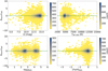 |
Fig. 8 From top to bottom, left to right: Δnormυrad vs. G magnitude, Teff,GES, log gGES and [Fe/H]GES. The vertical axis is the same for the four panels. The colour scale changes from one plot to another. |
3.2 Binarity
The Gaia-ESO is not designed to discover and monitor the variations of the radial velocities of a star with time. Nonetheless, thanks to the repeated observations needed to achieve a S/N sufficient for determining abundances, and thanks to the good resolving power of the FLAMES/GIRAFFE and FLAMES/UVES multi-object spectrographs, it is still possible to identify spectroscopic binaries with one visible component (SB1), discovered by looking for unaccountably scattered radial velocity series, and spectroscopic binaries with two or more visible components (SBn ≥ 2), discovered by finding multi-peaked cross-correlation functions (CCFs).
A final census of the GES SB1 and SBn ≥ 2, based on the analysis of the final data release, is still under preparation (Van der Swaelmen et al., in prep.): our preliminary analysis of GES DR5.1 give a total of 2117 SBn with 1216 SB1, 878 SB2, 20 SB3 and three SB4. However, three publications have made use of the previous internal GES data releases. Merle et al. (2017) have listed 342 SB2, 11 SB3 and one SB4 after analysing the whole GES iDR4; Merle et al. (2020) have found 803 SB1 among the HR10 and HR21 observations released in GES iDR5; finally, Van der Swaelmen et al. (2023) have found 322 SB2 (four of which being also SB3 candidates), ten SB3 and two SB4 among the HR10 and HR21 observations of field stars released in GES iDR5. Once combined, these three publications give a list of 1113 unique SBn. Merle et al. (2017) used the CCFs computed by the GES WG, while Merle et al. (2020) and Van der Swaelmen et al. (2023) are using the Nacre CCFs described and computed in Van der Swaelmen et al. (2023). A future publication will exploit the strength of the Nacre CCFs to provide the complete census of GES SB1 and SBn ≥ 2 among the GIRAFFE (HR10, HR21 and HR15N) and UVES observations but in the mean time, it is still possible to check how the GES SBs are flagged by Gaia. We point the reader that a detailed comparison of GES iDR5 and Gaia DR3 in terms of binarity is given in Van der Swaelmen et al. (2023).
Gaia DR3 provides various ways to identify confirmed or suspected non-single stars. The most direct way is to look at the column non_single_star of the Gaia main catalogue to find the confirmed stellar multiples. Due to stringent filters, the Gaia DR3 multiple-star census is mostly populated by bright object (G ≤ 13) and therefore, one can anticipate a small intersection with the GES multiple-star census. Using the published (resp., new preliminary) census, we found 8 out of 1113 (resp., 22 out of 2117) SBn among GES DR5.1 targets that are also flagged as non-single stars by Gaia DR3: two (resp., 12) astrometric binaries, one (resp., two) eclipsing binaries, five (resp., eight) spectroscopic binaries and zero binaries confirmed by a combination of techniques. 161 (resp., 414) GES SBn have a Gaia radial velocity. The median uncertainty on the Gaia radial velocity is slightly larger for the GES SBn than for the non-SBn: 3.91 km s−1 vs. 3.24 km s−1 (resp., 4.26 km s−1 vs. 3.22 km s−1). In other words, the uncertainty on the Gaia radial velocity tends to be slightly larger for the population of GES SBn candidates. The fact that the GES SBn population has a larger median uncertainty on their Gaia radial velocity may indicate that, in future Gaia releases, these faint objects will also be seen as non-single stars by Gaia.
The quantity RUWE (Renormalised Unit Weight Error) can be used to identify objects for which the single-star model does not permit a good fit of the astrometric observations. The Gaia documentation indicates that a RUWE larger than 1.4 should be treated as unusual and this may or may not point at a hidden stellar companion. 7440 objects of 𝒮0 have RUWE ≥ 1.4 but only 66 (resp., 168) are flagged has SBn in the published (resp., preliminary) GES census: we confirm that RUWE ≥ 1.4 is not a necessary nor a sufficient condition to identify spectroscopic binaries.
The Gaia ‘Astrophysical parameters’ tables provide the community with a series of columns that are intended to help in tracking down potential binaries. Van der Swaelmen et al. (2023) discuss the use of the columns classprob_dsc_combmod_binarystar and classprob_dsc_specmod_binarystar from the Discrete Source Classifier (DSC; Delchambre et al. 2023) and flags_msc from the Multiple Star Classifier (MSC; Creevey et al. 2023). We find zero (resp., six and five for the preliminary final census) GES SB2 with a probability classprob_dsc_combmod_binarystar and classprob_dsc_specmod_binarystar larger than 0.5. Among the preliminary census, there are six and two GES SB2 with a probability classprob_dsc_combmod_binarystar and classprob_dsc_specmod_binarystar larger than 0.9. According to Delchambre et al. (2023), only 0.2% of the unresolved binaries of their validation data-set are recovered (see their Table 3) by the two DSC classifiers. Therefore, we do not expect more than a couple SB2 to be correctly flagged by DSC: our findings seem to be compatible with their prediction: 303 (resp., 748) GES SB2 have flags_msc set to 0, which indicate that the inference of atmospheric parameters of each component cannot be rejected a priori.
4 Rotational velocities
In this section, we compare the projected rotational velocity υ sin iges and the broadening parameter υbroad,Gaia (Frémat et al. 2023) for the 2094 stars of the sample 𝒮2. Gaia-ESO provides no estimate of υ sin i for 262 out of 2094 stars with a valid υbroad,Gaia. The sample S2 is therefore downsized to 1832 objects. Figure 9 shows the (normalised) distributions of υ sin iGES and υbroad,Gaia. We note that the two distributions are quite different: the mode and median of the distribution of Gaia-ESO υ sin i are about 8 km s−1, while the mode and median of the distribution of υbroad,Gaia are around 11 km s−1. It is expected since υ sin iGES and υbroad,Gaia do not measure the same quantity. The Gaia-ESO quantity named υ sin i in the final public release comes from one of three possible sources according to Hourihane et al. (2023): the global fitting code ROTFIT by the OACT node for GIRAFFE spectra (e.g. Frasca et al. 2015), the CCF width − υ sin i calibration by the Arcetri node for UVES spectra (Sacco et al. 2014) and one estimate or a combination of estimates provided by the WG13 for stars in young clusters. All the used techniques account for the GIRAFFE or UVES instrumental resolution such that υ sin iGES takes into account the spectral broadening due to the stellar rotation and the macroturbulence. On the other hand, for Gaia RVS, υbroad,Gaia measures any source of broadening: instrumental, rotation, turbulence. We therefore do not expect a strong correlation between these two parameters: indeed, the linear regression shown in Fig. 10 gives a slope of 0.796 ± 0.011, a y-intercept of 5.559 ± 0.571 and the coefficient r2 = 0.72495 indicates a loose correlation. This selection is essentially FGK dwarf and giant stars with a G magnitude in the range [10, 14]: such stars have in general a small rotational velocity that causes a line-broadening smaller or comparable to the one caused by the instrumental resolution. In their Table 3, Frémat et al. (2023) give a υbroad,Gaia range as a function of G and Teff where υbroad,Gaia has a probability higher than 90% to be within 2σ of υυ sin i. For FGK stars (Teff = 4000 K or 5500 K or 7500 K in their table) and for G ≥ 10, the validity range is for υbroad,Gaia ⪆ 12 km s−1 (conservative value). If we restrict the sample to stars fainter than G = 10 and with υbroad,Gaia ⪆ 12 km s−1, the correlation coefficient r2 marginally increases and remains below 0.8, still indicating a loose correlation. In other words, υbroad,Gaia is not a reliable proxy for υ sin iGES, especially for slow rotators. Our results are compatible with the results obtained by Frémat et al. (2023) when they compare the Gaia broadening parameter to the rotational velocities published by APOGEE and GALAH (and also, by RAVE and LAMOST, but the resolution of these two surveys is much lower than those of Gaia-ESO).
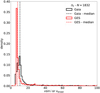 |
Fig. 9 Normalised histogram of υ sin iGES (red) and the broadening parameter υbroad,Gaia (black). |
Summary of the star selection.
5 Temperatures, gravities and abundances
In this section, we compare the spectroscopic parameters of the stars in common between the two surveys for the 2079 stars of the sample 𝒮3. As stated in Sec. 2.3, the initial selection 𝒮3 of 2079 stars is obtained by requesting the availability of the three Gaia GSP-Spec parameters {Teff, log g, [Fe/H]} for a star of the parent sample. Then, we check in the GES DR5.1 catalogue if some stellar parameters and some abundances have been derived by the GES consortium. The result of such counting is summarised in the Table 2. We note that some of the stars of 𝒮3 are missing the corresponding GES stellar parameters. Thus, 1939 stars have both Gaia GSP-Spec and GES Teff, 1575 stars both Gaia GSP-Spec and GES log g, and 1904 stars both Gaia GSP-Spec and GES [Fe/H]. Table 2 also counts the published abundances in GES and Gaia for the stars in 𝒮3. As expected, this time, the GES catalogue is more complete than the Gaia DR3 catalogue when it comes to individual abundances. Four α elements – namely Mg, Si, Ca, and Ti – possess individual abundances in both Gaia DR3 and Gaia-ESO DR5.1 for more than 100 stars. Since the Gaia RVS spectra are centred around the strong lines of the near-infrared Ca II triplet, Ca is logically the element most-often measured by Gaia GSP-Spec and 503 stars have a Ca abundance in both surveys. In the next subsections, we present statistical tests done on the atmospheric parameters and abundances of the selected stars to discuss the agreement between the GES and Gaia catalogues.
Recio-Blanco et al. (2023) use three external heterogeneous (different instruments, spectral coverage, analysis methods) catalogues, namely APOGEE DR17, GALAH DR3 and RAVE DR6, to validate the GSP-Spec parametrisation of the Gaia RVS spectra. In short, after filtering using the uncertainties and quality flags provided in these external catalogues and the GSP-Spec flags, Recio-Blanco et al. (2023) define a best-quality subset (170000 unique stars) and a medium-quality subset (750000 unique stars) to investigate the possible differences between the GSP-Spec parameters ({Teff, log g, [M/H]}) and the literature-compilation ones. The authors find no biases for Teff but provide the reader with three calibrations in the form of low-order (n ≤ 4) polynomials to correct for the identified biases for log g and [M/H]: a calibration for log g (hereafter, ‘calibrated log g′), a general calibration for [M/H] (hereafter, ‘calibrated [M/H]’) and a specific calibration for [M/H] in open clusters (hereafter, ‘OC-calibrated [M/H]’). The authors check also the dependency of individual abundances with the surface gravity using a subset of GSP-Spec-parametrised Gaia sources. A series of calibrations for the GSP-Spec abundance ratios are derived by forcing stars of the solar neighbourhood with near-solar metallicities and on near-circular orbits to have [X/Fe] close to zero. It is worth noting here that a) the aforementioned calibrations are not guaranteed to work for any science case or for any volume of the parameter space; b) GSP-Spec atmospheric parameters are calibrated against external catalogues while GSP-Spec individual abundances are calibrated against a subset of the GSP-Spec catalogue; c) since each spectroscopic survey comes with its own biases induced by the choice of analysis techniques and tools, the need for recalibrating the GSP-Spec parameters is to be expected. Recio-Blanco et al. (2023) publish also a set of quality flags for the atmospheric parameters and the chemical abundances. Out of the thirteen flags qualifying the atmospheric parameters and for the 2079 stars of the sample 𝒮2, all are set to 0 except for the flag fluxNoise (flag07): for 889 stars, fluxNoise is set to 0; for 809 stars, it is set to 1; for 324 stars, it is set to 2; for 57 stars, it is set to 3. The present study is interesting in that it will independently test the recommended GSP-Spec calibrations and quality flags against another external catalogue not really used by Recio-Blanco et al. (2023) in their validation, namely GES DR5.1, and furthermore, these tests are carried out in the faint-magnitude regime.
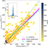 |
Fig. 10 υbroad,Gaia vs υ sin iGES (2D histogram). The green dashed line is the 1-to-1 relation. The pink thick line is the linear regression (see text for the parametrisation). The cyan thick dashed line is a non-parametric LOWESS model (locally weighted linear regression) implemented using the Python module StatsModels. The inset shows the distribution of Δυbroad = υbroad,Gaia − υ sin iGES. The red dashed line in the inset indicates the location of the mean difference. |
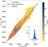 |
Fig. 11 Comparison of the effective temperatures for the 1939 stars of 𝒮3 with both a Gaia GSP-Spec and GES temperature estimate. The 2D hexagonal bins are colour-coded by the number of stars. The red lines show density levels containing 68, 80, 90 and 95% of the population. The dashed green line shows the 1-to-1 relation, the pink thick line is the linear regression (see text for the parametrisation). The cyan thick dashed line is the LOWESS line. The inset shows the distribution of Δeff = Teff,Gaia − Teff,GES. |
5.1 Effective temperature
In Figure 11, we show the comparison between the effective temperatures for 1939 stars of the subsample 𝒮3. The distribution lies along the 1-to-l relation and the linear regression give a slope of 0.975 ± 0.007, a y-intercept of 210 K ± 32 K and a coefficient r2 = 0.921. We conclude that Teff,GES and Teff,Gaia are strongly correlated. Figure 12 shows the empirical cumulated distribution functions (ECDF) and the D-statistic of the two-sample Kolmogorov-Smirnov (KS) test. We find D = 0.1367 and a p-value of 3 × 10⁻¹⁶, which indicates that we should reject the null hypothesis that the two distributions are drawn from the same distribution: it is not surprising given the degeneracies that hamper the determination of atmospheric parameters and the different methods adopted by Gaia-ESO and GSP-Spec to get these parameters. We find a mean and standard deviation for ΔTeff = Teff,Gaia − Teff,GES of 89 K and 170 K. Allowing only fluxNoise = 0 or 1 does not significantly change the comparison. If we keep only the objects with fluxNoise set to 0, the mean and standard deviation become 38 K and 112 K, but the sample size is divided by more than two (829 objects left).
5.2 Surface gravity
In Figure 13, we compare the GES surface gravity log g of 1575 stars to the Gaia uncalibrated (top panel) and calibrated (bottom panel) log g. We find a mean and standard deviation for Δ log g = log gGaia,uncal − log gGES of −0.19 and 0.39, indicating that log gGaia,uncal is underestimated on average. The behaviour is slightly different if we split the population in dwarf and giant stars: the mean and standard deviation become −0.09 and 0.30 for dwarf stars (329 objects with log gGES ≥ 3.5), and − 0. 22 and 0. 40 for giant stars (1246 objects). The bias affecting log gGaia,uncal is a bit larger, in absolute value, for the giant subpopulation than for the dwarf subsample.
The GSP-Spec calibrated gravity improves the situation for both dwarf and giant stars. For the full sample, the mean and standard deviation for Δ log g = log gGaia.cal − log gGES become 0.08 and 0.37, respectively; for the dwarf subsample, they are equal to −0.03 and 0.26, respectively; for the giant subsample, they are equal to 0.11 and 0.37, respectively. The parameters (slope, y-intercept and r2) of the linear regressions shown in Fig. 13 are: (0.998, −0.185, 0.8161) for the log gGaia,uncal and (0.866, 0.455, 0.8137) for log gGaia,cal. If we keep only the objects with fluxNoise set to 0, the mean and standard deviation become −0.02 and 0.28, but again the sample size is divided by more than two (710 objects left). We conclude that it is better to use the calibrated GSP-Spec gravity and to clean the selection with the help of the quality flags, in line with the prescriptions from Recio-Blanco et al. (2023).
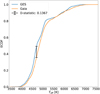 |
Fig. 12 Empirical cumulative distribution function (ECDF; continuous line) and D-statistic (vertical line) of the two-sample KS test for Teff,GES (blue) and Teff,GES (orange). |
5.3 Metallicity
In this section, we compare the 1904 objects with both a GES and a Gaia [Fe/H] estimates. Figure 14 shows the comparison for the uncalibrated, the calibrated and the OC-calibrated Gaia [M/H]. The metallicity range goes from −2.2 dex to 0.5 dex in terms of GES [Fe/H] but 94% of the 1904 stars have a [Fe/H]GES in [−0.5, 0.5]. The mean and standard deviation of Δ[Fe/H] = [Fe/H]Gaia − [Fe/H]GES are: 0.03 dex and 0.17 dex for the uncalibrated metallicity, 0.03 dex and 0.16 dex for the calibrated metallicity, and 0.02 dex and 0.16 dex for the OC-calibrated metallicity. The parameters (slope, y-intercept, r2) of the linear regressions are: (0.887, 0.020, 0.6744) for the uncalibrated metallicity, (0.855, 0.014, 0.6896) for the calibrated metallicity, (0.835, 0.008, 0.6759) for the OC-calibrated metallicity. If we keep only the objects with fluxNoise set to 0, the mean and standard deviation become −0.03 and 0.13 for the uncalibrated case, and −0.01 and 0.12 for the calibrated case, but again the sample size is divided by more than two (822 objects left). We conclude from these comparisons that the two calibrations and a flag-based selection appear to marginally improve the agreement between the GES and the Gaia metallicity scales, in agreement with Section 4.3 of Babusiaux et al. (2023).
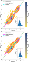 |
Fig. 13 Comparison of the Gaia-ESO surface gravity with that of Gaia uncalibrated (top) and calibrated (bottom) ones. Symbols and colours are as in the Fig. 11. |
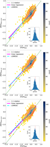 |
Fig. 14 Comparison of the Gaia-ESO metallicity with that of Gaia uncalibrated (top), calibrated (middle) and OC-calibrated (bottom) ones. Symbols and colours are as in the Fig. 11. |
5.4 α abundance
We now compare the 1037 objects of S3 with a valid measurement of the α content in the GES DR5.1 and the Gaia DR3 catalogues. For Gaia-ESO, [α/Fe] is obtained by averaging the abundances of Mg, Si, Ca and Ti; for Gaia, [α/Fe] is directly parametrised. Figure 15 shows the comparison between GES and Gaia for the GSP-Spec uncalibrated, calibrated, Teff-calibrated and log g-calibrated values. The sample is made of Milky Way disc stars and therefore, [α/Fe] approximately ranges from 0 to 0.4 in terms of GES [α/Fe]. The mean and standard deviation of Δ[α/Fe] = [α/Fe]Gaia − [α/Fe]GES are: −0.06 dex and 0.14 dex for the uncalibrated [α/Fe], −0.05 dex and 0.13 dex for the calibrated [α/Fe], −0.09 dex and 0.13 dex for the Teff-calibrated [α/Fe], and −0.04 dex and 0.12 dex for the log g-calibrated [α/Fe]. Imposing fluxNoise equal to 0 does not significantly improve the agreement. For instance, the mean and standard deviation become −0.05 dex and 0.11 dex for the calibrated case. These numbers indicate that the calibrated [α/Fe] and log g-calibrated [α/Fe] and the use of the quality flags, though preferable, offer a marginal improvement for the sample under study. It is in agreement with Babusiaux et al. (2023) who note that biases remain after applying one of the above calibrations for [α/Fe].
In late-type stars, the RVS spectrum will be dominated by the Ca II triplet lines, and therefore, calcium will weigh more in the estimation of the Gaia [α/Fe] parameter. Figure 16 compares the Gaia [α/Fe] to the GES [Ca/Fe]. The mean and standard deviation of Δ[α/Fe] = [α/Fe]Gaia [Ca/Fe]GES are: 0.03 dex and 0.16 dex for the uncalibrated [α/Fe], 0.04 dex and 0.16 dex for the calibrated [α/Fe], 0 dex and 0.16 dex for the Teff-calibrated [α/Fe], and 0.05 dex and 0.16 dex for the log g-calibrated [α/Fe]. The plots and these numbers show that there is indeed a similar agreement between GES [Ca/Fe] and Gaia [α/Fe] as there is between GES [α/Fe] and Gaia [α/Fe]. In other words, for the sample under study, the agreement between Gaia [α/Fe] and the GES [Ca/Fe] is as good as the agreement between Gaia [α/Fe] and the GES [α/Fe].
5.5 Individual abundances
In Figures 17 and 18, we compare [X/Fe] for seven of the eight elements available both in GES and Gaia: four α elements (Mg, Si, Ca, Ti), two iron peak elements (Cr and Ni) and one neutron-capture element (Ce). We note that the GES-Gaia intersection leads to small to very small samples (fewer than 20 data points for Cr and Ce) when it comes to comparing individual abundances. Nevertheless, Figures 17 and 18 suggests that the best agreement is obtained for Ca, Ti and Ni (smallest biases) and the agreement is a bit worse for Mg and Si. We cannot conclude for Cr and Ce because of the paucity of data. For Mg, Si, Ti and Ni, we note that the GSP-Spec quality flags take either the values 0, 1 or 2 (rarely for Si and Ti). For Ca, all of the 503 stars have their Ca abundance quality flags set to 0. In particular, for these five species, none of the stars has an abundance quality flag set to 9, i.e. a value that should be absolutely discarded according to the prescriptions from Recio-Blanco et al. (2023).
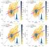 |
Fig. 15 Comparison of the Gaia-ESO [α/Fe] with that of Gaia uncalibrated (top left), calibrated (top right), Teff-calibrated (bottom left) and log g-calibrated (bottom right) ones. Symbols and colours are as in the Fig. 11. |
5.6 Dependency with G magnitude
Figure 19 investigates the dependency of the difference between Gaia and Gaia-ESO parameters Δ𝒫 = 𝒫Gaia − 𝒫GES as a function of the G magnitude where 𝒫 is Teff, log g (log gGaia,uncal or log gGaia,cal for GSP-Spec), [Fe/H] ([M/H]Gaia or [M/H]Gaia,cal for GSP-Spec) or [Ca/Fe]. Table 3 gives the mean and standard deviation of Δ𝒫 for two G-magnitude ranges [3.47, 11[ and [11, 13.87] as well as the p-value of the Kolmogorov-Smirnov two-sample test for these two subsamples. Table 3 also investigates different selections based on the setup used in Gaia-ESO to observe a given star (high resolution UVES U580 vs. medium resolution GIRAFFE HR15N) or the evolutionary stage of a given star (dwarf vs. giant).
As already noted in Figure 1, faint objects are more numerous than bright objects in our sample: 91% (1885/2079) of the Gaia – GES subset intersection lie in the G range [11, 13.87]. This is a consequence of the GES selection function: Gaia-ESO is indeed designed to sample the faint part of the Gaia catalogue and 79% of the full GES DR5.1 catalogue has a G magnitude bigger than 15. For the full intersection 𝒮3, we note that for the temperature, surface gravity and metallicity, the two subsamples obtained for G < 11 mag and G ≥ 11 mag behave differently: a) the mean and standard deviation of the ΔTeff, Δ log g and Δ[Fe/H] increase with G (so when stars get fainter); b) often, the p-values are extremely small indicating that we can reject the null hypothesis that the two subsamples are drawn from the same underlying distribution. As already noted in the previous subsections, the use of the GSP-Spec calibrated gravity instead of the uncalibrated gravity allows us to get the centre of the distribution closer to the line Δ log g = 0 but a small offset of 0.08 still exists and the difference between the mean Δ log g of the bright and the faint subsamples remains 0.15 in absolute value. The same behaviour is observed when we breaks the initial Gaia – GES intersection according to the GES setup (U580 or HR15N) or the evolutionary stage (dwarf vs. giant). An exception may exist for the gravity in the case of dwarf stars: the different behaviour between the bright and the faint subsamples tends to vanish, in particular when we use the calibrated gravity. One knows that the determination of the atmospheric parameters is a degenerate problem, and indeed, we observe positive correlations between two Δ𝒫 as shown in Fig. 20: in other words, Teff, log g and [Fe/H] tend to be simultaneously overestimated.
On the other hand, Δ [Ca/Fe] shows little dependency with G: the distribution is flat around Δ[Ca/Fe] ≈ 0.05 and we cannot reject the null hypothesis that the two subsamples corresponding to the bright and the faint ranges are drawn from the same underlying distribution. These remarks hold when we break the full intersection according to the GES setups or the stellar evolutionary stage. This is a frequent observation in stellar spectroscopic studies where systematic effects tend to cancel out for abundance ratios in the form [X/Fe]. Indeed, we do not find a correlation between ΔTeff and Δ [Ca/Fe] or between Δ log g and Δ[Ca/Fe].
The cut at G ≈ 11 mag adopted above is empirically chosen from the plots in Fig. 19: one could argue that the bright sample covers about seven magnitudes, while the faint sample covers only three magnitudes, and that the number of data-points is significantly different between the two magnitude ranges. However, we see that this bifurcation around G ≈ 11 mag is seen in Fig. 21 displaying the change of the error on a given GSP-Spec parameter e (𝒫Gaia) as a function of the G magnitude. Since GSP-Spec gives for each quantity a lower and upper uncertainty, not necessarily symmetrical, we define e (𝒫Gaia) as the arithmetic average of the lower and upper uncertainties. The Figure 21 relies only on Gaia data and does not include GES data. It shows clearly that a change happens around G ⪆ 11 mag: e(𝒫Gaia) becomes significantly scattered for G ⪆ 11 mag compared to its typical scatter for G ⪅ 11 mag.
Unsurprisingly, as shown in Fig. 22, the G magnitude and the Gaia RVS S/N is strongly correlated. More specifically, G and log SNRRVS are linearly dependent. On the other hand, the relation between the G magnitude and the GES S/N is not straightforward since, within Gaia-ESO, the exposure time has been adjusted depending on the magnitude regime in which the target lies; still, the GES S/N tends to be higher towards lower G mag. If we combine the two S/N through, for instance, a geometric mean ![$\[\sqrt{\mathrm{SNR}_{\mathrm{GES}} \mathrm{SNR}_{\mathrm{RVS}}}\]$](/articles/aa/full_html/2024/10/aa50357-24/aa50357-24-eq8.png) , the correlation between the two quantity remains tight: the logarithm of the geometric average of the two S/N approximately varies linearly with G (based on only 552 objects of 𝒮3 with published S/N for the RVS spectra). No sharp drop of the S/N is to be noted at G ≈ 11 mag, it still follows the relation observed at brighter regime. However, the mean RVS S/N is 83 in the G range [10, 11], 51 in the G range [11, 12] and 29 in the G range [12, 14]. While a S/N of 30 is still enough in high-resolution spectroscopy of faint objects to estimate parameters with, for example, typical uncertainties lower than 150 K for Teff or lower than 0.15 dex for the α abundances, it appears that at the RVS resolution and sampling, and for the RVS wavelength window, a S/N lower than ≈50–70 is not enough to reach such a precision for faint objects. Finally, we note that the GSP-Spec flags flag01 to flag13 but not flag07 are equal to 0 for all of the 2079 stars in the Gaia – GES intersection. The flag 7 can be equal to 0, 1, 2 or 3 but forcing flag07 to be equal to 0 does not make the scatter of Δ𝒫 for the faint range similar to that of the bright range.
, the correlation between the two quantity remains tight: the logarithm of the geometric average of the two S/N approximately varies linearly with G (based on only 552 objects of 𝒮3 with published S/N for the RVS spectra). No sharp drop of the S/N is to be noted at G ≈ 11 mag, it still follows the relation observed at brighter regime. However, the mean RVS S/N is 83 in the G range [10, 11], 51 in the G range [11, 12] and 29 in the G range [12, 14]. While a S/N of 30 is still enough in high-resolution spectroscopy of faint objects to estimate parameters with, for example, typical uncertainties lower than 150 K for Teff or lower than 0.15 dex for the α abundances, it appears that at the RVS resolution and sampling, and for the RVS wavelength window, a S/N lower than ≈50–70 is not enough to reach such a precision for faint objects. Finally, we note that the GSP-Spec flags flag01 to flag13 but not flag07 are equal to 0 for all of the 2079 stars in the Gaia – GES intersection. The flag 7 can be equal to 0, 1, 2 or 3 but forcing flag07 to be equal to 0 does not make the scatter of Δ𝒫 for the faint range similar to that of the bright range.
It would be more homogeneous to compare the spectroscopic quantities to GRVS instead of to the broad-band G magnitude. In the above discussion, we used G since this photometric quantity is the most used in the literature. For the sake of completeness, we have checked that the conclusions are not changed when considering GRVS: the break at G ≈ 11 translates into a break at GRVS ≈ 10. Figs. A.2 and A.3 are similar to Figs. 21 and 22 but they use GRVS.
From the above discussion, we conclude that the statistical differences between the bright and the faint ranges are: a) not explained by a GES setup that would preferentially populate one of the two magnitude range; b) not explained by a luminosity class that would preferentially populate one of the two magnitude ranges; c) not explained by a significant drop of S/N for G ⪆ 11 mag. However, we do note a bifurcation at G ⪆ 11, whose origin remains elusive, in the quality (accuracy, precision) of the GSP-Spec atmospheric parameters (Teff, log g, [M/H]), and which approximately corresponds to a S/N of 70 ± 20. This finding probably indicates that a S/N lower than ≈70 at the RVS resolution, sampling and short wavelength domain is not yet enough to obtain the precision commonly seen for a S/N of ≈30 at higher resolution performed on wider wavelength windows. Unfortunately, most of the Gaia-GES intersection lie in a range of G magnitudes that is unfavourable for the determination of accurate and precise GSP-Spec atmospheric parameters. The situation can be marginally improved with the use of the published calibrations. On the other hand, the abundance ratios in the form [X/Fe] or [A/B] (with element ‘B’ other than hydrogen) are probably not significantly affected by this “magnitude effect”, which means that it is possible to use the GSP-Spec abundances of sources fainter than G ≈ 11. We show that this statement is at least true for α and Ca. We note that Recio-Blanco et al. (2023) use the criterion SNRRVS ≥ 150 to define their high-quality sample for {Teff, log g, [M/H]}: it is comparable to the threshold we independently find in this section.
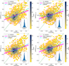 |
Fig. 16 Comparison of the Gaia-ESO [Ca/Fe] with the Gaia uncalibrated (top left), calibrated (top right), Teff-calibrated (bottom left) and log g-calibrated (bottom right) [α/Fe], Symbols and colours are as in the Fig. 11. |
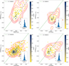 |
Fig. 17 Comparison of the Gaia-ESO [X/Fe] with the Gaia uncalibrated [X/Fe] for the following chemical species (from top to bottom, left to right): Mg, Si, Ca, and Ti. Symbols and colours are as in the Fig. 11. |
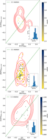 |
Fig. 18 Comparison of the Gaia-ESO [X/Fe] with the Gaia uncalibrated [X/Fe] for the following chemical species (from top to bottom): Cr, Ni, and Ce. Symbols and colours are as in the Fig. 11. |
6 Asteroseismic targets
Part of the legacy of GES has been the creation of new reference sets of stellar parameters. In particular, collaborations between asteroseismology and spectroscopy aim at providing atmospheric parameters using both spectroscopic and asteroseismic data, derived iteratively and converging on Teff, log g and [Fe/H] for stars targeted by GES selected from the K2 and CoRoT projects. This resulted in two reference sets: 90 stars from the K2 at Gaia-ESO project (Worley et al. 2020), and 1599 stars from the CoRoT at Gaia-ESO project (Masseron et al, in prep). These samples were observed in Gaia-ESO as either high resolution (hereafter, the K2 or CoRot ‘HR’ sample) with UVES or medium resolution (hereafter, the K2 or CoRoT ‘MR’ sample) with GIRAFFE.
The results obtained from the HR and MR reference samples reflect the different quality, e.g. the S/N, and the wavelength coverage of the spectra that was used to derive them. The MR spectra are typically obtained for fainter stars and they cover a small wavelength range, while HR spectra correspond to the brightest targets and cover a spectral range of about 2000 Å. Further discussion about the comparisons of the parameters between HR and MR for the K2 sample are given in Worley et al. (2020). Note that none of the MR K2 stars are present in Gaia DR3.
Figure 23 compares the log g for the K2 and CoRoT reference sets with the values obtained by Gaia-ESO and the two sets of values generated by GSP-Spec, log g uncalibrated and log g calibrated. We note that a very good agreement is obtained between the GES and seismic log g, on the one hand, and between the Gaia calibrated and seismic log g for the K2 HR sample with a mean difference less than 0.05 in absolute value. An offset of −0.27 exists between the GES and seismic log g for the K2 MR sample, while an offset of −0.25 is found between the Gaia uncalibrated and seismic log g for the K2 HR sample. An offset larger than 0.1 is found for the six comparisons with CoRot reference stars. For eight out of the ten comparisons shown in Fig. 23, the standard deviation of the difference is larger than 0.25.
Figure 24 shows the same kind of comparison but for the metallicity. Four estimates of [Fe/H] or [M/H] are compared to the seismic estimate, namely the GES metallicity, and the Gaia uncalibrated, calibrated and OC-calibrated ones. In all cases, the offsets are below 0.1 in absolute value, with a standard deviation of the difference between 0.05 and 0.15. We can therefore conclude in a good agreement between the spectroscopic estimates of the metallicity and those based on spectral analysis adopting seismic surface gravities.
In summary, the comparison of spectroscopic and seismic surface gravities reveals significant offsets, of different sign, for most tested estimates. At this stage, it is impossible to use the seismic data to argue in favour of one of the two GSP-Spec gravity scales. On the other hand, the comparison of spectroscopic and seismic metallicities let us think that all scales are more or less equivalent. This comparison shows that the multi-messenger approach to building reference sets of stellar parameters provides a useful validation of survey results, but yet there is no unanimous agreement between Gaia data and spectroscopic data combined with asteroseismology. Further development and expansion of these sets is required.
Statistical quantities for the quantities Δ𝒫 where 𝒫 is Teff, log g, [Fe/H], [Ca/Fe] computed for two G-magnitude ranges.
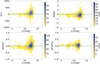 |
Fig. 19 Difference between Gaia and Gaia-ESO parameters Δ𝒫 = 𝒫Gaia − 𝒫GES as a function of the G magnitude (blue dots) where 𝒫 is, from left to right and top to bottom, Teff, log g, [Fe/H], [Ca/Fe]. The dashed black horizontal line has equation Δ𝒫 = 0. |
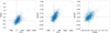 |
Fig. 20 Δ𝒫′ vs. Δ𝒫 where 𝒫 and 𝒫′ are chosen among Teff, log g, [Fe/H]. The dashed black horizontal and vertical line have equation Δ𝒫 = 0 and Δ𝒫′ = 0. Here we use the Gaia calibrated log g and the uncalibrated [M/H]. |
7 Stars in open star clusters: individual abundances and average properties
7.1 Open cluster member stars in common
As shown in Fig. 6, a large fraction of stars in common between the two surveys belong to open star clusters. Among them, we have selected those which are highly probable members of clusters in order to compare both the metallicity and the abundances of individual members, as well as the average properties of the open clusters. For GES, we used the membership analysis of Jackson et al. (2022) available for most clusters, and of Viscasillas Vázquez et al. (2022) for the remaining ones. In both cases, the membership probability was calculated considering, at the same time, the GES radial velocities and the Gaia proper motions and parallaxes. We cross-matched the member stars from GES with the Gaia database, finding that there are 136 member stars of open clusters which have GES and GSP-Spec stellar parameters. They belong to 34 different open clusters. In the following analysis, we only consider member stars observed by GES with the high-resolution setups, i.e. observed with an UVES setup.
In Fig. 25, we show the Gaia metallicities [M/H] (uncalibrated, calibrated, and OC-calibrated) as a function of GES [Fe/H]. As seen earlier for the selection 𝒮3, we find a good agreement between the GES metallicity scale and the three different Gaia metallicity scale. The mean difference is not null but negligible given the cumulated uncertainty of the metallicity estimates. For a lower number of stars, which varies from element to element, we also have some individual elemental abundances. They are shown in Fig. 26 for Mg, Si, Ca, Ti and Ni in which both abundances of individual member stars and averaged values per clusters are shown. The agreement between GES and Gaia abundances is in general difficult to judge given the low statistics per cluster. We note that in general keeping individual measurements with a GSP-Spec abundance quality flag set to 0 (best case) removes most of the discordant values; this is not true for Ti where this filtering is not enough to reduce the scatter. If one looks at the per-cluster averaged quantities (right column), then the agreement for Ca is good. This shows that the somewhat imprecise GSP-Spec abundances due to its medium-resolution spectroscopy, and the faint G regime of the current sample can be counterbalanced by working with averaged quantities. Stellar clusters are an example of science case where averaging abundances is suitable.
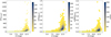 |
Fig. 21 Correlation between e(𝒫Gaia) and G where 𝒫 if either Teff, log g or [M/H] (from left to right). |
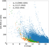 |
Fig. 22 GES S/N and RVS S/N as a function of G for respectively 112 990 (blue) and 1117 (orange) objects of 𝒮0 with a valid GES (resp., RVS) S/N and RVS S/N as a function of G for the 552 (green) objects of 𝒮3 with a valid RVS S/N. |
7.2 Average metallicity and [α/Fe] of clusters in common
In this section, we compare the abundance properties of open clusters in common between GES and Gaia. To compute the average metallicity and [α/Fe] of clusters observed by Gaia, we performed the membership analysis starting from the 2681 clusters (270487 stars) catalogued in Cantat-Gaudin et al. (2020). The membership probability was derived using the parallax and proper motion distributions, and then validated using skycoordinates. We obtained 7823 members (1334 OCs) which have Gaia GSP-Spec stellar parameters. We selected the stars belonging to the high- and medium-quality samples defined as a combination of Gaia flags in Gaia Collaboration (2023b) and also adopted in Viscasillas Vázquez et al. (2023), which reduces the sample to 3718 stars (998 OCs). For this test, we select only clusters older than 0.1 Gy to avoid problems related to the uncertain cluster membership and to the spectral analysis of young stars (e.g., activity hampering the determination of photospheric abundances). Among the 998 OCs, there are 52 clusters in common with the 62 clusters of Gaia-ESO with age ≥ 0.1 Gy (see, e.g. Magrini et al. 2023). Figure 27 shows the average metallicities of the sample of 52 clusters, computed using for each open cluster the metallicity of all available member stars in the GES catalogue or in the Gaia catalogue. In other words, now, we compare the GES and Gaia average metallicity of given open cluster, computed with a different selection of member stars. In particular, for the 52 clusters, we found 624 members in Gaia and 679 in Gaia-ESO. We note that the agreement between the GES metallicity scale and the three GSP-Spec metallicity scales is rather good, and slightly better (smaller bias) when considering the calibrated metallicities. We also examined whether the number of members used to calculate the average metallicity could influence the scatter of the distributions. Clusters with fewer than three members (18 out of 52) are displayed in the background in light gray and are indeed the reason for the scatter around the 1-to-1 line. Among clusters with at least three member stars, there are only three clusters with |Δ[Fe/H]| > 0.2: NGC 6281 and NGC 2516, whose abundance are underestimated by Gaia compared to Gaia-ESO and NGC 2243, whose abundance is instead overestimated. The above findings are compatible with our remarks in the previous subsections: the computation of GSP-Spec average abundances gives values well correlated with averages obtained with a higher-resolution survey like Gaia-ESO. In the three clusters with the most significant differences in metallicity, we note: NGC 2516 has 25 stars in Gaia and 16 in GES, in which all of the latter are MS stars, as expected for a young cluster; while the former sample contains sources with temperatures from about 4000 to 8000 K, and gravities between 0.6 and 5. Thus, some of them must be contaminants. Furthermore, since NGC 2516 is young and close, we do not expect such low abundances as those measured by Gaia. For NGC 6821, we have data on three stars from GES and eight stars from Gaia. The stars observed by Gaia have Teff reaching up to about 8000 K, a range in which metallicities are often underestimated, which may explain why Gaia abundances are lower. Finally, for NGC 2243 we compare 19 stars in GES (both MS and giants) vs. three in Gaia, which are all giants. The abundances in GES are in better agreement with literature values (François et al. 2013).
Figure 28 shows the comparison [α/Fe] for the 52 open clusters. The values are located in the range [−0.2, 0.2]. Given the uncertainties on each mean [α/Fe], we note a good agreement between the GES abundance scale and the two Gaia ones (uncalibrated and calibrated). Nevertheless, the offset is closer to zero when the GES quantities are compared to the Gaia calibrated ones rather than to the uncalibrated. We identify four clusters in strong disagreement: Tombaugh 2, Blanco 1, NGC 6067 and NGC 6404. To estimate the quality of the Gaia data, we used the HQ (High Quality) and MQ (Medium Quality) indicators, which are derived from a combination of Gaia GSP-Spec flags and defined in Gaia Collaboration (2023b, see their Appendix B for a complete definition of the ranges of the used GSP-Spec flags to produce the HQ and MQ samples). The MQ sample defined in Gaia Collaboration (2023b) contains about ~41000000 stars with median uncertainty in [M/H] of about 0.06 dex and median uncertainty in [α/Fe] of about 0.04 dex, while the HQ sample stars (~2 200 000) have with very low parameter uncertainties, in particular a median uncertainty in [M/H] ~ 0.03 dex and ~0.015 dex in [α/Fe].
For Tombaugh 2, only two member stars with MQ or HQ=1 have an uncalibrated [α/Fe] and only one member star has a calibrated [α/Fe], while nine member stars have a GES [α/Fe]. These low statistics is likely the reason of the disagreement. We remind that Tombaugh 2 is one of the most distant known clusters (see, e.g. Frinchaboy et al. 2008). In Blanco 1, there are six member stars with Gaia parameters (HQ and/or MQ=1). The average [α/Fe] are very similar for the uncalibrated and the calibrated cases, (0.26 ± 0.14) dex and (0.24 ± 0.17) dex, respectively, and (0.25 ± 0.13) dex for [Ca/Fe]. GES observed 16 member stars in Blanco 1, with an average [α/Fe] = (0.015 ± 0.069) dex. Therefore, the difference is larger than 3σ. NGC 6067 has eight member stars with Gaia (HQ and/or MQ=1) α abundance, to be compared to 13 members in GES. The average values of [α/Fe] are −0.14 dex and −0.19 dex for Gaia uncalibrated and calibrated, respectively, and 0.08 dex for GES. The agreement of Gaia [α/Fe] with GES [Ca/Fe] = −0.08 dex is better. NGC 6404 has three member stars with a Gaia (HQ and/or MQ=1) α abundance and four member stars in GES. The average values of [α/Fe] are −0.12 dex (uncalibrated) and −0.10 dex (calibrated) for Gaia versus 0.18 dex for GES; the disagreement is not solved (but less drastic) if we compare these GSP-Spec abundances to GES Ca since GES gives [Ca/Fe] = 0. In addition, for three of the four clusters considered (excluding Blanco 1), the observed stars are low-gravity giants. This could lead to a bias introduced by the standard spectroscopic analysis in which usually 1D atmospheric models in Local Thermodynamical equilibrium (LTE) approximation are adopted. These approximations are often not adequate to analyse giant and/or low metallicity stars (see, e.g. Casali et al. 2020; Magrini et al. 2023). The only exception where the discrepancy is not easy to justify is the case of Blanco 1, since both in GES and Gaia stars with log g around 4 are observed. However, Blanco 1 is a very young cluster, with an age ~0.1 Gy, i.e. the lower bound age of our selection. Very young stars are known to present difficulties in their analysis Baratella et al. (2020, 2021); Spina et al. (2020), which may explain the differences in results. As in Figure 27, clusters with less than three members in both samples (21 out of 52) are in light grey. Their exclusion reduces, as for metallicity, the scatter around the 1-to-1 line.
Considering that Ca is the largest contributor to the Gaia [α/Fe] estimate, we now compare the average Gaia [α/Fe] to the average GES [Ca/Fe] in Fig. 29. The overall agreement is also satisfactory. However, Tombaugh 2 and Blanco 1 remain α-enhanced in Gaia compared to GES. The same argument (low gravity stars) as in the previous paragraph can be proposed as the source of the abundance discrepancy.
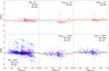 |
Fig. 23 Comparison of log g values as a difference to the reference seismic values (K2 or CoRoT) for each of Gaia-ESO, Gaia uncalibrated and Gaia calibrated. Top row: comparison with K2; bottom row: comparison with CoRoT. The HR (red) and MR (blue) reference samples are shown. |
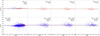 |
Fig. 24 Comparison of [Fe/H] values as a difference to the reference seismic values (K2 or CoRoT) for Gaia-ESO, Gaia, Gaia calibrated, and Gaia OC-calibrated. Top row: comparison with K2; bottom row: comparison with CoRoT. The HR (red) and MR (blue) reference samples are shown. |
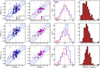 |
Fig. 25 GES vs. Gaia metallicity (uncalibrated, calibrated, and calibrated with open clusters) for 136 stars belonging to 34 open clusters in common. The panels on the left show the member stars individually and the average metallicities per cluster, and the panels on the right show the histograms of the metallicity distributions of both samples and their difference Δ. The size of the symbols is proportional to the number of members. The light-blue bands indicate an agreement between ± 0.2. |
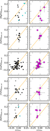 |
Fig. 26 Calibrated abundance ratios [X/Fe] from Gaia versus those from Gaia-ESO for individual members of open clusters in common (left) and their average abundance ratios (right). Each symbol represents a single member star coloured according to its quality flag (black: 0, grey: 1, cyan:2). |
8 The properties of the open cluster population from the combined Gaia-GES datasets
The purpose of this section is to illustrate the scientific potential of Gaia, and the possibility of combining Gaia RVS results with those of ground-based spectroscopic surveys, with appropriate choices in stellar parameters and abundances. Given the agreement between the GES and Gaia abundance ratios, in this section we check what kind of general properties of the open cluster population can be retrieved from the Gaia abundances, such as the radial metallicity and [α/Fe] gradients, the trend of [α/Fe] as a function of metallicity, and the age-metallicity relation. In our analysis, we use [Ca/Fe] as a proxy for [α/Fe] for both Gaia and GES. We limit our sample to clusters with ages between 1 and 3 Gy to avoid the problems related to the analysis of the youngest stars and the issue of migration for the oldest clusters as discussed in Magrini et al. (2023). For the open clusters observed with Gaia we consider only clusters with at least three member stars.
Open clusters can, indeed, be considered among the best tracers of the chemical properties of the thin-disc stellar populations of our Galaxy, including the spatial distribution of elemental abundances. Since about five decades ago, many works have exploited the use of open clusters to trace radial metallicity and abundance gradients (see e.g. Mayor 1976; Janes 1979; Janes et al. 1988; Friel & Janes 1993; Carraro & Chiosi 1994; Friel 1995; Twarog et al. 1997; Friel et al. 2002; Donor et al. 2020; Spina et al. 2021; Magrini et al. 2023; Joshi et al. 2024, among many works). The strength of open clusters – precise ages and distances – is, indeed, maximised by spectroscopic observations at medium and high spectral resolution. For this reason, many clusters have been observed by large spectroscopic surveys, such as APOGEE, GALAH and GES. An even larger number of open clusters will be spectroscopically observed in the forthcoming years thanks to instruments dedicated to spectroscopic surveys, such as WEAVE (Dalton et al. 2018) and 4MOST (de Jong et al. 2019). A recent review of the state of the art of the radial metallicity gradient obtained with open clusters from the three main current high-resolution spectroscopic surveys (GES, APOGEE, and GALAH) has been presented in Spina et al. (2022).
In Figure 30, we compare the overall trends of the open cluster population observed by Gaia and by GES. The open clusters observed by Gaia are located between ~ 6 and 12.5 kpc, while those observed by Gaia-ESO reach further distances. The two samples continuously follow the same decreasing radial metallicity gradient, and the same increasing trend of [Ca/Fe] with RGC. The shape of the metallicity gradient in Fig. 30 shows a bimodal distribution, with a knee – the radius at which there is a change of slope in the gradient from steep to almost flat – located at around 11–12 kpc. The shape of the gradient represents an important observational constraint for defining the timescales of the formation of the Galactic thin disc, the radial variations and efficiency of the star formation rate and of the balance between gas inflow and outflow. Several works confirmed the presence of the gradient break located between 10 to 12 kpc (e.g. Bragaglia et al. 2008; Sestito et al. 2008; Friel et al. 2010; Pancino et al. 2010; Carrera & Pancino 2011; Yong et al. 2012; Frinchaboy et al. 2013; Reddy et al. 2016; Magrini et al. 2017, 2023; Casamiquela et al. 2019; Donor et al. 2020; Zhang et al. 2021b; Netopil et al. 2022; Spina et al. 2022; Myers et al. 2022; Carbajo-Hijarrubia et al. 2024). We computed a weighted linear fit to our combined dataset, with a two-slope function. We obtained a slope −0.060 ± 0.013 dex kpc−1 in the inner region and −0.027 ± 0.011 dex kpc−1 in the outer region, with the separation at about 12 ± 1.5 kpc (computed as in Magrini et al. 2023 with the ELBOW method5). The position of the knee identified by our sample is in excellent agreement with that of Spina et al. (2022), Rknee = 12.1 ± 1.1 kpc, as well as the inner slope −0.064 ± 0.007 dex kpc−1 and the outer slope −0.019 ± 0.008 dex kpc−1.
In the lower panel, a growth of [Ca/Fe] can clearly be seen from the inner part to the outer part of the Milky Way, with an increment of about 0.25 dex in [Ca/Fe]. This behaviour is also observed in the APOGEE sample (RGC range 7–12 kpc, Donor et al. 2018), in the OCCASO sample (6–11 kpc, Casamiquela et al. 2019) and in the GES sample of (5–20 kpc, Magrini et al. 2023) for different α elements. The slopes are 0.019±0.005 dex kpc−1 in the inner part and 0.012±0.009 dex kpc−1 in the outer one. This, together with the metallicity gradient, is a clear indication of inside-out disc formation (Chiappini et al. 1997; Minchev et al. 2013, 2014), in which inner regions were enriched more rapidly in both iron and α elements, while the outer one had a lower star formation efficiency with a delayed production of elements with longer production time scales, such as iron (see also, Tinsley 1979; Greggio & Renzini 1983; Matteucci & Greggio 1986).
The age-metallicity relation (AMR) in the Galactic disc is crucial to understand how the chemical evolution of the Galaxy proceeded in time. Star clusters provide a useful tool for studying the AMR as they offer a chronological sequence. Previous studies, spanning the last two decades, have explored this relationship using open clusters. While some earlier research found no distinct AMR (Friel et al. 2010; Yong et al. 2012), others suggested a weak correlation (Zhong et al. 2020). Joshi et al. (2024) combined a large sample of open cluster parameters, including ages and metallicities, and inferred their AMR. Although there is great scatter in their relationship, they found that for clusters older than 0.25 Gy, there is a decreasing trend in metallicity with increasing cluster age. In Figure 31, we show the age-metallicity relation (AMR) for the sample of open clusters with ages in the range [1 Gy, 3 Gy]. Considering the clusters all together, we also find a considerable scatter in metallicity at each age. If we divide the clusters into galactocentric distance bins, however, we find much better-defined AMRs. In Figure 31, our clusters are divided in three radial bins: the inner bin with RGC < 7 kpc, the central one with 7 kpc ≤ RGC ≤ 9 kpc, and the outer one with RGC ≥ 9 kpc. We note a loose correlation: the youngest clusters tend to have a [M/H] higher than the oldest ones. Both the GES and the Gaia cluster populations support this correlation. Compared to Joshi et al. (2024), we are considering the end of the tail of the open cluster age distribution, having only clusters between 1–3 Gy. We confirm their result, but thanks to the radial bin separation, we can explain the origin of the scatter in the AMR.
In Figure 32 we show the Gaia and GES clusters in the [Ca/Fe] vs. [M/H] and in the [α/Fe] vs. [M/H] planes. In the background, we show the abundances of the field stars observed by Gaia-ESO, selected according to these conditions: GES_FLD is MW, setup is U580, S/N > 20, error on [Fe/H] < 0.2, and errors on the individual abundances < 0.1 (about 3000 stars). We classified the field stars according to their belonging to the thin, thick and high-α discs using a set of supervised learning techniques such as the support vector machines (SVMs) (Boser et al. 1992), already adopted in Viscasillas Vázquez et al. (2022). We defined a training set based on the sample of Costa Silva et al. (2020), with [α/Fe]-[Fe/H] derived by Delgado Mena et al. (2017). We included the thin and thick disc populations, as well a high-α metal-rich population (hαmr). We obtained an accuracy in the classification of 100%. We trained the SVM in the multiclass case with a RADIAL BASIS FUNCTION (RBF) and implemented using the SCIKIT-LEARN package (Pedregosa et al. 2011). We calculated the membership probabilities (see Tables A.2 and A.3) calibrated using Platt scaling extended for multi-class classification (Wu et al. 2004); we then transfer the classification probability to the open cluster population. This allows us to place the open clusters of GES and most of the Gaia ones in the thin-disc or hαmr populations. The classification is obtained in the [α/Fe]-[Fe/H] plane in which the separation among the populations is more clear, but it can be transferred also to the [Ca/Fe]-[Fe/H] plane. We find that the selected open-cluster population belongs to the thin disc, as expected from their orbital properties (e.g. Wu et al. 2009).
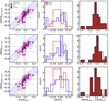 |
Fig. 27 GES vs. Gaia metallicity (uncalibrated in the upper panel, calibrated in the central panel and OC-calibrated in the bottom panel) for 52 open clusters in common: 34 clusters with 3 or more members for both spectroscopic surveys are shown in magenta, while the 18 clusters with less than 3 members in one of the two surveys are in light grey. Left: Gaia vs. GES average cluster metallicities; centre: metallicity distributions of the clusters as seen in GES (red) and in Gaia (blue); right: distribution of the averaged-metallicity differences Δ[Fe/H] = [Fe/H]Gaia − [Fe/H]GES. |
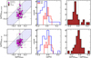 |
Fig. 28 GES vs. Gaia [α/Fe] (uncalibrated, calibrated) for 52 open clusters in common. Left: average [α/Fe] per cluster; centre: histograms of the [α/Fe] distributions of both samples; right: histograms of the difference Δ[α/Fe]. |
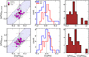 |
Fig. 29 GES [Ca/Fe] vs. Gaia [α/Fe] (uncalibrated, calibrated) for 52 open clusters in common. Similar panels as in Fig. 28. |
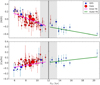 |
Fig. 30 Metallicity and [Ca/Fe] as a function of the Galactocentric radius for the sample of Gaia and GES open clusters with 1 Gy < age < 3 Gy. In the upper panel, we show [M/H] (calibrated metallicity for Gaia and [Fe/H] for GES) as a function of RGC, while in the bottom panel, we present [Ca/Fe] versus RGC. The weighted linear fits are shown with continuous lines. The vertical line mark the location of the ELBOW. The size of the symbols is proportional of the number of member stars used to compute the mean values. |
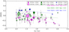 |
Fig. 31 Age-Metallicity relation for the sample of clusters with ages between 1 and 3 Gy, divided in three radial bins. The clusters observed by Gaia are represented with semi-transparent circles, while those observed by GES with solid-filled circles. The linear regressions are shown with dashed lines using the same colour as the corresponding radial bin. In the plot, we show the coefficients of the three age-metallicity relationships. The size of the symbols is proportional of the number of member stars used to compute the mean values. |
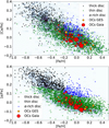 |
Fig. 32 Gaia and GES clusters in the [Ca/Fe] vs. [M/H] (upper panel) and in the [α/Fe] vs. [M/H] (lower panel) planes. In the background (light blue 2D histogram with rectangular cells), we show the abundances of the field stars observed by GES. In black, we show the thick disc population; in green, the thin disc one; in blue, the high-α discs. The open clusters observed by GES are represented by orange circles and those observed by Gaia by red circles. In both cases the radius of the circles is proportional to the number of members. |
9 Conclusions
This article focuses on assessing the quality and on a scientific usage of the observables measured or inferred from the Gaia mean spectra recorded with the Radial Velocity Spectrometer of resolving power R ~ 11 500. The quality assessment is carried out by comparing a number of Gaia DR3 spectroscopically derived quantities to their counterparts obtained with the ground-based higher-resolution spectroscopic survey Gaia-ESO. Thus, this study is primarily a new external and independent validation of the Gaia results. Here are the main results:
given the respective uncertainties of the two surveys, we find an excellent agreement between the Gaia RVS radial velocities and the GES ones. We are not able to explain the discrepancy for only a very small number of objects, about 600 out of 14 692. This could be due to underestimated uncertainties in one or both surveys, or it can hide a physical origin (jitter, hidden multiplicity);
Gaia DR3 still misses most of the spectroscopic binaries (SB) present in the GES – Gaia intersection: only 22 out of the 2117 GES SBn (preliminary results for the final GES SB census) are flagged as (astrometric or eclipsing or spectroscopic) binaries by Gaia. We find an empirical efficiency of the DSC classifier compatible with the theoretical efficiency: about 0.2% of the unresolved binaries are recovered by this classifier. The RUWE quantity is not a sufficient criterion to spot potential SBn;
the broadening parameter is loosely correlated with the projected rotational velocity of the stars since the sample under analysis has a bias towards FGK stars that generally have low rotational velocities, and thus we are reaching the instrumental limit in spectral resolution to measure rotational velocities;
our comparison sample shows a better agreement between the GES and GSP-Spec sets of parameters (effective temperature, surface gravity, metallicity) for objects brighter than G = 11 mag than for objects fainter than G = 11 mag. It tends to indicate that for objects fainter than G = 11 mag, the accuracy and/or the precision of the atmospheric parameters of Gaia GSP-Spec degrade quickly. This magnitude threshold corresponds to a S/N of the mean RVS spectra of about 70 ± 20. The final users should be cautious when they want to work with these parameters for faint objects. The use of the GSP-Spec calibrations and flag systems is mandatory to avoid interpretation mistakes;
using asteroseismic-based quantities did not allow us to reconcile unequivocally the different log g and [Fe/H] scales under study. The best agreement is obtained between the calibrated gravity of Gaia and those from the HR sample of GES, with an offset close to zero for the K2 sample and slightly positive for the CoRoT one. For metallicity, offsets are equally small (but with sign change) in the comparison with all Gaia calibrations, both for K2 and CoRoT samples. The scatter tends to increase for the GES MR sample. An effort of the community is still needed to increase the collection of reference stars for which independent techniques are used to estimate their atmospheric parameters that can be used afterwards for cross-survey calibrations;
based on our limited sample, the improvement brought by the calibrated GSP-Spec parameters is important for the surface gravity, while it is not so evident for the abundances;
the situation is better for abundance ratios. Indeed, it is empirically known that systematic effects tend to cancel out for abundance ratios. It is therefore probably safer to work with faint objects if one focuses on these quantities. Here again, the GSP-Spec flags should be used to further clean the selection;
in particular, using averaged abundances for open clusters allow us to retrieve well-known properties of this stellar population, providing a scientific check of the Gaia GSP-Spec data quality and showing that this spectroscopic survey can be combined to other ground-based spectroscopic surveys to explore the properties of Milky Way stellar populations.
Acknowledgements
Institutional: The authors thank the referee for their very careful reading and their detailed commentary. It was really of great help to improve this article. CVV and LS thank the EU programme Erasmus+ Staff Mobility for their support. CVV and GT acknowledge funding from the Research Council of Lithuania (LMTLT, grant No. P-MIP-23-24). We acknowledge financial support under the National Recovery and Resilience Plan (NRRP), Mission 4, Component 2, Investment 1.1, Call for tender No. 104 published on 2.2.2022 by the Italian Ministry of University and Research (MUR), funded by the European Union – NextGenerationEU – Project ‘Cosmic POT’ Grant Assignment Decree No. 2022X4TM3H by the Italian Ministry of Ministry of University and Research (MUR). We acknowledge support from the INAF Large Grant 2023 “EPOCH” (PI: Magrini), from the INAF Mini Grant 2022 ‘Checs’ (PI Magrini), from the INAF funds to support WEAVE preparation. Consortium: Based on dataproducts from observations made with ESO Telescopes at the La Silla Paranal Observatory under programmes 188.B-3002, 193.B-0936, and 197.B-1074. These data products have been processed by the Cambridge Astronomy Survey Unit (CASU) at the Institute of Astronomy, University of Cambridge, and by the FLAMES/UVES reduction team at INAF/Osservatorio Astrofisico di Arcetri. These data have been obtained from the Gaia-ESO Survey Data Archive, prepared and hosted by the Wide Field Astronomy Unit, Institute for Astronomy, University of Edinburgh, which is funded by the UK Science and Technology Facilities Council. This work was partly supported by the European Union FP7 programme through ERC grant number 320 360 and by the Leverhulme Trust through grant RPG-2012-541. We acknowledge the support from INAF and Ministero dell’Istruzione, dell’Università e della Ricerca (MIUR) in the form of the grant “Premiale VLT 2012”. This work has made use of data from the European Space Agency (ESA) mission Gaia (https://www.cosmos.esa.int/gaia), processed by the Gaia Data Processing and Analysis Consortium (DPAC, https://www.cosmos.esa.int/web/gaia/dpac/consortium). Funding for the DPAC has been provided by national institutions, in particular the institutions participating in the Gaia Multilateral Agreement. Databases: This research has made use of NASA’s Astrophysics Data System Bibliographic Services. This research has made a heavy use of the SIMBAD database, the VizieR catalogue access tool and the cross-match service provided and operated at CDS, Strasbourg, France. Softwares: This work has made use of python 3.x (https://www.python.org) (Van Rossum & Drake 2009) and of the following python s modules: Astropy (https://www.astropy.org), a community-developed core Python package and an ecosystem of tools and resources for astronomy (Astropy Collaboration 2013, 2018, 2022); matplotlib (https://matplotlib.org/) (Hunter 2007); numpy (https://numpy.org/) (Harris et al. 2020); scipy (https://scipy.org/) (Virtanen et al. 2020); Scikit-learn Machine Learning (Pedregosa et al. 2011); StatsModels (Seabold & Perktold 2010); Seaborn (Waskom 2021). This work has made use of TopCat (Taylor 2005).
Appendix A Additional material
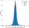 |
Fig. A.1 Probability distribution of the normalised velocity differences. The blue histogram (bin width = 0.1) displays the distribution Δnormυrad of the difference of the radial velocity differences υrad,Gaia − υrad,GES normalised by the propagated errors |
![$\[\sqrt{\sigma\left[v_{\mathrm{rad}, \mathrm{Gaia}}\right]^2+\sigma_{\mathrm{corr}}\left[v_{\mathrm{rad}, \mathrm{GES}}\right]^2}\]$](/articles/aa/full_html/2024/10/aa50357-24/aa50357-24-eq9.png)
Main columns of the Gaia-ESO and Gaia public catalogues used in this study.
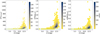 |
Fig. A.2 Correlation between e(𝒫Gaia) and GRVS where 𝒫 if either Teff, log g or [M/H] (from left to right). |
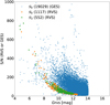 |
Fig. A.3 GES S/N and RVS S/N as a function of G for respectively 19 029 (blue) and 1117 (orange) objects of 𝒮0 with a valid GES (resp., RVS) S/N and RVS S/N as a function of G for the 552 (green) objects of 𝒮3 with a valid RVS S/N. |
SVM classification of the GES open clusters (aged between 1 and 3 Gy) according to the given training data and predicted probabilities of belonging to each of of the disk components (thin: P0, thick: P1, and hα: P2)
SVM classification of 67 Gaia open clusters (aged between 1 and 3 Gy and with N≥3) according to the given training data and predicted probabilities of belonging to each of the disk components (thin: P0, thick: P1, and hα: P2)
References
- Abdurro’uf, Accetta, K., Aerts, C., et al. 2022, ApJS, 259, 35 [NASA ADS] [CrossRef] [Google Scholar]
- Ahn, C. P., Alexandroff, R., Allende Prieto, C., et al. 2014, ApJS, 211, 17 [NASA ADS] [CrossRef] [Google Scholar]
- Andrae, R., Fouesneau, M., Creevey, O., et al. 2018, A&A, 616, A8 [NASA ADS] [CrossRef] [EDP Sciences] [Google Scholar]
- Andrae, R., Fouesneau, M., Sordo, R., et al. 2023, A&A, 674, A27 [CrossRef] [EDP Sciences] [Google Scholar]
- Anguiano, B., Majewski, S. R., Allende Prieto, C., et al. 2018, A&A, 620, A76 [NASA ADS] [CrossRef] [EDP Sciences] [Google Scholar]
- Astropy Collaboration (Robitaille, T. P., et al.) 2013, A&A, 558, A33 [NASA ADS] [CrossRef] [EDP Sciences] [Google Scholar]
- Astropy Collaboration (Price-Whelan, A. M., et al.) 2018, AJ, 156, 123 [Google Scholar]
- Astropy Collaboration (Price-Whelan, A. M., et al.) 2022, ApJ, 935, 167 [NASA ADS] [CrossRef] [Google Scholar]
- Babusiaux, C., Fabricius, C., Khanna, S., et al. 2023, A&A, 674, A32 [NASA ADS] [CrossRef] [EDP Sciences] [Google Scholar]
- Bailer-Jones, C. A. L., Rybizki, J., Fouesneau, M., Demleitner, M., & Andrae, R. 2021, AJ, 161, 147 [Google Scholar]
- Baratella, M., D’Orazi, V., Carraro, G., et al. 2020, A&A, 634, A34 [NASA ADS] [CrossRef] [EDP Sciences] [Google Scholar]
- Baratella, M., D’Orazi, V., Sheminova, V., et al. 2021, A&A, 653, A67 [NASA ADS] [CrossRef] [EDP Sciences] [Google Scholar]
- Bashi, D., Shahaf, S., Mazeh, T., et al. 2022, MNRAS, 517, 3888 [NASA ADS] [CrossRef] [Google Scholar]
- Blomme, R., Daflon, S., Gebran, M., et al. 2022, A&A, 661, A120 [NASA ADS] [CrossRef] [EDP Sciences] [Google Scholar]
- Bonifacio, P., Caffau, E., Spite, M., et al. 2018, A&A, 612, A65 [NASA ADS] [CrossRef] [EDP Sciences] [Google Scholar]
- Boser, B. E., Guyon, I. M., & Vapnik, V. N. 1992, in Proceedings of the Fifth Annual Workshop on Computational Learning Theory, COLT ’92 (New York, NY, USA: Association for Computing Machinery), 144 [CrossRef] [Google Scholar]
- Bragaglia, A., Sestito, P., Villanova, S., et al. 2008, A&A, 480, 79 [NASA ADS] [CrossRef] [EDP Sciences] [Google Scholar]
- Bressan, A., Marigo, P., Girardi, L., et al. 2012, MNRAS, 427, 127 [NASA ADS] [CrossRef] [Google Scholar]
- Buder, S., Sharma, S., Kos, J., et al. 2021, MNRAS, 506, 150 [NASA ADS] [CrossRef] [Google Scholar]
- Cantat-Gaudin, T., Anders, F., Castro-Ginard, A., et al. 2020, A&A, 640, A1 [NASA ADS] [CrossRef] [EDP Sciences] [Google Scholar]
- Carbajo-Hijarrubia, J., Casamiquela, L., Carrera, R., et al. 2024, A&A, 687, A239 [NASA ADS] [CrossRef] [EDP Sciences] [Google Scholar]
- Carraro, G., & Chiosi, C. 1994, A&A, 287, 761 [NASA ADS] [Google Scholar]
- Carrera, R., & Pancino, E. 2011, A&A, 535, A30 [NASA ADS] [CrossRef] [EDP Sciences] [Google Scholar]
- Casali, G., Magrini, L., Frasca, A., et al. 2020, A&A, 643, A12 [NASA ADS] [CrossRef] [EDP Sciences] [Google Scholar]
- Casamiquela, L., Blanco-Cuaresma, S., Carrera, R., et al. 2019, MNRAS, 490, 1821 [NASA ADS] [CrossRef] [Google Scholar]
- Chiappini, C., Matteucci, F., & Gratton, R. 1997, ApJ, 477, 765 [Google Scholar]
- Cirasuolo, M., Fairley, A., Rees, P., et al. 2020, The Messenger, 180, 10 [NASA ADS] [Google Scholar]
- Contursi, G., de Laverny, P., Recio-Blanco, A., & Palicio, P. A. 2021, A&A, 654, A130 [NASA ADS] [CrossRef] [EDP Sciences] [Google Scholar]
- Costa Silva, A. R., Delgado Mena, E., & Tsantaki, M. 2020, A&A, 634, A136 [EDP Sciences] [Google Scholar]
- Creevey, O. L., Sordo, R., Pailler, F., et al. 2023, A&A, 674, A26 [NASA ADS] [CrossRef] [EDP Sciences] [Google Scholar]
- Cropper, M., Katz, D., Sartoretti, P., et al. 2018, A&A, 616, A5 [NASA ADS] [CrossRef] [EDP Sciences] [Google Scholar]
- Cui, X.-Q., Zhao, Y.-H., Chu, Y.-Q., et al. 2012, Res. Astron. Astrophys., 12, 1197 [Google Scholar]
- Dalton, G. 2016, in Astronomical Society of the Pacific Conference Series, 507, Multi-Object Spectroscopy in the Next Decade: Big Questions, Large Surveys, and Wide Fields, eds. I. Skillen, M. Balcells, & S. Trager, 97 [Google Scholar]
- Dalton, G., Trager, S., Abrams, D. C., et al. 2018, in Ground-based and Airborne Instrumentation for Astronomy VII, 10702, eds. C. J. Evans, L. Simard, & H. Takami, International Society for Optics and Photonics (SPIE), 388 [Google Scholar]
- De Angeli, F., Weiler, M., Montegriffo, P., et al. 2023, A&A, 674, A2 [NASA ADS] [CrossRef] [EDP Sciences] [Google Scholar]
- de Jong, R. S., Agertz, O., Berbel, A. A., et al. 2019, The Messenger, 175, 3 [NASA ADS] [Google Scholar]
- De Silva, G. M., Freeman, K. C., Bland-Hawthorn, J., et al. 2015, MNRAS, 449, 2604 [NASA ADS] [CrossRef] [Google Scholar]
- Delchambre, L., Bailer-Jones, C. A. L., Bellas-Velidis, I., et al. 2023, A&A, 674, A31 [NASA ADS] [CrossRef] [EDP Sciences] [Google Scholar]
- Delgado Mena, E., Tsantaki, M., Adibekyan, V. Z., et al. 2017, A&A, 606, A94 [NASA ADS] [CrossRef] [EDP Sciences] [Google Scholar]
- Donor, J., Frinchaboy, P. M., Cunha, K., et al. 2018, AJ, 156, 142 [NASA ADS] [CrossRef] [Google Scholar]
- Donor, J., Frinchaboy, P. M., Cunha, K., et al. 2020, AJ, 159, 199 [NASA ADS] [CrossRef] [Google Scholar]
- Eyer, L., Audard, M., Holl, B., et al. 2023, A&A, 674, A13 [NASA ADS] [CrossRef] [EDP Sciences] [Google Scholar]
- Fouesneau, M., Frémat, Y., Andrae, R., et al. 2023, A&A, 674, A28 [NASA ADS] [CrossRef] [EDP Sciences] [Google Scholar]
- François, P., Pasquini, L., Biazzo, K., Bonifacio, P., & Palsa, R. 2013, A&A, 552, A136 [Google Scholar]
- Franciosini, E., Randich, S., de Laverny, P., et al. 2022, A&A, 668, A49 [NASA ADS] [CrossRef] [EDP Sciences] [Google Scholar]
- Frasca, A., Biazzo, K., Lanzafame, A. C., et al. 2015, A&A, 575, A4 [NASA ADS] [CrossRef] [EDP Sciences] [Google Scholar]
- Frémat, Y., Royer, F., Marchal, O., et al. 2023, A&A, 674, A8 [NASA ADS] [CrossRef] [EDP Sciences] [Google Scholar]
- Friel, E. D. 1995, ARA&A, 33, 381 [Google Scholar]
- Friel, E. D., & Janes, K. A. 1993, A&A, 267, 75 [NASA ADS] [Google Scholar]
- Friel, E. D., Janes, K. A., Tavarez, M., et al. 2002, AJ, 124, 2693 [NASA ADS] [CrossRef] [Google Scholar]
- Friel, E. D., Jacobson, H. R., & Pilachowski, C. A. 2010, AJ, 139, 1942 [NASA ADS] [CrossRef] [Google Scholar]
- Frinchaboy, P. M., Marino, A. F., Villanova, S., et al. 2008, MNRAS, 391, 39 [NASA ADS] [CrossRef] [Google Scholar]
- Frinchaboy, P. M., Thompson, B., Jackson, K. M., et al. 2013, ApJ, 777, L1 [NASA ADS] [CrossRef] [Google Scholar]
- Gaia Collaboration (Prusti, T., et al.) 2016, A&A, 595, A1 [NASA ADS] [CrossRef] [EDP Sciences] [Google Scholar]
- Gaia Collaboration (Arenou, F., et al.) 2023a, A&A, 674, A34 [CrossRef] [EDP Sciences] [Google Scholar]
- Gaia Collaboration (Recio-Blanco, A., et al.) 2023b, A&A, 674, A38 [CrossRef] [EDP Sciences] [Google Scholar]
- Gaia Collaboration (Vallenari, A., et al.) 2023c, A&A, 674, A1 [NASA ADS] [CrossRef] [EDP Sciences] [Google Scholar]
- Gilmore, G., Randich, S., Worley, C. C., et al. 2022, A&A, 666, A120 [NASA ADS] [CrossRef] [EDP Sciences] [Google Scholar]
- Greggio, L., & Renzini, A. 1983, Mem. Soc. Astron. Italiana, 54, 311 [NASA ADS] [Google Scholar]
- Harris, C. R., Millman, K. J., van der Walt, S. J., et al. 2020, Nature, 585, 357 [NASA ADS] [CrossRef] [Google Scholar]
- Hegedűs, V., Mészáros, S., Jofré, P., et al. 2023, A&A, 670, A107 [NASA ADS] [CrossRef] [EDP Sciences] [Google Scholar]
- Heiter, U., Jofré, P., Gustafsson, B., et al. 2015, A&A, 582, A49 [NASA ADS] [CrossRef] [EDP Sciences] [Google Scholar]
- Ho, A. Y. Q., Ness, M. K., Hogg, D. W., et al. 2017, ApJ, 836, 5 [NASA ADS] [CrossRef] [Google Scholar]
- Hourihane, A., François, P., Worley, C. C., et al. 2023, A&A, 676, A129 [NASA ADS] [CrossRef] [EDP Sciences] [Google Scholar]
- Hunter, J. D. 2007, Comput. Sci. Eng., 9, 90 [NASA ADS] [CrossRef] [Google Scholar]
- Jackson, R. J., Jeffries, R. D., Lewis, J., et al. 2015, A&A, 580, A75 [NASA ADS] [CrossRef] [EDP Sciences] [Google Scholar]
- Jackson, R. J., Jeffries, R. D., Wright, N. J., et al. 2022, MNRAS, 509, 1664 [Google Scholar]
- Janes, K. A. 1979, ApJS, 39, 135 [NASA ADS] [CrossRef] [Google Scholar]
- Janes, K. A., Tilley, C., & Lynga, G. 1988, AJ, 95, 771 [NASA ADS] [CrossRef] [Google Scholar]
- Jönsson, H., Holtzman, J. A., Allende Prieto, C., et al. 2020, AJ, 160, 120 [Google Scholar]
- Joshi, Y. C., Deepak, & Malhotra, S. 2024, Front. Astron. Space Sci., 11, 1348321 [NASA ADS] [CrossRef] [Google Scholar]
- Katz, D., Munari, U., Cropper, M., et al. 2004, MNRAS, 354, 1223 [NASA ADS] [CrossRef] [Google Scholar]
- Katz, D., Sartoretti, P., Cropper, M., et al. 2019, A&A, 622, A205 [NASA ADS] [CrossRef] [EDP Sciences] [Google Scholar]
- Katz, D., Sartoretti, P., Guerrier, A., et al. 2023, A&A, 674, A5 [NASA ADS] [CrossRef] [EDP Sciences] [Google Scholar]
- Kollmeier, J. A., Zasowski, G., Rix, H.-W., et al. 2017, arXiv e-prints [arXiv:1711.03234] [Google Scholar]
- Li, Z., Zhao, G., Chen, Y., Liang, X., & Zhao, J. 2022, MNRAS, 517, 4875 [NASA ADS] [CrossRef] [Google Scholar]
- Liu, C., Fu, J., Shi, J., et al. 2020, arXiv e-prints [arXiv:2005.07210] [Google Scholar]
- Magrini, L., Randich, S., Kordopatis, G., et al. 2017, A&A, 603, A2 [NASA ADS] [CrossRef] [EDP Sciences] [Google Scholar]
- Magrini, L., Viscasillas Vázquez, C., Spina, L., et al. 2023, A&A, 669, A119 [NASA ADS] [CrossRef] [EDP Sciences] [Google Scholar]
- Matteucci, F., & Greggio, L. 1986, A&A, 154, 279 [NASA ADS] [Google Scholar]
- Mayor, M. 1976, A&A, 48, 301 [NASA ADS] [Google Scholar]
- Merle, T., Van Eck, S., Jorissen, A., et al. 2017, A&A, 608, A95 [NASA ADS] [CrossRef] [EDP Sciences] [Google Scholar]
- Merle, T., Van der Swaelmen, M., Van Eck, S., et al. 2020, A&A, 635, A155 [NASA ADS] [CrossRef] [EDP Sciences] [Google Scholar]
- Minchev, I., Chiappini, C., & Martig, M. 2013, A&A, 558, A9 [CrossRef] [EDP Sciences] [Google Scholar]
- Minchev, I., Chiappini, C., & Martig, M. 2014, A&A, 572, A92 [CrossRef] [EDP Sciences] [Google Scholar]
- Myers, N., Donor, J., Spoo, T., et al. 2022, arXiv e-prints [arXiv:2286.13658] [Google Scholar]
- Nandakumar, G., Hayden, M. R., Sharma, S., et al. 2022, MNRAS, 513, 232 [CrossRef] [Google Scholar]
- Netopil, M., Oralhan, İ. A., Çakmak, H., Michel, R., & Karataş, Y. 2022, MNRAS, 509, 421 [Google Scholar]
- Pancino, E., Carrera, R., Rossetti, E., & Gallart, C. 2010, A&A, 511, A56 [NASA ADS] [CrossRef] [EDP Sciences] [Google Scholar]
- Pancino, E., Lardo, C., Altavilla, G., et al. 2017, A&A, 598, A5 [NASA ADS] [CrossRef] [EDP Sciences] [Google Scholar]
- Pasquini, L. Avila, G. Blecha, A. et al. 2002, The Messenger, 110, 1 [NASA ADS] [Google Scholar]
- Pedregosa, F., Varoquaux, G., Gramfort, A., et al. 2011, J. Mach. Learn. Res., 12, 2825 [Google Scholar]
- Perryman, M. A. C., Lindegren, L., & Turon, C. 1997, in ESA Special Publication, 402, Hipparcos – Venice 1997, eds. R. M. Bonnet, E. Høg, P. L. Bernacca, L. Emiliani, A. Blaauw, C. Turon, J. Kovalevsky, L. Lindegren, H. Hassan, M. Bouffard, B. Strim, D. Heger, M. A. C. Perryman, & L. Woltjer, 743 [Google Scholar]
- Randich, S., Gilmore, G., Magrini, L., et al. 2022, A&A, 666, A121 [NASA ADS] [CrossRef] [EDP Sciences] [Google Scholar]
- Recio-Blanco, A., de Laverny, P., Palicio, P. A., et al. 2023, A&A, 674, A29 [NASA ADS] [CrossRef] [EDP Sciences] [Google Scholar]
- Reddy, A. B. S., Lambert, D. L., & Giridhar, S. 2016, MNRAS, 463, 4366 [NASA ADS] [CrossRef] [Google Scholar]
- Sacco, G. G., Morbidelli, L., Franciosini, E., et al. 2014, A&A, 565, A113 [NASA ADS] [CrossRef] [EDP Sciences] [Google Scholar]
- Sartoretti, P., Katz, D., Cropper, M., et al. 2018, A&A, 616, A6 [NASA ADS] [CrossRef] [EDP Sciences] [Google Scholar]
- Seabold, S., & Perktold, J. 2010, in 9th Python in Science Conference, Statsmodels: Econometric and statistical modeling with python [Google Scholar]
- Sestito, P., Palla, F., & Randich, S. 2008, A&A, 487, 965 [NASA ADS] [CrossRef] [EDP Sciences] [Google Scholar]
- Soubiran, C., Jasniewicz, G., Chemin, L., et al. 2013, A&A, 552, A64 [CrossRef] [EDP Sciences] [Google Scholar]
- Spina, L., Nordlander, T., Casey, A. R., et al. 2020, ApJ, 895, 52 [Google Scholar]
- Spina, L., Ting, Y. S., De Silva, G. M., et al. 2021, MNRAS, 503, 3279 [CrossRef] [Google Scholar]
- Spina, L., Magrini, L., & Cunha, K. 2022, Universe, 8, 87 [NASA ADS] [CrossRef] [Google Scholar]
- Steinmetz, M., Zwitter, T., Siebert, A., et al. 2006, AJ, 132, 1645 [Google Scholar]
- Steinmetz, M., Guiglion, G., McMillan, P. J., et al. 2020a, AJ, 160, 83 [NASA ADS] [CrossRef] [Google Scholar]
- Steinmetz, M., Matijevič, G., Enke, H., et al. 2020b, AJ, 160, 82 [NASA ADS] [CrossRef] [Google Scholar]
- Takada, M., Ellis, R. S., Chiba, M., et al. 2014, PASJ, 66, R1 [Google Scholar]
- Taylor, M. B. 2005, in Astronomical Society of the Pacific Conference Series, 347, Astronomical Data Analysis Software and Systems XIV, eds. P. Shopbell, M. Britton, & R. Ebert, 29 [Google Scholar]
- Tinsley, B. M. 1979, ApJ, 229, 1046 [Google Scholar]
- Tsantaki, M., Pancino, E., Marrese, P., et al. 2022, A&A, 659, A95 [NASA ADS] [CrossRef] [EDP Sciences] [Google Scholar]
- Twarog, B. A., Ashman, K. M., & Anthony-Twarog, B. J. 1997, AJ, 114, 2556 [NASA ADS] [CrossRef] [Google Scholar]
- Van der Swaelmen, M., Merle, T., Van Eck, S., et al. 2023, A&A, accepted [arXiv:2312.04721] [Google Scholar]
- Van Rossum, G., & Drake, F. L. 2009, Python 3 Reference Manual (Scotts Valley, CA: CreateSpace) [Google Scholar]
- Virtanen, P., Gommers, R., Oliphant, T. E., et al. 2020, Nature Methods, 17, 261 [CrossRef] [Google Scholar]
- Viscasillas Vázquez, C., Magrini, L., Casali, G., et al. 2022, A&A, 660, A135 [NASA ADS] [CrossRef] [EDP Sciences] [Google Scholar]
- Viscasillas Vázquez, C., Magrini, L., Spina, L., et al. 2023, A&A, 679, A122 [NASA ADS] [CrossRef] [EDP Sciences] [Google Scholar]
- Waskom, M. L. 2021, J. Open Source Softw., 6, 3021 [CrossRef] [Google Scholar]
- Worley, C. C., Jofré, P., Rendle, B., et al. 2020, A&A, 643, A83 [NASA ADS] [CrossRef] [EDP Sciences] [Google Scholar]
- Worley, C. C., Smiljanic, R., Magrini, L., et al. 2024, A&A, 684, A148 [NASA ADS] [CrossRef] [EDP Sciences] [Google Scholar]
- Wu, T.-F., Lin, C.-J., & Weng, R. C. 2004, J. Mach. Learn. Res., 5, 975 [Google Scholar]
- Wu, Z.-Y., Zhou, X., Ma, J., & Du, C.-H. 2009, MNRAS, 399, 2146 [Google Scholar]
- Yong, D., Carney, B. W., & Friel, E. D. 2012, AJ, 144, 95 [Google Scholar]
- Zhang, B., Li, J., Yang, F., et al. 2021a, ApJS, 256, 14 [NASA ADS] [CrossRef] [Google Scholar]
- Zhang, R., Lucatello, S., Bragaglia, A., et al. 2021b, A&A, 654, A77 [NASA ADS] [CrossRef] [EDP Sciences] [Google Scholar]
- Zhong, J., Chen, L., Wu, D., et al. 2020, A&A, 640, A127 [NASA ADS] [CrossRef] [EDP Sciences] [Google Scholar]
All Tables
Mean, median and standard deviation of and υrad = υrad,Gaia − υrad,GES when only one GES-setup combination is used for the comparison.
Statistical quantities for the quantities Δ𝒫 where 𝒫 is Teff, log g, [Fe/H], [Ca/Fe] computed for two G-magnitude ranges.
SVM classification of the GES open clusters (aged between 1 and 3 Gy) according to the given training data and predicted probabilities of belonging to each of of the disk components (thin: P0, thick: P1, and hα: P2)
SVM classification of 67 Gaia open clusters (aged between 1 and 3 Gy and with N≥3) according to the given training data and predicted probabilities of belonging to each of the disk components (thin: P0, thick: P1, and hα: P2)
All Figures
|
Fig. 1 Distributions of the G magnitudes of the GES parent sample (𝒮0; blue), of the GES stars having a Gaia DR3 radial velocity (𝒮1; orange), and of the Gaia-ESO stars having the three main Gaia GSP-Spec atmospheric parameters (𝒮3; green). The bin positions and width are identical for the three histograms; the bin width was adjusted using the Freedman-Diaconis rule. |
| In the text | |
|
Fig. 2 Distributions of the Gaia distances (Bayesian distances from Bailer-Jones et al. 2021) of the of the GES parent sample (𝒮0; blue), of the stars having a Gaia DR3 radial velocity (𝒮1; orange), and of the stars having the three main Gaia GSP-Spec atmospheric parameters (𝒮3; green). The bin positions and width are identical for the three histograms; the bin width was adjusted using the Freedman-Diaconis rule. |
| In the text | |
|
Fig. 3 Kiel diagram of the 2079 stars in the subsample 𝒮3, colour-coded by metallicity. A grid of Parsec isochrones (Bressan et al. 2012) with solar metallicity and ages ranging from 0.1 to 14 Gy is superimposed. Top panel: based on the Gaia-ESO atmospheric parameters; bottom panel: based on the uncalibrated Gaia GSP-Spec atmospheric parameters. |
| In the text | |
|
Fig. 4 Distributions of the GES (red) and Gaia RVS (black) S/N for 1117 stars having both values. |
| In the text | |
|
Fig. 5 Pie chart of the distribution of the 2079 stars of the subsample 𝒮3 according to the GES setup used to derive the GES recommended atmospheric parameters. |
| In the text | |
|
Fig. 6 Pie chart of the distribution of the 2079 stars of the subsample 𝒮3 according to their GES field type. |
| In the text | |
|
Fig. 7 Probability distribution of the normalised velocity differences. The blue histogram (bin width = 0.1) displays the distribution Δnormυrad of the difference of the radial velocity differences υrad,Gaia − υrad,GES normalised by the propagated errors |
| In the text | |
|
Fig. 8 From top to bottom, left to right: Δnormυrad vs. G magnitude, Teff,GES, log gGES and [Fe/H]GES. The vertical axis is the same for the four panels. The colour scale changes from one plot to another. |
| In the text | |
|
Fig. 9 Normalised histogram of υ sin iGES (red) and the broadening parameter υbroad,Gaia (black). |
| In the text | |
|
Fig. 10 υbroad,Gaia vs υ sin iGES (2D histogram). The green dashed line is the 1-to-1 relation. The pink thick line is the linear regression (see text for the parametrisation). The cyan thick dashed line is a non-parametric LOWESS model (locally weighted linear regression) implemented using the Python module StatsModels. The inset shows the distribution of Δυbroad = υbroad,Gaia − υ sin iGES. The red dashed line in the inset indicates the location of the mean difference. |
| In the text | |
|
Fig. 11 Comparison of the effective temperatures for the 1939 stars of 𝒮3 with both a Gaia GSP-Spec and GES temperature estimate. The 2D hexagonal bins are colour-coded by the number of stars. The red lines show density levels containing 68, 80, 90 and 95% of the population. The dashed green line shows the 1-to-1 relation, the pink thick line is the linear regression (see text for the parametrisation). The cyan thick dashed line is the LOWESS line. The inset shows the distribution of Δeff = Teff,Gaia − Teff,GES. |
| In the text | |
|
Fig. 12 Empirical cumulative distribution function (ECDF; continuous line) and D-statistic (vertical line) of the two-sample KS test for Teff,GES (blue) and Teff,GES (orange). |
| In the text | |
|
Fig. 13 Comparison of the Gaia-ESO surface gravity with that of Gaia uncalibrated (top) and calibrated (bottom) ones. Symbols and colours are as in the Fig. 11. |
| In the text | |
|
Fig. 14 Comparison of the Gaia-ESO metallicity with that of Gaia uncalibrated (top), calibrated (middle) and OC-calibrated (bottom) ones. Symbols and colours are as in the Fig. 11. |
| In the text | |
|
Fig. 15 Comparison of the Gaia-ESO [α/Fe] with that of Gaia uncalibrated (top left), calibrated (top right), Teff-calibrated (bottom left) and log g-calibrated (bottom right) ones. Symbols and colours are as in the Fig. 11. |
| In the text | |
|
Fig. 16 Comparison of the Gaia-ESO [Ca/Fe] with the Gaia uncalibrated (top left), calibrated (top right), Teff-calibrated (bottom left) and log g-calibrated (bottom right) [α/Fe], Symbols and colours are as in the Fig. 11. |
| In the text | |
|
Fig. 17 Comparison of the Gaia-ESO [X/Fe] with the Gaia uncalibrated [X/Fe] for the following chemical species (from top to bottom, left to right): Mg, Si, Ca, and Ti. Symbols and colours are as in the Fig. 11. |
| In the text | |
|
Fig. 18 Comparison of the Gaia-ESO [X/Fe] with the Gaia uncalibrated [X/Fe] for the following chemical species (from top to bottom): Cr, Ni, and Ce. Symbols and colours are as in the Fig. 11. |
| In the text | |
|
Fig. 19 Difference between Gaia and Gaia-ESO parameters Δ𝒫 = 𝒫Gaia − 𝒫GES as a function of the G magnitude (blue dots) where 𝒫 is, from left to right and top to bottom, Teff, log g, [Fe/H], [Ca/Fe]. The dashed black horizontal line has equation Δ𝒫 = 0. |
| In the text | |
|
Fig. 20 Δ𝒫′ vs. Δ𝒫 where 𝒫 and 𝒫′ are chosen among Teff, log g, [Fe/H]. The dashed black horizontal and vertical line have equation Δ𝒫 = 0 and Δ𝒫′ = 0. Here we use the Gaia calibrated log g and the uncalibrated [M/H]. |
| In the text | |
|
Fig. 21 Correlation between e(𝒫Gaia) and G where 𝒫 if either Teff, log g or [M/H] (from left to right). |
| In the text | |
|
Fig. 22 GES S/N and RVS S/N as a function of G for respectively 112 990 (blue) and 1117 (orange) objects of 𝒮0 with a valid GES (resp., RVS) S/N and RVS S/N as a function of G for the 552 (green) objects of 𝒮3 with a valid RVS S/N. |
| In the text | |
|
Fig. 23 Comparison of log g values as a difference to the reference seismic values (K2 or CoRoT) for each of Gaia-ESO, Gaia uncalibrated and Gaia calibrated. Top row: comparison with K2; bottom row: comparison with CoRoT. The HR (red) and MR (blue) reference samples are shown. |
| In the text | |
|
Fig. 24 Comparison of [Fe/H] values as a difference to the reference seismic values (K2 or CoRoT) for Gaia-ESO, Gaia, Gaia calibrated, and Gaia OC-calibrated. Top row: comparison with K2; bottom row: comparison with CoRoT. The HR (red) and MR (blue) reference samples are shown. |
| In the text | |
|
Fig. 25 GES vs. Gaia metallicity (uncalibrated, calibrated, and calibrated with open clusters) for 136 stars belonging to 34 open clusters in common. The panels on the left show the member stars individually and the average metallicities per cluster, and the panels on the right show the histograms of the metallicity distributions of both samples and their difference Δ. The size of the symbols is proportional to the number of members. The light-blue bands indicate an agreement between ± 0.2. |
| In the text | |
|
Fig. 26 Calibrated abundance ratios [X/Fe] from Gaia versus those from Gaia-ESO for individual members of open clusters in common (left) and their average abundance ratios (right). Each symbol represents a single member star coloured according to its quality flag (black: 0, grey: 1, cyan:2). |
| In the text | |
|
Fig. 27 GES vs. Gaia metallicity (uncalibrated in the upper panel, calibrated in the central panel and OC-calibrated in the bottom panel) for 52 open clusters in common: 34 clusters with 3 or more members for both spectroscopic surveys are shown in magenta, while the 18 clusters with less than 3 members in one of the two surveys are in light grey. Left: Gaia vs. GES average cluster metallicities; centre: metallicity distributions of the clusters as seen in GES (red) and in Gaia (blue); right: distribution of the averaged-metallicity differences Δ[Fe/H] = [Fe/H]Gaia − [Fe/H]GES. |
| In the text | |
|
Fig. 28 GES vs. Gaia [α/Fe] (uncalibrated, calibrated) for 52 open clusters in common. Left: average [α/Fe] per cluster; centre: histograms of the [α/Fe] distributions of both samples; right: histograms of the difference Δ[α/Fe]. |
| In the text | |
|
Fig. 29 GES [Ca/Fe] vs. Gaia [α/Fe] (uncalibrated, calibrated) for 52 open clusters in common. Similar panels as in Fig. 28. |
| In the text | |
|
Fig. 30 Metallicity and [Ca/Fe] as a function of the Galactocentric radius for the sample of Gaia and GES open clusters with 1 Gy < age < 3 Gy. In the upper panel, we show [M/H] (calibrated metallicity for Gaia and [Fe/H] for GES) as a function of RGC, while in the bottom panel, we present [Ca/Fe] versus RGC. The weighted linear fits are shown with continuous lines. The vertical line mark the location of the ELBOW. The size of the symbols is proportional of the number of member stars used to compute the mean values. |
| In the text | |
|
Fig. 31 Age-Metallicity relation for the sample of clusters with ages between 1 and 3 Gy, divided in three radial bins. The clusters observed by Gaia are represented with semi-transparent circles, while those observed by GES with solid-filled circles. The linear regressions are shown with dashed lines using the same colour as the corresponding radial bin. In the plot, we show the coefficients of the three age-metallicity relationships. The size of the symbols is proportional of the number of member stars used to compute the mean values. |
| In the text | |
|
Fig. 32 Gaia and GES clusters in the [Ca/Fe] vs. [M/H] (upper panel) and in the [α/Fe] vs. [M/H] (lower panel) planes. In the background (light blue 2D histogram with rectangular cells), we show the abundances of the field stars observed by GES. In black, we show the thick disc population; in green, the thin disc one; in blue, the high-α discs. The open clusters observed by GES are represented by orange circles and those observed by Gaia by red circles. In both cases the radius of the circles is proportional to the number of members. |
| In the text | |
|
Fig. A.1 Probability distribution of the normalised velocity differences. The blue histogram (bin width = 0.1) displays the distribution Δnormυrad of the difference of the radial velocity differences υrad,Gaia − υrad,GES normalised by the propagated errors |
| In the text | |
|
Fig. A.2 Correlation between e(𝒫Gaia) and GRVS where 𝒫 if either Teff, log g or [M/H] (from left to right). |
| In the text | |
|
Fig. A.3 GES S/N and RVS S/N as a function of G for respectively 19 029 (blue) and 1117 (orange) objects of 𝒮0 with a valid GES (resp., RVS) S/N and RVS S/N as a function of G for the 552 (green) objects of 𝒮3 with a valid RVS S/N. |
| In the text | |
Current usage metrics show cumulative count of Article Views (full-text article views including HTML views, PDF and ePub downloads, according to the available data) and Abstracts Views on Vision4Press platform.
Data correspond to usage on the plateform after 2015. The current usage metrics is available 48-96 hours after online publication and is updated daily on week days.
Initial download of the metrics may take a while.