| Issue |
A&A
Volume 682, February 2024
|
|
|---|---|---|
| Article Number | A9 | |
| Number of page(s) | 26 | |
| Section | Galactic structure, stellar clusters and populations | |
| DOI | https://doi.org/10.1051/0004-6361/202347122 | |
| Published online | 26 January 2024 | |
Beyond Gaia DR3: Tracing the [α/M] – [M/H] bimodality from the inner to the outer Milky Way disc with Gaia-RVS and convolutional neural networks★
1
Zentrum für Astronomie der Universität Heidelberg, Landessternwarte,
Königstuhl 12,
69117
Heidelberg, Germany
e-mail: guiglion@mpia.de
2
Max Planck Institute for Astronomy,
Königstuhl 17,
69117
Heidelberg, Germany
e-mail: snepal@aip.de
3
Leibniz-Institut für Astrophysik Potsdam (AIP),
An der Sternwarte 16,
14482
Potsdam, Germany
4
Institut für Physik und Astronomie, Universität Potsdam,
Karl-Liebknecht-Str. 24/25,
14476
Potsdam, Germany
5
Faculty of Mathematics and Physics, University of Ljubljana,
Jadranska 19,
1000
Ljubljana, Slovenia
6
INAF, Osservatorio di Padova,
Vicolo Osservatorio 5,
35122
Padova, Italy
7
Department of Astronomy, Stockholm University, AlbaNova University Centre,
Roslagstullsbacken,
106 91
Stockholm, Sweden
8
ELTE Eötvös Loránd University, Gothard Astrophysical Observatory,
9700
Szombathely,
Szent Imre H. st. 112, Hungary
9
MTA-ELTE Lendület “Momentum” Milky Way Research Group,
Hungary
10
INAF–Osservatorio Astronomico di Padova,
Vicolo dell’Osservatorio 5,
35122
Padova, Italy
11
Institute for Advanced Studies, Technische Universität München,
Lichtenbergstraße 2a,
85748
Garching bei München, Germany
12
National Research Council Herzberg Astronomy & Astrophysics,
4071 West Saanich Road,
Victoria, BC, Canada
13
Institute of Theoretical Physics and Astronomy, Vilnius University,
Sauletekio av. 3,
10257,
Vilnius, Lithuania
14
Dipartimento di Fisica e Astronomia, Università di Bologna,
Via Gobetti 93/2,
40129
Bologna, Italy
Received:
8
June
2023
Accepted:
23
October
2023
Context. In June 2022, Gaia DR3 provided the astronomy community with about one million spectra from the Radial Velocity Spectrometer (RVS) covering the CaII triplet region. In the next Gaia data releases, we anticipate the number of RVS spectra to successively increase from several 10 million spectra to eventually more than 200 million spectra. Thus, stellar spectra are projected to be produced on an ‘industrial scale’, with numbers well above those for current and anticipated ground-based surveys. However, one-third of the published spectra have 15 ≤ S /N ≤ 25 per pixel such that they pose problems for classical spectral analysis pipelines, and therefore, alternative ways to tap into these large datasets need to be devised.
Aims. We aim to leverage the versatility and capabilities of machine learning techniques for supercharged stellar parametrisation by combining Gaia-RVS spectra with the full set of Gaia products and high-resolution, high-quality ground-based spectroscopic reference datasets.
Methods. We developed a hybrid convolutional neural network (CNN) that combines the Gaia DR3 RVS spectra, photometry (G, G_BP, G_RP), parallaxes, and XP coefficients to derive atmospheric parameters (Teff, log(g) as well as overall [M/H]) and chemical abundances ([Fe/H] and [α/M]). We trained the CNN with a high-quality training sample based on APOGEE DR17 labels.
Results. With this CNN, we derived homogeneous atmospheric parameters and abundances for 886 080 RVS stars that show remarkable precision and accuracy compared to external datasets (such as GALAH and asteroseismology). The CNN is robust against noise in the RVS data, and we derive very precise labels down to S/N =15. We managed to characterise the [α/M] - [M/H] bimodality from the inner regions to the outer parts of the Milky Way, which has never been done using RVS spectra or similar datasets.
Conclusions. This work is the first to combine machine learning with such diverse datasets and paves the way for large-scale machine learning analysis of Gaia-RVS spectra from future data releases. Large, high-quality datasets can be optimally combined thanks to the CNN, thereby realising the full power of spectroscopy, astrometry, and photometry.
Key words: Galaxy: stellar content / stars: abundances / techniques: spectroscopic / methods: data analysis
Full RVS-CNN catalog described in Table 2 is available via the AIP Gaia archive at https://doi.org/10.17876/gaia/dr.3/111. The query is done via the query interface https://gaia.aip.de/query/.
© The Authors 2024
 Open Access article, published by EDP Sciences, under the terms of the Creative Commons Attribution License (https://creativecommons.org/licenses/by/4.0), which permits unrestricted use, distribution, and reproduction in any medium, provided the original work is properly cited.
This article is published in open access under the Subscribe to Open model. Subscribe to A&A to support open access publication.
1 Introduction
Precise stellar chemical abundances are crucial to constraining the formation and evolution of the Milky Way and its neighbouring galaxies, as they allow stars to be used as fossil records of past star formation events and enable the disentangling of stellar populations or the tracing of accreted stars and stellar streams (e.g. Matteucci 2021; Helmi 2020). The stellar elemental abundances, coupled with astrometry from the Gaia space mission (e.g. Gaia Collaboration 2016; Lindegren et al. 2018, 2021), are the chemo-dynamical process that shaped the Milky Way and its satellites we observe today (e.g. Tolstoy et al. 2009; Bergemann et al. 2018; Haywood et al. 2018; Queiroz et al. 2021). The more detailed the stellar chemistry is, the more we can know about the nucleosynthesis processes that occurred (e.g. Nomoto et al. 1997; Roederer et al. 2016; Anders et al. 2018). From an observational point of view, this translates into the necessity of measuring a large variety of spectral lines from many different elements in stellar spectra.
Deriving high-precision chemical abundances for Galactic Archaeology has become a quest for modern large-scale spec-troscopic surveys. Surveys use modern spectrographs to observe stars with different setups and at different spectral resolutions. For instance, the Gaia-ESO survey (GES; Gilmore et al. 2022; Randich et al. 2022) used both the ESO UVES and GIRAFFE high-resolution spectrographs covering large wavelength ranges (from near-UV to near-IR) and observing at different resolutions (from 16000 up to 48 000) about 105 stars. Other surveys, such as LAMOST, have followed the same approach at low and intermediate resolution (Zhang et al. 2019, 2020; Wang et al. 2020) and targeted almost 8 × 10⁸ stars. Additionally, infrared spectroscopy is very important for gathering spectra from stars located in high-extinction regions. The Apache Point Observatory Galactic Evolution Experiment (APOGEE) pursued this effort (R = 22500, λ ∈ 1.5–1.7 µm; Ahumada et al. 2020; Abdurro’uf et al. 2022) by observing more than 600 000 stars, contributing greatly to furthering our understanding of the formation and evolution of the Galactic bulge (e.g. Rojas-Arriagada et al. 2019; Queiroz et al. 2020). The goal of the WEAVE (Dalton et al. 2018) and 4MOST (de Jong et al. 2019) surveys will be to respectively observe the northern and southern hemispheres at both low-(R ~ 5000) and high-(R ~ 20 000) resolution over the optical domain. Those surveys will have to deal with an unprecedented number of spectra (>107) in their ultimate goal of measuring numerous (>15 elements) high-quality abundances (Bensby et al. 2019; Chiappini et al. 2019; Christlieb et al. 2019; Helmi et al. 2019; Cioni et al. 2019; Jin et al. 2024).
Originally, standard spectroscopy was the best way to derive a large variety of chemical abundances in stellar atmospheres. Large spectroscopic surveys base their spectral analysis on standard spectroscopic techniques, which are based on the knowledge of stellar atmospheric properties (such as pressure, temperature, and density; see Gray 2005) and radiative transfer (emission and absorption mechanisms in the stellar atmosphere). A detailed knowledge of spectral absorption lines is also needed (e.g. Guiglion et al. 2018; Heiter et al. 2021; Kordopatis et al. 2023) in order to find the best features for chemical abundance derivation. Departure from local thermodynamic equilibrium can influence abundance determination (e.g. Bergemann et al. 2012). Spectral fitting techniques, equivalent width methods, and differential spectroscopy are usually employed to extract abundances and atmospheric parameters from an observation, for instance, SME (Valenti & Piskunov 1996), GAUGUIN (Guiglion et al. 2016); however, Bayesian methods have also been used (Schönrich & Bergemann 2014; Gent et al. 2022). Notably, this type of method has been intensively used over the last two decades, and it still continues to play a crucial role in the analysis of modern survey data.
New, extremely large spectral surveys have pushed standard spectroscopic techniques to their limit, requiring a fundamental shift in the spectral analysis methods. Machine learning (ML) methods have been used to propagate the knowledge of standard spectroscopy to large-scale spectroscopic datasets. The main idea is to build a set of reference stars (training sample) with atmospheric parameters and chemical abundances (stellar labels) determined using standard spectroscopy. An ML model is then built between stellar spectra and stellar labels and propagated to an external set of spectra. Such a method is powerful because it allows for the simultaneous derivation of many stellar labels for millions of spectra, typically in several minutes. Meticulous selection of the training sample is the crucial part of an ML framework, as biased training samples automatically lead to biases in the label prediction. Several types of ML algorithms have recently been employed in the Galactic Archaeology community in order to parameterise stellar spectra. Examples include the Cannon algorithm (Ness et al. 2015), which builds a generative model between spectra and stellar labels; the Payne algorithm (Ting et al. 2019), which is based on the same generative model framework but contains an interpolator based on an artificial neural network (ANN) that uses synthetic spectra ab-initio; ANNs (Bailer-Jones et al. 1997), and convolutional neural networks (CNNs), which build a model between spectra and labels as well. Notably, CNNs are extremely efficient in learning from spectral features, for example, AstroNN (Leung & Bovy 2019) and StarNet (Fabbro et al. 2018; Bialek et al. 2020). Concepts and details on CNNs can be found in LeCun et al. (1989) and LeCun & Bengio (1995).
In Guiglion et al. (2020), we showed that it was possible to extract precise chemical information from spectra with limited resolution and wavelength coverage. We derived homogeneous atmospheric parameters and chemical abundances from the spectra from the sixth data release (DR6) of the RAdial Velocity Experiment (RAVE; Steinmetz et al. 2020b,a). We used a CNN approach trained on stellar labels from the 16th Data Release (DR16) of APOGEE (Ahumada et al. 2020). This helped alleviate some of the spectral degeneracies inherent to the RAVE spectra (R ~ 7500, λ ∈ 8420–8780 Å) by using complementary absolute magnitudes computed from 2MASS, ALLWISE, and Gaia DR2 photometry and parallaxes (Gaia Collaboration 2018; Lindegren et al. 2018). The uncertainties on the resulting atmospheric parameters and chemical abundances were two to three times lower than those reported by RAVE DR6. Including such extra constraints in the form of photometry and parallaxes has also been done recently in the context of APOGEE for parameterising together low- and high-mass stars with a CNN (Sprague et al. 2022).
Recently, Nepal et al. (2023) and Ambrosch et al. (2023) achieved major improvements on the use of CNNs for chemical abundances using GES spectra, including more complex and refined architectures, improved training strategies and uncertainties, and improved reliability and robustness with respect to radial velocities, rotational velocities, and signal-to-noise. Both studies showed that CNNs efficiently learn from spectral features instead of abundance correlations, which is key for detecting chemically peculiar stars (e.g. lithium-rich giants; Nepal et al. 2023). These two studies represent a major step forward in the comprehension of CNNs for the exploitation of future surveys, such as 4MOST and WEAVE.
In June 2022, the Gaia consortium released around 1 million epoch-averaged RVS spectra that were originally analysed during Gaia DR3 (10.17876/gaia/dr.3) by the General Stellar Parametriser for spectroscopy (GSP-Spec; Recio-Blanco et al. 2023) module of the Astrophysical parameters inference system (Apsis; Creevey et al. 2023). Among these 1 million spectra, one-third have 15 ≤ S/N < 25 (see Fig. 1), for which GSP-Spec did not provide atmospheric parameters nor [α/M] ratios with ‘good’ flags_gspspec1. The main aim of this work is to obtain precise atmospheric parameters (Teff, log(g), [M/H]) and chemical abundances ([Fe/H], [α/M]) down to S /N = 15 for the Gaia DR3 RVS spectra so that new science studies can leverage the larger, higher-quality dataset. To achieve this goal, we combined a hybrid CNN approach using APOGEE DR17 stellar labels with RVS spectra, photometry (G, G_BP, G_RP), parallaxes, and XP coefficients in order to break the spectral degeneracies. For the first time, the precise chemistry derived with a CNN allowed us to trace the [α/M] - [M/H] bimodality with Gaia-RVS data.
The paper is divided as follows: In Sect. 2, we present the dataset used and the creation of the training sample. In Sect. 3, we detail the CNN method we used. In Sect. 4, we present the parameterisation of the Gaia-RVS spectra. In Sect. 5, we provide a way to ensure that a CNN label is within the training sample limits, while in Sect 6 we validate our CNN labels with external datasets. In Sect. 7, we trace the [α/M] - [M/H] bimodality in the Milky Way disc, and we list some caveats and draw conclusions in Sects. 8 and 9, respectively.
 |
Fig. 1 Signal-to-noise ratio distribution of the RVS sample used in this study. |
2 Data
The data used in the present study consists of Gaia DR3 RVS spectra (Gaia Collaboration 2023). We also incorporated Gaia DR3 photometry (phot_g_mean_mag G; phot_bp_mean_mag G_BP; and phot_rp_mean_mag G_RP magnitudes; Riello et al. 2021), parallaxes (Lindegren et al. 2021), and XP coefficients (De Angeli et al. 2023). The labels of the training sample are from APOGEE DR17 (Abdurro’uf et al. 2022).
2.1 Gaia-RVS spectra
We used the 999 670 time-averaged, normalised, and radialvelocity corrected Gaia-RVS spectra2 from Gaia DR3 (Seabroke et al., 2022). The Gaia-RVS spectra contain 2401 pixels along a scan, with a pixel size of 0.10 Å and covering a spectral range of 8460–8700 Å (240 Å range). The spectral resolving power reported by the Gaia consortium is R ~ 11 500 (Katz et al. 2023). Using the flags present in the Gaia DR3 archive, we removed potential galaxies and quasars (in_galaxy_candidates = False and in_qso_candidates = False) as well as objects showing variability (phot_variable_flag ≠ ‘VARIABLE’) and binarity signs (non_single_star = 0). As some of the Gaia-RVS may contain NaN values, we replaced such values by an upper quartile (Q3) of continuum flux computed in three regions (8475–8495 Å, 8561–8582 Å, and 8627–8648 Å). These regions were selected to not contain any strong spectral features, but they are not completely devoid of lines. In Fig. 1, we show a S/N distribution of the Gaia-RVS sample spectra. One can clearly see that the sample is dominated by spectra with 15 ≤ s/n ≤ 25, as they comprise one-third of the sample. Examples of red clump (RC) stars and solar twin spectra are presented in Fig. 2. In addition to the strong Ca II triplet, RVS spectra contain a large variety of smaller features (see Sect. 3.5).
 |
Fig. 2 Examples of Gaia-RVS spectra for an RC star (top) at [M/H] = 0 (blue) and [M/H] = –0.87 dex (orange). The bottom panel shows a solar twin with two different metallicities. |
2.2 Gaia DR3 magnitudes and parallaxes
In addition to Gaia-RVS spectra, we adopted Gaia DR3 magnitudes G (330–1050 nm), G_BP (330–680 nm), and G_RP (630-1050 nm) and parallaxes3. When combined with magnitudes, parallaxes give information on the luminosity and thus on the surface gravity and temperature of stars. We removed spurious magnitudes by applying phot_[g/bp/rp]_mean_flux_over_error > 500. We removed negative parallaxes as well. Contrary to Guiglion et al. (2020), we did not compute absolute magnitudes in order to give the CNN more flexibility. We also note that we did not apply parallax corrections as described in Lindegren et al. (2021).
2.3 Gaia DR3 XP coefficients
Gaia DR3 also provides low-resolution (r ~ 30–100) time-averaged spectra4 in the blue (BP) and the red (RP) for 220 million stars (De Angeli et al. 2023). These so-called XP spectra have been intensively used within the Gaia collaboration for deriving among other photometric effective temperatures, surface gravities, and metallicities (GSP-Phot pipeline; Andrae et al. 2023a). The XP are also known to contain metallicity-sensitive features (Andrae et al. 2023b; Zhang et al. 2023; Yao et al. 2024; Xylakis-Dornbusch et al. 2022). The XP spectra are given in the form of a projection onto a set of basis functions (i.e. the coefficients of the projection; De Angeli et al. 2023) to complement RVS spectra, parallaxes, and G/G_BP/G_RP photometry. Gaia provides 55 BP and 55 RP coefficients (i.e. 110 XP coefficients). The XP coefficients give the CNN more features to learn the atmospheric parameters and abundances we aim to derive. We required that a given RVS spectrum has available XP coefficients (has_xp_continuous=True). To filter emission, we applied classlabel_espels == NaN (Creevey et al. 2023).
2.4 Labels of the training sample
In this paper, we aim at deriving the main atmospheric parameters Teff, log(g), and overall [M/H] together with the Fe content [Fe/H] and [α/M]. As stellar labels for the training sample, we used the high-quality calibrated atmospheric parameters and individual chemical abundances from the 17th Data Release (DR17) of APOGEE (Abdurro’uf et al. 2022), which contains 733 901 stars. This dataset is the best suited for our CNN application, as APOGEE DR17 covers both the northern and southern hemispheres (as does Gaia), thus maximising the size of the training sample. We cross-matched APOGEE DR17 and Gaia-RVS data based on Gaia EDR3 source_id, leading to a crossmatch of 207 953 stars. We also filtered duplicates based on Gaia source_id. We extensively used the flags provided by APOGEE DR17 and followed the recommendations of the survey to clean up the sample in order to make it the most reliable it can be. From the APOGEE_ASPCAPFLAG bitmask, we used the Binary Digits 7 (STAR_WARN) and 23 (STAR_BAD), that is, removing stars showing potentially bad Teff and log(g), large CHI2, a large discrepancy between the infrared flux method and spectroscopic temperatures, systematics due to large rotation, and S/N < 705. We also selected stars with ASPCAP_CHI2 < 25. We selected stars with [Fe/H] flag E_H_FLAG = 0. To remove possible spurious measurements, we performed a cut in atmospheric parameters and abundances: TEFF_ERR < 100 K, LOGG_ERR < 0.1 dex, M_H_ERR < 0.2 dex if M_H < −0.5 dex and M_H_ERR < 0.1 dex if M_H > −0.5 dex (same condition for [Fe/H]), and ALPHA_M_ERR < 0.1 dex. We note that APOGEE DR17 [α/M] was derived thanks to a mixture of Ca, Ti, Mg, Si, O, Ne, and S lines in APOGEE spectra (Abdurro’uf et al. 2022), while RVS spectra has several Ca, Ti, and Si lines relevant for [α/M] derivation (see Sect 3.5.1 for more details).
2.5 Final training and observed samples
In order to build the training sample, we selected the RVS spectra with the corresponding labels detailed in Sect. 2.4. Tests have shown that a too low S/N would degrade the learning performances of our CNN method (Guiglion et al. 2020; Nepal et al. 2023); hence we adopted Gaia DR3 rvs_spec_sig_to_noise ratios larger than 30 (S /N ≥ 30 pix−1) for the training sample spectra. We emphasise that rvs_spec_sig_to_noise is defined as the signal-to-noise ratio of the mean RVS spectrum. For the training sample only, we limited our sample to have parallax absolute errors lower than 20% and RUWE < 1.4 (i.e. stars with a good single star astrometric solution).
Following the series of cuts, we had in hand a training sample composed of 44780 Gaia-RVS spectra together with their respective Gaia G, G_BP, and G_RP pass-bands, parallaxes, XP coefficients, and APOGEE DR17 stellar labels Teff, log(g), [M/H], [Fe/H], and [α/M].
The rest of the Gaia-RVS spectra (N = 841 300, with no training sample labels but with parallaxes; G, G_BP, and G_RP photometry; and XP coefficients) constitute the ‘observed sample’ that we aimed to parameterise with the CNN.
Effective range of training sample labels, parallax, and G magnitude.
 |
Fig. 3 Density distribution of Gaia G magnitudes in the training (44 780 stars, blue) and observed (841 300, orange) samples. Approximately 98% of the observed magnitudes are contained within the training sample limits. |
2.6 Dynamical range of the training sample
Table 1 contains the effective range of the training sample. In Fig. 3, we show the distribution of Gaia DR3 G magnitudes in the training and observed samples. The training sample ranges from 7 < G < 14.2, while the observed set includes brighter (down to G = 3.2) and fainter (up to G = 15) targets. We note that 98% of the observed sample is included within the magnitude range covered by the training sample. In Fig. 4, we show a Kiel diagram of the training sample. The giants (log(g) < 3.5) represent 70% of the training sample. The metal-poor tail ([M/H] < −1) is composed of 1578 stars, which leads to very reliable metallicities down to −2.3 dex. We note that in Guiglion et al. (2020), the training sample was ten times smaller and only included 70 stars with [M/H] < −1.
In Fig. 5, we show a correlation matrix of labels, photometry, parallaxes, and S/N for the training sample. As expected, parallaxes correlate very well with Teff and log(g), while S/N anti-correlates with the apparent magnitude. No correlation was measured between [M/H] (and [α/M]) and apparent magnitudes. We discuss the correlation matrices of the observed sample in Sect. 4.1. We note that we did not use S/N as an extra information for the CNN. The S/N is naturally encoded in the spectra, and we show in Sect. 4.5 that the CNN is extremely stable across all S/N ranges.
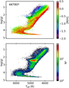 |
Fig. 4 Kiel diagram of the APOGEE DR17 input labels of the training sample (44780 stars) coloured by [M/H] (top) and in density plot fashion (bottom). Our training sample is clearly dominated by giants (77% of the sample has log(g) < 3.5), which is a direct effect of both the APOGEE and Gaia-RVS selection functions. |
3 Convolutional neural network for Gaia-RVS
In the present study, we adopted a hybrid CNN approach that was first successfully applied in Guiglion et al. (2020) with RAVE spectra and Gaia DR2 astrometry and photometry. A complete description of the CNN can be found in Guiglion et al. (2020), Ambrosch et al. (2023), and Nepal et al. (2023). We built our CNN models with the open-source deep learning library Keras (Chollet et al. 2015) using the TENSORFLOW backend (Abadi et al. 2015).
3.1 Convolutional neural network principles
Following our previous works and what has been largely adopted in the community when dealing with stellar parametrisation, we adopted a CNN approach. Convolutional neural networks are well known for being sensitive to spectral features and learning from such features, as well as being less sensitive to radial velocity shifts in the spectra than simple artificial neural networks (see for instance Nepal et al. 2023 and references therein). The CNN allows for the building of a high-dimensional non-linear function that translates spectra plus extra data to stellar labels. The architecture of the CNN we employed is built on the architecture of the CNN developed by Nepal et al. (2023). We note that Nepal et al. (2023) and Ambrosch et al. (2023) extensively improved CNN architectures for spectroscopy compared to Guiglion et al. (2020). We therefore refer the reader to the former two papers for more technical details. We used keras_tuner (O’Malley et al. 2019) to further optimise the CNN architecture and fix the model and training hyperparameters.
The hybrid CNN model developed in this paper consists of three input nodes. The core of our approach consists of Gaia-RVS spectra passed through a block of three 1D convolution layers (with 32, 16, and 8 filters in each convolution block, respectively) that focus on extracting the relevant spectral features sensitive to the stellar labels. The first convolution block has 2401 input neurons, corresponding to 2401 pixels of the RVS spectra (see central node in Fig. 6). After extensive testing, we adopted a kernel size of 8 pixels for each convolution block, larger kernels would not have allowed for the detection of small spectral features. We used 1D Max-Pooling layers (after 1D convolution blocks two and three) that help the network focus on important features, in addition to reducing the number of parameters to fit in the CNN. The output of the third convolution layer was then passed through a block of fully connected layers with 128 neurons.
The second node consists of Gaia DR3 apparent magnitudes G, G_BP, and G_RP together with the parallax serving as four input neurons fully connected to a layer of 32 neurons (see left node in Fig. 6). We adopted LeakyRelu activation functions for the fully connected layers Xu et al. (2015), which are commonly adopted in the community as well as in our previous works.
The third input node consists of XP coefficients passed in the form of 110 input neurons, corresponding to the 110 coefficients, to a fully connected layer with 64 neurons (see right node in Fig. 6).
The outputs of these three fully connected layers were then concatenated (total of 32 + 128 + 64 = 224 neurons), combining the information from all three sources, and passed into three fully connected layers with 128, 32, and 5 neurons each. The last layer with five neurons refers to the output corresponding to the five labels, namely, Teff, log(g), [M/H], [α/M], and [Fe/H]. To facilitate a faster and more efficient convergence of the CNN to the global minimum of the loss function, we scaled the stellar labels to values between zero and one. Additionally, we applied the same scaling procedure to the magnitudes and parallax. In the case of XP coefficients, the 55 BP coefficients were normalised relative to the first BP coefficient (corresponding to 15th magnitude; Andrae et al. 2023b) and then scaled between zero and one. Similarly, we performed the same scaling procedure for the 55 RP coefficients.
We adopted the ReduceLROnPlateau callbacks from Keras in order to reduce the number of training epochs and hence the computation time. In order to prevent overfitting and to stop the training when the loss function of the validation set reached its minimum, we used the early-stop callbacks with a patience of 20.
3.2 Training an ensemble of convolutional neural networks
As the weights and biases of a CNN model are initialised stochastically at the beginning of each training phase, the predicted labels can vary between different models. The training sample is usually split randomly into a training6 set (seen by the CNN at each training epoch) and a validation set (used at each epoch to cross-validate with the training set and optimise the CNN weights). Usually, the splitting of the training sample into training and validation sets is only performed once and frozen to train the CNN. In the present study, we adopted a new approach: We split the training sample into seven different training and validation sets with seven random states (keeping a constant training-validation ratio of 75%). In other words, the CNN experienced seven representations of the training sample so that the whole training sample would pass through the CNN. For each random state, four models were trained, leading to 28 CNN models. The 28 trained CNN models were used to predict labels (28 times) for the whole training sample (44 780 star) and the observed sample (841 300 stars). In a given sample, the labels were averaged over the 28 models, while the standard deviation provided an estimate of the CNN’s internal uncertainties. Such a deep-ensemble CNN approach allowed for a more efficient exploration of the gradient space, which helps with generalising and reduces the variance and bias (Lee et al. 2015; Bialek et al. 2020; Ganaie et al. 2022). Deep ensembles are also more efficient when training on large datasets and improve feature selection.
The CNN models reached their minimum validation loss function typically after 80 epochs. The training time of one model was about 8 min on an Apple M1 Macbook Pro laptop (with a total time of 4 h for the 28 CNN models), and the prediction time was ~0.3 milliseconds per star. In other words, the whole observed sample of 8 × 10⁵ RVS stars took about 4 min to compute (total time of ~2 h for 28 models).
 |
Fig. 5 Correlation matrix of the labels together with photometry (Gaia G, G_BP, and G_RP), parallaxes (p), and S/N. Left: training sample (44 780 stars). Middle: observed sample within training sample limits (644 287 stars). Right: observed sample outside of the training sample limits (197 013 stars). The only parameter not fed to the CNN during training was the S/N. |
3.3 Results of the training
In the left column of Fig. 7, we display 2D histograms of the difference between the CNN-trained labels and (input) APOGEE labels as a function of (input) APOGEE labels for the training sample. The dispersion between the input and output labels is 59 K in Teff, 0.11 K in log(g), 0.07 dex in [M/H] and [Fe/H], and 0.04 dex in [α/M], which is remarkable for RVS spectra. We do not show the [Fe/H] results, as they are almost identical to[M/H] (APOGEE DR17 [M/H] tracks [Fe/H]; Abdurro’uf et al. 2022). For the gravities, no significant systematic offset was detected, and the red clump locus is well reproduced. On the edges of the training sample range, we measured larger residuals (−200 K for Teff > 6200 K, −0.13 dex for [α/M] > +0.35) due to the smaller number of stars in these regions of the training sample. The CNN was able to measure [M/H] well, even if one can see a slight residual trend of about −0.04 dex for [M/H] > −0.5 dex and +0.1/+0.2 dex in the very metal-poor regime ([M/H] < −2, due to a lack of training stars in this region of the parameter space). Overall, the tiny mismatch between the input and output labels tells us that the CNN is not likely to overfit and that the small residuals are likely to come from the fact that we combine spectra (with a different wavelength coverage and resolving power compared to APOGEE), Gaia DR3 photometry, parallaxes, and XP spectra.
We also show how GSP-Spec7 atmospheric parameters and [α/M] (Recio-Blanco et al. 2023) compare to APOGEE for the training sample stars. We adopted GSP-Spec Teff and calibrated log(g), [M/H], and [α/M] from Recio-Blanco et al. (2023). We note that the authors performed basic polynomial calibration of log(g) and [M/H] using external parameters from APOGEE DR17, GALAH DR3, and RAVE DR6, while [α/M] was calibrated using the local galactic abundance trend. We applied the recommended GSP-Spec flags, setting the first 13 digits of flags_gspspec to zero (see Table 2 from Recio-Blanco et al. 2023) and resulting in 2 606 stars in common with our training set. We show comparison plots in the right panels of Fig. 7. Overall, the dispersion is two to three times larger compared to the CNN. One can also see the presence of large outliers in Teff (>1000 K bias) and log(g) (> 1 bias), likely due to the fact that RVS spectra alone present limited resolution and spectral coverage. We elevated the results for the RVS dataset to the level of the APOGEE survey both in terms of precision and accuracy, significantly improving the results from GSP-Spec, which did not use external information as we do with our hybrid CNN. Such sys-tematics in GSP-Spec results were recently reported by Brandner et al. (2023).
3.4 Determination of training sample uncertainties
The internal CNN uncertainty of the stellar labels is given by the standard deviation of the 28 CNN-trained models described in Sect. 3.2. Guiglion et al. (2020) and Nepal et al. (2023) have shown that such an internal model-to-model dispersion may not be representative of the expected uncertainty at a given spectral resolution and may be an underestimate of the true uncertainty. This internal uncertainty may not be representative of the precision of the CNN, as it does not reflect the precision from the input labels. In order to provide more realistic uncertainties, we proceeded as in Nepal et al. (2023). Therefore, in the training sample, we computed the mean dispersion between the APOGEE input and the CNN output labels as a function of the APOGEE input labels. Such a dispersion gives an estimate of the precision with respect to the training sample input labels that are considered as ground truth.
The results are shown in Fig. 8. The internal dispersion over the 28 CNN models (red colourmap) is on the order of 30–40 K in Teff, 0.05 dex in log(g), 0.03/0.05 dex in [M/H] and [Fe/H], and 0.01 dex in [α/M]. The green line in the figure represents the running dispersion of the difference between the CNN output and the APOGEE input labels and shows how the training is precise compared to the ground truth. When quadratically combining the internal dispersion and the running dispersion, the total uncertainty significantly increases (in blue). We note a 50 K uncertainty in Teff for the giants and 60–70 K for the dwarfs. The log(g) is rather constant, around 0.1 dex. The [M/H] and [Fe/H] precision increase from 0.06/0.08 dex in the intermediate metallicity domain to 0.15 dex in the very metal-poor regime, due to the paucity of spectral features. The [α/M] is extremely precise, with a typical precision on the order of 0.02/0.04 dex. We note that such a remarkable precision for all labels at RVS resolution is only achievable when combining external information in the form of Gaia DR3 photometry, parallaxes, and XP coefficients.
 |
Fig. 6 Flow chart of CNN. Gaia-RVS spectra are used as input spectra and passed through the convolution layers for feature extraction. Extra information is fed to the CNN in the form of Gaia DR3 parallaxes as well as G, G_BP, and G_RP photometry (on the left) and XP coefficients (on the right). The information is fully connected (FC) to the output labels Teff, log(g), [M/H], [α/M], and [Fe/H]. |
 |
Fig. 7 Two-dimensional density distribution of the residual between trained CNN labels and APOGEE input labels as a function of the APOGEE input labels for the training sample (44780 stars, left column). The black dashed line shows a null difference. The mean bias (b) and dispersion (σ) of the difference is given in the bottom-left corner of the panels. Each panel also contains a histogram of the input label. The right panels show differences between the calibrated GSP-Spec parameters (with good quality flags; Recio-Blanco et al. 2023) and APOGEE labels. |
3.5 Exploring the convolutional neural network gradients
In this section, we provide a comprehensive view of the features used by the CNN during the training process. We present feature maps for RVS spectra in Sect. 3.5.1 and XP feature maps in Sect. 3.5.2.
3.5.1 RVS gradients
As demonstrated in Nepal et al. (2023), Ambrosch et al. (2023), as well as in Fabbro et al. (2018), CNNs are able to learn each label from specific spectral features. We computed CNN gradients for the training sample RVS spectra by performing partial derivatives of each of the labels with respect to each input neuron (or pixel), namely, δLabel/δλ. Such gradients provide comprehensive maps of the active spectral features during the CNN training. The RVS gradients are shown in Fig. 9. We present mean gradients for the solar [M/H] (solid line) and [M/H] ~ −0.8 dex (dashed line) RC stars. We present some characteristic features used by the CNN that were taken from various literature sources (Boeche et al. 2011; Guiglion et al. 2018; Contursi et al. 2021). Apart from being the strongest feature in the Gaia-RVS range, the CaII triplet is not the most prominent feature in the gradient maps. In the blue wing of the Ca II 8544 line, the Fe I+Ti I blend is active for all labels. We observed that the Cr II line at 8551Å is active for Teff and log(g), but almost no signal is present in [M/H] and [α/M] gradients. An Fe I and Fe I+Ti I blend at ~8520 Å is mainly active in Teff log(g), and [M/H]. A very interesting feature can be seen at λ ~ 8650 Å: a blend of Si I, V II, and N. This blend is mainly active in log(g), [M/H], and [α/M] gradients. The training was done on APOGEE labels for which we knew the APOGEE C and N features correlate with mass (Salaris, Maurizio et al. 2015; Martig et al. 2016) and therefore also with APOGEE metallicity and [α/M]. This explains why the N feature is used by the CNN for constraining log(g), [M/H], and [α/M]. An Fe I blend in the red wing of the Ca II line at 8664 Å seems to be a very relevant feature for the determination of the four labels. We note that most of the spectral features used in the range 8570–8640 Å are composed of Fe I lines. In the red part of the RVS domain, we observed numerous lines contributing to gradients: an SI line is active in Teff and log(g) gradients as well as in Ti I. Such lines are also active in [M/H] and [α/M], but to a lower extent. From what we observed, the CNN learns [α/M] from mainly Si I, Ca II, and Ti I lines and from the blend of Si, V, and N. Overall, the CNN is able to learn from distinct spectral features for a given label even if the resolution is ~ 10 000. This bodes well for the future exploitation of 4MOST low-resolution surveys (Chiappini et al. 2019; Helmi et al. 2019; Cioni et al. 2019).
3.5.2 XP gradients
We investigated how the network learns from the XP coefficients. To that end, we first computed correlations between the labels and the 110 XP coefficients. As presented in Fig. 10, the correlation matrix tells us that some coefficients are more correlated to labels than others. It is evident from the heatmap in the figure that XP spectra contain a lot of information on the stellar atmospheric parameters Teff, log(g), [M/H], and [α/M]. Interestingly, some of the XP coefficients show a good amount of correlation with the alpha abundance as well. We then expected the CNN to learn differently from each XP coefficient. In the same way we did for the RVS spectra, we computed gradients for the 110 XP coefficients. We present the XP gradient (δXP/δlabel) as a function of XP coefficients in the right panel of Fig. 10. The gradients show a lot of activity, meaning that the CNN uses and learns from the XP coefficients for the training sample. The basis functions with high orders in RP (>30) do not seem to show strong activity, meaning that the CNN may learn most from the lower-order coefficients. In case of BP, information is present even down to coefficient 45. The gradients are fairly consistent with the correlations observed between XP and labels. Such plots confirm that XP coefficients are extremely rich in information (see Andrae et al. 2023b; Zhang et al. 2023) and can provide additional constraints when measuring Teff, log(g), [M/H], [Fe/H], and [α/M].
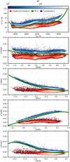 |
Fig. 8 Convolutional neural network uncertainties of the training sample as a function of CNN output labels. The 2D density distribution in the red colourmap corresponds to the internal precision computed over the 28 CNN models. The green fit corresponds to the running dispersion computed from the residual of CNN-APOGEE training labels (see Fig. 7). The 2D histogram in the blue colourmap corresponds to the quadratic sum of the internal precision and running dispersion, and defines our overall uncertainty. |
4 Predicting labels for the observed sample
Using the 28 CNN models, we predicted the atmospheric parameters Teff, log(g), [M/H] as well as [Fe/H] and [α/M] ratios for 841 300 Gaia-RVS stars, that is, the previously defined observed sample together with their uncertainties as detailed in Sect. 3.4. Among these 841 300 stars, we have 644 287 stars within the training sample limits as defined in Table 1 and Sect 5.1.
4.1 Kiel diagrams of the observed sample
In Fig. 5, we show a correlation matrix of labels, photometry, parallaxes, and S/N of the RVS spectra classified as within the training sample limits (middle column). Correlations are consistent with those from the training sample (left column), as expected. On the other hand, when drawing a correlation matrix for the rest of the observed sample (outside the training sample limits), we did not see any strong correlation of Teff with parallaxes. In fact, G and G_RP are anti-correlated with Teff. Such a behaviour is discussed in more detail in Sect. 5.3 and is mainly due to the presence of underrepresented spectral types in the training sample.
In Fig. 11, we show Kiel diagrams of the observed sample in bins of S/N (15–25, 25–35, 35–75, and ≥75) colour-coded with [M/H] (644287 stars). We observed a very consistent Kiel diagram with a clear metallicity sequence in the giant branch. The CNN also does a good job of parameterising the red clump. We note that the CNN catalogue contains 10718 RVS stars with [M/H] < −1. We also observed a secondary cool-dwarf sequence, which is very similar to what has been observed in RAVE DR6 (Steinmetz et al. 2020b) and in which case results from the presence of binary stars. Indeed, these stars in the regime 4600 < Teff < 5100 K and 4 < log(g) < 4.2 show a very large Gaia DR3 RUWE (~4), suggesting a poor astrometric solution likely due to binarity. We further discuss the stability of the CNN with radial velocity errors in Appendix C.
We also present Kiel diagrams for the rest of the RVS sample (197 013 stars) in grey (stars outside the training sample limits). Such stars are discussed in more detail in Sect. 5. In Appendix B, we provide more detail regarding the CNN application using only RVS spectra (i.e. no photometry, parallaxes, or XP data).
In order to show that the CNN is able to properly parame-terise the RVS spectra, we show in Fig. 12 the mean spectra from the observed sample in sequences of Teff, log(g), [M/H], and [α/M] as derived by the CNN. Panel a of the figure shows typical turn-off stars with solar [M/H], ranging from ~4900 to 6000 K. As expected, cooler stars present shallower spectral lines. Next, panel b shows a log(g) sequence from 2.7 to 4.4 dex for stars around 5000 K and solar [M/H]. In the same fashion as Teff, cooler stars present shallower CaII feature, while the Fe I and Ti I blend do not show strong sensitivity to gravity. Panel c shows a metallicity sequence from −1.5 to solar [M/H] for cool giants.
Overall, the more metal-poor stars suffer from the weakening of spectral lines, as expected. Panel d shows a [α/M] sequence for cool dwarfs from Solar to +0.26. Similar to [M/H], shallower lines result from lowering the overall [α/ M] ratio. The Ti I component of the blend seems more sensitive to [α/M] enrichment. Such diagnostic plots show that the CNN properly determines stellar labels and propagates the knowledge from the training sample labels.
 |
Fig. 9 Gaia RVS spectral sensitivity maps of CNN. Top: mean RVS spectra of training sample RC stars with [M/H] ~ 0. In the next sub-panels, we show the mean gradients of the CNN output labels with respect to the input RVS pixels for Teff, log(g), [M/H], and [α/M] (δlabel/δλ). The vertical coloured lines show the location of the main RVS spectral features from which CNN learns (see Sect. 3.5.1). |
4.2 Uncertainties of the observed sample
The uncertainties were derived by quadratically combining the dispersion from the 28 CNN models together with the fit of the running dispersion from the training sample (polynomial curve in Fig. 8). In Fig. 13, we present the total uncertainty of the 768 793 stars within the training sample limits. The bulk of the sample shows very similar uncertainty distributions to those in the training sample (see Fig. 8). Stars with larger uncertainties are also present. For instance, cool super giants show uncertainties on the order of 70–300 K in Teff, 0.15–0.5 dex in log(g), and 0.1–0.3 dex in [M/H] (roughly 19000 stars). We note that we provide to the community both the model-to-model dispersion and the overall combined uncertainty (see Table 2).
4.3 The [α/M] versus [M/H] distributions of the observed sample
We explore in this section the abundance pattern of [α/M] versus [ M/H] of the observed sample in the different regions of the Kiel diagram when selecting stars within the training sample limits (644287 stars).
In Fig. 14, [α/M] versus [M/ H] patterns are presented in bins of 500 K in Teff and 1 dex in log(g). As expected, we probed the low-[α/M] regime preferentially in the dwarf regime, as such objects are likely located closer to the Sun. We started probing the high-[α/ M] sequence when moving to lower log(g), and we started populating the metal-poor tail of the sample. In the region 4000 < Teff < 4500 K and 1 < log(g) < 2, we clearly observed a bimodality in [α/M], as expected (e.g. Hayden et al. 2015; Queiroz et al. 2020). Such a feature was not visible using RAVE data (Guiglion et al. 2020). We discuss the bimodality in more detail in Sect. 7.
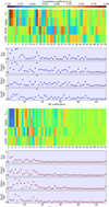 |
Fig. 10 Gaia XP spectra sensitivity maps of CNN. In the top panel, we show a correlation matrix shown as a heat map between the 55 BP XP coefficients and labels in the training sample. The colour bar shows the strength of the (anti-)correlation, where green in the middle (zero value) represents no linear relationship between the labels and XP coefficients. The second panel shows the mean gradients of BP XP coefficients (δlabel/δXP) as a function of the 55 BP XP coefficients for the training sample. The third and fourth panels depict the heat map and gradients for the RP XP coefficients (i.e. the red part of XP spectra). |
4.4 Precision and accuracy of metal-poor stars in the observed sample
We investigated the precision and accuracy of metal-poor stars present in the observed sample that fall within the training sample limits. As a reference, we used APOGEE DR17 labels and focused only on the stars with [M/H]APOGEE < −1.To demonstrate the robustness of the CNN in the low S/N regime, we selected stars with 15 < S / N < 25. We note that GSP-Spec do not provide results with good quality flags_gspspec for these stars. In Fig. 15, we compare the CNN labels to APOGEE DR17 for 353 RVS metal-poor stars of the observed sample. The effective temperature and surface gravity show no significant bias, with a dispersion of 75 K and 0.17 dex, respectively. The overall [M/H] also shows no significant bias, with a dispersion of 0.14 dex. The bottom panel of Fig. 15 shows an [α/M] dispersion below 0.07 dex and a tiny residual that is a function of [α/M] and is consistent with the training sample (see Sect. 3.3).
Taken together, these results demonstrate that the CNN is able to provide robust parameterisation of metal-poor stars down to [M/H] = −2.3 dex at 15 < S /N < 25. Notably, this is the S/N regime where standard spectroscopy struggles to provide precise and accurate measurements for such types of stars.
Atmospheric parameters, chemical abundance ratios, uncertainties, and boundary flag of the publicly available online catalogue of 886080 Gaia-RVS stars.
4.5 Stability of the convolutional neural network in the low signal-to-noise ratio regime
The Gaia DR3 RVS sample contains a significant fraction of low S/N stars: 38% of the observed sample spectra range from 15 to 25 in S/N. In this section, we investigate how the CNN precision varies with the S/N. Thus, we computed the standard deviation between the CNN labels and APOGEE DR17 for stars within the training sample limits in the observed sample. We computed the same quantities in the training sample for reference. In Fig. 16, we show how the precision behaves as a function of the S/N. For the training sample (in orange, solid lines), the CNN precision is extremely stable and constant with respect to the S/N for our four labels (Teff, log(g), [M/H], and [α/M]). As a comparison, the precision of the GSP-Spec with respect to APOGEE is two to five times worse (in orange, dashed lines), showing decreasing precision with a decreasing S/N. We observed the same behaviours in the observed sample (in green). The CNN precision is constant as a function of the S/N in the observed sample as well, which is not the case for GSP-SPec, again due to the fact that the CNN combines spectroscopy, photometry, and astrometry. Such plots show how the CNN is able to efficiently deal with the noise in the data compared to standard spectro-scopic methods, and it is able to extract high-quality labels in low S/N spectra. Such an advantage of the CNN will be key for the next data releases of Gaia, for instance, for extracting information from individual epoch spectra at very low S/N, where epoch spectra will be released at intrinsically lower S/N than the presently available time-averaged spectra. In Appendix C, we present additional CNN sensitivity tests with respect to radial velocity uncertainties.
 |
Fig. 11 Kiel diagrams of 644 287 Gaia-RVS stars in bins of S/N selected within the training sample limits. The stars are colour-coded by metallicity. In the background, we show 2D histograms (in grey) of 197 013 stars that fall outside of the training sample limits. |
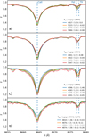 |
Fig. 12 Mean RVS-observed spectra plotted in sequences of Teff (panel a), log(g) (panel b), [M/H] (panel c), and [α/M] (panel d.). We identified the two main spectral features as Ca II and a blend of Fe I and Ti I. |
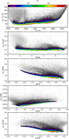 |
Fig. 13 Two-dimensional density distribution of the total uncertainties for the 644 287 observed sample stars within the training sample limits as a function of stellar labels. In the background, we show in grey the uncertainty distributions for stars outside of the training set limits (see Sect. 5). |
 |
Fig. 14 Representation of [α/M] versus [M/H] for 644287 Gaia-RVS stars of the observed sample within the training sample limits. The sample is presented in panels corresponding to cuts in the effective temperature and surface gravity (steps of 500 K in Teff and 1 dex in log(g)). In the top-left corner, we show a Kiel diagram of the sample to guide the eye. |
5 How to ensure that the convolutional neural network labels are within the physical limits of the training set
Machine learning algorithms, such as the CNN, are extremely proficient at learning from spectral features present in a training sample spectra. Nevertheless, some spectra of the observed sample may not share common features with the training sample. Hence, parameterising such types of spectra could lead to systematics in the determined labels. To understand how reliable the CNN labels are, we present in the next sections a classification method based on t-SNE, and we explore in Sect. 5.3 the labels of stars outside of the training limits.
5.1 Using the t-SNE method to understand the limitations of convolutional neural network labels
In order to supplement the reliability of our CNN results, we performed a classification of our observed sample spectra into ‘training-like’ and ‘training-unlike’ spectra, in the same fashion as in Ambrosch et al. (2023). For such a task, we used t-SNE, which is a dimensionality reduction technique (Van der Maaten & Hinton 2008). From an N-dimensional dataset (i.e. full spectra), t-SNE will provide a 2D map where each point corresponds to a data sample, and points close to each other in such a map then share similar spectral features. We concatenated the training sample (44 780 spectra) and the observed sample (841 300 spectra) into a main sample of spectra (886 080 spectra), in all composed of 2401 pixels. We produced four different t-SNE maps with perplexity = [30, 50, 75, 100]. We emphasise that this hyperparameter is equivalent to the number of neighbours for a given data point (see Van der Maaten & Hinton 2008 for more details). We give an example of a t-SNE map with perplexity = 50 for the RVS sample in Fig. 17. Panel a of the figure shows a density map of the 886 080 spectra, colour-coded by the number of spectra per bin. In panel b, we display the same map but highlight the training sample spectra in green and the observed sample spectra in yellow. One can clearly see that in some regions, only yellow points are visible, meaning that such observed spectra do not share the same spectral features as the training sample spectra. We computed geometric distances between each point of the training sample and the observed sample in the t-SNE map for the four different perplexities. We selected observed spectra similar to the training sample simultaneously for the four learning rates (an observed spectrum must be similar to a training sample spectrum in each of the four computed t-SNE maps). A similar method was already used in Ambrosch et al. (2023) for selecting training-like observed spectra. In panel c, we show 669 572 RVS spectra that are training-like, while panel d shows 171 728 training-unlike RVS spectra. In Appendix A, we show similar plots for the four classifications in Fig. A.1 and plots for the classification with perplexity = 75 colour-coded with Teff, log(g), and [M/H] in Fig. A.2.
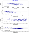 |
Fig. 15 Residual between the CNN and APOGEE parameters as a function of APOGEE for 353 metal-poor stars ([M/H]APOGEE < −1 dex) in the observed sample in the range 15 < S /N < 25. The black dashed line shows a null difference. The mean bias (b) and dispersion (σ) of the difference is given in the bottom-left corner. |
5.2 Defining a robust flag to isolate spurious convolutional neural network labels
Thanks to the t-SNE classification, we were able to isolate the CNN labels that may suffer from systematics. Additionally, Gaia G, parallaxes, and labels of the observed sample outside of the physical limits of the training sample (as described in Table 1) can suffer from systematics. We provide an eight-digit integer flag in which each digit corresponds to one of the labels (in the order Teff, log(g), [M/H], [α/M], and [Fe/H]) as well as the Gaia G magnitude, parallax, and t-SNe classification. For instance, ‘00000000’ means that all labels are within the training sample limits and within the G magnitude and parallax of the training sample and that the t-SNE classification considered this spectrum to be similar to the training set. In contrast, a star with ‘10000000’ would indicate that the Teff derived by the CNN is outside of the training sample limits and should be taken with caution. We note that the flag we provide can be used to search for peculiar stars or non-FGK objects in the RVS sample.
5.3 Exploring the labels outside of the training sample limits
In this section, we present the CNN labels of the 197 013 observed sample stars outside the limits presented in Table 1 and classified by t-SNE as training-unlike (i.e. flag≠00000000). The sample consists of 197 013 stars, and Kiel diagrams are presented in Fig. 18. The sample seems to cover a large range of [M/H] from −3 to +1.
The typical spectrum of the giant branch is presented in the bottom-right corner of each panel in Fig. 18. It shows very strong TiO bands that increase with metallicity. As a result, the CNN interprets the strong TiO bands as metal-rich features. Labels for these stars are unlikely to be accurate. Such TiO bands indicate that such stars are M giants (confirmed by their Gaia DR3 spectraltype_esphs). Such stars were also observed in RAVE (Matijevič et al. 2012). There are no such stars in the training set.
In the top-left corner of each panel of Fig. 18, we show spectra of the hot stars. The spectra show very strong Hydrogen Paschen lines, in fact indicating very hot stars. The strength of the Paschen lines decrease with increasing metallicity, indicating that the CNN understands the Paschen lines as being metal-poor lines. These spectra are classified as OB stars when checking the spectraltype_esphs from Gaia DR3. The CNN labels are also unlikely to be accurate.
With Fig. 19, we investigated in more detail three regions of the Kiel diagram that present labels for both the CNN and APOGEE DR17: hot dwarfs (5700 ≤ Teff ≤ 7000, 2 ≤ log(g) ≤ 4.5; blue dots), cool dwarfs (4000 ≤ Teff ≤ 5000, log(g) ≥ 4.5; green crosses), and cool giants (2000 ≤ Teff ≤ 4800, −2 ≤ log(g) ≤ 2; orange stars). Regarding the hot dwarfs, we clearly observed that for Teff > 7000 K, there is a large discrepancy between the CNN labels and APOGEE directly accountable for the large Paschen features in the RVS spectra and caused by the fact that the training sample does not contain such targets. The gravity suffers from large systematics as well, while [M/H] and [α/M] match rather well within 0.12 and 0.05 dex, respectively.
Concerning the cool dwarfs, the main issue comes from a poorly parameterised log(g), as such objects are very nearby with parallaxes larger than 7 mas. In the current training sample, we have few nearby cool dwarfs. Hence, the CNN gravities for such objects strongly suffer from systematics.
Finally, we observed that the cool giants show discrepant Teff up to +1000 K compared to APOGEE, with metallicity systematics up to +1 dex. Surprisingly, the [α/M] agrees within 0.1 dex between APOGEE and the CNN.
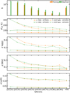 |
Fig. 16 Precision computed as the standard deviation of the CNN minus APOGEE (solid lines) and calibrated GSP-Spec minus APOGEE (dashed lines) as a function of S/N bins for 41 623 stars of the training sample (orange) and 76 996 stars of the observed sample (green, within the training sample limits). |
 |
Fig. 17 Classification of Gaia RVS spectra with t-SNE. Panel a: t-SNE maps with perplexity = 50 of the entire RVS sample consisting of 886080 spectra plotted in a 2D-histogram manner. Panel b: same map but split into training (green) and observed (yellow) samples. Panel c: spectra of the observed sample identified as similar to that of the training sample. Panel d: spectra of the observed sample identified as not being similar to that of the training sample. See Sect. 5 for more details. |
 |
Fig. 18 RVS stars outside of the training sample limits. The Kiel diagram representations (197 013 stars) are in bins of [M/H] and colour-coded as a function of [M/H]. We show typical RVS spectra of different regions of the Kiel diagram. |
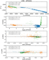 |
Fig. 19 Stars outside of the training set limits. The residual of the CNN minus APOGEE for hot dwarfs, cool giants, and cool dwarfs were selected from Fig. 18 (see text for more details). |
5.4 The catalogue of RVS labels with convolutional neural network
We present our catalogue of atmospheric parameters (Teff, log(g) and [M/H]) along with chemical abundances ([Fe/H], [α/M]) for 886080 Gaia-RVS stars (summarised in Table 2). We provide two sources of uncertainties, model-to-model uncertainties (eTeff, elog(g), e[M/H], e[Fe/H], and e[α/M]) and overall combined uncertainties (σTeff, σlog(g), σ[M/H], σ[Fe/H], and σ[α/M]), as well as the eight-digit flag described in Sect. 5.2. The data table is publicly available with the AIP Gaia archive8. The CNN Python code can be provided upon reasonable request. In order to use the CNN catalogue of labels, we recommend using the eight digits to identify the stars within the training sample limits, that is, the stars with the best CNN parameteri-sation. To select the CNN labels within the training set limits, we recommend adopting flag_boundary = “00000000”.
 |
Fig. 20 Atmospheric parameter comparison between CNN and APOGEE (left column), GSP-Phot and APOGEE (middle column), and GSP-Phot and CNN (right column) for 33 120 stars of the observed sample. |
6 Validation of convolutional neural network labels
We validate our CNN methodology in his section. We used external datasets in the form of asteroseismic data, parameters from GSP-Phot, and GALAH data.
6.1 Comparison of convolutional neural network labels with GSP-Phot
In this section, we compare the CNN labels of the observed sample with atmospheric parameters from GSP-Phot (Andrae et al. 2023a). We note that Gaia DR3 provided the community with spectro-photometric atmospheric parameters using parallaxes, stellar magnitude, and BP and RP coefficients.
In Fig. 20, we present comparisons between the CNN and GSP-Phot9 with respect to APOGEE, as APOGEE was used as training labels. We required that the CNN labels be within the training set limits, resulting in having 33 120 labels in common between APOGEE, the CNN, and GSP-Phot. The left columns of Fig. 20 show a comparison of the CNN labels to APOGEE, and a very similar behaviour as seen in Fig. 7 can be observed. When comparing GSP-Phot with APOGEE (middle column of Fig. 20), a larger overall dispersion can be measured, two to three times larger than when comparing the CNN to APOGEE. There are significant systematics for Teff < 4500 K and log(g) < 2. We also noticed a double sequence in the [M/H] residual for [M/H] > −0.8. The most striking feature is the large residual trend for [M/H] < −0.8, with a difference larger than 0.5 dex. The third panel of Fig. 7 presents comparisons between the CNN and GSP-Phot. Overall, the dwarfs compare quite well, while the giants show rather large discrepancies in both Teff and log(g), consistent with what is shown in the left and middle panels of Fig. 7. The large discrepancy in the parameters between CNN and GSP-Phot can be explained by the fact that the CNN combines RVS spectra, astrometry, photometry, and BP and RP coefficients and that it trains on labels from the high-resolution APOGEE survey.
6.2 Validation of surface gravities with asteroseismic data
To test CNN accuracy and precision in surface gravity, we compared the CNN log(g) with the precise log(g) from astero-seismology. Asteroseismology relies on stellar oscillations and is widely used by spectroscopic surveys for validation or calibration purposes, such as in RAVE (Valentini et al. 2017), Gaia-ESO (Worley et al. 2020), and APOGEE (Anders et al. 2017; Pinsonneault et al. 2018; Miglio et al. 2021). For stars with solar-like oscillations, as well as red giants, the frequency at maximum oscillation power (vmax) is used for determining log(g)seismo using only the additional parameter Teff (Brown 1991; Kjeldsen & Bedding 1995; Chaplin & Miglio 2013). We adopted the most recent version of the K2 Galactic Archaeology Program (K2 GAP) for campaigns C1-C8 and C10-C18 from Zinn et al. (2022). The authors provide asteroseismic parameters for 19000 red giant stars. We have 164 stars in common with our training sample and 589 stars in common with our observed set (within the training sample limits). Each star also has GSP-Spec calibrated log(g) for further comparison, with the 13 first flags_gspec equal to zero. We computed log(g)seismo from Zinn’s vmax and Teff using Eq. (3) from Valentini et al. (2019), assuming vmax,⊙ = 3090 µHz and Teff,⊙ = 5777 K (Huber et al. 2011).
In Fig. 21, we present a one-to-one comparison between the asteroseismic log(g)s and APOGEE DR17, CNN, and GSP-Spec surface gravities in the training and observed samples. Firstly, the APOGEE and seismic log(g) compare very well in both the training (used as input labels) and observed stars. No significant bias was measured, while the dispersion ranges from 0.05 to 0.07, depending on the log(g) range. This absence of bias is consistent with the fact that APOGEE calibrated the spectroscopic log(g) with respect to the seismic ones (Abdurro’uf et al. 2022). Secondly, the CNN and seismic log(g) also compare very well, with no significant bias for log(g) < 2.6. For log(g) > 2.6, we measured a small bias on the order of 0.1 dex in both training and observed stars, likely due to the fact that we combined spectra, photometry, parallaxes, and XP coefficients. In the observed sample, the dispersion ranges from 0.04 to 0.09 dex, which is remarkable. The red clump (in green) shows no apparent bias as well as a dispersion below 0.1 dex. We note that the log(g) residual between APOGEE and the CNN shows no trend with respect to the CNN Teff or [M/H]. The CNN is then capable of conserving the APOGEE calibration. Finally, we compared the GSP-Spec-calibrated log(g) with respect to the seismic log(g). We observed that the calibrated GSP-Spec gravities match quite well the seismic log(g), with a dispersion on the order of 0.15, while biases range from 0.10 to 0.11.
Such comparisons once again show the remarkable performances of the CNN, which combines several datasets for improved measurements compared to pure spectroscopic labels (as derived by GSP-Spec). The CNN is able to transfer and preserve the properties of the training set, which in the present case refers to the seismic calibration of APOGEE labels. (We refer the reader to Appendix B for a CNN application using RVS spectra only.)
 |
Fig. 21 One-to-one comparisons of surface gravities log(g) from APOGEE DR17 (left column), CNN (middle column), and calibrated GSP-Spec (right column) with respect to seismic log(g) calculated based on vmax and Teff from Zinn et al. (2022). The top row shows stars of the training sample, while the bottom row shows targets of the observed sample. We computed the mean bias (b) and mean dispersion (σ) for three ranges of gravity: log(g) < 2.3 (orange), 2.3 < log(g) < 2.6 (green), and log(g) < 2.6 (red). |
6.3 Comparison between convolutional neural network and GALAH DR3
We previously assessed CNN performances with respect to APOGEE (which could reflect our training sample) and GSP-Spec (which uses the same spectra as the CNN). In order to have a fully independent comparison, we adopted the third data release (DR3) of the high-resolution (R ~ 28 000) optical spectroscopic survey GALAH (Buder et al. 2021). GALAH DR3 used the Spectroscopy Made Easy (SME; Valenti & Piskunov 1996) spectral fitting code to derive atmospheric parameters and chemical abundances for 588 571 stars. We adopted GALAH quality flags according to the recommendations presented in the best practices for using GALAH DR310, including removing stars flagged to have peculiarities in their stellar parameters and iron and alpha abundances, namely, flag_guess = 0, flag_sp = 0, flag_fe_h = 0, flag_alpha_fe = 0, and we made a S/N cut with snr_c3_iraf > 40 per pixel. Regarding CNN labels, we only required that labels be within the training sample limits. For completeness, we also compared GALAH to calibrated GSP-Spec parameters. Following the above selection, the sample consisted of 24 803 stars in common between the CNN and GALAH DR3 and with labels within the training sample limits and 15 ≤ S /N ≤ 25.
In Fig. 22, we present label differences in the form CNN -GALAH as a function of GALAH. We observed that Teff and log(g) present no strong systematics, apart from hot dwarf stars (Teff > 6500 K) with a significant bias of >300 K (total of 200 stars). For gravities, log(g) shows a weak residual trend with a dispersion on the order of 0.1. We note that such a dispersion increases to 0.17 for log(g) < 2.2. The CNN [M/H] shows remarkable agreement with GALAH, with a dispersion below 0.1 for [M/H] > −1, and it reaches 0.19 dex for [M/H] < −1. In addition, the CNN [α/M] matches GALAH well, with a dispersion well below 0.1. We note that the systematic trends measured between the CNN and GALAH are also visible in the input APOGEE DR17 labels. In this section, we have demonstrated that the CNN parameters in the range 15 ≤ S /N ≤ 25 based on spectroscopy, astrometry, and photometry are very consistent with high-resolution spectroscopic GALAH parameters.
 |
Fig. 22 Differences between CNN minus GALAH as a function of GALAH for Teff, log(g), [Fe/H], and [α/M] for 24 803 stars of the observed set with 15 ≤ S /N ≤ 25 and within the training set limits. |
6.4 Comparison of convolutional neural network iron content with open clusters from GALAH
We compare here the CNN [Fe/H] predictions for open cluster stars to those from GALAH DR3. We used a list of known clusters within the Gaia-RVS clusters from Cantat-Gaudin et al. (2020) updated to DR3 (Cantat-Gaudin, priv. comm.). There are nine clusters with more than three members ranging from −0.4 to +0.25 in [Fe/H]. We present a comparison plot in Fig. 23. Overall, the CNN [Fe/H] agrees very well with GALAH. However, two clusters present rather large systematics. For instance, NGC 2539 shows a mean difference of 0.26 dex between the CNN and GALAH. A recent study by Casamiquela et al. (2021) found this cluster to be slightly sub-solar ([Fe/H] = −0.012), which is consistent with the CNN data. The second cluster, NGC 2632, shows a rather large dispersion of 0.12 dex for GALAH [Fe/H], while the CNN finds an internal dispersion of 0.05 dex. The mean [Fe/H] abundance is 0.08 for the CNN and 0.19 for GALAH, while Casamiquela et al. (2021) reported 0.12 as the mean [Fe/H]. Our comparison plot allowed us to show the robustness of the CNN [Fe/H] ratios.
 |
Fig. 23 Comparison of CNN [Fe/H] with respect to GALAH DR3 for 10 open clusters. The clusters are listed in the top-left corner. We also computed a mean [Fe/H] and the associated error bar (computed as standard deviation). The mean bias is written next to the cluster name. |
7 The [α/M] – [M/H] bimodality traced by Gaia-RVS
The abundance patterns of α-elements (such as magnesium and oxygen) have been studied and characterised in the Milky Way disc, bulge, and halo for more than two decades in the solar neighbourhood (e.g. Fuhrmann 1998, 2011; Pompéia et al. 2002; Adibekyan et al. 2011; Mikolaitis et al. 2014; Guiglion et al. 2015) and toward the inner and outer disc thanks to large-scale spectroscopic surveys (e.g. Anders et al. 2014; Hayden et al. 2015; Buder et al. 2019; Queiroz et al. 2020). A strong debate has animated the Galactic Archaeology community regarding the mechanisms responsible for the bimodality measure in this abundance space (see for instance Chiappini et al. 1997; Schönrich & Binney 2009; Haywood et al. 2013; Minchev et al. 2013; Grand et al. 2018; Spitoni et al. 2019; Buck 2020; Khoperskov et al. 2021; Agertz et al. 2021). So far, the bimodal-ity has been clearly characterised at high resolution, even though hints of such a bimodality have been detected by low-resolution and intermediate-resolution surveys, such as SEGUE (Lee et al. 2011), LAMOST (Xiang et al. 2019), and RAVE (Guiglion et al. 2020). We have shown in the previous sections that our CNN methodology provides precise and accurate chemical information. In Fig. 4.3, we presented that giant stars show a bimodality in the [α/M] – [M/H] plane, and this is the first time that such a clear bimodality has been seen in Gaia-RVS spectra, which are characterised by both limited resolution and spectral coverage. Our finding is fully consistent with previous work: a low [α/M] sequence (< +0.15 dex) ranging from [M/H] ∼ −0.6 to [M/H] ~ +0.2 dex together with a high [α/M] (> +0.15 dex) sequence ranging from [M/H] ~ −1 to [M/H] ~ −0.2 dex. We note that in the literature, the shape and zero-point of the bimodality depend on the type of stars used and the type of α-elements studied.
To trace the spatial variations of the bimodality, we calculated the positions and velocities in the galactocentric rest-frame using available astrometric solutions (sky positions and proper motions) and radial velocities from Gaia DR3 (Gaia Collaboration 2023) and assuming distances computed with the StarHorse Bayesian method (Queiroz et al. 2023) and the current CNN labels (more details in Nepal et al., in prep.). We also assumed an in-plane distance of the Sun from the Galactic centre of 8.19 kpc (GRAVITY Collaboration 2018), a velocity of the Local Standard of Rest of 240 km s−1 (Reid et al. 2014), and a peculiar velocity of the Sun with respect to the local standard of rest, U⊙ = 11.1 km s−1, υ⊙= 12.24 km s−1, W⊙ = 7.25 km s−1 (Schönrich et al. 2010).
We explored the [α/M] - [M/H] bimodality for 15 ≤ S /N ≤ 25, that is, the S/N regime for which GSP-Spec does not provide [α/M] ratios with good quality flags. In Fig. 24, we show the [α/M] - [M/H] plane decomposed into bins of galactocen-tric radius R and height above the Galactic plane Z. Our sample consists of 53 200 stars with 15 ≤ S /N ≤ 25 and log(g) < 2.3, within the training sample limits. At low Z (IZI < 0.5 kpc) and ± 1kpc around the solar radius, we mainly probed low-[α/M] stars. When moving towards the inner disc, we started to populate the high-[α/M] sequence, and a bimodality is clearly visible in the range 0 < R < 4 kpc (bottom-left panel of Fig. 24). Moving to higher Z (|Z| > 1.0 kpc), the inner disc shows a clear transition from being low-[α/M] populated to high-[α/M] populated (stars in the bins 0 < R < 4kpc and 1 .5 < |Z| < 4kpc; top-left panels of Fig. 24). In the outer disc, the stars mainly show low-[α/M] enrichment, which is due to disc flaring, as first suggested by Minchev et al. (2015). Such results are consistent with previous works (Anders et al. 2014; Hayden et al. 2015). The bimodality is also seen in the bulge region with our CNN abundances, confirming previous results based on APOGEE DR14 and DR16 (Rojas-Arriagada et al. 2019; Queiroz et al. 2020, 2021). By investigating the [α/M] versus [M/H] pattern over a large range of galactic R and Z, we show that CNN is able to recover the main abundance trends in the Milky Way over a large galactic volume, even for low S/N ratio RVS data. This first detection of the bimodality in the RVS data using a CNN is a step forward in the scientific output of the Gaia mission. A detailed discussion of the candidate-bulge stars seen in this sample will be discussed in Nepal et al. (in prep). Other interesting results will also be discussed in forthcoming papers using the new StarHorse method run on this sample (Nepal et al. 2024).
 |
Fig. 24 Two-dimensional histograms and contours of [α/M] vs. [M/H] in 53 200 Gaia-RVS giants of the observed sample with 15 ≤ S /N ≤ 25 and log(g) ≤ 2.2 within the training sample limits. The stars are plotted in kiloparsec bins of galactocentric radius (R) and height above the galactic plane (Z). |
8 Caveats
Stars with [M/H] below −2.3 may suffer from systematics due to low statistics in the training sample at very low metallicities. For the future use of the CNN and Gaia-RVS, a proactive training sample should be adopted by further populating the metal-poor regime. We are going in such a direction with an accepted SDSS-V open-fiber programme (PI G. Guiglion) that will observe 4000 RAVE metal-poor stars (Matijevič et al. 2017; Guiglion et al. 2020) with the APOGEE spectrograph. In the future, such metal-poor stars will complement the current training sample and improve the reliability of the metallicity measurements of stars below −2.3 dex.
Over the full RVS catalogue of 886080 stars parameterised by the CNN, 22% belong outside of the training sample limits. It is clear that in the present study, the performances of our CNN approach are limited by the training sample. The APOGEE and Gaia surveys are characterised by different selection functions. The selection function of the training sample is then characterised by traits common to both surveys, but a full analysis of the selection function is beyond the scope of the present paper. For future Gaia releases, substantial effort should be applied to populating the training sample with more diverse targets, such as OB stars, M dwarfs, and giants. Also, nearby stars (with large parallaxes) or bright stars should be added in the training set in order to have a more complete representation of the local stellar populations. Such statements are valid for ongoing and future large spectroscopic surveys that may want to use ML algorithms for spectral parameterisation, such as GALAH, SDSS-V, and 4MOST.
9 Conclusion
In June 2022, the Gaia consortium released data of one million RVS stars, with one-third having a low signal-to-noise ratio (15 < S /N < 25). In this paper, we derived atmospheric parameters and chemical abundances from this dataset by combining, for the first time, Gaia-RVS spectra, photometry (G, G_BP, G_RP), parallaxes, and Gaia XP coefficients. We summarise our method and main achievements below:
Benefitting from the last data release of the APOGEE survey, we built a training sample with high-quality labels, including atmospheric parameters Teff, log(g), and [M/H] and chemical abundances [Fe/H] and [α/M]. After careful use of Gaia and APOGEE flags, the resulting training sample was composed of 44 780 stars (Sect. 2, Fig. 4) with RVS spectra, photometry, astrometry, and XP data. We also assembled a set of RVS spectra (with additional photometry, astrometry, and XP data) for which we measured the above-mentioned labels. This observed set is composed of 841 300 stars.
We built a CNN based on previously used architectures from Guiglion et al. (2020); Nepal et al. (2023); Ambrosch et al. (2023) that we optimised for the Gaia datasets used in this work (Sect. 3, Fig. 6). We trained a series of 28 CNN models that we combined in order to determine average labels. We showed that the CNN learns from relevant spectral features for a given label as well as from XP coefficients (Sect. 3.5, Figs. 9, and 10). We confirmed that XP coefficients can be used for constraining atmospheric parameters as well as [α/M].
We derived realistic uncertainties by combining the model-to-model dispersion with the departure from the training sample input labels (Sect. 3.4, Fig. 8). The uncertainties in the observed sample are on the order of 50–70 K in Teff; 0.1 dex in log(g); 0.07/0.15 dex in [M/H] and [Fe/H]; and 0.02/0.04 in [α/M].
The CNN shows a stable performance across a large range of S/N (Sect. 4.5, Fig. 16). The dispersion with respect to APOGEE is constant with S/N in both training and observed samples and more robust than the GSP-Spec parameters when compared to APOGEE. We demonstrated that the CNN is capable of precisely and accurately parameterising metal-poor stars in the range 15 < S /N < 25 (see Sect. 4.4, and Fig. 15). Such high-quality parameterisation is only achievable when combining spectra, photometry, parallaxes, and XP data.
Compared with the precise asteroseismic log(g) of red giant stars computed using asteroseismic parameters from Zinn et al. (2022), the CNN shows no mean bias or residual trends, with a typical dispersion of 0.1 dex, which is remarkable (Sect. 6.2, Fig. 21). Such a precision can only be achieved thanks to the external data we used in the form of photometry, parallaxes, and XP coefficients. Comparisons with GALAH DR3 also showed the CNN to have a higher precision compared to GSP-Spec (Fig. 22). We also showed that CNN is very robust regarding radial velocity uncertainties (Fig. C.1).
Using the dimensionality-reduction algorithm t-SNE, we classified the RVS spectra into training-like and training-unlike spectra, allowing us to discard RVS spectra that are not similar to the training sample. As a result, among the 841 300 RVS stars of the observed sample, 644287 stars (including 10718 metal-poor stars) are within the training sample limits and characterised by flag_boundary = “00000000”, and they are recommended for science applications.
With our dataset, it is possible, for the first time, to resolve and trace the [α/M]-[M/H] bimodality in the Milky Way disc using Gaia data (Sect. 7, Fig. 24). Such a performance has been achieved thanks to a large-enough and high-quality training sample combined with a complex CNN architecture, and most important is the combining of four unique datasets (RVS spectra, photometry, parallaxes, and XP coefficients).
As RVS spectra are rich in spectral lines, we plan to measure more elemental abundances for the next releases of Gaia-RVS data, such as Ti, Si, and Ce. In addition, the next Gaia data release will consist of 66 months of data (expected by the end of 2025) and will include all epoch and transit data for all sources (i.e. low S/N RVS data). This current paper represents a step forward in the analysis of such a dataset. For the next studies and generation of surveys, the training sample should be built in a proactive way, that is, by selecting targets to be observed instead of simply using an existing set of reference stars. In this way, the biases inherent to any training sample will be limited. For instance, focus should be on the tail of metal-poor stars as well as bright stars, local stars, and M giants. Such a challenge will have to be faced by 4MOST, which aims at using ML tools for stellar parameterisation. On that topic, we believe that the experience gained here with the analysis of spectra with limited resolution and spectral coverage will be crucial in the development of a CNN method for future surveys, such as the 4MOST Milky Way Disc and Bulge Low-Resolution Survey (4MIDABLE-LR; Chiappini et al. 2019).
Acknowledgements
G.G. sincerely thanks Gal Matijevič for the great time spent in Innsbruck where at least 40% of this paper was written. G.G. is grateful to Rene Andrae for the fruitful discussions during the MPIA Galaxy & Cosmology Retreat 2023. G.G. thanks Tristan Cantat-Gaudin for providing the list of open cluster members within the Gaia-RVS sample. The authors acknowledge the anonymous referee for the comments and suggestions that improved the readability of the paper. G.G. acknowledges support by Deutsche Forschungs-gemeinschaft (DFG, German Research Foundation) -project-IDs: eBer-22-59652 (GU 2240/1-1 “Galactic Archaeology with Convolutional Neural-Networks: Realising the potential of Gaia and 4MOST”). G.G. and S.N. thank the SOC and LOC of the conference “The Milky Way Revealed by Gaia: The Next Frontier” (5–7 Sept. 2023) where results of this paper where presented. We thank the E-science & IT team for COLAB service and research infrastructure at AIP. S.N. thanks the members of the StarHorse team, Chemodynamical group and MWLV & DGGH sections at AIP for lively discussions. We acknowledge the International Space Science Institute for supporting the ISSI team 542 on “CatS - A reference catalogue for Spectroscopic surveys” led by G. Guiglion and M. Valentini, in which this paper was partly designed. M.B. is supported through the Lise Meitner grant from the Max Planck Society. C.C. acknowledges Fundacion Jesus Serra for its great support during her visit to IAC, Spain, during which part of this work was written. We acknowledge support by the Collaborative Research Centre SFB 881 (projects A5, A10), Heidelberg University, of the Deutsche Forschungsgemeinschaft (DFG, German Research Foundation) and by the European Research Council (ERC) under the European Union’s Horizon 2020 research and innovation programme (grant agreement 949173). G.T. acknowledges financial support from the Slovenian Research Agency (research core funding No. P1-0188). J.M. acknowledges support from the ERC Consolidator Grant funding scheme (project ASTEROCHRONOMETRY, https://www.asterochronometry.eu, G.A. n. 772293). This work has made use of data from the European Space Agency (ESA) mission Gaia (https://www.cosmos.esa.int/gaia), processed by the Gaia Data Processing and Analysis Consortium (DPAC, https://www.cosmos.esa.int/web/gaia/dpac/consortium). Funding for the DPAC has been provided by national institutions, in particular the institutions participating in the Gaia Multilateral Agreement. This work made use of overleaf (https://www.overleaf.com/), and of the following PYTHON packages (not previously mentioned): MATPLOTLIB (Hunter 2007), SCIKIT-LEARN (Pedregosa et al. 2011), NUMPY (Harris et al. 2020), PANDAS (McKinney 2010), SEABORN (Waskom 2021). This work also benefited from TOPCAT (Taylor 2005).
Appendix A Details on t-SNe classification
We present here a comprehensive view of the t-SNE classification of RVS spectra for four different perplexities: 30, 50, 75, 100. Results are shown in Fig. A.1. Overall, the t-SNE look visually similar, with quite consistent numbers of ‘training-like’ and ‘training-unlike’ spectra from the observed sample.
To give the reader an idea of how the t-SNE classification correlates with atmospheric parameters, we present in Fig. A.2 the t-SNE classification with perplexity=50 colour-coded with Teff, log(g), and [M/H]. One can clearly see in the ‘training-unlike’ map blobs of cool and hot stars that are not present in the ‘training-like’ map. Such blobs correspond to the cool giants and hot dwarfs described in Section 5.3 and were clearly mislabelled by the CNN. Using this t-SNE approach allows us to adequately flag the mislabelled spectra and then provide the user a robust flag for cleaning the CNN catalogue of spurious measurements.
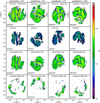 |
Fig. A.1 t-SNE maps of the RVS spectra for four different perplexities (4 columns: 30, 50, 75, 100). The top row shows the maps for the whole RVS sample; the second shows only the RVS classification for the training sample; and the third and fourth rows show the ‘training-like’ and ‘training-unlike’ spectra from the observed sample, respectively. |
 |
Fig. A.2 t-SNE maps for perplexity=5O for the training sample spectra (left) and the ‘training-like’ (middle) and ‘training-unlike’ (right) spectra of the observed sample. The maps are colour-coded with Teff (top), log(g) (centre), and [M/H] (bottom). |
Appendix B Training convolutional neural network of purely Gaia-RVS spectra
We have demonstrated in the previous sections that combining RVS spectra, magnitudes, parallaxes, and XP coefficients allowed us to provide high-quality CNN labels. For completeness, we trained CNN using only RVS spectra as input data. In Fig. B.1, we show Kiel diagrams of the high-quality sample in bins of S/N (15–25, 25–35, 35–75, and ≥ 75), colour-coded with [M/H] (219 145 stars within training set limits. We present the rest of the RVS sample in grey (stars outside the training sample limits or with large uncertainties). We observed a consistent Kiel diagram, even at low S/N, with a clear metallic-ity sequence in the giant branch, while the red clump locus is clearly reproduced. The sequence of cool dwarfs only extends down to Teff = 5000 K, contrary to Fig. 11. This is due to the fact that, similar to RAVE spectra, RVS seems to suffer from degeneracies as well. Such degeneracies are clearly brought to light by the stars in grey, that is, a sequence connecting the cool giants to the cool dwarfs (see Kordopatis et al. 2013; Guiglion et al. 2020 for more details of the RAVE spectral degeneracies). Another interesting feature is a high concentration of stars above Teff > 6500 K. Their spectra are characterised by strong Hydrogen Paschen lines. The CNN seems to constrain their temperature rather well, while log(g) is clearly biased.
In Fig. B.2, we compare CNN gravities (derived from RVS spectra only) to seismic gravities computed from Zinn et al. (2022) (see Sect. 6.2; same stars as in Fig. 21). Overall, the bias is well below 0.1 dex, while the dispersion ranges from 0.08 to 0.12 dex, which is remarkable considering that we only trained on RVS spectra. We emphasise that calibrated GSP-Spec gravities only showed a precision of 0.14–0.17 dex compared to seismic gravities.
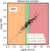 |
Fig. B.2 Same figure as Fig. 21 but comparing the CNN gravities (derived using only RVS spectra) and seismic gravities. |
Through such tests, we show that the CNN still provides reliable parameters when trained only on RVS spectra. This is due to the high-quality APOGEE labels transferred and learned during the training process. The CNN is still not immune to spectral degeneracies for some stars. Such degeneracies are broken when using extra magnitudes, parallaxes, and XP data.
Appendix C Convolutional neural network stability with respect to Gaia DR3 radial velocities
In this section, we investigate how sensitive the CNN is to the radial velocity uncertainties. In this study, the adopted Gaia-RVS have been corrected from Doppler shift by the Gaia consortium. It may happen that a tiny residual shift (a fraction of a pixel) can be present in the corrected spectra of stars with large Vrad uncertainties. We note that small systematics in the radial velocity applied to spectra may lead to systematics in the predicted labels (see Nepal et al. 2023). In Fig. C.1, we show how the difference in labels between CNN and APOGEE and GSP-Spec and APOGEE (in both training and observed samples) varies with Gaia DR3 radial velocity uncertainties (eVrad). We applied the recommended flags_gspspec in order to clean the GSP-Spec sample. First, for the training sample, we clearly observed that for each label (Teff, log(g), [M/H], and [α/M]), the systemat-ics (bias) between CNN and APOGEE is constant as a function of eVrad. On the other hand, GSP-Spec - APOGEE shows strong residual trends for the bulk of the distribution, with increasing bias as a function of eVrad, as documented in Recio-Blanco et al. (2023). The dispersion is also two to three times larger compared to the CNN. For the stars on the observed sample, we observed similar systematic trends. We note that even if not plotted here, [Fe/H] behaves similarly as [M/H]. With such tests, we can conclude that the CNN shows no strong sensitivity to eVrad and shows no residual trends.
 |
Fig. C.1 Two-dimensional density distribution of the CNN minus APOGEE and calibrated GSP-Spec minus APOGEE as a function of Gaia DR3 radial velocity uncertainties in both the training (2 606 stars) and observed samples (20 948 stars, within the training sample limits). |
References
- Abadi, M., Agarwal, A., Barham, P., et al. 2015, TensorFlow: Large-Scale Machine Learning on Heterogeneous Systems, software available from tensorflow.org [Google Scholar]
- Abdurro’uf, Accetta, K., Aerts, C., et al. 2022, ApJS, 259, 35 [NASA ADS] [CrossRef] [Google Scholar]
- Adibekyan, V. Z., Santos, N. C., Sousa, S. G., & Israelian, G. 2011, A & A, 535, L11 [NASA ADS] [CrossRef] [EDP Sciences] [Google Scholar]
- Agertz, O., Renaud, F., Feltzing, S., et al. 2021, MNRAS, 503, 5826 [NASA ADS] [CrossRef] [Google Scholar]
- Ahumada, R., Allende Prieto, C., Almeida, A., et al. 2020, ApJS, 249, 3 [NASA ADS] [CrossRef] [Google Scholar]
- Ambrosch, M., Guiglion, G., Mikolaitis, Š., et al. 2023, A & A, 672, A46 [NASA ADS] [CrossRef] [EDP Sciences] [Google Scholar]
- Anders, F., Chiappini, C., Santiago, B. X., et al. 2014, A & A, 564, A115 [NASA ADS] [CrossRef] [EDP Sciences] [Google Scholar]
- Anders, F., Chiappini, C., Rodrigues, T. S., et al. 2017, A & A, 597, A30 [NASA ADS] [CrossRef] [EDP Sciences] [Google Scholar]
- Anders, F., Chiappini, C., Santiago, B. X., et al. 2018, A & A, 619, A125 [NASA ADS] [CrossRef] [EDP Sciences] [Google Scholar]
- Andrae, R., Fouesneau, M., Sordo, R., et al. 2023a, A & A, 674, A27 [NASA ADS] [CrossRef] [EDP Sciences] [Google Scholar]
- Andrae, R., Rix, H.-W., & Chandra, V. 2023b, ApJS, 267, 8 [NASA ADS] [CrossRef] [Google Scholar]
- Bailer-Jones, C. A. L., Irwin, M., Gilmore, G., & von Hippel, T. 1997, MNRAS, 292, 157 [NASA ADS] [Google Scholar]
- Bensby, T., Bergemann, M., Rybizki, J., et al. 2019, The Messenger, 175, 35 [NASA ADS] [Google Scholar]
- Bergemann, M., Lind, K., Collet, R., Magic, Z., & Asplund, M. 2012, MNRAS, 427, 27 [Google Scholar]
- Bergemann, M., Sesar, B., Cohen, J. G., et al. 2018, Nature, 555, 334 [Google Scholar]
- Bialek, S., Fabbro, S., Venn, K. A., et al. 2020, MNRAS, 498, 3817 [CrossRef] [Google Scholar]
- Boeche, C., Siebert, A., Williams, M., et al. 2011, AJ, 142, 193 [NASA ADS] [CrossRef] [Google Scholar]
- Brandner, W., Calissendorff, P., & Kopytova, T. 2023, A & A, 677, A162 [NASA ADS] [CrossRef] [EDP Sciences] [Google Scholar]
- Brown, T. M. 1991, ASP Conf. Ser., 20, 139 [NASA ADS] [Google Scholar]
- Buck, T. 2020, MNRAS, 491, 5435 [NASA ADS] [CrossRef] [Google Scholar]
- Buder, S., Lind, K., Ness, M. K., et al. 2019, A & A, 624, A19 [NASA ADS] [CrossRef] [EDP Sciences] [Google Scholar]
- Buder, S., Sharma, S., Kos, J., et al. 2021, MNRAS, 506, 150 [NASA ADS] [CrossRef] [Google Scholar]
- Cantat-Gaudin, T., Anders, F., Castro-Ginard, A., et al. 2020, A & A, 640, A1 [NASA ADS] [CrossRef] [EDP Sciences] [Google Scholar]
- Casamiquela, L., Soubiran, C., Jofré, P., et al. 2021, A & A, 652, A25 [NASA ADS] [CrossRef] [EDP Sciences] [Google Scholar]
- Chaplin, W. J., & Miglio, A. 2013, ARA & A, 51, 353 [NASA ADS] [CrossRef] [Google Scholar]
- Chiappini, C., Matteucci, F., & Gratton, R. 1997, ApJ, 477, 765 [Google Scholar]
- Chiappini, C., Minchev, I., Starkenburg, E., et al. 2019, The Messenger, 175, 30 [NASA ADS] [Google Scholar]
- Chollet, F., et al. 2015, Keras, https://keras.io [Google Scholar]
- Christlieb, N., Battistini, C., Bonifacio, P., et al. 2019, The Messenger, 175, 26 [NASA ADS] [Google Scholar]
- Cioni, M. R. L., Storm, J., Bell, C. P. M., et al. 2019, The Messenger, 175, 54 [NASA ADS] [Google Scholar]
- Contursi, G., de Laverny, P., Recio-Blanco, A., & Palicio, P. A. 2021, A & A, 654, A130 [NASA ADS] [CrossRef] [EDP Sciences] [Google Scholar]
- Creevey, O. L., Sordo, R., Pailler, F., et al. 2023, A & A, 674, A26 [NASA ADS] [CrossRef] [EDP Sciences] [Google Scholar]
- Dalton, G., Trager, S., Abrams, D. C., et al. 2018, SPIE Conf. Ser., 10702, 107021B [Google Scholar]
- De Angeli, F., Weiler, M., Montegriffo, P., et al. 2023, A & A, 674, A2 [NASA ADS] [CrossRef] [EDP Sciences] [Google Scholar]
- de Jong, R. S., Agertz, O., Berbel, A. A., et al. 2019, The Messenger, 175, 3 [NASA ADS] [Google Scholar]
- Fabbro, S., Venn, K. A., O’Briain, T., et al. 2018, MNRAS, 475, 2978 [Google Scholar]
- Fuhrmann, K. 1998, A & A, 338, 161 [NASA ADS] [Google Scholar]
- Fuhrmann, K. 2011, MNRAS, 414, 2893 [Google Scholar]
- Gaia Collaboration (Prusti, T., et al.) 2016, A & A, 595, A1 [NASA ADS] [CrossRef] [EDP Sciences] [Google Scholar]
- Gaia Collaboration (Babusiaux, C., et al.) 2018, A & A, 616, A10 [NASA ADS] [CrossRef] [EDP Sciences] [Google Scholar]
- Gaia Collaboration (Vallenari, A., et al.) 2023, A & A, 674, A1 [NASA ADS] [CrossRef] [EDP Sciences] [Google Scholar]
- Ganaie, M. A., Hu, M., Malik, A. K., Tanveer, M., & Suganthan, P. N. 2022, Eng. Appl. Artif. Intell., 115, 105151 [CrossRef] [Google Scholar]
- Gent, M. R., Bergemann, M., Serenelli, A., et al. 2022, A & A, 658, A147 [NASA ADS] [CrossRef] [EDP Sciences] [Google Scholar]
- Gilmore, G., Randich, S., Worley, C. C., et al. 2022, A & A, 666, A120 [NASA ADS] [CrossRef] [EDP Sciences] [Google Scholar]
- Grand, R. J. J., Bustamante, S., Gómez, F. A., et al. 2018, MNRAS, 474, 3629 [NASA ADS] [CrossRef] [Google Scholar]
- GRAVITY Collaboration (Abuter, R., et al.) 2018, A & A, 615, L15 [Google Scholar]
- Gray, D. F. 2005, The Observation and Analysis of Stellar Photospheres (Cambridge: Cambridge University Press) [Google Scholar]
- Guiglion, G., Recio-Blanco, A., de Laverny, P., et al. 2015, A & A, 583, A91 [NASA ADS] [CrossRef] [EDP Sciences] [Google Scholar]
- Guiglion, G., de Laverny, P., Recio-Blanco, A., et al. 2016, A & A, 595, A18 [NASA ADS] [CrossRef] [EDP Sciences] [Google Scholar]
- Guiglion, G., Chiappini, C., Valentini, M., & Steinmetz, M. 2018, Res. Notes Am. Astron. Soc., 2, 212 [Google Scholar]
- Guiglion, G., Matijevič, G., Queiroz, A. B. A., et al. 2020, A & A, 644, A168 [NASA ADS] [CrossRef] [EDP Sciences] [Google Scholar]
- Harris, C. R., Millman, K. J., van der Walt, S. J., et al. 2020, Nature, 585, 357 [NASA ADS] [CrossRef] [Google Scholar]
- Hayden, M. R., Bovy, J., Holtzman, J. A., et al. 2015, ApJ, 808, 132 [Google Scholar]
- Haywood, M., Di Matteo, P., Lehnert, M. D., Katz, D., & Gómez, A. 2013, A & A, 560, A109 [CrossRef] [EDP Sciences] [Google Scholar]
- Haywood, M., Di Matteo, P., Lehnert, M. D., et al. 2018, ApJ, 863, 113 [Google Scholar]
- Heiter, U., Lind, K., Bergemann, M., et al. 2021, A & A, 645, A106 [NASA ADS] [CrossRef] [EDP Sciences] [Google Scholar]
- Helmi, A. 2020, ARA & A, 58, 205 [NASA ADS] [CrossRef] [Google Scholar]
- Helmi, A., Irwin, M., Deason, A., et al. 2019, The Messenger, 175, 23 [NASA ADS] [Google Scholar]
- Huber, D., Bedding, T. R., Stello, D., et al. 2011, ApJ, 743, 143 [Google Scholar]
- Hunter, J. D. 2007, Comput. Sci. Eng., 9, 90 [NASA ADS] [CrossRef] [Google Scholar]
- Jin, S., Trager, S. C., Dalton, G. B., et al. 2024, MNRAS, in press, https://doi.org/10.1093/mnras/stad557 [Google Scholar]
- Katz, D., Sartoretti, P., Guerrier, A., et al. 2023, A & A, 674, A5 [NASA ADS] [CrossRef] [EDP Sciences] [Google Scholar]
- Khoperskov, S., Haywood, M., Snaith, O., et al. 2021, MNRAS, 501, 5176 [NASA ADS] [CrossRef] [Google Scholar]
- Kjeldsen, H., & Bedding, T. R. 1995, A & A, 293, 87 [NASA ADS] [Google Scholar]
- Kordopatis, G., Gilmore, G., Steinmetz, M., et al. 2013, AJ, 146, 134 [Google Scholar]
- Kordopatis, G., Hill, V., & Lind, K. 2023, A & A, 674, A104 [NASA ADS] [CrossRef] [EDP Sciences] [Google Scholar]
- LeCun, Y., & Bengio, Y. 1995, in The Handbook of Brain Theory and Neural Networks, ed. M. A. Arbib (Cambridge: MIT Press) [Google Scholar]
- LeCun, Y., Boser, B., Denker, J. S., et al. 1989, Neural Comput., 1, 541 [NASA ADS] [CrossRef] [Google Scholar]
- Lee, Y. S., Beers, T. C., An, D., et al. 2011, ApJ, 738, 187 [NASA ADS] [CrossRef] [Google Scholar]
- Lee, S., Purushwalkam, S., Cogswell, M., Crandall, D., & Batra, D. 2015, ArXiv e-prints [arXiv:1511.06314] [Google Scholar]
- Leung, H. W. & Bovy, J. 2019, MNRAS, 483, 3255 [NASA ADS] [Google Scholar]
- Lindegren, L., Hernández, J., Bombrun, A., et al. 2018, A & A, 616, A2 [NASA ADS] [CrossRef] [EDP Sciences] [Google Scholar]
- Lindegren, L., Bastian, U., Biermann, M., et al. 2021, A & A, 649, A4 [NASA ADS] [CrossRef] [EDP Sciences] [Google Scholar]
- Martig, M., Fouesneau, M., Rix, H.-W., et al. 2016, MNRAS, 456, 3655 [NASA ADS] [CrossRef] [Google Scholar]
- Matijevič, G., Zwitter, T., Bienaymé, O., et al. 2012, ApJS, 200, 14 [CrossRef] [Google Scholar]
- Matijevič, G., Chiappini, C., Grebel, E. K., et al. 2017, A & A, 603, A19 [CrossRef] [EDP Sciences] [Google Scholar]
- Matteucci, F. 2021, A & ARv, 29, 5 [NASA ADS] [Google Scholar]
- McKinney, W. 2010, in Proceedings of the 9th Python in Science Conference, eds. S. van der Walts, & J. Millman, 56 [CrossRef] [Google Scholar]
- Miglio, A., Chiappini, C., Mackereth, J. T., et al. 2021, A & A, 645, A85 [NASA ADS] [CrossRef] [EDP Sciences] [Google Scholar]
- Mikolaitis, Š., Hill, V., Recio-Blanco, A., et al. 2014, A & A, 572, A33 [NASA ADS] [CrossRef] [EDP Sciences] [Google Scholar]
- Minchev, I., Chiappini, C., & Martig, M. 2013, A & A, 558, A9 [NASA ADS] [CrossRef] [EDP Sciences] [Google Scholar]
- Minchev, I., Martig, M., Streich, D., et al. 2015, ApJ, 804, L9 [NASA ADS] [CrossRef] [Google Scholar]
- Nepal, S., Guiglion, G., de Jong, R. S., et al. 2023, A & A, 671, A61 [NASA ADS] [CrossRef] [EDP Sciences] [Google Scholar]
- Nepal, S., Chiappini, C., Guiglion, G., et al. 2024, A & A, 681, L8 [NASA ADS] [CrossRef] [EDP Sciences] [Google Scholar]
- Ness, M., Hogg, D. W., Rix, H. W., Ho, A. Y. Q., & Zasowski, G. 2015, ApJ, 808, 16 [NASA ADS] [CrossRef] [Google Scholar]
- Nomoto, K., Hashimoto, M., Tsujimoto, T., et al. 1997, Nucl. Phys. A, 616, 79 [NASA ADS] [CrossRef] [Google Scholar]
- O’Malley, T., Bursztein, E., Long, J., et al. 2019, KerasTuner, https://github.com/keras-team/keras-tuner [Google Scholar]
- Pedregosa, F., Varoquaux, G., Gramfort, A., et al. 2011, J. Mach. Learn. Res., 12, 2825 [Google Scholar]
- Pinsonneault, M. H., Elsworth, Y. P., Tayar, J., et al. 2018, ApJS, 239, 32 [Google Scholar]
- Pompéia, L., Barbuy, B., & Grenon, M. 2002, ApJ, 566, 845 [CrossRef] [Google Scholar]
- Queiroz, A. B. A., Anders, F., Chiappini, C., et al. 2020, A & A, 638, A76 [NASA ADS] [CrossRef] [EDP Sciences] [Google Scholar]
- Queiroz, A. B. A., Chiappini, C., Perez-Villegas, A., et al. 2021, A & A, 656, A156 [NASA ADS] [CrossRef] [EDP Sciences] [Google Scholar]
- Queiroz, A. B. A., Anders, F., Chiappini, C., et al. 2023, A & A, 673, A155 [NASA ADS] [CrossRef] [EDP Sciences] [Google Scholar]
- Randich, S., Gilmore, G., Magrini, L., et al. 2022, A & A, 666, A121 [NASA ADS] [CrossRef] [EDP Sciences] [Google Scholar]
- Recio-Blanco, A., de Laverny, P., Palicio, P. A., et al. 2023, A & A, 674, A29 [NASA ADS] [CrossRef] [EDP Sciences] [Google Scholar]
- Reid, M. J., Menten, K. M., Brunthaler, A., et al. 2014, ApJ, 783, 130 [Google Scholar]
- Riello, M., De Angeli, F., Evans, D. W., et al. 2021, A & A, 649, A3 [Google Scholar]
- Roederer, I. U., Mateo, M., Bailey, J. I., et al. 2016, MNRAS, 455, 2417 [NASA ADS] [CrossRef] [Google Scholar]
- Rojas-Arriagada, A., Zoccali, M., Schultheis, M., et al. 2019, A & A, 626, A16 [NASA ADS] [CrossRef] [EDP Sciences] [Google Scholar]
- Salaris, M., Pietrinferni, A., Piersimoni, A. M., & Cassisi, S. 2015, A & A, 583, A87 [NASA ADS] [CrossRef] [EDP Sciences] [Google Scholar]
- Schönrich, R., & Bergemann, M. 2014, MNRAS, 443, 698 [CrossRef] [Google Scholar]
- Schönrich, R., & Binney, J. 2009, MNRAS, 396, 203 [Google Scholar]
- Schönrich, R., Binney, J., & Dehnen, W. 2010, MNRAS, 403, 1829 [NASA ADS] [CrossRef] [Google Scholar]
- Spitoni, E., Silva Aguirre, V., Matteucci, F., Calura, F., & Grisoni, V. 2019, A & A, 623, A60 [NASA ADS] [CrossRef] [EDP Sciences] [Google Scholar]
- Sprague, D., Culhane, C., Kounkel, M., et al. 2022, AJ, 163, 152 [NASA ADS] [CrossRef] [Google Scholar]
- Steinmetz, M., Guiglion, G., McMillan, P. J., et al. 2020a, AJ, 160, 83 [NASA ADS] [CrossRef] [Google Scholar]
- Steinmetz, M., Matijevič, G., Enke, H., et al. 2020b, AJ, 160, 82 [NASA ADS] [CrossRef] [Google Scholar]
- Taylor, M. B. 2005, ASP Conf. Ser., 347, 29 [Google Scholar]
- Ting, Y.-S., Conroy, C., Rix, H.-W., & Cargile, P. 2019, ApJ, 879, 69 [Google Scholar]
- Tolstoy, E., Hill, V., & Tosi, M. 2009, ARA & A, 47, 371 [NASA ADS] [CrossRef] [Google Scholar]
- Valenti, J. A., & Piskunov, N. 1996, A & AS, 118, 595 [NASA ADS] [Google Scholar]
- Valentini, M., Chiappini, C., Davies, G. R., et al. 2017, A & A, 600, A66 [NASA ADS] [CrossRef] [EDP Sciences] [Google Scholar]
- Valentini, M., Chiappini, C., Bossini, D., et al. 2019, A & A, 627, A173 [NASA ADS] [CrossRef] [EDP Sciences] [Google Scholar]
- Van der Maaten, L., & Hinton, G. 2008, J. Mach. Learn. Res., 9, 85 [Google Scholar]
- Wang, R., Luo, A. L., Chen, J.-J., et al. 2020, ApJ, 891, 23 [Google Scholar]
- Waskom, M. L. 2021, J. Open Source Softw., 6, 3021 [CrossRef] [Google Scholar]
- Worley, C. C., Jofré, P., Rendle, B., et al. 2020, A & A, 643, A83 [NASA ADS] [CrossRef] [EDP Sciences] [Google Scholar]
- Xiang, M., Ting, Y.-S., Rix, H.-W., et al. 2019, ApJS, 245, 34 [Google Scholar]
- Xu, B., Wang, N., Chen, T., & Li, M. 2015, ArXiv e-prints [arXiv:1505.00853] [Google Scholar]
- Xylakis-Dornbusch, T., Christlieb, N., Lind, K., & Nordlander, T. 2022, A & A, 666, A58 [NASA ADS] [CrossRef] [EDP Sciences] [Google Scholar]
- Yao, Y., Ji, A. P., Koposov, S. E., & Limberg, G. 2024, MNRAS, 527, 10937 [Google Scholar]
- Zhang, X., Zhao, G., Yang, C. Q., Wang, Q. X., & Zuo, W. B. 2019, PASP, 131, 094202 [CrossRef] [Google Scholar]
- Zhang, B., Liu, C., Li, C.-Q., et al. 2020, Res. Astron. Astrophys., 20, 051 [CrossRef] [Google Scholar]
- Zhang, X., Green, G. M., & Rix, H.-W. 2023, MNRAS, 524, 1855 [NASA ADS] [CrossRef] [Google Scholar]
- Zinn, J. C., Stello, D., Elsworth, Y., et al. 2022, ApJ, 926, 191 [NASA ADS] [CrossRef] [Google Scholar]
By ‘good’, we refer to the first 13 flags of the flags_gspspec chain equal to ‘zero’ (see Table 2 Recio-Blanco et al. 2023). Such flags make sure that, for instance, the parameters have an accuracy better than 250 K in Teff, 0.5 in log(g), and 0.25 in [M/H] or that no emission features or negative flux values could hamper the GSP-Spec parameterisation.
See Abdurro’uf et al. (2022) and https://www.sdss4.org/dr17/irspec/apogee-bitmasks/ for more details.
We note that we did not apply the metallicity calibration relation proposed by Andrae et al. (2023a).
All Tables
Atmospheric parameters, chemical abundance ratios, uncertainties, and boundary flag of the publicly available online catalogue of 886080 Gaia-RVS stars.
All Figures
 |
Fig. 1 Signal-to-noise ratio distribution of the RVS sample used in this study. |
| In the text | |
 |
Fig. 2 Examples of Gaia-RVS spectra for an RC star (top) at [M/H] = 0 (blue) and [M/H] = –0.87 dex (orange). The bottom panel shows a solar twin with two different metallicities. |
| In the text | |
 |
Fig. 3 Density distribution of Gaia G magnitudes in the training (44 780 stars, blue) and observed (841 300, orange) samples. Approximately 98% of the observed magnitudes are contained within the training sample limits. |
| In the text | |
 |
Fig. 4 Kiel diagram of the APOGEE DR17 input labels of the training sample (44780 stars) coloured by [M/H] (top) and in density plot fashion (bottom). Our training sample is clearly dominated by giants (77% of the sample has log(g) < 3.5), which is a direct effect of both the APOGEE and Gaia-RVS selection functions. |
| In the text | |
 |
Fig. 5 Correlation matrix of the labels together with photometry (Gaia G, G_BP, and G_RP), parallaxes (p), and S/N. Left: training sample (44 780 stars). Middle: observed sample within training sample limits (644 287 stars). Right: observed sample outside of the training sample limits (197 013 stars). The only parameter not fed to the CNN during training was the S/N. |
| In the text | |
 |
Fig. 6 Flow chart of CNN. Gaia-RVS spectra are used as input spectra and passed through the convolution layers for feature extraction. Extra information is fed to the CNN in the form of Gaia DR3 parallaxes as well as G, G_BP, and G_RP photometry (on the left) and XP coefficients (on the right). The information is fully connected (FC) to the output labels Teff, log(g), [M/H], [α/M], and [Fe/H]. |
| In the text | |
 |
Fig. 7 Two-dimensional density distribution of the residual between trained CNN labels and APOGEE input labels as a function of the APOGEE input labels for the training sample (44780 stars, left column). The black dashed line shows a null difference. The mean bias (b) and dispersion (σ) of the difference is given in the bottom-left corner of the panels. Each panel also contains a histogram of the input label. The right panels show differences between the calibrated GSP-Spec parameters (with good quality flags; Recio-Blanco et al. 2023) and APOGEE labels. |
| In the text | |
 |
Fig. 8 Convolutional neural network uncertainties of the training sample as a function of CNN output labels. The 2D density distribution in the red colourmap corresponds to the internal precision computed over the 28 CNN models. The green fit corresponds to the running dispersion computed from the residual of CNN-APOGEE training labels (see Fig. 7). The 2D histogram in the blue colourmap corresponds to the quadratic sum of the internal precision and running dispersion, and defines our overall uncertainty. |
| In the text | |
 |
Fig. 9 Gaia RVS spectral sensitivity maps of CNN. Top: mean RVS spectra of training sample RC stars with [M/H] ~ 0. In the next sub-panels, we show the mean gradients of the CNN output labels with respect to the input RVS pixels for Teff, log(g), [M/H], and [α/M] (δlabel/δλ). The vertical coloured lines show the location of the main RVS spectral features from which CNN learns (see Sect. 3.5.1). |
| In the text | |
 |
Fig. 10 Gaia XP spectra sensitivity maps of CNN. In the top panel, we show a correlation matrix shown as a heat map between the 55 BP XP coefficients and labels in the training sample. The colour bar shows the strength of the (anti-)correlation, where green in the middle (zero value) represents no linear relationship between the labels and XP coefficients. The second panel shows the mean gradients of BP XP coefficients (δlabel/δXP) as a function of the 55 BP XP coefficients for the training sample. The third and fourth panels depict the heat map and gradients for the RP XP coefficients (i.e. the red part of XP spectra). |
| In the text | |
 |
Fig. 11 Kiel diagrams of 644 287 Gaia-RVS stars in bins of S/N selected within the training sample limits. The stars are colour-coded by metallicity. In the background, we show 2D histograms (in grey) of 197 013 stars that fall outside of the training sample limits. |
| In the text | |
 |
Fig. 12 Mean RVS-observed spectra plotted in sequences of Teff (panel a), log(g) (panel b), [M/H] (panel c), and [α/M] (panel d.). We identified the two main spectral features as Ca II and a blend of Fe I and Ti I. |
| In the text | |
 |
Fig. 13 Two-dimensional density distribution of the total uncertainties for the 644 287 observed sample stars within the training sample limits as a function of stellar labels. In the background, we show in grey the uncertainty distributions for stars outside of the training set limits (see Sect. 5). |
| In the text | |
 |
Fig. 14 Representation of [α/M] versus [M/H] for 644287 Gaia-RVS stars of the observed sample within the training sample limits. The sample is presented in panels corresponding to cuts in the effective temperature and surface gravity (steps of 500 K in Teff and 1 dex in log(g)). In the top-left corner, we show a Kiel diagram of the sample to guide the eye. |
| In the text | |
 |
Fig. 15 Residual between the CNN and APOGEE parameters as a function of APOGEE for 353 metal-poor stars ([M/H]APOGEE < −1 dex) in the observed sample in the range 15 < S /N < 25. The black dashed line shows a null difference. The mean bias (b) and dispersion (σ) of the difference is given in the bottom-left corner. |
| In the text | |
 |
Fig. 16 Precision computed as the standard deviation of the CNN minus APOGEE (solid lines) and calibrated GSP-Spec minus APOGEE (dashed lines) as a function of S/N bins for 41 623 stars of the training sample (orange) and 76 996 stars of the observed sample (green, within the training sample limits). |
| In the text | |
 |
Fig. 17 Classification of Gaia RVS spectra with t-SNE. Panel a: t-SNE maps with perplexity = 50 of the entire RVS sample consisting of 886080 spectra plotted in a 2D-histogram manner. Panel b: same map but split into training (green) and observed (yellow) samples. Panel c: spectra of the observed sample identified as similar to that of the training sample. Panel d: spectra of the observed sample identified as not being similar to that of the training sample. See Sect. 5 for more details. |
| In the text | |
 |
Fig. 18 RVS stars outside of the training sample limits. The Kiel diagram representations (197 013 stars) are in bins of [M/H] and colour-coded as a function of [M/H]. We show typical RVS spectra of different regions of the Kiel diagram. |
| In the text | |
 |
Fig. 19 Stars outside of the training set limits. The residual of the CNN minus APOGEE for hot dwarfs, cool giants, and cool dwarfs were selected from Fig. 18 (see text for more details). |
| In the text | |
 |
Fig. 20 Atmospheric parameter comparison between CNN and APOGEE (left column), GSP-Phot and APOGEE (middle column), and GSP-Phot and CNN (right column) for 33 120 stars of the observed sample. |
| In the text | |
 |
Fig. 21 One-to-one comparisons of surface gravities log(g) from APOGEE DR17 (left column), CNN (middle column), and calibrated GSP-Spec (right column) with respect to seismic log(g) calculated based on vmax and Teff from Zinn et al. (2022). The top row shows stars of the training sample, while the bottom row shows targets of the observed sample. We computed the mean bias (b) and mean dispersion (σ) for three ranges of gravity: log(g) < 2.3 (orange), 2.3 < log(g) < 2.6 (green), and log(g) < 2.6 (red). |
| In the text | |
 |
Fig. 22 Differences between CNN minus GALAH as a function of GALAH for Teff, log(g), [Fe/H], and [α/M] for 24 803 stars of the observed set with 15 ≤ S /N ≤ 25 and within the training set limits. |
| In the text | |
 |
Fig. 23 Comparison of CNN [Fe/H] with respect to GALAH DR3 for 10 open clusters. The clusters are listed in the top-left corner. We also computed a mean [Fe/H] and the associated error bar (computed as standard deviation). The mean bias is written next to the cluster name. |
| In the text | |
 |
Fig. 24 Two-dimensional histograms and contours of [α/M] vs. [M/H] in 53 200 Gaia-RVS giants of the observed sample with 15 ≤ S /N ≤ 25 and log(g) ≤ 2.2 within the training sample limits. The stars are plotted in kiloparsec bins of galactocentric radius (R) and height above the galactic plane (Z). |
| In the text | |
 |
Fig. A.1 t-SNE maps of the RVS spectra for four different perplexities (4 columns: 30, 50, 75, 100). The top row shows the maps for the whole RVS sample; the second shows only the RVS classification for the training sample; and the third and fourth rows show the ‘training-like’ and ‘training-unlike’ spectra from the observed sample, respectively. |
| In the text | |
 |
Fig. A.2 t-SNE maps for perplexity=5O for the training sample spectra (left) and the ‘training-like’ (middle) and ‘training-unlike’ (right) spectra of the observed sample. The maps are colour-coded with Teff (top), log(g) (centre), and [M/H] (bottom). |
| In the text | |
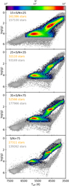 |
Fig. B.1 Same figure as Fig. 11 but for RVS stars parameterised by CNN only using RVS spectra. |
| In the text | |
 |
Fig. B.2 Same figure as Fig. 21 but comparing the CNN gravities (derived using only RVS spectra) and seismic gravities. |
| In the text | |
 |
Fig. C.1 Two-dimensional density distribution of the CNN minus APOGEE and calibrated GSP-Spec minus APOGEE as a function of Gaia DR3 radial velocity uncertainties in both the training (2 606 stars) and observed samples (20 948 stars, within the training sample limits). |
| In the text | |
Current usage metrics show cumulative count of Article Views (full-text article views including HTML views, PDF and ePub downloads, according to the available data) and Abstracts Views on Vision4Press platform.
Data correspond to usage on the plateform after 2015. The current usage metrics is available 48-96 hours after online publication and is updated daily on week days.
Initial download of the metrics may take a while.


