| Issue |
A&A
Volume 693, January 2025
|
|
|---|---|---|
| Article Number | A228 | |
| Number of page(s) | 28 | |
| Section | Galactic structure, stellar clusters and populations | |
| DOI | https://doi.org/10.1051/0004-6361/202452527 | |
| Published online | 21 January 2025 | |
CARMENES input catalogue of M dwarfs
IX. Multiplicity from close spectroscopic binaries to ultra-wide systems
1
Centro de Astrobiología, CSIC-INTA,
Camino Bajo del Castillo s/n, Campus European Space Astronomy Centre,
28692
Villanueva de la Cañada, Madrid,
Spain
2
Departamento de Física de la Tierra y Astrofísica & IPARCOS-UCM (Instituto de Física de Partículas y del Cosmos de la UCM), Facultad de Ciencias Físicas, Universidad Complutense de Madrid,
28040
Madrid,
Spain
3
UNIE Universidad, Departamento de Ciencia y Tecnología,
Arapiles 14,
28015
Madrid,
Spain
4
Instituto de Astrofísica de Andalucía (CSIC),
Glorieta de la Astronomía s/n,
18008
Granada,
Spain
5
Instituto de Astrofísica de Canarias,
Vía Láctea s/n,
38205
San Cristóbal de La Laguna,
Tenerife,
Spain
6
Departamento de Astrofísica, Universidad de La Laguna,
Astrofísico Francisco Sánchez s/n,
38206
La Laguna,
Tenerife,
Spain
7
Department of Astronomy and Astrophysics, University of California,
San Diego,
9500 Gilman Drive, La Jolla,
CA
92093,
USA
8
Landessternwarte, Zentrum für Astronomie der Universität Heidelberg,
Königstuhl 12,
69117
Heidelberg,
Germany
9
Institut für Astrophysik und Geophysik, Georg-August-Universität-Göttingen,
Friedrich-Hund-Platz 1,
37077
Göttingen,
Germany
10
Institut de Ciències de l’Espai (CSIC-IEEC),
Can Magrans s/n, Campus UAB,
08193
Bellaterra, Barcelona,
Spain
11
Institut d’Estudis Espacials de Catalunya (IEEC),
08034
Barcelona,
Spain
★ Corresponding author; This email address is being protected from spambots. You need JavaScript enabled to view it.
Received:
8
October
2024
Accepted:
28
November
2024
Abstract
Context. Multiplicity studies greatly benefit from focusing on M dwarfs because they are often paired in a variety of configurations with both stellar and substellar objects, including exoplanets.
Aims. We aim to address the observed multiplicity of M dwarfs by conducting a systematic analysis using the latest available astropho-tometric data.
Methods. For every star in a sample of 2214 M dwarfs from the CARMENES catalogue, we investigated the existence of resolved and unresolved physical companions in the literature and in all-sky surveys, especially in Gaia DR3 data products. We covered a very wide range of separations, from known spectroscopic binaries in tight arrangements (~0.01 au) to remarkably separated ultra-wide pairs (~105 au).
Results. We identified 835 M dwarfs in 720 multiple systems, predominantly binaries. Thus, we propose 327 new binary candidates based on Gaia data. If these candidates are finally confirmed, we expect the multiplicity fraction of M dwarfs to be 40.3−2.0+2.1%. When only considering the systems already identified, the multiplicity fraction is reduced to 27.8−1.8+1.9%. This result is in line with most of the values published in the literature. We also identified M-dwarf multiple systems with FGK, white dwarf, ultra-cool dwarf, and exoplanet companions, as well as those in young stellar kinematic groups. We studied their physical separations, orbital periods, binding energies, and mass ratios.
Conclusions. We argue that based on reliable astrometric data and spectroscopic investigations from the literature (even when considering detection biases), the multiplicity fraction of M dwarfs could still be significantly underestimated. This calls for further high-resolution follow-up studies to validate these findings.
Key words: astronomical databases: miscellaneous / virtual observatory tools / binaries: general / stars: late-type
© The Authors 2025
 Open Access article, published by EDP Sciences, under the terms of the Creative Commons Attribution License (https://creativecommons.org/licenses/by/4.0), which permits unrestricted use, distribution, and reproduction in any medium, provided the original work is properly cited.
This article is published in open access under the Subscribe to Open model. This email address is being protected from spambots. You need JavaScript enabled to view it. to support open access publication.
1 Introduction
Stellar multiplicity is a natural consequence of the stellar formation process (Chabrier 2003; Goodwin et al. 2007; Bate 2012; Tokovinin 2018, also see Duchêne & Kraus 2013 and Offner et al. 2023 for reviews). The frequency of multiple systems is known to increase with the primary stellar mass (Lada 2006; Parker & Meyer 2014; Offner et al. 2023). The observational evidence shows that multiplicity is greater than 80% for OBA-type stars (Kouwenhoven et al. 2007; Mason et al. 2009; Chini et al. 2012), around 50% for solar-type stars (Abt & Levy 1976; Duquennoy & Mayor 1991; Raghavan et al. 2010), and 10–30% for very low- mass stars and brown dwarfs (Burgasser et al. 2003, 2007; Bouy et al. 2003; Joergens 2008; Fontanive et al. 2018). In the case of M dwarfs, several studies in the last three decades have pointed to a multiplicity of 20–30% (e.g. Janson et al. 2012; Ward-Duong et al. 2015; Cortés-Contreras et al. 2017; Winters et al. 2019a; Clark et al. 2024).
If all stars are indeed born together with their siblings in groups, it is natural to question how single stars came to be. Many of them may not have remained together as they evolved, while a significant fraction could also remain undetected.
The dynamical interplay between the components turns into a competition for attaining stable orbits (Elliott et al. 2014; Sadavoy & Stahler 2017, but see King et al. 2012). It comes as no surprise that young stars are usually found to be part of multiple systems (e.g. Leinert et al. 1993; Reipurth & Zinnecker 1993; Kouwenhoven et al. 2007; Shan et al. 2017). The lifetimes of young systems are too short for them to have settled down into stable configurations (we refer e.g. to the simulations carried out by Allison & Goodwin 2011). For them, it is often unclear whether a given group of stars can be treated as a young trapezia-like architecture, a small stellar kinematic group, or a mature mini-cluster (Mamajek et al. 2010; Tokovinin 2022; González-Payo et al. 2023).
Systems that contain more than two components are, in principle, unstable (Harrington 1972; Goodwin & Kroupa 2005). However, the dynamical evolution is able to produce a hierarchical arrangement of binaries within binaries or nested orbits, which leads to stability (Evans 1968; Bonnell et al. 2003; Tokovinin 2014; Powell et al. 2023). In their seminal work, Poveda et al. (1967) numerically simulated the formation of runaway stars in few-body clusters, where the high kinetic energy of the runaways is balanced by the binding energy of the binaries formed during close interactions. The loss of angular momentum during the shrinkage of the closest pair is transferred to the third component, which can result in an ejection from the original compact arrangement, a process that unfolds during the first tens to hundreds of millions of years1 (Delgado-Donate et al. 2003; Tokovinin et al. 2006; Moeckel & Bate 2010; Kouwenhoven et al. 2010, and especially Reipurth & Mikkola 2012). A consequence of the momentum transfer is that a large fraction of close binaries are part of hierarchical triple systems (e.g. Czavalinga et al. 2023), a fact that different investigations noted some time ago (e.g. Mazeh 1990; Bate et al. 2003; Tokovinin et al. 2006; Pribulla & Rucinski 2006; Basri & Reiners 2006; Caballero 2007; Kouwenhoven et al. 2010; Rappaport et al. 2013, and see some examples by Cifuentes et al. 2021). This means that in many instances of wide binaries, one of the components is (or will be) further resolved as a very compact binary itself. The Proxima–α Cen AB triple system constitutes the nearest example of this kind. Luckily, from a mathematical perspective, these configurations can be treated dynamically as two-body problems (e.g. Evans 1968). However, the formation of close binaries in triple systems has also been linked to the Kozai–Lidov mechanism (Kozai 1962; Lidov 1962), but this has been challenged by the discovery of many wide tertiaries with isotropic orientations and low eccentricities that are inconsistent with the mechanism’s predictions (Hwang 2023).
While an upper limit for binary separation is not formally established, wide binary systems, particularly those exceeding 0.1–0.2 pc, are extremely fragile and can be easily disrupted by the Galactic field (Weinberg et al. 1987; Caballero 2009; Tokovinin 2017; González-Payo et al. 2023). Increasingly refined data from surveys such as Hipparcos (Perryman et al. 1997), Tycho-2 (Høg et al. 2000), and its successor Gaia (Gaia Collaboration 2016) have shown that stellar systems with very large orbital separations (of up to 1 pc or greater) do exist (Caballero 2010; Shaya & Olling 2011; Oh et al. 2017; Andrews et al. 2017). The conclusion of these analyses is that there is no strict cut-off in the semimajor axis (a) of wide binary systems, as previously theoretically predicted by Wasserman & Weinberg (1987); rather, a cut-off in binding energy is more likely (min  ; Caballero 2010). Proxima Centauri serves as an example of a star that remains bound to its system despite having a value of a roughly similar to the Hill radius of α Centauri AB (Matthews & Gilmore 1993; Wertheimer & Laughlin 2006; Reipurth & Mikkola 2012; Kervella et al. 2017).
Momentum transfer is not the only mechanism to account for the large separations of the widest binary systems. Considering two modes of binary breakup, namely, core splitting and stellar ejection, Sadavoy & Stahler (2017) predicted that the majority of wide binaries break apart, but with some systems becoming tighter within several million astronomical units (au). Goodwin & Kroupa (2005) noted that these ejections in hierarchical systems would also produce a significant population of close binaries that are typically only detectable using advanced techniques. Some binaries are so closely packed that they are disguised as single objects by direct imaging. While very close binaries are undetectable by direct imaging, they can be recognised in the Doppler shift of the spectral lines (spectroscopic binaries), in the periodic eclipsing of their light (eclipsing binaries), or in the measurable change in their motion (astrometric binaries). There are also compact unresolved triples with hierarchical orbits (Mazeh et al. 2001; Baroch et al. 2021, even existing within a space of only a few au; see Moharana et al. 2024). The lack of detailed observations regarding many individual stars carries an important observational bias, leaving some very close pairs unrecognised as such. Kroupa et al. (1991) found that previous studies had underestimated the number of low-mass stars and proposed that assuming independent component masses for binary systems reconciles discrepancies between different luminosity function samples. Piskunov & Mal’Kov (1991) noted that the impact of photometrically unresolved binaries on the luminosity function depends on the mass ratio, q = ℳ2 /ℳ1 , and is strongest when both components have similar masses.
Stars in multiple systems offer the precious opportunity to directly measure fundamental parameters, such as masses, radii, or both (e.g. Popper 1980; Mathieu et al. 2000; Zapatero Osorio et al. 2004; Torres et al. 2010; Schweitzer et al. 2019). However, close companions are capable of influencing every stage of the stellar evolution. Stars that have a common origin must have the same age and chemical composition. Therefore, wide binaries are assumed to be coeval (Hartigan et al. 1994; White & Ghez 2001; Jørgensen & Lindegren 2005; Stassun et al. 2006; Makarov et al. 2008; Kraus & Hillenbrand 2009), as well as cochemical (Gizis 1997; Gray et al. 2001; Desidera et al. 2004, 2006; Kraus & Hillenbrand 2009; Hawkins et al. 2020). Sufficiently resolved pairs can be useful to prove this assumption and serve as pieces in the puzzle of the Galactic formation. Fitting these pieces together and reassembling the original configuration is the goal of Galactic archaeology studies, which benefits from wide pair systems (Andrews et al. 2019; Hawkins et al. 2020). Important applications of wide binaries are the calibration of metallicities of M dwarfs (e.g. Bonfils et al. 2005; Bean et al. 2006; Lépine et al. 2007; Rojas-Ayala et al. 2010; Montes et al. 2018; Marfil et al. 2021), age-metallicity relation (e.g. Rebassa- Mansergas et al. 2016; Zhang et al. 2024), age–magnetic activity relation (e.g. Garcés et al. 2011; Chanamé & Ramírez 2012; Kiman et al. 2021), and even investigations into the dark matter in the Milky Way (e.g. Yoo et al. 2004; Chanamé & Gould 2004). The statistics regarding the frequency of multiple systems, their primary-companion mass ratios and their physical separations can also set meaningful constraints for models of stellar formation and evolution. For instance, they can help determine whether a primordial population composed exclusively of multiples is as likely as predicted (Hartigan et al. 1994; White & Ghez 2001; Parker et al. 2009; Reggiani & Meyer 2011; Clark et al. 2012; Leigh & Geller 2013; Reipurth et al. 2014; Parker & Meyer 2014).
Studies of stellar multiplicity take on particular significance for M dwarfs because they potentially rely on a vast sample of study. The nearest stars represent a valuable sample for multiplicity studies because they allow accurate photometric and astrometric measurements. Their multiplicity characteristics carry the imprints of the formation and evolution of our Galaxy. Although intrinsically small and faint (ℳ ≲ 0.62 M⊙, 𝓛 ≲ 0.076 L⊙ , Cifuentes et al. 2020, and references therein), M dwarfs make up the majority of the stars in the Galaxy (Henry et al. 1994, 2006; Reid et al. 2004; Bochanski et al. 2010; Winters et al. 2015; Reylé et al. 2021; Golovin et al. 2023; Kirkpatrick et al. 2024). M dwarfs have also gained importance in the last two decades because of the search for Earth-like planets, especially in their habitable zone (Scalo et al. 2007; Kopparapu et al. 2013), either with space missions for transit surveys (CoRoT, Auvergne et al. 2009, Kepler, Borucki et al. 2010, TESS, Ricker et al. 2014) or with the radial-velocity (RV) method (Bonfils et al. 2013; Fouqué et al. 2018; Reiners et al. 2018; Ribas et al. 2023). Among the notable high-resolution ground-based spectrographs that undertake RV searches is the Calar Alto high-Resolution search for M dwarfs with Exoearths with Near-infrared and optical Échelle Spectrographs2 (CARMENES, Quirrenbach et al. 2014).
Table 1 displays the multiplicity fraction (MF) of M dwarfs, namely, the proportion of these stars that are the most massive components of a multiple system (Sect. 4.1), along with the values reported in the literature by different authors during the past three decades, including the present work. We indicate (when possible) the relevant constrains of the studies: spectral range, sample size, completeness volume, search separations, and methodology. Not all the portions of the spectral range of M dwarfs have been studied equally well regarding their multiplicity. Also, the detection limits (again Sect. 4.1) are not consistent between studies, leading to different proportions of undetected binaries in very compact arrangements. While it has not been included in the list due to greater difficulty in comparison, we mention other systematic efforts in multiplicity investigations, such as the pioneering infrared imaging of 55 low-mass binaries by Skrutskie et al. (1989) or the Hubble Space Telescope snapshot high-resolution images of 225 stars by Dieterich et al. (2012). Many of the publications in Table 1 predate Gaia, but some of them made predictions on Gaia’s impact on M-dwarf multiplicity. For instance, Winters et al. (2019a) foresaw that Gaia’s astrometric measurements over five years would enable the detection of low-mass binaries that remained undetected, providing a more complete picture of the nearby M dwarf population.
This is the ninth paper of the series of publications on the CARMENES input catalogue of M dwarfs. CARMENES aims to look for Earth-like planets around the closest, brightest, late-type stars with the radial velocities technique. In this work, we present an updated and systematic study of the multiplicity across all spatial separations in the brightness-spectral type-limited CARMENES input catalogue. The sample under study is a collection of more than two thousand M dwarfs as described in Sect. 2. Our study exploits the fruitful Gaia mission (up to the third data release, DR3, Gaia Collaboration 2023b) to provide an updated revision of the multiplicity of M dwarfs, accounting for the impact of unresolved binaries on the MF. Since many definitions in this investigation are based on the resolution of the system components by the Gaia mission, in our analysis (in Sect. 3) we distinguish between systems with resolved and unresolved components in DR3. Section 4 is centred on results and discussion, which includes the description of the identified systems and their fundamental parameters. In particular, we differentiate between the canonical MF (Sect. 4.1) and the expected multiplicity fraction, MF+, which accounts for potential unresolved systems that could boost MF by more than 10%. The conclusions are summarised in Sect. 5. Finally, the appendix compiles and organises useful data produced in this work. Table 2 offers twelve tables with a variety of content. In particular, Table A.1 includes an abridged version of the full dataset compiled and produced in this work.
Multiplicity fraction for M dwarfs calculated in this work and published in the literature.
Summary of the tables appended to this work.
2 Sample
The CARMENES project selected 350 M dwarfs as the targets for the main survey, whereby a total of 750 useful nights were reserved as guaranteed time observations, from 1 January 2016 to 31 December 2020. The observations of the guaranteed time observations sample continue within the CARMENES Legacy+ programme, which aims for 50 measurements for all suitable targets and is expected to run at least until the end of 2025. The raw data, calibrated spectra, and high-level data products were made publicly available as the CARMENES Data Release 1 (Ribas et al. 2023). The continuous update of the catalogue has introduced additional M dwarfs to the original sample, mostly objects of interest (TOI) identified by the Transiting Exoplanet Survey Satellite programme (TESS; Ricker et al. 2014). RV follow-up has confirmed many of these transiting exoplanets (e.g. González-Álvarez et al. 2023; Goffo et al. 2024; Kuzuhara et al. 2024; Dai et al. 2024, just to mention a few recent ones). The left panel of Fig. 1 illustrates the distribution of M dwarfs in our sample according to spectral subtype. The latest-type star is an M9.5 dwarf, Scholz’s star (Karmn3 J07200–087).
The full sample of our study is dubbed Carmencita, the input catalogue for the CARMENES project (Alonso-Floriano et al. 2015; Caballero et al. 2016). Carmencita contains a total of 2214 M dwarfs, from M0.0 V to M9.5 V, including the targets for the main survey. The stars were intentionally chosen independently of their multiplicity, age, or metallicity. Only one Carmencita object classified as K7 V (HD 97101) remains in the RV-monitored sample, as it is the bound companion of an M2 V star (HD 97101 B). All these stars satisfy simple selection criteria based on their spectral types, their visibility from the Calar Alto Observatory in Southern Spain (δ ≳ –23 deg), and on their apparent brightness in the J-band magnitude, between 4.2 mag and 11.5 mag (this range of magnitudes also depends on spectral type, as detailed by Alonso-Floriano et al. 2015). The stars in our sample are located at distances ranging between 1.82 pc (Barnard’s star) and 166.1 pc (Haro 6-36), with the majority of them in our immediate vicinity, with a median distance of 22.0 pc.
Magnitude-limited samples may be unintentionally overpopulated by intrinsically bright unresolved stellar systems due to the Malmquist bias (see Duquennoy & Mayor 1991, and references therein). In particular, these samples may over-represent spectroscopic binaries because two stars are brighter than one. Since Carmencita started to be built well ahead of the Gaia launch, it is not a volume-limited sample. Furthermore, by construction it is not a magnitude-limited sample (the faintest M0.0–0.5 V stars are several magnitudes brighter in J than the brightest late-type M dwarfs). Therefore, we calculated a ‘completeness distance’, dcom, that depends on the spectral type. We used the definition of absolute magnitude in the J band, MJ – J = 5 – 5 log dcom , where J = J(SpT) from the construction of Carmencita (Table 1 from Alonso-Floriano et al. 2015), and MJ = MJ (SpT) from an empirical relation (Table 7 in Cifuentes et al. 2020). Therefore, dcom(SpT) is the radius of the sphere that contains all known M dwarfs with an equal or earlier spectral type. As a result, Carmencita contains all M dwarfs with spectral types M4.5 V or earlier up to 30 pc, and all M dwarfs with spectral types M9.5 V or earlier up to 10 pc. The latter finding was double-checked against the 10 pc sample study by Reylé et al. (2021). The right panel of Fig. 1 aims to illustrate this fact. Of course, this completeness is contingent on the additional condition that the stars must be visible in the northern hemisphere.
3 Analysis
3.1 Search for resolved systems
A schematic summary of this analysis is displayed in Fig. 2. For each star in our M-dwarf sample, we started by searching for resolved physical companions in two steps. First, we reviewed the Washington Double Star catalogue4 (WDS; Mason et al. 2001), and then we performed a dedicated, blind search employing the most updated astrometric information available from Gaia (i.e. DR3). In this context, a resolved physical companion (of a given star) is defined as an individual source in an astrometric catalogue such as Gaia with proper motions and trigonometric parallax that are compatible with physical binding with the primary.
As a preliminary step, we got equatorial coordinates at the 2016.0 Gaia epoch and apparent magnitudes in G for 100% of our sample using the Gaia Archive5. Next, we ensured that each of our objects had a complete astrometric description. The full, five-parameter solution from Gaia DR3 (position, proper motion, and parallax: α, δ, µα cos δ, µδ, ϖ) is available for 93.0% of the 2214 M dwarfs. Among them, 61.2% also have barycentric radial velocity, Vr, from the second or third data releases of Gaia; we prefer the latter in case of availability in both. For the sources for which Gaia does not provide some of these data, we searched in the literature for published measurements (e.g. Gliese & Jahreiß 1991; van Leeuwen 2007; Faherty et al. 2012; Dittmann et al. 2014; Finch & Zacharias 2016). Of the remaining 4.9% of stars without full Gaia solution, we compiled proper motions and parallaxes from other sources for all except for 34 (see below).
We performed a cross-match of our Gaia stars with WDS utilising the Tool for OPerations on Catalogues And Tables (TOPCAT; Taylor 2005). The WDS is the principal database for astrometric double and multiple star information, collecting 156 861 systems to submission date. For many of them, it compiles precise astrometric history and orbital description, making it a valuable resource for our study. In the WDS catalogue we found 411 systems that contain at least one M dwarf from our sample. For them, we retrieved the last measured epoch (sep2), the corresponding position angle (pa2), and separation in the ‘precise’ format (i.e. non-rounded values), and incorporated them in the final table. We took into account that our M dwarfs could be either the WDS primary or a companion. At this stage we added one star and eight T-type dwarfs in multiple systems that are not tabulated by Gaia because of their brightness (Capella) or their faintness (e.g. GJ 570D, Ross 458C), respectively.
After identifying the resolved pairs already documented by WDS, we also looked for common proper motion and parallax companions within the Gaia data. We performed a blind search using the DR3 by dividing the search in two ranges of separations. First, for the closest systems, we used the automatic positional cross-match tool in TOPCAT, X-match, limiting to a search radius of 5 arcsec and setting the ‘find’ option to ‘all’. With this configuration we made sure to keep every source found in the vicinity of our sources, regardless of its apparent magnitude, parallax distance, or proper motion, even when some of this information was not available. Second, we conducted a much wider, separation-limited search using the Astronomical Data Query Language (ADQL) form in the Gaia Archive. We limited the search to a physical separation of 105 au (∼0.5 pc), which translates to projected separations of 20 000–2000 arcsec for stars located at distances of 5–50 pc. As mentioned in Sect. 1, there is no consensus regarding an upper limit in wide binary separation. Therefore, we set a safe upper limit of 105 au to ensure that actual bound systems with remarkable separations were not missed in the process, but keeping in mind that projected separations are always less than or equal to the true separations (see e.g. Wertheimer & Laughlin 2006). In this search we looked for resolved sources with full five-parameter astrometric solutions compatible with physical binding to our source. To begin with, we automatically kept all the sources with separations ρ > 5 arcsec exhibiting a conservative difference in their parallactic distances of 10% with respect to our star, namely, distance ratio:
 (1)
(1)
For these sources, we computed two additional metrics to ensure that they are approximately co-moving. These are the µ ratio and the proper motion position angle difference, ∆PA, defined by Montes et al. (2018) and used afterwards by Cifuentes et al. (2021) and González-Payo et al. (2023):
 (2)
(2)
 (3)
(3)
This search recovered all 568 pairs known in WDS that Gaia is able to resolve (Sect. 4.3.1). In Fig. 3, we compare the values of angular separations tabulated by the WDS with those computed by us using the Gaia astrometry. There are only 15 pairs of stars (shown in magenta) with separation differences larger than 10% between WDS and our measurements. They correspond to well-documented binaries with very small projected separations (ρ ≲ 2 arcsec) that exhibit significant orbital motion over relatively short timescales (of a few years; e.g. BL Cet + UV Cet, Wolf 424 AB, or AT Mic AB – the three of them located at less than 10 pc from the Sun). The observed scatter of the 1:1 relation justify a posteriori our 10% distance ratio criterion. This scatter is due to a mixture of systematic effects on parallax, such as colour-dependent effects, under-estimated uncertainties of faint sources, or impact of unresolved binarity.
Figure 4 shows a comparative analysis of the proper motions (∆PA vs µ ratio; top panel) and distances (companion’s d vs primary’s d; bottom panel) of the identified pairs. The majority of our pairs comply with the criteria for physical association (shown in blue), although there are 78 sources (shown in red and amber) that exhibit anomalies in their relative positional angles, proper motions, or distances. Our individual examination of these sources allowed us to propose the most likely reasons for these outliers, and to keep all of them as very interesting instances of binarity, as summarised in Table A.2. Most of these outliers exhibit proper motion and parallax anomalies (Kervella et al. 2019; Brandt 2021) due to the closeness of the components. Their orbital periods are for this reason relatively short, of a few tens of years or less (Sect. 4.3.3). The systems containing some of these pairs are valuable because their dynamical masses could be determined in the near future.
In addition, there are 34 systems in which distances and proper motions are missing for one of the components, and so ∆d, µ ratio, and ∆PA are unknown. For these, our criteria for physical associations are not fully conclusive, but they do all correspond to well-characterised close binaries listed by WDS, which we retained in our analysis nevertheless.
Even though for most of the cases, the criteria presented here are effective for determining whether a pair of components in a system is physical or optical (unbound), there are some caveats. False positives (or chance alignments) can be found in wide pairs (Sect. 4.3.1 offers a deeper analysis), while false negatives, attributed to imprecise astrometry, are more commonly found in very close pairs. The nominal operations of Gaia up to DR3, spanning 1028 days, may not provide sufficient coverage, leading to ill-defined proper motions in those cases for which orbital periods notably exceed this timespan. Thus, these may reflect the instantaneous tangential path, including orbital motion, meaning that some bound systems might not qualify as binary. Given the small probability of finding a source at a similar distance within a small search radius, the benefit of finding a close companion justifies the effort of checking individually all the potential pairs by accessing to images and catalogues. For this particular inspection we used the Aladin interactive sky atlas (Bonnarel et al. 2000) and the SIMBAD database (Wenger et al. 2000). With Aladin we carefully examined every source at a separation ρ < 5 arcsec from our targets, discarding those with an astrometric description that identified them as background objects.
Most of the systems discovered in our Gaia blind search are tabulated by the WDS, as illustrated by Fig. 3. From a total of 720 systems found in our sample, 697 are tabulated in the WDS, of which 249 are not resolved by Gaia. Many of them are very close sub-arcsecond binaries detected with adaptive optics, lucky imaging, or speckle interferometry (Sect. 4.3.1), but there is also room for resolved ultra-cool dwarfs that are fainter than the Gaia magnitude limit (Sect. 4.4.3).
Despite the continued efforts by the WDS team at the United States Naval Observatory to keep this catalogue updated, there can still be missing pairs that appear in the literature. To address this gap, we also cross-matched our stars with the Robo-AO surveys (with d ≲ 30 pc) of Lamman et al. (2020) and Salama et al. (2022), the Gaia catalogue of nearby stars (GCNS, Gaia Collaboration 2021b), the million binaries from Gaia EDR3 of El-Badry et al. (2021), the 10-parsec sample of Reylé et al. (2021), the full-sky 20-pc census of Kirkpatrick et al. (2024), and the ultra-cool dwarf companion catalogue by Baig et al. (2024). Some of these compilations (mostly El-Badry et al. 2021 and Gaia Collaboration 2021b) tabulated bound systems that are not yet tabulated in the WDS, but were also identified by us. For completeness, we also cross-matched the remaining systems with the Washington Double Star Supplemental Catalog6, which besides compiles the input from those and other large faint duplicity surveys such as those by Dhital et al. (2015), Oh et al. (2017), Tian et al. (2020), or Hartman & Lépine (2020). Their findings are duly credited in the ‘Discoverer’ column across the various tables in this work.
While most pairs found in our custom Gaia search are known, either from WDS or the recent searches mentioned before, we report six physically bound systems for the first time. All but two are considered to be single stars; the exceptions are the triple systems HD 230017 in the Carina moving group (Sect. 4.5) and GJ 3261, which were thought to be close binaries. We show the six new systems in Table A.3. Apart from Gaia DR3 astrometric solutions (α, δ, ϖ, µtotal), for each pair, we tabulated their angular separations (ρ) and position angles (θ).
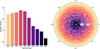 |
Fig. 1 Distribution of spectral types of the stars in the sample (left) and illustration of the completeness distance of Carmencita (right). The latter panel shows the distance and right ascension α of the Carmencita stars in the solar neighbourhood and colour-codes the spectral subtype as a function of the distance to which our sample is complete. The dashed lines depict 10-parsec increments of the distances. |
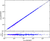 |
Fig. 3 Comparison of projected separations tabulated by the WDS and measured by us using Gaia astrometry. The solid and dashed grey lines represent the 1:1 relation, and the differences in 10%, respectively. The magenta circles are stars beyond this limit. The error bars are rather small for almost all cases due to the high precision of Gaia’s astrometry and they have therefore been omitted. |
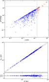 |
Fig. 4 Comparative analysis of the proper motions and distances of the identified pairs. Top: ∆PA vs µ ratio diagram, where the dashed grey lines set the upper limits of our criteria for physical association (Eqs. (2) and (3)). The red open circles are pairs that do not comply, or do so partially, with those criteria, respectively. Bottom: comparison of distances of the companions (denoted ‘B+’) and their corresponding primaries (‘A’). The amber circles are pairs that do not comply with our criterion (Eq. (1)). Our Carmencita M dwarf may be the primary (i.e. the most massive) or a companion in the system. |
3.2 Search for known spectroscopic binaries
After determining the systems in our sample that are astro- photometrically resolved by Gaia, and those tabulated by WDS and other recent catalogues, we carefully reviewed the literature for references to unresolved systems, namely spectroscopic binaries 7 (SBs). For a comprehensive list of SBs, the main source of reference used in this work was the 9th Catalogue of Spectroscopic Binary Orbits (SB9, Pourbaix et al. 2004). In this catalogue, we found 166 spectroscopic multiples among the stars in our sample and their companions for which a spectroscopic investigation has been conducted (we refer to Sect. 4.1 for an explanation of the detection limits of the Carmencita stars and their physical companions). Among them, we found 42 cases in which the components have also been astrometrically resolved and compiled in the WDS. By checking the reported orbital periods and magnitude differences we ensured that both measurements refer in fact to the same pair. For these cases we removed the spectroscopic binary designation (Aab) and classified them as close resolved, AB or (AB). In case of doubt, we preferred to stay conservative and avoided losing a potential triple system (thought to be simply double) in a compact configuration. For instance, the physical pair GJ 3481 and GJ 3482 (COU 91), where the latter is further resolved as a spectroscopic binary (a < 0.66 au according to Shkolnik et al. 2010) and as an astrometric visual pair with the FastCam lucky imager (ρ ≈ 0.94 arcsec or s ~ 16.7 au according to Cortés-Contreras et al. 2017), might potentially constitute a hierarchical quadruple. Another example is GJ 3522 (LHS 6158), a 7.6-day doublelined spectroscopic binary (Reid & Gizis 1997; Tokovinin 2018), with a third component in a 5.7-year period (Hartkopf et al. 2012) revealed using adaptive optics (Delfosse et al. 1999), with spectral classification assumed roughly similar to the primary’s (M3.5 V, Kirkpatrick et al. 2012) and constituting one of the nearest (d = 6.7 pc) hierarchical triples. A total of 124 spectroscopic systems found in our sample and are listed in Table A.4, including their published orbital periods, Porb, semimajor axes, a, and mass ratios, q = ℳB/ℳA, together with their references. Values estimated from mass–luminosity relations, or directly from spectral typing, are not collected. None of the 123 SBs have been spatially resolved to date.
The cases in which the orbital plane of a binary system aligns with our line of sight are rare. Eclipsing binaries (EBs) are a unique category and serve as a valuable opportunity for determining empirical masses and radii (Huang & Struve 1956; Popper 1980; Andersen 1991). EBs enable the measurement of dynamical masses, especially in detached double-lined SBs, and provide accurate radius measurements with precision around 1– 2% (Ribas 2003; Torres et al. 2010; Schweitzer et al. 2019). These parameters have the advantage of not relying on models, so they can serve to evaluate the accuracy of theoretical predictions. Shan et al. (2015) demonstrated an elevated occurrence of eclipsing binaries among detached M-dwarf SBs with orbital periods of 1–90 d, exceeding previous RV-based inferences. Stellar activity levels, particularly in young, magnetically active, or fast-rotating tidally-locked eclipsing binaries, can also introduce biases, leading to observed inflated radii (Caballero et al. 2010; Jackson et al. 2018; Kesseli et al. 2018; Parsons et al. 2018). Allsky surveys such as Kepler and TESS have made possible the identification of eclipsing binaries by the thousands (Kirk et al. 2016; Prša et al. 2022). In our sample there are five known eclipsing binaries, which are listed along with their masses and radii in Table A.5. Additionally, the objects GJ 3547 (J09193+620), GJ 3461 (J07418+050), and GJ 3793 (J13348+201) are suggestive of eclipsing events from the study of TESS light curves (Skrzypinski 2021). The first two are double-lined spectroscopic binaries (in one case also featured in the variability catalogue of Eyer et al. 2023), while the third is a single star but flagged by us as a likely unresolved binary (‘candidate’; see Sect. 3.3).
3.3 Search for new binary candidates using Gaia
Next, we exploited the wealth of Gaia data in order to identify binary candidates that have not been identified in previous work. This analysis also extended to companions of known multiple systems found in the previous sections, which added complexity to a number of these systems.
The spatial resolution of Gaia was limited to 0.4–0.5 arcsec in the second data release (DR2, Gaia Collaboration 2018), and slightly improved in the early third data release (EDR3, Gaia Collaboration 2021a). In particular, Fabricius et al. (2021) showed that EDR3 achieves completeness for separations larger than 1.5–2.0 arcsec, with a severe incompleteness below 0.7 arcsec. Objects closer than this limit can be identified with Gaia, but this identification depends on the magnitude difference, current angular separation, and orientation along the dominating scan directions (e.g. Gaia Collaboration 2021b). Gaia EDR3 data can be affected by spurious signals linked to the time-dependent scan angle of the instrument, leading to false periodic signals in photometry and astrometry. Using numerical simulations, Holl et al. (2023) explored how these biases occur and provided statistics to identify and filter affected sources. They found that these signals often originate from unresolved binaries or other close optical pairs with fixed orientations and separations of less than 0.5 arcsec (including binaries with orbital periods of several years). Therefore, Gaia EDR3 is capable of resolving visual double stars, but unable to resolve the closest pairs, with ρ ≲ 0.13 arcsec, although upcoming releases are expected to enhance these resolution capabilities (de Bruijne et al. 2015). Still, Gaia has been proven highly valuable to date in the detection of binary stars (see El-Badry 2024).
The third data release, DR3, maintains the same astrometric data as EDR3, but it includes a rich set of new data products that we exploited in this work. For instance, Gaia DR3 is the first release that provides an analysis of the RV time-series. By the time of this release, every source was observed with the Radial Velocity Spectrometer an average of ~70 times, varying from ~30 to ~240, depending on the sky coordinates.
Gaia DR3 comes with numerous statistical parameters to assess the reliability of the astrometric data. We summarise in Table 3 some of these quality indicators or combinations of them, which serve to flag stars with astrometric issues. They have been proven to be sensitive to the presence of potential unresolved companions (e.g. Fabricius et al. 2021; Katz et al. 2023; Pourbaix et al. 2022; Penoyre et al. 2022a; Shahaf et al. 2023; Van der Swaelmen et al. 2025). A detailed description of them can be found in the Gaia DR3 documentation8. The usage of these parameters is explained next (Sects. 3.3.1–3.3.4), as well as complementary methods of assessing unresolved multiplicity exploiting the Gaia products, which overlap with the criteria of Table 3 (Sects. 3.3.5–3.3.6). Figures 5 and 6 illustrate the different unresolved multiplicity criteria.
3.3.1 RUWE (Criteria 1 and 2)
Perhaps the most widely used metric in Table 3 is the renormalised unit weight error (RUWE), which evaluates the behaviour of the centre of light. Belokurov et al. (2020) showed that the amplitude of the centroid perturbation correlates with the physical separation between companions and scales with the binary period and mass ratio. Unresolved binaries with periods similar to or longer than the Gaia timespan (which increases with each subsequent release) can show elevated RUWE due to orbital motion affecting the astrometric fit (see Penoyre et al. 2022a for a detailed discussion). Castro-Ginard et al. (2024) suggested that the majority of binary systems in our Galaxy will remain undetected because the wobble of the centre of mass around the photocentre is largely masked by the astrometric noise from Gaia, leading to a RUWE value below the detection threshold (we refer to their Fig. 1 for an illustration). However, the median distance of our M-dwarf stars is 22.0 pc, which locates them in our immediate vicinity and allows to detect that wobble in many cases. Penoyre et al. (2020) noted that assuming an object as a single point mass in astrometry can bias measurements due to unresolved binaries. They also concluded that orbital motion with period near one year can mimic parallax, distorting distance estimates. Additionally, distant objects (further than 100 pc) can show disproportionate values of RUWE (Baig et al. 2024), which has been mitigated by an additional renormalisation, namely local unit weight error (LUWE, Penoyre et al. 2022b), with well- behaved single stars having a value close to 1.0. Still, RUWE remains a powerful and simple metric, especially when complemented with other indicators. Instead of the generally adopted value of 1.4 (e.g. Arenou et al. 2018; Lingam & Loeb 2018; Cifuentes et al. 2020), or even the position-dependent range of values from 1.15 to 1.37 developed by Castro-Ginard et al. (2024, their Fig. 3), in our analysis we set a conservative minimum of RUWE > 2.0, which leaves behind ∼80% of the sample.
Criteria for the detection of unresolved sources based on Gaia DR3 statistical indicators.
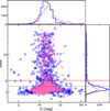 |
Fig. 5 RUWE as a function of G magnitude for single stars (pink open circles) and stars in multiple systems (open blue circles). The histograms follow the same colour coding. RUWE = 2.0 (thick red dashed line), used in this work, leaves behind ∼80% of the sample and is more conservative than the traditionally used RUWE = 1.4 (thin black dashed line). |
3.3.2 ipd metrics (Criteria 2 and 3)
The broad applications of many of the ipd metrics in the targeting of binary stars has been recognised, for instance, by Vrijmoet et al. (2020), who applied them to two decades of astrometric data from the RECONS program along with Gaia DR2 observations. Clark et al. (2022) demonstrated that Gaia was unable to resolve a great portion (58.9%) of the close companions that they detected using speckle imaging, which motivates the need for additional high-resolution imaging (∼40 mas). They investigated the usefulness of the metrics RUWE along with the parameter ipd_frac_multi_peak for assessing the likelihood of an unseen stellar companion (IPD stands for ‘image parameter determination’). For instance, Baig et al. (2024) built the ultra-cool dwarf companion catalogue exploring the likelihood of hidden binarity using LUWE and IPD.
Likewise, Golovin et al. (2023) identified sources with spurious astrometric solutions in their Fifth Catalogue of Nearby Stars (CNS5) by applying a simple cut on the ipd_gof_harmonic_amplitude (see their Eq. (2)). We did not include this criterion among ours, but we nevertheless applied it to every star and companion in our sample for which a measure of the parallax is available from Gaia DR3 (but excluding DR2). We found that only nine objects show spurious solution using this cut, with eight of them being known binaries, and one being single, but categorised as ‘Candidate’ via several other criteria in Table 3.
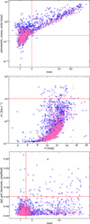 |
Fig. 6 Gaia DR3 statistical indicators of very close multiplicity. Top : astrometric_excess_noise (ϵ) vs RUWE. Middle : σ(Vr) vs G. Bottom: ipd_gof_harmonic_amplitude vs RUWE. In all panels, pink and blue open circles are for stars that were considered single and part of multiple systems, respectively, and the red thick dashed lines indicate the corresponding close binary selection criterion in Table 3. |
3.3.3 Variability in RV (Criteria 4 and 5)
The standard deviation of RV at several epochs (i.e. σ(Vr) = e_RV) is a powerful method of identifying (spectroscopic) binary systems. Furthermore, it allows to discriminate true orbital acceleration due to multiplicity from the acceleration due to an effect of perspective.
Among the stars with the largest σ(Vr) measured in Gaia DR3, greater than 10 km s−1, we selected the brightest ones to study their close multiplicity using medium-resolution spectra. We are carrying several observation campaigns with the high- resolution FIbre-fed Echelle Spectrograph (FIES) mounted on the 2.56 m Nordic Optical Telescope (NOT), in the mediumresolution mode (R = 46000), as well as with the High- Efficiency and high-Resolution Mercator Échelle Spectrograph (HERMES) at the 1.2 m Mercator telescope. From this ongoing program, we confirm the multiple nature of several of these candidates. Although the detailed results will be published in a forthcoming article, the preliminary results from those observations confirmed that our limit of 10 km s−1 is very robust.
3.3.4 Lacking or poor data (Criteria 6 and 7)
Sources in DR3 apparently unaffected by the proximity of other objects, but showing excessive uncertainties in parallaxes and proper motions nonetheless, or lacking entries in these fields altogether, could actually be close binary candidates. For example, Gaia Collaboration (2021b) noted that spurious astrometric solutions can be due, among a number of reasons, to the presence of more than one object in the astrometric window (close double systems, either real or in projection) or to binary orbital motion that is not accounted for. The odds for a chance alignment are much lower than for a physical connection, although these odds increase at wider separations and fainter magnitudes (e.g. El-Badry et al. 2021; Chulkov & Malkov 2022). Chance alignments are more likely to occur in regions of high surface density of sources such as open clusters and near the galactic plane (Gaia Collaboration 2021b). While DR3 benefits from a larger number of observation epochs with respect to previous releases, some very close binaries not resolved in DR2 were handled as single objects, with blended photometry and occasional spurious astrometric solutions (Arenou et al. 2018; Ziegler et al. 2018). The duplicated_source flag is usually of help for those sources that also exhibit poor astrometric quality or lack some data (mainly proper motions and parallaxes). This flag is set to ‘1’ in those instances where the detection system on board Gaia generates multiple detections for the same source, which results in different data sets for the same target. The final DR3 catalogue retained only the solution with the best astrometric quality and flagged it as a duplicated_source, while the poorer ones were discarded.
 |
Fig. 7 Light curves corresponding to the Gaia passbands GRP (red), G (green), and GBP (blue) for three cases: a single star (left), a known close (ρ = 0.1–0.2 arcsec) binary system (JNN 266, Janson et al. 2014b; middle), and a newly reported close (ρ ≈ 0.48 arcsec) binary system (right). Isolated outliers (represented by crosses) are photometric errors, not consistent with flares, automatically rejected by variability processing. The remaining light curves for the unresolved binary candidates with double-sequence patterns are displayed in Fig. A.1. |
3.3.5 Non-single star tables by Gaia DPAC
Among the built-in data products in Gaia DR3 by the Data Processing and Analysis Consortium (DPAC), the ‘non-single stars’ tables (Pourbaix et al. 2022) enable the identification of unresolved astrometric, spectroscopic, and eclipsing binaries (Gaia Collaboration 2023a). Despite their name, these tables are unrelated to the non_single_star flag, which is primarily a modelling quality flag and not an identifier of multiplicity. These solutions are distributed in four tables: nss_two_body_orbit when the full orbital motion is known, nss_acceleration_astro and nss_non_linear_spectro when a trend is known, and nss_vim_fl for photometrically variable unresolved binaries. More details on the processing scheme, its validation, and the various types of reached solutions can be found in Chapter 7 of the Gaia DR3 documentation.
3.3.6 Astrometric excess noise
In addition to RUWE, another measure of Gaia’s astrometric goodness-of-fit is the astrometric_excess_noise (ϵ). It quantifies the disagreement between the observations of a source and the best-fitting standard astrometric model. Both are sensitive to the photocentric motions of unresolved objects, such as astrometric binaries, which are not revealed by the IPD statistics, and therefore complement the latter in binary detection (Lindegren et al. 2021). For well-behaved sources, ϵ should be zero, but since it accommodates excess noise originating from both the source and the instrument attitude, non-zero values are inevitable (Lindegren et al. 2012). For instance, in DR1 nearly all sources show significant excess noise (ϵ ∼ 0.5 mas), but only unusually large values (ϵ ≳ 1–2 mas) are indicative of astrometric binarity or other issues (Lindegren et al. 2016). In DR2 roughly 20% of the sources between G = 12 mag and 20 mag have excess noise (Lindegren et al. 2018). In EDR3, Lindegren et al. (2021) observed an improved homogeneity of ϵ despite increased noise in crowded regions. Nevertheless, ϵ can be regarded as insignificant (i.e. effectively zero) if the significance, astrometric_excess_noise_sig (D), is less than 2 mas.
The RUWE includes a scaling factor to compensate for calibration errors that correlate with colour and magnitude, but ϵ does not. For example, Gandhi et al. (2022) used astrometric excess noise to search for candidate X-ray binaries, selecting sources with ϵ ≥ 0.01 mas, D ≥ 2 mas, visibility_periods_used > 10, and G between 13 mag and 20 mag. They found that systematic effects, such as attitude errors, partially resolved double stars, and source variability, can be sources of contamination, especially when ϵ < 1 mas, making interpretation more difficult.
In the stars of our sample, we found a linear correlation between the excess ϵ and its significance D, meaning that larger values of ϵ are generally associated to larger values of D. In particular, all the instances with notable ϵ happen to be known binaries in close configurations. Therefore, we found ϵ and D to be redundant and equivalent to RUWE, and stuck to the latter, as detailed in Sect. 3.3.1.
3.3.7 Photometric variability
Measuring the stellar brightness over time can reveal the presence of binaries that are otherwise indistinguishable in static images. Gaia DR3 provides a variability analysis of many objects using data from the 34 months. The variability processing and analysis was based mostly on time series of field-of-view transit (integrated) photometry in the calibrated G, GBP , and GRP bands, with additional input data, such as RV time series. We refer to Eyer et al. (2017) for a more complete description of the models and methods. In Gaia DR3, phot_variable_flag tags with ‘VARIABLE’ those sources identified and processed as variable from the photometric data. The variables GrVFlag, BPrVFlag, and RPrVFlag accompanying the photometric measurements indicate the photometry rejected by variability processing (Eyer et al. 2023). Even so, 346 stars in our sample are identified as variables by Gaia DR3.
Figure 7 shows the photometric time series (or light curves) in the three Gaia passbands for three selected cases: a single star, a known binary, and a binary candidate. When an object crosses the focal plane of Gaia (see Fig. 4 of Gaia Collaboration 2016), its flux is measured nearly simultaneously in the three passbands, but the G-band photometry is more precise and has a better spatial resolution (Eyer et al. 2017, additionally, the object is typically detected by nine CCDs in the green photometer, which is larger than the red and the blue). Stellar variability of intrinsic nature (i.e. not due to the presence of a companion) is apparent in the three passbands simultaneously and with a common pattern. However, there are Gaia sources with relatively flat GBP and GRP light curves, but much scattered G light curves. Sometimes they even display a double G light curve separated by up to 0.7 mag; these sources are actually close binary systems unresolved in GBP and GRP but resolved or partially resolved, depending mostly on the scan angle, in G (Vinagre Maqueda 2023; Maíz Apellániz et al. 2023; González-Payo et al. 2024; T. Prusti, priv. comm.). In the three examples of Fig. 7, only the G light curves of the known binary (LP 15–315, JNN 266) and our new candidate binary (RX J0507.2+3731B, ρ ≈ 0.48 arcsec) display a “double-sequence” pattern.
Figure 8 compares the standard deviation, σ, between two Gaia passbands. It distinguishes between multiple systems and single stars, and among these, the ones that are new unresolved binary candidates. Except for a few intrinsically variable young stars, single stars systematically show low standard deviations in the three passbands. All the sources with significant deviations are either confirmed binaries or close binary candidates. All the known binaries and new unresolved binary candidates in the agglomeration in top left corner show the G double-sequence pattern that is not detected in the GBP (and GRP) light curves.
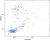 |
Fig. 8 Comparison of the standard deviations of GBP against that of G for single stars (light blue), stars in multiple systems (blue), and new unresolved binary candidates (red). The dashed line represent a 1:1 relation. The similar plot for GRP is omitted for simplicity. |
3.3.8 Selection of candidates
We used all the seven criteria of Table 3 to identify new candidate binaries among the M dwarfs of our sample and their Gaia companions (2634 stars, white dwarfs, and ultra-cool dwarfs in total). We found that 327 of them meet one or more of the criteria. Of them, 278 were thought to be singles and 49 formed part of multiple systems with known companions but are separated enough to exert a negligible influence. When the identified unresolved binary candidate is part of a known multiple system, we flagged them as ‘Multiple+’ in the full version of Table A.1.
If the candidate is a single star without known companions, we flagged them as ‘Candidate’.
Figures 5 and 6 illustrate the correlation of four selected statistics of Gaia: ipd_gof_harmonic_amplitude, ruwe, radial_velocity_error (criteria 1, 2, and 5 in Table 3), and astrometric_excess_noise. Stars in multiple systems may only have wide companions and, therefore, experience insignificant (if any) change in ruwe or  . Single stars are generally more scarce as we approach to the limits set by the criteria.
We also looked for matches of our sample (and their resolved companions) within non-single star tables provided by Gaia, and found 49, 6, 1, 0, and 2 coincidences in the tables enumerated in Sect. 3.3.5, respectively. These coincidences translate into 55 individual stars proposed as unresolved pairs by the Gaia processing scheme. Of them, 24 are known pairs with very closein orbits, and 31 are bona fide single stars, or in a few cases component in very wide pairs, presumably unaffected by their distant companion. The 2 eclipsing binaries are the known systems of Castor C (Joy & Sanford 1926; Gizis et al. 2002) and GJ 3547 (Shkolnik et al. 2010; Reiners et al. 2012). The former belongs to the sextuplet system α Gem, one of the most complex configurations in our sample.
Additionally, we matched our list of candidates with those identified in the GCNS by Penoyre et al. (2022b). This yielded 227 objects with both RUWE and LUWE values pointing to possible binarity. All of them are also tagged by us as candidates, except in those cases where close (or very close) multiplicity is already known. Additionally, we cross-matched the table vari_eclipsing_binary (Mowlavi et al. 2023; Eyer et al. 2023), which was the first Gaia catalogue of eclipsing binaries from the study of variability. No new EB candidates were found as a result.
4 Results and discussion
4.1 Multiplicity fraction
In the present work, we adopted the traditional definition for stellar multiplicity, requiring that the M dwarf is the primary (i.e. the most massive) component of its system. This means that M dwarfs as companions to A-type stars9, FGK stars (Sect. 4.4.1) and white dwarfs (Sect. 4.4.2) do not count towards multiplicity statistics. In order to quantify the observed multiplicity frequency or multiplicity fraction (MF) of M dwarfs, we followed the convenient notation of Batten (1973), who denoted as fn the fraction of primaries that have n companions:
 (4)
(4)
where S , B, T, Q represent the number of single, binary, triple, and quadruple systems, respectively. In our sample of 2214 M dwarfs, 834 (37.7%) belong to a multiple system, and from these almost three out of four (73.8% or 615) are the primaries of their systems, which implies a multiplicity fraction of  , where the uncertainties correspond to the 95% confidence interval using the Wilson formula (Wilson 1927). The remaining 1377 (62.2% of the total) stars did not have suspected companions at any separation until now, with the exception of exoplanet hosts (Table A.11). However, 278 of them (plus 49 wide components among those in multiple systems) are proposed as new unresolved binary candidates in this work. These values imply that the multiplicity fraction of M dwarfs (from M0.0 V to M9.5 V) could be increased by 12.5%, potentially reaching
  , which is higher than the values typically found for M dwarfs. Our canonical MF is in agreement with the values reported in the literature, especially in those cases where a sizeable sample was studied. However, our expected MF+ notably exceeds previous estimations, with the exceptions of the early studies of Henry & McCarthy (1990), Fischer & Marcy (1992), and Simons et al. (1996).
For a proper comparison with Table 1, besides in the full M- dwarf spectral range, we also calculated the MF in the ranges from M0.0 to M4.5 V and from M5.0 V to M9.5 V. The former is volume-complete up to a distance of dcom = 30 pc, while the latter is only up to 10 pc (Sect. 2). Besides, given the uncertainties due to the smaller sample size at the lowest masses, we cannot confirm that the MF+ decreases with decreasing primary mass. While  in the M0.0–4.5 V spectral type range, it is
  in the M5.0–M9.5 V range.
Likewise, the companion star fraction (CSF)10 is the ratio of the total number of companions to the total number of stars in the sample:
 (5)
(5)
The CSF is a measure of the average number of companions per system, and can be larger than one. In our sample, M dwarfs have a  if the new candidates are included). These values imply that roughly one in three M dwarfs have at least one (less massive) stellar or browndwarf companion (one in two M dwarfs if the new candidates are confirmed).
Regarding the configurations of the multiple systems with M dwarfs as primaries, binary arrangements embody the majority of architectures (83.1%), followed by triple systems (14.3%), quadruples (2.1%), and quintuples (0.3%).V1311 Ori is either a marginally stable hierarchy or a disintegrating mini-cluster (Tokovinin 2022) and it is the only sextuple system with an M-dwarf primary (J05320–030) in our sample.
The multiplicity fractions provided above (MF, MF+, CSF, and CSF+) are intended to offer results that can be compared with previous investigations. However, one of the main concerns when claiming multiplicity fractions is selection bias. In other words, we need to understand the limitations of the observations available, and also factoring in the potential for undetected companions. Here, the ‘detection limits’ define the minimum separations at which one can be confident about the absence of companions (above a certain mass). This definition ensures that the probability of missing a bound companion above that limit is minimal. These limits are primarily based on the spatial resolution of the applied observational techniques, and the contrast limit between the primary star and potential companions. Following this idea, we assigned one of the following categories to each M dwarf of our sample, including their confirmed companions:
Category 1: Stars observed with extreme precision spectrographs, with ten or more spectra in the CARMENES survey or monitored by other programmes (Ribas et al. 2023, and their Table 4). Some of them may have also been observed with high-resolution imagers (AO, LI), the Hubble Space Telescope, or even interferometric instruments (e.g. Caballero et al. 2022).
Category 2: Stars observed with high-resolution imagers or those having less than ten high-resolution spectra.
Category 3: Stars with only Gaia DR3 data.
Categories 1–3 refer to the maximum precision (in decreasing order) with which each star stands in our study. Among the 2214 M dwarfs in our sample of study, 447 are category 1, 408 are category 2, and 1359 are category 3 (included in Table A.1). We computed the MF, MF+, CSF, and CSF+ values, ultimately concluding that the expected (MF+, CSF+) fractions are larger than the canonical ones (MF, CSF) in all cases, but only significantly for category 3 stars. That is to say, Gaia DR3 is not enough for imposing restrictive detection limits to close multiplicity. Therefore more high-resolution spatial and spectral monitoring of stars from the ground are needed. Furthermore, it is more difficult to detect faint companions at further distance. Thus, the binary fraction measured with the whole sample may also be biased. We could have measured the binary fractions in more complete subsamples by limiting ourselves to shorter distances. However, since Carmencita was defined in the pre-Gaia era, it is better to get rid of this bias by repeating the analysis in well-defined volume-limited samples, such as those of Reylé et al. (2021, 2022, at 10 pc), Kirkpatrick et al. (2024, at 20 pc), and Gaia Collaboration (2021b, at 100 pc). This new analysis is part of forthcoming work (e.g. González-Payo et al., in prep.).
4.2 Astrophysical parameters
The main stellar parameters that we inferred were luminosities (ℒ), radii (ℛ), and masses (ℳ). The radii and masses can be directly measured but only for a limited number of stars, which usually belong to multiple systems. Element abundances and surface gravities can be studied from high-resolution spectroscopy, which is not always available. Nevertheless, broadband multiwavelength photometric data have almost always been measured for relatively bright, nearby stars. With these data, the spectral energy distribution (SED) can be built and fitted to theoretical models. These fits provide a good estimation of the bolometric flux, which results in the luminosities and effective temperatures (Teff), provided that the distance to the star is known (Cifuentes et al. 2020). Parallaxes were available in Gaia DR3, obviating the usage of photometric distances, subject to much larger uncertainties.
For each star in our sample and their resolved companions, first we compiled up to ten different magnitudes from the optical blue to the mid-infrared: three from Gaia (GBP, G, GRP), three from the Two Micron All Sky Survey (2MASS, Skrutskie et al. 2006 – J, H, Ks), and four form the Wide- field Infrared Survey Explorer All-Sky Data Release (AllWISE, Cutri et al. 2014 – W1, W2, W3, W4). Our attempt to automatically include these catalogues by using the best_neighbour automatic cross-match from the Gaia Archive turned out to be unsuccessful. Instead, we performed this search manually to ensure a correct discrimination of the components of the systems as Cifuentes et al. (2020). This approach is of crucial importance in this work, because the description of each system fundamentally relies on whether 2MASS and Gaia are able to resolve the system or not.
At least one spectral classification is available in the literature for all but 15 of our 2214 M dwarfs. For these 15 M dwarfs and for 227 companions of M dwarfs, we photometrically estimated the spectral type using Table 7 from Cifuentes et al. (2020) for late-K and M dwarfs (242 cases), or the public table derived from Pecaut & Mamajek (2013)11 for stars other than M dwarfs (three ultra-cool dwarfs and five solar-type stars; see Sects. 4.4.1 and 4.4.3). None of these 242 stars have available spectra in the LAMOST DR9 database (Zhao et al. 2012).
One object is classified as a white dwarf, as discussed in Sect. 4.4.2. If both MG and MJ were missing, we took advantage of the magnitude difference reported by the WDS, given that the spectral type of the primary is known and assuming that the two stars are at equal distance. There are six stars with spectral types ranging from G5 V to K7 V as displayed by SIMBAD, but without an assigned bibliographic reference. Finally, we reclassified all ‘K6 V’ and ‘K8 V’ stars as K7 V, as this is widely accepted in the literature (Morgan & Keenan 1973; Kirkpatrick et al. 1991; Alonso-Floriano et al. 2015; Maíz Apellániz et al. 2024).
The faintest components of both very close and wide pairs have had their photometry compromised, and this has negatively impacted their photometrically derived parameters. For the closest ones, the photometry is affected by the brighter nearby source; for the wide ones, it is not feasible to obtain a good measure of the flux from Gaia’s blue filter, GBP.
Using the compiled photometry and distances only, we constructed the empirical SEDs and fitted them to synthetic models. For the fitting, we used the Virtual Observatory Spectral energy distribution Analyzer (VOSA; Bayo et al. 2008) and the grid of BT-Settl CIFIST theoretical spectra (Baraffe et al. 1998; Allard et al. 2012), as Cifuentes et al. (2020). Because these models reproduce the stellar photospheres, we did not include magnitudes from passbands with λeff ≲ 420 nm (i.e. u and bluer) because they are mostly of chromospheric origin. VOSA calculates the flux and provides Teff and ℒ for a given metallicity, which we set to solar ([Fe/H] = 0.0 dex). We performed this process exclusively for the objects whose photometric measurements are not compromised by the presence of a companion that is very close, very bright, or both. As Cifuentes et al. (2020), we imposed that the flux of the secondary does not exceed 1% that of the primary, this is, ∆G = |GA − GB | > 5 mag. Therefore, we excluded known spectroscopic binaries and resolved, but very close binaries. In particular, we did not determine ℒ and Teff for binaries not resolved by both Gaia and 2MASS.
From ℒ we derived ℛ using the Stefan-Boltzmann law,  , where σ is the Stefan-Boltzmann constant. M-dwarf ℳ are empirically related to ℛ via Eq. (6) of Schweitzer et al. (2019). This relation was derived from the study of detached, double-lined, double-eclipsing, main sequence M-dwarf binaries from the literature, which is valid across a wide range of metal- licities for stars older than a few hundred million years. For the companions to stars in our sample that are outside the M-dwarf range, we used the mean values of ℛ and ℳ provided by Pecaut et al. (2012) and Pecaut & Mamajek (2013).
We did not tabulate the bolometric luminosity for 603 stars in our sample for two main reasons: Lack of trigonometric distances, or the presence of companion(s) at short angular separations. Gaia data offer the capability to separate sub-arcsecond binaries that have not been resolved by other all-sky surveys (2MASS, WISE). Therefore, the individual components of stars without computed ℒ still have an MG value, which we use as a proxy for luminosity (see Cifuentes et al. 2020). For those stars without luminosities and with components resolved by Gaia (‘AB’ or ‘A+B’ in our nomenclature; see Sect. 4.3), we estimated ℳ and R using their MG absolute magnitudes instead.
To do so, we fit ex professo ℳ-MG and ℛ-MG relations (Fig. 9) using the radii and masses derived from a subsample consisting of 240 M dwarfs with several restrictions: (i) they must be single (i.e. avoiding those in multiple systems, even with companions of large separation); (ii) they are not new binary candidates (Sect. 3.3); and (iii) they are not classified as young stellar objects or members of young kinematic groups (Sect. 4.5), for which the masses have been underestimated. Both fits are second-grade polynomials (degree determined by the Bayesian information criterion) with the coefficients given in Table 4 and Pearson’s r equals 0.986 for both. They hold within the range MG ∈ [7.5, 14.0] mag or K7–M0 V to M7V (Cifuentes et al. 2020). The ℳ-ℛ relation from Schweitzer et al. (2019) links both fits, therefore the uncertainties of ℳ-MG are larger due to the error propagation. They can still be used up to MG = 16 mag if necessary, but with extreme caution, being aware that the photometrically derived masses of ultra-cool dwarfs strongly depend on age (Soderblom 2010, and Fig. 13 of Sahlmann et al. 2020). For the stars outside our range of validity, we used the MG−ℳ and MG−ℛ relations by Pecaut & Mamajek (2013), where we assumed an uncertainty of at least 15%. Here, MKs is better correlated to ℳ and less dependent on metallicity and age than MG (Mann et al. 2015). However, we used MG to maximise the number of stars with homogeneous ℳ and ℛ determination, as there is a large number of close pairs resolved by Gaia (AB), but unresolved by 2MASS (A+B; Sect. 4.3).
For white dwarfs, we retrieved the masses from the literature when possible (see Sect. 4.4.2) or assigned a mean mass of 0.6 ℳ⊙ otherwise (Kepler et al. 2007; Bédard et al. 2020). For objects cooler than L2, we did not estimate their masses or radii.
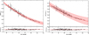 |
Fig. 9 Stellar radius (ℛ, left) and mass (ℳ, right) as a function of the absolute magnitude (MG) valid in the M-dwarf domain. The red line represents the polynomial fit described in Table 4, and the red shaded area indicates the 1-σ level of uncertainty. |
 |
Fig. 10 Nomenclature of multiple systems based on the resolution of Gaia DR3 (blue circles) and 2MASS (orange circles). From left to right: ‘A+B’ (resolved in both surveys), ‘AB’ (only resolved in Gaia), ‘(AB)’ (not resolved either in Gaia or 2MASS, but resolved by adaptive optics, lucky imaging, or space imaging), and ‘Aab’ (spectroscopic binaries). Multiple systems can often be a combination of these cases. |
Coefficients for the polynomial fits of G-band absolute magnitudes to masses and radii.
4.3 Description of the systems
Table A.1 displays all the M dwarfs in Carmencita plus their companions (in the case of multiple systems) resolved by Gaia. It contains a total of 2634 rows (2214 M dwarfs in the study sample plus 420 resolved companions) and 131 columns. Its structure is meant to be both human- and machine-readable. For the former, the systems are displayed with one component of the systems resolved by Gaia per row. A few notable cases lack Gaia identification, such as the very bright Capella or the very faint Wolf 1130 B, but they still have their rows assigned in the table. The stars are sorted by right ascension, but ensuring that those that belong to the same system are consecutive, in order of decreasing brightness.
The nomenclature of the system follows the scheme shown in Fig. 10. The primary components (‘A’, or their variations) are the most massive ones of the systems, which are typically the brightest ones. However, white dwarfs are an exception. Although they are dimmer than M-dwarf companions in most cases (see again Fig. 11), white dwarfs are known to be the remnants of late B to early G main sequence stars, which were more massive than M dwarfs. However, for historical reasons, we considered white dwarfs as companions in all the instances found in this work (see more details in Sect. 4.4.2). A comparison of the different surveys (WISE, Gaia, and 2MASS) and techniques (AO, LI, SB), with a focus on their ability to identify resolved binaries, is shown in the upper panel of Fig. 12; the lower panel shows the difference in magnitude (in general, Gaia’s G) as a function of the angular separation. The resolving capabilities of Gaia DR3 do not only depend on the separation, but also on the flux ratio, with considerable difficulty involved in telling individual sources apart with ρ ≲ 0.6 arcsec and ΔG > 0.1 mag. In addition, it is known that the rectangular pixels of Gaia induce a dependence on the position angle between the two stars, influenced by the scanning direction (de Bruijne et al. 2015); however, this fact is alleviated by the large number of transits at different scanning directions.
Figure 12 also helps to shed light on the boundary between ‘close’ and ‘wide’ pairs. These terms are generally defined in a static way, with separations that depend on the context of the study. However, the distinction between close and wide should be dynamic rather than static, based on the detection limits and spatial resolution of the used facilities. A practical definition of wide pairs could be those that can be resolved using natural seeing conditions (1–2arcsec) without the need for advanced techniques such as AO and LI. The 2MASS survey, with a spatial resolution of 2–4 arcsec, can serve as a useful gauge to define these ‘wide’ pairs. In this work, we aim to adhere to this definition. However, the terms ‘wide’ and ‘close’ may occasionally be used to define specific separations, particularly when referencing the literal works of others.
An adapted version of the complete table can be found in the Appendix as Table A.1, which provides: numerical ID for each star and system, Karmn, common name, and GJ identifiers, coordinates, spectral type, multiplicity type (single, part of multiple systems, or new unresolved binary candidates), and availability in other tables of this work. We give a column-by-column description in Table A.6. A comma-separated values (csv) file of the complete table is available on a dedicated GitHub repository12.
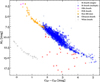 |
Fig. 11 Absolute magnitude MG against GBP − GRP colour for all the stars in our sample and their resolved companions with full photometry available in Gaia DR3. Red crosses correspond to components of multiple systems that are very close, very faint, or both, resulting in compromised photometry. Very bright stars (e.g. Capella or Castor) are necessarily excluded for lacking Gaia photometric measurements. Very compact systems, not resolved by Gaia (Sect. 3.2), and resolved young stars (Sect. 4.5) lie above the main sequence. |
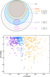 |
Fig. 12 Schematic of the capabilities to identify binaries of the surveys and techniques exploited in this work (top) and difference in G magnitude as a function of angular separation for pairs that Gaia resolves (“AB” or “A+B”) and those for which WDS tabulated magnitude difference (bottom). Both figures follow the same scheme of colours. The nomenclature assigned to each scenario (see again Fig. 10) is also displayed. |
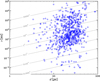 |
Fig. 13 Physical separation as a function of the distance for all the pairs in our sample. The grey dashed lines represent projected angular separations, ρ = s/d, in dex. |
4.3.1 Physical separations
Projected angular separation, p, and projected linear separation, s, relate as s = ρ ⋅ d under the small-angle approximation (sin ρ ≈ ρ, with an error below 1% for ρ < 0.24 radians or 14 deg). The coverage in projected linear separation, s = ρ ⋅ d (or a), of this work extends from 2.810−3 au to 2.7105 au, spanning eight orders of magnitude; namely, from close spectroscopic binaries to ultra-wide systems (Fig. 13). The smallest orbital separation in our sample corresponds to a double-lined spectroscopic binary (SB2), with a minimum value of a sin i = 0.002797 au (1RXS J070005.1–190115, Baroch et al. 2021). On the other hand, the largest orbital separation (273 660 au) corresponds to the widest pair, which is part of a quadruple system (GJ 282 A+B+Cab, Poveda et al. 2009; Baroch et al. 2021) in the Ursa Major stellar kinematic group (Tabernero et al. 2017); therefore, its actual binding may be called into question. The widest pair not associated to any stellar kinematic group is in the quintuple system σ CrB, which consists of three Sun-like main-sequence stars and two low-mass stars: One of them, the M2.5 V σ CrB C star is at 14 346 au to the bright central star.
In terms of angular separation in resolved pairs, the range is 0.020–12 954 arcsec (or 3.6deg). If we extrapolated to non-resolved systems such as SBs, the minimum separation would be as short as 0.0003 arcsec. G 146-35 B is the known equal-mass pair (Lamman et al. 2020) with the smallest angular separation that Gaia DR3 resolves, with just ρ ≈ 0.196 arcsec. Among those reported for the first time, LP 780-23 B is the star (~M3.0V) with the smallest separation from an M dwarf primary, with ρ = 0.199 arcsec. In cases like these, the advantage of being able to resolve the pairs with Gaia comes at the cost of being significantly limited by problems affecting the astrometric measurements. In a few cases we identified members of stellar kinematic groups or associations that were either previously known (therefore confirming their membership) or unknown (therefore assigning them for the first time). These young stars are V1221 Tau with s ≃ 52000 au (in the β Pictoris moving group, Gagné & Faherty 2018), and PM J18542+1058 with s ≃ 10 000 au (primary in the Carina moving group, Gagné & Faherty 2018), proposed for the first time in this work.
In the study of binaries, we faced the problem of translating projected angular separation, ρ, to the actual semimajor axis, a (see e.g. Kuiper 1935; Couteau 1960; van Albada 1968b). For circular orbits, s is always equal or smaller than a; for eccentric orbits, it is the opposite case. The approximation to this problem varies between authors. Many incorporate a fixed correction factor, such as π/2 ≃ 1.57 (Abt & Levy 1976) or 1.26 (Fischer & Marcy 1992, and later Dhital et al. 2010). In contradiction with previous works (e.g. Halbwachs 1983), Torres (1999) suggested that this factor varies with eccentricity. Dupuy & Liu (2011) incorporated this notion (as well as a discovery bias) to yield a factor of  . Other investigations have supported the assumption that s serves as a reasonable estimate for a when there is not enough information about the orbital elements of the system. For instance, Kuiper (1942) derived empirically, from 62 known orbits, a relation between the semimajor axis and the projected separation on the sky that E(log a) − E(log s) = −0.11, where E indicates the expectation value. A similar result was later obtained by Couteau (1960) using 410 orbits. When the eccentricity is taken into account, van Albada (1968b) calculated the expectation values between 0.0 (for e = 1) and −0.133 (for e = 0). More recently, Jiang & Tremaine (2010) stated that for a population of binaries at a given a, the median projected separation is 0.978a. Given the broad scope intended for this work (we refer to the title) and the need for a proper comparison with previous work, we did not apply a conversion factor between a and s, while also assuming random orbital plane orientations.
4.3.2 Öpik’s law
It has been observed in a variety of ranges of separation that the number of pairs per unit of logarithmic separation remains roughly constant (Öpik 1924; Vereshchagin et al. 1988; Close et al. 1990; Allen et al. 2000; Poveda & Allen 2004; Poveda et al. 2007; Lépine & Bongiorno 2007). This empirical relation, often referred to as Öpik’s law, captures the intuitive idea that the probability of finding a bound companion decreases as we go to larger separations. It admits different formulations, either through the frequency distribution f(a) ∝ a−1 or f(s) ∝ s−1, or via the cumulative distribution, which increases linearly on a log-arithmic scale N(log a) ∝ log a or N(log s) ∝ log s, where a and s can be used indistinctly (e.g. Allen et al. 2000).
We show in Fig. 14 the cumulative (top panel) and non-cumulative (bottom panel) distributions of projected physical separations between pairs in our sample. These data include all the possible separations between the elements in each system, namely, n − 1 measurements for a system of n components. We fit two well-sampled ranges in the cumulative distribution, delimited by vertical dashed lines, in which the number of multiple stars is uniformly distributed, separated by a change in slope at s ~ 80 au. We did not make any assumption on the optimal fitting intervals beforehand. Rather, we chose the optimal limits based on the maximisation of the χ2 value. Following Öpik’s law, which states that there are roughly equal numbers of binaries (n0) in each logarithmic interval of s, we expressed the parametrisation as:
 (6)
(6)
where s0 corresponds to the smallest s value in each range, and C and n0 are free parameters. Obtaining very discrepant values for these parameters between both ranges points to a break in Öpik’s law. This behaviour had been already described (e.g. Lépine & Bongiorno 2007), with variations observed across studies due to differences in population characteristics, sample size, and data completeness. For instance, Allen et al. (2000) found that ‘wide binaries’ (a > 25 au, as defined by the authors) follow Öpik’s law all the way up to 10 000 au (and up to 20 000 au for those with the most halo-like orbits). Meanwhile, Poveda et al. (2007) found binaries in the field following Öpik’s law in the separation range 100 au ≤ a ≤ 3000 au, which corresponds to the second range in our plot.
The cumulative distribution shown in Fig. 14 departs from Öpik’s at very close (s ≲ 1 au) and very wide (s ≳ 104 au) orbital separations, a fact repeatedly observed in empirical studies (e.g. Poveda & Allen 2004, but see Poveda et al. 2007 for the exception of very young populations of binaries). The upper limit of Öpik’s law decreases with increasing system age as older systems tend to have fewer wide binaries, simply because they have had more time to be disrupted (see e.g. Weinberg et al. 1987). More recently, King et al. (2012), who studied the separation distributions in young star-forming regions, found an excess of binaries with s < 100 au when compared to the field population. As Lépine & Bongiorno (2007) pointed out that even if a population initially follows the canonical form of Öpik’s law, it will eventually exhibit a truncated distribution with a steeper power law, f (s) ∝ s−λ, where λ > 1.
It has been argued (e.g. Allen et al. 1997) that it might be preferable to describe this distribution function in accordance with the two main mechanisms of binary formation: disk fragmentation for the close systems, and first-collapse (or turbulent) fragmentation or the dynamical unfolding of compact triples for wider systems. Some authors (e.g. El-Badry & Rix 2018; Tian et al. 2020) have adopted a ‘broken’ power law instead. The existence of two formation mechanisms dominating in different separation regimes was also suggested by Tokovinin (2020) and Hwang et al. (2022) when studying the distribution of eccentricities. This observational result alleviates the problem that a single theory (namely, disk fragmentation) faces when explaining the existence of binaries with very wide separations. This behaviour has been observed both in pre-main and in main sequence stars (Poveda 1988; Poveda et al. 1982, 1994; Poveda & Allen 2004). All in all, it is accepted that multiple systems are formed through different processes and that the statistical properties of these systems are influenced by the environment in which they form.
The broad peak around 20 au (Fig. 14, bottom panel) was identified by Winters et al. (2019a), who noted that many stars could potentially harbour close companions, eventually altering the multiplicity rate and shifting the most common separations to smaller orbital sizes, once their orbital semimajor axes are determined. For 89 unresolved systems they adopted fixed projected separations of 1 arsec, which substantially underestimate the number of very close companions (at sub-Solar System scales, or less than 1 au). The authors noted that their distribution figures differed from that of Janson et al. (2014a), but highlighted the methodological differences between the two; this specifically includes the primary mass (Janson et al. 2014a focussed on M5– 9 V). Our study cannot be compared directly with those above, since our distribution cannot be described with a single Gaussian given the broad range of separations that we cover.
Regarding the observed flattening of the distribution at very short and very wide separations, we assert that the former is caused by a fundamental limitation of the main high-resolution techniques (AO, LI, SI), while the latter is a consequence of the difficulty of the formation and eventual survival of the most separated binary systems, rather than observational constraints (see e.g. Poveda & Allen 2004; Lépine & Bongiorno 2007; Caballero 2009; González-Payo et al. 2023). Indeed, Gaia DR3 is complete for separations above 1.5–2.0 arcsec (Fabricius et al. 2021) and so, we did not expect to miss the most separated binaries in our search. The evidence shows that in binaries of a ≲ 50 au, disruption by dyamical influences is negligible. They evolve essentially unaffected, either in the field or inside clusters (see e.g. Moeckel & Bate 2010). Parker et al. (2009) referred to these close-in pairs as ‘hard binaries’, while ‘intermediate binaries’ was used to refer to those with 50 au < a < 1000 au; the latter are severely affected by dynamical processes, especially when formed in dense star clusters. Unevolved ‘wide binaries’ with s > 1000 au can only originate in low-density star-forming regions with less than a few stars per cubic parsec (‘isolated star formation mode’, Goodwin 2010) or, in the words of Deacon & Kraus (2020), ‘wide binaries are rare in open clusters’. Early investigations, such as those by van Albada (1968a), suggested that binaries observed at separations greater than about 1000 au must be either ‘escaping’ double stars (or run-away stars; see also Poveda et al. 1967) or one of the components is actually a double star (yielding to a triple system) that supplies more mass (and therefore more gravitational support) to the system (Reipurth & Mikkola 2012; Cifuentes et al. 2021).
The non-cumulative distribution (Fig. 14, bottom panel) exhibits a rather bimodal shape, peaking at ∼10–100 au and around ∼103 au, respectively, which roughly correspond to the changes in slope in the cumulative distribution, as marked by the range boundaries. It also shows that a large percentage of M dwarf companions are found to be as close as s ≲ 50 au. Studies such as Hwang (2023) found that the fraction of wide (103– 104 au) triple systems increases with decreasing orbital periods of the inner binaries, and the authors also found a tentative excess at ∼104 au for tertiaries of eclipsing binaries. The bimodality in this distribution of separations has been reported before in the literature for wide (s > 103 au) binaries (e.g. Dhital et al. 2010; Oelkers et al. 2017; Jiménez-Esteban et al. 2019) and also for close (<103 au) binaries (Kouwenhoven et al. 2010, see their Fig. 8). Dhital et al. (2010) suggested that this bimodality most likely reveals two distinct populations of wide binaries, possibly representing systems that form or dissipate through differing mechanisms: (1) systems of stars that formed with sufficient binding energy to survive for the age of the Galaxy, and (2) relatively young systems that formed within the past 1–2 Ga but that are not likely to survive much longer. The authors noted their high confidence that the bimodal structure is not due to a large contamination of very wide chance pairs, but likely that this bimodality reveals these two distinct populations of wide binaries. Oelkers et al. (2017) noted that the bimodality is split near separations of 104.7 au, also suggesting two separate binary populations, which follow different formation and evolutionary paths. Using Gaia DR2 data, Jiménez-Esteban et al. (2019) correlated the number of false positives with the separation of the system, estimating that it is ∼1–5% of the candidate pairs with s < 50 000 au, ~10–18% for s between 50 000 and 100 000 au, and increasing to ∼40–51% for the largest separations, therefore resulting in most of their comoving candidate binaries with s ≲104 au being real.
Before the Gaia mission, only relatively small samples of nearby and bright stars had useful parallaxes. Foundational works such as Kuiper (1942) only had limited data available, but recognised the limitations due to the ‘incomplete discoveries of spectroscopic and close visual binaries’ [sic]. More recently, Lépine & Bongiorno (2007) suggested that, using CCD imaging and AO, it should be possible to perform a complete census of common proper motion companions of Hipparcos stars down to angular separations of a fraction of an arcsecond, underlining the usefulness in extending the census to pairs with smaller orbital separations (s < 1000 au) and verify whether this regime can be consistently modelled with Öpik’s law.
Pre-Gaia investigations were fundamentally limited by the astrometric accuracy (in distance measurements and proper motion data), which made the characterisation of binary stars much more challenging. For example, the SLoWPoKES catalogues I and II (Dhital et al. 2010, 2015) were based on Sloan Digital Sky Survey (SDSS) data limited by their use of distance–colour relations rather than direct distance measurements. The SLoWPoKES extension catalogue, GAMBLES (Oelkers et al. 2017), used the published distances and proper motions from the Tycho-Gaia Astrometric Solution (TGAS), which was based on the first data release of Gaia and on the Tycho-2 catalogue, although also relied on SDSS data. TGAS uncertainties are typically around 0.3 mas a−1, with positional uncertainties around 1–2 mas. Gaia DR3 significantly improved these measurements, with typical uncertainties for parallaxes around 0.02–0.03 mas, and 0.01–0.02 mas for positional measurements. Recent catalogues have used Gaia DR1 (Oh et al. 2017), DR2 (Tian et al. 2020; Harris et al. 2020), and EDR3 (El-Badry et al. 2021), which compile hundreds of thousands of pairs with different levels of contamination by chance alignments, sometimes using Bayesian formulation in the process.
Also using TGAS astrometry, Andrews et al. (2017) recognised that the excess of the distribution at s ∼ 104 au corresponds to the transition from genuine binaries to random alignments, implying that the reported bimodality within separations of 1 pc in samples of wide binaries is most likely due to contamination from random alignments. El-Badry et al. (2021) showed that the contamination rate from chance alignments increases rapidly with separation. For instance, they distinguished between ‘initial candidate pairs’ and ‘high bound probability pairs’ (see their Fig. 2), suggesting that most initial candidates are chance alignments, which dominate at s ≳ 3000 au. They concluded that the separation distribution of binaries with high probability of being bound falls off steeply at wide separations. In particular, they suggested that at wide separations (meaning 104.5 au) most candidates are chance alignments, an observation already made by Tian et al. (2020) relying on data from Gaia DR2 (see their Fig. 4). Prior to that study, the results from detailed works on the probabilities of chance alignments by Lépine & Bongiorno (2007) displayed an agreement with these results. By using astrometric data with unprecedented accuracy, the evidence presented here (see Sect. 4.3.4 for the study of binding energies and see again Figure 14) also suggests that some of the ultra-wide binaries ( s ≳ 104 au) claimed to be genuine are, in fact, random alignments.
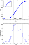 |
Fig. 14 Cumulative (top) and non-cumulative (bottom) distribution of physical separations for all the pairs in our sample. The white dashed lines in the upper panel are power-law fits for the ranges 7–80 au and 80–3000 au, respectively. The grey vertical dashed lines delimit these ranges. |
4.3.3 Orbital periods
Orbital periods (Porb) relate to the semimajor axis, a, and the total mass of the system, ℳT, via Kepler’s third law:
 (7)
(7)
As stated above, the impact of the correction factor between a and s can be neglected. As mentioned in Sect. 1, close compact arrangements of stars can be adequately treated as a single star (with the aggregated masses) when considered from a distance much larger than the separation between its components. In this sense, triple, quadruple, or even higher order systems can be treated as binaries in the majority of cases. Therefore, we estimated orbital periods of the pairs in our sample only for the systems with available masses for all the components, either measured dynamically in the past or estimated by us (see Sect. 4.2), and with the suitable hierarchical arrangement.
Almost all the estimated Porb lie between 10 a and 105 a, with 40% of the total corresponding to periods of less than 103 a (given the dependence of Porb on s, we omit the corresponding histogram, but the bottom panel of Fig. 14 may serve as a representative plot). Without the information about their orbital eccentricity and orientation, these values could be over- as well as under-estimated. For the vast majority of pairs in our sample, the orbital periods are measured by millennia, so the prospect of following them during one single orbit is unrealistic in practice. As an example, we refer again to Proxima Centauri, which has an estimated orbital period Porb ∼ 5.5 · 105 a (Kervella et al. 2017). One consequence is that, in most cases, it will not be possible to discriminate among actual bound multiple systems and disintegrating clusters.
The largest orbital periods estimated correspond to GJ 1284 and GJ 282 C, with extreme values of ∼108 a. On the other hand, several systems have estimated periods of less than half a century. Table 5 lists these systems, along with their masses and separations, both at the epoch of Gaia and at the time of the first satisfactory observation as listed by the WDS. In all cases these systems are binaries resolved by Gaia with angular separations ρ ≲ 2 arcsec. One exception could be the system GJ 400, which might be a triple system made of HO 532 (shown in Table 5) and the innermost CHR 191 (ρ ∼ 0.37 arcsec), but that has been poorly investigated (McAlister et al. 1987). If the system were triple, the orbital period would be of about 20 a.
In addition to the periods estimated by us, we also collected those reported in the literature, mainly derived from the study of spectroscopic binaries. Most of these are measured by days, or even by hours, such as that of LP 86-173 (LHS 1817), an M4.5- dwarf in a 7 h orbit with a possible white dwarf (Newton et al. 2016; Winters et al. 2020). The periods computed by us, as well as those collected from the literature, are included in the full version of Table A.1 (see Sect. 4.3).
4.3.4 Binding energies
The gravitational binding energy of a binary system is a measure of the strength of their attachment. In this sense, Heggie (1975) introduced the categories ‘soft’ and ‘hard’ binaries as a broad classification for the class of attachment that stellar pairs can experience: The former are fragile and easy to break, while the latter are highly resilient to encounters. These definitions resemble those of ‘intermediate’ and ‘hard’ binaries as used by Parker et al. (2009) and summarised in Sect. 4.3.2. The reduced binding energy of a binary system of masses ℳ1 and ℳ2 , with a projected physical separation s, can be written as Caballero (2009):
 (8)
(8)
where the asterisk denotes the use of projected separation instead of the actual one, r, as the latter is unknown in most cases. Given that always r ≥ s, the computed  values represent upper limits to the actual binding energies. Eq. (8) also applies for triple and higher order systems, with ℳ1 and ℳ2 corresponding to aggregated masses. This is, binding energies of high-order systems can be computed as long as they dynamically behave like a binary (as we proceeded when estimating the orbital periods). Figure 15 shows s and
  as a function of the total stellar mass, ℳT = ℳ1 + ℳ2, in the top and bottom panels, respectively.
The dynamical evolution of the stars over time, determined by their environment, sets a time limit for the stability of multiple systems, especially in the case of the most separated pairs. For example, El-Badry & Rix (2018) suggested that most wide binaries with separations exceeding a few thousand au may become unbound during post-main sequence evolution. However, a binary never decays without neighbours. While catastrophic encounters such as collisions are not common, there is a myriad of subtle chances to disrupt their balance. The gravitational interaction with nearby stars can be disruptive in the long term, as shown by Weinberg et al. (1987). Considering the encounters with stars, the estimated average lifetime of a binary (Eq. 28 of their work) is:
 (9)
(9)
where n* and ℳ* account for number density and mass of stellar perturbers, Vrel is the relative velocity between the binary and the perturber, ℳT and a refer to the total mass and semimajor axis of the binary, and Λ is the Coulomb logarithm. The expression accounts for the stochastic gravitational perturbations and the encounters with passing stars. Assuming an average perturber mass of 0.7 ℳ⊙, Vrel = 20 km s−1, Λ = 1, and using the average Galactic disk mass density of 0.11 ℳ⊙ pc−3 (Close et al. 2007; Dhital et al. 2010), Eq. (9) can be greatly simplified as:
 (10)
(10)
Here, smax represents the maximum separation for a total mass ℳT in solar masses, to survive for a given age t⋆ in gigayears. The separations that correspond to ages of 1, 10, and 100 Ga are plotted in Fig. 15.
Parker et al. (2009) suggested that in high- to moderatedensity environments, most binaries with separations ranging from a few hundred to a few thousand au are disrupted within a few million years. Conversely, in lower density regions, galactic tides and weak interactions with passing stars gradually separate binaries with separations of around 104 au over approximately 10 Ga (Heggie 1975; Weinberg et al. 1987). The majority of pairs, separated some dozens or hundreds of au, are expected to be stable for hundreds of gigayears, assuming a negligible occurrence of catastrophic encounters. However, there are eight pairs in our sample with expected survival periods ranging from 1 Ga to 10 Ga. Among them there are the most weakly bound systems, with  , highlighted in red in both panels of Fig. 15. The smallest binding energy, of
  , corresponds to LP 404–54, a resolved component of the M3.5 dwarf primary GJ 3022 at an orbital separation of 60 680 au in a hierarchical triple system. These configurations are remarkably fragile and, therefore, more susceptible to be unbound by dynamical encounters with a plethora of sources of perturbation, such as stars, molecular clouds, clusters, and even stellar-mass black holes (Hills 1975; Retterer & King 1982; Weinberg et al. 1987; Jiang & Tremaine 2010; Parker et al. 2011; Deacon & Kraus 2020; Ryu et al. 2022).
During our search for physical pairs resolved with Gaia up to 105 au, we found some physically bound components with s > 104 au. There are 24 systems with at least one companion of this kind in our sample. Among them there are the eight pairs with the most fragile bindings  , as defined above. They are collected in Table A.7, along with the most relevant parameters. Two of them (V1221 Tau and PMJ18542+1058) are identified as comoving pairs in this work for the first time (see also Table A.3). Among them, PM J18542+1058 is assigned by us as a new member of the Carina association.
Systems with estimated minimum orbital periods of less than 50 years.
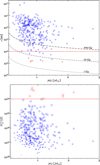 |
Fig. 15 Physical separation (top) and binding energy (bottom) as a function of system total mass. In the bottom panel, sizes are proportional to the physical separation from the primary. Red open circles highlight in both panels the most fragile pairs ( |

4.3.5 Mass ratios
The mass ratio is defined as the fraction q = ℳB/ℳA, where ‘A’ refers to the primary component and ‘B’ refers generically to the remaining components. Given that a large number of the masses of the components of multiple systems are known or, in most cases, estimated when possible (see Sect. 4.2), we were able to calculate q for a considerable fraction of the pairs. We did not compute mass ratios for the M dwarf-white dwarf pairs (Sect. 4.4.2), given the special nature of these configurations, in which one of the components has lost much of its mass during the post-main-sequence evolution. Moreover, many q values involving spectroscopic binaries in one of the components may be absent given that only lower limits of the mass of the SB are often available.
The top panel of Fig. 16 displays the mass ratios of 424 pairs as a function of the physical separation and the primary mass13 . An absence of small q for small primary masses (bottom right corner in the panel) has been observed in previous studies (e.g. Bergfors et al. 2010; Janson et al. 2012; Cortés-Contreras et al. 2017). This is arguably an observational bias, either because most surveys systematically miss either the least massive (faintest) companions (ℳ ≲ 0.1 ℳ⊙) or the most compact binaries (a ≲ 10 au).
In the bottom panel of Fig. 16, the latter observational selection effect is visible, with a remarkable scarcity of data for the closest pairs. This lack of information prevents from testing if near equal-mass pairs (q ≳ 0.8) are typically found at smaller separations (Jódar et al. 2013; Janson et al. 2014b), or if on the contrary mass ratio distributions are independent of separation (Duquennoy & Mayor 1991; Fischer & Marcy 1992; Reggiani & Meyer 2011). Nevertheless, based on the analysis of high-resolution images of 201 nearby systems collected with the Hubble Space Telescope, Dieterich et al. (2012) showed that the mass ratios of low-mass binaries tend to approach to unity as masses approach the hydrogen burning limit at about 0.07 ℳ⊙, which means that brown dwarf companions are scarce. Studies involving the mass-ratio distribution in M dwarf binaries suggest that the formation mechanisms might differ from those of more massive stars, potentially involving more complex interactions and accretion processes (we refer to several of the studies in Table 1). In this sense, we are unable to reproduce the results by Goldberg et al. (2003), who analysed 162 SBs and observed two distinct populations (q ~ 0.2 and q ~ 0.8). But similarly to Winters et al. (2019a), we found no preference for equal-mass systems. When complemented with other orbital parameters, q also conveys important information regarding the long-term dynamical stability of these systems.
In both panels of Fig. 16, some values of q are slightly larger than unity, which at first glance seems contradictory. The most plausible reason has to do with the definition of primary (component ‘A’) as the brightest in the Gaia G magnitude that we followed in this work. This definition can disagree with the original nomenclature of some systems, which based this naming convention typically in Johnson V filter, a narrower passband in comparison with Gaia’s. Another reason could involve a secondary that is actually a binary system of two equal-mass stars, which together could indeed be more massive than the primary, but a more detailed investigation of these secondaries is needed to clarify this hypothesis.
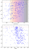 |
Fig. 16 Mass ratios as a function of primary star mass (top) and projected physical separation (bottom), only for M-dwarf primaries. The red dashed line marks q = 1. The gradient map in the background represents the spectral types from M0.0 V to M9.0 V (Cifuentes et al. 2020) following the same scheme as in Fig. 1. |
Companions to M dwarfs found in our sample.
4.4 Companions to M dwarfs
M dwarfs can be found with a variety of stellar and substel- lar companions, ranging from massive OBA stars to ultra-cool dwarfs and planets. In particular, in our sample, only two M dwarfs are companions to A-type stars: Castor, an A1 V spectroscopic binary in a hierarchical sextuple system, and τ07 Ser, an A8 V star in a triple system. There are no earlier OB-type primaries. This lack of OBA+M systems is a direct consequence of the initial mass function and the short life of massive stars in the main sequence. The vast majority of M dwarfs in our sample (around 93%) are found to be paired with other M dwarfs. Table 6 displays a summary of the different types of companions to our M dwarfs. A given system can harbour more than one type of companion. We describe below the systems with FGK- type primaries, white and ultra-cool dwarf companions, and, for completeness, exoplanets.
4.4.1 FGK primaries
Modelling the atmospheres of a star is a challenging task, and the cooler the star, the harder it becomes (see e.g. Valenti et al. 1998; Woolf & Wallerstein 2006; Önehag et al. 2012). Consequently, advances in new grids of theoretical models (MARCS: Gustafsson et al. 1975, 2008 – PHOENIX: Hauschildt et al. 1997; Husser et al. 2013 – NextGen: Hauschildt et al. 1999 – BT-Settl: Baraffe et al. 1998; Allard et al. 2012), lists of atomic and molecular lines and opacities, computational efficiency, and high-resolution spectroscopy are needed to determine effective temperatures, surface gravities, and, especially, element abundances. Gaining precision in the determination of stellar abundances is important for various reasons, including better constrains on planet formation, mantle composition, and relative core size (Dorn et al. 2017). As a result, the CARMENES Consortium has devoted efforts in the precise determination of abundances in M dwarfs (Abia et al. 2020; Marfil et al. 2021; Passegger et al. 2022; Tabernero et al. 2024).
In this effort of calibrating the metallicity of the coolest stars, solar-type physical companions can provide a shortcut because their abundances are much easier to determine (Nordström et al. 2004; Adibekyan et al. 2012; Benítez et al. 2014). A few investigations have estimated M-dwarf metallicities using wide binary pairs with FGK primaries (e.g. Rojas-Ayala et al. 2012; Montes et al. 2018; Birky et al. 2020; Ishikawa et al. 2022; Lim et al. 2024). Among them, Montes et al. (2018) presented a relatively large sample of 192 wide visual binaries covering a reasonably broad range in metallicity and spectral type, with atmospheric parameters of the primaries homogeneously derived with the StePar code (Tabernero et al. 2019), and chemical abundances for 13 atomic species. We expect the list of investigated systems and species to increase in the near future, partly because of this work.
In Table A.8, we list 60 systems that contain 64 stars with spectral types between F5 and K5, and 70 M-dwarf companions. Earlier F and later K stars are either too hot or too cool for precise abundance determinations. Besides, the FGK stars are either dwarfs (60) or giants and subgiants (7). We tabulate the systems, their main astrometric properties, and their iron abundance ([Fe/H] as a proxy of metallicity) from the literature. The abundances of some FGK+M systems in Table A.8 were investigated for the first time by Duque-Arribas et al. (2023).
4.4.2 White dwarfs
White dwarfs (WDs) are remnants of stars less massive than 8–10 ℳ⊙ and represent the final evolutionary stage for the majority of the stars in the Milky Way (Fontaine et al. 2001; Catalán et al. 2008; Doherty et al. 2015). When physically paired with M dwarfs, WDs are a valuable source of information because their modelling is easier (Bergeron et al. 1995; Renedo et al. 2010). For instance, WD companions can serve as effective chronometers for their hosts (Monteiro et al. 2006; Fouesneau et al. 2019; Qiu et al. 2021; Kiman et al. 2021) because the age estimation for WDs is based on their cooling, which is governed by well-understood physics, but one has to add the main-sequence life of the progenitor to get the total age (see Soderblom 2010).
The white dwarfs observed today are probably the remnants of F to late-B main sequence stars (~ 1.2–8 ℳ⊙), with the number of cool unevolved dwarf companions peaking at mid-M type (Farihi et al. 2005). M dwarfs are the most common type of star, yet they do not seem to often pair with white dwarfs. According to Ferrario (2012), this might indicate that the way binary star systems form tends to avoid pairing them with stars that were originally F to late B-type stars. Regarding this observed deficit, Williams (2004) suggested that a large portion of the missing white dwarfs might be explained if these are part of unresolved systems (e.g. Morales-Rueda et al. 2005; Toonen et al. 2017). Ferrario (2012) estimated that there must be an additional ~30% of as yet undiscovered white dwarfs hidden within some kind of binaries. Also, studying wide binary systems from the Sloan Digital Sky Survey, Ferrario (2012) noted that if both M dwarfs and white dwarfs were drawn from the same initial mass function, the number of such systems would be significantly higher than observed, suggesting a different distribution of masses for M dwarf companions. Due to the limited number of WD+M systems, this specific aspect is not addressed in the present work (refer to Sect. 4.3.1).
Table A.9 displays the 28 systems in our sample that have at least one WD component, namely 21 binaries, 6 triples, and 1 quadruple. We tabulate ρ and θ with respect to the WD, as the progenitor was originally the most massive and, thus, brightest, star in the system. The quadruple system contains two white dwarfs (G 107–70 A and G 107–70 B, Limoges et al. 2015) and a resolved (ρ ~ 105 arcsec) equal-mass M4 V binary companion (GJ 275.2 AB, Giclas et al. 1961). Among the triple systems is o02 Eri B, arguably the first white dwarf discovered (Adams 1914; Holberg 2005, and refer to the previous foundational work by Russell and Hertzprung). It orbits the solar-type star o02 Eri A in close binarity with the M4.5 dwarf DY Eri (or o02 Eri C; Herschel 1785).
The object Gaia DR3 2005884249925303168, a physical companion of the M0.0V star LF 4+54 152, is several magnitudes fainter than a main-sequence star of the same colour based on its position in the Hertzsprung-Russell diagram (Fig. 11). Although it has not been spectroscopically confirmed, Jiménez-Esteban et al. (2018) and Gentile Fusillo et al. (2019) classified it as an astro-photometric WD candidate, as we also do. All the remaining WDs have been spectroscopically investigated, and many of them are tabulated by the Montreal White Dwarf Database14 (MWDD). Masses, luminosities, and effective temperatures from evolutionary models are available for several of them in the MWDD, which we retrieved and incorporated in our study.
There have been several observational claims on the projected physical separation distribution of stellar systems with WDs. For example, El-Badry & Rix (2018) suggested that the distribution of s of systems of WDs and main-sequence stars breaks at ~3000 au, twice the break of WD+WD pairs. Unfortunately, the population of binaries in our sample is not sufficiently large to perform an analogous study (there are only five systems with s > 3000 au), but will allow to determine ages complementary to the kinematic study of Cortés-Contreras et al. (2024).
4.4.3 Ultra-cool dwarfs
Ultra-cool dwarfs (UCDs) are a mixture of very low-mass stars and brown dwarfs with spectral types M7.0 V and later. UCDs can provide important insights into the formation and evolution of low-mass stars and brown dwarfs, and can also help quantifying properties such as masses and ages, eventually testing the accuracy of ultra-cool evolutionary models.
In our sample, there are 16 systems with M dwarfs and UCDs, shown in Table A. 10. The spectral types of the UCDs were taken from the literature, except for five, which we derived from G-band absolute magnitudes and the relationships of Cifuentes et al. (2020) and Pecaut & Mamajek (2013). The list of UCDs contains 1 late-M-, 7 L-, and 8 T-type UCDs, including the cornerstone late T8.0–8.5 dwarfs Ross 458C (Wolf 462 C), GJ 570 D, Wolf 1130 B, and Wolf 940 B, which were not detected in our Gaia search. Projected physical separations vary from roughly 25 au of the GJ 9492 system to over 3000 au of the Wolf 1130 AB system.
We provide astrometric measurements of two pairs for the first time: an ~L4 dwarf at just ~0.53 arcsec to the X-ray M2.0 V star 1RXS J190405.9+211030, and an ~L2 dwarf at ~11 arcsec to the M3.0+M3.5: double star LP 395–8 AB. The ~L2 dwarf is reported here for the first time, while the ~L4 dwarf would need an independent astrometric confirmation given its close separation to the brighter primary and lack of five-parameter Gaia solution.
Our collection of systems is smaller than the recent and comprehensive work by Baig et al. (2024), who compiled 278 systems with UCDs at d < 100 pc, or the encyclopedic work by Kirkpatrick et al. (2024), who tabulated all known UCDs (either single or in multiple systems) at d < 20 pc. However, all primaries in Table A.10 (except for the system containing GJ 570 D, whose primary is a K4 V star – Table A.8) are nearby, bright, Carmencita M dwarfs, some of them with CARMENES monitoring and, therefore, high signal-to-noise ratio, high-resolution spectroscopy. As a result, our collection of systems with well- investigated M dwarfs and UCDs can be of help for forthcoming ultra-cool studies (metallicity, kinematics, age dating, dynamical mass determination, etc.).
4.4.4 Exoplanets
On one hand, the multiplicity of stars with exoplanets comes with an inherent observational bias (Lillo-Box et al. 2012; Ciardi et al. 2015; Fontanive & Bardalez Gagliuffi 2021; Mulders et al. 2021; González-Payo et al. 2024), although close stellar companions can also modify the formation, migration, or dynamical evolution of planets (Holman & Wiegert 1999; Mathieu et al. 2000; Desidera & Barbieri 2007; Kaib et al. 2013; Kraus et al. 2016). On the other hand, the discovery of exoplanets around M dwarfs is a relatively new topic in astrophysics, since at the end of the first decade of the 21st century only a bunch such systems were known (e.g. GJ 876 bcd – Marcy et al. 1998, 2001; Rivera et al. 2005, GJ 436 b– Butler et al. 2004, GJ 581 bce – Bonfils et al. 2005; Udry et al. 2007; Mayor et al. 2009).
It was only after the advent of new dedicated extreme precision spectrographs (e.g. CARMENES) and the TESS space mission that the ‘M-dwarf Opportunity’ was eventually made possible. Nowadays, there are hundreds of M dwarfs with known exoplanets (e.g. TRAPPIST-1 a–g – Gillon et al. 2016, LTT 1445 A bc – Winters et al. 2019b, GJ 3929 b – Kemmer et al. 2022, GJ 486 b – Trifonov et al. 2021, Barnard b – González Hernández et al. 2024). However, the multiplicity of M dwarfs with exoplanets has not yet been investigated in detail.
Here, we pave the way for future analyses on this topic by compiling the 99 stars in our initial sample that have exoplanets, 91 of which are M dwarfs, 8 are FGK stars (3 of them non-MS stars), and one is a WD (LP 141–14). We list the planet host stars together with the multiplicity status, number of planets, and corresponding references in Table A.11. For building it, we removed those that have been challenged by CARMENES (see Table 5 of Ribas et al. 2023) or by other authors (Brandt et al. 2020; Šubjak et al. 2023). We identified 73 single- and 28 multiplestar planetary systems. The eight FGK stars and one white dwarf with planets but without a Karmn identifier are companions to Carmencita stars. Not by chance, a significant fraction of the exoplanets in multiple systems in Table A.11 were discovered by CARMENES (Reiners et al. 2018; Kaminski et al. 2018; Perger et al. 2019; González-Álvarez et al. 2020, 2021; Kemmer et al. 2020; Nowak et al. 2020; Stock et al. 2020; Kossakowski et al. 2021; Espinoza et al. 2022). This observational bias is due to the careful preparation of the input catalogue, by which only systems with companions at ρ < 5 arcsec that could contaminate the target’s optical fibre aperture were discarded from the RV survey (Cortés-Contreras et al. 2017).
System components with new assigments to SKGs.
4.5 Young systems
Stellar associations and moving groups are loose unbound star agglomerations that contain from dozens to hundreds of stars with a common origin in space (Eggen 1958, 1975; Montes et al. 2001; Zuckerman & Song 2004; Gagné 2024). Since young stars in stellar kinematic groups (SKGs) represent a transitional stage between the original birthplace and the field, so do young multiple stellar systems in SKGs. Likewise, since wide multiple systems are disrupted by the galactic gravitational potential (Bahcall & Soneira 1980; Weinberg et al. 1987), youth is a common characteristic of the widest pairs (e.g. Caballero 2010; Shaya & Olling 2011; González-Payo et al. 2024).
Recently, Cortés-Contreras et al. (2024) characterised the kinematic properties of the CARMENES input catalogue, identified M-dwarf members in the different galactic populations (thin, transition, and thick discs and halo) and in young SKGs, stellar associations, superclusters, and open clusters with ages from 1 Ma to 800 Ma. They used the public codes SteParKin15 (Montes et al. 2001), LACEwING (Riedel et al. 2017), and BANYAN Σ (Malo et al. 2013; Gagné et al. 2018) for the identification. We assigned the same kinematic properties as Cortés-Contreras et al. (2024), and extrapolated them to their physical companions not listed in Carmencita. After cross-matching with the literature, we found 7 new SKG members in 5 systems from this extrapolation. We list them in Table 7 (see Alonso-Floriano et al. 2015 for an extrapolation example in the β Pictoris moving group).
Table 8 summarises the number of stars classified as kinematically young by Cortés-Contreras et al. (2024) that are part of our input sample (Carmencita M dwarfs plus confirmed resolved companions, Ninput) and of multiple systems (Nsystem). Of the 352 young stars in our input sample (ΣNinput,i), flagged in Table A.1 with the corresponding SKG descriptor, a total of 201 are part of multiple systems (ΣNsystem,i). The large corresponding proportion of young multiple systems is due to the our wide angular search radius, which corresponds to projected physical separations of 105 au (~0.5 pc). At these separations, it is difficult to delimit the boundary between relatively close, but unbound, SKG members and actual very wide binaries, especially in the core of the Hyades supercluster, which is the Hyades cluster itself (see the series of papers started by Caballero 2009). As a result, many of the systems in Table 8 should be taken with a grain a salt. However, as discussed in Sect. 4.3.4 and by González-Payo et al. (2024), binding energies above a certain limit (e.g. 1033−1034 J) could discriminate among actually bound systems and coincidental common proper motion pairs in SKGs. Delimiting such a boundary is beyond the scope of this work.
Number of kinematically young stars in multiple systems.
5 Conclusions
In this work, we explore the prevalence of M dwarfs as part of stellar systems based on a comprehensive photometric and astrometric characterisation. We examined individually each of the 2214 stars in the CARMENES input catalogue in search for known and potential physical companions. We identified a total of 835 M dwarfs as part of 720 multiple systems, predominantly binaries. Additionally, we take advantage of the statistical products of Gaia to propose another 327 candidates to binaries. They are found to exhibit astrometric and photometric anomalies compatible with the presence of an unresolved companion. They should be discarded from input target lists of exoplanet searches with forthcoming space missions (Tuchow et al. 2024; Harada et al. 2024; Menti et al. 2024).
Our findings translate into a minimum multiplicity fraction of 27.8%, which is comparable to the binarity rates reported in previous studies of M dwarfs, although differences in methodology and sample make this comparison somewhat nuanced. Despite this, we suggest that the actual multiplicity fraction of M dwarfs may be significantly higher, potentially reaching 40.3%, if all newly proposed binary candidates are confirmed. This revised estimate brings M dwarf multiplicity more in line with the observed rates among Sun-like stars. Further high- resolution spectral and spatial follow-up studies are mandatory to capture the complete population of close companions. All these analyses will also be complemented with Gaia DR4 (second half of 2026) and DR5 (end of 2030).
A number of other conclusions can be derived from our analyses. In our sample a two-slope distribution of projected physical separations may support the idea that distinct formation mechanisms are at play for different separation regimes, as previous investigations have proposed: the wide-separation pairs suggest a population of systems formed through dynamical interactions, while closer binaries may arise from more traditional fragmentation processes. Pre-Gaia investigations of ultra-wide physical pairs heavily relied on photometric distances due to the lack of precise astrometric data. Previous studies, while valuable, have often suggested the existence of a large number of very wide real binaries, but were dominated by chance alignments at s ≳ 104 au. The mass ratio distribution observed in our sample is slightly skewed towards equal-mass systems, compared to binaries of more massive stars; nonetheless, selection biases are likely to make us miss part of the picture. Given the significant binding energies computed for M-dwarf systems that have not been found to be young, they are likely to remain bound over tens of gigayears, enduring through the majority of the Galaxy’s lifetime.
Finally, we identified remarkable systems with M dwarfs that have FGK star, white dwarf, ultra-cool dwarf, and exoplanet companions, and which belong to young stellar kinematic groups or associations. Fort these systems, we provide a homogeneous compilation of fundamental parameters and observables, and a detailed examination of architectures. These diverse pairings provide unique opportunities for deriving characteristics of M dwarfs that would be otherwise inaccessible or difficult to determine in M dwarfs that are single (e.g. ages, element abundances).
While our results are consistent with previous studies in terms of observed binary frequency, separation distributions, and mass ratio trends, they also highlight the need for continued investigation into close companions and the impact of observational biases. We expect that the data gathered in this work will serve as a valuable asset for testing and informing theoretical predictions, and for providing a foundation for future investigations on multiplicity.
Data availability
Tables A.1–A.12 are only available in electronic form at Zenodo. The full version of Table A.1 is available at the CDS via anonymous ftp to cdsarc.cds.unistra.fr (130.79.128.5) or via https://cdsarc.cds.unistra.fr/viz-bin/cat/J/A+A/693/A228, and at the GitHub repository https://github.com/ccifuentesr/CARMENES-IX.
Acknowledgements
We are grateful to X. Delfosse, J. Gagné, C. Reylé, and, especially, A. Tokovinin and the reviewer Z. Zhang for their valuable suggestions, which have greatly enriched our work. We acknowledge financial support from the Agencia Estatal de Investigación of the Ministerio de Ciencia, Innovación y Universidades and the ERDF through projects 2023AT003 (PIE, CSIC) associated to RYC2021-031640-I, CNS2023-144309, PID2023-150468NB-I00, PID2022-137241NB-C4[1:4], PID2021-125627OB-C31, PID2019-107061GB- C61, BES-2017-080769, and the Centre of Excellence “Severo Ochoa” and “María de Maeztu” awards to the Instituto de Astrofísica de Canarias (CEX2019- 000920-S), Instituto de Astrofísica de Andalucía (CEX2021-001131-S), Institut de Ciències de l’Espai (CEX2020-001058-M), and Centro de Astrobiología (MDM-2017-0737). CARMENES is an instrument at the Centro Astronómico Hispano en Andalucía (CAHA) at Calar Alto (Almería, Spain), operated jointly by the Junta de Andalucía and the Instituto de Astrofísica de Andalucía (CSIC). CARMENES was funded by the Max-Planck-Gesellschaft (MPG), the Consejo Superior de Investigaciones Científicas (CSIC), the Ministerio de Economía y Competitividad (MINECO) and the European Regional Development Fund (ERDF) through projects FICTS-2011-02, ICTS-2017-07-CAHA-4, and CAHA16-CE-3978, and the members of the CARMENES Consortium (Max-Planck-Institut für Astronomie, Instituto de Astrofísica de Andalucía, Lan- dessternwarte Königstuhl, Institut de Ciències de l’Espai, Institut für Astrophysik Göttingen, Universidad Complutense de Madrid, Thüringer Landessternwarte Tautenburg, Instituto de Astrofísica de Canarias, Hamburger Sternwarte, Centro de Astrobiología and Centro Astronómico Hispano-Alemán), with additional contributions by the MINECO, the Deutsche Forschungsgemeinschaft through the Major Research Instrumentation Programme and Research Unit FOR2544 “Blue Planets around Red Stars”, the Klaus Tschira Stiftung, the states of Baden- Württemberg and Niedersachsen, and by the Junta de Andalucía. This work has made use of data from the European Space Agency (ESA) mission Gaia (https://www.cosmos.esa.int/gaia), processed by the Gaia Data Processing and Analysis Consortium (DPAC, https://www.cosmos.esa.int/web/gaia/dpac/consortium). Funding for the DPAC has been provided by national institutions, in particular the institutions participating in the Gaia Multilateral Agreement. This publication made use of the Washington Double Star Catalog maintained at the U.S. Naval Observatory, VOSA and the Filter Profile Service developed and maintained by the Spanish Virtual Observatory through grant AYA2017-84089, the SIMBAD database, the Aladin sky atlas, and the VizieR catalogue access tool developed at CDS, Strasbourg Observatory, France, the NASA Exoplanet Archive, which is operated by the California Institute of Technology, under contract with the National Aeronautics and Space Administration under the Exoplanet Exploration Program, and the Python libraries Matplotlib, NumPy, SciPy, Pandas and collection of software packages AstroPy.
References
- Abia, C., Tabernero, H. M., Korotin, S. A., et al. 2020, A&A, 642, A227 [NASA ADS] [CrossRef] [EDP Sciences] [Google Scholar]
- Abt, H. A., & Levy, S. G. 1976, ApJS, 30, 273 [Google Scholar]
- Adams, W. S. 1914, PASP, 26, 198 [NASA ADS] [CrossRef] [Google Scholar]
- Adibekyan, V. Z., Sousa, S. G., Santos, N. C., et al. 2012, A&A, 545, A32 [NASA ADS] [CrossRef] [EDP Sciences] [Google Scholar]
- Allard, F., Homeier, D., & Freytag, B. 2012, Philos. Trans. Roy. Soc. Lond. A, 370, 2765 [NASA ADS] [Google Scholar]
- Allen, C., Poveda, A., & Herrera, M. A. 1997, in Astrophysics and Space Science Library, 223, Visual Double Stars : Formation, Dynamics and Evolutionary Tracks, eds. J. A. Docobo, A. Elipe, & H. McAlister, 133 [NASA ADS] [CrossRef] [Google Scholar]
- Allen, C., Poveda, A., & Herrera, M. A. 2000, A&A, 356, 529 [NASA ADS] [Google Scholar]
- Allison, R. J., & Goodwin, S. P. 2011, MNRAS, 415, 1967 [NASA ADS] [CrossRef] [Google Scholar]
- Alonso-Floriano, F. J., Morales, J. C., Caballero, J. A., et al. 2015, A&A, 577, A128 [NASA ADS] [CrossRef] [EDP Sciences] [Google Scholar]
- Andersen, J. 1991, A&A Rev., 3, 91 [Google Scholar]
- Andrews, J. J., Chanamé, J., & Agüeros, M. A. 2017, MNRAS, 472, 675 [NASA ADS] [CrossRef] [Google Scholar]
- Andrews, J. J., Anguiano, B., Chanamé, J., et al. 2019, ApJ, 871, 42 [NASA ADS] [CrossRef] [Google Scholar]
- Arenou, F., Luri, X., Babusiaux, C., et al. 2018, A&A, 616, A17 [NASA ADS] [CrossRef] [EDP Sciences] [Google Scholar]
- Auvergne, M., Bodin, P., Boisnard, L., et al. 2009, A&A, 506, 411 [NASA ADS] [CrossRef] [EDP Sciences] [Google Scholar]
- Bahcall, J. N., & Soneira, R. M. 1980, ApJS, 44, 73 [NASA ADS] [CrossRef] [Google Scholar]
- Baig, S., Smart, R. L., Jones, H. R. A., et al. 2024, MNRAS, 533, 3784 [Google Scholar]
- Baraffe, I., Chabrier, G., Allard, F., & Hauschildt, P. H. 1998, A&A, 337, 403 [Google Scholar]
- Baroch, D., Morales, J. C., Ribas, I., et al. 2021, A&A, 653, A49 [NASA ADS] [CrossRef] [EDP Sciences] [Google Scholar]
- Basri, G., & Reiners, A. 2006, AJ, 132, 663 [NASA ADS] [CrossRef] [Google Scholar]
- Bate, M. R. 2012, MNRAS, 419, 3115 [NASA ADS] [CrossRef] [Google Scholar]
- Bate, M. R., Bonnell, I. A., & Bromm, V. 2003, MNRAS, 339, 577 [NASA ADS] [CrossRef] [Google Scholar]
- Batten, A. H. 1973, Binary and Multiple Systems of Stars (Pergamon Press) [Google Scholar]
- Bayo, A., Rodrigo, C., Barrado y Navascués, D., et al. 2008, A&A, 492, 277 [NASA ADS] [CrossRef] [EDP Sciences] [Google Scholar]
- Bean, J. L., Benedict, G. F., & Endl, M. 2006, ApJ, 653, L65 [Google Scholar]
- Bédard, A., Bergeron, P., Brassard, P., & Fontaine, G. 2020, ApJ, 901, 93 [Google Scholar]
- Belokurov, V., Penoyre, Z., Oh, S., et al. 2020, MNRAS, 496, 1922 [Google Scholar]
- Benítez, N., Dupke, R., Moles, M., et al. 2014, arXiv e-prints [arXiv:1403.5237] [Google Scholar]
- Bergeron, P., Wesemael, F., & Beauchamp, A. 1995, PASP, 107, 1047 [Google Scholar]
- Bergfors, C., Brandner, W., Janson, M., et al. 2010, A&A, 520, A54 [NASA ADS] [CrossRef] [EDP Sciences] [Google Scholar]
- Birky, J., Hogg, D. W., Mann, A. W., & Burgasser, A. 2020, ApJ, 892, 31 [Google Scholar]
- Bochanski, J. J., Hawley, S. L., Covey, K. R., et al. 2010, AJ, 139, 2679 [NASA ADS] [CrossRef] [Google Scholar]
- Bonfils, X., Forveille, T., Delfosse, X., et al. 2005, A&A, 443, L15 [NASA ADS] [CrossRef] [EDP Sciences] [Google Scholar]
- Bonfils, X., Delfosse, X., Udry, S., et al. 2013, A&A, 549, A109 [NASA ADS] [CrossRef] [EDP Sciences] [Google Scholar]
- Bonnarel, F., Fernique, P., Bienaymé, O., et al. 2000, A&AS, 143, 33 [NASA ADS] [CrossRef] [EDP Sciences] [Google Scholar]
- Bonnell, I. A., Bate, M. R., & Vine, S. G. 2003, MNRAS, 343, 413 [NASA ADS] [CrossRef] [Google Scholar]
- Borucki, W. J., Koch, D., Basri, G., et al. 2010, Science, 327, 977 [Google Scholar]
- Bouy, H., Brandner, W., Martín, E. L., et al. 2003, AJ, 126, 1526 [CrossRef] [Google Scholar]
- Brandt, T. D. 2021, ApJS, 254, 42 [NASA ADS] [CrossRef] [Google Scholar]
- Brandt, T. D., Dupuy, T. J., Bowler, B. P., et al. 2020, AJ, 160, 196 [Google Scholar]
- Burgasser, A. J., Kirkpatrick, J. D., Reid, I. N., et al. 2003, ApJ, 586, 512 [Google Scholar]
- Burgasser, A. J., Reid, I. N., Siegler, N., et al. 2007, in Protostars and Planets V, eds. B. Reipurth, D. Jewitt, & K. Keil, 427 [Google Scholar]
- Butler, R. P., Vogt, S. S., Marcy, G. W., et al. 2004, ApJ, 617, 580 [NASA ADS] [CrossRef] [Google Scholar]
- Caballero, J. A. 2007, A&A, 462, L61 [NASA ADS] [CrossRef] [EDP Sciences] [Google Scholar]
- Caballero, J. A. 2009, A&A, 507, 251 [NASA ADS] [CrossRef] [EDP Sciences] [Google Scholar]
- Caballero, J. A. 2010, A&A, 514, A98 [NASA ADS] [CrossRef] [EDP Sciences] [Google Scholar]
- Caballero, J. A., Montes, D., Klutsch, A., et al. 2010, A&A, 520, A91 [NASA ADS] [CrossRef] [EDP Sciences] [Google Scholar]
- Caballero, J. A., Cortés-Contreras, M., Alonso-Floriano, F. J., et al. 2016, in 19th Cambridge Workshop on Cool Stars, Stellar Systems, and the Sun (CS19), 148 [Google Scholar]
- Caballero, J. A., González-Álvarez, E., Brady, M., et al. 2022, A&A, 665, A120 [NASA ADS] [CrossRef] [EDP Sciences] [Google Scholar]
- Castro-Ginard, A., Penoyre, Z., Casey, A. R., et al. 2024, A&A, 688, A1 [NASA ADS] [CrossRef] [EDP Sciences] [Google Scholar]
- Catalán, S., Isern, J., García-Berro, E., & Ribas, I. 2008, MNRAS, 387, 1693 [Google Scholar]
- Chabrier, G. 2003, PASP, 115, 763 [Google Scholar]
- Chanamé, J., & Gould, A. 2004, ApJ, 601, 289 [CrossRef] [Google Scholar]
- Chanamé, J., & Ramírez, I. 2012, ApJ, 746, 102 [CrossRef] [Google Scholar]
- Chini, R., Hoffmeister, V. H., Nasseri, A., Stahl, O., & Zinnecker, H. 2012, MNRAS, 424, 1925 [Google Scholar]
- Chulkov, D., & Malkov, O. 2022, MNRAS, 517, 2925 [NASA ADS] [CrossRef] [Google Scholar]
- Ciardi, D. R., Beichman, C. A., Horch, E. P., & Howell, S. B. 2015, ApJ, 805, 16 [NASA ADS] [CrossRef] [Google Scholar]
- Cifuentes, C., Caballero, J. A., Cortés-Contreras, M., et al. 2020, A&A, 642, A115 [NASA ADS] [CrossRef] [EDP Sciences] [Google Scholar]
- Cifuentes, C., Caballero, J. A., & Agustí, S. 2021, RNAAS, 5, 129 [Google Scholar]
- Clark, B. M., Blake, C. H., & Knapp, G. R. 2012, ApJ, 744, 119 [NASA ADS] [CrossRef] [Google Scholar]
- Clark, C. A., van Belle, G. T., Horch, E. P., et al. 2022, AJ, 164, 33 [NASA ADS] [CrossRef] [Google Scholar]
- Clark, C. A., van Belle, G. T., Horch, E. P., et al. 2024, AJ, 167, 174 [NASA ADS] [CrossRef] [Google Scholar]
- Close, L. M., Richer, H. B., & Crabtree, D. R. 1990, AJ, 100, 1968 [NASA ADS] [CrossRef] [Google Scholar]
- Close, L. M., Zuckerman, B., Song, I., et al. 2007, ApJ, 660, 1492 [NASA ADS] [CrossRef] [Google Scholar]
- Cortés-Contreras, M., Béjar, V. J. S., Caballero, J. A., et al. 2017, A&A, 597, A47 [NASA ADS] [CrossRef] [EDP Sciences] [Google Scholar]
- Cortés-Contreras, M., Caballero, J. A., Montes, D., et al. 2024, A&A, 692, A206 [NASA ADS] [CrossRef] [EDP Sciences] [Google Scholar]
- Couteau, P. 1960, J. Observateurs, 43, 41 [Google Scholar]
- Cutri, R.M., Wright, E.L., Conrow, T., et al., 2014, VizieR Online Data Catalog II/328 [Google Scholar]
- Czavalinga, D. R., Mitnyan, T., Rappaport, S. A., et al. 2023, A&A, 670, A75 [NASA ADS] [CrossRef] [EDP Sciences] [Google Scholar]
- Dai, F., Howard, A. W., Halverson, S., et al. 2024, AJ, 168, 101 [NASA ADS] [CrossRef] [Google Scholar]
- Deacon, N. R., & Kraus, A. L. 2020, MNRAS, 496, 5176 [NASA ADS] [CrossRef] [Google Scholar]
- de Bruijne, J. H. J., Allen, M., Azaz, S., et al. 2015, A&A, 576, A74 [NASA ADS] [CrossRef] [EDP Sciences] [Google Scholar]
- Delfosse, X., Forveille, T., Beuzit, J. L., et al. 1999, A&A, 344, 897 [NASA ADS] [Google Scholar]
- Delgado-Donate, E. J., Clarke, C. J., & Bate, M. R. 2003, MNRAS, 342, 926 [NASA ADS] [CrossRef] [Google Scholar]
- Desidera, S., & Barbieri, M. 2007, A&A, 462, 345 [NASA ADS] [CrossRef] [EDP Sciences] [Google Scholar]
- Desidera, S., Gratton, R. G., Scuderi, S., et al. 2004, A&A, 420, 683 [NASA ADS] [CrossRef] [EDP Sciences] [Google Scholar]
- Desidera, S., Gratton, R. G., Lucatello, S., & Claudi, R. U. 2006, A&A, 454, 581 [NASA ADS] [CrossRef] [EDP Sciences] [Google Scholar]
- Dhital, S., West, A. A., Stassun, K. G., & Bochanski, J. J. 2010, AJ, 139, 2566 [NASA ADS] [CrossRef] [Google Scholar]
- Dhital, S., West, A. A., Stassun, K. G., Schluns, K. J., & Massey, A. P. 2015, AJ, 150, 57 [NASA ADS] [CrossRef] [Google Scholar]
- Dieterich, S. B., Henry, T. J., Golimowski, D. A., Krist, J. E., & Tanner, A. M. 2012, AJ, 144, 64 [Google Scholar]
- Dittmann, J. A., Irwin, J. M., Charbonneau, D., & Berta-Thompson, Z. K. 2014, ApJ, 784, 156 [NASA ADS] [CrossRef] [Google Scholar]
- Doherty, C. L., Gil-Pons, P., Siess, L., Lattanzio, J. C., & Lau, H. H. B. 2015, MNRAS, 446, 2599 [Google Scholar]
- Dorn, C., Venturini, J., Khan, A., et al. 2017, A&A, 597, A37 [NASA ADS] [CrossRef] [EDP Sciences] [Google Scholar]
- Duchêne, G., & Kraus, A. 2013, ARA&A, 51, 269 [Google Scholar]
- Dupuy, T. J., & Liu, M. C. 2011, ApJ, 733, 122 [NASA ADS] [CrossRef] [Google Scholar]
- Duque-Arribas, C., Montes, D., Tabernero, H. M., et al. 2023, ApJ, 944, 106 [NASA ADS] [CrossRef] [Google Scholar]
- Duquennoy, A., & Mayor, M. 1991, A&A, 248, 485 [NASA ADS] [Google Scholar]
- Eggen, O. J. 1958, MNRAS, 118, 65 [Google Scholar]
- Eggen, O. J. 1975, PASP, 87, 37 [Google Scholar]
- El-Badry, K. 2024, New A Rev., 98, 101694 [NASA ADS] [CrossRef] [Google Scholar]
- El-Badry, K., & Rix, H.-W. 2018, MNRAS, 480, 4884 [Google Scholar]
- El-Badry, K., Rix, H.-W., & Heintz, T. M. 2021, MNRAS, 506, 2269 [NASA ADS] [CrossRef] [Google Scholar]
- Elliott, P., Bayo, A., Melo, C. H. F., et al. 2014, A&A, 568, A26 [NASA ADS] [CrossRef] [EDP Sciences] [Google Scholar]
- Espinoza, N., Pallé, E., Kemmer, J., et al. 2022, AJ, 163, 133 [NASA ADS] [CrossRef] [Google Scholar]
- Evans, D. S. 1968, QJRAS, 9, 388 [NASA ADS] [Google Scholar]
- Eyer, L., Mowlavi, N., Evans, D. W., et al. 2017, arXiv e-prints [arXiv:1702.03295] [Google Scholar]
- Eyer, L., Audard, M., Holl, B., et al. 2023, A&A, 674, A13 [NASA ADS] [CrossRef] [EDP Sciences] [Google Scholar]
- Fabricius, C., Luri, X., Arenou, F., et al. 2021, A&A, 649, A5 [NASA ADS] [CrossRef] [EDP Sciences] [Google Scholar]
- Faherty, J. K., Burgasser, A. J., Walter, F. M., et al. 2012, ApJ, 752, 56 [Google Scholar]
- Farihi, J., Becklin, E. E., & Zuckerman, B. 2005, ApJS, 161, 394 [CrossRef] [Google Scholar]
- Ferrario, L. 2012, MNRAS, 426, 2500 [NASA ADS] [CrossRef] [Google Scholar]
- Finch, C. T., & Zacharias, N. 2016, AJ, 151, 160 [NASA ADS] [CrossRef] [Google Scholar]
- Fischer, D. A., & Marcy, G. W. 1992, ApJ, 396, 178 [NASA ADS] [CrossRef] [Google Scholar]
- Fontaine, G., Brassard, P., & Bergeron, P. 2001, PASP, 113, 409 [NASA ADS] [CrossRef] [Google Scholar]
- Fontanive, C., & Bardalez Gagliuffi, D. 2021, Front. Astron. Space Sci., 8, 16 [NASA ADS] [CrossRef] [Google Scholar]
- Fontanive, C., Biller, B., Bonavita, M., & Allers, K. 2018, MNRAS, 479, 2702 [Google Scholar]
- Fouesneau, M., Rix, H.-W., von Hippel, T., Hogg, D. W., & Tian, H. 2019, ApJ, 870, 9 [Google Scholar]
- Fouqué, P., Moutou, C., Malo, L., et al. 2018, MNRAS, 475, 1960 [Google Scholar]
- Freund, S., Robrade, J., Schneider, P. C., & Schmitt, J. H. M. M. 2020, A&A, 640, A66 [NASA ADS] [CrossRef] [EDP Sciences] [Google Scholar]
- Gagné, J. 2024, PASP, 136, 063001 [Google Scholar]
- Gagné, J., & Faherty, J. K. 2018, ApJ, 862, 138 [Google Scholar]
- Gagné, J., Mamajek, E. E., Malo, L., et al. 2018, ApJ, 856, 23 [Google Scholar]
- Gaia Collaboration (Prusti, T., et al.) 2016, A&A, 595, A1 [NASA ADS] [CrossRef] [EDP Sciences] [Google Scholar]
- Gaia Collaboration (Brown, A. G. A., et al.) 2018, A&A, 616, A1 [NASA ADS] [CrossRef] [EDP Sciences] [Google Scholar]
- Gaia Collaboration (Brown, A. G. A., et al.) 2021a, A&A, 649, A1 [NASA ADS] [CrossRef] [EDP Sciences] [Google Scholar]
- Gaia Collaboration (Smart, R. L., et al.) 2021b, A&A, 649, A6 [EDP Sciences] [Google Scholar]
- Gaia Collaboration (Arenou, F., et al.) 2023a, A&A, 674, A34 [CrossRef] [EDP Sciences] [Google Scholar]
- Gaia Collaboration (Vallenari, A., et al.) 2023b, A&A, 674, A1 [NASA ADS] [CrossRef] [EDP Sciences] [Google Scholar]
- Gandhi, P., Buckley, D. A. H., Charles, P. A., et al. 2022, MNRAS, 510, 3885 [CrossRef] [Google Scholar]
- Garcés, A., Catalán, S., & Ribas, I. 2011, A&A, 531, A7 [NASA ADS] [CrossRef] [EDP Sciences] [Google Scholar]
- Gentile Fusillo, N. P., Tremblay, P.-E., Gänsicke, B. T., et al. 2019, MNRAS, 482, 4570 [Google Scholar]
- Giclas, H. L., Burnham, R., & Thomas, N. G. 1961, Lowell Observ. Bull., 6, 61 [Google Scholar]
- Gillon, M., Jehin, E., Lederer, S. M., et al. 2016, Nature, 533, 221 [Google Scholar]
- Gizis, J. E. 1997, AJ, 113, 806 [NASA ADS] [CrossRef] [Google Scholar]
- Gizis, J. E., Reid, I. N., & Hawley, S. L. 2002, AJ, 123, 3356 [Google Scholar]
- Gliese, W., & Jahreiß, H. 1991, Preliminary Version of the Third Catalogue of Nearby Stars, On: The Astronomical Data Center CD-ROM: Selected Astronomical Catalogs, I, eds. L. E. Brotzmann, & S. E. Gesser (Greenbelt, MD: NASA/Astronomical Data Center, Goddard Space Flight Center) [Google Scholar]
- Goffo, E., Chaturvedi, P., Murgas, F., et al. 2024, A&A, 685, A147 [NASA ADS] [CrossRef] [EDP Sciences] [Google Scholar]
- Goldberg, D., Mazeh, T., & Latham, D. W. 2003, ApJ, 591, 397 [NASA ADS] [CrossRef] [Google Scholar]
- Golovin, A., Reffert, S., Just, A., et al. 2023, A&A, 670, A19 [NASA ADS] [CrossRef] [EDP Sciences] [Google Scholar]
- González-Álvarez, E., Zapatero Osorio, M. R., Caballero, J. A., et al. 2020, A&A, 637, A93 [EDP Sciences] [Google Scholar]
- González-Álvarez, E., Petralia, A., Micela, G., et al. 2021, A&A, 649, A157 [NASA ADS] [CrossRef] [EDP Sciences] [Google Scholar]
- González-Álvarez, E., Zapatero Osorio, M. R., Caballero, J. A., et al. 2023, A&A, 675, A177 [NASA ADS] [CrossRef] [EDP Sciences] [Google Scholar]
- González-Payo, J., Caballero, J. A., & Cortés-Contreras, M. 2023, A&A, 670, A102 [NASA ADS] [CrossRef] [EDP Sciences] [Google Scholar]
- González-Payo, J., Caballero, J. A., Gorgas, J., et al. 2024, A&A, 689, A302 [NASA ADS] [CrossRef] [EDP Sciences] [Google Scholar]
- González Hernández, J. I., Suárez Mascareño, A., Silva, A. M., et al. 2024, A&A, 690, A79 [NASA ADS] [CrossRef] [EDP Sciences] [Google Scholar]
- Goodwin, S. P. 2010, Philos. Trans. Roy. Soc. Lond. A, 368, 851 [NASA ADS] [Google Scholar]
- Goodwin, S. P. 2013, MNRAS, 430, L6 [NASA ADS] [Google Scholar]
- Goodwin, S. P., & Kroupa, P. 2005, A&A, 439, 565 [NASA ADS] [CrossRef] [EDP Sciences] [Google Scholar]
- Goodwin, S. P., Kroupa, P., Goodman, A., & Burkert, A. 2007, in Protostars and Planets V, 133 [Google Scholar]
- GRAVITY Collaboration (Abuter, R., et al.) 2024, A&A, 685, L9 [NASA ADS] [CrossRef] [EDP Sciences] [Google Scholar]
- Gray, R. O., Napier, M. G., & Winkler, L. I. 2001, AJ, 121, 2148 [Google Scholar]
- Gustafsson, B., Bell, R. A., Eriksson, K., & Nordlund, A. 1975, A&A, 42, 407 [NASA ADS] [Google Scholar]
- Gustafsson, B., Edvardsson, B., Eriksson, K., et al. 2008, A&A, 486, 951 [NASA ADS] [CrossRef] [EDP Sciences] [Google Scholar]
- Halbwachs, J. L. 1983, A&A, 128, 399 [NASA ADS] [Google Scholar]
- Harada, C. K., Dressing, C. D., Kane, S. R., & Ardestani, B. A. 2024, ApJS, 272, 30 [NASA ADS] [CrossRef] [Google Scholar]
- Harrington, R. S. 1972, Celest. Mech., 6, 322 [Google Scholar]
- Hartigan, P., Strom, K. M., & Strom, S. E. 1994, ApJ, 427, 961 [NASA ADS] [CrossRef] [Google Scholar]
- Harris, C. R., Millman, K. J., van der Walt, S. J., et al. 2020, Nature, 585, 357 [NASA ADS] [CrossRef] [Google Scholar]
- Hartkopf, W. I., McAlister, H. A., & Mason, B. D. 2001, AJ, 122, 3480 [NASA ADS] [CrossRef] [Google Scholar]
- Hartkopf, W. I., Tokovinin, A., & Mason, B. D. 2012, AJ, 143, 42 [Google Scholar]
- Hartman, Z. D., & Lépine, S. 2020, ApJS, 247, 66 [NASA ADS] [CrossRef] [Google Scholar]
- Hauschildt, P. H., Baron, E., & Allard, F. 1997, ApJ, 483, 390 [Google Scholar]
- Hauschildt, P. H., Allard, F., & Baron, E. 1999, ApJ, 512, 377 [Google Scholar]
- Hawkins, K., Lucey, M., Ting, Y.-S., et al. 2020, MNRAS, 492, 1164 [NASA ADS] [CrossRef] [Google Scholar]
- Heggie, D. C. 1975, MNRAS, 173, 729 [NASA ADS] [CrossRef] [Google Scholar]
- Henry, T. J. 1991, PhD thesis, University of Arizona, USA [Google Scholar]
- Henry, T. J., & McCarthy, D. W. J. 1990, ApJ, 350, 334 [NASA ADS] [CrossRef] [Google Scholar]
- Henry, T. J., Kirkpatrick, J. D., & Simons, D. A. 1994, AJ, 108, 1437 [NASA ADS] [CrossRef] [Google Scholar]
- Henry, T. J., Jao, W.-C., Subasavage, J. P., et al. 2006, AJ, 132, 2360 [Google Scholar]
- Herschel, W. 1785, Philos. Trans. Roy. Soc. Lond. I, 75, 40 [CrossRef] [Google Scholar]
- Hills, J. G. 1975, AJ, 80, 809 [NASA ADS] [CrossRef] [Google Scholar]
- Høg, E., Fabricius, C., Makarov, V. V., et al. 2000, A&A, 355, L27 [Google Scholar]
- Holberg, J. B. 2005, in American Astronomical Society Meeting Abstracts, 207 [Google Scholar]
- Holl, B., Fabricius, C., Portell, J., et al. 2023, A&A, 674, A25 [NASA ADS] [CrossRef] [EDP Sciences] [Google Scholar]
- Holman, M. J., & Wiegert, P. A. 1999, AJ, 117, 621 [Google Scholar]
- Huang, S. S., & Struve, O. 1956, AJ, 61, 300 [NASA ADS] [CrossRef] [Google Scholar]
- Husser, T. O., Wende-von Berg, S., Dreizler, S., et al. 2013, A&A, 553, A6 [NASA ADS] [CrossRef] [EDP Sciences] [Google Scholar]
- Hwang, H.-C. 2023, MNRAS, 518, 1750 [Google Scholar]
- Hwang, H.-C., Ting, Y.-S., & Zakamska, N. L. 2022, MNRAS, 512, 3383 [NASA ADS] [CrossRef] [Google Scholar]
- Ishikawa, H. T., Aoki, W., Hirano, T., et al. 2022, AJ, 163, 72 [NASA ADS] [CrossRef] [Google Scholar]
- Izmailov, I. S. 2019, Astron. Lett., 45, 30 [NASA ADS] [CrossRef] [Google Scholar]
- Jackson, R. J., Deliyannis, C. P., & Jeffries, R. D. 2018, MNRAS, 476, 3245 [NASA ADS] [CrossRef] [Google Scholar]
- Janson, M., Hormuth, F., Bergfors, C., et al. 2012, ApJ, 754, 44 [Google Scholar]
- Janson, M., Bergfors, C., Brandner, W., et al. 2014a, ApJS, 214, 17 [NASA ADS] [CrossRef] [Google Scholar]
- Janson, M., Bergfors, C., Brandner, W., et al. 2014b, ApJ, 789, 102 [Google Scholar]
- Jiang, Y.-F., & Tremaine, S. 2010, MNRAS, 401, 977 [Google Scholar]
- Jiménez-Esteban, F. M., Torres, S., Rebassa-Mansergas, A., et al. 2018, MNRAS, 480, 4505 [Google Scholar]
- Jiménez-Esteban, F. M., Solano, E., & Rodrigo, C. 2019, AJ, 157, 78 [Google Scholar]
- Jódar, E., Pérez-Garrido, A., Díaz-Sánchez, A., et al. 2013, MNRAS, 429, 859 [Google Scholar]
- Joergens, V. 2008, A&A, 492, 545 [NASA ADS] [CrossRef] [EDP Sciences] [Google Scholar]
- Jørgensen, B. R., & Lindegren, L. 2005, A&A, 436, 127 [Google Scholar]
- Joy, A. H., & Sanford, R. F. 1926, ApJ, 64, 250 [NASA ADS] [CrossRef] [Google Scholar]
- Kaib, N. A., Raymond, S. N., & Duncan, M. 2013, Nature, 493, 381 [Google Scholar]
- Kaminski, A., Trifonov, T., Caballero, J. A., et al. 2018, A&A, 618, A115 [NASA ADS] [CrossRef] [EDP Sciences] [Google Scholar]
- Katz, D., Sartoretti, P., Guerrier, A., et al. 2023, A&A, 674, A5 [NASA ADS] [CrossRef] [EDP Sciences] [Google Scholar]
- Kemmer, J., Stock, S., Kossakowski, D., et al. 2020, A&A, 642, A236 [EDP Sciences] [Google Scholar]
- Kemmer, J., Dreizler, S., Kossakowski, D., et al. 2022, A&A, 659, A17 [NASA ADS] [CrossRef] [EDP Sciences] [Google Scholar]
- Kepler, S. O., Kleinman, S. J., Nitta, A., et al. 2007, MNRAS, 375, 1315 [NASA ADS] [CrossRef] [Google Scholar]
- Kervella, P., Thévenin, F., & Lovis, C. 2017, A&A, 598, L7 [NASA ADS] [CrossRef] [EDP Sciences] [Google Scholar]
- Kervella, P., Arenou, F., Mignard, F., & Thévenin, F. 2019, A&A, 623, A72 [NASA ADS] [CrossRef] [EDP Sciences] [Google Scholar]
- Kesseli, A. Y., Muirhead, P. S., Mann, A. W., & Mace, G. 2018, AJ, 155, 225 [Google Scholar]
- Kiman, R., Faherty, J. K., Cruz, K. L., et al. 2021, AJ, 161, 277 [NASA ADS] [CrossRef] [Google Scholar]
- King, R. R., Goodwin, S. P., Parker, R. J., & Patience, J. 2012, MNRAS, 427, 2636 [NASA ADS] [CrossRef] [Google Scholar]
- Kirk, B., Conroy, K., Prša, A., et al. 2016, AJ, 151, 68 [Google Scholar]
- Kirkpatrick, J. D., Henry, T. J., & McCarthy, D. W. J. 1991, ApJS, 77, 417 [NASA ADS] [CrossRef] [Google Scholar]
- Kirkpatrick, J. D., Gelino, C. R., Cushing, M. C., et al. 2012, ApJ, 753, 156 [NASA ADS] [CrossRef] [Google Scholar]
- Kirkpatrick, J. D., Marocco, F., Gelino, C. R., et al. 2024, ApJS, 271, 55 [NASA ADS] [CrossRef] [Google Scholar]
- Kopparapu, R. K., Ramirez, R., Kasting, J. F., et al. 2013, ApJ, 765, 131 [NASA ADS] [CrossRef] [Google Scholar]
- Kossakowski, D., Kemmer, J., Bluhm, P., et al. 2021, A&A, 656, A124 [NASA ADS] [CrossRef] [EDP Sciences] [Google Scholar]
- Kouwenhoven, M. B. N., Brown, A. G. A., Portegies Zwart, S. F., & Kaper, L. 2007, A&A, 474, 77 [NASA ADS] [CrossRef] [EDP Sciences] [Google Scholar]
- Kouwenhoven, M. B. N., Goodwin, S. P., Parker, R. J., et al. 2010, MNRAS, 404, 1835 [NASA ADS] [Google Scholar]
- Kozai, Y. 1962, AJ, 67, 591 [Google Scholar]
- Kraus, A. L., & Hillenbrand, L. A. 2009, ApJ, 704, 531 [Google Scholar]
- Kraus, A. L., Ireland, M. J., Huber, D., Mann, A. W., & Dupuy, T. J. 2016, AJ, 152, 8 [NASA ADS] [CrossRef] [Google Scholar]
- Kroupa, P., Tout, C. A., & Gilmore, G. 1991, MNRAS, 251, 293 [CrossRef] [Google Scholar]
- Kuiper, G. P. 1935, PASP, 47, 121 [NASA ADS] [CrossRef] [Google Scholar]
- Kuiper, G. P. 1942, ApJ, 95, 201 [NASA ADS] [CrossRef] [Google Scholar]
- Kuzuhara, M., Fukui, A., Livingston, J. H., et al. 2024, ApJ, 967, L21 [Google Scholar]
- Lada, C. J. 2006, ApJ, 640, L63 [Google Scholar]
- Lamman, C., Baranec, C., Berta-Thompson, Z. K., et al. 2020, AJ, 159, 139 [Google Scholar]
- Law, N. M., Hodgkin, S. T., & Mackay, C. D. 2008, MNRAS, 384, 150 [Google Scholar]
- Leigh, N. W. C., & Geller, A. M. 2013, MNRAS, 432, 2474 [NASA ADS] [CrossRef] [Google Scholar]
- Leinert, C., Zinnecker, H., Weitzel, N., et al. 1993, A&A, 278, 129 [NASA ADS] [Google Scholar]
- Leinert, C., Henry, T., Glindemann, A., & McCarthy, D. W. J. 1997, A&A, 325, 159 [NASA ADS] [Google Scholar]
- Lépine, S., & Bongiorno, B. 2007, AJ, 133, 889 [Google Scholar]
- Lépine, S., Rich, R. M., & Shara, M. M. 2007, ApJ, 669, 1235 [CrossRef] [Google Scholar]
- Lidov, M. L. 1962, Planet. Space Sci., 9, 719 [Google Scholar]
- Lillo-Box, J., Barrado, D., & Bouy, H. 2012, A&A, 546, A10 [NASA ADS] [CrossRef] [EDP Sciences] [Google Scholar]
- Lim, D., Koch-Hansen, A. J., Hong, S., Chun, S.-H., & Lee, Y.-W. 2024, AJ, 167, 3 [NASA ADS] [CrossRef] [Google Scholar]
- Limoges, M. M., Bergeron, P., & Lépine, S. 2015, ApJS, 219, 19 [NASA ADS] [CrossRef] [Google Scholar]
- Lindegren, L., Lammers, U., Hobbs, D., et al. 2012, A&A, 538, A78 [NASA ADS] [CrossRef] [EDP Sciences] [Google Scholar]
- Lindegren, L., Lammers, U., Bastian, U., et al. 2016, A&A, 595, A4 [NASA ADS] [CrossRef] [EDP Sciences] [Google Scholar]
- Lindegren, L., Hernández, J., Bombrun, A., et al. 2018, A&A, 616, A2 [NASA ADS] [CrossRef] [EDP Sciences] [Google Scholar]
- Lindegren, L., Klioner, S. A., Hernández, J., et al. 2021, A&A, 649, A2 [EDP Sciences] [Google Scholar]
- Lingam, M., & Loeb, A. 2018, Astrobiology, 18, 967 [NASA ADS] [CrossRef] [Google Scholar]
- Lodieu, N., Smart, R. L., Pérez-Garrido, A., & Silvotti, R. 2019, A&A, 623, A35 [NASA ADS] [CrossRef] [EDP Sciences] [Google Scholar]
- Maíz Apellániz, J., Holgado, G., Pantaleoni González, M., & Caballero, J. A. 2023, A&A, 677, A137 [NASA ADS] [CrossRef] [EDP Sciences] [Google Scholar]
- Maíz Apellániz, J., Negueruela, I., & Caballero, J. A. 2024, arXiv e-prints [arXiv:2410.07301] [Google Scholar]
- Makarov, V. V., Zacharias, N., & Hennessy, G. S. 2008, ApJ, 687, 566 [NASA ADS] [CrossRef] [Google Scholar]
- Malo, L., Doyon, R., Lafrenière, D., et al. 2013, ApJ, 762, 88 [Google Scholar]
- Mamajek, E. E., Kenworthy, M. A., Hinz, P. M., & Meyer, M. R. 2010, AJ, 139, 919 [Google Scholar]
- Mann, A. W., Feiden, G. A., Gaidos, E., Boyajian, T., & von Braun, K. 2015, ApJ, 804, 64 [Google Scholar]
- Mann, A. W., Dupuy, T., Kraus, A. L., et al. 2019, ApJ, 871, 63 [Google Scholar]
- Mante, R. 2000, IAU Commission on Double Stars, 140, 1 [NASA ADS] [Google Scholar]
- Marcy, G. W., Butler, R. P., Vogt, S. S., Fischer, D., & Lissauer, J. J. 1998, ApJ, 505, L147 [Google Scholar]
- Marcy, G. W., Butler, R. P., Fischer, D. A., et al. 2001, ApJ, 556, 296 [NASA ADS] [CrossRef] [Google Scholar]
- Marfil, E., Tabernero, H. M., Montes, D., et al. 2021, A&A, 656, A162 [NASA ADS] [CrossRef] [EDP Sciences] [Google Scholar]
- Mason, B. D., Wycoff, G. L., Hartkopf, W. I., Douglass, G. G., & Worley, C. E. 2001, AJ, 122, 3466 [Google Scholar]
- Mason, B. D., Hartkopf, W. I., Gies, D. R., Henry, T. J., & Helsel, J. W. 2009, AJ, 137, 3358 [Google Scholar]
- Mason, B. D., Hartkopf, W. I., Miles, K. N., et al. 2018, AJ, 155, 215 [NASA ADS] [CrossRef] [Google Scholar]
- Mathieu, R. D., Ghez, A. M., Jensen, E. L. N., & Simon, M. 2000, in Protostars and Planets IV, 703 [Google Scholar]
- Matthews, R., & Gilmore, G. 1993, MNRAS, 261, L5 [NASA ADS] [CrossRef] [Google Scholar]
- Mayor, M., Bonfils, X., Forveille, T., et al. 2009, A&A, 507, 487 [NASA ADS] [CrossRef] [EDP Sciences] [Google Scholar]
- Mazeh, T. 1990, AJ, 99, 675 [NASA ADS] [CrossRef] [Google Scholar]
- Mazeh, T., Latham, D. W., Goldberg, E., et al. 2001, MNRAS, 325, 343 [NASA ADS] [CrossRef] [Google Scholar]
- McAlister, H. A., Hartkopf, W. I., Hutter, D. J., & Franz, O. G. 1987, AJ, 93, 688 [NASA ADS] [CrossRef] [Google Scholar]
- Medan, I., & Lépine, S. 2023, AJ, 166, 218 [NASA ADS] [CrossRef] [Google Scholar]
- Menti, F., Caballero, J. A., Wyatt, M. C., et al. 2024, RNAAS, 8, 267 [NASA ADS] [Google Scholar]
- Moeckel, N., & Bate, M. R. 2010, MNRAS, 404, 721 [NASA ADS] [CrossRef] [Google Scholar]
- Moharana, A., Hełminiak, K. G., Marcadon, F., et al. 2024, A&A, 690, A153 [NASA ADS] [CrossRef] [EDP Sciences] [Google Scholar]
- Monteiro, H., Jao, W.-C., Henry, T., Subasavage, J., & Beaulieu, T. 2006, ApJ, 638, 446 [NASA ADS] [CrossRef] [Google Scholar]
- Montes, D., López-Santiago, J., Gálvez, M. C., et al. 2001, MNRAS, 328, 45 [NASA ADS] [CrossRef] [Google Scholar]
- Montes, D., González-Peinado, R., Tabernero, H. M., et al. 2018, MNRAS, 479, 1332 [Google Scholar]
- Morales-Rueda, L., Marsh, T. R., Maxted, P. F. L., et al. 2005, MNRAS, 359, 648 [NASA ADS] [CrossRef] [Google Scholar]
- Morgan, W. W., & Keenan, P. C. 1973, ARA&A, 11, 29 [NASA ADS] [CrossRef] [Google Scholar]
- Mowlavi, N., Holl, B., Lecoeur-Taïbi, I., et al. 2023, A&A, 674, A16 [NASA ADS] [CrossRef] [EDP Sciences] [Google Scholar]
- Mulders, G. D., Drążkowska, J., van der Marel, N., Ciesla, F. J., & Pascucci, I. 2021, ApJ, 920, L1 [NASA ADS] [CrossRef] [Google Scholar]
- Newton, E. R., Irwin, J., Charbonneau, D., et al. 2016, ApJ, 821, 93 [Google Scholar]
- Nordström, B., Mayor, M., Andersen, J., et al. 2004, A&A, 418, 989 [Google Scholar]
- Nowak, G., Luque, R., Parviainen, H., et al. 2020, A&A, 642, A173 [NASA ADS] [CrossRef] [EDP Sciences] [Google Scholar]
- Oelkers, R. J., Stassun, K. G., & Dhital, S. 2017, AJ, 153, 259 [NASA ADS] [CrossRef] [Google Scholar]
- Offner, S. S. R., Moe, M., Kratter, K. M., et al. 2023, in Astronomical Society of the Pacific Conference Series, 534, Protostars and Planets VII, ed. S. Inutsuka, Y. Aikawa, T. Muto, K. Tomida, & M. Tamura, 275 [NASA ADS] [Google Scholar]
- Oh, S., Price-Whelan, A. M., Hogg, D. W., Morton, T. D., & Spergel, D. N. 2017, AJ, 153, 257 [NASA ADS] [CrossRef] [Google Scholar]
- Önehag, A., Heiter, U., Gustafsson, B., et al. 2012, A&A, 542, A33 [NASA ADS] [CrossRef] [EDP Sciences] [Google Scholar]
- Öpik, E. 1924, Publ. Tartu Astrofiz. Observ., 25, 1 [Google Scholar]
- Parker, R. J., & Meyer, M. R. 2014, MNRAS, 442, 3722 [NASA ADS] [CrossRef] [Google Scholar]
- Parker, R. J., Goodwin, S. P., Kroupa, P., & Kouwenhoven, M. B. N. 2009, MNRAS, 397, 1577 [NASA ADS] [CrossRef] [Google Scholar]
- Parker, R. J., Goodwin, S. P., & Allison, R. J. 2011, MNRAS, 418, 2565 [NASA ADS] [CrossRef] [Google Scholar]
- Parsons, S. G., Gänsicke, B. T., Marsh, T. R., et al. 2018, MNRAS, 481, 1083 [Google Scholar]
- Passegger, V. M., Bello-García, A., Ordieres-Meré, J., et al. 2022, A&A, 658, A194 [NASA ADS] [CrossRef] [EDP Sciences] [Google Scholar]
- Pecaut, M. J., & Mamajek, E. E. 2013, ApJS, 208, 9 [Google Scholar]
- Pecaut, M. J., Mamajek, E. E., & Bubar, E. J. 2012, ApJ, 746, 154 [Google Scholar]
- Penoyre, Z., Belokurov, V., Wyn Evans, N., Everall, A., & Koposov, S. E. 2020, MNRAS, 495, 321 [NASA ADS] [CrossRef] [Google Scholar]
- Penoyre, Z., Belokurov, V., & Evans, N. W. 2022a, MNRAS, 513, 2437 [NASA ADS] [CrossRef] [Google Scholar]
- Penoyre, Z., Belokurov, V., & Evans, N. W. 2022b, MNRAS, 513, 5270 [Google Scholar]
- Perger, M., Scandariato, G., Ribas, I., et al. 2019, A&A, 624, A123 [NASA ADS] [CrossRef] [EDP Sciences] [Google Scholar]
- Perryman, M. A. C., Lindegren, L., Kovalevsky, J., et al. 1997, A&A, 323, L49 [Google Scholar]
- Piskunov, A. E., & Mal’Kov, O. I. 1991, A&A, 247, 87 [NASA ADS] [Google Scholar]
- Popper, D. M. 1980, ARA&A, 18, 115 [NASA ADS] [CrossRef] [Google Scholar]
- Pourbaix, D., Tokovinin, A. A., Batten, A. H., et al. 2004, A&A, 424, 727 [NASA ADS] [CrossRef] [EDP Sciences] [Google Scholar]
- Pourbaix, D., Arenou, F., Gavras, P., et al. 2022, Gaia DR3 Documentation, Chapter 7: Non-single stars, https://gea.esac.esa.int/archive/documentation/GDR3/index.html [Google Scholar]
- Poveda, A. 1988, Ap&SS, 142, 67 [NASA ADS] [CrossRef] [Google Scholar]
- Poveda, A., & Allen, C. 2004, in Revista Mexicana de Astronomia y Astrofisica Conference Series, 21, 49 [Google Scholar]
- Poveda, A., Ruiz, J., & Allen, C. 1967, Bol. Observ. Tonantzintla Tacubaya, 4, 86 [Google Scholar]
- Poveda, A., Allen, C., & Parrao, L. 1982, ApJ, 258, 589 [Google Scholar]
- Poveda, A., Herrera, M. A., Allen, C., Cordero, G., & Lavalley, C. 1994, Rev. Mexicana Astron. Astrofis., 28, 43 [Google Scholar]
- Poveda, A., Allen, C., & Hernández-Alcántara, A. 2007, in IAU Symposium, 240, Binary Stars as Critical Tools & Tests in Contemporary Astrophysics, eds. W. I. Hartkopf, P. Harmanec, & E. F. Guinan, 417 [NASA ADS] [Google Scholar]
- Poveda, A., Allen, C., Costero, R., Echevarría, J., & Hernández-Alcántara, A. 2009, ApJ, 706, 343 [Google Scholar]
- Powell, B. P., Kostov, V. B., & Tokovinin, A. 2023, MNRAS, 524, 4296 [NASA ADS] [CrossRef] [Google Scholar]
- Pribulla, T., & Rucinski, S. M. 2006, AJ, 131, 2986 [NASA ADS] [CrossRef] [Google Scholar]
- Prša, A., Kochoska, A., Conroy, K. E., et al. 2022, ApJS, 258, 16 [CrossRef] [Google Scholar]
- Qiu, D., Tian, H.-J., Wang, X.-D., et al. 2021, ApJS, 253, 58 [NASA ADS] [CrossRef] [Google Scholar]
- Quirrenbach, A., Amado, P. J., Caballero, J. A., et al. 2014, SPIE Conf. Ser., 9147 [Google Scholar]
- Raghavan, D., McAlister, H. A., Henry, T. J., et al. 2010, ApJS, 190, 1 [Google Scholar]
- Rappaport, S., Deck, K., Levine, A., et al. 2013, ApJ, 768, 33 [NASA ADS] [CrossRef] [Google Scholar]
- Rebassa-Mansergas, A., Anguiano, B., García-Berro, E., et al. 2016, MNRAS, 463, 1137 [NASA ADS] [CrossRef] [Google Scholar]
- Reggiani, M. M., & Meyer, M. R. 2011, ApJ, 738, 60 [Google Scholar]
- Reid, I. N., & Gizis, J. E. 1997, AJ, 113, 2246 [NASA ADS] [CrossRef] [Google Scholar]
- Reid, I. N., Gizis, J. E., Cohen, J. G., et al. 1997, PASP, 109, 559 [NASA ADS] [CrossRef] [Google Scholar]
- Reid, I. N., Cruz, K. L., Allen, P., et al. 2004, AJ, 128, 463 [Google Scholar]
- Reiners, A., Joshi, N., & Goldman, B. 2012, AJ, 143, 93 [Google Scholar]
- Reiners, A., Ribas, I., Zechmeister, M., et al. 2018, A&A, 609, L5 [EDP Sciences] [Google Scholar]
- Reipurth, B., & Mikkola, S. 2012, Nature, 492, 221 [NASA ADS] [CrossRef] [Google Scholar]
- Reipurth, B., & Zinnecker, H. 1993, A&A, 278, 81 [NASA ADS] [Google Scholar]
- Reipurth, B., Clarke, C. J., Boss, A. P., et al. 2014, in Protostars and Planets VI, 267 [Google Scholar]
- Renedo, I., Althaus, L. G., Miller Bertolami, M. M., et al. 2010, ApJ, 717, 183 [Google Scholar]
- Retterer, J. M., & King, I. R. 1982, ApJ, 254, 214 [NASA ADS] [CrossRef] [Google Scholar]
- Reylé, C., Jardine, K., Fouqué, P., et al. 2021, A&A, 650, A201 [Google Scholar]
- Reylé, C., Jardine, K., Fouqué, P., et al. 2022, in The 21st Cambridge Workshop on Cool Stars, Stellar Systems, and the Sun, Cambridge Workshop on Cool Stars, Stellar Systems, and the Sun, 218 [Google Scholar]
- Ribas, I. 2003, A&A, 398, 239 [NASA ADS] [CrossRef] [EDP Sciences] [Google Scholar]
- Ribas, I., Reiners, A., Zechmeister, M., et al. 2023, A&A, 670, A139 [NASA ADS] [CrossRef] [EDP Sciences] [Google Scholar]
- Ricker, G. R., Winn, J. N., Vanderspek, R., et al. 2014, SPIE Conf. Ser., 9143, 914320 [Google Scholar]
- Riedel, A. R., Blunt, S. C., Lambrides, E. L., et al. 2017, AJ, 153, 95 [NASA ADS] [CrossRef] [Google Scholar]
- Rivera, E. J., Lissauer, J. J., Butler, R. P., et al. 2005, ApJ, 634, 625 [Google Scholar]
- Rojas-Ayala, B., Covey, K. R., Muirhead, P. S., & Lloyd, J. P. 2010, ApJ, 720, L113 [Google Scholar]
- Rojas-Ayala, B., Covey, K. R., Muirhead, P. S., & Lloyd, J. P. 2012, ApJ, 748, 93 [Google Scholar]
- Röser, S., Schilbach, E., Piskunov, A. E., Kharchenko, N. V., & Scholz, R. D. 2011, A&A, 531, A92 [NASA ADS] [CrossRef] [EDP Sciences] [Google Scholar]
- Ryu, T., Perna, R., & Wang, Y.-H. 2022, MNRAS, 516, 2204 [NASA ADS] [CrossRef] [Google Scholar]
- Sadavoy, S. I., & Stahler, S. W. 2017, MNRAS, 469, 3881 [NASA ADS] [CrossRef] [Google Scholar]
- Sahlmann, J., Burgasser, A. J., Bardalez Gagliuffi, D. C., et al. 2020, MNRAS, 495, 1136 [NASA ADS] [CrossRef] [Google Scholar]
- Salama, M., Ziegler, C., Baranec, C., et al. 2022, AJ, 163, 200 [NASA ADS] [CrossRef] [Google Scholar]
- Scalo, J., Kaltenegger, L., Segura, A. G., et al. 2007, Astrobiology, 7, 85 [NASA ADS] [CrossRef] [Google Scholar]
- Schweitzer, A., Passegger, V. M., Cifuentes, C., et al. 2019, A&A, 625, A68 [NASA ADS] [CrossRef] [EDP Sciences] [Google Scholar]
- Shahaf, S., Bashi, D., Mazeh, T., et al. 2023, MNRAS, 518, 2991 [Google Scholar]
- Shan, Y., Johnson, J. A., & Morton, T. D. 2015, ApJ, 813, 75 [NASA ADS] [CrossRef] [Google Scholar]
- Shan, Y., Yee, J. C., Bowler, B. P., et al. 2017, ApJ, 846, 93 [NASA ADS] [CrossRef] [Google Scholar]
- Shaya, E. J., & Olling, R. P. 2011, ApJS, 192, 2 [CrossRef] [Google Scholar]
- Shkolnik, E. L., Hebb, L., Liu, M. C., Reid, I. N., & Collier Cameron, A. 2010, ApJ, 716, 1522 [Google Scholar]
- Simons, D. A., Henry, T. J., & Kirkpatrick, J. D. 1996, AJ, 112, 2238 [NASA ADS] [CrossRef] [Google Scholar]
- Skrutskie, M. F., Forrest, W. J., & Shure, M. 1989, AJ, 98, 1409 [NASA ADS] [CrossRef] [Google Scholar]
- Skrutskie, M. F., Cutri, R. M., Stiening, R., et al. 2006, AJ, 131, 1163 [NASA ADS] [CrossRef] [Google Scholar]
- Skrzypinski, S. L. 2021, MSc thesis, Universidad Complutense de Madrid, Spain [Google Scholar]
- Soderblom, D. R. 2010, ARA&A, 48, 581 [Google Scholar]
- Stassun, K. G., Mathieu, R. D., & Valenti, J. A. 2006, Nature, 440, 311 [Google Scholar]
- Stock, S., Nagel, E., Kemmer, J., et al. 2020, A&A, 643, A112 [EDP Sciences] [Google Scholar]
- Šubjak, J., Lodieu, N., Kabáth, P., et al. 2023, A&A, 671, A10 [NASA ADS] [CrossRef] [EDP Sciences] [Google Scholar]
- Susemiehl, N., & Meyer, M. R. 2022, A&A, 657, A48 [NASA ADS] [CrossRef] [EDP Sciences] [Google Scholar]
- Tabernero, H. M., Montes, D., González Hernández, J. I., & Ammler-von Eiff, M. 2017, A&A, 597, A33 [NASA ADS] [CrossRef] [EDP Sciences] [Google Scholar]
- Tabernero, H. M., Marfil, E., Montes, D., & González Hernández, J. I. 2019, A&A, 628, A131 [NASA ADS] [CrossRef] [EDP Sciences] [Google Scholar]
- Tabernero, H. M., Shan, Y., Caballero, J. A., et al. 2024, A&A, 689, A223 [NASA ADS] [CrossRef] [EDP Sciences] [Google Scholar]
- Taylor, M. B. 2005, in Astronomical Data Analysis Software and Systems XIV, 347, 29 [NASA ADS] [Google Scholar]
- Tian, H.-J., El-Badry, K., Rix, H.-W., & Gould, A. 2020, ApJS, 246, 4 [Google Scholar]
- Tokovinin, A. 2014, AJ, 147, 87 [CrossRef] [Google Scholar]
- Tokovinin, A. 2017, MNRAS, 468, 3461 [NASA ADS] [CrossRef] [Google Scholar]
- Tokovinin, A. 2018, ApJS, 235, 6 [NASA ADS] [CrossRef] [Google Scholar]
- Tokovinin, A. 2020, MNRAS, 496, 987 [NASA ADS] [CrossRef] [Google Scholar]
- Tokovinin, A. 2022, AJ, 163, 127 [NASA ADS] [CrossRef] [Google Scholar]
- Tokovinin, A. 2023, AJ, 165, 180 [NASA ADS] [CrossRef] [Google Scholar]
- Tokovinin, A., Thomas, S., Sterzik, M., & Udry, S. 2006, A&A, 450, 681 [NASA ADS] [CrossRef] [EDP Sciences] [Google Scholar]
- Toonen, S., Hollands, M., Gänsicke, B. T., & Boekholt, T. 2017, A&A, 602, A16 [NASA ADS] [CrossRef] [EDP Sciences] [Google Scholar]
- Torres, G. 1999, PASP, 111, 169 [NASA ADS] [CrossRef] [Google Scholar]
- Torres, G., Andersen, J., & Giménez, A. 2010, A&A Rev., 18, 67 [Google Scholar]
- Trifonov, T., Caballero, J. A., Morales, J. C., et al. 2021, Science, 371, 1038 [Google Scholar]
- Tuchow, N. W., Stark, C. C., & Mamajek, E. 2024, AJ, 167, 139 [NASA ADS] [CrossRef] [Google Scholar]
- Udry, S., Bonfils, X., Delfosse, X., et al. 2007, A&A, 469, L43 [NASA ADS] [CrossRef] [EDP Sciences] [Google Scholar]
- Valenti, J. A., Piskunov, N., & Johns-Krull, C. M. 1998, ApJ, 498, 851 [Google Scholar]
- van Albada, T. S. 1968a, Bull. Astron. Inst. Netherlands, 19, 479 [NASA ADS] [Google Scholar]
- van Albada, T. S. 1968b, Bull. Astron. Inst. Netherlands, 20, 57 [NASA ADS] [Google Scholar]
- Van der Swaelmen, M., Merle, T., Van Eck, S., et al. 2025, A&A, in press, https://doi.org/10.1051/0004-6361/202347104 [Google Scholar]
- van Leeuwen, F. 2007, A&A, 474, 653 [CrossRef] [EDP Sciences] [Google Scholar]
- Vereshchagin, S., Tutukov, A., Iungelson, L., Kraicheva, Z., & Popova, E. 1988, Ap&SS, 142, 245 [NASA ADS] [CrossRef] [Google Scholar]
- Vinagre Maqueda, A. R. 2023, MSc thesis, Universidad Complutense de Madrid, Spain [Google Scholar]
- Vrijmoet, E. H., Henry, T. J., Jao, W.-C., & Dieterich, S. B. 2020, AJ, 160, 215 [NASA ADS] [CrossRef] [Google Scholar]
- Ward-Duong, K., Patience, J., De Rosa, R. J., et al. 2015, MNRAS, 449, 2618 [NASA ADS] [CrossRef] [Google Scholar]
- Wasserman, I., & Weinberg, M. D. 1987, ApJ, 312, 390 [NASA ADS] [CrossRef] [Google Scholar]
- Weinberg, M. D., Shapiro, S. L., & Wasserman, I. 1987, ApJ, 312, 367 [NASA ADS] [CrossRef] [Google Scholar]
- Wenger, M., Ochsenbein, F., Egret, D., et al. 2000, A&AS, 143, 9 [NASA ADS] [CrossRef] [EDP Sciences] [Google Scholar]
- Wertheimer, J. G., & Laughlin, G. 2006, AJ, 132, 1995 [NASA ADS] [CrossRef] [Google Scholar]
- White, R. J., & Ghez, A. M. 2001, ApJ, 556, 265 [Google Scholar]
- Williams, K. A. 2004, ApJ, 601, 1067 [NASA ADS] [CrossRef] [Google Scholar]
- Wilson, E. B. 1927, J. Am. Statist. Assoc., 22, 209 [Google Scholar]
- Winters, J. G., Henry, T. J., Lurie, J. C., et al. 2015, AJ, 149, 5 [Google Scholar]
- Winters, J. G., Henry, T. J., Jao, W.-C., et al. 2019a, AJ, 157, 216 [NASA ADS] [CrossRef] [Google Scholar]
- Winters, J. G., Medina, A. A., Irwin, J. M., et al. 2019b, AJ, 158, 152 [Google Scholar]
- Winters, J. G., Irwin, J. M., Charbonneau, D., et al. 2020, AJ, 159, 290 [NASA ADS] [CrossRef] [Google Scholar]
- Woolf, V. M., & Wallerstein, G. 2006, PASP, 118, 218 [Google Scholar]
- Yoo, J., Chanamé, J., & Gould, A. 2004, ApJ, 601, 311 [NASA ADS] [CrossRef] [Google Scholar]
- Zapatero Osorio, M. R., Lane, B. F., Pavlenko, Y., et al. 2004, ApJ, 615, 958 [NASA ADS] [CrossRef] [Google Scholar]
- Zhang, Z. H., Raddi, R., Burgasser, A. J., et al. 2024, MNRAS, 533, 1654 [Google Scholar]
- Zhao, G., Zhao, Y.-H., Chu, Y.-Q., Jing, Y.-P., & Deng, L.-C. 2012, Res. Astron. Astrophys., 12, 723 [NASA ADS] [CrossRef] [Google Scholar]
- Ziegler, C., Law, N. M., Baranec, C., et al. 2018, AJ, 156, 259 [NASA ADS] [CrossRef] [Google Scholar]
- Zuckerman, B., & Song, I. 2004, ARA&A, 42, 685 [Google Scholar]
Throughout the manuscript we use the symbol ‘a’ for annus (Julian year) instead of ‘yr’. We refer to http://exoterrae.eu/annus.html for further details.
The Karmn nomenclature is Jhhmms±ddm(N/S/E/W) with J2000 equatorial coordinates. We skip the Karmn prefix from now on.
It is customary to use the broad term ‘spectroscopic binary’ to also refer to triples or even quadruples spectroscopically detected, despite the specific implication of two components in the term.
The three A-type stars with M-dwarfs companions are: Castor, HD 140232, and HD 29391.
In order to avoid confusion, we retain here the term ‘star’ even when the companion object may be substellar or a stellar remnant.
“A Modern Mean Dwarf Stellar Color and Effective Temperature Sequence”, http://www.pas.rochester.edu/~emamajek/EEM_dwarf_UBVIJHK_colors_Teff.txt
Goodwin (2013) proposed that the total mass of the system (ℳT) should replace the primary masses in the study of binary systems. They suggested that the mass ratio, q, aligns with a universal, flat distribution of ℳT . For the sake of comparison, we used the primary mass, ℳA.
All Tables
Multiplicity fraction for M dwarfs calculated in this work and published in the literature.
Criteria for the detection of unresolved sources based on Gaia DR3 statistical indicators.
Coefficients for the polynomial fits of G-band absolute magnitudes to masses and radii.
All Figures
|
Fig. 1 Distribution of spectral types of the stars in the sample (left) and illustration of the completeness distance of Carmencita (right). The latter panel shows the distance and right ascension α of the Carmencita stars in the solar neighbourhood and colour-codes the spectral subtype as a function of the distance to which our sample is complete. The dashed lines depict 10-parsec increments of the distances. |
| In the text | |
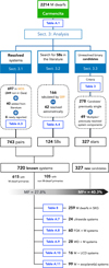 |
Fig. 2 Schematic summary of our analysis (Section 3). |
| In the text | |
|
Fig. 3 Comparison of projected separations tabulated by the WDS and measured by us using Gaia astrometry. The solid and dashed grey lines represent the 1:1 relation, and the differences in 10%, respectively. The magenta circles are stars beyond this limit. The error bars are rather small for almost all cases due to the high precision of Gaia’s astrometry and they have therefore been omitted. |
| In the text | |
|
Fig. 4 Comparative analysis of the proper motions and distances of the identified pairs. Top: ∆PA vs µ ratio diagram, where the dashed grey lines set the upper limits of our criteria for physical association (Eqs. (2) and (3)). The red open circles are pairs that do not comply, or do so partially, with those criteria, respectively. Bottom: comparison of distances of the companions (denoted ‘B+’) and their corresponding primaries (‘A’). The amber circles are pairs that do not comply with our criterion (Eq. (1)). Our Carmencita M dwarf may be the primary (i.e. the most massive) or a companion in the system. |
| In the text | |
|
Fig. 5 RUWE as a function of G magnitude for single stars (pink open circles) and stars in multiple systems (open blue circles). The histograms follow the same colour coding. RUWE = 2.0 (thick red dashed line), used in this work, leaves behind ∼80% of the sample and is more conservative than the traditionally used RUWE = 1.4 (thin black dashed line). |
| In the text | |
|
Fig. 6 Gaia DR3 statistical indicators of very close multiplicity. Top : astrometric_excess_noise (ϵ) vs RUWE. Middle : σ(Vr) vs G. Bottom: ipd_gof_harmonic_amplitude vs RUWE. In all panels, pink and blue open circles are for stars that were considered single and part of multiple systems, respectively, and the red thick dashed lines indicate the corresponding close binary selection criterion in Table 3. |
| In the text | |
|
Fig. 7 Light curves corresponding to the Gaia passbands GRP (red), G (green), and GBP (blue) for three cases: a single star (left), a known close (ρ = 0.1–0.2 arcsec) binary system (JNN 266, Janson et al. 2014b; middle), and a newly reported close (ρ ≈ 0.48 arcsec) binary system (right). Isolated outliers (represented by crosses) are photometric errors, not consistent with flares, automatically rejected by variability processing. The remaining light curves for the unresolved binary candidates with double-sequence patterns are displayed in Fig. A.1. |
| In the text | |
|
Fig. 8 Comparison of the standard deviations of GBP against that of G for single stars (light blue), stars in multiple systems (blue), and new unresolved binary candidates (red). The dashed line represent a 1:1 relation. The similar plot for GRP is omitted for simplicity. |
| In the text | |
|
Fig. 9 Stellar radius (ℛ, left) and mass (ℳ, right) as a function of the absolute magnitude (MG) valid in the M-dwarf domain. The red line represents the polynomial fit described in Table 4, and the red shaded area indicates the 1-σ level of uncertainty. |
| In the text | |
|
Fig. 10 Nomenclature of multiple systems based on the resolution of Gaia DR3 (blue circles) and 2MASS (orange circles). From left to right: ‘A+B’ (resolved in both surveys), ‘AB’ (only resolved in Gaia), ‘(AB)’ (not resolved either in Gaia or 2MASS, but resolved by adaptive optics, lucky imaging, or space imaging), and ‘Aab’ (spectroscopic binaries). Multiple systems can often be a combination of these cases. |
| In the text | |
|
Fig. 11 Absolute magnitude MG against GBP − GRP colour for all the stars in our sample and their resolved companions with full photometry available in Gaia DR3. Red crosses correspond to components of multiple systems that are very close, very faint, or both, resulting in compromised photometry. Very bright stars (e.g. Capella or Castor) are necessarily excluded for lacking Gaia photometric measurements. Very compact systems, not resolved by Gaia (Sect. 3.2), and resolved young stars (Sect. 4.5) lie above the main sequence. |
| In the text | |
|
Fig. 12 Schematic of the capabilities to identify binaries of the surveys and techniques exploited in this work (top) and difference in G magnitude as a function of angular separation for pairs that Gaia resolves (“AB” or “A+B”) and those for which WDS tabulated magnitude difference (bottom). Both figures follow the same scheme of colours. The nomenclature assigned to each scenario (see again Fig. 10) is also displayed. |
| In the text | |
|
Fig. 13 Physical separation as a function of the distance for all the pairs in our sample. The grey dashed lines represent projected angular separations, ρ = s/d, in dex. |
| In the text | |
|
Fig. 14 Cumulative (top) and non-cumulative (bottom) distribution of physical separations for all the pairs in our sample. The white dashed lines in the upper panel are power-law fits for the ranges 7–80 au and 80–3000 au, respectively. The grey vertical dashed lines delimit these ranges. |
| In the text | |
|
Fig. 15 Physical separation (top) and binding energy (bottom) as a function of system total mass. In the bottom panel, sizes are proportional to the physical separation from the primary. Red open circles highlight in both panels the most fragile pairs ( |
| In the text | |
|
Fig. 16 Mass ratios as a function of primary star mass (top) and projected physical separation (bottom), only for M-dwarf primaries. The red dashed line marks q = 1. The gradient map in the background represents the spectral types from M0.0 V to M9.0 V (Cifuentes et al. 2020) following the same scheme as in Fig. 1. |
| In the text | |
Current usage metrics show cumulative count of Article Views (full-text article views including HTML views, PDF and ePub downloads, according to the available data) and Abstracts Views on Vision4Press platform.
Data correspond to usage on the plateform after 2015. The current usage metrics is available 48-96 hours after online publication and is updated daily on week days.
Initial download of the metrics may take a while.