| Issue |
A&A
Volume 675, July 2023
BeyondPlanck: end-to-end Bayesian analysis of Planck LFI
|
|
|---|---|---|
| Article Number | A10 | |
| Number of page(s) | 32 | |
| Section | Cosmology (including clusters of galaxies) | |
| DOI | https://doi.org/10.1051/0004-6361/202244819 | |
| Published online | 28 June 2023 | |
BEYONDPLANCK
X. Planck Low Frequency Instrument frequency maps with sample-based error propagation
1
Institute of Theoretical Astrophysics, University of Oslo, PO Box 1029, Blindern, 0315 Oslo, Norway
e-mail: This email address is being protected from spambots. You need JavaScript enabled to view it.
2
Department of Physics, Gustaf Hällströmin katu 2, University of Helsinki, Helsinki, Finland
3
Helsinki Institute of Physics, Gustaf Hällströmin katu 2, University of Helsinki, Helsinki, Finland
4
Dipartimento di Fisica, Università degli Studi di Milano, Via Celoria, 16, Milano, Italy
5
INAF-IASF Milano, Via E. Bassini 15, Milano, Italy
6
INFN, Sezione di Milano, Via Celoria 16, Milano, Italy
7
INAF-Osservatorio Astronomico di Trieste, Via G.B. Tiepolo 11, Trieste, Italy
8
Planetek Hellas, Leoforos Kifisias 44, Marousi, 151 25
Greece
9
Department of Astrophysical Sciences, Princeton University, Princeton, NJ, 08544
USA
10
Jet Propulsion Laboratory, California Institute of Technology, 4800 Oak Grove Drive, Pasadena, CA, 91109
USA
11
Computational Cosmology Center, Lawrence Berkeley National Laboratory, Berkeley, CA, 94720
USA
12
Haverford College Astronomy Department, 370 Lancaster Avenue, Haverford, PA, 19041
USA
13
Max-Planck-Institut für Astrophysik, Karl-Schwarzschild-Str. 1, 85741 Garching, Germany
14
Dipartimento di Fisica, Università degli Studi di Trieste, Via A. Valerio 2, Trieste, Italy
Received:
25
August
2022
Accepted:
16
November
2022
Abstract
We present Planck Low Frequency Instrument (LFI) frequency sky maps derived within the BEYONDPLANCK framework. This framework draws samples from a global posterior distribution that includes instrumental, astrophysical, and cosmological parameters, and the main product is an entire ensemble of frequency sky map samples, each of which corresponds to one possible realization of the various modeled instrumental systematic corrections, including correlated noise, time-variable gain, as well as far sidelobe and bandpass corrections. This ensemble allows for computationally convenient end-to-end propagation of low-level instrumental uncertainties into higher-level science products, including astrophysical component maps, angular power spectra, and cosmological parameters. We show that the two dominant sources of LFI instrumental systematic uncertainties are correlated noise and gain fluctuations, and the products presented here support – for the first time – full Bayesian error propagation for these effects at full angular resolution. We compared our posterior mean maps with traditional frequency maps delivered by the Planck Collaboration, and find generally good agreement. The most important quality improvement is due to significantly lower calibration uncertainties in the new processing, as we find a fractional absolute calibration uncertainty at 70 GHz of Δg0/g0 = 5 × 10⁻⁵, which is nominally 40 times smaller than that reported by Planck 2018. However, we also note that the original Planck 2018 estimate has a nontrivial statistical interpretation, and this further illustrates the advantage of the new framework in terms of producing self-consistent and well-defined error estimates of all involved quantities without the need of ad hoc uncertainty contributions. We describe how low-resolution data products, including dense pixel-pixel covariance matrices, may be produced from the posterior samples directly, without the need for computationally expensive analytic calculations or simulations. We conclude that posterior-based frequency map sampling provides unique capabilities in terms of low-level systematics modeling and error propagation, and may play an important role for future Cosmic Microwave Background (CMB) B-mode experiments aiming at nanokelvin precision.
Key words: ISM: general / cosmology: observations / diffuse radiation / Galaxy: general / cosmic background radiation
© The Authors 2023
 Open Access article, published by EDP Sciences, under the terms of the Creative Commons Attribution License (https://creativecommons.org/licenses/by/4.0), which permits unrestricted use, distribution, and reproduction in any medium, provided the original work is properly cited.
This article is published in open access under the Subscribe to Open model. This email address is being protected from spambots. You need JavaScript enabled to view it. to support open access publication.
1. Introduction
The current state of the art in all-sky cosmic microwave background (CMB) observations is provided by the Planck satellite (Planck Collaboration I 2020), which observed the microwave sky in nine frequency bands (30–857 GHz) between 2009 and 2013. This experiment followed in the footsteps of Cosmic Background Explorer (COBE, Mather 1982) and Wilkinson Microwave Anisotropy Probe (WMAP, Bennett et al. 2003), improving frequency coverage, sensitivity, and angular resolution, and ultimately resulted in constraints on the primary CMB temperature fluctuations that are limited by cosmic variance, rather than instrumental noise or systematics.
The Planck consortium produced three major data releases, labeled 2013, 2015, and 2018 (Planck Collaboration II 2014, 2016, 2020), respectively, each improving the quality of the basic frequency maps in terms of the overall signal-to-noise ratio and systematics control. Several initiatives to further improve the quality of the Planck maps also began after the Planck 2018 legacy release, as summarized by SRoll2 (Delouis et al. 2019), Planck PR4 (sometimes also called NPIPE; Planck Collaboration Int. LVII 2020), and BEYONDPLANCK (BeyondPlanck Collaboration 2023).
The BEYONDPLANCK project builds directly on experiences gained during the last years of the Planck analysis, and focuses in particular on the close relationship between the various steps involved in the data analysis, including low-level time-ordered data processing, mapmaking, high-level component separation, and cosmological parameter estimation. As described in BeyondPlanck Collaboration (2023), the main goal of BEYONDPLANCK is to implement and deploy a single statistically coherent analysis pipeline to the Planck Low-Frequency Instrument (LFI; Planck Collaboration II 2020), processing raw uncalibrated time-ordered data into final astrophysical component maps and angular CMB power spectra within one single code, without the need for intermediate human intervention. This is achieved by implementing a Bayesian end-to-end analysis pipeline, which for convenience is integrated in terms of a software package called Commander3 (Galloway et al. 2023a). The current paper focuses on the 30, 44, and 70 GHz LFI frequency maps, and compares these novel maps with previous versions, both from Planck 2018 and PR4.
Map-making in a CMB analysis chain compresses time-ordered data (TOD) into sky maps. These TOD contain contributions from many instrumental effects, and those strongly affect the statistical properties of the resulting maps. For LFI, instrumental effects have traditionally been modeled in terms of three main components, namely white (uncorrelated) thermal noise, 1/f (correlated) noise, and general systematics (Mennella et al. 2010; Zacchei et al. 2011). The white noise is, by definition, uncorrelated between pixels, and its statistical properties are therefore straightforward to characterize and propagate to higher-level science products. In contrast, the correlated 1/f noise component manifests itself as extended stripes in maps, which significantly correlate pixels along the scanning path of the main beam. The same also holds true for general classes of systematic effects, including, for instance, gain fluctuations or bandpass mismatch between detectors. The goal of mapmaking is to suppress these effects as much as possible, while ideally leaving the astrophysical signal and white noise unchanged.
Traditionally, the actual mapmaking step in CMB analysis pipelines has primarily focused on the correlated noise component (e.g., Tegmark et al. 1997; Ashdown et al. 2007, and references therein), while general systematics corrections have been applied in a series of preprocessing steps. One particularly flexible method that has emerged during this work is the so-called destriping (Delabrouille 1998; Burigana et al. 1999; Maino et al. 1999, 2002; Keihänen et al. 2004, 2005, 2010; Kurki-Suonio et al. 2009), in which the 1/f noise component is modeled by a sequence of constant offsets, often called baselines. Furthermore, in generalized destriping, as for instance implemented in the Madam code (Keihänen et al. 2005, 2010), prior knowledge of noise properties can be utilized to better constrain the baseline amplitudes, at which point the optimal maximum-likelihood solution may be derived as a limiting case.
Toward the end of the Planck analysis period, however, a major effort was undertaken to include the treatment of some instrumental systematic effects (other than 1/f noise) directly into the pipeline, and several codes that simultaneously account for mapmaking, systematic error mitigation and component separation were developed. In particular, these integrated approaches were pioneered by SRoll (Planck Collaboration III 2020) and Planck PR4 (Planck Collaboration Int. LVII 2020), both of which adopted a template-based linear regression algorithm to solve the joint problem.
In contrast, the BEYONDPLANCK framework described in BeyondPlanck Collaboration (2023) and its companion papers adopts a more general approach, in which a full joint posterior distribution is sampled using standard Markov chain Monte Carlo methods. In this framework, the correlated noise is simply sampled as one of many components, together with corrections for gain fluctuations, bandpass mismatch, etc., and for each iteration in the Markov chain a new frequency map is derived. This ensemble of frequency maps then serves as a highly compressed representation of the full posterior distribution that can be analyzed in a broad range of higher-level analyses. Indeed, this approach implements for the first time a true Bayesian end-to-end error propagation for high-resolution CMB experiments, from raw uncalibrated time-ordered data to final cosmological parameter estimates.
The rest of the paper is organized as follows. In Sect. 2 we give an introduction to and overview of the BEYONDPLANCK analysis framework, focusing on the aspects that are most relevant for mapmaking and systematic error propagation. In Sect. 3 we inspect the Markov chains that result from the posterior sampling process, and quantify correlations at the frequency map level. Next, in Sect. 4 we present the resulting BEYONDPLANCK posterior mean frequency maps, and in Sect. 5 we compare these with previous Planck analyses. In Sect. 6 we consider end-to-end error propagation, both in the form of individual posterior samples and conventional covariance matrices, and in Sect. 7 we summarize the various systematic error corrections that are applied to each frequency map. Finally, we conclude in Sect. 8.
2. BEYONDPLANCK mapmaking and end-to-end error propagation
2.1. Statistical framework
The BEYONDPLANCK framework may be succinctly summarized in terms of a single parametric model that includes both astrophysical and instrumental components. The motivation and derivation of the specific BEYONDPLANCK data model is described in BeyondPlanck Collaboration (2023), and takes the following form,
![Mathematical equation: $$ \begin{aligned}&d_{j,t} = g_{j,t}\mathsf P _{tp,j}\left[\mathsf B ^{\mathrm{symm} }_{pp^{\prime },j}\sum _{c} \mathsf M _{cj}(\beta _{p^{\prime }}, \Delta _{\mathrm{bp}}^{j})a^c_{p^{\prime }} + \mathsf B ^{\mathrm{asymm} }_{j,t}\left(\boldsymbol{s}^{\mathrm{orb} }_{j} + \boldsymbol{s}^{\mathrm{fsl} }_{t}\right)\right] + \nonumber \\&\qquad + s^\mathrm{1\,Hz }_{j,t} + n^{\mathrm{corr} }_{j,t} + n^{\mathrm{w} }_{j,t}, \end{aligned} $$](/articles/aa/full_html/2023/07/aa44819-22/aa44819-22-eq1.gif) (1)
(1)
where j is a radiometer label, t is a time sample, p is a pixel on the sky, and c is an astrophysical component. Further, dj, t is the measured data; gj, t is the instrumental gain; Ptp, j is the NTOD × 3Npix pointing matrix; Bj denotes the beam convolution; Mcj(βp, Δbp) is an element of a foreground mixing matrix that depends on both a set of nonlinear spectral energy density parameters, β, and instrumental bandpass parameters, Δbp;  is the amplitude of a sky signal component;
  is the orbital CMB dipole signal;
  is a contribution from far sidelobes;
  represents an electronic 1 Hz spike correction;
  is correlated instrumental noise; and
  is uncorrelated (white) instrumental noise, which is assumed to be Gaussian distributed with covariance Nwn.
To build intuition regarding the various terms involved in Eq. (1), Fig. 1 shows an arbitrarily selected 3-minute segment of the various TOD components for one LFI radiometer. The top panel shows the raw radiometer measurements, d, while the second panel shows the sky model contribution described by the first term on the right-hand side in Eq. (1) for signal parameters corresponding to one randomly selected sample. The slow oscillations in this function represent the CMB (Solar and orbital) dipole, while the sharp spikes correspond to the bright Galactic plane signal. The small fluctuations super-imposed on the slow CMB dipole signal are dominated by CMB fluctuations, and measuring these is the single most important goal of any CMB experiment. The third panel shows the correlated noise, ncorr, which is stochastic in nature, but exhibits long-term temporal correlations. The fourth panel shows the orbital CMB dipole, sorb, which represents our best-known calibration source. However, it only has a peak-to-peak amplitude of about 0.5 mK, and is as such nontrivial to measure to high precision in the presence of the substantial correlated noise and other sky signals seen above. The fifth panel shows the far sidelobe response, which is generated by convolving the sky model with the 4π instrument beam after nulling a small area around the main beam. The last term in Eq. (1) is the contribution from electronic 1 Hz spikes, s1 Hz, and is shown in the sixth panel. The seventh panel shows a correction term for so-called bandpass and beam leakages, sleak, which accounts for differing response functions among the radiometers used to build a single frequency map. This is not a stochastic term in its own right, but rather given deterministically by the combination of the sky model and the instrument bandpasses and beams. The bottom panel shows the difference between the raw data and all the individual contributions, which ideally should be dominated by white noise. Intuitively, the BEYONDPLANCK pipeline simply aims to estimate the terms shown in the second to sixth panels in this figure from the top panel.
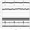 |
Fig. 1. Time-ordered data segment for the 30 GHz LFI 27M radiometer. From top to bottom, the panels show 1) raw calibrated TOD, d/g; 2) sky signal, ssky; 3) calibrated correlated noise, ncorr/g; 4) orbital CMB dipole signal, sorb; 5) sidelobe correction, ssl; 6) electronic 1 Hz spike correction, s1 Hz; 7) leakage mismatch correction, sleak; and 8) residual TOD, dres = (d − ncorr − s1 Hz)/g − ssky − sorb − sleak − ssl. |
For notational simplicity, we define ω ≡ {a, β, g, Δbp, ncorr, …} to be the set of all free parameters in Eq. (1), and we fit this to d by mapping out the posterior distribution, P(ω ∣ d). According to Bayes’ theorem, this distribution may be written
 (2)
(2)
where ℒ(ω)≡P(d ∣ ω) is the likelihood, and P(ω) is some set of priors. The likelihood may be written out explicitly by first defining stot(ω) to be the full expression on the right-hand side of Eq. (1), except the white noise term, and then noting that d − stot = nwn, and therefore
 (3)
(3)
The priors are less well defined, and for an overview of both informative and algorithmic priors used in the current analysis, see BeyondPlanck Collaboration (2023).
It is important to note that P(ω ∣ d) involves billions of free parameters, all of which are coupled into one highly correlated and non-Gaussian distribution. As such, mapping out this distribution is computationally nontrivial. Fortunately, the statistical method of Gibbs sampling (Geman & Geman 1984) allows users to draw samples from complex joint distribution by iteratively sampling from each conditional distribution. Using this method for global CMB analysis was first proposed by Jewell et al. (2004) and Wandelt et al. (2004), nearly two decades ago. And has finally been applied here for the first time to real data. As described in BeyondPlanck Collaboration (2023), we write the BEYONDPLANCK Gibbs chain schematically as
 (4)
(4)
 (5)
(5)
 (6)
(6)
 (7)
(7)
 (8)
(8)
 (9)
(9)
 (10)
(10)
 (11)
(11)
where symbol ← has the meaning that we set variable on the left-hand side equal to the sample from the distribution on the right-hand side.
2.2. Mapmaking
In the BEYONDPLANCK framework, frequency maps are not independent stochastic variables in their own right, but they serve rather as a deterministic compression of the full dataset from TOD into sky pixels, conditioning on other actual stochastic parameters, such as g and ncorr. To derive these compressed frequency maps, we first compute the residual calibrated TOD for each detector,
 (12)
(12)
where
 (13)
(13)
is the difference between the sky signal as seen by detector j and the mean over all detectors; this term suppresses so-called bandpass and beam leakage effects in the final map (Svalheim et al. 2023). To the extent that the data model is accurate, rj, t contains only stationary sky signal and white noise, given the current estimates of other parameters in the data model. A proper frequency map may therefore be obtained simply by binning r into a map, that is, by solving the following equation for each pixel,
 (14)
(14)
It is important to note that the residual in Eq. (12) depends explicitly on ω, and different combinations of g, ncorr, etc., will result in a different sky map. As such, a frequency map in the BEYONDPLANCK framework represents just one possible realization, and in each iteration in the Markov chain a new frequency map is derived. The final result is an entire ensemble of frequency maps,  , each with different combinations of systematic effects. The mean of these samples may be compared to traditional maximum-likelihood estimates, as indeed is done in Sect. 5, but it is important to emphasize that the main product from the current analysis is the entire ensemble of sky maps, not the posterior mean. The reason is that only by considering the full set of individual samples is it possible to fully propagate uncertainties into high-level results.
It is also important to note that this ensemble by itself does not propagate white noise uncertainties, as the residual in Eq. (12) only subtracts instrumental systematic effects. This is a purely implementational choice, and we could in principle also have added a white noise fluctuation to each realization. However, because the white noise is uncorrelated both in time and between pixels, its 3 × 3 Stokes {T, Q, U} covariance is very conveniently described in terms of the coupling matrix in Eq. (14), and reads
 (15)
(15)
![Mathematical equation: $$ \begin{aligned}&\quad = \left[\begin{array}{ccc} \sum \frac{1}{\sigma _{0,j}^2}&\sum \frac{\cos 2\psi _{j,t}}{\sigma _{0,j}^2}&\sum \frac{\sin 2\psi _{j,t}}{\sigma _{0,j}^2} \\ \sum \frac{\cos 2\psi _{j,t}}{\sigma _{0,j}^2}&\sum \frac{\cos ^2 2\psi _{j,t}}{\sigma _{0,j}^2}&\sum \frac{\cos 2\psi _{j,t} \sin 2\psi _{j,t}}{\sigma _{0,j}^2} \\ \sum \frac{\sin 2\psi _{j,t}}{\sigma _{0,j}^2}&\sum \frac{\sin 2\psi _{j,t} \cos 2\psi _{j,t}}{\sigma _{0,j}^2}&\sum \frac{\sin ^2 2\psi _{j,t}}{\sigma _{0,j}^2} \end{array}\right]^{-1}, \end{aligned} $$](/articles/aa/full_html/2023/07/aa44819-22/aa44819-22-eq23.gif) (16)
(16)
where σ0, j and ψj, t denote the time-domain white noise rms per sample and the polarization angle for detector j and sample t, and the sums run over all samples. This may be evaluated and stored compactly pixel-by-pixel, and it allows for computational efficient and analytical white noise-only error propagation in higher level analyses. In addition, we note that most external and already existing CMB analysis tools already expect a mean map and white noise covariances as inputs, and this uncertainty description is particularly convenient for those1.
2.3. Resource requirements
In this analysis, we consider only the Planck LFI data, for which the raw data volume is about 8 TB as provided directly by the LFI DPC. However, using Huffman compression, and removing noncritical housekeeping information, this may be reduced to 861 GB through Huffman compression. Also accounting for non-TOD objects, the total data volume required for this full multiband analysis is 1.5 TB, as further detailed by Galloway et al. (2023a).
The processing time required for initialization is 64 CPU-hrs, whereas each Gibbs sample takes 164 CPU-hrs, making the initialization step comparetively small to the sampling step. The majority of the sampling time (97 CPU-hrs) is spent on low-level TOD processing, and this includes Huffman decompression (10 CPU-hrs), sidelobe evaluation (10 CPU-hrs), gain sampling (6 CPU-hrs), correlated noise sampling (30 CPU-hrs), etc. The rest of the Gibbs loop time is dominated by component separation tasks, most notably signal amplitude sampling (24 CPU-hrs) and spectral parameter (40 CPU-hrs) sampling.
A total of 4000 Gibbs samples are produced in the current processing, and the total cost for the full analysis is thus about 650 000 CPU-hrs. It is important to note that this cost accounts both for model fitting and error estimation, and there is no need for separate analysis of Monte Carlo simulations (Brilenkov et al. 2023), except for algorithm validation. Noting that the overall computational cost of this algorithm scales roughly linear with data volume (because of TOD segmenting), these numbers may be used to derive a very rough rule of thumb for the total cost estimate: Analyzing 1 TB of raw uncompressed data costs 𝒪(105) CPU-hrs.
3. Markov chains and correlations
The algorithm outlined in Eqs. (4)–(11) is a Markov chain, and must as such be initialized. To reduce the overall burn-in time and minimize the risk of being trapped in a local nonphysical likelihood minimum, we perform this operation in stages. Specifically, we first initialize the instrumental parameters on the best-fit values reported by the official Planck LFI Data Processing Center (DPC) analysis (Planck Collaboration II 2020), and we fix the sky model at the Planck 2015 Astrophysical Sky Model (Planck Collaboration X 2016). (The Planck 2018 release did not include separate low-frequency components – synchrotron, free-free, and AME – which are essential for the current analysis). Then each frequency channel is optimized separately, without feedback to the sky model. Once a reasonable fit is obtained for each channel, the model is loosened up, and a new analysis is started that permits full feedback between all parameters. In practice, multiple runs are required to resolve various issues, whether they are bug fixes or model adjustments, and in each case we restart the run at the most advanced previous chain, to avoid repeating the burn-in process, which can take many weeks. The final results presented in the current data release correspond to the tenth such analysis iteration, and the parameter files and products (Galloway et al. 2023a) are labeled by “BP10”. We strongly recommend future analyses aiming to add additional datasets to the current model to follow a similar analysis path, fixing the sky model on the current BEYONDPLANCK chains, and in the beginning only optimize instrumental parameters per new frequency channel. This is likely to vastly reduce both the debug and burn-in time, as it prevents the chains from exploring obviously nonphysical regions of the parameter space.
The final BP10 results consist of four independent Markov chains, each with a total of 1000 Gibbs samples. We conservatively removed 200 samples from each chain as burn-in (Paradiso et al. 2023), but it is important to note that we have not seen statistically compelling evidence for significant chain nonstationarity after the first few tens of samples. A total of 3200 samples has been retained for full analysis.
Figure 2 shows a small subset of these samples for various parameters that are relevant for the LFI frequency maps. The two colors indicate two different Markov chains. From top to bottom, in the left column the plotted parameters are Stokes I, Q, and U parameters for each of the 30, 44, and 70 GHz frequency maps for two low-resolutions Nside = 16 pixels, namely pixels 340 (which is located in a low-foreground region of the northern high-latitude sky) and 1960 (which is located in a high-foreground region south of the Galactic center). Similarly, the right column show synchrotron, free-free, thermal dust, and CMB amplitudes, as well the bandpass correction and the correlated noise parameters for one pointing period (PID) for the 30 GHz 27M radiometer. Overall, we see that the frequency map pixel values have a relatively short correlation length, and the chains mix well and appear statistically stationary. In general, the correlation lengths appear much longer for the instrumental parameters and some of the astrophysical parameters, in particular the synchrotron intensity amplitude. This makes intuitively sense, as we see from the definition of the TOD residual in Eq. (12) that the frequency maps depend only weakly on the sky model through the far sidelobe and leakage corrections, both of which are small in terms of absolute amplitudes (see Fig. 1), and at second order through the gain, which uses the sky model for calibration purposes.
 |
Fig. 2. Trace plots of a set of selected frequency map parameters and related quantities; see main text for full definitions. The different colors indicate two independent Gibbs chains, and the 340 and 1960 subscripts indicate HEALPix pixel numbers at resolution Nside = 16 in ring ordering. |
This observation is important when comparing frequency maps generated through Bayesian end-to-end processing with those generated through traditional frequentist methods; although the Bayesian maps are formally statistically coupled through the common sky model, these couplings are indeed weak, and their correlations are fully quantified through the sample ensemble. It is also important to note that precisely the same type of couplings exist in the traditional maps, as they also depend on a sky model to estimate the gain and perform sidelobe and bandpass corrections in precisely the same manner as the current algorithm. The only fundamental difference is that the traditional methods usually only adopt one fixed sky model for these operations (e.g., Planck Collaboration II 2020; Planck Collaboration III 2020), and therefore do not propagate its uncertainties, while the Bayesian approach considers an entire ensemble of different sky models, and thereby fully propagates astrophysical uncertainties.
In Fig. 3 we plot the Pearson’s correlation coefficient between any two pairs of parameters shown in Fig. 2. The upper triangle shows full correlations computed directly from the raw Markov chains, while the bottom triangle shows the same after high-pass filtering each chain with a boxcar filter with a 5-sample window; the latter is useful to highlight correlations within the local white noise distribution (i.e., fast variations in Fig. 2), while the former accounts also for strong long-distance degeneracies (i.e., slow drifts in Fig. 2). Monopoles have been removed from the intensity frequency maps, except in the last row of Fig. 3, which shows correlations that also including monopole variations.
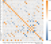 |
Fig. 3. Correlation coefficients between the same parameters as shown in Fig. 2. The subscripts a and b relate to the 340 and 1960 HEALPix pixel numbers. The lower triangle shows raw correlations, while the upper triangle shows correlations after high-pass filtering with a running mean with a 10-sample window. For further explanation of and motivation for this filtering, see Andersen et al. (2023). |
Going through these in order of strength, we start with the correlated noise parameters. As described by Ihle et al. (2023), the current processing assumes a standard 1/f noise power spectral density,  , for the 70 GHz channel, which is extended with a log-normal term for the 30 and 44 GHz channels to account for a previously undetected power excess between 0.1–1 Hz. This additional term introduces a strong degeneracy with α and fknee at the 0.8–0.9 level after high-pass filtering. However, the actual frequency map only depends on the sum of these components, and internal noise PSD degeneracies are completely irrelevant for the final sky maps. This is seen by the fact that the correlation coefficient between any noise parameter and the sky map pixels is at most 0.06.
The second strongest correlations are seen in the bottom row, which shows the 30 GHz intensity in pixel a correlated with all other quantities. Here we see that pixels a and b are 97% correlated internally in the 30 GHz channel map, and pixel a is also 84% (42%) correlated with the same pixel in the 44 GHz (70 GHz) channel. These strong correlations are due to the fact that the BEYONDPLANCK maps have monopoles determined directly from the astrophysical foreground model, and all frequency maps therefore respond coherently to changes in, say, the free-free offset. After removing this strong common mode the correlations among the frequency maps fall to well below 10%, as seen in the top section of the plot.
Thirdly, we see that there are strong correlations among the sky model parameters (CMB, synchrotron, free-free, and thermal dust emission), typically at the 0.3–0.6 level, and some of these also extend to the actual frequency maps. Starting with the internal sky model degeneracies, strong correlations between synchrotron, free-free, and AME are fully expected due to their similar SEDs and the limited dataset used in the current analysis. Qualitatively similar results were reported by Planck Collaboration X (2016) and Planck Collaboration XXV (2016) even when including the intermediate HFI frequencies, and excluding the HFI data obviously does nothing to reduce these correlations. The large correlations with respect to the frequency maps are perhaps more surprising, given the statements above that the frequency maps only depend very weakly on the sky model parameters. However, it is important to note that the converse does not hold true; the sky model depends strongly on the frequency maps, and these dependencies are encoded in Fig. 3. Two concrete examples are CMB polarization, which is most tightly correlated with the 70 GHz channel, and the synchrotron polarization amplitude, which is most tightly correlated with the 30 GHz channel.
The fourth most notable correlation is seen among the three Stokes parameters for a single pixel, and in particular between Q and U for which the intrinsic sky signal level is small, and these effects are therefore relatively more important. Even though white noise does not contribute to these Markov chains, the correlated noise and systematic effects also behave qualitatively similar as white noise with respect to the Planck scanning strategy.
4. BEYONDPLANCK frequency maps
4.1. General characteristics
We now turn our attention to the coadded frequency maps, and compare the BEYONDPLANCK maps with the corresponding Planck 2018 maps in terms of various key quantities in Table 1. Unless noted otherwise, Planck values are reproduced directly from Planck Collaboration II (2020). Entries marked with three dots indicate that the BEYONDPLANCK values are identical to the Planck values, while dashed entries for Planck indicate that those values are undefined.
Frequency map comparison between Planck 2018 and BEYONDPLANCK products.
Starting from the top, we see that the BEYONDPLANCK maps adopt a HEALPix2 (Górski et al. 2005) resolution of Nside = 512 for the 30 and 44 GHz channels and Nside = 1024 for the 70 GHz, while the Planck maps use Nside = 1024 for all three channels. In this respect, it is worth noting that the beam width of the three channels are 30′, 27′, and 14′ (Planck Collaboration II 2020), respectively, while the HEALPix pixel size is 7′ at Nside = 512 and 3.4′ at Nside = 1024. A useful rule of thumb for the HEALPix grid is that maps should have at least 2.5–3 pixels per beam FWHM to be proper bandwidth limited at ℓmax ≈ 2.5 Nside, above which HEALPix spherical harmonic transforms gradually become more nonorthogonal (Górski et al. 2005). With 3.9 pixels per beam FWHM, this rule is more than satisfied at Nside = 512 for the 30 and 44 GHz beams, while it would not be satisfied at 70 GHz, with only two pixels per beam FWHM. As essentially all modern component separation and CMB power spectrum methods today are anyway required to operate with multiresolution data, simply to combine data from LFI, HFI and WMAP, there is little compelling justification for maintaining identical pixel resolution among the three LFI channels, and we instead choose to optimize CPU and memory requirements for the 30 and 44 GHz channels.
The second entry in Table 1 lists the nominal center frequency of each band. As discussed by Svalheim et al. (2023), the BEYONDPLANCK model includes the 30 GHz center frequency as a free parameter, but fixes the 44 and 70 GHz center frequencies at their default values. The overall shift for the 30 GHz channel is 0.2 GHz, with corresponding implications in terms of unit conversions, color corrections, and bandpass integration. In addition to this 30 GHz correction, the BEYONDPLANCK processing also includes entirely reprocessed bandpasses for all detectors, mitigating artifacts from standing waves which affected bandpass measurements in the prelaunch calibration campaign (Zonca et al. 2009; Svalheim et al. 2023), and we highly recommend using these improved bandpass profiles for any future processing of either the original Planck or the new BEYONDPLANCK LFI maps.
The four next entries in Table 1 list either “typical” (for Planck 2018; Planck Collaboration II 2020) or frequency- and time-averaged (for BEYONDPLANCK; Ihle et al. 2023) noise PSD parameters. Overall, these agree well between the two analyses. However, it is important to emphasize that whereas the Planck analysis assumes that the instrumental parameters listed in lines 3–6 of Table 1 to be constant throughout the full mission during mapmaking, the BEYONDPLANCK processing allows for hourly variations in all these parameters. The BEYONDPLANCK method leads as such both to more optimal noise weighting in the final map, and also to more accurate full-mission white noise estimates. We also see that the additional log-normal correlated noise contribution accounts for as much as 53% of the white noise level at intermediate frequencies in the 30 GHz channel, and 28% at 44 GHz (Ihle et al. 2023). This term is neither included in the Planck noise model nor simulations.
The next entry in Table 1 lists the total data volume that is actually coadded into the final maps, as measured in units of detector-hours. In general, the accepted BEYONDPLANCK data volume is about 9% larger than the Planck 2018 data volume, and this is because the current processing also includes the so-called “repointing” periods, which are short intervals of about 5–8 minutes between each Planck pointing period. These data were originally excluded by an abundance of caution from the official Planck processing because the pointing model could not be demonstrated to satisfy the arcsecond pointing requirements defined at the beginning of the mission. However, Planck Collaboration Int. LVII (2020) have subsequently demonstrated that these data perform fully equivalently in terms of null maps and power spectra as the regular mission data, and the potential additional arcsecond-level pointing uncertainties are negligible compared to the overall instrument noise level. We therefore follow Planck PR4, and include these observations.
The last entry in Table 1 compares the nominal absolute calibration uncertainties of Planck 2018 and BEYONDPLANCK (Svalheim et al. 2023), and this may very well quantify the single most important difference between the two sets of products. For the 70 GHz the nominal absolute BEYONDPLANCK calibration uncertainty is as much as 40 times smaller than the Planck 2018 uncertainty, corresponding to a fractional uncertainty of Δg0/g0 = 5 × 10⁻⁵. For the 30 GHz channel, the corresponding ratio is 24.
Clearly, when faced with such large uncertainty differences, two questions must be immediately addressed, namely, 1) “how reasonable the quoted uncertainties are”, and 2) if they are reasonable, “what the physical and algorithmic origin of these large differences is” Starting with the first question, it is useful to adopt the CMB Solar dipole amplitude as a reference. This amplitude depends directly, but by no means exclusively, on the 70 GHz absolute calibration; other important (and, in fact, larger) sources of dipole amplitude uncertainties include foreground and analysis mask marginalization and the uncertainty in the CMB monopole, TCMB = 2.7255 ± 0.0005 mK (Fixsen 2009; Colombo et al. 2023). For BEYONDPLANCK, the total CMB Solar dipole posterior standard deviation is 1.4 μK, while the conditional uncertainty predicted by the 70 GHz absolute calibration only is 3.36 mK × 5 × 10−5 = 0.2 μK, which is at least theoretically consistent with a total dipole uncertainty of 1.4 μK, given the other sources of uncertainty. For Planck 2018, the corresponding predicted conditional dipole uncertainty is 3.36 mK × 200 × 10−5 = 7 μK, which is more than twice as large as the corresponding full Solar dipole uncertainty. The quoted LFI absolute gain uncertainties thus appear to be overly conservative, and cannot be taken as a realistic absolute gain uncertainty at face value; the true uncertainty is most likely lower by at least a factor of two, and possibly as much as an order of magnitude.
Even after accounting for this factor, it is clear that the BEYONDPLANCK uncertainty is still significantly lower. To understand the origin of this difference, we recall the summary of the BEYONDPLANCK calibration approach provided by Gjerløw et al. (2023): Whereas Planck 2018 processes each frequency channel independently and assumes the large-scale CMB polarization signal to be zero during calibration, BEYONDPLANCK processes all channels jointly and uses external information from WMAP to constrain the large-scale CMB polarization modes that are poorly measured by Planck alone. Thus, the BEYONDPLANCK gain model contains fewer degrees of freedom than the corresponding Planck 2018 model, and it uses more data to constrain these degrees of freedom. The net result is a significantly more well-constrained calibration model.
4.2. Posterior mean maps and uncertainties
Figures 4–6 show the posterior mean Stokes T, Q, and U maps for each of the 30, 44, and 70 GHz channels. Note that the BEYONDPLANCK intensity sky maps retain the CMB Solar dipole. This is similar to Planck PR4 (Planck Collaboration Int. LVII 2020), but different from Planck 2018. For the remainder of the paper, we add the Planck 2018 Solar dipole back into the Planck 2018 frequency maps using the parameters listed by Planck Collaboration I (2020) when needed.
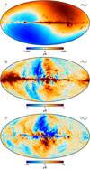 |
Fig. 4. Posterior mean maps for the 30 GHz frequency channel. From top to bottom: Stokes I, Q and U parameters. Maps have resolution Nside = 512, are presented in Galactic coordinates, and polarization maps have been smoothed to an effective angular resolution of 1° FWHM. |
 |
Fig. 5. Posterior mean maps for the 44 GHz frequency channel. From top to bottom: Stokes I, Q and U parameters. Maps have resolution Nside = 512, are presented in Galactic coordinates, and the polarization maps have been smoothed to an effective angular resolution of 1° FWHM. |
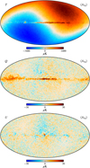 |
Fig. 6. Posterior mean maps for the 70 GHz frequency channel. From top to bottom: Stokes I, Q and U parameters. Maps have a HEALPix resolution of Nside = 1024, are presented in Galactic coordinates, and the polarization maps have been smoothed with a FWHM = 1° Gaussian beam. |
Figure 7 shows the posterior standard deviation evaluated pixel-by-pixel directly from the sample set, while Fig. 8 shows the diagonals of the white noise covariance matrices. The first point to notice is that the intensity scale of the white noise matrices is 75 μK, while the range for the posterior standard deviation is 2 μK. The Planck LFI maps are thus strongly dominated by white noise on a pixel level. However, the fundamental difference between these two sets of matrices is that while the white noise standard deviations scale proportionally with the HEALPix pixel resolution, Nside, the posterior standard deviation does not, and the spatial correlations in the latter therefore dominate on large angular scales.
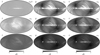 |
Fig. 7. Posterior standard deviation maps for each LFI frequency. Rows show, from top to bottom, the 30, 44 and 70 GHz frequency channels, while columns show, from left to right, the temperature and Stokes Q and U parameters. The 30 GHz standard deviation is divided by a factor of 3. Note that these maps do not include uncertainty from instrumental white noise, but only variations from the TOD-oriented parameters included in the data model in Eq. (1). |
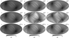 |
Fig. 8. White noise standard deviation maps for a single arbitrarily selected sample. Rows show, from top to bottom, the 30, 44 and 70 GHz frequency channels, while columns show, from left to right, the temperature and Stokes Q and U parameters. Note that the 70 GHz maps are scaled by a factor of 2, to account for the fact that this map is pixelized at Nside = 1024, while the two lower frequencies are pixelized at Nside = 512. |
A visually striking example of such spatial correlations is directly visible in the 30 GHz intensity panel in Fig. 7, which actually appears almost spatially homogeneous, and with an amplitude that is more than three times larger than the other channels. The reason for this homogeneous structure is that the per-pixel variance of the 30 GHz channel is strongly dominated by the same monopole variations seen in the bottom row of Fig. 3, and only small hints of the scanning pattern variations (from gain and correlated noise fluctuations) may be seen at high Galactic latitudes. Consequently, degrading the 30 GHz map to very low Nside’s will not change the per pixel posterior standard deviation at all, while the white noise level will eventually drop to sub-μK values.
Qualitatively speaking, similar considerations also hold for all the other effects seen in these plots, whether it is the synchrotron emission coupling seen in the 44 GHz intensity map, the Planck scanning induced gain and correlated noise features seen in the 30 and 44 GHz polarization maps, or the Galactic plane features seen in all panels. These are all spatially correlated, and do not average down with smaller Nside as expected for Gaussian random noise.
It is also interesting to note that the BEYONDPLANCK processing mask is clearly seen in the 44 GHz polarization standard deviations. This is because the TOD-level correlated noise within this mask is only estimated through a constrained Gaussian realization using high-latitude information and assuming stationarity (Ihle et al. 2023), and this is obviously less accurate than estimating the correlated noise directly from the measurements. Still, we see that this effect only increases the total marginal uncertainty by a modest 10–20%.
The motivation for introducing the processing mask during correlated noise and gain estimation is illustrated in Fig. 9, which shows the TOD-level residual,  , binned into sky maps. These plots summarize everything in the raw TOD that cannot be fitted by the model in Eq. (1). The clearly dominant features in these maps are Galactic plane residuals, which are due to a simplistic foreground model, and these are slightly modulated by the Planck scanning strategy through gain variations. At high Galactic latitudes, the dominant residuals are point sources and Gaussian noise. Regarding the point source residuals, we note that the current BEYONDPLANCK data model does not account for time variability (Rocha et al. 2023), and this should be added in a future extension. Without a processing mask, these residuals would bias the estimated gain and correlated noise model, and thereby also bias even the high-latitude sky. At the same time, it is important to note that the intensity scale in these plots is very modest, and by far most of the sky exhibits variations smaller than 3 μK.
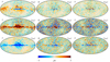 |
Fig. 9. Posterior mean total data-minus-model residual maps rν = dν − sν for BEYONDPLANCK LFI 30 (top), 44 (middle), and 70 GHz (bottom). All maps are smoothed to a common angular resolution of 2° FWHM. |
4.3. Peculiar artifacts removed by hand
Before ending this section, we note that a few scanning periods are removed by hand in the current analysis. These were identified by projecting the estimated correlated noise into sky maps, and an example of an older version of the 44 GHz ncorr map is shown in the top panel of Fig. 10. Overall, this map is dominated by coherent stripes, as expected for 1/f-type correlated noise, and there is also a negative imprint of the Galactic plane, which is typical of significant foreground residuals outside the processing mask. The latter effect was mitigated through better foreground modeling and a more conservative processing mask in the final production analysis. However, in addition to these well understood features, there are also two localized and distinct features in this plot. The first is a triangle, marked by PID 6144, and the second consists of two extended stripes marked by PID 14 416, both identified through a series of bi-section searches. The corresponding TOD residuals are shown in the bottom two panels; the black curve shows the raw residual, while the red curve shows the same after boxcar averaging with a 1-sec window. Here we see that the triangle feature comprises a series of 20 strong spikes separated by exactly one minute, which is identical to the Planck spin frequency, while the extended stripes are due to three slow oscillations.
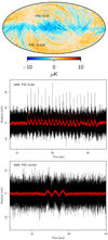 |
Fig. 10. Previously undetected TOD artifacts found by visual inspection of the (preliminary) correlated noise map for the 44 GHz channel shown in the top panel. The middle and lower panels show a zoom-in of the source PIDs, namely PID 6144 (for the “triangle feature”) and PID 14 416 (for the “dashed stripe feature”). In the two latter, the black curve shows the TOD residual, d − stot, for each sample, and the red curve shows the same after boxcar averaging with a 1 s window. |
An inspection of other detector residuals at the same time shows that the spike event is present in all 44 and 70 GHz detectors. Furthermore, a similar event is also present in PID 6126, and this is also spatially perfectly synchronized with the PID 6144 event, such that they appear superimposed in the top panel of Fig. 10. The effect is thus quite puzzling, as it appears naively to be stationary in the sky, and it was measured by all detectors for two separate 20-minute periods; but if it were a real signal, it would have to originate extremely close to the Planck satellite, since different detectors observe the signal in widely separated directions. It is difficult to imagine any true physical sources that could create such a signal, and we, therefore, conclude that it most likely is due to an instrumental glitch. At the same time, it is very difficult to explain why it appears as sky stationary at two different times. We do not have any plausible explanations for this signal, but it is obviously not a cosmological signal signal, and we, therefore, remove PIDs 6126 and 6144 by hand from the analysis.
In contrast, the PID 14 416 event takes the form of three slow oscillations and this looks very much like a thermal or electrical event on the satellite. We therefore also exclude this by hand. We note, however, that neither of these artifacts were detected during the nominal Planck analysis phase and this demonstrates the usefulness of the correlated noise and TOD residual maps in the current analysis as catch-all systematics monitors. Indeed, low-level analysis in the Bayesian framework may in fact be viewed as an iterative refinement process in which coherent signals in these maps are gradually removed through explicit parametric modeling, and assigned to well-understood physical effects. The fact that the correlated noise maps in Fig. 9 in Ihle et al. (2023) appear visually clean of significant artifacts provides some of the strongest evidence for low systematic contamination in the BEYONDPLANCK data products.
5. Comparison with Planck 2018 and PR4
Next, we compare the BEYONDPLANCK posterior mean LFI frequency maps with the corresponding Planck 2018 and PR4 products, and we start by showing difference maps in Fig. 11. All maps are smoothed to a common angular resolution of 2° FWHM, and a monopole has been subtracted from the intensity maps. To ensure that this comparison is well defined, the 2018 maps have been scaled by the uncorrected beam efficiencies (Planck Collaboration II 2020), and the best-fit Planck 2018 Solar CMB dipole has been added to each map, before computing the differences; both PR4 and BEYONDPLANCK maps are intrinsically beam efficiency corrected and they retain the Solar dipole.
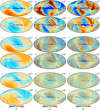 |
Fig. 11. Differences between BEYONDPLANCK and 2018 or PR4 frequency maps, smoothed to a common angular resolution of 2° FWHM. Columns show Stokes T, Q and U parameters, respectively, while rows show pair-wise differences with respect to the pipeline indicated in the panel labels. A constant offset has been removed from the temperature maps, while all other modes are retained. The 2018 maps have been scaled by their respective beam normalization prior to subtraction. |
Overall, we see that the BEYONDPLANCK maps agree with the other two pipelines to ≲10 μK in temperature, and to ≲4 μK in polarization. In temperature, we see that the dominant differences between Planck PR4 and BEYONDPLANCK are dipoles aligned with the Solar dipole, while differences with respect to the 2018 maps also exhibit a notable quadrupolar pattern. The sign of the PR4 dipole differences changes with frequency. This result is consistent with the original characterization of the PR4 maps derived through multifrequency component separation in Planck Collaboration Int. LVII (2020); that paper reports a relative calibration difference between the 44 and 70 GHz channel of 0.31%, which corresponds to 10 μK in the map domain. Overall, in temperature BEYONDPLANCK is thus morphologically similar to PR4, but it improves a previously reported relative calibration uncertainty between the various channels by performing joint analysis.
In polarization, the dominant large-scale structures appear to be spatially correlated with the Planck gain residual template presented by Planck Collaboration II (2020), and discussed by Gjerløw et al. (2023). These patterns are thus plausible associated with the large nominal calibration uncertainties between Planck 2018 and BEYONDPLANCK discussed in Sect. 4.1. It is additionally worth noting that the overall morphology of these difference maps is similar between frequencies, and that the amplitude of the differences falls with frequency. This strongly suggests that different foreground modeling plays a crucial role. In this respect, two observations are particularly noteworthy: First, while both the Planck 2018 and PR4 pipelines incorporate component separation as an external input as defined by the Planck 2015 data release (Planck Collaboration X 2016) in their calibration steps, BEYONDPLANCK performs a joint fit of both astrophysical foregrounds and instrumental parameters. Second, both the LFI DPC and the PR4 pipelines consider only Planck observations alone, while BEYONDPLANCK also exploits WMAP information to establish the sky model, which is particularly important to break scanning-induced degeneracies in polarization (Gjerløw et al. 2023).
We now turn our attention to the angular power spectrum properties of the BEYONDPLANCK frequency maps. Figure 12 shows auto-correlation spectra as computed with PolSpice (Chon et al. 2004) outside the Planck 2018 common component separation confidence mask (Planck Collaboration IV 2020), which accepts a sky fraction of 80%. All these spectra are clearly signal-dominated at large angular scales (as seen by the rapidly decreasing parts of the spectra at low ℓ’s), and noise-dominated at small angular scales (as seen by the flat parts of the spectra at high ℓ’s); note that the “signal” in these maps includes both CMB and astrophysical foregrounds. Overall, the three pipelines agree well at the level of precision supported by the logarithmic scale used here; the most striking differences appear to be variations in the high-ℓ plateau, suggesting notably different noise properties between the three different pipelines.
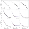 |
Fig. 12. Comparison between angular auto-spectra computed from the BEYONDPLANCK (black), Planck 2018 (blue), and PR4 (red) full-frequency maps. Rows show different frequencies, while columns show TT, EE, and BB spectra. All spectra have been estimated with PolSpice using the Planck 2018 common component separation confidence mask (Planck Collaboration IV 2020). |
We therefore zoom in on the high-ℓ parts of the spectra in Fig. 13. Here the differences become much more clear, and easier to interpret. In general we note two different trends. First, we see that the overall noise levels of the BEYONDPLANCK maps are lower than in the Planck 2018 maps, but also slightly higher than PR4, although the latter holds less true for intensity than polarization. Second, we also note that the BEYONDPLANCK spectra are notably flatter than the other two pipelines, and in particular than PR4, which shows a clearly decreasing trend toward high multipoles.
These differences are further elucidated in Fig. 14, which shows the power spectrum ratios between Planck 2018 and PR4, respectively, and BEYONDPLANCK. Again, we see that the three codes generally agree to well within 1% in TT in the signal-dominated regimes of the spectra, but diverge in the noise-dominated regimes. Indeed, at the highest multipoles PR4 typically exhibits about 10% less noise than BEYONDPLANCK, while BEYONDPLANCK exhibits 10% less noise than Planck 2018. As discussed in Planck Collaboration Int. LVII (2020), Planck PR4 achieves lower noise than Planck 2018 primarily through three changes. First, PR4 exploits the data acquired during repointing periods, as explained in Sect. 3, which account for about 8% of the total data volume. Second, PR4 smooths the LFI reference load data prior to TOD differencing, and this results in a similar noise reduction. Third, PR4 includes data from the so-called “ninth survey” at the end of the Planck mission, which accounts for about 3% of the total data volume. In contrast, BEYONDPLANCK currently uses the repointing data, but neither smooths the reference load (essentially only because of limited time for implementation and analysis), nor includes the ninth survey. The reason for the latter is that we find that the TOD χ2 statistics during this part of the mission show greater variation from PID to PID, suggesting decreased stability of the instrument.
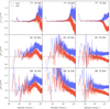 |
Fig. 14. Ratios between the angular auto-spectra shown in Fig. 12, adopting the BEYONDPLANCK spectra as reference. Planck 2018 results are shown as blue lines, while Planck PR4 results are shown as red lines. Values larger than unity imply that the respective map has more power than the corresponding BEYONDPLANCK spectrum. |
These effects explain the different white noise levels. However, they do not necessarily explain the different slopes of the spectra seen in Fig. 13, which instead indicate that the level of correlated noise is significantly lower in the BEYONDPLANCK maps as compared to the other two pipelines. The main reason for this is as follows: While Planck 2018 and PR4 both destripe each frequency map independently, BEYONDPLANCK effectively performs joint correlated noise estimation using all available frequencies at once, as described by BeyondPlanck Collaboration (2023) and Ihle et al. (2023). This is implemented in practice by conditioning on the current sky model during the correlated noise estimation phase in the Gibbs loop in Eqs. (4)–(11), which may be compared to the application of the destriping projection operator Z in the traditional pipelines that is applied independently to each channel. Intuitively, in the BEYONDPLANCK approach the 30 GHz channel is in effect helped by the 70 GHz channel to separate true CMB fluctuations from its correlated noise, while the 70 GHz channel is helped by the 30 GHz channel to separate synchrotron and free-free emission from its correlated noise. And both 30 and 70 GHz are helped by both WMAP and HFI to separate thermal and spinning dust from correlated noise. Of course, this also means that the correlated noise component are correlated between frequency channels, as discussed in Sect. 3, and it is therefore imperative to actually use the Monte Carlo samples themselves to propagate uncertainties faithfully throughout the system3.
6. Sample-based error propagation
As discussed in BeyondPlanck Collaboration (2023), one of the main motivations underlying the current Bayesian end-to-end analysis framework is to support robust and complete error propagation for current and next-generation CMB experiments, and we use the LFI data as a worked example. In this section, we discuss three qualitatively different manners in which the posterior samples may be used for this purpose, namely 1) post-processing of individual samples; 2) derivation of a low-resolution dense covariance matrix, and 3) half-mission half-difference maps. We discuss all three methods, and we start with an intuitive comparison of the Bayesian and the traditional approaches.
6.1. Bayesian posterior sampling versus frequentist simulations
Traditionally, CMB frequency maps are published in terms of a single maximum-likelihood map with an error description that typically takes one of two forms. We may call the first type “analytical,” and this usually takes the form of either a full-resolution but diagonal (i.e., “white noise”) or a low-resolution but dense covariance matrix, coupled with a single overall calibration factor and a limited number of multiplicative template-based corrections. This error description aims to approximate the covariance matrix defined by the inverse coupling matrix in Eq. (14), within the bounds of computational feasibility. The main advantage of this type of error estimate is that it may both be computed and propagated into higher-level analyses analytically.
The second type of classical error estimate may be referred to as “simulations”, and is defined in terms of an ensemble of end-to-end forward simulations. Each realization in this ensemble represents, ideally, one statistically independent set of specifications for all the astrophysical4 and instrumental (noise, systematics, scanning strategy) parameters; then, the simulated time-ordered data corresponding to this specification set is processed in an identical manner as the real data (e.g., Planck Collaboration XII 2016). To actually propagate uncertainties based on these simulations into higher-level products, one can either analyze each realization with the same statistics as the real data, and form a full histogram of test statistics, or use the simulations to first generate a covariance matrix, and then propagate that analytically through higher-level codes.
The Bayesian posterior sampling approach looks very similar to the traditional simulation approach in terms of output products: Both methods produce a large ensemble of sky map realizations that may be analyzed with whatever higher-level analysis statistics the end-user prefers. However, the statistical foundation and interpretation – and therefore their applicability – of the two methods are in fact very different: While the forward frequentist simulation approach considers a set of random instruments in a set of random universes, the Bayesian approach considers our instrument in our Universe; for an in-depth discussion regarding this issue, see Brilenkov et al. (2023).
The relevance and importance of this difference for actual CMB analysis applications may be illustrated by the following series of observations. Suppose we are tasked with generating an optimal simulation suite to analyze a given frequency map. One important question we have to address is, “what CMB dipole parameters should we adopt?” The importance of this question is highlighted in Fig. 11, which shows the differences between the BEYONDPLANCK and Planck maps; if completely random CMB Solar dipole parameters were used, the large coherent structures in these plots would move around randomly from realization to realization, to the extent that the simulated uncertainties would not actually be a useful description of our sky map. For this reason, all CMB analysis pipelines to date have actually used dipole parameters close to the real sky.
A second important question is, “what Galactic model should we use?” The same observations hold in this case; if one were to use random Galactic models for each simulation, the Galactic plane’s morphology in Fig. 11 would change from realization to realization, and no longer even be aligned with our Milky Way, and the simulated ensemble would obviously not be useful to describe the uncertainties in the real sky map. For this reason, all CMB pipelines to data have also adopted a Galactic model close to the real sky.
So far, the discussion has been rather straightforward. However, the next question that emerges is more controversial, namely “what CMB fluctuations should we use to generate the simulations?” In this case, most traditional pipelines actually adopt statistically independent Λ cold dark matter (CDM) realizations that have no coupling to the real sky. This component is thus treated logically very differently from the CMB dipole and the Galaxy, and this has important consequences for any correlation structures that result from the simulated ensemble; the simulations are no longer useful to describe the features seen in Fig. 11, simply because the coherence between the small-scale CMB fluctuations and the gain variations, the correlated noise, the foreground fluctuations etc., has been broken.
This issue does not only apply to the CMB fluctuations, but also to the instrument parameters. Of course, the basic knowledge of instrument parameters comes from hardware calibration measurements. However, these inevitably come with an uncertainty, and in the traditional approach these uncertainties are extremely difficult to propagate through the data analysis. So in some cases (e.g., bandpasses) the parameters are treated as fixed values in the pipeline, and the potential bias arising from the uncertainty in the hardware measurement is evaluated separately (see, e.g., Figs. 24–26 of Planck Collaboration XII 2016). This approach is able to quantify the potential impact of the systematic effect compared to the signal power spectra, but it does not control the correlation of the effect with other parameters (in this case, most notably, astrophysical foreground parameters) thus preventing a rigorous error analysis. In other cases, such as 1/f noise, the relevant parameters (e.g., gain change as a function of time, or “baseline”) are not derived from hardware measurements, but are chosen randomly from some hyper-distribution, independent from the real data. However, gain fluctuations correlate with the CMB dipole and fluctuations and the Galactic model, and consequently they may generate coherent features at very specific positions in the final frequency map.
In contrast to the frequentist forward simulation approach that uses random simulations to describe uncertainties, the Bayesian posterior sampling approach couples every single parameter to the actual data set in question, and treats the CMB fluctuations and instrument parameters on the same statistical footing as the CMB dipole and Galactic signal. Intuitively speaking, the Bayesian sampling approach is identical to the simulation approach, with the one important difference that the Bayesian method adopts a constrained realization to generate the end-to-end simulation for all parameters, while the frequentist approach uses a random realization (or a mixture of random and constrained realizations).
The conclusion from this set of observations is that the Bayesian and frequentist approaches actually addresses two fundamentally different questions (Brilenkov et al. 2023). The Bayesian samples are optimally tuned to answer questions like “what are the best-fit ΛCDM parameters of our specific data set?”, while the frequentist simulations are optimally tuned to answer questions like “is our data set consistent with the ΛCDM model?” The fundamental difference lies in whether the correlation structures between realizations are tuned to describe uncertainties in our specific instrument and Universe, or uncertainties in a random instrument in a random universe.
It is, however, clear that both the Bayesian posterior sampling and the frequentist simulation approaches have decisive practical advantages over the analytical method in terms of modeling complex systematic effects and their interplay. As a practical demonstration of this, Fig. 15 shows the difference between two BEYONDPLANCK frequency map samples for each frequency channel, smoothed to a common angular resolution of 7° FWHM. Here we clearly see correlated noise stripes along the Planck scan direction in all three frequency channels, as well as coherent structures along the Galactic plane. Clearly, modeling such correlated fluctuations in terms of a single standard deviation per pixel is inadequate, and, as we subsequently see in the next section, these structures also cannot be described as simply correlated 1/f noise. End-to-end analysis that simultaneously accounts for all sources of uncertainties is key for fully describing these uncertainties.
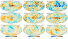 |
Fig. 15. Difference maps between two frequency map samples, smoothed to a common angular resolution of 7° FWHM. Rows show, from top to bottom, the 30, 44 and 70 GHz frequency channels, while columns show, from left to right, the temperature and Stokes Q and U parameters. Monopoles of 2.8, 1.6, and −0.5 μK have been subtracted from the three temperature components, respectively. |
6.2. Sample-based covariance matrix evaluation
For several important applications, including low-ℓ CMB likelihood evaluation (e.g., Page et al. 2007; Planck Collaboration V 2020; Paradiso et al. 2023), it is important to have access to full pixel-pixel covariance matrices. Since the memory required to store these scale as  , and the CPU time required to invert them scale as
  , (Sherman & Morrison 1950), these are typically only evaluated at very low angular resolution; Planck used Nside = 16 (Planck Collaboration V 2020), while BEYONDPLANCK uses Nside = 8 (Paradiso et al. 2023).
In the traditional approach, it is most common to primarily account for 1/f-type correlated noise, and the matrix may then be constructed by summing up the temporal two-point correlation function between any two sample pairs separated by some maximum correlation length. This calculation is implementationally straightforward, but expensive. In addition, an overall multiplicative calibration uncertainty may be added trivially, and spatially fixed template corrections (for instance for foregrounds or gain uncertainties; Planck Collaboration II 2020) may be accounted for through the Sherman-Morrison-Woodbury formula.
This analytical approach, however, is not able to account for more complex sources of uncertainty, perhaps most notably gain uncertainties that vary with detector and time (Gjerløw et al. 2023), but also more subtle effects such as sidelobe (Galloway et al. 2023b) or bandpass uncertainties (Svalheim et al. 2023), all of which contribute to the final total uncertainty budget. To account for these, end-to-end simulations – whether using random or constrained realizations – are essential. The resulting covariance matrix may then be constructed simply by averaging the pixel-pixel outer product over all samples,
 (17)
(17)
 (18)
(18)
In practice, we also follow Planck 2018, and add 2 μK (0.02 μK) Gaussian regularization noise to each pixel in temperature (polarization), in order to stabilize nearly singular modes that otherwise prevent stable matrix inversion and determinant evaluations.
The importance of complete error propagation is visually illustrated in Fig. 16, which compares an arbitrarily selected slice through the Planck 2018 LFI low-resolution covariance matrix that accounts only for 1/f correlated noise with the corresponding BEYONDPLANCK covariance matrix (Planck Collaboration V 2020). (Note that the two matrices are evaluated at different pixel resolution, and that the Planck 2018 matrix applies a cosine apodization filter that is not used in BEYONDPLANCK. Also, the TP cross-terms at 70 GHz are set to zero by hand in the Planck covariance matrices).
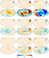 |
Fig. 16. Single column of the low-resolution 30 (top section), 44 (middle section), and 70 GHz (bottom section) frequency channel covariance matrix, as estimated analytically by the LFI DPC (top rows) and by posterior sampling in BEYONDPLANCK (bottom rows). The selected column corresponds to the Stokes Q pixel marked in gray, which is located in the top right quadrant in the BEYONDPLANCK maps. Note that the DPC covariance matrix is constructed at Nside = 16 and includes a cosine apodization filter, while the BEYONDPLANCK covariance matrix is constructed at Nside = 8 with no additional filter. The temperature components are smoothed to 20° FWHM in both cases, and Planck 2018 additionally sets the TQ and TU elements by hand to zero for the 70 GHz channel. |
When comparing these slices, two obvious qualitative differences stand out immediately. First, the BEYONDPLANCK matrices appear noisy, while the Planck appear smooth; this is because the former are constructed by Monte Carlo sampling, while the latter are constructed analytically. In practice, this means that any application of the BEYONDPLANCK covariance matrices must be accompanied with a convergence analysis that shows that the number of Monte Carlo samples is sufficient to reach robust results for the final statistic in question. How many this is will depend on the statistic in question; for an example of this as applied to estimation of the optical depth of reionization, see Paradiso et al. (2023). Second, and even more importantly, we also see that the BEYONDPLANCK matrices are far more feature rich than the Planck 2018 matrices, and this is precisely because they account for a full stochastic data model, and not just 1/f correlated noise.
This is most striking for the 30 GHz channel, for which it is in fact nearly impossible to see the 1/f imprint at all. Rather, the slice is dominated by a large-scale red-blue quadrupolar pattern aligned with the Solar dipole, and this is an archetypal signature of inter-detector calibration differences (see, e.g., Planck Collaboration II 2020; Gjerløw et al. 2023). A second visually striking effect is the Galactic plane, which is due to bandpass mismatch uncertainties (Svalheim et al. 2023). There are of course numerous other effects also present in these maps, although these are generally harder to identify visually.
Figure 17 shows the angular noise power spectra corresponding to these matrices (black for BEYONDPLANCK, and red for Planck 2018) in both temperature and polarization. For comparison, this plot also includes similar spectra computed from the end-to-end Planck PR4 simulations (blue). The dashed line shows the pure white noise contribution in the BEYONDPLANCK covariances, while the dotted line shows the best-fit Planck 2018 EEΛCDM spectrum.
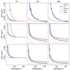 |
Fig. 17. Comparison of noise power spectra from BEYONDPLANCK (black), Planck 2018 (red) and PR4 (blue); We report the Planck 2018 best-fit with a dotted line, and the BEYONDPLANCK white noise contribution as a dashed line. Each dataset includes a regularization noise of 2 μK/pixel for temperature, and 0.02 μK/pixel for polarization. |
We first note that the temperature component of these covariance matrices is heavily processed by first convolving to 20° FWHM, and then adding uncorrelated regularization noise of 2 μK/pixel; this explains why all curves converge above ℓ ≈ 10 in temperature. Secondly, we note that Planck PR4 did not independently reestimate the LFI 1/f parameters, but rather adopted the Planck 2018 values for this. The difference between the blue and red curves (after taking into account the 15% lower white noise level in PR4) thus provides a direct estimate of the sum of other effects than correlated noise in Planck 2018, most notably gain uncertainties.
Overall, the BEYONDPLANCK polarization noise spectra agree well with Planck PR4 at 30 GHz, while they are generally lower by as much as 20–50% at 44 and 70 GHz. In fact, we see that the BEYONDPLANCK 70 GHz noise spectrum almost reaches the white noise floor around ℓ ≈ 20, suggesting that the current processing has succeeded in removing both excess correlated noise and gain fluctuations to an unprecedented level.
6.3. Half-mission split maps
Before concluding this section, we also consider error propagation by half-mission split maps, as such maps have been used extensively by all generations of the Planck pipelines (Planck Collaboration I 2014, 2016, 2020). These maps are generated by dividing the full data set into two disjoint sets, typically either by splitting each scanning period in two (resulting in half-ring maps); or by dividing the entire mission into two halves (resulting in half-mission maps); or by dividing detectors into separate groups (resulting in detector maps). The goal of each of these splits is the same, namely to establish maps with similar signal content, but statistically independent noise realizations. The resulting maps may then be used for various cross-correlation analyses, including power spectrum estimation (e.g., Planck Collaboration V 2020).
In general, the usage of cross-correlation techniques is an implicit admission that our understanding of the instrumental systematic effects is incomplete, and the main goal of the current BEYONDPLANCK processing is precisely to establish a statistically adequate error propagation model. As such, the primary CMB results presented by Colombo et al. (2023) and Paradiso et al. (2023) do not employ cross-correlation techniques at all, but rather rely fully on statistically optimal auto-spectrum estimation, in which all information is fully exploited. The current section is therefore included primarily for comparison purposes with respect to the original Planck processing.
Before presenting half-mission maps from BEYONDPLANCK, we note that Planck 2018 and PR4 adopted different conventions for how to split the mission into two halves. Specifically, while Planck 2018 simply divided the mission in two, and made separate maps for years 1 + 2 and 3 + 4, Planck PR4 instead chose to coadd years 1 + 3 and 2 + 4. The main reason for this is that years 3 + 4 do not result in full-sky coverage for the LFI maps, but leaves a small hole, which is awkward for cross-correlation analyses. The cost of this choice, however, is slightly less independent halves, which may lead to additional common modes. An important example of this is asymmetric beams; as discussed by Planck Collaboration I (2016), the scanning phase of the Planck satellite was reversed between years 2 and 3, and this adds additional beam symmetrization between the first and second half of the mission. Therefore, the effect of beam asymmetries is maximized in the Planck 2018 split, but minimized in the Planck PR4 split. In this paper, we choose to follow Planck 2018, and focus on years 1 + 2 versus 3 + 4 splits.
Technically speaking, half-mission maps may be generated very straightforwardly in the BEYONDPLANCK pipeline at the parameter file level (Galloway et al. 2023a), simply by restricting the start and end PID of the analysis. In this case, all parameters, including the calibration and foreground model, will be fitted independently in each data set. We generate such half-mission samples for each frequency channel and compute pairwise differences between these. This set of half-mission maps are denoted “full” in the following, indicating that the full model is fitted in each half-mission set.
However, it is important to note that this mode differs significantly from the official Planck implementation. Rather, in the Planck 2018 case, both the calibration and foreground model are fixed at their full-mission values, while in the case of Planck PR4, the foreground model is fixed, and the calibration model is reestimated. To mimic the Planck 2018 behavior, we therefore create a second set of BEYONDPLANCK half-mission maps, in which all model parameters except the correlated noise are fixed at their full mission values. We refer to this set as “conditional” (or “cond”) in the following, indicating that most parameters are in fact conditioned during generation.
Figure 18 shows half-mission half-difference maps (mhmhd = (m1 − m2)/2) for the LFI 30 GHz channel for all four cases, all smoothed to a common angular resolution of 5°. (Similar plots for the 44 and 70 GHz channels look qualitatively similar, and is omitted for brevity). Starting with the two bottom rows that show BEYONDPLANCK “cond” and “full”, respectively, we see that conditioning on the calibration and foreground parameters has a substantial impact in terms of overall variations. The typical large-scale fluctuation level is at least a factor of two larger when fitting all parameters freely, and there is significantly more pronounced coherent large-scale features. We also see that these two cases (at least in temperature) bound the Planck 2018 and PR4 cases, in the sense that the fluctuations generally increase as more and more parameters are refitted; the main difference between Planck PR4 and BEYONDPLANCK is a large-scale quadrupole pattern, which looks very much like the familiar bandpass residuals are seen by both Planck 2018 and PR4 (Planck Collaboration Int. LVII 2020), and may originate from the foreground and/or beam differences.
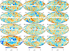 |
Fig. 18. Half mission difference maps for the 30 GHz channel. The top row shows the Planck data release 3 maps, while the second top row shows the difference for the Planck data release 4 maps. The bottom two rows show BP maps. The third row shows the first sample of a conditional run on astrophysical and instrumental parameters. The bottom row shows the difference between the half mission maps made from two independent runs that sample over the full model. The latter maps are averaged over 50 samples. |
In polarization, this trend is less obvious, as in this case the absolute magnitude of the pipeline-specific residuals is comparable with the level from parameter conditioning. In this case, the BEYONDPLANCK “cond” case shows clearly smaller differences than either of the two Planck implementations, while the “full” case shows comparable levels.
The sky maps shown in Fig. 18 emphasize the very largest angular scales. To obtain additional information regarding intermediate and small scales, we show in Fig. 19 the auto-spectra of each case. For comparison, the dashed curve shows the beam-convolved best-fit ΛCDM spectrum for each channel. Starting with the noise-dominated polarization spectra, we see that all four pipelines result in roughly similar half-mission power, and this indicates that their abilities to propagate and describe instrumental noise alone are very similar. For temperature, the picture is qualitatively different, and there is a strong excess from the sky signal, most notably at 30 GHz, that appears to fall off with the beam smoothing. The fact that Planck 2018 and BEYONDPLANCK appears nearly identical in this case, while Planck PR4 is substantially lower, strongly suggests that asymmetric beams can account for at least some of this additional power. At the same time, the fact that BEYONDPLANCK “full” and “cond” differ shows that gain fluctuations also play a significant role in explaining the full excess. However, the main conclusion from these results is that Planck 2018 and BEYONDPLANCK appear to perform similarly in terms of half-mission power on small scales, and this strongly suggests that both pipelines are likely to be close to the theoretical noise limit.
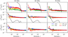 |
Fig. 19. Half-mission half-difference power spectra estimated by Planck 2018 (blue), Planck PR4 (green), and BEYONDPLANCK. In the case of BEYONDPLANCK, orange curves show spectra obtained from maps that are calibrated jointly (or “conditionally” with respect to the signal model), while red curves show spectra from maps that are processed completely independently. Columns show 30, 44, and 70 GHz results, while rows show TT, EE, and BB spectra. The dashed black line shows the best-fit Planck 2018 ΛCDM spectrum convolved with the instrument beam. |
7. Systematic error corrections and uncertainties
A significant strength of the novel Bayesian end-to-end framework is that all TOD contributions are modeled in terms of specific and physically motivated parametric models, and there are very few “black boxes” that can hide not understood contaminants; any contribution is either present in one of the parametric components, or it shows up in the TOD residual maps. This physical foundation is useful both when interpreting the results, and when debugging and tuning the analysis configuration. In this section, we provide a concrete example of this by presenting a complete survey of each systematic correction term, both in the form of projected sky maps and as residual power spectra, for all three LFI channels.
7.1. Sky map corrections
We start by showing projected systematic effect sky maps at 30 GHz, as summarized in Fig. 20. The top panel shows the raw TOD binned into a sky map, and this provides intuition regarding the overall quality of the data before applying any corrections. Indeed, for the temperature component it is very difficult to spot major artifacts of any kind; the most notable feature is a few correlated noise stripes in the lower left quadrant. For polarization, the dominant effect is the alternating sign along the Galactic plane as a function of longitude, which is due to bandpass mismatch.
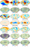 |
Fig. 20. Comparison between TOD corrections for the 30 GHz channel for a single Gibbs sample, projected into sky maps. Columns show Stokes T, Q, and U parameters. Rows show, from top to bottom, 1) raw TOD; 2) correlated noise; 3) the orbital dipole; 4) bandpass and beam mismatch leakage; 5) sidelobe corrections; and 6) 1 Hz electronic spike correction. The bottom row shows the shows the residual obtained when binning the sky and systematics subtracted TOD into a sky map. Note that some components have been smoothed to an angular resolution of 1° FWHM. |
The second panel shows the correlated noise component. The most notable features in this map are coherent stripes along the satellite scanning path. It should also be noted that this component is the one that is the least constrained from a priori considerations among all TOD components, and therefore acts as a “trash can” for possible unmodeled errors; this is the first place one expects to see residuals from modeling errors. The fact that this appears statistically clean, and has a morphology that is close to that actually expected by 1/f-type correlated noise provides very strong evidence that the current processing has succeeded in cleaning the 30 GHz channel with respect to most systematic effects.
The third row shows the orbital dipole. For a single PID, this signal is defined by a perfect dipole along the scanning ring with an amplitude of about 270 μK, convolved with the 4π LFI beam. However, when the same ring is observed six months apart, the phase of the signal is reversed, and the total gain- and noise-weighted sum is then both smaller and difficult to predict. Also, although the intrinsic signal is entirely unpolarized, convolution with far-sidelobes algebraically couples this model to the polarization sector as well. Because of the relatively large amplitude of this signal, and the fact that it has no free parameters to be fitted in the pipeline, the orbital dipole represents our best available tracer of gain fluctuations.
The fourth row shows the bandpass and beam leakage correction. This effect is clearly the strongest among all polarization corrections, with amplitudes of many tens of μK in the Galactic plane, while still being almost entirely negligible in temperature. Morphologically speaking, the archetypal signature of bandpass mismatch is a variable sign along the Galactic plane, tracing the specific orientation of the detector polarization angles as the different detectors observe at slightly different effective frequencies. At high latitudes, this map is dominated by temperature-to-polarization leakage resulting from different radiometers observing the signal model with different beam FWHMs; large angular scales are dominated by CMB dipole leakage, while small angular scales are dominated by foregrounds and CMB temperature fluctuations.
The fifth row shows the impact of sidelobe pickup. In temperature, the two dominant features are, first, a large-scale pattern broadly aligned with the solar CMB dipole resulting from interactions with the intermediate sidelobes, and, second, individual rings created by the far sidelobes hitting the Galactic plane. The same features are also seen in polarization, but now a more complicated pattern arises due to the additional modulation by the relative orientation of the polarization angles at any given time.
The sixth row shows the contribution from electronic 1 Hz spikes. Two points are important to note regarding this signal. First and foremost, the color bar only spans 0.3 μK, and this term is thus very small in absolute magnitude compared to all other, in agreement with the Planck 2018 analysis. Second, this signal is also primarily located on small angular scales, and looks almost like white noise at the level of sky maps.
The last row shows the TOD residuals binned into a sky map. For most of the sky, this is consistent with white noise, but clear residuals are seen in the Galactic plane, reflecting the structures seen in the bottom panel of Fig. 1. This indicates that the adopted foreground and/or instrument model is not statistically adequate in these very bright regions of the sky, and all higher-level CMB-oriented analyses should obviously mask these regions prior to power spectrum or parameter estimation. However, the main conclusion to be drawn from this plot is indeed that the parametric data model summarized in the above panels is very efficient at describing the raw LFI TOD at 30 GHz.
For completeness, Figs. 21 and 22 show corresponding surveys for the 44 and 70 GHz channels. Overall, these behave very similarly as the 30 GHz channel, with minor variations. For instance, we see that the bandpass corrections are much smaller at the two higher frequencies, while the sidelobe correction is particularly low at 44 GHz, es expected from the optical analysis (Sandri et al. 2010). On the other hand, the electronic 1 Hz spike signal is larger at 44 GHz than either of the other two channels, but still very small compared to all other terms. Most importantly, however, we see once again that the correlated noise and TOD residual maps appear visually clean of large systematic effects at high Galactic latitudes, and this demonstrates that the parametric model is able to describe also the 44 and 70 GHz TODs to a very high precision.
7.2. Power spectrum residuals
The maps shown in Figs. 20–22 provide useful intuition regarding the typical amplitude of each systematic effect, but they do not provide an estimate of the residual uncertainty associated with each effect. To quantify these residuals, we first compute the mean of each effect across the full posterior ensemble, and subtract this from each individual Gibbs sample. We then compute the (pseudo-)power spectrum of each effect, adopting the CMB analysis mask presented by Colombo et al. (2023), while correcting for the masked sky fraction. We then plot the standard deviation of the resulting power spectra in Fig. 23 for each frequency and each polarization spectrum. For comparison, we also plot the power spectrum of the full posterior mean map (thick black curves); the standard deviation of the same across all samples (thick red curves); the white noise level of each channel (thick gray curves); and the best-fit Planck 2018 ΛCDM spectrum (dashed black curves). Thus, this plot provides a fairly comprehensive description of the various systematic uncertainties modeled by the BEYONDPLANCK pipeline.
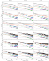 |
Fig. 23. Pseudo-spectrum standard deviation for each instrumental systematic correction shown in Figs. 20–22 (thin colored lines). For comparison, thick black lines show spectra for the full coadded frequency map; thick red lines show the standard deviation of the same (i.e., the full systematic uncertainty); gray lines show white noise; and dashed black lines show the best-fit Planck 2018 ΛCDM power spectrum convolved with the instrument beam. Columns show results for 30, 44 and 70 GHz, respectively, while rows show results for each of the six polarization states (TT, EE, BB, TE, TB, and EB). All spectra have been derived outside the CMB confidence mask presented by Andersen et al. (2023) using the HEALPix anafast utility, correcting only for sky fraction and not for mask mode coupling. |
Starting with the 30 GHz TT spectrum, we first note that the posterior mean sky map (thick black) is reasonably well modeled by CMB (dashed black) and white noise (thick gray) above ℓ ≈ 100. At lower multipoles, there is a notable excess compared to ΛCDM, and this may be explained in terms of contributions from diffuse Galactic foregrounds; this discrepancy is much smaller at 44 and 70 GHz.
The red curve shows the sum of all systematic error corrections. In TT, this exceeds white noise below ℓ ≲ 100–150, depending on channel, while for EE it dominates for ℓ ≲ 20 at 30 GHz, and for ℓ ≲ 7–8 at 70 GHz. The dominant systematic uncertainty in EE at 70 GHz on the very largest scales is the orbital dipole (blue curves), which implies gain fluctuations, as already noted through visual inspection of the low-resolution covariance matrices in Sect. 6; in comparison, the contribution from correlated noise (orange curve) is about an order of magnitude smaller at these ℓs.
This only holds true at 70 GHz, however. Both at 30 and 44 GHz, the gain and correlated noise fluctuations are comparable in magnitude in EE, and at 30 GHz also the bandpass leakage variations (thin red curve) are of the same order of magnitude. In contrast, this effect is completely negligible at both 44 and 70 GHz.
Next, we see that the sidelobe contribution (green curves) also appears subdominant at all scales in all frequencies. However, this picture is incomplete for at least two reasons. First of all, as discussed by Galloway et al. (2023b), uncertainties in the actual sidelobe response function is not propagated in the current pipeline, and support for this must clearly be added in a future extension of the framework. Second, this plot does not account for the overall mean sidelobe corrections, which, as seen in Figs. 20–22, has a strong coupling to the CMB Solar dipole, and thereby the overall calibration, which is accounted for in the red (orbital dipole) curve. Therefore, the green curve in this particular figure should not be interpreted as sidelobes being irrelevant. On the contrary, sidelobes are important, and their coupling to the calibration serves as a useful reminder that the entire analysis process is indeed global in nature, and marginal distributions, like those shown in Fig. 23, offers a limited view of the full joint distribution. Only the full sample set provides a complete description of the full posterior.
8. Conclusions
In this paper, we have presented novel Planck LFI frequency maps as derived through the Bayesian BEYONDPLANCK end-to-end analysis pipeline. These maps have both lower absolute residual systematic uncertainties than the corresponding Planck 2018 products, and a substantially more complete characterization of those residual uncertainties. One important example of the former is the fact that the absolute calibration uncertainty for BEYONDPLANCK is, at least nominally, 25–40 times lower than that of Planck 2018, while an important example of the latter is provided by the low-resolution covariance matrices of each pipeline; the BEYONDPLANCK covariances include all modeled sources of uncertainty, while the Planck 2018 covariance matrices only include correlated noise and a few template-based corrections for gain and foregrounds.
These advances have been made possible through the development of the first end-to-end CMB analysis pipeline, implemented in the form of a statistically well-defined Gibbs sampler. The main advantage of this framework is that all parameters, including relevant instrumental parameters, are explored jointly, both in terms of individual frequency channels and model parameters. Explicitly, rather than first calibrating and binning each frequency channel separately, and then performing component separation frequency maps, the current method performs calibration, mapmaking, and component separation in one tightly integrated iterative loop in which all parameters communicate directly with each other.
The importance of the end-to-end approach is clearly demonstrated by a careful analysis of the uncertainty budget of residual systematics for LFI. For the 70 GHz EE spectrum, for instance, we show that the dominant low-multipole systematic effect is actually detector- and time-dependent gain variations, and not 1/f-type correlated noise. For the 30 GHz channel, gain, bandpass, and correlated noise uncertainties are all of comparable order of magnitude. These effects are difficult to account for through traditional approaches, but easy to model in an a tightly integrated pipeline.
We also argue that the novel Bayesian approach presented here has a fundamentally different statistical interpretation than the traditional frequentist simulation approach adopted by most experiments to date. While both approaches are indeed able to model and propagate systematic uncertainties using end-to-end simulations, the fundamental difference lies in what parameters are assumed when generating the simulated TOD in the first place. In the traditional approach some astrophysical and instrumental parameters are assumed at the start of the analysis with no formal propagation of their errors; other parameters are drawn from random distributions and propagated through the pipeline with no realistic reference to our knowledge of their values. Conversely, in the novel Bayesian approach, all parameters are derived as constrained realization from the real dataset. On the other hand, we also note that even the traditional approach typically adopts constrained realizations for some key parameters, most importantly the CMB Solar dipole and the diffuse Galactic model, and this makes its statistical interpretation somewhat nontrivial. Focusing on the main CMB anisotropies, however, we argue that the two approaches fundamentally address different questions. The Bayesian approach is optimally tuned to answer questions like “what are the best-fit ΛCDM parameters of our universe?”, while the frequentist approach is optimally tuned to answer questions like “is our dataset compatible with ΛCDM?” For further details on this topic, see Brilenkov et al. (2023).
Clearly, after more than two decades of building powerful community-wide analysis tools to analyze frequentist-style sky maps and simulations, it will require a few code adjustments before the new posterior-based products presented here will be used as widely as the traditional products. The main difference is fortunately straightforward: Rather than computing a given statistic from a single best-fit sky map, one should now estimate the same statistic from an ensemble of maps; for the current BEYONDPLANCK LFI processing, this ensemble consists of 3200 individual maps. As such, code parallelization will be an important task going forward, but, fortunately, for many codes this has already been done in order to analyze the end-to-end simulations provided by Planck. If so, generalization to the Bayesian approach is indeed straightforward.
Both the current BEYONDPLANCK code base and the associated LFI products are made publicly available (Gerakakis et al. 2023), and generalization to various other datasets is currently ongoing. The most advanced of these is WMAP, as reported by Watts et al. (2023), for which significant improvements are found with respect to the official processing. COSMOGLOBE5 is an Open Source initiative aiming to coordinate such work for a wide range of experiments and datasets, and we highly encourage everybody interested to participate in this community-wide effort.
We note that the current Commander3 implementation only outputs the diagonal of the 3 × 3 noise covariance; the off-diagonal elements will be added in a future update.
It must of course be noted that the traditional pipelines also exhibit a correlated noise component between different frequencies, simply because they use the same foreground sky model to estimate bandpass and gain corrections at different frequencies. This, however, is very difficult to both quantify or propagate, because of the substantial cost of including full component separation within a forward simulation pipeline.
In practice, the astrophysical sky model is often kept fixed between realizations for pragmatic reasons.
Acknowledgments
We thank Prof. Pedro Ferreira and Dr. Charles Lawrence for useful suggestions, comments and discussions. We also thank the entire Planck and WMAP teams for invaluable support and discussions, and for their dedicated efforts through several decades without which this work would not be possible. The current work has received funding from the European Union’s Horizon 2020 research and innovation programme under grant agreement numbers 776282 (COMPET-4; BEYONDPLANCK), 772253 (ERC; BITS2COSMOLOGY), and 819478 (ERC; COSMOGLOBE). In addition, the collaboration acknowledges support from ESA; ASI and INAF (Italy); NASA and DoE (USA); Tekes, Academy of Finland (grant no. 295113), CSC, and Magnus Ehrnrooth foundation (Finland); RCN (Norway; grant nos. 263011, 274990); and PRACE (EU).
References
- Andersen, K. J., Herman, D., Aurlien, R., et al.), 2023, A&A, 675, A13 (BeyondPlanck SI) [NASA ADS] [CrossRef] [EDP Sciences] [Google Scholar]
- Ashdown, M. A. J., Baccigalupi, C., Balbi, A., et al. 2007, A&A, 471, 361 [NASA ADS] [CrossRef] [EDP Sciences] [Google Scholar]
- Bennett, C. L., Bay, M., Halpern, M., et al. 2003, ApJ, 583, 1 [NASA ADS] [CrossRef] [Google Scholar]
- BeyondPlanck Collaboration (Andersen, K. J., et al.) 2023, A&A, 675, A1 (BeyondPlanck SI) [Google Scholar]
- Brilenkov, M., Fornazier, K. S. F., Hergt, L. T., et al. 2023, A&A, 675, A4 (BeyondPlanck SI) [NASA ADS] [CrossRef] [EDP Sciences] [Google Scholar]
- Burigana, C., Malaspina, M., Mandolesi, N., et al. 1999, ArXiv e-prints [arXiv:astro-ph/9906360] [Google Scholar]
- Chon, G., Challinor, A., Prunet, S., Hivon, E., & Szapudi, I. 2004, MNRAS, 350, 914 [Google Scholar]
- Colombo, L. P. L., Eskilt, J. R., Paradiso, S., et al. 2023, A&A, 675, A11 (BeyondPlanck SI) [NASA ADS] [CrossRef] [EDP Sciences] [Google Scholar]
- Delabrouille, J. 1998, A&AS, 127, 555 [NASA ADS] [CrossRef] [EDP Sciences] [Google Scholar]
- Delouis, J. M., Pagano, L., Mottet, S., Puget, J. L., & Vibert, L. 2019, A&A, 629, A38 [NASA ADS] [CrossRef] [EDP Sciences] [Google Scholar]
- Fixsen, D. J. 2009, ApJ, 707, 916 [Google Scholar]
- Galloway, M., Andersen, K. J., Aurlien, R., et al. 2023a, A&A, 675, A3 (BeyondPlanck SI) [NASA ADS] [CrossRef] [EDP Sciences] [Google Scholar]
- Galloway, M., Reinecke, M., Andersen, K. J., et al. 2023b, A&A, 675, A8 (BeyondPlanck SI) [NASA ADS] [CrossRef] [EDP Sciences] [Google Scholar]
- Geman, S., & Geman, D. 1984, IEEE Trans. Pattern Anal. Mach. Intell., 6, 721 [CrossRef] [Google Scholar]
- Gerakakis, S., Brilenkov, M., Ieronymaki, M., et al. 2023, Open J. Astrophys., 6, 10 [NASA ADS] [Google Scholar]
- Gjerløw, E., Ihle, H. T., Galeotta, S.., et al. 2023, A&A, 675, A7 (BeyondPlanck SI) [NASA ADS] [CrossRef] [EDP Sciences] [Google Scholar]
- Górski, K. M., Hivon, E., Banday, A. J., et al. 2005, ApJ, 622, 759 [Google Scholar]
- Ihle, H. T., Bersanelli, M., Franceschet, C., et al. 2023, A&A, 675, A6 (BeyondPlanck SI) [NASA ADS] [CrossRef] [EDP Sciences] [Google Scholar]
- Jewell, J., Levin, S., & Anderson, C. H. 2004, ApJ, 609, 1 [Google Scholar]
- Keihänen, E., Kurki-Suonio, H., Poutanen, T., Maino, D., & Burigana, C. 2004, A&A, 428, 287 [NASA ADS] [CrossRef] [EDP Sciences] [Google Scholar]
- Keihänen, E., Kurki-Suonio, H., & Poutanen, T. 2005, MNRAS, 360, 390 [NASA ADS] [CrossRef] [Google Scholar]
- Keihänen, E., Keskitalo, R., Kurki-Suonio, H., Poutanen, T., & Sirviö, A. S. 2010, A&A, 510, A57 [CrossRef] [EDP Sciences] [Google Scholar]
- Kurki-Suonio, H., Keihänen, E., Keskitalo, R., et al. 2009, A&A, 506, 1511 [NASA ADS] [CrossRef] [EDP Sciences] [Google Scholar]
- Maino, D., Burigana, C., Górski, K. M., Mandolesi, N., & Bersanelli, M. 2002, A&A, 387, 356 [NASA ADS] [CrossRef] [EDP Sciences] [Google Scholar]
- Maino, D., Burigana, C., Maltoni, M., et al. 1999, A&AS, 140, 383 [NASA ADS] [CrossRef] [EDP Sciences] [Google Scholar]
- Mather, J. C. 1982, Opt. Eng., 21, 769 [NASA ADS] [CrossRef] [Google Scholar]
- Mennella, A., Bersanelli, M., Butler, R. C., et al. 2010, A&A, 520, A5 [NASA ADS] [CrossRef] [EDP Sciences] [Google Scholar]
- Page, L., Hinshaw, G., Komatsu, E., et al. 2007, ApJS, 170, 335 [Google Scholar]
- Paradiso, S., Colombo, L. P. L., Andersen, K. J., et al. 2023, A&A, 675, A12 (BeyondPlanck SI) [NASA ADS] [CrossRef] [EDP Sciences] [Google Scholar]
- Planck Collaboration I. 2014, A&A, 571, A1 [NASA ADS] [CrossRef] [EDP Sciences] [Google Scholar]
- Planck Collaboration II. 2014, A&A, 571, A2 [NASA ADS] [CrossRef] [EDP Sciences] [Google Scholar]
- Planck Collaboration I. 2016, A&A, 594, A1 [NASA ADS] [CrossRef] [EDP Sciences] [Google Scholar]
- Planck Collaboration II. 2016, A&A, 594, A2 [NASA ADS] [CrossRef] [EDP Sciences] [Google Scholar]
- Planck Collaboration X. 2016, A&A, 594, A10 [NASA ADS] [CrossRef] [EDP Sciences] [Google Scholar]
- Planck Collaboration XII. 2016, A&A, 594, A12 [NASA ADS] [CrossRef] [EDP Sciences] [Google Scholar]
- Planck Collaboration XXV. 2016, A&A, 594, A25 [NASA ADS] [CrossRef] [EDP Sciences] [Google Scholar]
- Planck Collaboration I. 2020, A&A, 641, A1 [NASA ADS] [CrossRef] [EDP Sciences] [Google Scholar]
- Planck Collaboration II. 2020, A&A, 641, A2 [NASA ADS] [CrossRef] [EDP Sciences] [Google Scholar]
- Planck Collaboration III. 2020, A&A, 641, A3 [NASA ADS] [CrossRef] [EDP Sciences] [Google Scholar]
- Planck Collaboration IV. 2020, A&A, 641, A4 [NASA ADS] [CrossRef] [EDP Sciences] [Google Scholar]
- Planck Collaboration V. 2020, A&A, 641, A5 [NASA ADS] [CrossRef] [EDP Sciences] [Google Scholar]
- Planck Collaboration Int. LVII. 2020, A&A, 643, A42 [NASA ADS] [CrossRef] [EDP Sciences] [Google Scholar]
- Rocha, G., Keskitalo, R., Partridge, B., et al. 2023, A&A, 669, A92 [NASA ADS] [CrossRef] [EDP Sciences] [Google Scholar]
- Sandri, M., Villa, F., Bersanelli, M., et al. 2010, A&A, 520, A7 [NASA ADS] [CrossRef] [EDP Sciences] [Google Scholar]
- Sherman, J., & Morrison, W. J. 1950, Ann. Math. Stat., 21, 124 [CrossRef] [Google Scholar]
- Svalheim, T. L., Zonca, A., Andersen, K. J., et al. 2023, A&A, 675, A9 (BeyondPlanck SI) [NASA ADS] [CrossRef] [EDP Sciences] [Google Scholar]
- Tegmark, M., Taylor, A. N., & Heavens, A. F. 1997, ApJ, 480, 22 [NASA ADS] [CrossRef] [Google Scholar]
- Wandelt, B. D., Larson, D. L., & Lakshminarayanan, A. 2004, Phys. Rev. D, 70, 083511 [Google Scholar]
- Watts, D. J., Galloway, M., Ihle, H. T., et al. 2023, A&A, 675, A16 (BeyondPlanck SI) [NASA ADS] [CrossRef] [EDP Sciences] [Google Scholar]
- Zacchei, A., Maino, D., Baccigalupi, C., et al. 2011, A&A, 536, A5 [NASA ADS] [CrossRef] [EDP Sciences] [Google Scholar]
- Zonca, A., Franceschet, C., Battaglia, P., et al. 2009, J. Instrum., 4, 2010 [Google Scholar]
All Tables
All Figures
|
Fig. 1. Time-ordered data segment for the 30 GHz LFI 27M radiometer. From top to bottom, the panels show 1) raw calibrated TOD, d/g; 2) sky signal, ssky; 3) calibrated correlated noise, ncorr/g; 4) orbital CMB dipole signal, sorb; 5) sidelobe correction, ssl; 6) electronic 1 Hz spike correction, s1 Hz; 7) leakage mismatch correction, sleak; and 8) residual TOD, dres = (d − ncorr − s1 Hz)/g − ssky − sorb − sleak − ssl. |
| In the text | |
|
Fig. 2. Trace plots of a set of selected frequency map parameters and related quantities; see main text for full definitions. The different colors indicate two independent Gibbs chains, and the 340 and 1960 subscripts indicate HEALPix pixel numbers at resolution Nside = 16 in ring ordering. |
| In the text | |
|
Fig. 3. Correlation coefficients between the same parameters as shown in Fig. 2. The subscripts a and b relate to the 340 and 1960 HEALPix pixel numbers. The lower triangle shows raw correlations, while the upper triangle shows correlations after high-pass filtering with a running mean with a 10-sample window. For further explanation of and motivation for this filtering, see Andersen et al. (2023). |
| In the text | |
|
Fig. 4. Posterior mean maps for the 30 GHz frequency channel. From top to bottom: Stokes I, Q and U parameters. Maps have resolution Nside = 512, are presented in Galactic coordinates, and polarization maps have been smoothed to an effective angular resolution of 1° FWHM. |
| In the text | |
|
Fig. 5. Posterior mean maps for the 44 GHz frequency channel. From top to bottom: Stokes I, Q and U parameters. Maps have resolution Nside = 512, are presented in Galactic coordinates, and the polarization maps have been smoothed to an effective angular resolution of 1° FWHM. |
| In the text | |
|
Fig. 6. Posterior mean maps for the 70 GHz frequency channel. From top to bottom: Stokes I, Q and U parameters. Maps have a HEALPix resolution of Nside = 1024, are presented in Galactic coordinates, and the polarization maps have been smoothed with a FWHM = 1° Gaussian beam. |
| In the text | |
|
Fig. 7. Posterior standard deviation maps for each LFI frequency. Rows show, from top to bottom, the 30, 44 and 70 GHz frequency channels, while columns show, from left to right, the temperature and Stokes Q and U parameters. The 30 GHz standard deviation is divided by a factor of 3. Note that these maps do not include uncertainty from instrumental white noise, but only variations from the TOD-oriented parameters included in the data model in Eq. (1). |
| In the text | |
|
Fig. 8. White noise standard deviation maps for a single arbitrarily selected sample. Rows show, from top to bottom, the 30, 44 and 70 GHz frequency channels, while columns show, from left to right, the temperature and Stokes Q and U parameters. Note that the 70 GHz maps are scaled by a factor of 2, to account for the fact that this map is pixelized at Nside = 1024, while the two lower frequencies are pixelized at Nside = 512. |
| In the text | |
|
Fig. 9. Posterior mean total data-minus-model residual maps rν = dν − sν for BEYONDPLANCK LFI 30 (top), 44 (middle), and 70 GHz (bottom). All maps are smoothed to a common angular resolution of 2° FWHM. |
| In the text | |
|
Fig. 10. Previously undetected TOD artifacts found by visual inspection of the (preliminary) correlated noise map for the 44 GHz channel shown in the top panel. The middle and lower panels show a zoom-in of the source PIDs, namely PID 6144 (for the “triangle feature”) and PID 14 416 (for the “dashed stripe feature”). In the two latter, the black curve shows the TOD residual, d − stot, for each sample, and the red curve shows the same after boxcar averaging with a 1 s window. |
| In the text | |
|
Fig. 11. Differences between BEYONDPLANCK and 2018 or PR4 frequency maps, smoothed to a common angular resolution of 2° FWHM. Columns show Stokes T, Q and U parameters, respectively, while rows show pair-wise differences with respect to the pipeline indicated in the panel labels. A constant offset has been removed from the temperature maps, while all other modes are retained. The 2018 maps have been scaled by their respective beam normalization prior to subtraction. |
| In the text | |
|
Fig. 12. Comparison between angular auto-spectra computed from the BEYONDPLANCK (black), Planck 2018 (blue), and PR4 (red) full-frequency maps. Rows show different frequencies, while columns show TT, EE, and BB spectra. All spectra have been estimated with PolSpice using the Planck 2018 common component separation confidence mask (Planck Collaboration IV 2020). |
| In the text | |
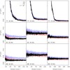 |
Fig. 13. Same as Fig. 12, but zooming in on the noise-dominated high-ℓ multipole range. |
| In the text | |
|
Fig. 14. Ratios between the angular auto-spectra shown in Fig. 12, adopting the BEYONDPLANCK spectra as reference. Planck 2018 results are shown as blue lines, while Planck PR4 results are shown as red lines. Values larger than unity imply that the respective map has more power than the corresponding BEYONDPLANCK spectrum. |
| In the text | |
|
Fig. 15. Difference maps between two frequency map samples, smoothed to a common angular resolution of 7° FWHM. Rows show, from top to bottom, the 30, 44 and 70 GHz frequency channels, while columns show, from left to right, the temperature and Stokes Q and U parameters. Monopoles of 2.8, 1.6, and −0.5 μK have been subtracted from the three temperature components, respectively. |
| In the text | |
|
Fig. 16. Single column of the low-resolution 30 (top section), 44 (middle section), and 70 GHz (bottom section) frequency channel covariance matrix, as estimated analytically by the LFI DPC (top rows) and by posterior sampling in BEYONDPLANCK (bottom rows). The selected column corresponds to the Stokes Q pixel marked in gray, which is located in the top right quadrant in the BEYONDPLANCK maps. Note that the DPC covariance matrix is constructed at Nside = 16 and includes a cosine apodization filter, while the BEYONDPLANCK covariance matrix is constructed at Nside = 8 with no additional filter. The temperature components are smoothed to 20° FWHM in both cases, and Planck 2018 additionally sets the TQ and TU elements by hand to zero for the 70 GHz channel. |
| In the text | |
|
Fig. 17. Comparison of noise power spectra from BEYONDPLANCK (black), Planck 2018 (red) and PR4 (blue); We report the Planck 2018 best-fit with a dotted line, and the BEYONDPLANCK white noise contribution as a dashed line. Each dataset includes a regularization noise of 2 μK/pixel for temperature, and 0.02 μK/pixel for polarization. |
| In the text | |
|
Fig. 18. Half mission difference maps for the 30 GHz channel. The top row shows the Planck data release 3 maps, while the second top row shows the difference for the Planck data release 4 maps. The bottom two rows show BP maps. The third row shows the first sample of a conditional run on astrophysical and instrumental parameters. The bottom row shows the difference between the half mission maps made from two independent runs that sample over the full model. The latter maps are averaged over 50 samples. |
| In the text | |
|
Fig. 19. Half-mission half-difference power spectra estimated by Planck 2018 (blue), Planck PR4 (green), and BEYONDPLANCK. In the case of BEYONDPLANCK, orange curves show spectra obtained from maps that are calibrated jointly (or “conditionally” with respect to the signal model), while red curves show spectra from maps that are processed completely independently. Columns show 30, 44, and 70 GHz results, while rows show TT, EE, and BB spectra. The dashed black line shows the best-fit Planck 2018 ΛCDM spectrum convolved with the instrument beam. |
| In the text | |
|
Fig. 20. Comparison between TOD corrections for the 30 GHz channel for a single Gibbs sample, projected into sky maps. Columns show Stokes T, Q, and U parameters. Rows show, from top to bottom, 1) raw TOD; 2) correlated noise; 3) the orbital dipole; 4) bandpass and beam mismatch leakage; 5) sidelobe corrections; and 6) 1 Hz electronic spike correction. The bottom row shows the shows the residual obtained when binning the sky and systematics subtracted TOD into a sky map. Note that some components have been smoothed to an angular resolution of 1° FWHM. |
| In the text | |
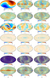 |
Fig. 21. Same as Fig. 20, but for the 44 GHz channel. |
| In the text | |
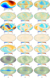 |
Fig. 22. Same as Fig. 20, but for the 70 GHz channel. |
| In the text | |
|
Fig. 23. Pseudo-spectrum standard deviation for each instrumental systematic correction shown in Figs. 20–22 (thin colored lines). For comparison, thick black lines show spectra for the full coadded frequency map; thick red lines show the standard deviation of the same (i.e., the full systematic uncertainty); gray lines show white noise; and dashed black lines show the best-fit Planck 2018 ΛCDM power spectrum convolved with the instrument beam. Columns show results for 30, 44 and 70 GHz, respectively, while rows show results for each of the six polarization states (TT, EE, BB, TE, TB, and EB). All spectra have been derived outside the CMB confidence mask presented by Andersen et al. (2023) using the HEALPix anafast utility, correcting only for sky fraction and not for mask mode coupling. |
| In the text | |
Current usage metrics show cumulative count of Article Views (full-text article views including HTML views, PDF and ePub downloads, according to the available data) and Abstracts Views on Vision4Press platform.
Data correspond to usage on the plateform after 2015. The current usage metrics is available 48-96 hours after online publication and is updated daily on week days.
Initial download of the metrics may take a while.