| Issue |
A&A
Volume 660, April 2022
|
|
|---|---|---|
| Article Number | A94 | |
| Number of page(s) | 57 | |
| Section | Stellar structure and evolution | |
| DOI | https://doi.org/10.1051/0004-6361/202140431 | |
| Published online | 14 April 2022 | |
ATOMIUM: ALMA tracing the origins of molecules in dust forming oxygen rich M-type stars
Motivation, sample, calibration, and initial results
1
Harvard-Smithsonian Center for Astrophysics, 60 Garden Street, Cambridge, MA 02138, USA
2
Institute of Astronomy, KU Leuven, Celestijnenlaan 200D, 3001 Leuven, Belgium
e-mail: This email address is being protected from spambots. You need JavaScript enabled to view it.
3
University of Leeds, School of Chemistry, Leeds LS2 9JT, UK
4
Jodrell Bank Centre for Astrophysics, Department of Physics and Astronomy, University of Manchester, Manchester M13 9PL, UK
5
University College London, Department of Physics and Astronomy, London WC1E 6BT, UK
6
Astrophysics Research Centre, School of Mathematics and Physics, Queen’s University Belfast, University Road, Belfast BT7 1NN, UK
7
LESIA, Observatoire de Paris, Université PSL, CNRS, Sorbonne Université, Université de Paris, 5 place Jules Janssen, 92195 Meudon, France
8
Institut de Radioastronomie Millimétrique, 300 rue de la Piscine, 38406 Saint Martin d’Hères, France
9
Open University, Walton Hall, Milton Keynes MK7 6AA, UK
10
Université de Bordeaux, Laboratoire d’Astrophysique de Bordeaux, 33615 Pessac, France
11
Chalmers University of Technology, Onsala Space Observatory, 43992 Onsala, Sweden
12
University of Amsterdam, Anton Pannekoek Institute for Astronomy, 1090 GE Amsterdam, The Netherlands
13
KU Leuven, Center for mathematical Plasma Astrophysics, 3001 Leuven, Belgium
14
National Astronomical Research Institute of Thailand, Chiangmai 50180, Thailand
15
Max-Planck-Institut für Radioastronomie, 53121 Bonn, Germany
16
Laboratoire d’Etudes Spatiales et d’Instrumentation en Astrophysique, Observatoire de Paris, Université Paris Sciences et Lettres, Centre National de la Recherche Scientifique, Sorbonne Université, Université de Paris, 92195 Meudon, France
17
Université Côte d’Azur, Laboratoire Lagrange, Observatoire de la Côte d’Azur, 06304 Nice Cedex 4, France
18
Universität zu Köln, I. Physikalisches Institut, 50937 Köln, Germany
19
California Institute of Technology, Jet Propulsion Laboratory, Pasadena, CA 91109, USA
20
School of Physics and Astronomy, University of Leeds, Leeds LS2 9JT, UK
21
SRON Netherlands Institute for Space Research, 3584 CA Utrecht, The Netherlands
22
Radboud University, Institute for Mathematics, Astrophysics and Particle Physics (IMAPP), Nijmegen, The Netherlands
23
University of Hong Kong, Laboratory for Space Research, Pokfulam, Hong Kong
Received:
27
January
2021
Accepted:
17
November
2021
Abstract
This overview paper presents ATOMIUM, a Large Programme in Cycle 6 with the Atacama Large Millimeter/submillimeter Array (ALMA). The goal of ATOMIUM is to understand the dynamics and the gas phase and dust formation chemistry in the winds of evolved asymptotic giant branch (AGB) and red supergiant (RSG) stars. A more general aim is to identify chemical processes applicable to other astrophysical environments. Seventeen oxygen-rich AGB and RSG stars spanning a range in (circum)stellar parameters and evolutionary phases were observed in a homogeneous observing strategy allowing for an unambiguous comparison. Data were obtained between 213.83 and 269.71 GHz at high (∼0″.025–0″.050), medium (∼0″.13–0″.24), and low (∼1″) angular resolution. The sensitivity per ∼1.3 km s−1 channel was 1.5–5 mJy beam−1, and the line-free channels were used to image the millimetre wave continuum. Our primary molecules for studying the gas dynamics and dust formation are CO, SiO, AlO, AlOH, TiO, TiO2, and HCN; secondary molecules include SO, SO2, SiS, CS, H2O, and NaCl. The scientific motivation, survey design, sample properties, data reduction, and an overview of the data products are described. In addition, we highlight one scientific result – the wind kinematics of the ATOMIUM sources. Our analysis suggests that the ATOMIUM sources often have a slow wind acceleration, and a fraction of the gas reaches a velocity which can be up to a factor of two times larger than previously reported terminal velocities assuming isotropic expansion. Moreover, the wind kinematic profiles establish that the radial velocity described by the momentum equation for a spherical wind structure cannot capture the complexity of the velocity field. In fifteen sources, some molecular transitions other than 12CO v = 0 J = 2 − 1 reach a higher outflow velocity, with a spatial emission zone that is often greater than 30 stellar radii, but much less than the extent of CO. We propose that a binary interaction with a (sub)stellar companion may (partly) explain the non-monotonic behaviour of the projected velocity field. The ATOMIUM data hence provide a crucial benchmark for the wind dynamics of evolved stars in single and binary star models.
Key words: stars: AGB and post-AGB / stars: mass-loss / circumstellar matter / binaries: general / instrumentation: interferometers / astrochemistry
© ESO 2022
1. Introduction
A long-standing question in astrophysics is the physicochemical mechanism describing the complex phase transition from small molecules – containing typically only two or three atoms – to larger gas phase clusters, and eventually tiny dust grains, with the first thermochemical computations probably presented in the first half of the 1930s (Wildt 1933; Russell 1934). We are still struggling to predict how the composition of the gas with specific initial conditions for the thermodynamical and other physical properties (such as temperature, density, and velocity) will evolve in time. Aiming to unravel this question, astronomers have focussed their attention on low- and intermediate-mass asymptotic giant branch (AGB) stars and their more massive counterparts, the red supergiants (RSGs). The winds of AGB and RSG stars have long been recognised as key chemical laboratories in which more than 90 molecules and 15 dust species have been detected thus far (Habing 1996; Habing & Olofsson 2004; Heras & Hony 2005; Verhoelst et al. 2009; Waters 2011; Gail & Sedlmayr 2013; Höfner & Olofsson 2018). Convection-induced dredge-ups in the atmosphere, shocks, nucleation, and stellar and interstellar UV photons in the circumstellar envelope are just a few of the physicochemical processes that determine the chemical fingerprints of AGB and RSG stellar winds (see Sect. 2.1.2). A large variety of chemical reactions occur in the wind, including unimolecular, two- and three-body reactions, cluster growth, and grain formation. Through their winds, AGB and RSG stars contribute ∼85% of the gas and ∼35% of the dust from stellar sources to the Galactic ISM (Tielens 2005), and are the dominant source of pristine building blocks of interstellar material.
Hoyle & Wickramasinghe (1962) were the first to propose that the wind acceleration in AGB stars is caused by radiation pressure on newly formed dust grains. Molecules might carry the analogous potential to launch a RSG wind, with grains taking over farther out in the wind (Gustafsson et al. 1992). It is generally accepted that pulsations are a key ingredient of AGB mass-loss with pulsation-induced shock waves levitating the gas to larger distances where the temperature is low enough for dust to condense (Hinkle et al. 1982, 1997; Bowen 1988; McDonald & Zijlstra 2016; Höfner & Olofsson 2018, and references therein). Convection-induced pulsation amplitudes are, however, much lower for RSG stars and the role of pulsations in triggering the RSG wind is thought to be negligible. The prevailing streamlines in the AGB and RSG winds outside ∼5R⋆ are radial (Höfner & Olofsson 2018, and references therein), although recent observations with ALMA have added structural complexities to this picture (see Sect. 2.1.1). Even so, the dynamical behaviour in the winds is much simpler than in other chemically rich environments, such as high-mass star-forming regions, young stellar objects and protoplanetary disks. If we can disentangle the (thermo)dynamical and chemical processes in the winds, we might be able to lay the foundation for a better understanding of the gas-to-dust phase transition as well as some of the physiochemical processes that occur in (pre-biotic) chemistry in these more complex environments.
The ALMA ATOMIUM1 Large Programme has been constructed with the specific aim of understanding the chemistry of dust precursors and dust formation, as well as the more general aim of identifying chemical processes applicable to other astrophysical environments (including novae, supernovae, protoplanetary nebulae, and interstellar shocks). The obvious choice of targets for the ATOMIUM project are oxygen-rich AGB and RSG stellar winds (O-rich, C/O < 1; see Sect. 2.2), because ALMA provides the unique ability to study the many oxide and hydroxide precursors of dust in O-rich winds – something we cannot do for carbonaceous grains in carbon-rich (C/O > 1) winds, where the likely precursors such as aromatic molecules and polycyclic aromatic hydrocarbons (PAHs) are not observable with ALMA.
In this paper we discuss the scientific motivations for ATOMIUM, introduce the survey strategy as well as the source and spectral line sample (Sect. 2), and describe the calibration process (Sect. 3). All the data are available in the ALMA Science Archive, but in addition enhanced data products have been prepared. These are described in Sect. 4, and they will serve as a legacy for the astronomical community and will seed new insights in the dynamical and chemical process in evolved stars and other astronomical media. The quality and the properties of the data products are illustrated in the example of the OH/IR star IRC−10529 in Sect. 4.2 and the accompanying figures. In Sect. 5 we focus on one scientific result – the wind kinematics in the circumstellar envelopes of evolved stars. We discuss the efficiency of the wind initiation and show how the presence of a binary companion can be revealed via a study of the wind velocity profile, thereby demonstrating how the ATOMIUM data provides a crucial benchmark for single and binary star models of the wind dynamics of evolved stars.
Other results will be presented in separate papers including: detailed discussions of the individual sources; a chemical inventory of the molecular species in all 17 stars, observed in the three array configurations with an angular resolution that spans 50 mas−10″; and studies of the dust precursors, masers, and the wind morphology (Decin et al. 2020; Homan et al. 2020, 2021). In addition, various hydrodynamical, chemical, and radiative transfer models that simulate the wind properties of AGB and RSG stars and support the analysis of the ATOMIUM data, have already been published or are underway (see, for example, Decin 2021; De Ceuster et al. 2020a).
2. The ALMA ATOMIUM Large Programme
2.1. Scientific goals
The goal of the ALMA ATOMIUM Programme is: (1) to derive the morpho-kinematical and chemical properties of the winds; (2) to unravel the phase change from gaseous to solid-state species; (3) to identify the dominant chemical pathways; (4) to study the role of (un)correlated density structures2 on the overall wind structure; and (5) to examine the reciprocal effect between various dynamical and chemical phenomena in 17 oxygen-rich AGB and RSG sources which cover a range of initial stellar masses, pulsations, mass-loss rates, and evolutionary phases (see Sect. 2.2).
Summarised in the following paragraphs are key science questions that are addressed in this large programme. For sake of clarity, we differentiate between physical and chemical phenomena, although both are coupled in an intimate way, as for example via the dust extinction efficiency Qλ described in Sect. 5.
2.1.1. Dynamical behaviour of stellar winds
Wind initiation in the inner wind region (1 R⋆ ≲ r ≲ 10 – 30 R⋆). The winds in O-rich AGB stars can only be predicted theoretically on the premise of pulsation-induced higher density regions close to the star where large transparent grains can form (Hinkle et al. 1982, 1997; Bertschinger & Chevalier 1985; Bowen 1988; Woitke 2006; Höfner 2008; Bladh et al. 2019). For RSGs the role of grains close to the star remains unresolved (Josselin & Plez 2007; Bennett 2010; Scicluna et al. 2015; Kervella et al. 2018; Montargès et al. 2019).
Fonfría et al. (2008) have used mid-infrared bands of molecules to study the dust formation zone. High-resolution ALMA data carry the same diagnostics, and trace the region closer to the star if high-excitation lines are studied. Recent observational studies have shown that the wind acceleration for O-rich AGB stars is often less efficient than previous predictions obtained by solving the momentum equation (Decin et al. 2010a, 2018; Khouri et al. 2014; Van de Sande et al. 2018a, see Eq. (2) in Sect. 5). This behaviour couples directly to the unknown grain composition (see also Sect. 2.1.2). Moreover, it is not yet known if the wind acceleration profile is different for regular versus irregular pulsators.
As a first step in determining where the wind is initiated, the wind kinematics of 17 oxygen-rich AGB and RSG stars in the ATOMIUM sample have been derived (see Sect. 5), which in turn allows us to correlate the wind acceleration profile to the specific stellar (and hence pulsation) characteristics and chemical properties; and will contribute to recent studies that investigate the role of pulsations as triggers for the onset of the mass loss and in controlling the rate of the mass loss (McDonald & Zijlstra 2016; McDonald & Trabucchi 2019).
Enforced dynamics in the intermediate wind region (r ∼ 30 – 400 R⋆). Accurate measurements of the wind velocities are a major factor in determining the AGB (RSG) mass-loss rate, and thus the lifetime and impact on Galactic enrichment. Recent ALMA data revealed a thought-provoking picture of the wind kinematics in the intermediate wind region (Decin et al. 2018): (i) the wind acceleration appears to continue beyond ∼30 R⋆, in contradiction to the solution of the momentum equation (see also Sect. 5); and (ii) the line profiles indicate that the maximum wind velocity – as derived from the primary tracer CO and other molecules – is much higher than the previously determined terminal wind velocity, with differences of up to a factor > 4 in the case of R Dor (Decin et al. 2018). This surprising behaviour is seen for all AGB and RSG stars for which the ALMA line sensitivity is greater than a few mJy/beam. The reason for these enforced wind dynamics is still unclear, since further grain growth seems implausible owing to the low densities in regions far from the star (but see Sect. 5.4). Because the wings of the (low-excitation) lines carry the diagnostic information needed to unravel this science question, a sample of evolved stars was observed at very high sensitivity in ATOMIUM (complemented with other data, part of which has already been obtained with ALMA). Prior to this, only a handful of evolved stars underwent such observations with ALMA.
Wind morphology. The first step for identifying the wind-shaping mechanism(s) and retrieving the wind kinematics in AGB and RSG stars, was to map the 3D wind morphology. The 12CO v = 0 J = 1 − 0 and J = 2 − 1 channel maps observed with single antennas at an angular resolution of 21″ and 13″, respectively, indicated that about 80% of the AGB and RSG winds show a large scale spherical symmetry. Observations of 24 oxygen rich AGB stars with a synthesised beam of about 4″ (Neri et al. 1998), found that most have an outer circumstellar envelope that is mainly circular and an inner envelope whose shape was not easily discerned at the limited resolution. However, departures in the spherical symmetry of the CO J = 1 − 0 and J = 2 − 1 emission in the circumstellar envelopes of some oxygen rich AGB stars were identified when they were observed at a modest resolution of 1″ or lower by Castro-Carrizo et al. (2010).
Data acquired subsequently with ALMA at higher angular resolution revealed that a significant fraction of the winds exhibit structural complexities embedded in the smooth radially outflowing wind which include arcs, shells, bipolar structures, clumps, spirals, tori, and rotating discs (Maercker et al. 2012; Ramstedt et al. 2014, 2017, 2018; Kim et al. 2015; Decin et al. 2015, 2019, 2020; Cernicharo et al. 2015; Wong et al. 2016; Kervella et al. 2016; Agúndez et al. 2017; Doan et al. 2017, 2020; Homan et al. 2018; Bujarrabal et al. 2018; Guélin et al. 2018; Randall et al. 2020; Hoai et al. 2020). For most of these morphologies, the formation mechanism is unknown, although binarity is suspected to play an important role. In two particular cases, the ALMA data suggest there is a planetary companion at a disc’s inner rim (Kervella et al. 2016; Homan et al. 2018). In addition, hydrodynamical instabilities occurring in a multi-fluid environment and convection-induced activity can lead to the formation of overdense clumps (see for example, Montargès et al. 2019).
To analyse the correlated density structures, high spatial resolution data which sample a range in molecular excitation regime (and hence sample the extended wind region) was acquired. The key molecule is CO owing to: its high fractional abundance (with respect to H2); its high dissociation energy; its simple energy level structure; and its rotational levels are readily excited by collisions. Other complementary tracers include the rotational transitions of SiO, HCN, and NaCl (see, e.g., Kervella et al. 2016; Decin et al. 2016). The first observations acquired in the ATOMIUM project were with an angular resolution of 0 13–0
13–0 24 in the mid array configuration (see Sect. 3). The analysis of the 12CO v = 0 J = 2 − 1 and 28SiO v = 0 J = 5 − 4 and J = 6 − 5 rotational lines3 has provided a unique view of the prevailing wind morphology in the ATOMIUM sources (Decin et al. 2020). This is illustrated by the channel maps of 12CO (Fig. 3), SO2 (Fig. 4), and SiO (Fig. 5) in the OH/IR star IRC −10529 (see also Sect. 4.2). None of the ATOMIUM sources display a spherical wind geometry. The derived morphologies: (1) correlate with the mass-loss rate; (2) yield important insights into the mechanism(s) determining the appearance of AGB descendants, post-AGB stars, and planetary nebulae in which cylindrically symmetric and multi-polar morphologies are often observed (Guerrero et al. 2003; Ercolano et al. 2003; Ueta et al. 2007); and (3) can be explained by binary interaction (Decin et al. 2020).
2.1.2. Chemical processes in stellar winds
Significant advances have been made in the past few years in characterising the physical and chemical properties of the dust in the inner wind owing to: (1) the polarimetric direct imaging of the dust in the visible at high angular resolution with VLT/SPHERE by Khouri et al. (2016a, 2018, 2020), Ohnaka et al. (2016, 2017), and Adam & Ohnaka (2019); and (2) parallel observations of the rotational spectra of potential Ti and Al bearing precursors of the dust (Kamiński et al. 2016, 2017; Decin et al. 2017; Takigawa et al. 2017; Danilovich et al. 2020a). However, very little is known about the physicochemical processes in the intermediate wind where dust-gas interactions occur, and tiny dust grains formed in the inner wind, grow in size by accretion of small abundant gaseous molecules onto the grains (for a comprehensive overview see the review by Decin 2021, and references therein). As noted in the discussion of the enforced dynamics in Sect. 2.1.1, it was unclear why the wind velocity has not yet reached its terminal velocity in the intermediate wind region. One of the main emphases of ATOMIUM is to better understand the chemistry in the intermediate wind.
To date most chemical models of oxygen-rich AGB stars have been devoted to the study of either the initial stage of dust formation in the inner wind at ≲10 − 30 R⋆ (Cherchneff 2006; Gobrecht et al. 2016; Boulangier et al. 2019), or to the photon dominated chemistry in the outer wind (Willacy & Millar 1997; Li et al. 2016). Of the 11 parent molecules considered by Van de Sande et al. (2019) in their chemical kinetics model of the intermediate wind region, all but two were observed in ATOMIUM (N2 and NH3), allowing us: (1) to derive the extent of the emission and potential depletion in the outflowing wind of nine of the 11 molecules in 17 sources from observations in the three array configurations; and (2) to compare the measured depletions with the predictions of the chemical kinetic models that include dust-gas interactions in the AGB outflow.
Continuum radiation. At millimeter wavelengths, the bulk of the continuum emission comes from the extended stellar atmosphere (Reid & Menten 1997). For most of the stars, the ATOMIUM observations at the highest resolution allow us to either resolve or to fit a disc to the 1.2 mm stellar continuum which is known to be 15–50% greater than the optical size listed in Table 1 (Vlemmings et al. 2019). On the assumption the star emits as a blackbody, the stellar flux at millimeter wavelengths can be estimated from the stellar effective temperature and luminosity. The derived stellar flux has been found to agree with fitting a uniform disc to the millimeter-wave visibilities when the S/N is sufficiently high (Homan et al. 2021). For at least some of the sample, an excess of the more extended emission that is typically up to a few tens of a percent of the stellar emission is detected with ALMA (Decin et al. 2018; Dehaes et al. 2007), which will allow us to subtract the stellar contribution and to measure the dust emission. Supplemented by data of the spectral energy distribution (SED) at other wavelengths, the dust mass and the (recent) dust mass-loss rate can be derived (Decin et al. 2018, Khouri et al., in prep.). Combined with the gas mass-loss rate derived from lines of CO acquired previously with single antennas, the gas-to-dust ratio as a function of stellar type can be determined Danilovich et al. (2015a). In addition, the determination of the positions of SiO masers close to the stellar surface with even finer precision in ATOMIUM, allow us to investigate the possible connection between dust clumps, particular molecular emission patterns, and stellar characteristics (Homan et al. 2020).
Summary of some (circum)stellar parameters of the ATOMIUM sample.
Dust nucleation. A major unknown in current wind models concerns the initial dust nucleation process (Gail & Sedlmayr 2013). When the ATOMIUM project was undertaken, it was not known which molecules form the large gas phase clusters that transition into the first solid-state species in oxygen rich winds (Paquette et al. 2011; Plane 2013; Bromley et al. 2016). Thermodynamic condensation sequences favour alumina (Al2O3) or Fe-free silicates (such as Mg2SiO4), where the Al2O3 is formed at slightly higher temperatures (Tielens et al. 1998; Bladh & Höfner 2012). Grains of this type, however, need to be large enough (∼200 nm–1 μm) and close to the star (r ≲ 10 R⋆) for photon scattering to compensate for their low near-infrared absorption cross sections, and to trigger the onset of a stellar wind (Höfner 2008).
Recent NACO and SPHERE data support the presence of large transparent grains (∼0.3 μm) at ∼1.5 R⋆ in some AGB and RSG stars (Norris et al. 2012; Khouri et al. 2016a; Haubois et al. 2019), but this data cannot pinpoint the chemical build-up of the grains. As shown in recent publications (Kamiński et al. 2017; Decin et al. 2017; Takigawa et al. 2017), ALMA has paved the way for unraveling the composition of the tiny dust seeds via the study of specific small gaseous precursors. The synergy between ALMA and (near-)infrared data is allowing us in turn to establish which gas phase clusters [such as (Al2O3)n with n > 1] might be the intermediate steps in this dust nucleation history (Decin et al. 2017).
The metal oxides and hydroxides AlO, AlOH, TiO, OH – and most prominently SiO – are the key molecules we are using to study the impact of higher density clumps and correlated density structures on the time scales for dust growth in the inner region, and the efficiency of ice deposition in the intermediate region of the 17 stars in the ATOMIUM survey. The abundance structures are being examined with the recent radiative transfer analysis of vibrationally excited AlO and TiO in R Dor which has provided a new view of the formation of Al2O3 dust (Danilovich et al. 2020a) – and the same approach is also being applied to CO, HCN, SO, SO2, SiS, AlCl, NaCl, and PO which are observed in non-maser emission in the ground and the excited vibrational levels within a couple of R⋆ of a number of the stars in the ATOMIUM sample.
Non-equilibrium gas-phase chemistry. For a long time, the gas-phase composition of stellar winds was believed to be determined solely by the C/O ratio of the stellar photosphere, hence no carbon-bearing molecules except for CO were expected to form in oxygen rich winds. The detection of CO2, CS, and HCN in oxygen rich winds, and H2O, OH, H2CO, and SiO in carbon rich winds has caused this picture to be amended (Deguchi & Goldsmith 1985; Lindqvist et al. 1988; Bujarrabal et al. 1994; Justtanont et al. 1998; Ryde et al. 1998; Melnick et al. 2001; Ford et al. 2003, 2004; Schöier et al. 2006, 2013; Decin et al. 2008; Velilla Prieto et al. 2015). Pulsation-induced shock chemistry, and/or enhanced photochemical activity in a non-homogeneous outflow in which the harsh interstellar UV photon can deeply penetrate, have been proposed as potential explanations (Agúndez et al. 2010, 2017, 2020; Cherchneff 2011; Gobrecht et al. 2016; Van de Sande et al. 2018b). Such chemical modelling codes are based on a range of parameters including: velocity shock strength, specific clumpiness, and rates in the chemical network.
The observation of 24 different molecules and the measurement of approximately 290 rotational lines in ATOMIUM (supplemented with ALMA archival data) is described in a comprehensive Molecular Inventory paper (Wallström et al., in prep.), which includes the complete tabulation of the measured parameters (peak flux, width, and integrated area) of each rotational line observed in the 17 stars in the three array configurations. This homogenous set of measurements provides the fundamental benchmarks for establishing the essential parameters for the development of predictive chemical kinetic codes which includes: the angular size of the emission region in each molecule; the column densities and abundance distributions with radial extent; and the comparison of the spatial distributions of the different molecules in each star. Also being examined in the Molecular Inventory paper is evidence for trends in the distributions of the molecules according to pulsation type, pulsation period, pulsation phase, C/O ratio, mass-loss rate, and morphology.
The ATOMIUM observations also serve as a guide for new laboratory kinetic measurements, and quantum chemical calculations of accurate theoretical structures and kinetic reaction rates needed to assess the relevant gas phase reaction rates in prior and newly developed chemical kinetic codes (e.g., Gobrecht et al. 2018; West et al. 2019; McCarthy et al. 2019; Boulangier et al. 2019; Escatllar & Bromley 2020). The first paper resulting from these observations entails a detailed analysis of the rotational spectra of the aluminium halides in W Aql, augmented with supplementary observations from Herschel (Danilovich et al. 2021). We found that the abundance profiles calculated with an existing chemical kinetic model (Van de Sande et al. 2018b) better reproduces the observations when six new reactions of Al, AlO, and AlOH with HF and HCl were added to the gas phase rates provided in the UMIST database by McElroy et al. (2013), where the newly incorporated reaction rates in Danilovich et al. were obtained from detailed theoretical quantum chemical calculations in support of this project. The revised chemical kinetic code derived by Danilovich et al. should yield more accurate predictions of the abundances of these species in other S-type stars.
New identifications. About 60 unidentified (U) lines have been observed in the ATOMIUM survey. Potential carriers of interest include the gaseous oxides, hydroxides, and sulfides of Ca, Fe, Mg, and Zr; HSiO and H2SiO; and more complex oxides of Al (e.g., AlOAlO, AlO3, and Al2O3), and of Si (e.g., SiO3, Si2O, and Si3O). Relating strengths of rotational lines of unidentified species observed at high sensitivity with ALMA across frequency bands and (circum)stellar properties is a crucial step in assigning the molecular carrier, and will empower us to build a detailed molecular census which will serve as a legacy for the entire astronomical community.
2.2. ATOMIUM sample
The ATOMIUM sample consists of 17 O-rich sources which span a range in (circum)stellar properties of evolved AGB and RSG stars. Our sample was selected so that the stars are observable with ALMA, but had not been previously observed at high angular resolution at millimeter wavelengths. The sources have been selected to cover some of the most important parameters for determing the wind characteristics of evolved giant stars such as: mass-loss rate, pulsation behaviour, and red supergiant versus AGB stars. As commented on above, ensemble studies are not yet possible with ALMA in its high resolution mode. Therefore a well-selected, yet small sample is the best way forward for enhancing our knowledge of these systems. The sample covers a range in mass-loss rates of ∼10−7 to ∼10−5 M⊙ yr−1, as inferred from s ingle antenna observations, and consists of stars that are as close to Earth as possible. The selection criteria did not take into account prior evidence for possible binary companions.
Table 1 gives an overview of some of the important (circum)stellar parameters. More details on how these parameters have been selected and the references to relevant papers, can be found in Sect. S1 in the Supplementary Materials in Decin et al. (2020). The only changes with respect to the values of the 14 stars cited in Decin et al. (2020) are the newly adopted: (i) mass-loss rate of IRC −10529 from the more recent results of Danilovich et al. (2015a); and (ii) the distance towards U Her from the improved maser parallax determination of 266 pc (Vlemmings & van Langevelde 2007), which also impacts the estimate of the effective temperature. Also included in the ATOMIUM survey are the three red supergiants AH Sco, KW Sgr, and VX Sgr4.
3. Observations
3.1. ATOMIUM observing strategy
A primary requirement for the ATOMIUM project was homogeneous observations across the sample that would allow unambiguous comparison among sources. The most efficient way for ALMA to achieve the science goals described in Sect. 2.1 was to target specific spectral frequency regions, and to observe all 17 ATOMIUM sources in the same spectral regions. We know exactly which molecules to monitor in Band 6 to determine the dynamical behaviour of the winds (Sect. 2.1.1), and to answer the questions of gas-phase chemistry and dust nucleation (Sect. 2.1.2). The spectral range was chosen so we automatically had the same appropriate molecules to trace the gas phase chemistry in all 17 stars in the ATOMIUM survey, while serendipitous detections came for free.
To spatially resolve the dust condensation region (r ≲ 10–30 R⋆), an angular resolution (AR) of ∼25–50 mas was needed for our targets, which all have large stellar angular diameters of between 3.9 and 20.5 mas (see Table 1). The finest AR requested was 25 mas for each target, while we allowed for an upper limit of 35 mas for stars with stellar angular diameter < 9 mas and of 50 mas for the larger stars. This was offered in C43-8/C43-9 with maximum recoverable scale (MRS) ∼0 38–0
38–0 62 (henceforth referred to as either ‘extended’ or ‘high resolution’). To attain the full line strength of the transitions, we needed to complement these observations with data from a more compact configuration, C43-5/C43-6, at an AR of 0
 24/0
24/0 13 with maximum MRS of 1
 5 (henceforth ‘mid’ or ‘medium resolution’). Extended emission of the CO and SiO transitions in the ground-vibrational state might still be resolved out even with the mid configuration. Hence, observations with an even more compact configuration were needed to recover the total fluxes of these transitions. For all targets, various single antenna CO line measurements are available to derive the global thermal structure of the wind. Hence, the request for the low-resolution observations was primarily based on the estimated extents of the SiO emitting regions of the targets. We have estimated the angular size of the SiO photodissociation region for each target using the results of González Delgado et al. (2003). The photodissociation radius of most targets varies between 2
 5 and 10″, except that of AH Sco and KW Sgr, which is less than 1″. Hence, we requested C43-2 observations at an AR of ∼1″ (MRS ranging between 8″–10″; henceforth ‘compact’ or ‘low resolution’) for 15 out of 17 targets and in the two spectral setups that cover the SiO J = 5 − 4 and J = 6 − 5 lines. The CO J = 2 − 1 line is also covered in the same setup as SiO J = 5 − 4.
The 24 molecules identified in ATOMIUM can be separated into groups according to their chemical properties, or to their utility as probes of the wind kinematics and wind shaping mechanisms. Five molecules were observed in stars of all six pulsation types (CO, SiO, HCN, SO, and SO2), and three of these (CO, SiO, and HCN) are universal tracers of the gas dynamics. Four other molecules (AlO, AlOH, TiO, and TiO2) are suspected precursors in the initial dust formation process that occurs in the inner wind within a few R⋆ of the central star. Three molecules (SiS, H2O, and CS) were observed in all but one of the pulsation types. Four (SO, SO2, SiS, and CS) inform us about the sulphur budget (Danilovich et al. 2017), and one (NaCl) is a probe of the coupling of the chemistry and dynamics (Decin et al. 2016). Because of the central role of these 13 molecules in characterizing the physicochemical properties of the inner and intermediate winds, we found it useful to designate the 13 molecules as the ‘primary’ molecules. Hereafter CO, SiO, HCN, AlO, AlOH, TiO, and TiO2, SO, SO2, SiS, H2O, CS, and NaCl are referred to as the ‘primary molecules’ in the ATOMIUM survey.
The primary molecules all have principal rotational transitions in spectral Band 6. Figure 1 shows the frequency coverage between 213.83 and 269.71 GHz, the frequency tunings (a–f; see also Table 2), and the atmospheric transmission for the range of precipitable water vapour (PWV) recorded during the ATOMIUM observations. The actual bandwidth within the total span of ∼56 GHz is approximately 27 GHz for the mid and extended configurations (after trimming the edges), and 13 GHz for the compact configuration. To ensure that all the principal transitions of the primary molecules were covered in the ATOMIUM survey, it was necessary to constrain the bandwidths of three of the spectral windows (spw 07, 08, and 13) to 1/2 the width of the 13 other spws because of: (1) the constraints of the ALMA Local Oscillator system on fitting the spws within the basebands; and (2) the need to minimise the total number of the local oscillator tunings for efficient use of observing time5. In all three array configurations, the line free channels (or about one half the total bandwidth) are available to image the millimeter-wave continuum.
 |
Fig. 1. Frequency coverage of the ATOMIUM project in each array configuration (see Sect. 3.1 and Table 2). Each black bar represents the frequency coverage of a spectral window (spw), labelled with the same index number as in our final released data products. The solid lines and letters a–d represent the frequency tunings for the medium and extended configurations; the dotted lines and grey letters e, f represent the frequency tunings for the compact configuration. The exact spectral coverage for each target depends on the adjustment to the assumed vLSR on the dates of observation (see Table 1). Each frequency tuning covered 4 spws grouped as follows: [00,01,04,05], [02,03,06,07], [08,09,12,13], and [10,11,14,15]. The first (second) pair of spw in each frequency tuning corresponds to the lower (upper) sideband in which the channel numbering is in descending (ascending) frequency order. The coloured lines represent the atmospheric percentage transmission labelled by the precipitable water vapour (PWV), in mm. |
Velocity widths Δv and resolutions δv of the ATOMIUM observations.
A spectral resolution of ∼1.3 km s−1 provided sufficient resolution elements per line with typical full width at half maximum (FWHM) line widths ranging between 5–60 km s−1, where the smaller line widths probe the wind acceleration region. The velocity widths of our spectral windows (spw) and channels are shown in Table 2.
To diagnose the (wide) velocity tails and hence extract the kinematical behaviour, a sensitivity of a few mJy/beam was needed (Decin et al. 2018). The most stringent constraint on the sensitivity was set by the metal oxides, most especially by AlO – the gaseous precursor of aluminum oxide (Al2O3) grains (Kamiński et al. 2016; Decin et al. 2017; Takigawa et al. 2017). We calculated the expected AlO line strength for each target, and aimed for a signal-to-noise ratio of > 3. The sensitivity ranged from 1.5 mJy beam−1 to 5 mJy beam−1 for C43-8/C43-9 and C43-5/C43-6. For the SiO observations in C43-2, the sensitivity was 5 mJy beam−1.
Standard ALMA observing procedures were followed, including system temperature and PWV monitoring. Bright, compact quasi stellar objects (QSOs) were used for calibration of the bandpass and flux scale; the latter was determined with respect to approximately fortnightly monitoring of Neptune or Uranus. Phase referencing was used with a nearby, compact quasar. A check source – that is to say, a known, compact source at a similar angular separation from the phase reference as the target – was also observed in the extended configuration. Table E.1 summarises the observations, including the phase reference sources used; see the ALMA Science Archive6 for more details.
3.2. ATOMIUM data reduction
The ATOMIUM project is among the first to collect a large volume of ALMA data for a set of three different baseline configurations, including long baselines. A substantial effort was made to explore various calibration strategies to enhance the data quality. In this section, we describe the standard data reduction methodology. The details on the calibration of the specific datasets for individual stars will be available in the ATOMIUM data release (see Sect. 4) and where needed, additional information will be provided in separate papers.
3.2.1. Processing each configuration
Each fully observed Scheduling Block (SB) was processed using the ALMA calibration and imaging Pipelines7 (Humphreys et al. 2016) implemented in CASA8 (the Common Astronomy Software Applications package), or in a few cases with manually steered scripts, where the end result was equivalent in the two procedures. The calibration pipeline applies all instrumentally derived calibration (e.g., from PWV measurements) as well as corrections derived from observations of calibration and phase-reference sources. The line free channels were initially identified from the visibility data and a linear fit to these was subtracted from the data. Data cubes were then made for each subtracted spw, and the line-free continuum was also imaged.
We inspected the web logs; occasionally a few instances of over- or under-flagging9 were identified, but the former were too trivial to affect sensitivity significantly and the latter were remedied during our processing.
For each star, each full set of tunings in each configuration was processed by the following steps:
1. Two copies of the pipeline calibrated target data were split out: one at a ‘continuum’ spectral resolution of 15.625 MHz, and the other at a ‘line’ spectral resolution of 0.9765625 MHz which ranges from 1.09 to 1.37 km s−1 in velocity units. These were then concatenated to make continuum and line datasets containing the full spectral coverage for each star and array configuration. The concatenation task aligns the phase centre of each input visibility dataset with that of the one measured at the earliest date. The extended configuration data were all taken within 5 weeks, so any errors in the predicted proper motions would cause < 1 mas discrepancy (see Sect. 3.2.3) and the self-calibration (see Step 5) takes care of relative alignment.
2. The Lumberjack10 package was used to identify line free channels from the pipeline image cubes. The selection was adjusted to correspond to the channelisation of the continuum and line datasets, and checked interactively using the visibility data.
3. The continuum-only channels of the dataset were imaged. In most cases the continuum emission distribution was dominated by a compact peak, but at the highest resolution some stars were slightly resolved. Nonetheless the peak signal-to-noise ratio (S/N) was ≳100 for all the stars except SV Aqr where it was ∼50.
4. The stellar peaks were offset by up to a few hundred mas from the predicted continuum positions (see Sect. 3.2.3). The measured position was used as the imaging field centre for further extended configuration images as the displacement could be a significant fraction of the chosen image size. Mid and compact configuration images were made using the observing phase centres.
5. The clean components from the first continuum image were used as a starting model for self-calibration. This removes any small offsets between SBs due to differences in calibration or proper motion uncertainty, and improves the image quality. If the signal-to-noise ratio was sufficient, an image using a first-order spectral index provided a model for more cycles of self-calibration, including amplitude self-calibration. Fortunately, amplitude offsets are only significant above the noise in sources bright enough for self-calibration. In the case of continuum sources with complex structure, we checked that the apparent complex structure was not due to an incorrect model or inappropriate imaging parameters – for example, if a secondary, compact component was present, we investigated whether it remained after using a single point model. Once the optimum level of calibration was achieved, images with and without the primary beam correction were made.
6. The corrections described earlier in this section were also applied to the line data set, and we then checked the selection of line-free channels and subtracted the continuum using a first-order fit.
7. A spectral image cube for each spw and configuration was made large enough to encompass all detectable circumstellar emission at that resolution. Weighting for the optimum balance between sensitivity and the required resolution resulted in a synthesized beam θB that varied slightly depending on target elevation and exact antenna positions. Cubes were made with and without the primary beam correction. Automasking was used for the mid and compact configurations, and the masks derived for mid were also used for the extended configuration.
8. Spectra were extracted for a range of circular apertures (as appropriate for the configuration resolution and image size), centred on the stellar peak.
The properties of each continuum and cube image are listed in Tables E.2 and E.3, respectively. The values for the maximum recoverable scale (MRS) apply to both line and continuum for a given configuration and target, although the imaging fidelity for cubes is slightly worse due to the narrower coverage of the visibility plane per channel as compared to the broadband continuum.
3.2.2. Accuracy
In this section, we cover the overall accuracy of the ATOMIUM observations. Astrometric position uncertainties in the ATOMIUM data arise from several factors:
– Transferring phase corrections from the reference source to the target is affected by the difference in the angular separation and in the time between the observations of the phase reference and the target. Following expressions from Taylor et al. (1999), it can be estimated from the magnitude of the initial target self-calibration phase corrections and for the 43 antennas in use, that the position error is roughly equal to: (synthesised beam) × (phase error in degrees/1450). The phase corrections are typically ∼40°, and the uncertainty is ∼θB/40 which corresponds to ∼0.7, ∼6, and ∼25 mas for the extended, mid, and compact configurations.
– The phase reference position is usually accurate to < 1 mas as most phase reference source positions are taken from the Very Long Baseline Interferometer (VLBI) calibrator catalogues: see the ALMA Calibrator Source Catalogue11.
– Position measurement accuracy for a compact source such as the star is given by f × θB/(S/N) where f = 0.5 is appropriate for a well-filled array, tending to f = 1 for the extended configuration. S/N is the signal-to-noise ratio, typically ≳100, leading to stochastic position errors of no more than ∼0.25, ∼2, and ∼5 mas for the extended, mid, and compact configurations.
– Antenna rms position errors now contribute ∼1 mas astrometric errors (for typical target-calibrator separations of around 6 degrees). The measurement technique involving QSO observations described in Alma et al. (2015) has since been improved by the addition of more weather stations across the ALMA tracks which refine the measurements of the atmospheric delay.
Thus, the total astrometric uncertainty has typical values of 2, 7, and 26 mas for the extended, mid, and compact configurations. This is consistent with the typical extended-configuration check-source position errors of 1–5 mas. The stellar positions used for astrometry were measured before any self-calibration as this cannot improve the astrometry.
The faintest stars are the most difficult case for self-calibration, and self-calibration was only performed for the phase with a solution interval of a single scan. This removes errors due to the phase-reference-target angular separation and inconsistencies between antennas – at least halving the phase errors. A residual 20° phase error would give a 4% amplitude error. The direct causes of amplitude errors fluctuate more slowly than for phase errors, so the solution transfer has a smaller uncertainty.
The ALMA flux density scale has an uncertainty of up to 5% in Band 6 due to the variability of QSOs in between monitoring intervals. After the data reduction was completed, a problem was identified with the Tsys normalisation that might affect the flux scales in a channel dependent way12, Using scripts provided by ESO, we confirmed that – in the example of the CO J = 2 − 1 line observed in KW Sgr in the mid configuration – the magnitude of the effect is only ∼2%.
Each of our targets was observed several times separated by months, with uncertainties at each epoch, so the total amplitude scale error is at least 10% (to be analysed in more detail in future papers).
Each channel is labelled with its central frequency and the only significant uncertainties in vLSR arise from poorly known rest frequencies for a few little-studied species.
3.2.3. Combining configurations
In order to combine the mid, extended and (if used) compact configurations, the data sets have to be aligned in position and flux density scale. The observing schedules were prepared using HIPPARCOS-based positions and proper motions. The highest proper motions are ∼70 mas yr−1, referenced to epoch 2000, and by the time of the observations, the offsets from the predicted positions were up to a few hundred mas, suggesting errors of up to 10 mas yr−1. The mid and extended configurations completed so far were taken up to 9 months apart, so the alignment error could be a significant fraction of the extended configuration resolution, requiring position corrections before combination. Future comparisons between positions derived from ATOMIUM and Gaia might lead to improved accuracy.
After applying all self-calibration to the data taken in each configuration, the continuum visibility data were split out and the line channels flagged (to allow later averaging). We used task FIXVIS to rotate the phase centre of each visibility data set to the position of its continuum image peak. We took the peak position measured from the extended configuration image (with the highest astrometric accuracy), as the reference position and used task FIXPLANETS to re-label the centre of the mid and compact configuration data sets to this position. All positions are given in ICRS.
We then plotted amplitude against uv distance (i.e., projected baseline lengths) for each configuration, using the data sets with the peak at the phase centre, averaging all continuum channels, to investigate whether the amplitude scaling was consistent on baseline lengths common to all configurations. The situation is complicated because, as well as possible flux scale errors of order 10%, the photospheric pulsation or the formation of dust could cause a flux variation of a few percent, and the extended line emission is likely to be much less affected on the same time scale. In three cases the emission in the extended configuration was > 10% brighter, probably due to a known bias in the flux scale calibration of long baselines with phase noise, and we rescaled these data to be consistent with the flux densities in the other configurations. The position-corrected continuum data were then concatenated giving each data set equal weight. We imaged the combined data applying a uv taper, equivalent to a Gaussian beam of 20 mas at the FWHM, in order to avoid artefacts owing to the relatively sparse coverage on the longest baselines, giving θB ∼ 50 mas.
The calibrated line data were then similarly split out, the position corrections applied, and the data concatenated and image cubes made. All spw were imaged using an image size of 4″ and multi-scale clean, and giving higher weight to the largest scales. This maintained high resolution whilst ensuring that all scales in the data were imaged smoothly, avoiding over-emphasied, spotty small scales owing to the higher sensitivity of the extended observations. The emission of a few lines in the ground vibrational state was extended over more than 4″. In the example of the 12CO J = 2 − 1 line we made a 40″ image to the 0.2 primary beam sensitivity level. The size (8192 × 8192 pixels2) and time taken to clean made it impractical to make such images for more than a few hundred channels for each target.
4. ATOMIUM data release
An important motivation for the ATOMIUM survey was to provide the community with a set of accurately calibrated ALMA data of evolved stars, which – on the grounds of its homogeneous setup – can advance our insights into dynamical and astrochemical processes in various astrophysical media, and spark related research. To that end, we will release a suite of data products which go beyond the normal standard contents in the ALMA Archive where all the ATOMIUM data are now available.
4.1. Data products
The enhanced data products for each star will include: (1) the visibility data self-calibrated as described in Sect. 3, with all tunings aligned per configuration, and the data sets from the three configurations combined; (2) consistent image data cubes of manageable size, covering the full spectral range; (3) continuum images; and (4) spectra extracted at a range of apertures. Documentation describing the data products will be provided, and all the principal data products will be available in the ALMA Archive standard format via the ALMA Large Programme web pages in 2022. In addition, we will provide the parameters of all the spectral lines observed in the three array configurations, and a Table with the parameters of all the unidentified lines. The spectral and imaging templates that will be created will allow the astronomical community to explore the entire dataset, and to exploit these libraries in other research domains which will in turn serve as a legacy for the community13.
4.2. Example of the OH/IR star IRC−10529
In the following discussion we refer to the example of the OH/IR star IRC−10529 for each of the data products included in the ATOMIUM data release. This target was chosen because the morphology is not too complex (Decin et al. 2020), it is rich in molecular spectral lines, and the data can be used for a straightforward demonstration of the ATOMIUM data products and their role for scientific inference14.
– Continuum image: The low, medium, and high spatial resolution continuum maps of IRC−10529 are displayed in Fig. 2. For each resolution, the emission is spatially resolved with deconvolved sizes of  ,
,  and
and  for the compact, mid, and extended configuration respectively. The peak continuum flux densities are 6–7 mJy beam−1 in all configurations. For a star with effective temperature of 2700 K and angular diameter of 6.47 mas at a distance of 760 pc, the stellar blackbody contribution in the selected spectral windows is ∼3.7 mJy. Hence roughly 50–60% of the continuum flux can be attributed to dust emission and the radio photosphere.
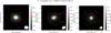 |
Fig. 2. Continuum-maps of IRC −10529. Low (left panel), medium (middle panel), and high (right panel) spatial resolution continuum map. Contours (in orange) are indicated in steps of (3, 6, 10, 100) |

– Channel maps: Figure 3 shows the low resolution channel map of 12CO J = 2 − 1 at 230.538 GHz and a lower state energy (Elow) of 5.53 K. We could not find any measurements with single antennas of the 12CO J = 2 − 1 v = 0 line in IRC-10529 in the literature, although there are such measurements for other sources in the ATOMIUM sample. Therefore to estimate the total amount of the CO flux recovered for this source, we referred to the observations of the J = 1 − 0 line with SEST (Nyman et al. 1992) and the J = 3 − 2 line observed with APEX-2a (De Beck et al. 2010), and to the Jy/K factors from the APEX/SEST web site15 and R. Laing (personal communication). We estimate an average flux density of ∼44 Jy for the J = 2 − 1 transition on the basis of a peak flux density of 16.2 Jy for the J = 1 − 0 line and 71 Jy for the J = 3 − 2 line, on the assumption that a flat-topped approximation to the profiles is adequate owing to the other uncertainties. ALMA recovered a peak flux density of 25 Jy for the J = 2 − 1 line, implying that we recovered > 55% of the most extended emission (and probably all the emission of the compact front and back caps). As discussed by Decin et al. (2020), the data show the prevalence of a broken spiral-like structure which can be explained by binary interaction caused by an as yet undetected (sub-)stellar companion. As an example of a medium-resolution channel map, we show the emission of the 111, 11 − 100, 10 transition of SO2 (at 221.965 GHz and Elow = 49.71 K), where the brightness distribution is composed of a hollow shell structure located at a radius of ∼2 5 (Fig. 4). A similar shell-like structure was previously seen for SO in oxygen-rich AGB stars with a high mass-loss rate by Danilovich et al. (2016), but the limitations of their data did not allow these authors to study the spatial distribution of SO2. The current ALMA data now confirm the emission of both SO and SO2 can have a shell-like structure, in accord with recent chemical model predictions (Van de Sande et al. 2018b; Danilovich et al. 2020b). The high-resolution channel map of the SiO J = 5 − 4 emission (at 217.105 GHz) is displayed in Fig. 5. Although the channel map is challenging to interpret at face value, the moment1-map has proven to be very valuable for understanding the velocity vector field in the inner wind region of various ATOMIUM sources (Decin et al. 2020), which (as shown in the next item) is illustrated very nicely in IRC−10529.
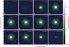 |
Fig. 3. Low resolution channel map of 12CO v = 0 J = 2 − 1 in IRC −10529. The peak of the continuum emission is at (0,0). The velocity (in km s−1) is with respect to the stellar velocity of −16.3 km s−1 (see the last column in Table 1), and is indicated in the upper right corner of each panel. The ALMA synthesized beam is shown as a white ellipse in the lower left corner of each panel (see Table E.2). The offsets in right ascension and declination are with respect to the peak of the continuum emission. |
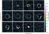 |
Fig. 4. Medium resolution channel map of SO2v = 0 11(1,11)−10(0,10) in IRC −10529. See Fig. 3 caption. The emission shows a hollow shell structure located at a radius of ∼2 |

– Moment1-map: First moment (or moment1) maps are utilised as a tool for visualising structures in the velocity fields. The maps are obtained by
 (1)
(1)
with the velocity channels centred around vLSR. We illustrate the strength of this visualisation for the low, medium, and high spatial resolution data of the SiO J = 5 − 4 emission of IRC −10529 (see Fig. 6). The line velocity map exhibits distinct red-shifted and blue-shifted components, which is the classical signature of rotation or a bipolar outflow (Kervella et al. 2016; Decin et al. 2020).
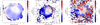 |
Fig. 6. SiO moment1-maps of IRC −10529. Low (left panel), medium (middle panel), and high (right panel) spatial resolution moment1-map of SiO v = 0 J = 5 − 4. The black cross indicates the position of the AGB star. The distinct spatial difference between red and blue-shifted velocity components indicates signs of rotation or bipolarity in the inner ∼0 |

– Spectra and line identifications: Shown in Figs. 7 and B.1–B.3 are the 16 spectral windows (spw) of IRC−10529 observed with medium resolution (mid configuration). The spectra were extracted with an aperture radius of 1 8 in the upper part of the panels and 0
 2 in the lower part, and are plotted on a common frequency scale. The line identifications shown in the upper panel were made using the spectral line catalogues of the Cologne Database for Molecular Spectroscopy (CDMS, Müller et al. 2001, 2005; Endres et al. 2016) and the Jet Propulsion Laboratory (JPL, Pickett et al. 1998), and by referring to prior spectral line surveys. In all, 60 lines from 12 molecules are observed in IRC−10529 in the mid configuration. These include CO, SiO, HCN, SO, SO2, SiS, CS, H2S, H2O, NaCl, KCl, and PO. Some molecular features, such as those of AlOH and OH (although not shown here), are only visible in the extended configuration, because the longer on-source observing time provides higher sensitivity to compact emission. In addition, there are a couple of weak features whose carriers have not yet been identified. The parameters of the molecular lines in IRC-10529 will be presented in the Molecular Inventory paper (Wallström et al., in prep., see Sect. 2.1.2).
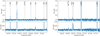 |
Fig. 7. Spectra of IRC−10529. Spectra of IRC −10529 for cubes 00 (left panel) and 01 (right panel) observed in the medium-resolution configuration with ALMA. The spectra were extracted with an aperture whose radius is 1 |


5. Result – Wind kinematics of the ATOMIUM AGB and RSG sources
5.1. Background
The ATOMIUM data introduced in Sect. 2.1 provides a unique opportunity for studying the wind kinematics in the circumstellar envelope of the 17 AGB and RSG sources. Here we use the data to understand where the wind is initiated, how fast it is accelerated, and if a terminal velocity is reached at some distance from the central star (Sect. 2.1.1). These questions can be answered by retrieving the wind velocity profile by analysing the extent of the emission from an ensemble of molecular transitions (for examples see Decin et al. 2015, 2018).
When the ALMA proposal was submitted, it was generally expected that most of the ATOMIUM sources, with the exception of W Aql, π1 Gru, and R Hya (Danilovich et al. 2015b; Feast 1953; Mason et al. 2001), were single stars. However, even for these three AGB sources, the known companion resides at a separation > 150 au so its gravitational field should not disturb the wind kinematics in the inner wind region (r ≲ 10 − 30 R⋆) where the wind is initiated. Hence, even for these three sources, the ATOMIUM data should allow us to study the efficiency of the wind initiation.
A first highlight of the ATOMIUM programme, however, was that no source displays a smooth spherical wind. Instead, the observed morphologies include bipolar geometries with a central waist, equatorial density enhancements (EDE) and disk-like geometries, spiral-like structures, arcs, and ‘eye’-like shapes. These morphologies, supported by a population synthesis approach, led to the conclusion that most ATOMIUM sources are part of a binary system, although the stellar or planetary properties and the orbital parameters of the companion remain unknown (Decin et al. 2020). It is expected that very-low-mass objects, including brown dwarfs and large planets, play a larger role than previously assumed. Therefore the ATOMIUM data renders a crucial observational benchmark for both binary-star and single-star theoretical simulations of the wind dynamics of AGB and RSG sources. Even though (sub-)stellar companions might be omnipresent, if the mass of the companion is low or the separation is large, there will be little departure of the velocity streaming lines from radial motion and the observed wind kinematics can guide single-star models. Moreover, even if a companion disturbs the radial velocity pattern substantially, the effect is ‘localised’ and the velocity pattern retains its radial character farther out in the wind. As discussed by El Mellah et al. (2020), any density structure imprinted in the wind will then expand in a self-similar way.
For the single-star and binary-star models, the question about the impact of resolved-out flux on the observables needs to be assessed. This mainly affects the low-excitation CO emission, however measurements of the velocity measure are not affected. Our observations are sensitive to MRS ≳8″ (Sect. 3.2.3), therefore all but the smoothest emission is detected. The perturbations and anomalous velocities we examine occur within 4″ of the star (as do the extreme velocities from a spherical shell). so resolved-out flux does not affect an investigation of the cause of perturbations. A next step entails assessing the mass fraction of the wind that is diverted for the binary-star models. To answer that question, single antenna observations are currently being acquired and analysed (Jeste et al., in prep.).
Single star models. It is generally accepted that the winds of AGB stars are radiation driven. Pulsations lift material to greater heights where the temperature is ≲1800 K, allowing gas to condense into grains (Hoyle & Wickramasinghe 1962; Gail & Sedlmayr 2013). The absorption of stellar radiation by these newly formed dust grains creates a net force that can overcome gravity (Höfner & Olofsson 2018). The gas is then accelerated beyond the escape velocity. This is expressed in the radial momentum transfer equation (Goldreich & Scoville 1976)
 (2)
(2)
where v(r) refers to the gas velocity at a radial distance r from the star, M⋆ the stellar mass, G the gravitional constant, and Γ(r) the ratio of the radiation pressure force on the dust to the gravitational force that can be written as (Decin et al. 2006)
![Mathematical equation: $$ \begin{aligned} \Gamma (r) = \frac{3 v(r)}{16 \pi \rho _s c G M_{\star } \dot{M}(r)}\int \!\!\!{\int {\frac{Q_\lambda (a,r) L_{\lambda } \dot{M}_d(a,r)}{a [{ v}(r)+{ v}_{\mathrm{drift}}(a,r)]}}} \,\mathrm{d}\lambda \,\mathrm{d}a \,, \end{aligned} $$](/articles/aa/full_html/2022/04/aa40431-21/aa40431-21-eq23.gif) (3)
(3)
with ρs the specific density of dust, c the speed of light, Ṁ the gas mass-loss rate, Ṁd the dust mass-loss rate, vdrift(a, r) the drift velocity of a grain of size a, Qλ(a) the dust extinction efficiency, Lλ the monochromatic stellar luminosity at wavelength λ. A solution for the gas velocity as derived from solving the momentum equation (Eq. (2)) for IK Tau is shown as the full black line in Fig. 8. If the grain properties change with radial distance so that, for example, Qλ(a, r) increases, a gradual wind acceleration at larger distances can arise (Chapman & Cohen 1986). In general, the particular behaviour of Qλ(a, r) has a strong influence on the wind acceleration, as discussed in detail by Netzer & Elitzur (1993).
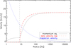 |
Fig. 8. Illustration of different velocity laws. The full black line at radii beyond 8 R⋆represents the solution of the momentum equation (Eq. (2)) derived for the wind velocity profile of the oxygen-rich AGB star IK Tau (Decin et al. 2010b); for the region between 1–8 R⋆ a beta-velocity law with β = 0.5 is used (Decin et al. 2006). The red dashed line illustrates the β-velocity law (Eq. (4)) for β = 0.5, v0 = 2.7 km s−1, v∞ = 17.68 km s−1, and the vertical black dashed line indicates Rdust at 8.6 R⋆. An almost perfect fit to the velocity as derived from the momentum equation (Eq. (2)) would be obtained for β = 1. The dotted blue line represents the Keplerian velocity law for material bound to a star of mass 1 M⊙. |
The wind initiation mechanism for RSG stars is less well understood. Mechanisms based on turbulent pressure in combination with radiation pressure on molecular lines or freshly synthesized dust grains and magneto-accoustic waves are invoked, or a combination of the above (Josselin & Plez 2007; Thirumalai & Heyl 2012). In general, these alternative processes might also support the AGB stellar wind, although their role in driving the wind is still very much debated (Wood 1990; Gustafsson & Höfner 2003). Solutions for the momentum equation (Eq. (2)) indicate that the velocity profile of AGB and RSG winds can be approximated by the so-called β-type velocity law (Lamers & Cassinelli 1999)
 (4)
(4)
with r the distance to the star, v0 the velocity at the dust condensation radius Rdust, and v∞ the terminal wind velocity (see red dashed line in Fig. 8).
The beta velocity law assumes that the CSE is physically homogenous, apart from a decrease in number density and temperature as a function of distance from the star. Low values for β describe a situation with a high wind acceleration. For carbon-rich AGB stars, β is around 0.5 (Decin et al. 2015) owing to the very opaque carbon dust grains that facilitate photon momentum transfer. Recent observational studies indicate that the wind acceleration for oxygen-rich AGB stars might be much lower than for carbon-stars, and values of β between 1 − 5 have been derived (Decin et al. 2010a, 2018; Khouri et al. 2014; Van de Sande et al. 2018a). The cause for this slow wind acceleration is not yet fully understood. The fact that oxygen-rich dust grains (such as aluminium oxides and silicates) are more transparent than carbon-rich grains offers part of the solution. Using colour-dependent absorption, it has been shown that silicates become progressively more iron-rich (hence opaque) as the material gets farther from the star (Woitke 2006; Bladh & Höfner 2012). However, even then we cannot explain why for some sources the observed wind acceleration continues beyond ∼50 stellar radii where the densities are too low for efficient momentum exchange between the gas and dust particles (see, for example, IK Tau in Fig. 9 of Decin et al. 2018). Fractal grains within an inhomogeneous clumpy wind increase the radiation pressure efficiency and can potentially explain the more gradual but ultimately more forceful acceleration (Decin et al. 2018).
Binary star models. As discussed in Decin et al. (2020), we expect that most of the ATOMIUM sources are part of a binary system. Binary interaction with a (sub-)stellar companion results in distinct non-spherical wind geometries that are readily probed in CO and SiO channel maps. Observationally derived wind profiles can provide a means for constraining the presence and the properties of a companion. Compared with a single-star model, the companion will perturb the radial character of the velocity vector field as expressed, for example, in the momentum equation (Eq. (2)) or in the β-velocity law (Eq. (4)). For example, in the case that the companion induces the formation of a Keplerian disk-like structure, the tangential velocity component is given by  , with G the gravitational constant, M⋆ the mass of the AGB star to which the disk is gravitationally bound, and r the radial distance (Kervella et al. 2016, see blue dotted line in Fig. 8). In addition, the companion’s gravity lowers the effective gravity felt by a particle driven from the primary AGB star, which can lead to a local enhancement of the velocity amplitude. Based on a 3D hydrodynamical simulation for a binary system containing a mass-losing AGB star (Fig. 9; El Mellah et al. 2020), we illustrate this effect in Fig. 10. In this simulation, the wind is initially accelerated from the primary star following a β-velocity profile with β = 5 (see black dashed curve in Fig. 10, illustrating the single-star model). The presence of the secondary object impacts the velocity profile; see dotted lines in Fig. 10. The first up/down peak in the radial velocity profile in the direction of the secondary (blue dotted line in Fig. 10) is due to the wind being first accelerated, but then dissipating most of its radial kinetic energy in the spiral shock, and having to be re-accelerated from scratch. To a lesser extent the same phenomena are apparent each time the radial ray crosses the spiral shock, hence the oscillating motion around the mean isotropic profile. Notice also that, as expected, the blue and red profiles oscillate with almost opposite phases. The isotropic velocity profile (black dotted line in Fig. 10) is then the average over all azimuthal and longitudinal angles of the velocity profile. In the example shown here, the isotropic velocity profile has a wave-like character, in which the first peak indicates the orbital separation and the higher harmonics are linked to the spiral-arm crossing. As we discuss below, the velocity profile of W Aql might be an example of the binary-induced effect described here.
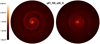 |
Fig. 9. 3D hydrodynamical simulation for a binary system containing a mass-losing AGB star. Slices of density are shown, in units of the density at the sonic point, in the orbital plane (left column) and in the plane containing the orbital axis and the line joining the two bodies (right column). The dimensionless parameters for this simulation are the mass ratio, q = M1/M2 = 1; the ratio of the terminal to orbital speed η = v∞/vorb = 2, the dust condensation radius filling factor f = Rd/RR, 1 = 20% (with RR, 1 the Roche lobe radius of the primary), and the β exponent setting the steepness of the velocity profile here being 5 (El Mellah et al. 2020). For a dust condensation radius set to 3 R⋆, the dimensionless parameters translate into an orbital separation of ∼35 R⋆. Due to binary interaction, a spiral shock is created in the circumstellar envelope. The spiral structure is readily recognised in the density slice in the orbital plane and the width of the successive spiral windings can be deduced from the density arcs in the edge-on view. |
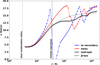 |
Fig. 10. Illustration of the impact of a binary companion on the velocity field. Given the simulations shown in Fig. 9 (El Mellah et al. 2020), the dotted black line represents the 1D isotropic radial velocity profile (w.r.t. the star). The dotted blue line is the radial velocity profile in the direction of the secondary, and the dotted red line is the radial velocity profile in the direction opposite to the secondary. For comparison, the dashed black curve illustrates the β-velocity law (Eq. (4)) for β = 5 representing the single-star situation. For better comparison with the observed velocity profiles (Sect. 5.2), the same figure but with a linear x-axis is shown in Fig. A.1. See text for more details. |
5.2. Methodology
To constrain the wind kinematics of the ATOMIUM sources, we followed the same methodology described in Decin et al. (2015) and Decin et al. (2018), which was augmented with several additional steps. Figures A.2–A.3 illustrate the methodology for the SiO J = 6 − 5 and NaCl J = 20 − 19 transition observed in the medium-resolution configuration of IRC −10529.
1. In the first step, the spectrum of each molecular transition was extracted for a range of circular apertures. The minimum diameter of the extraction aperture was the major axis of the synthesized beam (‘bmaj’, see Table E.3), the maximum diameter was the MRS (see Table E.3), where the step size was 2 × bmaj.
2. The velocity of the blue and red wings16 was determined for all extraction apertures. Accounting for the noise around the line spectrum (σline), the blue and red wing velocity were taken as the closest points to the line centre for which the flux was less than 3 × σline. These sensitivity-limited velocity widths are likely the lower bounds. The maximum of these numbers in absolute values was retained as the wind ‘velocity measure’ for the transition. The uncertainty in the velocity measure was taken from the spectral resolution of the data.
3. We then computed the zeroth moment map (integrated intensity or moment0 map) of each line (between the measured red and blue wing velocities) and measured the angular FWHM by fitting a 2D Gaussian profile to the moment 0 map using the Levenberg–Marquardt algorithm. If the least-squares minimisation was unsuccessful, the molecular transition was not retained for further analysis. This led to a significant reduction in the number of transitions retained for the analysis of the kinematical behaviour. This particularly affects transitions with low signal to noise ratios and/or high upper energy levels which are associated with having a small angular extent. Transitions whose moment 0 maps differ significantly from a 2D Gaussian profile – such as the SO2 distribution shown in Fig. 4 – were not retained after this step.
3. If the FWHM of the fitted 2D Gaussian was comparable to the axes of the synthesised beam (bmin, bmaj; see Table E.3), the non-deconvolved extent was taken as an upper limit to the distribution of the species. For transitions for which the FWHM of the fitted 2D Gaussian was larger than the synthesised beam, we deconvolved the beam. As in Decin et al. (2018), we assumed that the spatial FWHM of the molecular emission zone represents the dominant line formation region.
4. In the case of successful least-square minimization, the covariance matrix was used to estimate the variance of the FWHM (σFWHM). Accounting for the interferometric capabilities of ALMA, the total accuracy of the measured size of the emission is then given by
 (5)
(5)
where the S/N is the signal-to-noise ratio of the moment 0-map, θB the beamsize as given by (bmin, bmaj), and K is 0.5, 1, or 1.5 for the low, medium, and high spatial resolution data (Condon 1997; Taylor et al. 1999).
5. In the final step, the outcomes of the analysis of the velocity versus aperture information extracted from the low, medium, and high spatial resolution data were merged to produce a single output: for transitions in which the emission zone could be deconvolved in observations at various spatial resolution, the largest velocity measure and largest extent (often measured by the observation at the lowest spatial resolution) were retained. This should ensure that the impact of resolving out flux was kept to a minimum. In addition, blended lines were removed from the sample.
Our analysis provides a unique view of the wind kinematics of 17 oxygen-rich AGB and RSG sources. The outcome of this analysis for IRC −10529 is shown in Fig. 11, and that of the prototypical source W Aql is shown in Fig. 12. The wind dynamics for the 15 other sources are in Appendix C (see Figs. C.1–C.15). Until now similar velocity profiles were only obtained for the carbon-rich AGB star CW Leo (Ṁ = 1.5 × 10⁻⁵ M⊙ yr−1), and the two oxygen-rich AGB stars R Dor (Ṁ = 1 × 10⁻⁷ M⊙ yr−1) and IK Tau (Ṁ = 5 × 10⁻⁶ M⊙ yr−1) (Decin et al. 2015, 2018).
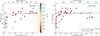 |
Fig. 11. Wind kinematics for IRC −10529. The wind velocities for all the molecular transitions observed in the low, medium, and high spatial resolution observations of IRC −10529 derived by the methodology described in Sect. 5.2. The velocities are plotted versus half of the spatial full-width-half-maximum (FWHM) of the molecular emission zone, and represent the dominant line formation region (Decin et al. 2018). The dotted blue vertical line indicates the radius at which the winds begin being accelerated (Rdust in Eq. (4); see Sect. 5.4), and the dotted black horizontal line is the velocity measure of the 12CO v = 0 J = 2 − 1 line. Only emission zones which could be spatially deconvolved are plotted (as dots) – the colour of the symbols are related to the energy of the lower state as indicated by the colour code bar. The grey cross on top of each coloured dot indicates the error bar in the derived velocity and in the FWHM, and is often smaller than the size of the dots. The error bars represent the fitting margin. Not accounted for here are the uncertainties due to the Gaussian approximation which might result in a systematic underestimate of the angular extent (see Sect. 5.2). The bottom axis is in units of arcseconds and the top axis is in units of the stellar radius. Left hand panel: zooms into the 150 stellar radii of the circumstellar envelope, and right hand panel: full extent of the detected wind emission. The 12CO v = 0 J = 2 − 1 transition (indicated in blue) only appears in the right hand panel owing to its large angular extent. The deconvolved data with a velocity less than that of the 12CO J = 2 − 1 transition, were fitted with a β-velocity law (Eq. (4)). Indicated in the legend in the right hand panel is β. The fit is represented by the full grey line which can be compared with a β-velocity law for β = 0.5 indicated by the red dashed line. |
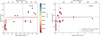 |
Fig. 12. Wind kinematics for W Aql. See Fig. 11 caption. The vertical blue dashed line at 0 |

One of the obvious limitations of the method is that we use Gaussian fits to the zeroth moment maps to determine the size of the emission zone. Inspection of individual channel maps and zeroth moment maps shows a variety of intensity distributions, depending on excitation effects, formation and depletion mechanisms, and the potential influence of a companion (see Sect. 5.4.2). In future work we will investigate different techniques such as fitting a modified power law (as in Sahai & Bieging 1993), an azimuthal average, or a cutoff such as 3 × σrms. These methods for determining the angular size are likely to strengthen the inference drawn from this analysis (see Sect. 5.4), because fewer transitions would be rejected owing to the lack of convergence of the Gaussian fitting method. We also will need to consider whether we are detecting essentially all the emission of each transition; or whether we are bounded by missing extended flux and/or sensitivity which varies between species. In general, the estimates of the maximum extent of any one transition might be biased if the CSE is not truly spherical, and depends on the orientation to the line of sight of any elongation.
Arguably, this is a simplified view of the wind kinematics since: (i) we only obtain a projected 1D view of the velocity vector field; and (ii) the spatial extents plotted in these figures might not always reflect the region where some of the extreme velocities arise from, for example in the situation where the extreme velocities are only reached at close distances from the AGB star while the bulk of the emission further out has lower velocities. Nevertheless, interesting conclusions can already be derived from these results (see Sect. 5.4).
5.3. Combining different angular resolution data and the issue of resolved-out flux
To date, there are two stars for which the three individual spatial resolution data and the combined dataset have been analysed in detail – π1 Gru (Homan et al. 2020) and R Hya (Homan et al. 2021) – thereby offering an opportunity to study the effect of resolved-out flux at a maximum recoverable scale for the lowest resolution ALMA ATOMIUM observations of ∼10″. Resolving out flux might be an issue for the measurement of the angular extent of the molecular emission, but this does not hinder the determination of the velocity measure, because resolving out flux mainly reduces the measured line flux of extended emission around the central velocities and not that of the line wings which represent the more compact front and back caps of the circumstellar envelope.
The combined data are significantly more sensitive to emission which has structure on sub-arcsec scales, than the individual configurations. For an angular resolution of between ∼0.1 and ∼8 arcsec, the combined data sets contain at least twice as much data as an individual configuration. The combined visibility data can be weighted as a function of baseline length to provide greater sensitivity for any desired resolution in this range, and this will be done in the detailed studies of each star. On smaller scales of tens of mas, the combined data set may also give a better image in the presence of extended structure although ’clean’ stability can then be an issue. The combined data therefore allows for a more accurate measure of the total extent of emission from some lines at intermediate distances from the star.
The three observing dates of the low, medium, and high spatial resolution data differ by up to ∼9 months, while AGB stars have typical pulsation periods of ∼0.5–2 yr (see Table 1; Cernicharo et al. 2014; Fonfría et al. 2018). Therefore, the higher-excitation molecular transitions which are excited close to the stellar surface, can vary between epochs, and while this may lead to a more complete picture in the combined data, extreme variability (e.g., SiO masers) causes artefacts that result in combined images which might not be reliable. For these lines, the velocity measurement is more accurate for the merged dataset (see Step 6 in Sect. 5.2) than for the combined dataset.
For some molecular transitions the Levenberg–Marquardt minimization used for fitting the 2D Gaussian profiles failed for the combined dataset, but was successful for (one of) the individual observations. An example is the 12CO J = 2 − 1 line where the emission zone in low spatial resolution data often better resembles a 2D Gaussian profile, but in the combined dataset the individual substructures are more prominent and a 2D Gaussian profile does not reproduce the observed emission. In general, an excellent correspondence is found for those molecular transitions that could be deconvolved in both the merged outcomes (of the low, medium, and high spatial resolution data; see Step 6 in Sect. 5.2) and the combined dataset. The differences between extents measured in the two ways have a dispersion of 0 06.
06.
Given these outcomes for π1 Gru, we have used the merged results from the datasets of individual spatial resolution for the study of the kinematics in all the ATOMIUM AGB and RSG envelopes.
The only question still remaining is whether some flux is resolved out beyond the ∼10″ scale. The two molecules most affected by resolved-out flux are CO and SiO, owing to their high abundance in these oxygen-rich sources, and hence potentially extended molecular envelopes. For each target, we have estimated the CO and SiO photodissocation region using the formula given by Mamon et al. (1988) and González Delgado et al. (2003), respectively (see Sect. 3.1). For all the ATOMIUM sources, the SiO emission zone – as estimated from the photodissociation radius following González Delgado et al. (2003) – is less than ∼3 5, with the exception of GY Aql where owing to its proximity to Earth the estimated SiO emission zone is ∼9″. Hence, resolving out flux should not be an issue for the SiO measurements. However, the CO emission zone for the ATOMIUM sources ranges between ∼20–300 ″, although the CO J = 2 − 1 transition is not excited up to the very outer boundary. This implies that the measured sizes of the 12CO and 13CO J = 2 − 1 transitions will be lower limits. This, however, does not hinder our present study on the wind kinematics, since we focus here on the wind initiation efficiency in the inner wind region, the maximum and minimum velocities deduced from the ATOMIUM data, and the imprint of a binary companion on the observationally derived wind velocity profiles. For all sources, additional observations of the 12CO J = 2 − 1 and 13CO J = 2 − 1 transitions have been or will be acquired with the APEX 12 m single antenna, allowing us to constrain the CO emission region with higher precision.
5.4. Interpretation
In this section, we aim for an interpretation of the observationally derived wind kinematic profiles displayed in Figs. 11, 12, and C.1–C.15. We first examine the wind acceleration in the ATOMIUM sources. As will be discussed, the majority of the ATOMIUM sources display a slow wind acceleration characterised by quite high values of β. However, the wind kinematic profiles also make it readily clear that the radial velocity description as provided by the momentum equation (Eq. (2)) or the β-velocity law (Eq. (4)) for single-star models cannot capture the complexity of the velocity field in the ATOMIUM sources. We therefore extend this discussion with a more detailed examination of some of the observationally derived velocity profiles in the context of binary-star models.
5.4.1. Single-star models: wind initiation and terminal wind velocities
The first theoretical studies discussing analytical approximations (Gehrz & Woolf 1971; Gilman 1972) and numerical solutions of the equation of motion (Kwok 1975; Goldreich & Scoville 1976), resulted in gas velocity profiles having a characteristic sharp rise and reaching a constant ‘terminal’ wind velocity, v∞, within the first few stellar radii (see also Fig. 8). Values for v∞ have been observationally derived from the half-line width of low-excitation rotational CO lines (see, for example, Loup et al. 1993). The predicted fast acceleration of the wind velocity also motivated various modellers to assume a constant wind velocity (for example, Ramstedt et al. 2009; Sargent et al. 2011; Groenewegen 2014). However, the ATOMIUM data show that the notion of a constant wind velocity being reached within ∼10 R⋆ is not consistent with the observations. For all ATOMIUM sources, large variations in the derived velocity measures are seen, even at radial distances greater than 50 R⋆, where (1D) spherical symmetric wind models with a steadily increasing velocity profile predict the velocity measure to have asymptotically reached the terminal wind velocity (see Fig. D.1).
In the approach adopted here we apply the same classical methodology in which a low excitation line of CO is used to determine the terminal wind velocity. However our approach differs from most earlier studies because: (1) it relies on a quantifiable metric linked to the 3σ rms noise in spectra that were observed at very high angular resolution and sensitivity; and (2) it does not rely on subjective judgement derived from visual inspection of less sensitive observations, or by referring to a model.
Various sources such as S Pav show some substantial changes in the velocity amplitude in the innermost few stellar radii. This behaviour might be reminiscent of pulsation-induced shocks for which hydrodynamical simulations show that they can lead to time-variable velocity characteristics within the first ∼4 stellar radii and with amplitudes of around 5–10 km s−1 (Bladh et al. 2019; Hoai et al. 2020, see Fig. D.3). The strongest effect is within the first 2 R⋆, but rapidly fades out at greater distances (Liljegren et al. 2018; Bladh et al. 2019). While the shock in the 3D hydrodynamical models is global in scale, the maximum velocity reached by the gas in the shock front is not uniform but rather clumpy. The medium and low-resolution data are less sensitive to compact emission, and hence the high-resolution and combined datasets should be used to diagnose this region that is disturbed by the shocks. Analogous to Khouri et al. (2016b); Khouri et al. (2019), we derive a first estimate of the velocity amplitude in this complex region from the high-resolution observations of the highly excited OH and CO v = 1 transitions. These data indicate velocities of around 6 – 10 km s−1. For three source (R Aql, R Hya, and S Pav) the OH and CO v = 1 transition both have an inverse P-Cygni profile which – in the framework of a 1D single-star model – can be interpreted as a sign of infall of material with velocities of around 10–15 km s−1. As discussed in Appendix D for the case of the ‘normal shock’ model, these shock characteristics cannot be traced in the medium and low-resolution data in the theoretical simulations of the 12CO v = 0 J = 2 − 1 and 28SiO v = 0 J = 5 − 4 line, and this is a conclusion which we extrapolate to the other molecular lines.
To compare our results here with the prior literature, we use the velocity retrieved from the ALMA CO v = 0 J = 2 − 1 line v(CO) to define the terminal wind velocity (v∞), and thereby assume CO traces the velocity of the bulk material at large distances from the star. To avoid potential impact from pulsation-induced shocks (see above and Appendix D), we opt to use the (low-resolution) data from the compact configuration ( (CO), see Col. 3 in Table 3).
Velocity parameters of the ATOMIUM sample.
As discussed in the Appendix D: (1) the effects of thermal and turbulent broadening in the wings of the line profile can be distinguished when CO is observed at high sensitivity; and (2) the low resolution CO data is indeed a good diagnostic for the terminal wind velocity. At a temperature of 2500 K, thermal broadening amounts to ∼1.2 km s−1. The turbulent broadening is difficult to estimate, but the example of De Beck et al. (2012) indicates a value of around 1.5 km s−1, so the combined effect yields a Gaussian broadening of the line wings with HWHM of around 2.2 km s−1. Excluding the fast, bipolar outflow traced in the 12CO J = 2-1 data of π1 Gru (see Sect. 5.4.2; Doan et al. 2017), the three red supergiants in the sample (AH Sco, KW Sgr, and VX Sgr) have the largest CO velocities. Even when we account for this broadening effect and for the spectral resolution of our ALMA data of ∼1.3 km s−1, the results in Table 3 still indicate higher terminal velocities than were derived previously for most ATOMIUM sources. With the exception of GY Aql, the compact configuration ATOMIUM data of CO yield a larger terminal wind velocity than previous values (see cols. 2 and 3 in Table 3), where the maximum difference is a factor of 2.1. The reason for this difference is the higher sensitivity of the ATOMIUM data which allows us to trace the broad CO wings whose intensity is low.
In their survey of 42 mostly southern AGB stars that includes 21 M-type stars, Ramstedt et al. (2020) observed the J = 2–1 line of 12CO in five of the ATOMIUM sources (T Mic, IRC–10529, IRC+10011, SV Aqr, and R Hya), but their observations were done with the ALMA 7 m Compact Array (ACA) – rather than with the ALMA 12 m Array which we used here. The synthesized beam of the ACA is about 5 arcsec and the 1σ rms of the data is about 40–110 mJy beam−1 in Band 6 (see Table B.1 in Ramstedt et al. 2020). When the ATOMIUM observations were made at low angular resolution in the compact configuration, the synthesized beam was about 7 times smaller (750 mas) and the 1σ rms (5 mJy beam−1) was about 15 times smaller than in Ramstedt et al. The method for determining the CO velocity measure in Ramstedt et al. and ATOMIUM are similar: (1) the CO line profile is extracted for a circular aperture, which in Ramstedt et al. consists of a fixed circular aperture of 18″ that is close to the maximum recoverable scale for these observations; and (2) the total velocity width (divided by a factor 2) is used to determine the CO velocity measure. Dividing the full width of the CO J = 2–1 line in Table B.1 of Ramstedt et al. by a factor of 2, the υmax(CO) is 6.25 km s−1 for T Mic, 15.25 km s−1 for IRC-10529, 19.5 km s−1 for IRC+10011, 9.4 km s−1 for SV Aqr, and 10.5 km s−1 for R Hya. Comparing these with  (CO) in Table 3, we find that
  (CO) determined in ATOMIUM is 1.5 − 2 times higher in four stars and 1.2 times higher in IRC+10011 than in Ramstedt et al. (2020) As illustrated in Fig. A.4, the 15 times higher sensitivity in the ATOMIUM observation of T Mic yields a much more sensitive diagnostic of the low level emission from the wings of the CO line profile and an estimation of υmax(CO).
Owing to resolved-out flux (see Sect. 5.3), in five out of the 17 sources a transition other than the 12CO J = 2 − 1 line has the largest apparent emission zone. In W Aql and GY Aql, the 13CO J = 2 − 1 line has a larger extent, while in IRC −10529 and IRC +10011 some transitions of SO2 probe larger regions. KW Sgr is in various ways an exception, because we have not acquired the low-resolution data and the 12CO J = 2 − 1 line remains undetected in the medium-resolution data – i.e., the data are sensitivity limited, owing to its large distance of 2 400 pc. Hence the CO extent plotted in Fig. C.12 is deduced from the high resolution data and some rotational transitions of SiO in the vibrational ground state which trace larger emission zones.
For all sources, except for π1 Gru, the value of υ(CO) is, however, lower than the velocity measure from other transitions with spatial emission zones lower than the extent of CO (see Cols. 4–6 in Table 3), implying the wind profile will never be captured by the solution of the momentum equation (Eq. (2)) and cannot be adequately reproduced using a β-velocity law. Nevertheless, we have tried to quantify approximately the region of the wind initiation and the wind acceleration efficiency by fitting the β-velocity law (Eq. (4)) to the data in which the velocity measure is lower than the velocity determined from the 12CO J = 2 − 1 line. The fits account for the variance on the measure of the velocity, and the emission extent. Equation (4) has three free parameters (v0, Rdust, and β). The parameters v0 and Rdust are not straightforward to quantify, because of the pulsation-induced shocks (see above). We therefore empirically estimate these two parameters17.
To be a reliable measure of the velocity, the line profile should encompass at least three spectral resolution elements. Given the spectral resolution of ∼1.3 km s−1, this results in the minimum measurable velocity of around 4 km s−1 (as can be seen in Col. 7 of Table 3). Often the corresponding transitions are high-excitation transitions (see Col. 8 in Table 3), although in some cases the lowest velocity measure is derived for weak, low-excitation transitions with restricted signal-to-noise ratios. The parameter v0 is determined as the minimum of the derived velocity measures (for both non-deconvolved and deconvolved emission; see Step 4 in Sect. 5.2), but should be larger than the local sound speed of ∼4 – 5 km s−1.
The parameter Rdust is then quantified as the radius at which v0 is reached, but should be larger than 2 R⋆. The derived values of Rdust vary between 2–6.7 R⋆(see Table 3). We caution against over interpreting Rdust as the radius where the dust formation is starting, owing to the unknown effects of pulsation-induced shocks.
Using a Levenberg–Marquardt minimization routine, β is derived with its variance as given by the covariance matrix (see last two columns in Table 3) and – as can be seen in Table 3 – β varies between 0.6–9.1. In four sources (U Del, V PsA, SV Aqr, and KW Sgr) not enough data points with v < v(CO) are available to determine β (see Figs. C.3–C.5, and C.12). For sources with Ṁ ≳ 5 × 10⁻⁷ M⊙ yr−1 in which the spatial emission zone of a significant fraction of the molecular transitions could be deconvolved, we often see that the wind acceleration continues up to ∼100 R⋆ and is represented by high values of β. Some examples include RW Sco, AH Sco and GY Aql.
The ATOMIUM data provides some insight into the wind initiation efficiency, particularly on the frequently observed low wind acceleration. But Figs. 11, 12, and C.1–C.15 confirm that the velocity vector field for all the ATOMIUM sources is more complex than is captured by current 1D hydrodynamical models. Pulsation-induced shocks can explain some of the velocity variation in the innermost few stellar radii, but as discussed in the next section this scenario cannot explain the complex kinematic behaviour seen in most ATOMIUM sources.
5.4.2. ATOMIUM wind profiles interpreted within the context of binary-star models
Two conclusions can be drawn from the plots of the wind kinematics: (1) the velocity measures in Table 4 which were derived from different rotational transitions and from different molecules at the same distance from the star (see Cols. 6 and 8 in Table 3), differ by more than the 3σ of the velocity resolution; and (2) the differences in the velocity measures correspond to real anomalies in the behaviour of the species. The wind kinematic plots also show that the SiO velocities are greater than than those of CO in 15 of the 17 ATOMIUM sources (i.e., all sources except π1 Gru and RW Sco) by up to a factor ∼1.6, and in six sources the velocity measure derived from other molecular lines are also greater than that of CO (see Tables 3–4). However, CO has a larger extent than SiO for all sources except KW Sgr (see Fig. D.2, and Sect. 5.4.1). In general, the CO emission is expected to extend roughly an order of magnitude farther than the SiO emission (see Sect. 5.3). The low-excitation CO line is predominantly collisionally excited, and is a reliable tracer of the density in the outer wind region. The Einstein A coefficients of the rotational lines of SiO in the ground-vibrational state are three orders of magnitude higher than those of CO, and as a result the rotational lines of SiO are sensitive to radiative (de-)excitation effects implying that these lines are key diagnostics for tracing the complex kinematics in the inner wind regions.
Velocity measures of SiO versus CO.
Given our current physical understanding, pulsation-induced shocks are not a viable mechanism to explain the wind kinematic profiles of most of the ATOMIUM sources, in particular for the case where larger SiO velocities are traced in the compact and medium configuration data (see the Appendix D). Hence other mechanisms should be considered. An obvious candidate is binary interaction – see our results published in Decin et al. (2020). Simulations for binary systems with a mass-losing AGB star as primary indicate that circumbinary disks are dynamically formed for systems with orbital separation ≲6 au and mass-ratios in the order of 0.5–1 (Chen et al. 2017). A Keplerian (or in general rotational) velocity field (see dotted blue line in Fig. 8) can lead to velocities projected along the line-of-sight in excess of the terminal velocity in the innermost few stellar radii; see for example the case of L2 Pup (Kervella et al. 2016). However, such a disk cannot explain the high velocity indicated for most sources in the centre and right hand columns of Table 4, which show high velocity SiO emission extends by more than ∼30 R⋆ (in diameter). We propose here that the gravitational influence of the binary companion (residing at a wide separation) is the cause for the latter behaviour, in particular for those sources in the last column of Table 4 for which various molecules trace large velocities. For example, if there is a (binary-induced) density contrast between an equatorial density enhancement and a biconical outflow or lobes, the velocities in these directions might differ, and they might not always favour the lobes if a denser equatorial region is more efficiently dust driven. As the result, the density differential will favour different species in the kinematical plots which are at the same distance from the star, but which have different velocities.
Checking the low-, medium-, and high-resolution data of the high-velocity lines, it becomes clear that in most cases the highest velocity value is observed in the high resolution data. This points towards excess high velocity emission arising from the shocked inner wind region, often within ∼2–10 R⋆ (Cernicharo et al. 1997; Herpin et al. 1998; Vlemmings et al. 2017, see the Appendix D). For the binary hypothesis to hold in the situation of a separation above ∼10 stellar radii, we need to know if there is high velocity emission at other locations in the wind farther away from the central star, which we refer to here as the persistence test. We therefore check if high velocity emission (from molecules other than CO) can be detected in the low and medium resolution data. Because the lower resolution data were observed for a shorter time, they are less sensitive to compact emission. If the emission only arises from the innermost few stellar radii, no maximum radius or Gaussian fit can be determined from the lower resolution data following the procedure outlined in Sect. 5.2, and we then categorise the emission as non-persistent. The persistence test reaches two levels: level 1 applies to the sources in the second column of Table 4, in which only SiO transitions reach velocities above the one deduced from the CO v = 0 J = 2 − 1 line; level 2 applies to sources in the last column of Table 4, in which molecules other than SiO also reach velocities above CO. The persistence test fails for five sources (U Del, V PsA, U Her, R Aql, and KW Sgr), but is successful for four sources at level 1 (S Pav, T Mic, SV Aqr, and R Hya), and six sources at level 2 (AH Sco, W Aql, GY Aql, IRC −10529, IRC +10011, and VX Sgr). Obviously, all targets in the last column of Table 4 pass, which is not unexpected given the argument that molecules other than SiO are also diagnostics for the binary hypothesis. Hence, for the ten sources that pass the persistence test at either level 1 or level 2, we investigated whether we could deduce an approximate orbital separation from the kinematic information in Figs. 11, 12, C.1, C.2, C.5, C.6, C.9, C.11, C.13 and C.14.
W Aql was first identified as a spectroscopic binary by Herbig (1965). Ramstedt et al. (2011) used Hubble Space Telescope (HST) data, with a spatial resolution of 0 12, to deduce the projected separation of 0
 46 (∼150 au or ∼85 R⋆). The inclination of the orbit is unknown, and therefore the orientation of both sources relative to each other could not be deduced from these data, although Danilovich et al. (2015b) finds that the F8-G0 companion, with mass around 1 M⊙, cannot be in front of the AGB star.
We note that a close companion can increase the terminal wind velocity as compared to a single star model owing to the slingshot mechanism (Maes et al. 2021). Morever as illustrated in Fig. 10, the gravitational attraction by a binary companion can induce an increase in the velocity amplitude at radii smaller than the orbital separation, eventually leading to a wave-like velocity profile beyond the orbital separation. These predictions are roughly consistent with the velocity profile of W Aql derived from the ATOMIUM data in Fig. 12, in which around 80 R⋆we see both an increase and a decrease of the velocity measures with respect to the beta law. However the observed pattern is not as sharp as in the theoretical simulation in Fig. 10 (see also Fig. A.1) because: (1) the observations correspond to projected velocities; and (2) the binary system in W Aql might be more complex than the simulations. Given this first-order agreement, we use the closest location beyond 10 R⋆ where the velocity gradient turns negative as a proxy for a tentative indication of the upper limit on the orbital separation for those sources that pass the persistence test. Admittedly, this is not deduced straightforwardly for all sources. For those cases in which there are only a few points to guide us in this exercise, we have opted to list the extent of the molecule with the highest velocity measure (vmax) which for W Aql would yield 0 69 (or 125 R⋆). This difference between the first estimate of ∼80 R⋆ – as deduced from the negative gradient of the velocity pattern, and ∼125 R⋆ as retrieved from vmax – also marks the limitations of the method proposed here for estimating the orbital separation.
Two other ATOMIUM sources in addition to W Aql are confirmed binaries (R Hya and π1Gru). The companion of R Hya is thought to have a very wide orbital separation of 21″ (Mason et al. 2001) which is beyond the field of view of the ATOMIUM data. In R Hya there is also evidence of dramatic perturbations in the CSE within a few 100R⋆ of the central star, possibly owing to a second companion (Homan et al. 2021). π1Gru has a companion of spectral type G0V at a separation of 2 7 (∼500 au, Feast 1953), but there is no signature of the known companion in the line or continuum data of ATOMIUM.
Following a similar approach as for W Aql in Fig. 12, we derived an orbital separation for IRC–10529 from the velocity profile in Fig. 11, and the orbital separations for the eight other stars that pass the persistence test from the velocity profiles in Appendix C of: 0.20″ − 0.30″ for S Pav, T Mic, SV Aqr, GY Aql, and IRC+10011; and between 0.45″ − 1.00″ for AH Sco, R Hya, and VX Sgr.
In π1Gru, the width of the 12CO J = 2 − 1 line is more than a factor of 2 larger than that of any other molecular transition. The large line width – which had also been seen in previous ALMA 12CO J = 3 − 2 data – was interpreted as an indication that the envelope structure of π1 Gru includes a radially expanding equatorial torus (with a velocity of 8–13 km s−1); and a fast bipolar outflow (with a linear velocity increase from 14 km s−1 at the base up to 100 km s−1 at the tip), with an angle between the line of sight and the equatorial plane of 40° (Doan et al. 2017). However, a spiral pattern has emerged in more recent higher spatial resolution ALMA 12CO J = 3 − 2 data, and the spiral-arm separation hints towards the presence of a companion with a separation of less than 70 AU (or 34 R⋆; Doan et al. 2020). The ATOMIUM data will now further refine this picture, since various other molecules have line wings up to ∼40 km s−1 and exhibit clear signs of rotation or bipolarity in their moment 1 maps – see for example the SiO J = 5 − 4 and J = 6 − 5 lines in Homan et al. (2020). The separation between the arc-like structures observed in the ATOMIUM12CO J = 2 − 1 channel maps (Decin et al. 2020), indicates the presence of a second companion with an orbital separation of around 0 04; and the dynamics traced by the SiO masers, suggest a (tentative) upper limit of the companion mass of ∼1.1 M⊙ (Homan et al. 2020, Montargès et al., in prep.).
5.5. Discussion and implications
Putting these results in the context of the overall goals of the ATOMIUM project, it is clear that important science questions posed in Sect. 2.1.1 can be addressed by the ATOMIUM data. The wind acceleration efficiency, as expressed by the quite large values of β, seems quite low in general. The slow wind acceleration in turn yields constraints on the composition, size, and formation radius of dust grains, expressed for a single-star model by the dust extinction efficiency Qλ(a, r) in Eqs. (2) and (3). In addition, the question of the enforced wind dynamics in the intermediate wind region needs to be reformulated and should incorporate a search for the impact of binary companions on the wind dynamics of AGB and RSG stars.
Within both a single-star and a binary-star context, the results derived here have an impact on our understanding of the mass-loss rate for the following two reasons:
(i) When comparing prior results to those obtained in the ATOMIUM project, the velocities v(CO) derived from the low excitation line of 12CO J = 2 − 1 are systematically higher when derived from the ATOMIUM data. Since v(CO) is often used as a measure for the terminal wind velocity in single-star models, a direct implication is that the mass-loss rate for these sources will be underestimated. The high sensitivity of the current ALMA data was the key for deriving these higher wind velocities. As noted in Sect. 5.4.1, under the condition of single star models the larger CO velocities might imply larger terminal velocities and larger values of Ṁ, because the random scatter from the thermal line broadening and turbulence cannot explain these large velocities. As a result, we surmise that the terminal wind velocities and hence gas mass-loss rates will be underestimated for other AGB and RSG sources as well.
It might also be the case that the higher CO velocities (and those of other molecules) indicate exceptional motions owing to binary interaction. Under the condition of binary companions, the larger CO velocities might not be an indication of larger terminal velocities of the bulk material, but we are currently unable to estimate the relative effect in the single versus binary model, because assessing the impact of the companion on the Lagrangian (see Gregory 2006) would require extensive hydrodynamical simulations.
(ii) The current results support the conclusion in Decin et al. (2020) that (sub-)stellar binary interaction is the prime wind shaping agent of the majority of AGB/RSG stars, including the ATOMIUM sources whose mass-loss rates exceed the nuclear burning rate of around 1 × 10⁻⁷ M⊙ yr−1. In the majority of the ATOMIUM sources, molecular transitions other than the 12CO v = 0 J = 2 − 1 line trace a larger velocity amplitude than CO, and have a spatial emission zone that is often greater than 30 stellar radii, but is much less than the extent of CO. This result has a two-fold repercussion on our historical insight of mass-loss rates in AGB and RSG which were derived within the context of single-star models:
-
For close binary systems, a massive planet or stellar companion can enhance the AGB/RSG mass-loss rate by depositing angular momentum into the envelope and by reducing the effective gravity of the mass-losing star. Single stars or binary stars isolated from angular momentum deposition hence might suffer from a lower mass-loss rate during the AGB/RSG phase than stars prone to angular momentum deposition (Sabach & Soker 2018). Hydro-chemical simulations stimulated by the results of the ATOMIUM survey, indicate this difference might be up to almost an order of magnitude (Bolte et al., in prep., Decin 2021).
-
There are profound implications for the classical measures of the AGB/RSG mass-loss rate derived under the assumption of a single star with a spherical wind. For a mass-losing AGB/RSG star in a binary system, the material flow will have a directional preference towards the orbital plane; and spiral arcs, circumbinary and accretion disks, etc. can be created (see, for example Mastrodemos & Morris 1999; Mohamed & Podsiadlowski 2012; Kim & Taam 2012; Liu et al. 2017; Chen et al. 2017; Saladino et al. 2019; El Mellah et al. 2020). As such, previous mass-loss rate estimates based on the assumption of spherical symmetry should be interpreted with care since systematic errors might occur, as shown recently by Homan et al. (2015, 2016), and Decin et al. (2019). We conjecture that in general, mass-loss rates hitherto derived from dust spectral features will be systematically overestimated. This conjecture is based on the fact that the companion’s gravitational attraction can create an equatorial density enhancement (EDE) with a density contrast that can be up to an order of magnitude higher than the background wind density (El Mellah et al. 2020). The spectral energy distribution (SED) in the near- and mid-infrared mainly traces warm dust residing close to the star, hence in the EDE. Therefore, depending on the inclination of the EDE, the analysis of dust spectral features using a simplified 1D approach reflects the higher density in the EDE created by the binary interaction, but not the actual mass-loss rate which will be lower. This conjecture is in line with previous observations which indicated that mass-loss rates derived from dust features are about an order of magnitude larger than mass-loss rates from CO observations (e.g., Heske et al. 1990).
These implications have a profound impact on several aspects of stellar evolution. Because the mass is the prime parameter determining the evolution and lifetime of a star, any modification to the stellar mass-loss over time has large repercussions on its evolutionary path.
If we would only account for (i), then a higher mass-loss rate implies a shortening of the AGB (RSG) phase. However, recent studies indicate that most stars in the universe will have one or more stellar or gas-giant planetary mass companions (Moe & Di Stefano 2017; Nielsen et al. 2019; Fulton & Petigura 2018; Fulton et al. 2019). Hence, most empirically derived mass-loss rates are from samples containing a large fraction of stars that experience binary interaction with a (sub-)stellar companion. As such, our knowledge of the mass-loss rate will be biased by the impact that companions can have both on the magnitude of the mass-loss and on the observed diagnostics from which mass-loss rates are retrieved. Given (ii) implies that the mass-loss rate for these cool evolved stars can be seriously overestimated in current stellar evolution models for single stars. These models use mass-loss rate prescriptions to calculate the change of mass during the AGB and RSG phase, whose parametric relations for the mass-loss rate are often based on fitting infrared colours or the dusty SEDs (Reimers 1975; de Jager et al. 1988; van Loon et al. 1999, 2005). The impact of the effects discussed in (ii) are somewhat countered by the increase in mass-loss rate prescribed by (i), but the amplitude of the effect discussed in (i) is lower than those in (ii). The white-dwarf initial-final mass function (see for example Cummings et al. 2018) limits the total mass-loss occurring during the AGB phase. Hence, this result implies that the AGB phase will be longer for single stars. For single stars with initial mass greater than ∼8 M⊙, the mass before exploding as supernovae will be higher implying a larger fraction of more massive neutron stars can form. In addition, this implies that the contribution of cool evolved stars to the (extra)galactic dust budget will be lower than currently stipulated (see for example Matsuura et al. 2009, 2013), and the issue of the ‘missing dust-mass problem18’ is far from solved (Matsuura et al. 2009)
Dust-to-gas mass ratios for M-type AGB stars retrieved empirically are on average 5.8 × 10⁻³, while for carbon and S-type AGB stars they are around 2.5 × 10⁻³ and 2.8 × 10⁻³, respectively (Groenewegen & de Jong 1998; Groenewegen et al. 1999; Ramstedt et al. 2008, 2009; Danilovich et al. 2015a). Combining (i) and (ii) implies the dust-to-gas mass ratio for these samples, with derived gas mass-loss rates ≲1 × 10⁻⁵ M⊙ yr−1 for the carbon and S-type AGB stars and ≲7 × 10⁻⁵ M⊙ yr−1 for the M-type AGB stars, will be lower than current empirically derived values indicate. This conclusion impacts all studies that are (or have been) using a dust-to-gas mass ratio to compute total mass-loss rates from retrieved dust masses for which most often the canonical dust-to-gas ratio of 1/200 (as derived from galactic ISM studies) is used (see for example Matsuura et al. 2009, 2013).
ATOMIUM: ALMA Tracing the Origins of Molecules In dUst-forming oxygen-rich M-type stars; https://fys.kuleuven.be/ster/research-projects/aerosol/atomium/atomium. The ATOMIUM proposal was selected as a Large Programme in Cycle 6 with 113.2 h allotted (2018.1.00659.L, PI L. Decin), and is the first ALMA Large Programme in the field of ‘Stellar Evolution’.
The term ‘correlated density structures’ refer to arcs, spirals, disks, bipolar structures, shells, etc. ‘Uncorrelated density structures’ refer to clump-like morphologies which do not appear to be correlated with any other morphology.
Hereafter, all rotational transitions are in the ground (v = 0) vibrational state unless otherwise specified.
While this paper was in the final stage of preparation, the Gaia Early Data Release 3 (Gaia EDR3) became available. In 12 out of 15 ATOMIUM stars the distances in Gaia EDR3 are within ∼20% of the distances we have used here (see Table 1); two objects have no Gaia measurements (IRC–10529 and IRC+10011); and two of the remaining three stars have maser parallax distances that should be more accurate. We have adopted the distance for W Aql from Gaia EDR3 which is consistent with that in Danilovich et al. (2021); and the maser parallax distance for AH Sco of 2260 pc (Chen & Shen 2008), which is closer (by 21%) than the Gaia DR2 distance. Although the maser parallax distance for VX Sgr that we have adopted is at odds with Gaia EDR3, it is consistent with all previous measurements including Gaia DR2 (Richichi et al. 2005; Paladini et al. 2018).
See the ALMA Cycle 6 Technical Handbook at https://almascience.nrao.edu/documents-and-tools/cycle6/alma-technical-handbook.
‘Flagging’ is a term used in radio astronomy which refers to the process of identifying faulty or questionable portions of data that are not used in further steps of the data analysis and imaging.
For announcements and links to products see: https://fys.kuleuven.be/ster/research-projects/aerosol/atomium/atomium.
Many OH/IR stars were first observed in the two micron Caltech (IRC) sky survey (Neugebauer & Leighton 1969), and were subsequently shown by radio astronomers to have intense lines from OH and H2O masers. Most of the stars in the IRC catalog are M-type stars which have high mass-loss rates.
Negative velocities (i.e., blue shifted) with respect to the vLSR represent material coming towards the observer, and positive velocities (i.e., red shifted) with respect to the vLSR represent material receding from the observer.
The acceleration of the gas and dust begins at R0, however – consistent with the prior work by Maercker et al.; Decin et al. (2016; 2018, and references therein) – we do not distinguish between Rdust and R0 here, because the difference between Rdust and R0 of ≲10 R⋆ is small compared with the large scale description of the wind velocities that extend up to about 100 − 200 R⋆ in many of the ATOMIUM stars.
The missing dust-mass problem refers to the Large Magellanic Cloud and other high-z galaxies whose accumulated dust mass from AGB and RSG stars (and possibly supernovae) over the dust lifetime is significantly less than the dust mass in the ISM.
Acknowledgments
The authors are grateful to a referee for the close reading of the manuscript and the constructive comments. This paper makes use of the following ALMA data: ADS/JAO.ALMA#2018.1.00659.L, ‘ATOMIUM: ALMA tracing the origins of molecules forming dust in oxygen-rich M-type stars’. ALMA is a partnership of ESO (representing its member states), NSF (USA) and NINS (Japan), together with NRC (Canada) and NSC and ASIAA (Taiwan), in cooperation with the Republic of Chile. The Joint ALMA Observatory is operated by ESO, AUI/NRAO and NAOJ. This paper makes use of the CASA data reduction package: https://casa.nrao.edu/ (McMullin et al. 2007). - Credit: International consortium of scientists based at the National Radio Astronomical Observatory (NRAO), the European Southern Observatory (ESO), the National Astronomical Observatory of Japan (NAOJ), the CSIRO Australia Telescope National Facility (CSIRO/ATNF), and the Netherlands Institute for Radio Astronomy (ASTRON) under the guidance of NRAO. The National Radio Astronomy Observatory is a facility of the National Science Foundation operated under cooperative agreement by Associated Universities, Inc. The authors thank the Quality Assurance team at ESO for customising the imaging pipeline. We thank IRIS for provision of high-performance computing facilities. STFC IRIS is investing in the UK’s Radio and mm/sub-mm Interferometry Services in order to improve the data quality and allow much more data to be processed. This paper makes use of the Cologne Database for Molecular Spectroscopy (CDMS; https://cdms.astro.uni-koeln.de/classic/) and the spectral line catalogs of the Jet Propulsion Laboratory (JPL, https://spec.jpl.nasa.gov); Funding: We acknowledge travel support for consortium meetings from the RadioNet MARCUs programme under the European Community Framework Programme 7, Advanced Radio Astronomy in Europe, grant agreement no.: 227290, L.D., D.G., W.H., J.B., J.M.C.P., and S.H.J.W. acknowledge support from the ERC consolidator grant 646758 AEROSOL, L.D. and E.C. acknowledge support from the KU Leuven under the C1 MAESTRO grant C16/17/007, W.H. acknowledges support from the FWO Flemish Fund of Scientific Research under grant G086217N, F.H. acknowledges support from the “Programme National de Physique Stellaire” (PNPS) of CNRS/INSU co-funded by CEA and CNES, J.M.C.P. acknowledges support from the UK STFC grant ST/P00041X/1, J.Y. acknowledges support from the UK STFC grant ST/R001049/1, M.V.d.S. acknowledges support from the FWO through grant 12X6419N, T.D. acknowledges support from the FWO through grants 12N9917N and 12N9920N, A.B. acknowledges support from the “Programme National de Physique Stellaire” (PNPS), I.M. acknowledges funding by the UK STFC grant ST/P000649/1, E.D.B. acknowledges financial support from the Swedish National Space Agency, I.E.M. acknowledges support from the FWO and the European Union’s Horizon 2020 research and innovation program under the Marie Skłodowska-Curie grant agreement No 665501, S.E. acknowledges funding from the UK STFC as part of the consolidated grant ST/P000649/1 to the Jodrell Bank Centre for Astrophysics at the University of Manchester, P.K. acknowledges support from the French PNPS of CNRS/INSU, C.A.G. acknowledges support from NSF grant AST-1615847, T.J.M. is grateful to the STFC for support under grant ST/P000312/1, A.A.Z. was supported by the STFC under grants ST/T000414/1 and ST/P000649/1, M.D.G. thanks the STFC for support under consolidated grant ST/P000649/1 to the JBCA.
References
- Adam, C., & Ohnaka, K. 2019, A&A, 628, A132 [NASA ADS] [CrossRef] [EDP Sciences] [Google Scholar]
- Agúndez, M., Cernicharo, J., & Guélin, M. 2010, ApJ, 724, L133 [CrossRef] [Google Scholar]
- Agúndez, M., Cernicharo, J., Quintana-Lacaci, G., et al. 2017, A&A, 601, A4 [Google Scholar]
- Agúndez, M., Martínez, J. I., de Andres, P. L., Cernicharo, J., & Martín-Gago, J. A. 2020, A&A, 637, A59 [Google Scholar]
- Alma, P., Fomalont, E. B., Vlahakis, C., et al. 2015, ApJ, 808, L1 [NASA ADS] [CrossRef] [Google Scholar]
- Andronov, I. L., & Chinarova, L. L. 2012, Odessa Astron. Publ., 25, 148 [Google Scholar]
- Arroyo-Torres, B., Wittkowski, M., Marcaide, J. M., & Hauschildt, P. H. 2013, A&A, 554, A76 [NASA ADS] [CrossRef] [EDP Sciences] [Google Scholar]
- Bailer-Jones, C. A. L., Rybizki, J., Fouesneau, M., Demleitner, M., & Andrae, R. 2021, AJ, 161, 147 [Google Scholar]
- Bennett, P. D. 2010, ASP Conf. Ser., 425, 181 [NASA ADS] [Google Scholar]
- Bertschinger, E., & Chevalier, R. A. 1985, ApJ, 299, 167 [NASA ADS] [CrossRef] [Google Scholar]
- Bladh, S., & Höfner, S. 2012, A&A, 546, A76 [NASA ADS] [CrossRef] [EDP Sciences] [Google Scholar]
- Bladh, S., Liljegren, S., Höfner, S., Aringer, B., & Marigo, P. 2019, A&A, 626, A100 [NASA ADS] [CrossRef] [EDP Sciences] [Google Scholar]
- Boulangier, J., Gobrecht, D., Decin, L., de Koter, A., & Yates, J. 2019, MNRAS, 489, 4890 [CrossRef] [Google Scholar]
- Bowen, G. H. 1988, ApJ, 329, 299 [NASA ADS] [CrossRef] [Google Scholar]
- Bromley, S. T., Gómez Martín, J. C., & Plane, J. M. C. 2016, Phys. Chem. Chem. Phys. (Incorporating Faraday Trans.), 18, 26913 [NASA ADS] [CrossRef] [Google Scholar]
- Bujarrabal, V., Fuente, A., & Omont, A. 1994, A&A, 285, 247 [NASA ADS] [Google Scholar]
- Bujarrabal, V., Alcolea, J., Mikołajewska, J., Castro-Carrizo, A., & Ramstedt, S. 2018, A&A, 616, L3 [NASA ADS] [CrossRef] [EDP Sciences] [Google Scholar]
- Castro-Carrizo, A., Quintana-Lacaci, G., Neri, R., et al. 2010, A&A, 523, A59 [NASA ADS] [CrossRef] [EDP Sciences] [Google Scholar]
- Cernicharo, J., Alcolea, J., Baudry, A., & Gonzalez-Alfonso, E. 1997, A&A, 319, 607 [Google Scholar]
- Cernicharo, J., Teyssier, D., Quintana-Lacaci, G., et al. 2014, ApJ, 796, L21 [NASA ADS] [CrossRef] [Google Scholar]
- Cernicharo, J., Marcelino, N., Agúndez, M., & Guélin, M. 2015, A&A, 575, A91 [NASA ADS] [CrossRef] [EDP Sciences] [Google Scholar]
- Chapman, J. M., & Cohen, R. J. 1986, MNRAS, 220, 513 [NASA ADS] [Google Scholar]
- Chen, X., & Shen, Z. Q. 2008, in The Art of Modeling Stars in the 21st Century, eds. L. Deng, & K. L. Chan, 247 [Google Scholar]
- Chen, X., Shen, Z.-Q., & Xu, Y. 2007, Chin. J. Astron. Astrofis., 7, 531 [NASA ADS] [CrossRef] [Google Scholar]
- Chen, Z., Frank, A., Blackman, E. G., Nordhaus, J., & Carroll-Nellenback, J. 2017, MNRAS, 468, 4465 [NASA ADS] [CrossRef] [Google Scholar]
- Cherchneff, I. 2006, A&A, 456, 1001 [NASA ADS] [CrossRef] [EDP Sciences] [Google Scholar]
- Cherchneff, I. 2011, A&A, 526, L11 [NASA ADS] [CrossRef] [EDP Sciences] [Google Scholar]
- Chiavassa, A., Lacour, S., Millour, F., et al. 2010, A&A, 511, A51 [NASA ADS] [CrossRef] [EDP Sciences] [Google Scholar]
- Condon, J. J. 1997, PASP, 109, 166 [NASA ADS] [CrossRef] [Google Scholar]
- Cummings, J. D., Kalirai, J. S., Tremblay, P. E., Ramirez-Ruiz, E., & Choi, J. 2018, ApJ, 866, 21 [NASA ADS] [CrossRef] [Google Scholar]
- Danilovich, T., Bergman, P., Justtanont, K., et al. 2014, A&A, 569, A76 [NASA ADS] [CrossRef] [EDP Sciences] [Google Scholar]
- Danilovich, T., Teyssier, D., Justtanont, K., et al. 2015a, A&A, 581, A60 [NASA ADS] [CrossRef] [EDP Sciences] [Google Scholar]
- Danilovich, T., Olofsson, G., Black, J. H., Justtanont, K., & Olofsson, H. 2015b, A&A, 574, A23 [NASA ADS] [CrossRef] [EDP Sciences] [Google Scholar]
- Danilovich, T., De Beck, E., Black, J. H., Olofsson, H., & Justtanont, K. 2016, A&A, 588, A119 [NASA ADS] [CrossRef] [EDP Sciences] [Google Scholar]
- Danilovich, T., Van de Sande, M., De Beck, E., et al. 2017, A&A, 606, A124 [NASA ADS] [CrossRef] [EDP Sciences] [Google Scholar]
- Danilovich, T., Gottlieb, C. A., Decin, L., et al. 2020a, ApJ, 904, 110 [NASA ADS] [CrossRef] [Google Scholar]
- Danilovich, T., Richards, A. M. S., Decin, L., Van de Sande, M., & Gottlieb, C. A. 2020b, MNRAS, 494, 1323 [NASA ADS] [CrossRef] [Google Scholar]
- Danilovich, T., Van de Sande, M., Plane, J. M. C., et al. 2021, A&A, 655, A80 [NASA ADS] [CrossRef] [EDP Sciences] [Google Scholar]
- De Beck, E., Decin, L., de Koter, A., et al. 2010, A&A, 523, A18 [NASA ADS] [CrossRef] [EDP Sciences] [Google Scholar]
- De Beck, E., Lombaert, R., Agúndez, M., et al. 2012, A&A, 539, A108 [NASA ADS] [CrossRef] [EDP Sciences] [Google Scholar]
- De Ceuster, F., Homan, W., Yates, J., et al. 2020a, MNRAS, 492, 1812 [NASA ADS] [CrossRef] [Google Scholar]
- De Ceuster, F., Bolte, J., Homan, W., et al. 2020b, MNRAS, 499, 5194 [NASA ADS] [CrossRef] [Google Scholar]
- Decin, L. 2021, ARA&A, 59, 337 [NASA ADS] [CrossRef] [Google Scholar]
- Decin, L., Hony, S., de Koter, A., et al. 2006, A&A, 456, 549 [NASA ADS] [CrossRef] [EDP Sciences] [Google Scholar]
- Decin, L., Cherchneff, I., Hony, S., et al. 2008, A&A, 480, 431 [NASA ADS] [CrossRef] [EDP Sciences] [Google Scholar]
- Decin, L., Justtanont, K., De Beck, E., et al. 2010a, A&A, 521, L4 [CrossRef] [EDP Sciences] [Google Scholar]
- Decin, L., De Beck, E., Brünken, S., et al. 2010b, A&A, 516, A69 [NASA ADS] [CrossRef] [EDP Sciences] [Google Scholar]
- Decin, L., Richards, A. M. S., Neufeld, D., et al. 2015, A&A, 574, A5 [NASA ADS] [CrossRef] [EDP Sciences] [Google Scholar]
- Decin, L., Richards, A. M. S., Millar, T. J., et al. 2016, A&A, 592, A76 [NASA ADS] [CrossRef] [EDP Sciences] [Google Scholar]
- Decin, L., Richards, A. M. S., Waters, L. B. F. M., et al. 2017, A&A, 608, A55 [NASA ADS] [CrossRef] [EDP Sciences] [Google Scholar]
- Decin, L., Richards, A. M. S., Danilovich, T., Homan, W., & Nuth, J. A. 2018, A&A, 615, A28 [NASA ADS] [CrossRef] [EDP Sciences] [Google Scholar]
- Decin, L., Homan, W., Danilovich, T., et al. 2019, Nat. Astron., 3, 408 [NASA ADS] [CrossRef] [Google Scholar]
- Decin, L., Montargès, M., Richards, A. M. S., et al. 2020, Science, 369, 1497 [Google Scholar]
- Deguchi, S., & Goldsmith, P. F. 1985, Nature, 317, 336 [NASA ADS] [CrossRef] [Google Scholar]
- Dehaes, S., Groenewegen, M. A. T., Decin, L., et al. 2007, MNRAS, 377, 931 [NASA ADS] [CrossRef] [Google Scholar]
- de Jager, C., Nieuwenhuijzen, H., & van der Hucht, K. A. 1988, A&AS, 72, 259 [NASA ADS] [Google Scholar]
- Doan, L., Ramstedt, S., Vlemmings, W. H. T., et al. 2017, A&A, 605, A28 [NASA ADS] [CrossRef] [EDP Sciences] [Google Scholar]
- Doan, L., Ramstedt, S., Vlemmings, W. H. T., et al. 2020, A&A, 633, A13 [NASA ADS] [CrossRef] [EDP Sciences] [Google Scholar]
- El Mellah, I., Bolte, J., Decin, L., Homan, W., & Keppens, R. 2020, A&A, 637, A91 [NASA ADS] [CrossRef] [EDP Sciences] [Google Scholar]
- Endres, C. P., Schlemmer, S., Schilke, P., Stutzki, J., & Müller, H. S. P. 2016, J. Mol. Spectrosc., 327, 95 [NASA ADS] [CrossRef] [Google Scholar]
- Ercolano, B., Morisset, C., Barlow, M. J., Storey, P. J., & Liu, X. W. 2003, MNRAS, 340, 1153 [NASA ADS] [CrossRef] [Google Scholar]
- Escatllar, A. M., & Bromley, S. T. 2020, A&A, 634, A77 [NASA ADS] [CrossRef] [EDP Sciences] [Google Scholar]
- Feast, M. W. 1953, MNRAS, 113, 510 [NASA ADS] [CrossRef] [Google Scholar]
- Fonfría, J. P., Cernicharo, J., Richter, M. J., & Lacy, J. H. 2008, ApJ, 673, 445 [CrossRef] [Google Scholar]
- Fonfría, J. P., Fernández-López, M., Pardo, J. R., et al. 2018, ApJ, 860, 162 [CrossRef] [Google Scholar]
- Ford, K. E. S., Neufeld, D. A., Goldsmith, P. F., & Melnick, G. J. 2003, ApJ, 589, 430 [NASA ADS] [CrossRef] [Google Scholar]
- Ford, K. E. S., Neufeld, D. A., Schilke, P., & Melnick, G. J. 2004, ApJ, 614, 990 [NASA ADS] [CrossRef] [Google Scholar]
- Fulton, B. J., & Petigura, E. A. 2018, AJ, 156, 264 [Google Scholar]
- Fulton, B., Rosenthal, L., Howard, A., Hirsch, L., & Isaacson, H. 2019, AAS/Division for Extreme Sol. Syst. Abstracts, 51, 401.01 [NASA ADS] [Google Scholar]
- Gaia Collaboration (Brown, A. G. A., et al.) 2018, A&A, 616, A1 [NASA ADS] [CrossRef] [EDP Sciences] [Google Scholar]
- Gail, H. P., & Sedlmayr, E. 2013, Physics and Chemistry of Circumstellar Dust Shells [CrossRef] [Google Scholar]
- Gehrz, R. D., & Woolf, N. J. 1971, ApJ, 165, 285 [NASA ADS] [CrossRef] [Google Scholar]
- Gilman, R. C. 1972, ApJ, 178, 423 [NASA ADS] [CrossRef] [Google Scholar]
- Gobrecht, D., Cherchneff, I., Sarangi, A., Plane, J. M. C., & Bromley, S. T. 2016, A&A, 585, A6 [NASA ADS] [CrossRef] [EDP Sciences] [Google Scholar]
- Gobrecht, D., Decin, L., Cristallo, S., & Bromley, S. T. 2018, Chem. Phys. Lett., 711, 138 [NASA ADS] [CrossRef] [Google Scholar]
- Goldreich, P., & Scoville, N. 1976, ApJ, 205, 144 [NASA ADS] [CrossRef] [Google Scholar]
- González Delgado, D., Olofsson, H., Kerschbaum, F., et al. 2003, A&A, 411, 123 [Google Scholar]
- Gregory, R. D. 2006, Classical Mechanics (Cambridge University Press) [CrossRef] [Google Scholar]
- Groenewegen, M. A. T. 2014, A&A, 561, L11 [NASA ADS] [CrossRef] [EDP Sciences] [Google Scholar]
- Groenewegen, M. A. T., & de Jong, T. 1998, A&A, 337, 797 [NASA ADS] [Google Scholar]
- Groenewegen, M. A. T., Baas, F., Blommaert, J. A. D. L., et al. 1999, A&AS, 140, 197 [NASA ADS] [CrossRef] [EDP Sciences] [Google Scholar]
- Guélin, M., Patel, N. A., Bremer, M., et al. 2018, A&A, 610, A4 [NASA ADS] [CrossRef] [EDP Sciences] [Google Scholar]
- Guerrero, M. A., Chu, Y.-H., Manchado, A., & Kwitter, K. B. 2003, AJ, 125, 3213 [NASA ADS] [CrossRef] [Google Scholar]
- Gustafsson, B., & Höfner, S. 2003, Asymptotic Giant Branch Stars, 149 [Google Scholar]
- Gustafsson, B., & Plez, B. 1992, in Instabilities in Evolved Super- and Hypergiants, eds. C. de Jager, & H. Nieuwenhuijzen, 86 [Google Scholar]
- Habing, H. J. 1996, A&ARv, 7, 97 [NASA ADS] [CrossRef] [Google Scholar]
- Habing, H. J., & Olofsson, H. 2004, Asymptotic Giant Branch Stars [CrossRef] [Google Scholar]
- Haubois, X., Norris, B., Tuthill, P. G., et al. 2019, A&A, 628, A101 [NASA ADS] [CrossRef] [EDP Sciences] [Google Scholar]
- Heras, A. M., & Hony, S. 2005, A&A, 439, 171 [NASA ADS] [CrossRef] [EDP Sciences] [Google Scholar]
- Herbig, G. H. 1965, Veroeffentlichungen der Remeis-Sternwarte zu Bamberg, 27, 164 [NASA ADS] [Google Scholar]
- Herpin, F., Baudry, A., Alcolea, J., & Cernicharo, J. 1998, A&A, 334, 1037 [NASA ADS] [Google Scholar]
- Heske, A., Forveille, T., Omont, A., van der Veen, W. E. C. J., & Habing, H. J. 1990, A&A, 239, 173 [NASA ADS] [Google Scholar]
- Hinkle, K. H., Hall, D. N. B., & Ridgway, S. T. 1982, ApJ, 252, 697 [NASA ADS] [CrossRef] [Google Scholar]
- Hinkle, K. H., Lebzelter, T., & Scharlach, W. W. G. 1997, AJ, 114, 2686 [NASA ADS] [CrossRef] [Google Scholar]
- Hoai, D. T., Tuan-Anh, P., Nhung, P. T., et al. 2020, MNRAS, 495, 943 [NASA ADS] [CrossRef] [Google Scholar]
- Höfner, S. 2008, A&A, 491, L1 [NASA ADS] [CrossRef] [EDP Sciences] [Google Scholar]
- Höfner, S., & Olofsson, H. 2018, A&ARv, 26, 1 [Google Scholar]
- Homan, W., Decin, L., de Koter, A., et al. 2015, A&A, 579, A118 [NASA ADS] [CrossRef] [EDP Sciences] [Google Scholar]
- Homan, W., Boulangier, J., Decin, L., & de Koter, A. 2016, A&A, 596, A91 [NASA ADS] [CrossRef] [EDP Sciences] [Google Scholar]
- Homan, W., Richards, A., Decin, L., de Koter, A., & Kervella, P. 2018, A&A, 616, A34 [NASA ADS] [CrossRef] [EDP Sciences] [Google Scholar]
- Homan, W., Montargès, M., Pimpanuwat, B., et al. 2020, A&A, 644, A61 [NASA ADS] [CrossRef] [EDP Sciences] [Google Scholar]
- Homan, W., Pimpanuwat, B., Herpin, F., et al. 2021, A&A, 651, A82 [NASA ADS] [CrossRef] [EDP Sciences] [Google Scholar]
- Hoyle, F., & Wickramasinghe, N. C. 1962, MNRAS, 124, 417 [NASA ADS] [CrossRef] [Google Scholar]
- Humphreys, E., Miura, R., Brogan, C. L., et al. 2016, Proceedings of the 2016 ALMA Conference, 1 [Google Scholar]
- Josselin, E., & Plez, B. 2007, A&A, 469, 671 [NASA ADS] [CrossRef] [EDP Sciences] [Google Scholar]
- Josselin, E., Loup, C., Omont, A., et al. 1998, A&AS, 129, 45 [NASA ADS] [CrossRef] [EDP Sciences] [Google Scholar]
- Justtanont, K., Feuchtgruber, H., de Jong, T., et al. 1998, A&A, 330, L17 [NASA ADS] [Google Scholar]
- Kamiński, T., Wong, K. T., Schmidt, M. R., et al. 2016, A&A, 592, A42 [NASA ADS] [CrossRef] [EDP Sciences] [Google Scholar]
- Kamiński, T., Müller, H. S. P., Schmidt, M. R., et al. 2017, A&A, 599, A59 [NASA ADS] [CrossRef] [EDP Sciences] [Google Scholar]
- Kerschbaum, F., & Olofsson, H. 1998, A&A, 336, 654 [NASA ADS] [Google Scholar]
- Kerschbaum, F., & Olofsson, H. 1999, A&AS, 138, 299 [NASA ADS] [CrossRef] [EDP Sciences] [Google Scholar]
- Kervella, P., Homan, W., Richards, A. M. S., et al. 2016, A&A, 596, A92 [NASA ADS] [CrossRef] [EDP Sciences] [Google Scholar]
- Kervella, P., Decin, L., Richards, A. M. S., et al. 2018, A&A, 609, A67 [NASA ADS] [CrossRef] [EDP Sciences] [Google Scholar]
- Khouri, T., de Koter, A., Decin, L., et al. 2014, A&A, 561, A5 [NASA ADS] [CrossRef] [EDP Sciences] [Google Scholar]
- Khouri, T., Maercker, M., Waters, L. B. F. M., et al. 2016a, A&A, 591, A70 [NASA ADS] [CrossRef] [EDP Sciences] [Google Scholar]
- Khouri, T., Vlemmings, W. H. T., Ramstedt, S., et al. 2016b, MNRAS, 463, L74 [NASA ADS] [CrossRef] [Google Scholar]
- Khouri, T., Vlemmings, W. H. T., Olofsson, H., et al. 2018, A&A, 620, A75 [NASA ADS] [CrossRef] [EDP Sciences] [Google Scholar]
- Khouri, T., Velilla-Prieto, L., De Beck, E., et al. 2019, A&A, 623, L1 [NASA ADS] [CrossRef] [EDP Sciences] [Google Scholar]
- Khouri, T., Vlemmings, W. H. T., Paladini, C., et al. 2020, A&A, 635, A200 [NASA ADS] [CrossRef] [EDP Sciences] [Google Scholar]
- Kim, H., & Taam, R. E. 2012, ApJ, 759, 59 [Google Scholar]
- Kim, H., Liu, S.-Y., Hirano, N., et al. 2015, ApJ, 814, 61 [Google Scholar]
- Kiss, L. L., Szabó, G. M., & Bedding, T. R. 2006, MNRAS, 372, 1721 [Google Scholar]
- Kwok, S. 1975, ApJ, 198, 583 [Google Scholar]
- Lamers, H. J. G. L. M., & Cassinelli, J. P. 1999, Introduction to Stellar Winds [Google Scholar]
- Li, X., Millar, T. J., Heays, A. N., et al. 2016, A&A, 588, A4 [NASA ADS] [CrossRef] [EDP Sciences] [Google Scholar]
- Liljegren, S., Höfner, S., Freytag, B., & Bladh, S. 2018, A&A, 619, A47 [NASA ADS] [CrossRef] [EDP Sciences] [Google Scholar]
- Lindqvist, M., Nyman, L. A., Olofsson, H., & Winnberg, A. 1988, A&A, 205, L15 [Google Scholar]
- Liu, Z.-W., Stancliffe, R. J., Abate, C., & Matrozis, E. 2017, ApJ, 846, 117 [Google Scholar]
- Loup, C., Forveille, T., Omont, A., & Paul, J. F. 1993, A&AS, 99, 291 [NASA ADS] [Google Scholar]
- Maercker, M., Mohamed, S., Vlemmings, W. H. T., et al. 2012, Nature, 490, 232 [NASA ADS] [CrossRef] [Google Scholar]
- Maercker, M., Danilovich, T., Olofsson, H., et al. 2016, A&A, 591, A44 [NASA ADS] [CrossRef] [EDP Sciences] [Google Scholar]
- Maes, S. 2020, Master’s Thesis, KU Leuven, Belgium [Google Scholar]
- Maes, S., Homan, W., Malfait, J., et al. 2021, A&A, 653, A25 [NASA ADS] [CrossRef] [EDP Sciences] [Google Scholar]
- Mamon, G. A., Glassgold, A. E., & Huggins, P. J. 1988, ApJ, 328, 797 [Google Scholar]
- Marigo, P., Girardi, L., Bressan, A., et al. 2008, A&A, 482, 883 [NASA ADS] [CrossRef] [EDP Sciences] [Google Scholar]
- Mason, B. D., Wycoff, G. L., Hartkopf, W. I., Douglass, G. G., & Worley, C. E. 2001, AJ, 122, 3466 [Google Scholar]
- Mastrodemos, N., & Morris, M. 1999, ApJ, 523, 357 [Google Scholar]
- Matsuura, M., Barlow, M. J., Zijlstra, A. A., et al. 2009, MNRAS, 396, 918 [NASA ADS] [CrossRef] [Google Scholar]
- Matsuura, M., Woods, P. M., & Owen, P. J. 2013, MNRAS, 429, 2527 [NASA ADS] [CrossRef] [Google Scholar]
- Mauron, N., & Josselin, E. 2011, A&A, 526, A156 [CrossRef] [EDP Sciences] [Google Scholar]
- McCarthy, M. C., Gottlieb, C. A., & Cernicharo, J. 2019, J. Mol. Spectros., 356, 7 [NASA ADS] [CrossRef] [Google Scholar]
- McDonald, I., & Trabucchi, M. 2019, MNRAS, 484, 4678 [Google Scholar]
- McDonald, I., & Zijlstra, A. A. 2016, ApJ, 823, L38 [NASA ADS] [CrossRef] [Google Scholar]
- McElroy, D., Walsh, C., Markwick, A. J., et al. 2013, A&A, 550, A36 [NASA ADS] [CrossRef] [EDP Sciences] [Google Scholar]
- McMullin, J. P., Waters, B., Schiebel, D., Young, W., & Golap, K. 2007, ASP Conf. Ser., 376, 127 [Google Scholar]
- Melnick, G. J., Neufeld, D. A., Ford, K. E. S., Hollenbach, D. J., & Ashby, M. L. N. 2001, Nature, 412, 160 [NASA ADS] [CrossRef] [Google Scholar]
- Moe, M., & Di Stefano, R. 2017, ApJS, 230, 15 [Google Scholar]
- Mohamed, S., & Podsiadlowski, P. 2012, Baltic Astron., 21, 88 [Google Scholar]
- Montargès, M., Homan, W., Keller, D., et al. 2019, MNRAS, 485, 2417 [CrossRef] [Google Scholar]
- Morris, M., Lucas, R., & Omont, A. 1985, A&A, 142, 107 [NASA ADS] [Google Scholar]
- Müller, H. S. P., Thorwirth, S., Roth, D. A., & Winnewisser, G. 2001, A&A, 370, L49 [Google Scholar]
- Müller, H. S. P., Schlöder, F., Stutzki, J., & Winnewisser, G. 2005, J. Mol. Struct., 742, 215 [Google Scholar]
- Neri, R., Kahane, C., Lucas, R., Bujarrabal, V., & Loup, C. 1998, A&AS, 130, 1 [NASA ADS] [CrossRef] [EDP Sciences] [Google Scholar]
- Netzer, N., & Elitzur, M. 1993, ApJ, 410, 701 [NASA ADS] [CrossRef] [Google Scholar]
- Neugebauer, G., & Leighton, R. B. 1969, Two-micron sky survey. A preliminary catalogue [Google Scholar]
- Nielsen, E. L., De Rosa, R. J., Macintosh, B., et al. 2019, AJ, 158, 13 [Google Scholar]
- Norris, B. R., Tuthill, P. G., Ireland, M. J., et al. 2012, Nature, 484, 220 [NASA ADS] [CrossRef] [Google Scholar]
- Nowotny, W., Höfner, S., & Aringer, B. 2010, A&A, 514, A35 [NASA ADS] [CrossRef] [EDP Sciences] [Google Scholar]
- Nyman, L. A., Booth, R. S., Carlstrom, U., et al. 1992, A&AS, 93, 121 [NASA ADS] [Google Scholar]
- Ohnaka, K., Weigelt, G., & Hofmann, K. H. 2016, A&A, 589, A91 [NASA ADS] [CrossRef] [EDP Sciences] [Google Scholar]
- Ohnaka, K., Weigelt, G., & Hofmann, K. H. 2017, A&A, 597, A20 [NASA ADS] [CrossRef] [EDP Sciences] [Google Scholar]
- Olofsson, H., González Delgado, D., Kerschbaum, F., & Schöier, F. L. 2002, A&A, 391, 1053 [NASA ADS] [CrossRef] [EDP Sciences] [Google Scholar]
- Paladini, C., Baron, F., Jorissen, A., et al. 2018, Nature, 553, 310 [NASA ADS] [CrossRef] [Google Scholar]
- Paquette, J. A., Ferguson, F. T., & Nuth, J. A. 2011, ApJ, 732, 62 [NASA ADS] [CrossRef] [Google Scholar]
- Perryman, M. A. C., Lindegren, L., Kovalevsky, J., et al. 1997, A&A, 500, 501 [NASA ADS] [Google Scholar]
- Pickett, H. M., Poynter, R. L., Cohen, E. A., et al. 1998, J. Quant. Spec. Radiat. Transf., 60, 883 [Google Scholar]
- Plane, J. M. C. 2013, Philos. Trans. R. Soc. London Ser. A, 371, 20120335 [NASA ADS] [Google Scholar]
- Ramstedt, S., Schöier, F. L., Olofsson, H., & Lundgren, A. A. 2008, A&A, 487, 645 [NASA ADS] [CrossRef] [EDP Sciences] [Google Scholar]
- Ramstedt, S., Schöier, F. L., & Olofsson, H. 2009, A&A, 499, 515 [NASA ADS] [CrossRef] [EDP Sciences] [Google Scholar]
- Ramstedt, S., Maercker, M., Olofsson, G., Olofsson, H., & Schöier, F. L. 2011, A&A, 531, A148 [NASA ADS] [CrossRef] [EDP Sciences] [Google Scholar]
- Ramstedt, S., Mohamed, S., Vlemmings, W. H. T., et al. 2014, A&A, 570, L14 [NASA ADS] [CrossRef] [EDP Sciences] [Google Scholar]
- Ramstedt, S., Mohamed, S., Vlemmings, W. H. T., et al. 2017, A&A, 605, A126 [NASA ADS] [CrossRef] [EDP Sciences] [Google Scholar]
- Ramstedt, S., Mohamed, S., Olander, T., et al. 2018, A&A, 616, A61 [NASA ADS] [CrossRef] [EDP Sciences] [Google Scholar]
- Ramstedt, S., Vlemmings, W. H. T., Doan, L., et al. 2020, A&A, 640, A133 [EDP Sciences] [Google Scholar]
- Randall, S. K., Trejo, A., Humphreys, E. M. L., et al. 2020, A&A, 636, A123 [NASA ADS] [CrossRef] [EDP Sciences] [Google Scholar]
- Reid, M. J., & Menten, K. M. 1997, ApJ, 476, 327 [NASA ADS] [CrossRef] [Google Scholar]
- Reimers, D. 1975, Memoires Soc. R. Sci. Liege, 8, 369 [NASA ADS] [Google Scholar]
- Richichi, A., Percheron, I., & Khristoforova, M. 2005, A&A, 431, 773 [CrossRef] [EDP Sciences] [Google Scholar]
- Russell, H. N. 1934, ApJ, 79, 317 [NASA ADS] [CrossRef] [Google Scholar]
- Ryde, N., Eriksson, K., Gustafsson, B., Lindqvist, M., & Olofsson, H. 1998, Ap&SS, 255, 301 [Google Scholar]
- Sabach, E., & Soker, N. 2018, MNRAS, 479, 2249 [NASA ADS] [CrossRef] [Google Scholar]
- Sahai, R., & Bieging, J. H. 1993, AJ, 105, 595 [NASA ADS] [CrossRef] [Google Scholar]
- Saladino, M. I., Pols, O. R., & Abate, C. 2019, A&A, 626, A68 [NASA ADS] [CrossRef] [EDP Sciences] [Google Scholar]
- Samus, N. N., Kazarovets, E. V., Durlevich, O. V., Kireeva, N. N., & Pastukhova, E. N. 2017, Astron. Rep., 61, 80 [Google Scholar]
- Sargent, B. A., Srinivasan, S., & Meixner, M. 2011, ApJ, 728, 93 [NASA ADS] [CrossRef] [Google Scholar]
- Schoenberg, K. 1988, A&A, 195, 198 [NASA ADS] [Google Scholar]
- Schöier, F. L., van der Tak, F. F. S., van Dishoeck, E. F., & Black, J. H. 2005, A&A, 432, 369 [Google Scholar]
- Schöier, F. L., Olofsson, H., & Lundgren, A. A. 2006, A&A, 454, 247 [NASA ADS] [CrossRef] [EDP Sciences] [Google Scholar]
- Schöier, F. L., Ramstedt, S., Olofsson, H., et al. 2013, A&A, 550, A78 [Google Scholar]
- Scicluna, P., Siebenmorgen, R., Wesson, R., et al. 2015, A&A, 584, L10 [NASA ADS] [CrossRef] [EDP Sciences] [Google Scholar]
- Shen, Z.-J., & Zhou, J.-F. 2008, Chin. J. Astron. Astrofis., 8, 343 [NASA ADS] [CrossRef] [Google Scholar]
- Takigawa, A., Kamizuka, T., Tachibana, S., & Yamamura, I. 2017, Sci. Adv., 3, eaao2149 [NASA ADS] [CrossRef] [Google Scholar]
- Taylor, G. B., Carilli, C. L., & Perley, R. A. 1999, Synthesis Imaging in Radio Astronomy II, 180 [Google Scholar]
- Thirumalai, A., & Heyl, J. S. 2012, MNRAS, 422, 1272 [NASA ADS] [CrossRef] [Google Scholar]
- Tielens, A. G. G. M. 2005, The Physics and Chemistry of the Interstellar Medium [Google Scholar]
- Tielens, A. G. G. M., Waters, L. B. F. M., Molster, F. J., & Justtanont, K. 1998, Ap&SS, 255, 415 [Google Scholar]
- Ueta, T., Murakawa, K., & Meixner, M. 2007, AJ, 133, 1345 [NASA ADS] [CrossRef] [Google Scholar]
- Van de Sande, M., Decin, L., Lombaert, R., et al. 2018a, A&A, 609, A63 [NASA ADS] [CrossRef] [Google Scholar]
- Van de Sande, M., Sundqvist, J. O., Millar, T. J., et al. 2018b, A&A, 616, A106 [NASA ADS] [CrossRef] [EDP Sciences] [Google Scholar]
- Van de Sande, M., Walsh, C., Mangan, T. P., & Decin, L. 2019, MNRAS, 490, 2023 [Google Scholar]
- van der Tak, F. F. S., Lique, F., Faure, A., Black, J. H., & van Dishoeck, E. F. 2020, Atoms, 8, 15 [Google Scholar]
- van Loon, J. T., Groenewegen, M. A. T., de Koter, A., et al. 1999, A&A, 351, 559 [NASA ADS] [Google Scholar]
- van Loon, J. T., Cioni, M.-R. L., Zijlstra, A. A., & Loup, C. 2005, A&A, 438, 273 [NASA ADS] [CrossRef] [EDP Sciences] [Google Scholar]
- Velilla Prieto, L., Cernicharo, J., Quintana-Lacaci, G., et al. 2015, ApJ, 805, L13 [NASA ADS] [CrossRef] [Google Scholar]
- Verhoelst, T., van der Zypen, N., Hony, S., et al. 2009, A&A, 498, 127 [NASA ADS] [CrossRef] [EDP Sciences] [Google Scholar]
- Vlemmings, W. H. T., & van Langevelde, H. J. 2007, A&A, 472, 547 [NASA ADS] [CrossRef] [EDP Sciences] [Google Scholar]
- Vlemmings, W., Khouri, T., O’Gorman, E., et al. 2017, Nat. Astron., 1, 848 [NASA ADS] [CrossRef] [Google Scholar]
- Vlemmings, W. H. T., Khouri, T., & Olofsson, H. 2019, A&A, 626, A81 [NASA ADS] [CrossRef] [EDP Sciences] [Google Scholar]
- Vogt, N., Contreras-Quijada, A., Fuentes-Morales, I., et al. 2016, ApJS, 227, 6 [NASA ADS] [CrossRef] [Google Scholar]
- Waters, L. B. F. M. 2011, ASP Conf. Ser., 445, 227 [NASA ADS] [Google Scholar]
- West, N. A., Millar, T. J., Van de Sande, M., et al. 2019, ApJ, 885, 134 [NASA ADS] [CrossRef] [Google Scholar]
- Wildt, R. 1933, Z. Astrophys., 6, 345 [NASA ADS] [Google Scholar]
- Willacy, K., & Millar, T. J. 1997, A&A, 324, 237 [NASA ADS] [Google Scholar]
- Wittkowski, M., Arroyo-Torres, B., Marcaide, J. M., et al. 2017, A&A, 597, A9 [NASA ADS] [CrossRef] [EDP Sciences] [Google Scholar]
- Woitke, P. 2006, A&A, 460, L9 [NASA ADS] [CrossRef] [EDP Sciences] [Google Scholar]
- Wong, K. T., Kamiński, T., Menten, K. M., & Wyrowski, F. 2016, A&A, 590, A127 [NASA ADS] [CrossRef] [EDP Sciences] [Google Scholar]
- Wood, P. R. 1990, ASP Conf. Ser., 11, 355 [NASA ADS] [Google Scholar]
- Wood, P. R. 2015, MNRAS, 448, 3829 [Google Scholar]
- Yang, B., Stancil, P. C., Balakrishnan, N., & Forrey, R. C. 2010, ApJ, 718, 1062 [Google Scholar]
- Young, K. 1995, ApJ, 445, 872 [NASA ADS] [CrossRef] [Google Scholar]
- Zijlstra, A. A., Bedding, T. R., & Mattei, J. A. 2002, MNRAS, 334, 498 [NASA ADS] [CrossRef] [Google Scholar]
Appendix A: Additional figures
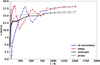 |
Fig. A.1. Illustration of the impact of a binary companion on the velocity field. This is the same as Fig. 10, except it has been replotted with a linear x-axis. |
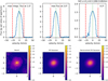 |
Fig. A.2. Determination of the velocity measure and angular emission zone for the SiO v = 0 J=6-5 transition of the medium resolution data of IRC −10529.Top row: The maximum integrated flux is attained for an extraction aperture of 1 |


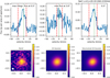 |
Fig. A.3. Determination of the velocity measure and angular emission zone for the NaCl v = 0 J=20-19 transition of the medium resolution data of IRC −10529. The velocity (in km s−1) is with respect to the stellar velocity of −16.3 km s−1 (see the last column in Table 1). The colour scales in the moment0 maps are in units of Jy/beam km s−1 (see Fig. A.2 caption). |
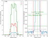 |
Fig. A.4. The J = 2 − 1 line of CO at 230,538.000 MHz observed in T Mic in the compact configuration. The plots show how (in the example of T Mic) the velocity (vmax) was derived from the molecular lines observed in the ATOMIUM survey. Left: The CO spectra extracted with apertures of radius 0.6″ (blue), 1.8″ (red), and 5.4″ (green). Right: The CO profile extracted with an aperture of radius 2.06″ is plotted on an expanded flux density scale with a full scale amplitude of 0.4 Jy/beam to better discern the red and blue wings. The horizontal dashed grey line at 5 mJy beam−1 corresponds to the 1σ peak rms noise (see point #2 in Sect. 5.2); the horizontal dotted grey line at 15 mJy beam−1 corresponds to the 3σ peak rms noise; the green dotted vertical line denotes the line center of CO at the vLSR of +25.5 km/sec; and the red dashed vertical lines indicate the blue wing velocity of −12.7 km s−1, and the red wing velocity of 8.9 km s−1. The value of vmax(CO) with the largest magnitude – i.e., the blue wing velocity of 12.7 km s−1 – is designated as the ‘velocity measure’ of the CO J = 2 − 1 transition in T Mic (see Sect. 5.2). Similarly, the dashed green horizontal line at 76 mJy beam−1 corresponds to the 1σrms noise in the Band 6 spectrum of CO observed in T Mic by Ramstedt et al. (2020, see Table B.1). The dotted green horizontal line at 228 mJy beam−1 corresponds to the 3σrms noise and to the point where the full width of the CO J = 2 − 1 line profile is equal to 12.5 km s−1, whereby Ramstedt et al. determined vmax(CO) = 6.25 km s−1. |
Appendix B: Medium angular resolution spectra of IRC −10529
In this section, we provide the additional spectra extracted from the medium resolution data of IRC −10529 for cubes 02–15. The spectra for cubes 00 and 01 are shown in Fig. 7.
Appendix C: Wind kinematics for 15 ATOMIUM sources
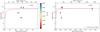 |
Fig. C.3. Wind kinematics for U Del. See Fig. 11 caption. Not enough data are available for a reliable determination of the β parameter. |
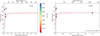 |
Fig. C.4. Wind kinematics for V PsA. See Fig. 11 caption. Not enough data are available for a reliable determination of the β parameter. |
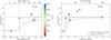 |
Fig. C.5. Wind kinematics for SV Aqr. See Fig. 11 caption. Not enough data are available for a reliable determination of the β parameter. |
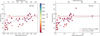 |
Fig. C.9. Wind kinematics for AH Sco. See Fig. 11 caption. Wind velocity profile constructed only on the basis of the medium and high spatial resolution data, since the low spatial resolution data still need to be acquired. |
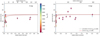 |
Fig. C.10. Wind kinematics for R Aql. See Fig. 11 caption. |
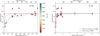 |
Fig. C.11. Wind kinematics for GY Aql. See Fig. 11 caption. |
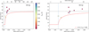 |
Fig. C.12. Wind kinematics for KW Sgr. See Fig. 11 caption. Wind velocity profile constructed only on the basis of the medium and high spatial resolution data, since the low spatial resolution data still need to be acquired. Not enough data are available for a reliable determination of the β parameter. Since the 12CO v = 0 J = 2 − 1 remains undetected in the medium-resolution data, the CO extent is deduced from the high-resolution data. |
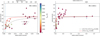 |
Fig. C.13. Wind kinematics for IRC +10011. See Fig. 11 caption. |
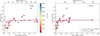 |
Fig. C.14. Wind kinematics for VX Sgr. See Fig. 11 caption. |
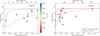 |
Fig. C.15. Wind kinematics for RW Sco. See Fig. 11 caption. |
Appendix D: Determining the terminal wind velocity and the impact of pulsation-induced shocks on the velocity measure
In the main paper, we argue that the 12CO v = 0 J = 2 − 1 line in the low resolution ATOMIUM data can be used to determine the terminal wind velocity, and its integrity as a diagnostic is not perturbed by pulsation-induced shocks that occur in the innermost few stellar radii. We base our arguments on theoretical simulations of a smooth spherically symmetric wind in which the parameters resemble R Aql (see Table 1). The level populations and corresponding intensities of CO in the simulations were computed on the assumption of a CO abundance of [CO/H2] = 2×10⁻⁴ with the (3D) non-LTE radiative transfer code MAGRITTE by De Ceuster et al. (2020a,b) which includes the CMB. The parameters for R Aql resemble the stellar parameters in Table 1 in the main text. The temperature profile is assumed to be similar to that of Danilovich et al. (2017); Danilovich et al. (2020a): T(r) = T⋆(R⋆/r)0.65; and the collisional rates and Einstein A coefficients were taken from the LAMDA database (van der Tak et al. 2020; Yang et al. 2010; Schöier et al. 2005).
In the first set of models, the wind velocity profile follows the analytic expression of Eq. (4) with parameters v0 = 1 km s−1, v∞ = 12.8 km s−1, and β = 1, or 5. Depicted in Fig. D.1 are the 12CO v = 0 J = 2 − 1 velocity measures as a function of the aperture size. It is evident that the CO velocities grow when the aperture size increases from small to large scales. The velocity measure can be larger than the input terminal wind velocity of 12.8 km s−1, owing to the effect of thermal broadening ( ) and turbulent broadening (vturb = 1.5 km s−1) that is accounted for in the full width at half maximum of the Gaussian broadened profile (i.e., FWHM =
  , where
  ). An increase in sensitivity of the observations (and hence a lower noise value) yields a more accurate sampling of the weak wings of the line profile where the broadening manifests itself – particularly in the case of optically thick line profiles (De Beck et al. 2012). The blue-wing velocity measure is often smaller than the corresponding red-wing velocity measure, owing to the effect of the blue wing absorption (Morris et al. 1985; Schoenberg 1988).
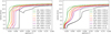 |
Fig. D.1. Change in the 12CO v = 0 J = 2 − 1 velocity measure as a function of the aperture size. The velocity measures are extracted for a range of aperture sizes and noise levels following the same procedure as outlined in Step 2 in Sect. 5.2. The left panel is constructed for a velocity profile with β = 1 and the right panel for β = 5. Velocity measures extracted from the red (blue) wing are indicated with ‘red’ (‘blue’) in the legend in the panels. |
The combined ATOMIUM data is optimal for establishing whether the increase in CO velocities with aperture size is a general trend. To date, the data for the three separate spatial resolutions and the combined dataset are available for six stars: R Hya, π1 Gru, R Aql, IRC −10529, IRC +10011, and VX Sgr, but only π1 Gru has been analysed in detail (Homan et al. 2020). Shown in Fig. D.2 is the change in velocities of the 12CO v = 0 J = 2 − 1 and 28SiO v = 0 J=5-4 lines with aperture size when they are extracted from the combined datasets for the 6 sources by following Step 1 and Step 2 in Sect. 5.2. In Fig. D.2 we also compare the velocity profiles with the velocity measure extracted from the low-resolution ATOMIUM data for the 12CO v = 0 J = 2 − 1 line [see  (CO) in column (3) of Table 3]. For most sources – except for the blue-shifted velocity in IRC +10011, and the red-shifted velocity in R Hya – the CO velocity grows with increasing aperture size and reaches a plateau beyond ∼100 stellar radii. The velocity measure [
 (CO)] derived from the 12CO v = 0 J = 2 − 1 data at low angular resolution is a good tracer for the plateau and the terminal wind velocity, provided the thermal broadening, the turbulent broadening, and the spectral resolution of ∼1.3 km s−1 are accounted for.
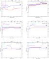 |
Fig. D.2. 12CO v = 0 J = 2 − 1 and 28SiO v = 0 J=5-4 wind velocities of R Hya, π1 Gru, R Aql, IRC −10529, IRC +10011, and VX Sgr. Plots of the blue and red wing velocity of the 12CO v = 0 J = 2 − 1 line (in blue and red, respectively) and the 28SiO v = 0 J=5-4 line (in cyan and pink, respectively) derived from the ATOMIUM combined dataset for a range of extraction apertures for R Hya, π1 Gru, R Aql, IRC −10529, IRC +10011, and VX Sgr, by following Step 1 and Step 2 in Sect. 5.2. The black star (⋆) denotes the 12CO v = 0 J = 2 − 1 velocity extracted from the ATOMIUM low-resolution data, and the error bar denotes the approximate spectral resolution of 1.3 km s−1. |
Understanding how pulsation-induced shocks might impact the velocity measure has a strong bearing on the interpretation of the observationally derived wind kinematics discussed in Sect. 5.4. Analogous to Fig. D.1, we used the non-LTE radiative transfer code MAGRITTE (De Ceuster et al. 2020a,b), but this time rather than using the standard beta-law wind profiles from Eq. (4), the wind velocity profile has been modified to mimic the effect of pulsation-induced shocks within a 1D wind geometry. We used the results of Bladh et al. (2019, see their Fig. 1), which we extrapolated to larger distances from the star by using a fit that follows a beta-velocity profile (see left panel in Fig. D.3). The output image is then run through the ALMA simulator tool for setups resembling the compact, medium, and extended configurations. The simulated output data are then treated in the same way as the ATOMIUM data for the extraction of the velocity measure as a function of the aperture size by following Step 1 and Step 2 in Sect. 5.2 (see the panels labelled ‘normal shock’ model in Fig. D.4). Two main conclusions can be drawn from comparing the ‘no shock’ (upper row) and ‘normal shock’ (middle row) panel of 12CO v = 0 J = 2 − 1: (1) for the case in which the velocity of the shock amplitude is lower than the terminal wind velocity, it is apparent that the velocity measure extracted from the compact CO v = 0 J = 2 − 1 data is the same for the ‘no shock’ and ‘normal shock’ model, confirming that the compact CO v = 0 J = 2 − 1 data is a good measure of the terminal wind velocity (if the effect of thermal and turbulent broadening, and the spectral resolution of the ATOMIUM data are accounted for); and (2) the velocity measures derived from the 12CO extended configuration data are slightly higher if shocks are accounted for, with the shocks manifesting themselves in the faint more extended wings.
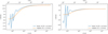 |
Fig. D.3. Wind velocity profile mimicking pulsation-induced shocks just above the stellar atmosphere. The orange curve shows a beta velocity wind profile for β = 5 and v0 = 1 km s−1. The blue curve in the left panel is constructed by: (i) using the shock velocity modelled by Bladh et al. (2019, see their Fig. 1) up to ∼10 R⋆ followed by; (ii) a beta velocity profile that is fitted through the velocity points beyond ∼8 R⋆, with β = 5 and the fit parameter v0 which produces a smooth transition from the pulsation-dominated region towards the freely expanding wind region. In the right panel, the blue curve is constructed in a similar way as in the left panel, but this time the shock velocities modelled by Bladh et al. (2019) are multiplied by a factor of 3. |
We also computed the SiO v = 0 J=5-4 intensities by following the same procedure as for CO (see right hand panels in Fig. D.4). To account for the depletion of SiO by dust condensation and its potential dissociation, the relative abundance distribution of SiO was assumed to follow a Gaussian of the form (Decin et al. 2010b; Danilovich et al. 2014)
![Mathematical equation: $$ \begin{aligned}{}[{\mathrm{SiO/H_2}}] = 3 \times 10^{-5} \exp \left(-(r/r_e)^2\right), \end{aligned} $$](/articles/aa/full_html/2022/04/aa40431-21/aa40431-21-eq65.gif) (D.1)
(D.1)
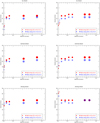 |
Fig. D.4. Simulated wind velocity measures for 12CO v = 0 J=2=1 (left) and 12SiO v = 0 J=5-4 (right). The upper row depicts the model without shocks, the middle (bottom) row the shocked wind model for the velocity profile shown in the left (right) panel of Fig. D.3. The calculated intensities of 12CO and 12SiO account for the different array configurations and extraction apertures in ATOMIUM (see Sect. 3 for details). The velocity measures for the extended (small dots), medium (medium-sized dots), and compact (large dots) configurations were extracted by following Step 1 and Step 2 in Sect. 5.2. The blue dots representing the blue wing velocities are slightly transparent to allow for visualising the red wing velocities in cases where the red and blue dots coincide. |
where the e-folding radius re (2.3 × 1016 cm) was determined by following González Delgado et al. (2003). In spite of its lower abundance, the detectable extent of the SiO v = 0 J=5-4 line observed in the extended configuration is a factor ∼2 larger than for CO v = 0 J = 2 − 1 (0 09 versus 0
 04), establishing the radiative nature of SiO (see Sect. 5.4.2). Analogous to CO, the effect of pulsation-induced shocks in the first few stellar radii — where velocities of around 7 – 12 km s−1 are greater than the local sound speed – are observed in the smallest extraction apertures of the extended configuration data. As Fig. D.4 demonstrates, observations with spatial resolution better than 0
 150 are a prerequisite for characterizing this complex region in more detail.
The question still remaining is whether and how physical phenomena yielding a velocity amplitude greater than the terminal wind velocity manifest themselves in the velocity measure. We therefore take an extreme example and multiply the shock amplitudes from Bladh et al. (2019) by a factor 3 (see right panel of Fig. D.3), where the outcome of the velocity measures are shown in the bottom panels of Fig. D.4 and are referred to as the ‘strong shock’ model. Here as well, several interesting conclusions can be drawn: (1) the compact configuration data of the 12CO v = 0 J = 2 − 1 line are not affected by the presence of shocks in the inner wind, and hence these data are a reliable tracer of the terminal wind velocity given the line broadening and spectral resolution of the data; (2) the extended configuration data of both the 12CO v = 0 J = 2 − 1 and 28SiO v = 0 J=5-4 line bear a signature of the extreme shock velocities in the first few stellar radii of the circumstellar envelope, especially in the case of SiO ; and (3) the extreme shock velocities are not traced in both the medium and compact configuration data. With respect to the latter conclusion, it should be noted that if the rms were three times smaller than the present value, the weak extended wings could be better captured, thereby allowing the (shock) signature to be traced in the low and medium resolution data, although the convolution with the (Gaussian) broadening profile will also be tracked to lower intensity levels and hence yield broader profiles.
Our current physical understanding of pulsation-induced shocks, however, does not validate the use of the ‘strong shock model’, because both models and observations indicate complex, non-monotonic velocity fields with relative macroscopic motions of only some 10 km s−1 (Nowotny et al. 2010). Relying then on the simulations for the ‘normal shock’ model, the question that still needs to be addressed is why the observed SiO velocity measures can be significantly larger than that of CO as shown, for instance, for R Aql in Fig. D.2. Moreover, the same figure shows a trend in SiO velocity measures that is not captured by any of the shock simulations shown in Fig. D.4 in which the medium and compact configuration data roughly show a constant velocity measure. Although detailed modelling of the ATOMIUM wind kinematic profiles is beyond the scope of this paper, the 1D simulations performed here can guide a thought experiment. A binary companion can impact the radial velocity field in a qualitatively similar way as pulsation-induced shocks in the sense that the radial velocity can have a wave-like character (see Fig. 10). The amplitude of the velocity variations will increase for more massive and closer-in companions, and can attain values well above 20 km s−1 where velocity variations of 40 – 60 km s−1 are not an exception (Maes 2020). Guided by the outcome of the ‘strong shock’ models, we stipulate that the particular behaviour of the wind kinematics profile in various ATOMIUM sources can be explained by binary interaction. The high velocities captured in the SiO measurements can be caused by, for instance, the gravitational well of the companion or the formation of an equatorial density enhancement with potentially a Keplerian velocity field similar to the case of L2 Puppis (Kervella et al. 2016).
Appendix E: ATOMIUM image cube properties
Each target’s ‘ALMA name’ is of the form AH_Sco. Each Scheduling Block (SB) is then labelled AH_Sco_a_06_TM1 etc. for the extended configuration, where (a, b, c, d) denote each frequency combination as in Fig. 1. The mid configuration SBs are labelled similarly ending in TM2. The compact configuration data is labelled AH_Sco_e_06_TM1 etc. where (e, f) denote each frequency combination as in Fig. 1. However, for a few targets in compact, inconsistent capitalisation was used for the target names and thus for the SBs. We made these consistent during data processing; the actual observing SB names are also given in Table E.1. The science spw in each SB tuning are numbered 25, 27, 29, 31 in ascending frequency. In the concatenated visibility data files, the spw become re-numbered in the order of observing time (thus, differing from target to target). For the final cubes that can be retrieved from the ATOMIUM website, we re-numbered these in frequency order 00, 01, ⋯, 15. Tables E.2 and E.3 list the properties of each continuum and of each cube image, respectfully.
Observational properties of the ATOMIUM project.
Continuum image properties.
Image cube properties.
All Tables
All Figures
|
Fig. 1. Frequency coverage of the ATOMIUM project in each array configuration (see Sect. 3.1 and Table 2). Each black bar represents the frequency coverage of a spectral window (spw), labelled with the same index number as in our final released data products. The solid lines and letters a–d represent the frequency tunings for the medium and extended configurations; the dotted lines and grey letters e, f represent the frequency tunings for the compact configuration. The exact spectral coverage for each target depends on the adjustment to the assumed vLSR on the dates of observation (see Table 1). Each frequency tuning covered 4 spws grouped as follows: [00,01,04,05], [02,03,06,07], [08,09,12,13], and [10,11,14,15]. The first (second) pair of spw in each frequency tuning corresponds to the lower (upper) sideband in which the channel numbering is in descending (ascending) frequency order. The coloured lines represent the atmospheric percentage transmission labelled by the precipitable water vapour (PWV), in mm. |
| In the text | |
|
Fig. 2. Continuum-maps of IRC −10529. Low (left panel), medium (middle panel), and high (right panel) spatial resolution continuum map. Contours (in orange) are indicated in steps of (3, 6, 10, 100) |
| In the text | |
|
Fig. 3. Low resolution channel map of 12CO v = 0 J = 2 − 1 in IRC −10529. The peak of the continuum emission is at (0,0). The velocity (in km s−1) is with respect to the stellar velocity of −16.3 km s−1 (see the last column in Table 1), and is indicated in the upper right corner of each panel. The ALMA synthesized beam is shown as a white ellipse in the lower left corner of each panel (see Table E.2). The offsets in right ascension and declination are with respect to the peak of the continuum emission. |
| In the text | |
|
Fig. 4. Medium resolution channel map of SO2v = 0 11(1,11)−10(0,10) in IRC −10529. See Fig. 3 caption. The emission shows a hollow shell structure located at a radius of ∼2 |
| In the text | |
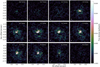 |
Fig. 5. High resolution channel map of SiO v = 0 J = 5 − 4 in IRC −10529. See Fig. 3 caption. |
| In the text | |
|
Fig. 6. SiO moment1-maps of IRC −10529. Low (left panel), medium (middle panel), and high (right panel) spatial resolution moment1-map of SiO v = 0 J = 5 − 4. The black cross indicates the position of the AGB star. The distinct spatial difference between red and blue-shifted velocity components indicates signs of rotation or bipolarity in the inner ∼0 |
| In the text | |
|
Fig. 7. Spectra of IRC−10529. Spectra of IRC −10529 for cubes 00 (left panel) and 01 (right panel) observed in the medium-resolution configuration with ALMA. The spectra were extracted with an aperture whose radius is 1 |
| In the text | |
|
Fig. 8. Illustration of different velocity laws. The full black line at radii beyond 8 R⋆represents the solution of the momentum equation (Eq. (2)) derived for the wind velocity profile of the oxygen-rich AGB star IK Tau (Decin et al. 2010b); for the region between 1–8 R⋆ a beta-velocity law with β = 0.5 is used (Decin et al. 2006). The red dashed line illustrates the β-velocity law (Eq. (4)) for β = 0.5, v0 = 2.7 km s−1, v∞ = 17.68 km s−1, and the vertical black dashed line indicates Rdust at 8.6 R⋆. An almost perfect fit to the velocity as derived from the momentum equation (Eq. (2)) would be obtained for β = 1. The dotted blue line represents the Keplerian velocity law for material bound to a star of mass 1 M⊙. |
| In the text | |
|
Fig. 9. 3D hydrodynamical simulation for a binary system containing a mass-losing AGB star. Slices of density are shown, in units of the density at the sonic point, in the orbital plane (left column) and in the plane containing the orbital axis and the line joining the two bodies (right column). The dimensionless parameters for this simulation are the mass ratio, q = M1/M2 = 1; the ratio of the terminal to orbital speed η = v∞/vorb = 2, the dust condensation radius filling factor f = Rd/RR, 1 = 20% (with RR, 1 the Roche lobe radius of the primary), and the β exponent setting the steepness of the velocity profile here being 5 (El Mellah et al. 2020). For a dust condensation radius set to 3 R⋆, the dimensionless parameters translate into an orbital separation of ∼35 R⋆. Due to binary interaction, a spiral shock is created in the circumstellar envelope. The spiral structure is readily recognised in the density slice in the orbital plane and the width of the successive spiral windings can be deduced from the density arcs in the edge-on view. |
| In the text | |
|
Fig. 10. Illustration of the impact of a binary companion on the velocity field. Given the simulations shown in Fig. 9 (El Mellah et al. 2020), the dotted black line represents the 1D isotropic radial velocity profile (w.r.t. the star). The dotted blue line is the radial velocity profile in the direction of the secondary, and the dotted red line is the radial velocity profile in the direction opposite to the secondary. For comparison, the dashed black curve illustrates the β-velocity law (Eq. (4)) for β = 5 representing the single-star situation. For better comparison with the observed velocity profiles (Sect. 5.2), the same figure but with a linear x-axis is shown in Fig. A.1. See text for more details. |
| In the text | |
|
Fig. 11. Wind kinematics for IRC −10529. The wind velocities for all the molecular transitions observed in the low, medium, and high spatial resolution observations of IRC −10529 derived by the methodology described in Sect. 5.2. The velocities are plotted versus half of the spatial full-width-half-maximum (FWHM) of the molecular emission zone, and represent the dominant line formation region (Decin et al. 2018). The dotted blue vertical line indicates the radius at which the winds begin being accelerated (Rdust in Eq. (4); see Sect. 5.4), and the dotted black horizontal line is the velocity measure of the 12CO v = 0 J = 2 − 1 line. Only emission zones which could be spatially deconvolved are plotted (as dots) – the colour of the symbols are related to the energy of the lower state as indicated by the colour code bar. The grey cross on top of each coloured dot indicates the error bar in the derived velocity and in the FWHM, and is often smaller than the size of the dots. The error bars represent the fitting margin. Not accounted for here are the uncertainties due to the Gaussian approximation which might result in a systematic underestimate of the angular extent (see Sect. 5.2). The bottom axis is in units of arcseconds and the top axis is in units of the stellar radius. Left hand panel: zooms into the 150 stellar radii of the circumstellar envelope, and right hand panel: full extent of the detected wind emission. The 12CO v = 0 J = 2 − 1 transition (indicated in blue) only appears in the right hand panel owing to its large angular extent. The deconvolved data with a velocity less than that of the 12CO J = 2 − 1 transition, were fitted with a β-velocity law (Eq. (4)). Indicated in the legend in the right hand panel is β. The fit is represented by the full grey line which can be compared with a β-velocity law for β = 0.5 indicated by the red dashed line. |
| In the text | |
|
Fig. 12. Wind kinematics for W Aql. See Fig. 11 caption. The vertical blue dashed line at 0 |
| In the text | |
|
Fig. A.1. Illustration of the impact of a binary companion on the velocity field. This is the same as Fig. 10, except it has been replotted with a linear x-axis. |
| In the text | |
|
Fig. A.2. Determination of the velocity measure and angular emission zone for the SiO v = 0 J=6-5 transition of the medium resolution data of IRC −10529.Top row: The maximum integrated flux is attained for an extraction aperture of 1 |
| In the text | |
|
Fig. A.3. Determination of the velocity measure and angular emission zone for the NaCl v = 0 J=20-19 transition of the medium resolution data of IRC −10529. The velocity (in km s−1) is with respect to the stellar velocity of −16.3 km s−1 (see the last column in Table 1). The colour scales in the moment0 maps are in units of Jy/beam km s−1 (see Fig. A.2 caption). |
| In the text | |
|
Fig. A.4. The J = 2 − 1 line of CO at 230,538.000 MHz observed in T Mic in the compact configuration. The plots show how (in the example of T Mic) the velocity (vmax) was derived from the molecular lines observed in the ATOMIUM survey. Left: The CO spectra extracted with apertures of radius 0.6″ (blue), 1.8″ (red), and 5.4″ (green). Right: The CO profile extracted with an aperture of radius 2.06″ is plotted on an expanded flux density scale with a full scale amplitude of 0.4 Jy/beam to better discern the red and blue wings. The horizontal dashed grey line at 5 mJy beam−1 corresponds to the 1σ peak rms noise (see point #2 in Sect. 5.2); the horizontal dotted grey line at 15 mJy beam−1 corresponds to the 3σ peak rms noise; the green dotted vertical line denotes the line center of CO at the vLSR of +25.5 km/sec; and the red dashed vertical lines indicate the blue wing velocity of −12.7 km s−1, and the red wing velocity of 8.9 km s−1. The value of vmax(CO) with the largest magnitude – i.e., the blue wing velocity of 12.7 km s−1 – is designated as the ‘velocity measure’ of the CO J = 2 − 1 transition in T Mic (see Sect. 5.2). Similarly, the dashed green horizontal line at 76 mJy beam−1 corresponds to the 1σrms noise in the Band 6 spectrum of CO observed in T Mic by Ramstedt et al. (2020, see Table B.1). The dotted green horizontal line at 228 mJy beam−1 corresponds to the 3σrms noise and to the point where the full width of the CO J = 2 − 1 line profile is equal to 12.5 km s−1, whereby Ramstedt et al. determined vmax(CO) = 6.25 km s−1. |
| In the text | |
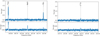 |
Fig. B.1. ALMA spectra of IRC −10529. Caption; see Fig. 7. Data are displayed for cubes 02 to 03. |
| In the text | |
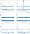 |
Fig. B.2. ALMA spectra of IRC −10529. Caption; see Fig. 7. Data are displayed for cubes 04 to 09. |
| In the text | |
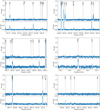 |
Fig. B.3. ALMA spectra of IRC −10529. Caption; see Fig. 7. Data are displayed for cubes 10 to 15. |
| In the text | |
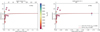 |
Fig. C.1. Wind kinematics for S Pav. See Fig. 11 caption. |
| In the text | |
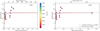 |
Fig. C.2. Wind kinematics for T Mic. See Fig. 11 caption. |
| In the text | |
|
Fig. C.3. Wind kinematics for U Del. See Fig. 11 caption. Not enough data are available for a reliable determination of the β parameter. |
| In the text | |
|
Fig. C.4. Wind kinematics for V PsA. See Fig. 11 caption. Not enough data are available for a reliable determination of the β parameter. |
| In the text | |
|
Fig. C.5. Wind kinematics for SV Aqr. See Fig. 11 caption. Not enough data are available for a reliable determination of the β parameter. |
| In the text | |
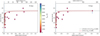 |
Fig. C.6. Wind kinematics for R Hya. See Fig. 11 caption. |
| In the text | |
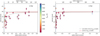 |
Fig. C.7. Wind kinematics for U Her. See Fig. 11 caption. |
| In the text | |
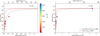 |
Fig. C.8. Wind kinematics for π1 Gru. See Fig. 11 caption. |
| In the text | |
|
Fig. C.9. Wind kinematics for AH Sco. See Fig. 11 caption. Wind velocity profile constructed only on the basis of the medium and high spatial resolution data, since the low spatial resolution data still need to be acquired. |
| In the text | |
|
Fig. C.10. Wind kinematics for R Aql. See Fig. 11 caption. |
| In the text | |
|
Fig. C.11. Wind kinematics for GY Aql. See Fig. 11 caption. |
| In the text | |
|
Fig. C.12. Wind kinematics for KW Sgr. See Fig. 11 caption. Wind velocity profile constructed only on the basis of the medium and high spatial resolution data, since the low spatial resolution data still need to be acquired. Not enough data are available for a reliable determination of the β parameter. Since the 12CO v = 0 J = 2 − 1 remains undetected in the medium-resolution data, the CO extent is deduced from the high-resolution data. |
| In the text | |
|
Fig. C.13. Wind kinematics for IRC +10011. See Fig. 11 caption. |
| In the text | |
|
Fig. C.14. Wind kinematics for VX Sgr. See Fig. 11 caption. |
| In the text | |
|
Fig. C.15. Wind kinematics for RW Sco. See Fig. 11 caption. |
| In the text | |
|
Fig. D.1. Change in the 12CO v = 0 J = 2 − 1 velocity measure as a function of the aperture size. The velocity measures are extracted for a range of aperture sizes and noise levels following the same procedure as outlined in Step 2 in Sect. 5.2. The left panel is constructed for a velocity profile with β = 1 and the right panel for β = 5. Velocity measures extracted from the red (blue) wing are indicated with ‘red’ (‘blue’) in the legend in the panels. |
| In the text | |
|
Fig. D.2. 12CO v = 0 J = 2 − 1 and 28SiO v = 0 J=5-4 wind velocities of R Hya, π1 Gru, R Aql, IRC −10529, IRC +10011, and VX Sgr. Plots of the blue and red wing velocity of the 12CO v = 0 J = 2 − 1 line (in blue and red, respectively) and the 28SiO v = 0 J=5-4 line (in cyan and pink, respectively) derived from the ATOMIUM combined dataset for a range of extraction apertures for R Hya, π1 Gru, R Aql, IRC −10529, IRC +10011, and VX Sgr, by following Step 1 and Step 2 in Sect. 5.2. The black star (⋆) denotes the 12CO v = 0 J = 2 − 1 velocity extracted from the ATOMIUM low-resolution data, and the error bar denotes the approximate spectral resolution of 1.3 km s−1. |
| In the text | |
|
Fig. D.3. Wind velocity profile mimicking pulsation-induced shocks just above the stellar atmosphere. The orange curve shows a beta velocity wind profile for β = 5 and v0 = 1 km s−1. The blue curve in the left panel is constructed by: (i) using the shock velocity modelled by Bladh et al. (2019, see their Fig. 1) up to ∼10 R⋆ followed by; (ii) a beta velocity profile that is fitted through the velocity points beyond ∼8 R⋆, with β = 5 and the fit parameter v0 which produces a smooth transition from the pulsation-dominated region towards the freely expanding wind region. In the right panel, the blue curve is constructed in a similar way as in the left panel, but this time the shock velocities modelled by Bladh et al. (2019) are multiplied by a factor of 3. |
| In the text | |
|
Fig. D.4. Simulated wind velocity measures for 12CO v = 0 J=2=1 (left) and 12SiO v = 0 J=5-4 (right). The upper row depicts the model without shocks, the middle (bottom) row the shocked wind model for the velocity profile shown in the left (right) panel of Fig. D.3. The calculated intensities of 12CO and 12SiO account for the different array configurations and extraction apertures in ATOMIUM (see Sect. 3 for details). The velocity measures for the extended (small dots), medium (medium-sized dots), and compact (large dots) configurations were extracted by following Step 1 and Step 2 in Sect. 5.2. The blue dots representing the blue wing velocities are slightly transparent to allow for visualising the red wing velocities in cases where the red and blue dots coincide. |
| In the text | |
Current usage metrics show cumulative count of Article Views (full-text article views including HTML views, PDF and ePub downloads, according to the available data) and Abstracts Views on Vision4Press platform.
Data correspond to usage on the plateform after 2015. The current usage metrics is available 48-96 hours after online publication and is updated daily on week days.
Initial download of the metrics may take a while.