| Issue |
A&A
Volume 674, June 2023
|
|
|---|---|---|
| Article Number | A125 | |
| Number of page(s) | 74 | |
| Section | Interstellar and circumstellar matter | |
| DOI | https://doi.org/10.1051/0004-6361/202245193 | |
| Published online | 15 June 2023 | |
ATOMIUM: Probing the inner wind of evolved O-rich stars with new, highly excited H2O and OH lines
1
Laboratoire d'Astrophysique de Bordeaux, Univ. Bordeaux, CNRS, B18N, allée Geoffroy Saint-Hilaire,
33615
Pessac, France
e-mail: This email address is being protected from spambots. You need JavaScript enabled to view it.
2
Institut de Radioastronomie Millimétrique,
300 rue de la Piscine,
38406
Saint-Martin-d'Hères, France
3
The University of Manchester, Jodrell Bank Centre for Astrophysics,
Manchester
M13 9PL, UK
4
Universität zu Köln, I. Physikalisches Institut,
50937
Köln, Germany
5
Institute of Astronomy, KU Leuven,
Celestijnenlaan 200D,
3001
Leuven, Belgium
6
National Astronomy Research Institute of Thailand,
260 Moo 4,
Chiangmai
50180, Thailand
7
Chalmers University of Technology, Onsala Space Observatory,
43992
Onsala, Sweden
8
Harvard-Smithsonian Center for Astrophysics,
Cambride MA
02138, USA
9
Department of Physics and Astronomy, Uppsala University,
Box 516,
75120
Uppsala, Sweden
10
Max-Planck-Institut für Radioastronomie,
53121
Bonn, Germany
11
Department of Chemistry and Molecular Biology, University of Gothenburg,
40530
Göteborg, Sweden
12
Astrophysics Research Centre, School of Mathematics and Physics, Queen’s University Belfast,
Univ. Road,
Belfast
BT7 1NN, UK
13
LESIA, Observatoire de Paris, Univ. Paris 5, CNRS,
5 place Jules Janssen,
92195
Meudon, France
14
University of Leeds, School of Chemistry,
Leeds
LS2 9JT, UK
15
School of Physics and Astronomy, Monash University,
Wellington Road, Clayton
3800,
Victoria, Australia
Received:
12
October
2022
Accepted:
2
April
2023
Abstract
Context. Water (H2O) and the hydroxyl radical (OH) are major constituents of the envelope of O-rich late-type stars. Transitions involving energy levels that are rotationally or vibrationally highly excited (energies ≳4000 K) have been observed in both H2O and OH. These and more recently discovered transitions can now be observed at a high sensitivity and angular resolution in the inner wind close to the stellar photosphere with the Atacama Large Millimeter/submillimeter Array (ALMA).
Aims. Our goals are: (1) to identify and map the emission and absorption of H2O in several vibrational states, and of OH in Λ-doubling transitions with similar excitation energies; and (2) to determine the physical conditions and kinematics in gas layers close to the extended atmosphere in a sample of asymptotic giant branch stars (AGBs) and red supergiants (RSGs).
Methods. Spectra and maps of H2O and OH lines observed in a 27 GHz aggregated bandwidth and with an angular resolution of ~0."02−1."0 were obtained at two epochs with the main ALMA array. Additional observations with the Atacama Compact Array (ACA) were used to check for time variability of water transitions. Radiative transfer models of H2O were revisited to characterize masing conditions. Up-to-date chemical models were used for comparison with the observed OH/H2O abundance ratio.
Results. Ten rotational transitions of H2O with excitation energies ~4000–9000 K were observed in vibrational states up to (υ1,υ2,υ3) = (0,1,1). All but one are new detections in space, and from these we have derived accurate rest frequencies. Hyperfine split Λ-doubling transitions in υ = 0, J = 27/2 and 29/2 levels of the 2Π3/2 state, as well as J = 33/2 and 35/2 of the 2Π1/2 state of OH with excitation energies of ~4780–8900 K were also observed. Four of these transitions are new detections in space. Combining our measurements with earlier observations of OH, the υ = 0 and υ = 1 Λ-doubling frequencies have been improved. Our H2O maps show compact emission toward the central star and extensions up to twelve stellar radii or more. The 268.149 GHz emission line of water in the υ2 = 2 state is time variable, tends to be masing with dominant radiative pumping, and is widely excited in AGBs and RSGs. The widespread but weaker 262.898 GHz water line in the υ2 = 1 state also shows signs of maser emission. The OH emission is weak and quasithermally excited. Emission and absorption features of H2O and OH reveal an infall of matter and complex kinematics influenced by binarity. From the OH and H2O column densities derived with nonmasing transitions in a few sources, we obtain OH/H2O abundance ratios of ~(0.7–2.8) × 10−2.
Key words: stars: AGB and post-AGB / supergiants / circumstellar matter / line: identification / instrumentation: interferometers / masers
© The Authors 2023
 Open Access article, published by EDP Sciences, under the terms of the Creative Commons Attribution License (https://creativecommons.org/licenses/by/4.0), which permits unrestricted use, distribution, and reproduction in any medium, provided the original work is properly cited.
This article is published in open access under the Subscribe to Open model. This email address is being protected from spambots. You need JavaScript enabled to view it. to support open access publication.
1 Introduction
Water and the hydroxyl radical are formed from two of the three most abundant elements in the Universe. Many H2O and OH lines have now been observed in the radio, infrared, or visible domains in a broad range of astronomical objects ranging from the planetary and cometary atmospheres of our Solar System to the envelopes of evolved stars or the star-forming regions of our Galaxy. We note that H2O and OH are also present in the disks or nuclei of nearby and distant galaxies. The first radio identification of OH was reported at an 18-cm wavelength by Weinreb et al. (1963) in absorption toward the supernova remnant Cassiopeia A, and the 22.235 GHz (1.35 cm) radio signature of H2O was first reported by Cheung et al. (1969) in star-forming regions and by Knowles et al. (1969) in the red supergiant (RSG) VY CMa. These two centimeter-wave transitions often give rise to a remarkably bright cosmic maser emission which has been observed throughout the Universe in many different regions, including those near the massive black holes of active galactic nuclei (e.g., 22.235 GHz image of NGC 3079, Kondratko et al. 2005). In addition to the strong H2O and OH 1.35- and 18-cm wave radiation, various rotational transitions of water in the ground and vibrationally excited states have been identified in several Galactic late-type stars from ground-based observatories (e.g., Menten & Melnick 1989; Menten et al. 1990a; Melnick et al. 1993; Menten & Young 1995; Gonzalez-Alfonso et al. 1998) or from space (e.g., Justtanont et al. 2012). Recently, Khouri et al. (2019) used their own and archival Atacama Large Millimeter/submillimeter Array (ALMA) data to identify highly excited OH transitions in a few O-rich evolved stars. In star-forming regions of the Galaxy, various rotationally excited transitions of H2O and a few low-lying energy transitions of OH have also been reported (e.g., Menten et al. 1990a,b; Baudry et al. 1997; Harvey-Smith & Cohen 2005; Hirota et al. 2012, 2014). Due to the absorption of water vapor from the Earth’s atmosphere, astronomical observations of H2O are difficult. Nevertheless, high-lying energy transitions of water are accessible from Earth’s dry sites or from airborne telescopes (see e.g., references above, review by Humphreys (2007) or Tables 1 and 2 in Gray et al. (2016) predicting that several H2O lines are observable by (sub)millimeter telescopes). Many lines of water vapor remain, however, inaccessible inside the terrestrial atmosphere (e.g., the 11,0−10,1 transition at 556.936 GHz) and can only be observed from space observatories, such as the Infrared Space Observatory (ISO; Neufeld et al. 1996; Barlow et al. 1996), the Submillimeter Wave Astronomy Satellite (SWAS; Harwit & Bergin 2002), the Odin satellite (Justtanont et al. 2005), and the Herschel Space Observatory (Decin et al. 2010). The role played by these space missions in our understanding of the interstellar water chemistry is described in van Dishoeck et al. (2013), for example.
In parallel with the observational work, chemical models have been developed to explain the ubiquitous presence of H2O and OH. In the general interstellar medium, the review work of van Dishoeck et al. (2021) demonstrates that these two molecular species are essential to explain the O budget of the molecular products observed in star-forming regions. Furthermore, H2O and OH are also known to play a central role in the production of many other species observed in the envelopes of evolved O-rich stars where they are the principal oxidizing agents (e.g., Cherchneff 2006), and they are essential to the dust nucleation processes leading, ultimately, to the formation of circumstellar dust grains (e.g., Gobrecht et al. 2022).
For the purposes of this study, we primarily used our discovery of highly excited H2O and OH radio lines (above ~4000 K) to probe the photospheric environment and the dust formation zone of O-rich late-type stars. As the nuclear burning reactions diminish in the stellar core, the O-rich stars, depending on their initial masses, evolve along the asymptotic giant branch (AGB) or the red supergiant (RSG) branch. The late evolutionary stages of these stars stem from complex mechanisms involving convection, stellar pulsation-driven wind, and shocks that can levitate stellar material above the photosphere. Many millimeter and submillimeter radio observations have shown that shocks and stellar winds offer the favorable conditions that stimulate an active gas chemistry (e.g., Justtanont et al. 2012; Alcolea et al. 2013; Velilla-Prieto et al. 2017; Gottlieb et al. 2022), including OH and H2O that are formed near the photosphere. The Herschel/HIFI observations also provided the abundance of cool water in M-type AGB stars (Khouri et al. 2014; Maercker et al. 2016). Clearly, the nonequilibrium conditions observed beyond the photosphere facilitate the formation of dust-forming clusters in O-rich stars (Gobrecht et al. 2016, 2022; Boulangier et al. 2019) which later form the circumstellar dust grains.
The size of the dust formation zone around evolved stars was first estimated by infrared interferometry (e.g., Danchi et al. 1994). It has later been refined with radio interferometers in the continuum and in the SiO lines which give the size of the molecular shell centered on the photosphere (e.g., Cotton et al. 2004). The dust formation zone encompasses the warm molecular envelope invoked by Tsuji et al. (1997) to explain the observations made with the ISO grating spectrometer and the molecular layers observed in near-infrared molecular bands and modeled by Perrin et al. (2004). This zone is within the radio photosphere first described in Reid & Menten (1997). Beyond the dust formation region, the radiation pressure on the dust particles accelerates the gas flow to outer circumstellar layers (e.g., Höfner & Olofsson 2018), extending to hundreds of stellar radii (R*).
The present work focuses on the identification and interpretation of new H2O and OH radio lines excited at energy levels in the range ~3900–9000 K (~2700–6300 cm−1). These lines, observed in O-rich late-type stars, allowed us to probe the hot and dense gas above the photosphere and in the dust formation zone of the inner circumstellar wind. We adopted the inner wind terminology to include regions covering from the stellar surface to a few R* and up to ~30 R* within which the dust was formed, the wind was launched, and where active gas and dust interactions were observed. Our data were acquired during the ALMA Cycle 6 Large Program 2018.1.00659.L (Decin et al. 2020; Gottlieb et al. 2022). The main objectives of this program, named ATOMIUM, include the study of the molecular paths leading to the formation of the dust precursors as well as the study of the inner (≲30 R*) and intermediate (~30 to hundreds of R*) stellar wind morphology.
In Sect. 2 we present the observed sources (Sect. 2.1), main ALMA array observations (Sect. 2.2), and supplementary ALMA Compact Array (ACA) observations of H2O and other molecules (Sect. 2.3). Table 1 gives the ATOMIUM source sample and the radio detection (or not) of highly excited H2O and OH transitions in the stellar atmosphere of the ATOMIUM stars. Identification of H2O and OH transitions as well as some spectroscopy background for these two species are given in Sect. 3. Several stars exhibit very rich H2O and OH spectra (Tables 5 and 8) and a few of them display all or most of the H2O and OH lines reported in this work (e.g., R Hya). The source spectra and maps, and a first analysis of our data are presented in Sects. 4 and 5 for H2O, and in Sects. 8 and 9 for OH. The widespread 268.149 and 262.898 GHz H2O emissions and H2O maser modeling are discussed in Sects. 6 and 7, respectively. Furthermore, H2O and OH chemical considerations and the OH/H2O abundance ratio in the inner wind of AGBs are discussed in Sect. 10. Concluding remarks are given in Sect. 11 specifying the (sub)sections where the main results are acquired. The Appendices provide the OH Λ-doubling transitions and further H2O and OH spectra and maps.
2 Source sample and observations
2.1 Source sample
The ATOMIUM source sample includes seventeen O-rich evolved AGB or RSG stars covering a relatively broad range of properties in terms of variability type and mass-loss rate (Table 1). Sources are ordered by increasing mass-loss rate noting, however, that this rate is uncertain especially for the distant RSGs AH Sco, KW Sgr and VX Sgr. The source coordinates are obtained from the emission peak of 2D-Gaussian fits to the stellar continuum observed around 241.8 GHz with the ALMA extended configuration, see Table E.2 in Gottlieb et al. (2022). The astrometric accuracy is determined by the accuracy of phase referencing and of fitting to the stellar peak; it is in the range 5–10 mas for both factors.
Most of the adopted distances to the Mira and SR variables in Table 1 are extracted from the Gaia DR3 catalog (Gaia Collaboration 2023) which, however, must be used with care if the parallax uncertainties exceed ~20% (Andriantsaralaza et al. 2022). This is not the case here with the exception of GY Aql whose distance has been revised to 410 pc by Andriantsaralaza et al. (2022). For U Her and IRC–10529 we have also adopted the best distance estimates from Andriantsaralaza et al. (2022) and, for the three RSGs and IRC+10011, the distances are taken from VLBI radio measurements or other works as mentioned in Gottlieb et al. (2022). All other source distances in Table 1 are from Gaia DR31 (Gaia Collaboration 2023). The mass-loss rates in Table 1 are taken from Gottlieb et al. (2022); they are updated for GY Aql and IRC–10529 because of their revised distances. The Local Standard of Rest (LSR) velocity used at the time of the ATOMIUM observations of each star is given in the eighth column of Table 1; the ninth column gives the LSR velocity based on a sample of various lines according to Gottlieb et al. (2022). Table 1 also indicates whether at least one highly excited H2O and OH transition is observed in the stellar atmosphere of each source, while the second last and last columns of Tables 2 and 3 give the number of detected sources for each transition.
Main properties of the ATOMIUM stellar sample and H2O, OH detection.
2.2 Main array observations, data reduction, and products
We observed in three array configurations, extended, mid and compact configurations providing angular resolutions of approximately 0.″02–0.″05, 0.″15–0.″3 and 1.″0, respectively, henceforth high, mid and low resolutions. In the present paper, we identify and analyze the H2O and OH lines falling in the observed bandwidth within the total frequency range covering from 213.83 to 269.71 GHz. We observed 16 spectral windows, or cubes, within this range using four tunings (four spectral windows per tuning), giving an actual bandwidth of 26.8 GHz for the extended and mid configurations and 12.9 GHz for the compact configuration. The central frequency and velocity width of the 16 spectral windows are given in Table 2 of Gottlieb et al. (2022). The exact spectral coverage of each window depends on the adjustment to the adopted LSR velocity on the dates of the observations. The frequency tunings for the three array configurations are also specified in Gottlieb et al. (2022). The highest spatial resolution allows us to resolve the inner few, to few tens of stellar radii for sources in our sample. The extended, mid and (where available) compact configuration data were also combined to provide higher sensitivity to the overlapping angular scales, and could be weighted to provide a range of resolutions.
The maximum recoverable angular sizes are ~0.′′4–0.′′6, ~1.′′8–3.′′0 and ~10.′′0 for the high, mid and low resolutions, respectively. Hence, emission which is smooth on larger scales would not be detected. The H2O and OH emission or absorption lines studied here are probably not affected, being much more compact than ~3 arcsec, as they are excited at very high energies and all maps are dominated by compact structures within the inner layers of the stellar envelope. This is verified by comparing the total flux density detected in different configurations.
Our data were acquired between 2018 and 2021. The extended configuration observations were all performed in June and/or July 2019 under good atmospheric conditions with low precipitable water vapor. The exact dates of observations for each line and each source in our sample can be retrieved from Table E.1 in Gottlieb et al. (2022). All observations were calibrated, imaged and continuum-subtracted in CASA2 as described in Sect. 3.2 of Gottlieb et al. (2022). All the data for a specific star and configuration were combined, and aligned on the stellar peak of the first epoch present. When combining configurations, the most accurate measurements, at the highest resolution, were used. After subtracting continuum (mostly stellar) emission, spectral image cubes were made, adjusted to constant frequency in the LSR frame. All imaging is in total intensity (both observed polarizations combined). Standard cubes were made for each tuning with the angular resolution ranges described above, the exact resolutions depending on observing frequency, target elevation and exact array configuration. In most cases, these spectral cubes were used for analysis but, where appropriate, we made additional cubes around specific lines (see, e.g., Sect. 8.2), optimizing the trade-off between sensitivity and synthesized beam size. The continuum and line clean beams are given in Tables E.2 and E.3 of Gottlieb et al. (2022).
Our channel maps are measured in flux density per clean beam which is a surface brightness over an area converted to Gaussian beam units. For simplicity and consistency with many previous publications, we label the map intensity scale as “flux density” in mJy per beam. The typical rms noise outside the line-emission channels is in the range 0.5–1 and ~2 mJy beam−1 for the high and mid resolutions, respectively. The conversion of mJy per beam to brightness temperature in degrees Kelvin is explained in Sect. 5.1. The spectral channel separation of 976.6 kHz in the ALMA correlator gives a velocity resolution of ~1.1 to ~1.3 km s−1 depending on the observing frequency. The flux density scale errors are typically around 10% per array configuration. However, total uncertainties may exceed 10% due to various amplitude and phase noise effects generated during the data reduction, especially when combining observations made at different times. We adopt here a conservative 15% flux density scale uncertainty.
We extracted H2O and OH spectra from our image cubes for various aperture sizes (larger than the synthesised beam and smaller than the maximum recoverable scale), using circular apertures of diameters typically 0.′′08, 0.′′4 and 4.′′0 for the high, mid and low resolution cubes. Comparisons between these (and with the ACA data, Sect. 2.3) showed that in most cases no additional flux was detected in larger apertures except where variability is likely (Sect. 6.1), confirming that we are not resolving out significant emission from these lines. In some cases, the flux density may appear higher at the highest resolution, due to a combination of the lower map noise in these data and possibly less effective “cleaning” of weak emission much smaller than the lower resolutions.
The H2O and OH spectra and maps referred to in this paper are shown in Sects. 4 and 8 and in Appendices D, C, E and F. For both species the extracted spectral lines are non-Gaussian but the brighter channels within a line profile are well identifiable and used in this work (e.g., Table 5) with an uncertainty of a few mJy for the high resolution data. The velocity extent of the identified H2O lines is determined from the blue and red line wing velocities at the 2.5σ level of each detected line as in the ATOMIUM molecular line inventory (Wallström et al., in prep.). The velocity uncertainty is on the order of one channel, ~1.1–1.3 km s−1, for each line wing determination.
The angular extent of the emitting or absorbing H2O and OH regions is determined without beam de-convolution from our channel maps or from the velocity-integrated intensity maps (zeroth moment or mom 0 maps) using the velocity ranges identified in the spectra or channel maps. For simplicity again, the moment 0 maps intensity scale is labeled as integrated intensity in Jy beam−1 km s−1. The angular extent in our clean images is often irregular and cannot be modeled with simple Gaussian or uniform disk profiles. However, typical or maximum H2O and OH extents can be estimated from the maximum and minimum dimensions within the 3σ contour of our channel maps or mom 0 maps. For the most compact H2O emission sources, we have also used in the AIPS (Astronomical Image Processing System) package3 a specific task to fit Gaussian models by least squares to our images (see Sect. 4.5). In OH, despite often irregular emission or absorption contours, we have used a 3σ contour mask in CARTA4 to fit 2D Gaussians to the observed regions (see Sects. 8.2.1 and 8.2.2).
Observable transitions of H216O covered by the ATOMIUM program.
Observable υ = 0 and 1, ΔJ = 0, ΔF = 0 transitions of OH in the ATOMIUM frequency line setting (excluding ΔF = ±1 and very high N, J transitions).
Frequencies of OH Λ-doubling transitions from astronomical observations and comparison with calculated frequencies.
2.3 ACA observations
To follow up on the widespread detection of the 268.149 GHz H2O line in the ATOMIUM sample, we performed standalone observations with the ACA toward a number of ATOMIUM sources. The main goals of the ACA observations are to cover H2O lines at 268.149, 254.040, and 254.053 GHz (see Table 2) at a higher spectral resolution and to measure the H2O line flux densities at an additional epoch. Three high-spectral resolution windows are placed at 268.15 (H2O), 254.04 (H2O), and 255.48 GHz (29SiO υ = 1) at the spectral resolution of 61 kHz (0.07 km s−1) with a bandwidth of 0.25 GHz (at 268.15 GHz) or 0.125 GHz (at 254.04 and 255.48 GHz). In addition, two wide band windows of 2 GHz each are centered at 252.0 and 266.5 GHz at the resolution of 976 kHz (1.1–1.2 km s−1). Observations were carried out under the ALMA project 2019.2.00234.S in September 2021 during the Return to Operations phase of Cycle 7 toward three stars: R Aql, GY Aql, and VY CMa. In this paper, we focus only on the results obtained for R Aql and GY Aql. All ACA data were reduced with the Cycle 8 ALMA pipeline (version 2021.2.0.128) in CASA 6.2.1–7. The products are essentially the same as those delivered to the ALMA Archive after the QA2 process, except that we have manually identified the continuum spectral ranges in our post-delivery pipeline reduction. Furthermore, we have carried out one round of phase-only self-calibration on the continuum of R Aql and GY Aql using the target scan length as the solution interval. The achieved angular resolutions at the 268.149 GHz H2O line are roughly 7.′′4 × 4.′′3 and 6.′′9 × 4.′′4 for R Aql and GY Aql, respectively.
3 H2O and OH spectroscopy, line identification
This section briefly describes the principles leading to the spectroscopic determination of H2O line frequencies (Sect. 3.1) and our line frequency detection criteria (Sect. 3.2). A similar approach is followed for OH in Sects. 3.3 and 3.4. Identification of which H2O and OH lines are observed in which source is given in Tables 4 and 5, respectively.
3.1 The water molecule, spectroscopy background
The rotational and rovibrational energy levels of light hydrides, molecules consisting of one or more H atoms and at most one light non-H atom, are often difficult to describe by a conventional Watson-type Hamiltonian because of the large effects of centrifugal distortion (Pickett et al. 2005). The water molecule, H2O, is a prototype in this regard and an overview of alternative models developed to fit rotational and rovibrational spectra of H2O is presented in Pickett et al. (2005).
H2O is an asymmetric rotor with energy levels described by  where J is the rotational quantum number and Ka and Kc are the projections of the total angular momentum along two of the three axes, a, b and c used to derive the three principal moments of inertia of water. The a-axis is parallel to the H to H direction and orthogonal to the b-axis that crosses the O atom and along which the H2O permanent dipole moment is observed (see right panel in Fig. 1). A precise value of the dipole moment along the b-axis was obtained by Shostak et al. (1991), μ0 = 1.855 D. We point out that vibration and distortion corrections to the dipole moment are required to accurately model intensities and derived quantities (Shostak et al. 1991; Shostak & Muenter 1991; Grechko et al. 2012). H2O has three fundamental vibrational modes, the symmetric stretching mode ν1 and the bending mode ν2 both of a1 symmetry, and the antisymmetric stretching mode ν3 of b2 symmetry. A common shorthand notation to describe any vibrational states is a triplet which indicates the degree of excitation of each fundamental mode in the form (υ1,υ2,υ3). The three fundamental modes of vibration are schematically represented in Fig. 1 and the lowest eight vibrational states of H2O are displayed in Fig. 2 together, as an example, with the (υ1,υ2,υ3)
  upper energy levels of four transitions detected in this work (see Fig. 2 caption and Table 2). The vibrational states (0,2,0), (1,0,0) and (0,0,1) as well as (0,3,0), (1,1,0) and (0,1,1) are quite close in energy (Fig. 2). As a consequence, rotational levels with the same total angular momentum J may interact if they are nearly degenerate and obey certain selection rules (i.e., there may be mutual interaction of nearby, unperturbed levels). Fermi interaction may occur between rotational levels involving the (0,2,0) and (1,0,0), and (0,3,0) and (1,1,0) vibrational states; the quantum numbers of the
  levels need to differ in Ka and Kc by even numbers. The interaction edfects are usually largest if Ka and Kc are identical. Coriolis interaction of c-type may occur between levels involving (1,0,0) and (0,0,1), and (1,1,0) and (0,1,1); the quantum numbers need to differ in Ka by an odd number and in Kc by an even number. The interaction effects are usuatly largest if Ka differs by one. The tnteraction betwera (0,2,0) and (0,0,1), and (0, 3,0) and (0,1,1) is called rotational or Coriolis-type, or, frequently, just Coriolis (C′ in Fig. 2). This is appropriate as the operators describing the interaction are the same as for a proper Coriolis interaction. However, this type of interaction is of higher order and usually has relatively small effects.
The energy difference between two interacting rotational levels is larger than in the noninteracting case and tends to mix levels. One consequence in the case of the Fermi interaction between (0,2,0) and (1,0,0) is that if a transition from one level in (0,2,0) to an interacting level in (0,2,0) is allowed, then a transition from the first level in (0,2,0) to the corresponding interacting level in (1,0,0) is also allowed; the strength of the latter transition depends on the degree of the mixing between the two interacting levels. Such transitions can also occur for other types of vibration-rotation interaction. An additional effect in the rotational spectrum of H2O is that the presence of two equivalent H nuclei leads to spin-statistical weights of three and one for levels of ortho and para H2O, respectively. The ortho and para states for vibrations with a1 symmetry are described by Ka + Kc being odd and even, respectively, while it is the opposite for vibrations with b2 symmetry. The states of a1 and b2 symmetry are labeled in blue and aubergine in Fig. 2, respectively.
The rotational spectrum of H2O in low-lying vibrational states has been investigated extensively. A fairly recent and extensive study of THz and far IR transitions of water in the lowest five vibrational states was published by Yu et al. (2012). Their analysis included numerous transitions in the range 293–2723 GHz (determined with ~1–100 kHz accuracy) and in the 50–600 cm−1 far IR region (with accuracy up to a few tens of MHz). These data, taking into account earlier data, are the current basis for the JPL catalog (Pickett et al. 1998) entries of H2O in its ground vibrational state and in its next four excited vibrational states, (0,1,0), (0,2,0), (1,0,0) and (0,0,1). Shortly thereafter, Yu et al. (2013) determined transition frequencies for the next three vibrational states (the second triad) and redetermined some frequencies in the first five states. Coudert et al. (2014) provided additional transition frequencies of the lowest eight vibrational states in the far IR region; they cover, tn particular, highly rotationally excited states. They also presented a catalog file for the second triad consisting of the (0,3,0), (1,1,0), and (0,1,1) states. Unfortunately, no frequencies have been calculated below 500 GHz.
H2O peak flux density (first entry in mJy) and velocity extent (second entry in km s−1, highlighted with italics) of observed lines for an aperture diameter of 0.′′08 extracted from the extended configuration.
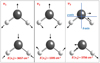 |
Fig. 1 Three fundamental vibrational modes of water vapor. They are denoted v1 and v3 for the symmetric and asyimrietric stretchings, and v2 for the symmetric bending. The arrows simulate me direct and reciprocal vibrational motions of the Ο and the two H atoms (adapted from Schroeder 2002). The Ο to Η bond length is nearly 0.1 nm and the H-O-H average angle is 104°. The a and b axes discussed in Sect. 3.1 intersect at the center of mass of the molecule. The energy of the three fundamental vibrational states v1 ν2, v3 are 3657, 1595 tind 3756 cm−1, respectively; the equivalent stale temperature and warelengths are 5262, 2294 and 5404 K (see also Fig. 2) and 2.73, 6.27 and 2.66 μm. |
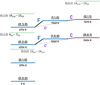 |
Fig. 2 Lowest eight vibrational s)atei of water vapor and their quantum numbers (υ1,υ2,υ3). Stares of a1 symmetry are referred to by horizontal blue lines, states of b2 symmetry by aubergine lines. Vibration-rotation interactions are indicated by lines connecting the interacting states. The labels F, C and C’ symbolize Fermi, Coriolis, and rotational (or Coriolis-type) interactions. The energy of each vibrational band origin is given in Kelvin below each horizontal solid line. The rotational and ro-vibrational transitions in the range of snerau covered by the ATOMIUM project are listed in Table 2. Four examples, corresponding to lines 10, 14, 8 and 4 in Table 2, are shown with their quantum identification, in the form on dotted horizontal green lines; they are ordered by increasing energy. |
3.2 Identification of highly excited water lines
Water vapor has a rich spectrum pure rotational transitions as well as many rovibrational transitions spanning a broad range of wavelengths from the IR to the submm/mm domain. The first excited states of the symmetric and asymmetric stretching modes observed around 2.7 μm (v1 and v3 bands and the first excited state of the bending mode observed at. 6.27 μm (v2 band) are the most important IR transitions of water (Fig. 1). Other vibrational transition bands have tang been identified in the low dispersion astronomical spectra of Mira stars, (e.g., Spinrad & Newburn 1965; Hinkle & Barnes 1979).
The high sensitivity and high spectral resolution achieved with ALMA allow us to search for various ro-vibrational or pure rotational transitions of water in different vibrational states so that a broad range of energies and physical conditions can be probed with an appropriate selection of water transitions. Using the JPL catalog (Pickett et al. 1998)5 and the W2020 data base (Furtenbacher et al. 2020) and, limiting observes to energy levels up to ~6500 cm−1 (9400 K), we have searched for all pure rotational or ro-vibrational dipolar electric transitions of water in our frequency settings, without any a priori spectral line intensity cut-off. We found fourteen transitions of the main isotopic species of water with energy up to ~9000 K; they are listed in Table 2. Ten are safe detections in the present work and were identified in different targets (see last two columns in Table 2 for number of detected sources and spectroscopic references). Six are ortho H216O and four para H216O transitions; one ortho H216O transition is uncertain (line 9 in Table 2; see Appendix C). The first entry in the second and third columns in Table 2 gives the rest frequency and uncertainty from the JPL catalog (c018003 and c018005 files) or from the W2020 data base. The second entry in the second and third columns of Table 2 for lines 1, 4, 5, 6, 7, 8, 10, 12, 13 and 14 gives our own rest frequency measurements and estimated maximum uncertainties (see discussion below). Using the same line selection criterion as above, there are one H217O and four H218O transitions in our frequency setup. None of them are in the ground vibrational state and no signal was observed in the vicinity of the expected frequencies. Moreover, the predicted line intensities are too weak for reliable identification. H2O, and later OH, without superscript in this article, always refer to H216O and 16OH.
We have assigned to H2O the high signal-to-noise ratio (S/N) features identified in our spectra when such features, once corrected for the systemic velocity of the star, coincide within a few MHz with transitions of H2O in the JPL or W2020 data bases. The spectra used for this identification have been extracted from both the high and mid resolution data cubes for different aperture diameters (0.′′08 and 0.′′4 diameters are used in general for high and mid, respectively). The number of sources for which we have a spectral identification as defined above, varies from fifteen (line14 in Table 2) to four (line number 5, in absorption) or just one or perhaps two (line 4, see Appendix C). Line identification did not suffer from spectral confusion problems. In addition, we used the CDMS6 (Müller et al. 2005; Endres et al. 2016) data base to check for possible misidentifications due to the spectral proximity with the molecular species in the ATOMIUM chemical inventory (Wallström et al., in preparation). Lines 4, 6 and 8 in our Table 2 lie close to SO18O at 236.805, 252.185 and 254.067 GHz but only SO2 and 34SO2 are identified in the ATOMIUM inventory. We note the frequency proximity of the H2O line 1 at 222.014 GHz with the υ = 0,  transition of SiC2 at 222.009 GHz, but this species is identified only in the S-type star W Aql which has no water emission.
Despite uncertainties discussed below, we have used the observed emission line peak for a given transition (or the average of a few line channels for flat-emission features) to estimate our own line rest frequency and confirm line identification. The average of our frequency measurements in different stars for a given transition, corrected for the stellar velocity used during the observations, is our observed rest frequency. It is shown in the second column of Table 2 below the JPL or W2020 rest frequency; we add TW (for This Work) as appropriate in the last column of Table 2. (We have not made a frequency estimate for line 5 seen in absorption near 244.330 GHz.) There are a few caveats to our line frequency estimates. Line opacity effects or line profiles skewed by line wing absorption due to gas infall, for example, may eventually bias our measurements. However, the high energy transitions of water studied here are not optically thick in general (Sect. 5.2); for line 14 which tends to be masing in some sources (Sect. 6) specific velocity components could be enhanced, however. We have used as much as possible “well-behaved” line profiles with the hope that averaging independent frequency measurements in different stars minimizes the errors. Our main sources of error most probably come from limited spectral resolution, ~1 MHz, and the stellar velocity uncertainty. The latter uncertainty is small as suggested by comparing the velocities given in the eighth and ninth columns of Table 1. There are eight sources with differences below 0.4 km s−1, or less than 0.36 MHz at 268.149 GHz, and eight other sources with differences ≲0.9−2.0 km s−1 or below 1.8 MHz. Despite all potential errors we find that, for those transitions for which we have a significant number of independent measurements, the variance of our frequency calculations is ≲1 MHz. We adopt 1.5 or 2 MHz as our total frequency uncertainty in Table 2 and note that in spite of various uncertainties, the frequency discrepancy between our calculations and the JPL catalog remains within ~0.2−3 MHz, except for the ~9000 and 8300 K high energy lines 4 and 13 where it is larger. We further note that our rest frequency determinations are in good agreement with those measured in the laboratory; this is well verified for lines 7, 10, 12 and 14 in Table 2. In the case of relatively high uncertainties for the calculated rest frequencies in catalogs our rest frequency determinations could be better, especially for lines 1, 8 and 13.
We stress that, as far as we know, nine out of the ten water transitions detected in this work are new radio detections in space. Line 14 in the υ2 = 2 state at 268.149 GHz is the only transition that was first observed as a strong emission in VY CMa (Tenenbaum et al. 2010) and a weak line in IK Tau (Velilla-Prieto et al. 2017). We find here that this line is excited in twelve AGBs and three RSGs of the ATOMIUM sample. The only two targets without any H2O transition, are the two S-type stars in Table 1 with a water abundance expected to be lower than in the O-rich M-type stars (compare e.g., the 1.5 × 10⁻⁵ water abundance derived by Danilovich et al. 2014 in W Aql with the higher water abundance obtained by Khouri et al. 2014 and Maercker et al. 2016 in M-type stars).
The 268.149 and 262.898 GHz transitions in the (0,2,0) and (0,1,0) states are widespread in evolved stars and will be analyzed in Sect. 6. Line 1 in the (0,3,0) state at 222.014 GHz is the first radio detection of water in such a high vibrational state; it also seems to be widespread in O-rich stars. Finally, we note that the three ro-vibrational transitions without detection in stars, lines 2, 3 and 11, have low spontaneous emission rates (A value) implying weak spectroscopic line strengths. However, the A value for line 6, with eight sources detected, is not much larger than that of line 11 with no detection. We also point out that line 4 with the highest energy levels observed in this work is identified in at most two stars (see footnote in Table 2).
3.3 The OH radical, spectroscopy background
The hydroxyl radical, OH, exhibits a complex spectrum because of its unpaired electron and coupling with the nuclear spin of the hydrogen atom. The electronic ground state of OH is a 2Π state according to the value of one for its electronic orbital angular momentum projection along the OH internuclear axis. Accounting for the spin-orbit coupling, the total electronic angular momentum along the OH axis is described by the quantum number Ω which takes the value 3/2 or 1/2. The OH states are designated 2Π3/2 and 2Π1/2, 2Π3/2 being lower in energy. The spin-orbit splitting of OH is appropriately described by Hund’s case (a) for lower quantum numbers while Hund’s case (b), where the spin is not coupled to the internuclear axis, is more appropriate for higher quantum numbers. In addition, the energy of the weak coupling of the OH rotational angular momentum with the total electronic angular momentum depends on their respective sense of rotation. Hence, each degenerate rotational energy level is split into Λ-doublets with nearby energy levels and different parity. For the higher rotational levels, where case (b) applies, the orbital electronic momentum and the rotational molecular momentum form a resultant vector described by the scalar number N which, combined with the scalar value of the spin vector S = ±1/2, gives J = N + 1/2 and N – 1/2 in the 2Π3/2 and 2Π1/2 states. Hund’s case (b) is appropriate for the ATOMIUM high–J OH observations.
Another weak magnetic coupling between the unpaired electron spin of OH and the hydrogen nuclear spin, described by the total quantum number F = J ± 1/2, is observed at high spectral resolution both in the laboratory and in space. The ΔF = 0 hyperfine transitions within a given Λ-doublet (ΔJ = 0) are called principal (or main) lines because their local thermodynamic equilibrium (LTE) intensities relative to the so-called satellite lines (for which ΔF = ±1) are 5:1 and 9:1 in the 2Π3/2, J = 3/2 ground state; these relative intensities can reach much higher values at higher rotational levels.
There are twelve ΔF = 0 lines of OH in the υ = 0 and 1 vibrational states falling in the ATOMIUM frequency range. They are given in Table 3 and ordered by increasing frequency. We have not included in Table 3 the very weak ΔF = ±1 satellite lines nor the five very weak J = 41/2 – 43/2, ΔF = 0, ±1 transitions in the υ = 0 and 1 vibrational states, although they fall in our frequency setup. (Other weak 17OH and 18OH transitions, which are not observed in our data, are not discussed either.) The rest frequencies, based on rotational spectra of OH and isopotologs (Drouin 2013), and associated errors rounded to ten kHz are taken from the JPL catalog (c017001 file, version 5) and given in the second and third columns of Table 3 together with some relevant quantum numbers, the upper energy level and Einstein-A coefficient. The number of OH sources detected per transition in this work is shown in the last column of Table 3. We note that lines in Tables 3 and 4 can also be identified from their 2Π3/2 or 2Π1/2 electronic ground state. Lines 5 and 8 for example, observed in four and nine different sources, correspond to 2Π1/2, υ = 0, J = 33/2, F′ – F′′ = 17− − 17+ and 2Π3/2, υ = 0, J = 29/2, F′ – F′′ = 15+ − 15− near 236.328 and 252.145 GHz, respectively.
The Λ-doubling frequencies of OH derived from the ALMA observations in this work and in Khouri et al. (2019) are gathered in Table 4. The observed OH frequencies (third column in Table 4) may sometimes differ from the JPL frequencies (second column in Table 3). This discrepancy is commented on in Sect. 3.4 where we also derive new OH Λ-doubling frequencies. The O–C column in Table 4 corresponds to the difference between the frequency derived from the astronomical observations and our new frequency calculation described in Sect. 3.4 and Appendix A.
3.4 Identification of OH lines, improving Λ-doubling frequencies
Identification of the OH lines in the ATOMIUM sample primarily rests on the JPL catalog line frequencies. We have used the observation of a spectral feature at the expected frequency and the observation in our channel maps and spectra of two nearby features with a frequency separation as predicted from an OH Λ-doublet as a secure identification of a Λ-doublet. Four OH Λ-doublets in J = 27/2, 29/2, 33/2 and 35/2 corresponding to seven, and possibly eight, different ΔF = 0 hyperfine transitions have been identified. As for water in Sect. 3.2, we have verified that there is no misidentification with the lines in the ATOMIUM chemical inventory. OH line 10 in J = 35/2 is still uncertain in R Hya (see footnote in Table 3). In Mira (Fig. F.1) as in R Hya, the J = 35/2 line 9 is weakly detected while line 10 is blended with the relatively strong υ = 0, J = 242,22 – 241,23 transition of TiO2 at 265 770.5 MHz. (This TiO2 transition is not present in our R Hya data.) We also note the proximity, but without spectral confusion, of the OH J = 29/2, F′ – F′′ = 15–15 transition (line 8) with the (1,0,0)–(0,2,0)  transition of water at 252.172 GHz (see right-hand panels in Fig. 20). The last column in Table 3 shows that the most frequently detected hyperfine line pairs are observed in the J = 27/2 and 29/2 levels.
For a closer comparison of the observed OH transitions with the JPL catalog frequencies we have derived the hyperfine transition frequencies in the J = 27/2 and 29/2 states after we have extracted the OH spectra for an aperture diameter of 0.′′08 from the high resolution data cubes. The OH line profiles are often slightly asymmetric. However, our stronger OH sources, R Hya, S Pav or R Aql, show well-identified line peaks which we have used with the LSR stellar velocity adopted during the observations to derive the observed rest frequencies. We have also verified that in R Hya, the observed peak frequencies are identical within 0.5 MHz for spectra extracted for a total size region larger than about 0.′′ 1. Optical depth effects of these weak OH lines are not expected to play any significant role in our frequency determinations and, to minimize any possible frequency skew due to gas kinematics, we adopt the average of our frequency measurements obtained from independent observations in different stars as our OH rest frequencies; they are given in Table 4 together with an adopted uncertainty of 1.5 MHz. The lines 6 and 9 in J = 33/2 and 35/2, were observed in one star only, R Hya. In that case the uncertainty is determined from the difference between, the intensity-weighted average of all channels with detected emission, and the direct frequency average of these channels; it is maximized to 2 MHz (Table 4).
Our OH frequency measurements differ by ~2–4 MHz from the JPL frequencies in Table 3 thus exceeding the uncertainties estimated by combining our estimated uncertainties with those quoted in the JPL catalog. (The O–C in Table 4 are nearly always smaller than ~1–2 MHz.) Similarly, Khouri et al. (2019) have noted deviations of up to a few MHz between the calculated Λ-doubling transitions and their radio observations. These discrepancies are, on average, systematic, increasing with J and υ, and cannot be explained by an uncertainty in the observed star’s systemic velocity or by some intrinsic high velocity motions of the gas where the OH lines are excited. In addition, we do not see in our data that the OH emission comes from a single side of the star’s limb. We give at the beginning of Appendix A the various limitations in the laboratory spectroscopic measurements that can explain why our observations, as well as those of Khouri et al. (2019), suffer from deviations up to a few MHz between the calculated and observed Λ-doubling transitions in high-J levels. Details on our improved Λ-doubling calculations for energy levels in the υ = 0 and 1 states from ~1300 to ~10 500 cm−1 are presented in four tables of Appendix A: Tables A.1 and A.2 for the υ = 0, 2Π3/2 and 2Π1/2 states; Tables A.3 and A.4 for the υ = 1,2Π3/2 and 2Π1/2 states7.
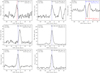 |
Fig. 3 Water line profiles extracted from the extended configuration of the main array for an aperture diameter of 0.′′08 in R Hya. First two rows: six transitions of ortho H2O as defined in Table 2: lines 1, 6, 8 (including line 7 separated by 12.7 MHz, or 15.0 km s−1, from line 8) and lines 13 and 14. Last row: two transitions of para H2O as defined in Table 2: lines 10 and 12. The spectra are converted from the observed frequency to the LSR frame using the H2O catalog Une rest frequencies given in Table 2. In all spectra, the blue vertical line indicates the adopted new LSR systemic velocity as shown in Table1. For line 1 (upper left panel), file red verticad line shows the LSR velocity for the slightly different frequency determined in this work. Spectral resolution varies from ~1.1 km s−1 (268 GHz) to ~1.3 (222 GHz) km s−1. |
4 H2O source properties
4.1 Observation of highly excited transitions of water
As described in Sect 3.2, ten different transitions of water have been identified on the basis of a close coincidence of an observed spectral feature with a transition in the JPL or the W2020 catalog. An overview of the H2O spectral line properties extracted from the high resolution image cubes for a circular aperture of 0.′′08 can be found in Table 5 which brings together the peak line flux density and the uelocity exteni as defined in Sect. 2.2. (Comparing the high resolution spectra with those extracted from the mid resolution data in a 0.′′4 diameter aperture shows that there is no systematic difference in intensity and we consider that the 0.′′08 aperture reveais the spectral behavior of the most compact structucot close to the star and within the muximum recoverable angular size. We also point out that our mid resolution data do not reveal any new H2O transition in any source.
Examples of H2O spectra extracted from the high resolution data cubes in R Hya ate presented Fig. 3; eight out of ten fines of both the ortho and para species are strongly detected in this source. All spectra in all sources have been gathered in Appendix B except those for the taint line 4 emission discussed in Appendix C. H2O tine 5 absorption is shown in Fig. 5 and in Appendix B. As far as we know, the (0,3,0) 83,6–74,3 transition at 222.014 GHz (line 1) is the first ever mm-wave transition observed in the (0,3,0) vibrational state toward several AGBs and RSGs (see Fig. 4 ant all detections in Appendix B). (Throughout this paper we only quote once the vibrational triplet for pure rotational transitions whose quantum numbers are specified without adding  ; for ro-vibrational transitiom we give the two vibrational triplets.)
Because the transitions in Table 5 arise from high-lying levels between ~4000 and 9000 K (note that line 4 at 236.805 GHz has the highest excitation energy), the observed peak line intensities are generally low. Our new detections significantly increase the number of H2O rotationai tranrittons that ate currently ob served with ground-bysed radio telescopes in evolved stars. Therange of excitation energies now extends to much higher values than those observed previously (~470–2400 K). From space, however, water line detections have been reported at high energy levels (e.g.,up to ~7700 K in VY CMa; Alcolea et al. 2013). Apart from line 4 which was observed in only one source (or perhaps two) and line 5 in four sources, all other lines in Table 2 are identified in 4 to 15 ATOMIUM sources (see Table 5 and column ndet in Table 2).
S Pav, R Hya, R Aql and IRC+10011 are the sources in our sample with the richest water vapor spectra (Appendix B). All H2O lines observed in the present work are excited in these four sources, except line 4 which is only observed in R Hya (and perhaps in S Pav). On the other hand, four other sources exhibit only two or three water transitions (RW Sco, V PsA, SV Aqr and GY Aql) and two stare which are generally line-poor U Del and the distant SRc variable KW Sgr, are weakly detected at 268.149 GHz only. We also note that in IRC+10011, despite its large distance, the peak flux: density of each detehed transition, except at 268.149 GHz, tends to be stronger than in other sources.
Although our source sample is small, it does not seem to show any dependence of the Sine detection rate with physical parameters such as the mass-loss rate; in fact, the star with the lowest mass-loss rate, S Pav, exhtbits as many detected transitions as our highest mass-loss rate star, VX Sgr. This is confirmed by the correlation analysis of Wallström et al. (in prep.) between several physical parameter and the number of H2O lines. We note that the line source detection rate observed here tends to increase as the energy of the transition decreases, that is to say lower states (~4000–5600 K) are detected in nearly two times more sources than in higher states (~8000–9000 K). Such a trend is not surprising “a priori” since we expect the highest energy levels to be less easily populated.
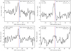 |
Fig. 4 Typical line profiles of the (0,3,0) 83,6 – 74,3 transition of H2O at 222.014 GHz in R Aql, S Pav, IRC+10011 and VX Sgr. The upper left panel in Fig. 3 shows the same transition in R Hya. Spectra are extracted for an aperture diameter of 0.′′ 08 from the extended configuration and converted from the observed frequency to the LSR frame using the H2O catalog; line rest frequency given in Table 2. The red and blue vertical lines indicate the new LSR systemic velocity (see Table 1) corresponding to our frequency determination and to the catalog frequuncy, respectively. The spectral resolution is ~1.3 km s−1. |
4.2 Water line absorption
The absorption of a water line was first observed with the longest baselines of ALMA toward Mira by Wong et al. (2016). Their spatially resolved images of the (0,2,0) 55,0 – 64,3 transition at 232.687 GHz reveal H2O line absorhtion against the background continuum and a line emission region that closely corresponds to that of the highly exctied υ = 2, SiO line. tn our ATOMIUM high-angular resolution data, we also observe both line emission, which is dominant, and weak absorption. At 259.952 GHz (para H2O line 10), absorption is detected at the level ot ~5–15 mJy for the extended configuration and 0.′′08 aperture diameter, together with relatively strong emission toward R Hya (Fig. 3), R Aql, S Pav and U Her. Absorption is also seen in one or two of the nearby frequencies at 254.040 and1 254.053 GHz (lines 7 and 8 in two different vibrational states) in t;he four objects cited above and in IRC–10529, IRC+10011 and T Mic. In R Hya, an absorption feature is observed in Fig. 3 on the redshifted side of the (0,2,0) 143,12–134,9 main emission line profile 254053 GHz and is confirmed by the absorption map of this feature (see end of Sect. 4.4). The para H2O line profile at 244.330 GHz (line 5) shows only absorption, which is in contrast with, for example, the υ = 1, CO(2–1) line profile, expected to be excited in a similar region and that shows both absorption and emission. The spectra of the stronger 244.330 GHz absorption sources are presented in Fig. 5 and compared with those of the υ = 1, J = 2 – 1 high energy transition of CΟ (~4400 K). The water line absorption is spectrally narrow and lies on the red side of the bulk of the CO emission profiles suggesting an infall of the water-bearing matter (see Sect. 4.4).
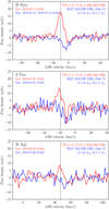 |
Fig. 5 Absorption spectra of para H2O at 244.330 GHz in R Hya, S Pav and RAql (blue profiles) and, emission/absorption spectra of the υ = 1 transition of CO(2−1) at 228.439 GHz in the same sources (red profiles). The spectra are converted from the observed frequency to the LSR systemic velocity using the H2O line 5 (Table 2) and υ = 1, CO(2−1) rest frequencies. All spectra are extracted from the high resolution data cubes for an aperture diameter of 0.′′08. The vertical black dotted lines indicate the adopted new LSR systemic velocities (see Table 1). |
4.3 Channel maps, angular sizes, ring-like structures
Channel maps have been produced for each source in our sample for both the extended and mid array configurations and for all detected transitions listed in Table 2. The angular sizes and structure of the H2O emitting regions observed with the extended configuration are discussed here while the line 5 absorption is presented in Sects. 4.4 and 5.4. To illustrate the discus-lion on the H2O emission, we have selected channel maps for transitions that reflect the variety of excitation conditions, that is maps of the: (i) strong (0,2,0) 65,2–74,3 emission at 268.149 GHz (line 14), but with relatively high excitation energy levels, in R Hya and U Her (Fig. 6), in S Pav and IRC+10011 (Figs. D.1 and D.2), and two RSGs, VX Sgr (Fig. D.3) and AH Sco (Fig. D.4); (ii) two relatively weak transitions, wish close frequencies but with well separated energy levels, (0,0,1) 31,3–22,0 and (0,2,0) 143,12–134,9 (lines 7 and 8) at 254.040 and 254.053 GHz in R Hya (Fig. 7); (iii) relatively low energy transitions (0,0,0) 136,8–143,11 at 259.952GHz (line 10 in R Hya, S Pav, IRC+10011 and VX Sgr, Figs. D.8 and D.9) and (0,1,0) 77,1–86,2 at 262.898 GHz (line 12 in R Hya, U Her, S Pav, IRC+10011, VX Sgr and AH Sco, Figs. D.5–D.7).
The matority of the water emission is closely associated with the underlying continuum source although the emission peak may not exactly coincide with the central star; for more details, readers can refer ro the channel maps in R Hya and U Her at 268.149 GHz (Fig. 6) or at 222.014 GHz in R Hya (Fig. D.10), for example. Weak, diffuse emission is also observed away from the central object and, in a few cases, apparent ring-like structures are preseni in our channel maps (see discussion at the end of this section).
The typical angular sizes of the nonmaser line emission regions are obiained in two different ways from the high resolution channel maps without de-convolving the data trom the clean beam since the surface brightness distribu)ion is irregular and not Gaussian at the high resolution achieved here. In a first approach, sizes are derived from the geometric mean ot the maximum and minimum angular radii of the emission centered on the star and enclosed within the 3σ contour, noting thai the fitting accuracy to the contour is on the order of one third of the beam. In the second approach, the radial distances are obtained from azimuthal averaging of the emission within (he 3σ contour of the moment 0 maps in a manner similar to that used by Danilovich et al. (2021) in W Aql. Compiling our H2O measurements from the two approaches above we find that the angular radii cover the range ~10–50 mas for all stars and all detected lines (reaching ~60 mas for line 14 in AH Sco and IRC+10011). These radii may differ by a factor of ~2–3, for different lines detected in a given star, and a factor of ~3–4 for the three more widespread transition observed in different stars (lines 10, 12 and 14).
The largest angular separation from the central star to the 3σ contour gives an estimate of the maximum H2O excitation size. It varies in the range ~15–65 mas in general for all detected fines in all stars (except in AH Sco where it reaches 83 mas at 268.149 GHz). These maximum sizes correspond to ~2.5–12 R⋆ when they are compared to the optical radius of the central star and even reach ~20 and 29 R⋆ at 268.149 GHz in IRC+10011 and AH Sco, respectively.
The precise size of the actual H2O molecular extent is difficult to assess. Firstly, it is important, to note that the radio continuum disk size is larger at millimeter wavelengths than the photosphere and may have nonspherical symmetry or exhibit outward motions (Vlemmings et al. 2019), suggesting that the mner gas layers within ~15–50% of the optical diameter could be obscured to line emission. This is confirmed by our Band 6 continuum observations (central frequency ~250 GHz) of the ATOMIUM stars for which we measure a uniform disk size ~10–100%) larger than the optical angular diameter. In R Hya (see also Homan et al. 2021), U Her, and R Aql, for example, the respective uniform disk sizes are 27.1, 18.5, and 15.0 mas, that is ~14, 65, and 38% larger than the optical diameter given in Table 1. The size discrepancy reaches ~100% for the two RSGs AH Sco and VX Sgr8. Secondly, we point out that the maximum radial extents obtained from the mid resolution moment 0 maps of water can be well above 100 mas and may even reach several hundred mas at 268.149 GHz in the RSG AH Sco (Wallström et al., in prep.). A preliminary population diagram analysis in AGBs suggests that, at large distances from the star, H2O tends to be thermally excited and its abundance is well below that measured within the inner gas layers (≲10–20 R⋆). Full analysis of the sensitivity to low surface brightness emission in the mid resolution data is beyond the scope of the present work and will be presented elsewhere.
There is not much apparent complexity in the continuum-subtracted high resolution channel maps of water. However, the (0,0,1) 31,3–22,0 and (0,2,0) 143,12–134,9 transitions at 254.040 and 254.053 GHz exhibit a ring-like structure around R Hya (Fig. 7). The outer ring diameter, depending on the channel velocity, varies from ~70 to ~90 mas and encompasses the continuum emission contour at half the peak intensity (red contour centered on the star in Fig. 7) and extends over roughly four times the photospheric diameter. A similar structure is also well delineated in the 254.040 GHz velocity-integrated absorption map of S Pav (Fig. D.14), It is perhaps also present in R Aql and T Mic, but is not apparent in the rather strong 254.040 GHz emission in IRC+10011 or VX Sgr.
Overall, water emission from these high-lying transitions is predominantly detected in a patchy ring around the star. R Hya is surrounded by υ = 0, SiO emission but the most compact peaks form a flattened ring with blue- (red-)shifted emission with respect to the stellar velocity in the south and west (north and east). Homan et al. (2021) interpret this as a rotating disk inclined at an angle of about 30° to the line of sight. The R Hya water emanates from a similar region with some tendencies to a similar offset (Figs. 6, 7, D.8, D.10.) Other interpretations are possible for the R Hya observations. An emitting hollow shell with appropriate gas motions and geometry could explain the apparent water ring-like structure. Supposing the hollow shell wind is rapidly accelerating (infall or outflow) the emission appears ring-like with the brightest region being close to the stellar velocity, because of greater velocity-coherent paths in the tangential direction, while the front and back caps are weak or not detected. The water lines discussed here sometimes show absorption against the central star, for example in Fig. 7, so the front cap is not seen in emission whilst the back cap is obscured by the star. We suggest, although our source sample is small, that the absorption tends to be present in stars with a lower mass-loss rate and thinner circumstellar envelope. This is the case in R Hya and S Pav (see spatial structure and discussion in Sect. 4.4) while in some other stars (e.g., IRC+10011 with a higher mass-loss rate, Table 1) the observed emitting gas is warmer than the underlying continuum source and there is no absorption.
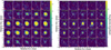 |
Fig. 6 High resolution channel maps of H2O (0,2,0) 65,2–74,3 transition at 268.149 GHz in R Hya and U Her. Each map (R Hya and U Her, left and right panels) shows offsets in the R.A. and Dec. directions which we call throughout this work “Relative RA” and “Relative Dec”. The corresponding angular offsets cover 100 × 100 mas from the continuum emission peak at (0,0) position (coordinates given in Table 1). Each channel velocity is in the LSR frame from −23.9 to 2.3 km s−1 (R Hya) and −28.6 to −2.3 km s−1 (U Her). White light contours are at −3, 3 and 5σ. A few negative contours, when present, are dashed. The line peak and typical rms noise are 65 and 1 mJy beam−1 (R Hya), and 122 and 1.5 mJy beam−1 (U Her). The red contour at (0,0) delineates the extent at half peak intensity of the continuum emission. We characterize the elliptical Gaussian clean beams by their major and minor axes and position angle (PA) at half power, hereafter HPBW clean beam parameters. For the line observations of R Hya and U Her, these are (38 × 29) mas at PA 48° and (26 × 19) mas at PA 11°, respectively. The corresponding continuum parameters are (34 × 25) mas at PA 67° for R Hya and (24 × 18) mas at PA 8° for U Her. The line and continuum beams are shown at the bottom left of each map in white and solid dark-red, respectively. The scale of the line flux density per beam (in mJy beam−1) is linear and shown in the vertical bar on the right side of each channel map. |
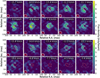 |
Fig. 7 High resolution channel maps of the (0,0,1) 31,3–22,0 and (0,2,0) 143,12–134,9 transitions of water near 254 GHz in R Hya. The upper and lower panels correspond tothe 254.040 GHz and 254.053 GHz transitions, respectively (lines 7 and 8 in Table 2). Caption as in Fig. 6 except for the velocity range and the line peak, 8 mJy/beam; the typical r.m.s. noise is 1 mJy/beam. The HPBW is (39 × 30) mas at PA 49° and (34 × 25) mas at PA 67° for the line and continuum, respectively. |
4.4 Absorption maps, comparison of absorbing/emitting regions
Figure 8 shows at 244.330 GHz the mom 0 absorption maps of R Hya, S Pav and R Aql obtained with spatial resolutions in the range ~35 mas (R Hya) to ~25 mas (S Pav, R Aql), together with the IRC+10011 mom 0 map obtained with ~55 mas resolution with the combined high and mid resolution arrays. Detection is at the 3–5σ level in front of the central star and is essentially unresolved even at our highest angular resolution.
We have also compared the 244.330 GHz absorption with the mom 0 maps of the emission/absorption of water at 259.952 GHz, and the mom 0 maps of the υ = 1, CO(2–1) emission/absorption at 228.439 GHz whose energy levels are close to those of the 259.952 GHz line. This is presented for R Hya in Fig. 9, left panel, where the υ = 1, CO(2–1) absorption coincides with the stellar continuum and the 259.952 GHz absorption of water. These absorptions are poorly resolved and coincide with the 244.330 GHz water absorption. The right panel in Fig. 9 shows that the 259.952 GHz water emission, which is slightly resolved, and the υ = 1, CO(2–1) emission (not shown here for clarity) have a comparable size, ~50 mas, as the 244.330 GHz water absorption.
The absorption feature observed in S Pav and R Hya between the two transitions of ortho H2O at 254.040 and 254.053 GHz (see spectra in Fig. B.4 and in upper right panel of Fig. 3 for R Hya) has also been mapped (Fig. D.14). Our mom 0 maps are sensitive enough to reveal spatially compact absorption structures with angular sizes as small as ~20–40 mas, or slightly more in R Hya, that are closely associated with the continuum emission from the central star. Such absorption features (see other examples in T Mic or R Aql (Fig. B.4) are redshifted by a few km s−1 with respect to the stellar systemic velocity and can be interpreted as being due to the presence of infalling matter (see Sect. 5.4).
4.5 Tracing the inner-wind regions at small scales
The majority of the H2O emission at 268.149 and 262.898 GHz, the two most widespread transitions, tends to show an organized “position versus velocity” structure in some stars. This is suggested in the channel maps where a slight displacement of the emission peak is present in different channels against the continuum emission source (e.g., 268.149 GHz line in R Hya and U Her, Fig. 6, or in IRC+10011, Fig. D.2). To better trace the deepest motions of the inner stellar wind, we have conducted a Gaussian analysis of the most compact, nondiffuse regions of water emission mapped in different transitions using the task SAD in AIPS9. The component fitting and sorting was performed here as in Etoka & Diamond (2004). We have used 5 times the rms noise level in the spectral channels as our typical threshold to extract components. We then built tables of velocity, line width and intensity components, applying additional criteria in terms of velocity and spatial “coherence” following the “maser feature” approach described in Sect. 2.2 of Richards et al. (2011). Maser emission usually has a genuinely Gaussian angular profile (e.g., Richards et al. 1999) and 2D Gaussian components can be fitted with accuracy determined by the S/N, as ~0.5–1×(beam/S/N). In theory the multiplier is 0.5 (see Condon 1997) but it can be greater (e.g., Richards et al. 1999). The accuracy is limited by deviations from a theoretical Gaussian and the dynamic range which can exceed 100 here; therefore, the lower limit to the errors is expected to be well below 1 mas. In practice, a component is deemed to be real if it is part of a spectral feature comprising at least 3 neighboring components with ~2 km s−1 velocity coherence.
Figure 10 presents examples od “position–velocity” maps of the various Gaussian-fitted velocity components identified in two prominent H2O sources. R Hya and U Her at 268.149 and 262.898 (3Hz. The fitted position uncertainty is reflected in the error bars of Fig. 10. In R Hya, both transitions show a quasi-linear poption-velocity structure ex tending along a SE-NW axis ~16 mas long across the 23.7 mas photosphere and well within the 27.1 mas radio continuum size measured at 250 GHz by Homan et al. (2021). On the other hand, the same two transitions in U Her show a more complex velocity field and a wider extent but again, with most of the blueshifted and redshifted components seen against the optical photosphere and the 250 GHz radio continuum disk (11.2 mas and 18.5 mas, respectively). For both stars, we know that any maser components seen in the direction of the star must be on the near side but we do not know directly the distance along the line of sight We do not exclude that an infalling gas clump on the far side of the sar’s limb overlaps an outflowing gas clump on the near side tor vice versa) but note that such cases would concern a small fraction of components, outside the line of sight to the radio continuum disk. The complex gas motions observed here, pointing to infall and outflow of gas, are consistent with other observations discussed later in Sect. 5.4.
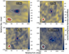 |
Fig. 8 Zeroth moment absorption maps of the (1,1,0)–(0,1,1) |

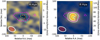 |
Fig. 9 Comparison of absorption and emission lines of water with υ = 1, CO(2–1) absorption in R Hya. Left: panel: Magenta and cyan dashed contours delineate the −5σ levels of the 244.330 GHz (line 5) and 259.952 GHz (line 10) mom 0 absorption maps. The underlying map is the mom 0 absorption map of υ = 1, CO(2−1) with the yellow dashet contour at the −3σ level. The line beam width is 550 × 28 mas with 70° orientation (white ellipse in bottom left corner The red solid contour delineates the 50% level of the peak continuum emission (the continuum beam width is the dark-red ellipse in the bottom left corner). Right panel: the magenta dashed contour and red solid contour indicate the 244.330 GHz absorption and mm-wave continuum emission as in the left panel. The underlying map is the 259.952 GHz mom 0 emission, with the white solid contours at the 20 and 35σ levels. (Line and continuum beam widths as in the left panel.) The noise level is 3 mJybeam−1 km s−1 for water in both panels and 4.3 mJy/beam km s−1 for CO. The velocity intervals of the mom 0 maps are: −13.2 to 4.3 and −2.3 to t.5 km s−1 for the 244.330 and 259.952 GHz absorptions; −18.8 to −3.0 km s−1 for the 259.952 GHz emission of water; −2.2 to 6.0 km s−1 for the CO(2−1) absorption. |
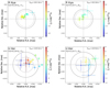 |
Fig. 10 Maps of the different velocity components of water identified in the Gaussian-fit procedure at 268.149 and 262.898 GHz toward R Hya and UHer for the extended configuration of the main array. The size of the colored symbols varies as the square root of the integrated flux density of the Gaussian component; the crosses show the position uncertainty for each component The velocity scale colors are given on the right side of each map with respect to the stellar system velocity taken to be −10.1 and −14.9 km s−1 in the LSR frame for R Hya and U Her, respectively. The dashed gray circle represents the size of the optical photosphere (23.7 and 11.2 mas for R Hya and U Her, respectively) and the larger gray circle represents the 250 GHz continuum emission size (27.1 and 188.5 mat for RHya and U Her). |
5 An initial H2O line analysis: Physical conditions
We derive here the H2O line brighlness temperature, the H2O column density and address questions related to the gas motion near the photosphere. Our calculations and discusston below are supported primarily by the H2O spectral data in Table 5 which reflect the diversity of physical conditionr in different sources for a given water transition and the diversity of the line excitation processes within a source.
5.1 Brightness temperature
Brightness temperature is an important quantity for qualifying the line excitation conditions. It is measured in two different ways. Firstly a good approximation to the brightness temperature, Tb, of compact sources is derived from the peak flux density per beam in our channel maps and the synthesized beam. The uncertainty in Tb il estimated from the typical noise in maps and the beam area. Our estimates are given in the last two columns of Table 6 for the two strongest water transitions, lines 12 and 14 at 262.898 and 268.149 GHz in υ2 = 1 and 2, respectively. The highest 268.149 GHz brightness temperature is ob served in U Her, VX Sgr, IRC+10011 and in AH Sco where Tb reaches 1.1 × 10⁶ K. The 262.898 GHz transition is not as strong as the 268.149 GHz transition reaching, however, 1.1 × 10³ K in IRC+10011. The above temperatures are lower limits to the actual brightness temperature for spatial components smaller than the beam size. Secondly, another approach to estimating the brightness temperature is provided by the de-convolved sizes of the Gaussian components fitted, as described in Sect. 4.5, to the 268.149 GHz features with a peak S /N ≳ 10. The calculated temperature, TGauss, is given in the second column of Table 6 and its uncertainty is estimated from the flux density error and the component size. TGauss is roughly 2.5 times larger than Tb derived from the channel maps for U Her and IRC+10011, and 8 times larger for AH Sco where it reaches 9 × 10⁶ K. These results indicate that the brightest 268.149 GHz emission features in these three stars are consistent with strong maser action.
Maximum brightness temperatures of ortho and para water at 268.149 and 262.898 GHz.
5.2 Population diagrams, opacity estimates
Our data provide only one pair of detected lines in the same vibrational state of the ortho H2O species (lines 8 and 14), and there is no similar line pair for the para species. Therefore, line intensity ratios derived from several transitions cannot be used to establish possible deviations from the LTE conditions (see also discussion in Sect. 6.3). However, an estimate of the excitation gas temperature and column density can be made from a population diagram (Goldsmith & Langer 1999) provided that the range of line energy used in such a diagram is large enough and that we are not too far from the optically thin case. (Deviations from the optically thin conditions could eventually be corrected at a later stage although this is uncertain as different transitions can have different opacities; such corrections are not attempted here.) We have constructed population diagrams for a few sources in our and para H2O) and does not separate the rotational from the vibrational partition functions for a better accuracy (Polyansky et al. 2018).
Examples of population diagrams for the observed ortho and para H2O emission lines are given in Fig. 11 using the high resolution data all observed within a few weeks and thus not affected by variability. In AH Sco and IRC+10011 we have excluded line number 14 which is masing (the corresponding data points lie well above the least squares line fit). Line 5 shows absorption only and is not used in our population diagrams. We derive Tex in the range ~1000–1500 K for all sources and column densities N(H2O) ~ 0.6, 2.2, 2.5 and 4.5 × 1020 cm−2 in AH Sco, R Hya, S Pav and IRC+10011, respectively. In R Aql where the dispersion of the data points is larger than in the other four sources we derive N(H2O) ~ 5.8 × 1020 cm−2. The uncertainty in the least squares fit slope may result in a temperature uncertainty as high as ~700 K at least (and higher in R Aql) but we note that, because the partition function varies monotonically with the temperature, this does not impact the estimate of the column density. The actual uncertainty in the projected density is difficult to evaluate, however. It is not very sensitive to uncertainties in the integrated line intensity used to derive N whereas the number of transitions and the range of energy covered in the population diagrams have an important impact. Discarding any line in the R Hya diagram for example, does not change significantly the N(H2O) estimates and, from random trials we suggest a statistical uncertainty of the column density at the level of ~25%.
The column density can be used to estimate the average water number density, provided the extent of the emission is known. In R Hya, the water emission has an extent of at least 3 times the continuum and from maps in different H2O transitions the likely depth of the water region is ~60–90 mas. At a distance of ~150 pc, the R Hya extent corresponds to 9–13 au which gives an average density of roughly (1.1–1.6) × 106 cm−3. For a fractional water abundance of 3 × 10⁻⁵ (used in Sect. 7) the H2 density is then (3.7–5.3) × 1010 cm−3 which is commensurate with the critical density derived in the next section. Our estimate of the H2 density in the inner regions of R Hya and in other sources remains uncertain, however, because of the difficulty in deriving a reliable emission water extent and since the H2O/H2 fractional abundance used here is debatable.
The opacity at the line center, τc, can be estimated from the quantity N/Q and the excitation temperature determined above, the energy of the transition and the observed line width. We derive τc ~ (5.145 × 10⁻⁴ × A21 ∫ n2dl)/(v2 × Δυ0 × T12) where v is in GHz for the transition from level 2 (upper) to 1 (lower), A21 the spontaneous emission rate in s−1, T12 the line excitation temperature, Δυ0 the line width at half intensity and ∫ n2dl the integrated density in cm−2. The latter quantity is obtained from the integrated Boltzmann population of the upper energy level using N/Q and T12 determined from the population diagrams. In R Hya, for example, we derive τc ~0.25, 0.3, 0.15 and 0.1 for lines 1, 10, 12 and 13, respectively. We point out that at 268.149 GHz (line 14) where maser excitation can be observed in some stars, our models indicate that negative opacities may become large (see Sect. 7). In R Hya, however, line 14 does not seem to be masing, or is not strongly masing, and we derive from our population diagram τc ~0.45 which is larger than the above opacities. In general, τc remains relatively small in other sources. However, for the low energy levels of line 10, we get τc ~0.4 in S Pav and even 0.75 in the thicker shell of IRC+10011.
Line 5 at 244.330 GHz shows only absorption which can be used to make another estimate of the gas opacity in the region where this line is excited. Toward R Hya, S Pav and R Aql, the absorption peak flux density reaches −8 to −10 mJy against the continuum source (Fig. 5) and the line excitation temperaiure must be below the continuum brightness temperature which, for Band 6 in R Hya, is ~2500 K (Homan et al. 2021). We derive τ244 ~0.015–0.08 for an excitation temperature close to gas temperatures in the range 1000–2000 K as predicted in moddls (o.g., Gobrecht et al. 2016). We also expect smalt opacities at 244.330 GHz in S Pav and R Aql for continuum and extitation temperatures similar to those in R Hya.
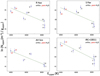 |
Fig. 11 Population diagrams for ortho and para H2O transitions (black and red numbers, respectively) in R Hya, S Pav, AH Sco and IRC+10011. The number near each data point corresponds to the numbering used to identify each line in Table 2. The vertical bar in each data point includes the ±1σ formal error of the integrated flux density and a rough estimate of the filling factor uncertainty. The green line is the regression line across the data points from which the rotationaf temperature and the column density are derived (see Sect. 5.2). The strong 268.149 GHz maser line (line 14) is excluded from the IRC+10011 and AH Sco plots while it is kept in R Hya and S Pav. |
5.3 Critical density
A full interpretation of all results in Table 5 requires a detailed modeling of water transititns up to the highest energy levels and is not attempted here (but see Sects. 6 and 7 for discussion on maser amplification). However, we can estimate for various H2O lines the critical density, nc, above which collisions with H2 dominate over spontsneous radiative de-excilation. This is done by comparing the spontaneous emisston rates and collision rate coefficients for all downward transitions connected to the upper level of the transition under consideration (see discustion in Faure & Josselin 2008). Adoptisg the collisional rate coefficients in Faure & Josselin (2008) for a range of different rotational transitions in, for example, the (0,1,0) vibrational state, we get nc ~5−2 × 1010 cm−3 for temperatures ~1000–4000 K, including the 658.007 GHz transition discussed in fett. 6.3. Another rough estimate for the widespread transitton at 268.149 GHz in the (0,2,0) vitrational state gives nc~1011 cm−3. These estimates and the H2 densities censidered in the chemistry models above the photosphere in regions ~ 1 – 10 R⋆ of typicail AGBs (e.g., Cherchneff 2006; Gobrecht et al. 2016) suggest that collisions become the prevalent excitation process in the post-shock gas layers where the rate of formation of water from OH is optimal. The above considerations cannot replace of course muttilevel radiative transfer models including exec( coltisional tates of water with H2. Such models are needed to explain supra-thermal excitation of water and why some water transitions are mesing in the circumstellar envetopes of AGBs (see Sect. 7).
5.4 Gas motion in the inner-wind region
The motion of circumstellar gas toward and beyond the photosphere of an evolved late-type star is the result of complex interactions between shock-driven pulsations, gravity and radiation pressute in the regions where new moleculss and dust grains are formed. Radial motions, even if they are dominant during the pulsation cycles of the central object. can be petiurbed by random motions within the inner-wind region or by gravitational interactions with a companion. Some of these questions are briefly discussed below in the light of our water line data.
In spite of a modest velocity resolution, the Gaussian component analysis of the most compact regions of water emission presented in Sect. 4.5 shows that an outflow or infall of gas can be traced in the 262.898 and 268.149 GHz lines. We find that the emission can be asymmetrically distributed around the central star and we observe velocity gradients or gas motions with an amplitude of several km s−1. An infall of matter toward the central star is directly suggested from our 244.330 GHz spectra which show a ~6–9 km s−1 redshift with respect to the systemic stellar velocities in R Hya, S Pav and R Aql (Fig. 5), and from the 244.330 GHz absorption maps in front of the same stars (Fig. 8). The gas infall interpretation is also strengthened by the inverse P Cygni profiles of the υ = 1, CO(2−1) transition in R Hya, S Pav and R Aql (Fig. 5) and by line maps showing a close spatial association of the CO and water molecular species within a few stellar radii (Fig. 9). We further note that inverse P Cygni profiles similar to our CO(2−1) profiles have been observed with ALMA in υ = 1, CO(3−2) toward R Aqrand R Scl by Khouri et al. (2016) who concluded that the gas falls on these objects within ≲3 R⋆ with a velocity of 7–8 km s−1 (and a dispersion of 4 km s−1). They also derived, in the molecular layers before the wind starts, densities on the order of a few 1010 cm−3 to ~4 × 1011 cm−3 which are comparable to or above the critical density estimated in Sect. 5.3. Infall velocities of ~5–10 km s−1 magnitude estimated from our water and CO radio line observations, and from the CO lines in Khouri et al. (2016) are close to model predictions. In particular, the models developed by Nowotny et al. (2010) to synthesize the observed CO or CN infrared line profiles and to match the velocity variations observed in the dust-free ~1–2 R⋆ region of AGBs require infall/outflow velocities of ~5–10 km s−1. Motions of deeper and pulsating gas layers were studied from the CO near-infrared overtone bands (e.g., Hinkle et al. 1984). We also point out that in complex stellar systems, such as the symbiotic star R Aqr, the gas motions are affected by the presence of the stellar companion (e.g., Bujarrabal et al. 2013).
The water line velocity of the peak emission extracted from the observations provides an estimate of the systemic stellar velocity but little information on the atmospheric dynamics. To tentatively compare the observed radial velocity information with models we use the total velocity range between the red and blue extremes of each line, Δν, as defined in Sect. 2.2 and given in Table 5. We first point out that in most cases the emission at extreme velocities is within 0.′′04 of the star and thus, using for spectra an extraction aperture diameter larger than 0.′′08 would not change Δυ significantly; in fact, similar Δυ is usually measured in an aperture half that size. Occasionally, a smaller Δυ can be measured from a larger aperture or from lower resolution data, which must be due to beam dilution or imaging artifacts, including absorption which sometimes occurs, or, if considering mid resolution data, due to the lower sensitivity of these data. Examination of the channel maps resolves these apparent issues. Using Table 5, we find that for each detected transition and for each star, Δυ is always ≳5 km s−1 and may reach ~15–30 km s−1 at 268.149 GHz with the highest values in the supergiants AH Sco and VX Sgr. Assuming that the line profiles are grossly symmetric about the stellar velocity and that the velocity fields are not strongly asymmetric, the maximum outflow/infall velocity can be estimated from 0.5 × Δυ which gives ≲12 km s−1 in AGBs and ≲13–15 km s−1 in AH Sco and VX Sgr. Another way to estimate the outflow and infall velocities is to take the most blueshifted and redshifted velocities of the water lines as defined in Sect. 2.2 to determine the velocity extent. These velocities vary with the star and the line being examined (the 268.149 GHz transition often gives the largest velocities). Overall, the range of outflow and infall velocities covers around –(3–15) and (2–15) km s−1, respectively; there is no clear difference between the AGB stars and AH Sco and VX Sgr. These outflow/infall velocities are in accord with the radial pulsation modes described in the nonlinear models of Ireland et al. (2011, predicting expansion velocities at such velocities and shocks propagating even faster), and with the maximum velocity of ~10 km s−1 used in the AGB models of Bladh et al. (2019). Comparing the observations with models remains uncertain, however. We note that, in addition to sensitivity limitations, an observed narrow velocity range, for example, could be due to the clumpy and irregular nature of the mass loss phenomenon that we are sampling. The larger values of Δυ could also be influenced by interactions with a companion (see below).
In a few stars the blue and red wing line velocities of the 268.149 GHz spectra exceed the υ = 0, CO(2−1) line wings although, as shown in Gottlieb et al. (2022), the ATOMIUM observations provide high sensitivity to low level CO emission. Such a comparison may, however, still be hampered by the dependence of the CO velocity range on sensitivity and by the fact that the interpretation of the 268.149 GHz line profile may be complicated by maser action (e.g., variable pumping and beaming conditions over a given region may give rise to asymmetric line wings). Nevertheless, we observe that, for the high resolution data, the 268.149 GHz water line wing emission exceeds that of CO(2−1) in RW Sco, T Mic, U Her, AH Sco and R Aql. (In the latter source both the red and blue water line wing velocities exceed the CO(2−1) emission.) This finding is reminiscent of weak υ = 1, SiO(2−1) maser features observed by Cernicharo et al. (1997) and Herpin et al. (1998) at velocities exceeding the υ = 0, CO(2−1) velocity range. The high velocity emission of water reported here could be explained in different ways, including rotation, asymmetrical gas expansion (potentially explaining blueshifted components in front of the star, if observed), turbulence or kinematic perturbations by a companion. The surface rotational velocities of evolved stars are expected to be small although models (e.g., Ireland et al. 2011) consider that the stellar surface velocities can reach ~10–20 km s−1. Slow surface rotation is observed indeed in R Dor for which Vlemmings et al. (2018) suggest a probable acceleration by a nearby companion and, in Betelgeuse and its close envelope which exhibit a slow equatorial velocity of a few km s−1 (Kervella et al. 2018). The high velocity emission present in our data is most probably due to the impact of a stellar or planetary companion on the local gravity and/or to the complex and irregular nature of the inner wind where the 268.149 GHz line of water is excited. Binarity, depending on the mass ratio and other model parameters, was shown to be dominant in shaping the wind of the AGB stars and RSGs and can lead to a high speed emission of the gas close to the star out to a hundred or more stellar radii (Decin et al. 2020; Gottlieb et al. 2022)10.
6 Widespread emission at 262.898 and 268.149 GHz
Lines 12 and 14 at 262.898 and 268.149 GHz in the vibrational states (0,1,0) and (0,2,0) are the two strongest and most widespread transitions in this work (see Table 5 and Appendix B). Their line peak and line profile variability are discussed below.
Dates of observations with the main and ACA arrays and associated optical phases (in parentheses) of the variable 268.149 GHz H2O sources.
6.1 Time variability
Time variability in any of the circumstellar water lines observed here, once demonstrated, suggests changing physical conditions. In the pulsating and shocked environment of the ATOMIUM O-rich stars we expect indeed changing line excitation conditions and, hence, some variations in the water line peak intensity and/or profile. In weak lines, however, small deviations from the quasi-LTE excitation conditions may be difficult to demonstrate. Nevertheless, based on their integrated line intensity measurements in υ2 = 1 and 2 transitions of water, Velilla-Prieto et al. (2017) reported tentative line variability in IK Tau. We point out that while variations with quasi-LTE excitation conditions are difficult to prove, variations with maser-type excitation conditions may be easier to identify. In masers, time variability of the line emission peak and profile become more probable since changing physical conditions in the circumstellar gas may result in amplified variations of the stimulated emission, provided that the line is not highly saturated. (Analysis of the molecular light polarization would also help to characterize any maser action; this is not possible here and would deserve dedicated observations with ALMA or other facilities.)
6.1.1 268.149 GHz line variability
There is no systematic monitoring of the 268.149 GHz line emission in this work. However, time variability can be addressed by comparing the mid- and extended-configuration spectra of the main array obtained at two different epochs and for the same 0.″4 aperture diameter. We observe markedly different peak flux density ratios at the two epochs of the observations in U Her, GY Aql and the two RSGs AH Sco and VX Sgr (Table 7) and there is a secondary line feature near −17.1 km s−1 in U Her (Fig. 12). Table 7 gives the dates and optical phases of the observations together with the ratio of the mid to extended peak flux density ratio. RW Sco is added to Table 7 despite the peak flux density ratio is equal to one because the line shape is very different at the two epochs of the main array observations. The ACA observations of GY Aql and R Aql, also summarized in Table 7, are presented later in this section.
Variability toward U Her is the most accurately documented case because a similar mid configuration of the main array antennas was used in both October 2018 and August 2019. Comparing the spectra at these two epochs (corresponding to the optical phases ∼0.13 and ∼0.92), the peak flux changed by a factor of ∼24 (Fig. 12). In addition, despite our modest ∼1.1 km s−1 resolution, the stronger emission spectrum of 2018 exhibits a secondary feature around −18 km s−1 next to the main line emission suggesting multicomponent excitation. Spectral narrowing of the main line feature is discussed in Sect. 6.2. There is also a clear difference in the angular extent of the 268.149 GHz emission observed in October 2018 and August 2019 as shown in our zeroth moment maps (Fig. 14). The area within the 5σ contour of the emission in October 2018 is typically ∼3.5 times greater than the area within the 5σ contour in August 2019 when the emission was weaker. (There is still the possibility, however, that these two different mid-configurations of the array are not equally sensitive to extended weak components.) In addition, Fig. 14 shows an emission blob at the SW of the main source in the October 2018 data when the emission activity is greater11.
Our 2021 ACA observations of GY Aql and R Aql provide an additional epoch to assess the variability of the 268.149 GHz line emission in these two sources. To support the idea that the ACA and ATOMIUM main array data can be compared, we have extracted spectra for these two sets of data using different circular apertures encompassing all detected emission. The ACA spectral windows include (see Sect. 2.3), in addition to H2O lines and to the probably masing υ = 1, 29SiO(6−5) transition, two relatively strong transitions of υ = 0, HCN(3−2) and ν = 0, SO(56−45) at 265.886 and 251.826 GHz, respectively. We find that the ACA and mid configuration line profiles and peak flux densities in HCN and SO of both GY Aql and R Aql are nearly identical, thus demonstrating that the ACA can recover the same total emission as the mid configuration of the main array. A similar conclusion is obtained for GY Aql in the ν = 0, SiS(14−13) line at 254.103 GHz. We have thus used these results to compare the 268.149 GHz line emission spectra from the ACA and the mid and extended configuration (Fig. 15). In GY Aql, the 268.149 GHz line was only barely detected by the ACA at optical phase 0.8 (Table 7). The 3σ level flux density, 72 ± 24 mJy at ∼32 km s−1, is significantly weaker than our detection with the extended configuration in July 2019 at the optical phase of ∼0.2.
This line was buried in the noise of the mid-configuration observations in November 2018 at the optical phase of ∼0.7 very close to that of our ACA observations. In R Aql (Fig. 15), the ACA peak emission at the optical phase of 0.2 (Table 7) is stronger than the mid and extended configuration peak emission at the optical phases of ∼0.4 and 0.2, respectively; the spectrum also peaks at a slightly different LSR velocity.
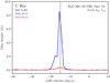 |
Fig. 12 Comparison of the 268.149 GHz line profiles in U Her observed with the mid configuration of the main array in Oct 2018 and Aug 2019 (blue and red curves, respectively). The spactra are extracted for an aperture diameter of 0.″4; the Spectral resolution is ∼1 km s−1. The vertical line shows the systemic stellar velocity. The mom 0 emission maps at these two epochs are presented in Fig. 14. |
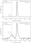 |
Fig. 13 Comparison of the 268.149 GHz line profiles extracted for an aperture diameter of 0.″4 in VX Sgr observed at ∼1 km s−1 resolution in November 2018 and July 2019 with the mid and extended configurations of the main array (upper and lower panels, respectively). The weak feature near −20 km s−1 in the 2019 spectrum corresponds to the ν = 0, JKa,Kc = 95,5−104,6 transition oO SO2 at 268168.335 MHz; it is also barely seen in the 2018 mid spectrum. The vertical lines are at the adopted new LSR systemic velocity. |
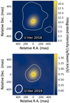 |
Fig. 14 Zeroth moment maps of the 268.149 GHz emission of water in U Her obtained with the mid configuration of the main array at two different epochs, 2018, Oct. 14 and 2019, Aug. 24. The emission is integrated over the −21.6 to −9 km s−1 velocity range. The 2019 image has been convolved with the larger 2018 image beam shown in the lower lrft of each panel (0.″21 × 0.″18). In both maps the noise is 0.02 Jy beam−1 km s−1 and the 5σ emission contour is shown as a white light: contour. The map maxima are 21.6 and 1.67 Jybeam−1 km s−1 in 2018 and 2019), respectively. The small red contour at the image center is the 50% continuum emission from the high resolution data. Note the SW blob emission in the 2018 map (see Sect. 6.1.1). |
6.1.2 262.898 GHz line variability
There is no clear evidence of time variability in the ATOMIUM data at 262.898 GHz (line 12) when we compare the peak line flux density of detected sources at different epochs. In addition, the line 12 profiles show a dominant quasithermal line excitation in agreement with our population diagram results in Sect. 5.2. However, toward IRC+10011, a close examination of the spectra acquired with the extended, mid and compact configurations of the main array at different dates (observations of June, Aug. 2019 and Dec. 2018) shows a time-varying emission where the line flux density has changed by a factor of ∼2 over the time span of half a year (Fig. 16). This result suggests that even though thermal emission dominates in the line 12 profile, some maserlike emission may also coexist in our data. Maser models show indeed that there are favorable conditions in the stellar environment to invert the line 12 population levels in the υ2 = 1 state (see Sects. 6.4 and 7).
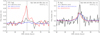 |
Fig. 15 Comparison of the 268.149 GHz line profiles in GY Aq1 and R Aql observed with the ACA and the mid and extended main array configurations. The ACA spectral resolution has been degraded here to 2 and 0.5 km s−1 (GY Aql and R Aql, respectively) for comparison with the ~1 km s−1 resolution of the mid and extended configurations of the main array. The epoch of the observations are indicated in the figure labels as well as the diameter of the extraction aperture given in parentheses (18.″0, 0.″4 and 0.″2 for GY Aql and 18.″0, 1.″0 and 0.″1 for R Aql). The vertical lines show the systemic stellar velocity. |
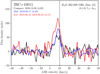 |
Fig. 16 Comparison of the 262.898 GHz line profiles in IRC+10011 observed at different epochs with the mid, extended and compact configurations of the main array. The epoch of the observations and the diameter of the extraction apertures (4″.0, 0″.4 and 0″.15) are shown in the figure labels. The spectral resolution is ~1.1 km s−1. The vertical line shows the systemic stellar velocity. |
6.2 Line narrowing at 268.149 GHz
In addition to 268.149 GHz intensity variations in U Har and VX Sgr (Figs. 12 and 13), we have observed a clear narrowing of the full width at half maximum, by a factor of ∼2, when the line is stronger. There is no direct evidence of significant fine narrowing in other targets, including AH Sco the strongest 268.149 GHz source which shows similah narrow fine widths at the time of the 2018 and 2019 observations. In U Her (Fige 12), accounting for the 1.1 km s−1 instrumental line broadening, the intrinsic line width of the main 268.149 GHz spectral component is around 4.3 and 2.0 lern s−1 in Aug. 2019 and Oct. 2018, respectively. When the emission is stronger (Oct. 2018), the narrowed line width is comparable but slightly below the 2.0−9.5 km s−1 Doppler line width derived for akinetic temperature in the range ∼ 1500 to 2500 K. Such a line narrowing suggests maser action in an unsaturated maser. However, since a discussion of maser saturation is impossible with our ATOMIUM data atone, an estimate of the 268.149 GHz opacity at the line center from these fine widths is uncertain, fin VX Sgr (Fig. 13), the observed line widths as half antensity, corrected for instrumental broadening, are ∼3.7 and 6.4 km s−1 at the time of the stronger (2018) and weaker (2019) emission, respectively. Such fine widths are broader than the expected thermal line profiles and likely to be blends of emission from individual H2O clumps along the line of sight due to the velocity gradients in the circumstellar material.
To indirectly identify a posaible sign of 268.149 GHz line narrowing in unsaturated masers despite our moderate spectral resolution, we have compared the fine width at hals intensity of this transition with other waler sines in the same source This approach is limited, however, since line widths alone cannot be used to prove or disprove maser action and the conditions leading to fine rebroadening or inhibiting line broadening of saturated masers are difficult to assess. Nevertheles, in addition to U Her and VX Sgr discussed above, we observe that the 268149 GHz line widths lie in the range ∼2.0−4.5 km s−1 toward AH sco, IRC+10011, IRC−10029, RW Sco, GY Aql, and R Aql while other detected water transitons are generally broaden In AH Sco, for example, the fine width is ∼2.5 km s−1 at 268.149 GHz and ∼5−7 km s−1 in all other water transitions. On the other hand, V PsA and R Hya do not exhibit narrow 268.149 GHz fine profites (∼ 14.5 and 8.5 km s−1 at half intensity, respectively) and in R Hya our population diagram (Fig. 11) shows that there is no strong deviation from LTE (and hence no dominant maser amplification in this source). An additional sign of maser action is provided if a secondary narrow spectral feature is identified. This is observed in the 268.149 GHz spectra of GY Aql, U Her and S Pav near 38.1, −17.1 and −6.7 km s−1, respectively, without any apparent confusion with other molecular transitions. Maser lines can be narrower than 1 km s−1, so, together with the extended array, a higher spectral resolution would be desirable to reveal the presence of multiple unresolved spectral components as suggested by the asymmetrical 268.149 GHz line profile in S Pav.
6.3 268.149 GHz line excitation
The (0,2,0) 65,2−74,3 transition of water at 268.149 GHz is widespread in evolved stars since it is observed in 15 out of the 17 objects of the ATOMIUM sample to which one must add three other sources not included in our sample, VY CMa with strong emission first reported by Tenenbaum et al. (2010), IK Tau with weak emission first mentioned by Velilla-Prieto et al. (2017) and W Hya with strong maser emission recently reported by Ohnaka et al. (in prep.). In VY CMa, the line peak flux density reached ∼650 Jy which suggests strong maser amplification. In all sources of the ATOMIUM sample the 268.149 GHz transition is always the strongest water line (see Table 5) and, in AH Sco and IRC+10011, the observed peak flux density reaches ∼70 and 2 Jy at the epoch of the observations. The brightness temperature, Tb, derived from the peak flux density in our channel maps is ≳1−6 × 10³ K and reaches ∼4.4 × 10⁴ K and 1.1 × 10⁶ K in IRC+10011 and AH Sco, respectively (Table 6). Even higher values of Tb are obtained in these two stars and in U Her from the Gaussian component analysis described in Sect. 4.5. Such high brightness temperatures indicate maser-type amplification of the 268.149 GHz emission since they are greater than the expected kinetic temperature in the preshock or postshock inner gas layers where this line is excited. A trend toward non-LTE conditions is also suggested from the ratio of the peak flux densities at 268.149 and 254.053 GHz, S268/S254. Both transitions lie in the same (0,2,0) vibrational state and their LTE line opacity ratio, (τ268/τ254)LTE, is ∼0.9 for an excitation temperature of ∼300 K. The exact line excitation temperature and opacity of the observed lines are not modeled here but we point out that the observed flux density ratio, S268/S254, is well above the LTE opacity ratio. Based on the values in Table 5, we derive S268/S254 in the range ∼5 (IRC−10529) to ∼140 (IRC+10011), and even much higher in AH Sco where the 254.053 GHz transition is not detected. This suggests that, in general, thermal excitation is not the dominant line excitation process at 268.149 GHz.
From these remarks and our discussion in Sects. 6.1 and 6.2 we conclude that the widespread 268.149 GHz emission observed in evolved O-rich stars tends to be time-variable (e.g., U Her) and masing (e.g., AH Sco) even though quasi LTE line excitation conditions are also observed in some sources (see R Hya and S Pav population diagrams where including line 14 is relevant, Fig. 11).
H2O line modeling (see Sect. 7) and any correlation of the 268.149 GHz line parameters with other vibrationally excited H2O lines add new insights into the understanding of the nature of the 268.149 GHz emission. In particular, we note that eight of the fifteen 268.149 GHz sources of ortho H2O in Table 5, T Mic, RW Sco, R Hya, U Her, AH Sco, R Aql, IRC+10011, VX Sgr, also exhibit emission of the same water species in the most widespread (0,1,0) 11,0−10,1 transition of H2O at 658.007 GHz (Menten & Young 1995; Hunter et al. 2007; Justtanont et al. 2012; Baudry et al. 2018b,a)12. Although both transitions are not in the same vibrational state, and despite time variability may hide any potential relationship between these two lines, the brightest sources at 268.149 GHz tend to show strong emission at 658.007 GHz. The 658.007 GHz transition has a clear tendency to be masing with minimum brightness temperatures Tb(658) ∼104−10 K for those sources also exhibiting 22.235 GHz masers (Baudry et al. 2018b). The latter work and Menten & Young (1995) also showed from a comparison of the velocity ranges of the 658.007 GHz and SiO(2−1) maser emissions that the 658.007 GHz transition is excited within or close to the SiO maser-emitting region, that is ∼5 R⋆.
Interferometric observations at 658.007 GHz were performed by Hunter et al. (2007), but direct demonstration that this line can be inverted comes from the ALMA observations of the RSG VY CMa (Richards et al. 2014) indicating compact, Tb ∼ 0.3−4 × 10⁷ K components, that is roughly consistent with a spherical shell13. Mapping of AGBs is not available yet at 658.007 GHz, but this line is currently known to be excited in about 60 evolved objects according to our source count and latest 658.007 GHz observations (Baudry et al. 2018a). Since eight of the ATOMIUM sources are also known 658.007 GHz emitters and, because of the relatively large number of identified 658.007 GHz sources, the actual number of 268.149 GHz stellar sources is likely to be larger than reported in the present work. The general physical conditions leading to 268.149 and/or 658.007 GHz maser emission are discussed further in Sect. 7.
6.4 262.898 GHz line excitation
The (0,1,0) 77,4−86,2 transition of para H2O (line 12 in Table 2), is the only rotational transition covered in our observations that arises from the lowest vibrationally excited state of H2O in the υ2 = 1 bending mode. Although this line is weaker than the 268.149 GHz transition, the detection rate of both transitions is comparable (12 and 15 objects, respectively, see Table 5). In contrast with the 268.149 GHz line which may show strong maser radiation in some sources, examination of the 262.898 GHz line profiles and the population diagrams in Fig. 11 suggest that line 12 does not exhibit strong non-LTE characteristics. This does not imply, however, that population inversion is impossible as indicated by time variability of some 262.898 GHz spectral features in IRC+10011 (see Sect. 6.1.2), and by the general maser line amplification discussion in Sect. 7.2.
Rotational transitions within the (0,1,0) state are nearly always observed toward evolved stars14 and, if the (0,1,0) 77,1−86,2 line of para H2O is excited at 262.898 GHz, then one will almost always detect one or more H2O lines from the (0,1,0) state. This is supported by ground-based observations of late-type stars at: 658.007 GHz (see discussion in the previous section); 96.261 and 232.687 GHz in VY CMa and W Hya (Menten & Melnick 1989) and, at 232.687 GHz, in VY CMa with ALMA (Quintana-Lacaci et al. 2023); 293.664, 297.439, and 336.228 GHz in VY CMa (Menten et al. 2006; Kaminski et al. 2013) and 336.228 GHz in R Dor and IK Tau (Decin et al. 2018); 232.687 and 263.451 GHz in RS Cnc (Winters et al. 2022). In addition, several υ2 =1 lines have been observed with Herschel/HIFI in various AGB stars and supergiants/hypergiants (Justtanont et al. 2012; Teyssier et al. 2012; Alcolea et al. 2013).
Except for the (0,1,0) 52,3−61,6 line at 336.228 GHz, all transitions observed in the υ2 = 1 state have an upper level with Ka = J and Kc = 0 or 1, including the strong 658.007 GHz line. In parallel with the terminology of “backbone” levels used by de Jong (1973) in his overpopulation model of the J = Kc levels and in his 22.235 GHz ground state maser model, Alcolea & Menten (1993) referred to the J = Ka upper levels as on the “transposed backbone” and proposed a pumping mechanism that results in a systematic overpopulation of these levels within the υ2 = 1 state. They found that, following collisional pumping to the υ2 = 1 state, some infrared radiative decay routes of these transposed backbone levels to the ground state become more optically thick than the lower, nonbackbone levels for gas density, kinetic temperature and H2O column densities typical of the inner circumstellar envelopes. This tends to reduce the radiative decay rates of the levels on the transposed backbone and, hence, results in a systematic overpopulation compared to that in the lower levels. Predicting the efficiency of this mechanism was not possible, however, on the basis of the uncertain collision rates and LVG (large velocity gradient) modeling approximation used in Alcolea & Menten (1993).
It is interesting to note that the ortho H2O counterpart of the para H2O line at 262.898 GHz (line 12), the (0,1,0) 77,0−86,3 line at 263.451 GHz (not covered in our frequency setup) has been detected in a few evolved stars. The 263.451 GHz ortho line was first mentioned by Alcolea & Menten (1993) without presenting the spectrum. An emission line at 263.452 GHz was also detected in the line survey of IK Tau by Velilla-Prieto et al. (2017), but the carrier was not identified. Recently, Winters et al. (2022) observed this line in the MS-type AGB star RS Cnc. Modeling of the 262.898 and 263.451 GHz line pair and other line pairs in the (0,1,0) vibrational state are discussed in Sect. 7.2.
7 H2O maser models
7.1 General comments
Competition between radiative excitation and de-excitation of many H2O levels together with collisional excitation and de-excitation of H2O with H2, H and/or electrons15 may result in a population inversion of various energy levels of water and, eventually, lead to a predominant stimulated emission of radiation in specific transitions; a stimulated emission rate greater than the absorption rate is the prime condition to trigger an astro-physical maser. Population inversion is facilitated in molecules such as water because it has many levels of similar energy (e.g., the 61,6 and 52,3 rotational levels in the ground vibrational state giving rise to the emblematic 22.235 GHz maser emission). Therefore, any radiative transfer model of water must take into account potential inversions of the water line levels. Multilevel calculations up to energies ∼7000 K in the ground vibrational state were first presented by Neufeld & Melnick (1991) to model the 22.235 GHz maser and predict several other collisionally pumped maser lines throughout the energy ladder. Later, Yates et al. (1997) identified radiatively pumped lines of water and showed that dust radiation tends to weaken the collisionally pumped maser lines in the (0,0,0) vibrational ground state. Sensitivity to the dust temperature of maser lines in the (0,0,0) state is also observed in Bergman & Humphreys (2020). Other models have explored the impact of different collision rates on the maser line opacities (e.g., Daniel & Cernicharo 2013) and, recently, Neufeld et al. (2021) used their collisional pumping models to explain the observation of new THz water lines in the (0,0,0) state toward evolved stars. Infrared radiative pumping in the (0,1,0) vibrational state by hot dust was first considered by Goldreich & Kwan (1974) and, most recently, Gray et al. (2022) have shown that radiative pumping to the (0,1,0) state can also explain the 22.235 GHz maser in the low kinetic temperature regime and at high dust temperatures.
7.2 Highly excited water masers
Extensive modeling of water masers was presented in Gray et al. (2016) who predict maser emission in evolved stars for many observable transitions. Their models process 411 and 413 levels of ortho and para H2O distributed across the first two excited states of the bending mode, (0,1,0) and (0,2,0), the first excited state of both stretching modes, (1,0,0) and (0,0,1), as well as the ground vibrational state. Line overlap effects within the ortho and para water transitions are also considered separately in the two species16. The large number of slab-geometry model outputs allows us to explore a large parameter space in density, nH2, kinetic temperature, TK, and dust temperature, Tdust. It was found that the maser transitions can be divided into three main groups: one exhibiting both radiative and collisional pumping, one with dominant collisions, and another group with a dominant radiative pumping component. The 268.149 GHz maser emission in the (0,2,0) state pertains to the latter group when Tdust is high (Sect. 7.2.1).
We reexamine below the maser slab model outputs to better understand the excitation of the three strongest and most widespread water lines observed in this work, lines 10, 12 and 14 at 259.952, 262.898 and 268.149 GHz (see Table 5). We have three main goals in mind: (i) explore if there are favorable physical conditions for the cospatial excitation of the strong 268.149 and 658.007 GHz lines as suggested in Sect. 6.3; (ii) investigate the conditions leading to the relatively strong line emission observed at 262.898 GHz (this work) and in other υ2 = 1 lines (see references to other published works in Sect. 6.4), and (iii) assess the conditions leading to significant excitation of the 259.952 GHz line in the ground vibrational state. Ortho and para H2O are treated separately and the H2 abundance is obtained from the H2O abundance divided by the fractional abundance of H2O/H2 = 3 × 10⁻⁵ that is considered in our models.
7.2.1 268.149 GHz
We find that for the high density conditions favorable to masers, the 268.149 GHz transition is weakly, or not inverted at kinetic temperatures ≳500 K for Tdust in the range ∼50 K to a few hundreds K. When Tdust reaches several hundreds or ≳1000 K, 268.149 GHz inversion tends to move to higher values of TK in the density vs. kinetic temperature plane. Increasing Tdust from 900 to 1300 K, for example, increases the inversion as shown in the upper two panels of Fig. 17 for TK ≲ 500 K and ≲900 K, respectively, around  . Inversion i thus expected dor nH2 ∼3 × 10⁹−3 × 1010 cm−3 and for Tdust = 900 and 1300 K. Within She inner 3−10 R⋆ region where we observe the 268.149 GHz line and where the dust has just formed and is optically thin, the radiation field is dominated by the central star and we expect indeed high Oust temperaiures and densities.
Οn the other hand, the radiative pumping component, needed for the 268.149 GHz maser, is not needed at 658.007 GHz for which lower values of Tdust (≲800 K) tend to provide strong inverrion for a broad rangt of TK (see lower two panels in Fig. 17). Thefefore, the physical canditions prevailing within the inner gas layers where we expect high Tdust do not seem a priori favorable to the 658.007 GHz maser excitation. High Tdust conditions may nevertheless result in 658.007 GHz line inversion if TK ≳ 3000 K (see lower left panel of Fig. 17) which is plausible in the shocked environment of the expanding stars but, in turn, is not favorable to 2(68.149 GHz line inversion. We can not exclude, however, that in some peculiar objects, tooler and less dense conditions than required for 268.149 GHz are favorable to the 658.007 GHz maser. We note that in VY CMa, the 658.007 GHz masers (Richards et al. 2014; Asaki et al. 2020) are mostly located at roughly twice the distance from the star where the SiO masers are observed, supporting slightly cooler confirions favorable to the 658.007 GHz line excitation, possibly once opaque dust has formed. (Alternatively, these 658.007 GHz masers could- also be excited by a shock around the VY CMa clump C.)
We conclude that in general, excluding the peculiar VY CMa object, the potential link between the 268.149 and the 658.007 GHz line emissions mentioned earlier in Sect. 6.3 (on the basis of source detection rates) is not straightforwardly explained in terms of our current maser models. Of course both lines are not necessarily masing at the same time and position in a same object, and a possible relation between observed lines may be more difficult to decipher than with a simple search for common masing conditions
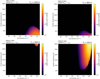 |
Fig. 17 Comparison of maser depths of ortho H2O at 268.149 and 658.007 GHz (upper and lower two panels) using models in Gray et al. (2016). Strong maser emission at 268.149 and 658.007 GHz is obtained for markedly different kinetic temperatures (vertical axis on left hand-side of each panel) and dust temperatures Td (given in the upper right-hand side of each panel). The transition frequency is given in the upper left corner of each panel with, below the letter o for ortho H2Ο followed by the vibrational stale fnd the rotational transition. The negative optical depth is specified in the vertical bar on the right-hand side of each panel using a log normal scale (min = −0.1 and max = −75.0); black means no inversion. The molecular H2 density is obtained by dividing the water abundance by 3 × 10⁻⁵.) |
7.2.2 262.898 GHz
We mention at the end of Sect. 6.4 the importance the differential radiative trapping scheme for the J = Ka “transposed backbone” levels in the (0,1,0) state. Especially for the para and ortho H2O line pair at 2(52.898 (our widespread line 12) and 263.451 GHz observed by Winters et al. (2022, see Sect. 6.4 and below). Our models demonstrate that both lines can be masing but for different physical conditions. Line 12 remains a weak maser in the TK versus density regions considered here for both low and high dust temperatures (~50 and ≳1000 K). We find, for example, that the dominant route for population inversion at 262.898 GHz for Tdust = 1025 Κ and  , requires TK ≳, 2300 Κ (see the weak negative opacity contours at 262.90 GHz in the top right-hand corner of the upper panel in Fig. 18) in contrast with the lower TK ≳ 700 Κ required at 263.451 GHz (bottom right corner of the 263.45 GHz maser plot in the lower panel of Fig. 18). Our model outputs can be compared with the observations of the 262.898 and 263.45 GHz line pair. At 262.898 GHz, the brightness temperature derived from the ATOMIUM data do not give unambiguous evidence of masing (Table 6) but this could be due to the emission being very compact so that the measured temperature is a lower limit. In addition, the 262.898 GHz line profiles are narrow and there is some evidence for variability (Sect. 6.1.2 and Fig. 16). We conclude that this transition could be weakly masing in the inner gas layers with high density and high kinetic temperature. Our models also predict 262.898 GHz inversion over a wide range of dust temperature from ~100 to ≳1000 Κ and for
  and TK ≳ 2000 K. For the ortho H2O line at 263.451 GHz, the line profile in RS Cnc appears to be rather broad and stable (Winters et al. 2022). Similarly, the unidentified emission feature in IK Tau at the same frequency (Velilla-Prieto et al. 2017), which we identify as the ortho H2O line, does not show obvious signs of maser action in its line profile. Observations of other stars should be performed to characterize this emission, but we momentarily conclude that the maser conditions quoted above for the 262.898 GHz transition do not apply to the 263.451 GHz line (see Fig. 18 for Tdust ~ 1000 K). We also note that the low TK, high H2O density regime of these two lines do not exactly overlap (Fig. 18)17.
Finally, we draw attention to a rather rare occurrence in our models. The upper panel in Fig. 18 at 262.898 GHz shows that both radiative and collisional pumping regimes can coexist at the same dust temperature whereas most transitions that have both schemes show a clear bifurcation at Tdust ~750−1100 Κ where the dominant pumping route switches from collisional to radiative. This two-inversion occurrence although seen faintly here at 262.898 GHz can be stronger in a few other maser lines (e.g., at 209.118 and 96.261 GHz).
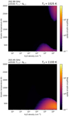 |
Fig. 18 Negative optical depths as in Fig. 17 at 262.898 and 263.451 in the (010) vibrational state. The quantum numbers of these transitions are preceded by the letters ρ and ο for para and ortho H20. (The molecular H2 density is obtained by dividing the water abundance by 3 × 10⁻⁵.) |
7.2.3 259.952 GHz
We have not observed any clear sign of time variability in our data at 259.952 GHz (line 10) in the ground vibrational state. However, variability may be hidden by the limited number of epochs available to us in the ATOMIUM program. Line 10 is weaker than the 262.898 and 268.149 GHz lines (lines 12 and 14) but it is usually stronger than all the other lines (Table 5). We find that line 10 has a relatively strong radiative pumping component for conditions reminiscent of those modeled for the 268.149 GHz maser. This is seen by comparing the 260 GHz plot in Fig. 7 of Gray et al. (2016) at a dust temperature of 1025 K, with the upper panels of our Fig. 17 at 268.149 GHz. Line 10 can thus be weakly inverted close to the photosphere but, in contrast with the strong 268.149 GHz emission, it does not show strong signs of maser emission.
We conclude Sect. 7.2 by stressing that observations toward more evolved stars in the υ2 = 1 and υ2 = 2 states as well as coordinated high angular observations of, for example, the 268.149 and 658.007 GHz lines, or the 262.898 and 263.451 GHz line pair, are desirable for a deeper understanding of the properties of these high-lying levels.
8 OH source properties
8.1 Ground state and high-J OH stellar sources
Before presenting the properties of the high-J OH transitions observed here with ALMA, we briefly recall some characteristics of the well-known 18-cm lines in the J = 3/2 ground state of OH observed in many AGB stars and RSGs. Strongly non-LTE 18-cm emission of OH from evolved stars was first reported by Wilson & Barrett (1968) who observed that the 1612 MHz “satellite” line is predominantly excited among the four hyper-fine transitions of the 2Π3/2, J = 3/2 ground state. (The ΔF = ±1 and 0 transitions in a given J state of OH are called satellite and principal or main lines on the basis of their spontaneous emission rate values, see Sect. 3.3.) The four 18-cm hyper-fine transitions of OH excited around 1612, 1665, 1667 and 1720 MHz, have relative LTE intensity ratios of 1:5:9:1 which are never observed in stars. Interferometric 18-cm observations have shown that OH emission comes from the expanding cir-cumstellar envelope of evolved M-type stars (e.g., Reid et al. 1977) where OH is produced from the photodissociation of H2O (Goldreich & Scoville 1976). Excitation models based on OH pumping by FIR photons at ~35 and 53 μm and on near IR overlaps of OH lines were proposed to explain the strongly non-LTE 18-cm OH line emission (e.g., Elitzur et al. 1976; Collison & Nedoluha 1994). This general OH excitation scheme is supported by many ground-based observations of AGB stars and RSGs and is not contradicted by the recent space observations (see e.g., Herschel/HIFI observations of Justtanont et al. 2012; Teyssier et al. 2012; Alcolea et al. 2013).
Restricting ourselves to ground-based observations of evolved stars, we note that until recently, no cm, mm or submm wave detection of OH has ever been reported, as far as we are aware, at high-J levels well above the ground state18. Today, the ALMA high sensitivity enables us to search for OH lines up to J = 35/2 or above in υ = 0 and 1 (i.e., lines with energy levels up to ~9000 K). High-J OH emission was first reported toward W Hya and R Dor by Khouri et al. (2019). In the present work, we extend the search for high-J OH to the ATOMIUM sample.
8.2 OH main properties
Secure detection of high-J OH radiation from circumstellar environments relies on the identification of OH Λ-doublets in our spectra and channel maps. For all υ = 0, J = 27/2, 29/2 or 33/2 spectra and maps we have used the rest frequencies from the JPL catalog (Table 3) which are slightly different from the newer rest frequencies derived in this work and given in Appendix A. Spectra have been extracted for different aperture radii from the high and mid resolution data cubes as well as from the combined data which maximize sensitivity to angular structures ~0.″1 or larger. The combined spectra show that the peak flux density increases with the extracted radius suggesting that there is diffuse emission in addition to the bulk of the compact OH emission. This is illustrated in Fig. 19 for the J = 27/2 rotational line in R Hya. However, our OH maps show that in addition to moderately extended OH gas material, angularly compact structures are dominant (see e.g., Figs. 21, 22). Our discussion is thus primarily based on the high resolution data which still can recover scales up to ~0.″4–0.″6. Figure 20 shows an example of high resolution spectra extracted for an aperture diameter of 0.″08 in three prominent OH sources, R Hya, S Pav and R Aql. We stress that with the mid resolution, the absorption features seen in Fig. 20 at high resolution, are averaged with the surrounding emission (and so are not seen in the mid resolution spectra). These absorption features are close to the noise level but mom 0 maps made with various velocity intervals show compact absorptions that are discussed in Sect. 8.2.2.
8.2.1 OH channel maps, angular sizes
OH channel maps in the J = 27/2,29/2,33/2 and 35/2 rotational levels have been produced for all sources. They allow us to search for the signature, at the expected velocities, of the two hyperfine transitions of each mapped J transition. A first example is given for R Hya in the J = 29/2 level (Fig. 21). Each hyperfine transition of the J = 29/2 Λ-doublet, with rest frequency taken from the JPL catalog (Table 3), exhibits emission within approximately the same velocity range. More OH maps are shown in Appendix E: J = 27/2 in R Hya and R Aql (Figs. E.1 and E.2) or J = 29/2 in S Pav (Fig. E.3).
All high-J OH sources observed in this work are weak with peak intensity ranging from ~3–7 mJybeam−1 (S Pav, Τ Mic, U Her or AH Sco) to ∼6–10 mJy/beam (R Hya, R Aql or VX Sgr). In two other sources, RW Sco and IRC+10011, our channel maps do not show unequivocal OH detection (but see OH stacking in Sect. 8.2.3).
The majority of the OH emission is observed close to the optical photosphere in general. However, the OH emission peak may not exactly coincide with the continuum peak. Toward R Hya, in particular, the emission seems to peak at slightly displaced positions across a few velocity channels (Fig. 21). Nevertheless, we do not see any apparent rotation or any clear velocity signature in the J = 29/2 or 27/2 first moment maps of R Hya where the intensity is weighted by the velocity of each channel for channels centered around the systemic velocity of the star.
Weak, diffuse OH emission is visible on larger scales around the stellar continuum sources in all ATOMIUM sources where OH is observed. Diffuse gas is identified in our mom 0 clean images integrated over the velocity range corresponding to each OH hyperfine transition thus improving the sensitivity. A sample of our mom 0 images is shown for R Hya and S Pav in the two hyperfine transitions F′ – F″= 14–14 and 15–15 of the J = 29/2 level (Fig. 22). The same transitions in R Aql and VX Sgr are presented in Fig. E.4. The OH mom 0 maps for these four stars, but now in the J = 27/2 level, are also shown in Fig. E.5. The J = 29/2 and 27/2 maps exhibit similar structures although the peak intensity ratios of the hyperfine transitions for each one of these two J levels may slightly differ (Table 9). The OH extent of these clean, emission (or absorption, see Sect. 8.2.2) images is obtained by fitting 2D Gaussians with CARTA (see end of Sect. 2.2) within the 3σ level contour of our mom 0 maps; this contour is shown as the first light white contour in Fig. 22 and in Figs. E.4 and E.5. The elliptical Gaussian fit dimensions, not de-convolved from the beam, are given for each hyperfine transition of the J = 27/2 and 29/2 rotational levels in Cols. 4 and 8 of Table 8 together with the typical noise, σ, and the clean beam size. The uncertainties are estimated to be around 10% from noise variations in the mom 0 maps.
Typical angular sizes of the emitting and absorbing OH regions can be crudely estimated from the geometric mean of the Gaussian dimensions given for a few stars in Table 8. The OH emission sizes, are ~80–90 mas for R Hya and ~30–50 mas for S Pav, R Aql or Τ Mic in the J = 27/2 and 29/2 rotational lines. These estimates are greater than the radio continuum uniformdisk sizes measured at 250 GHz19 and correspond to ∼(6.5−7.5) × R⋆ for R Hya, ∼(5−8)× R⋆ for S Pav and R Aql, and to ≥7 × R⋆ for Τ Mic where diffuse emission is observed. The total size encompassing all the OH flux density is uncertain and larger than the above estimates. It would be around three times the full width at half maximum if the gas distribution was Gaussian and centered on the star, but it seems realistic to adopt the 3σ contour to roughly define the OH cloud sizes of the AGBs in our sample. OH emission is also observed beyond the typical sizes mentioned above; see examples up to ∼(7−10) × R⋆ in S Pav (Figs. 22, E.5) and beyond 10 × R⋆in R Aql (Fig. E.4).
The two supergiants AH Sco and VX Sgr exhibit complex spatial structures. In AH Sco, the mom 0 maps reveal angularly compact or unresolved emission in both J = 27/2 and 29/2 (see Table 8), but in the J = 29/2, F′ – F″ = 15 – 15 transition there is an asymmetric NE emitting region well beyond 10 × R⋆. This structure is not clearly visible in the OH individual channel maps because of its weakness; however, it is present in the channel maps of water at 252.172 GHz, a frequency very close to the J = 29/2 OH emission. In VX Sgr, the OH mom 0 image in the J = 29/2, F′ – F″ = 15 – 15 transition also reveals an irregular southern emission structure beyond 10 × R⋆ (Fig. E.4). AH Sco and VX Sgr thus exhibit weak OH gas emission beyond the central star up to sizes larger than the typical sizes observed in the AGB stars.
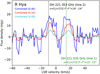 |
Fig. 19 R Hya spectra of the F′ − F″ = 13−13 and 14−14 hyperfine transitions of OH in the υ = 0, J = 27/2 rotational transition (lines 1 and 2 in Table 3) extracted from combined high and mid spatial resolution data for an aperture diameter of 0.″08, 0.″16 and 0.″40. The spectra are converted from the observed frequency to the LSR frame using the line 2 rest frequency as the “reference” frequency. The black dotted vertical line (line 2) is at the adopted new systemic velocity (see Table 1). The green dotted vertical line is displaced by ~24.3 km s−1 compared to line 2 as expected from the υ = 0, J = 27/2 Λ-doublet frequency separation; it corresponds to line 1. |
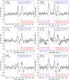 |
Fig. 20 Spectra of R Hya, S Pav and R Aql in the J = 27/2 and 29/2 rotational levels of OH extracted from the high resolution data cubes for an aperture diameter of 0/08. The three left and three right panels correspond to J = 27/2 and 29/2, respectively. In each spectrum, the two nearby emission features correspond to the two hyperfine transitions of each A-doublet (dotted blue and red vertical lines). Note weak absorption features observed in all six spectra. In the J = 29/2 spectra, the most negative velocity emission feature (closest to the F′ – F″ = 15–15 transition) is the 252.172 GHz line of water. The spectra are converted from the observed frequency to the LSR frame using the OH catalog line rest frequencies given in Table 3. Line 2 at 221353.48 MHz and line 8 at 252145.35 MHz are taken as the reference frequencies for each spectrum in the J = 27/2 and 29/2 states; they are placed at the adopted new systemic velocities (see Table 1). |
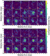 |
Fig. 21 High resolution channel maps of J = 29/2, F′ – F″= 14 – 14 and 15–15 transitions of OH in R Hya (upper and lower panels, respectively). Each map covers 200 × 200 mas and is centered on the continuum emission peak at (0,0) position (coordinates given in Table 1). Each channel velocity is in the LSR frame using the OH catalog rest frequency in Table 3. The white contours are at −3, 3 and 5σ. The line peak flux density and the typical r.m.s. noise are 9 mJy beam−1 and 1 mJy beam−1, respectively. The red contour delineates the extent at half peak intensity of the continuum emission. The line and continuum beams are shown at the bottom left of each map in white and dark-red, respectively. The HPBW is (39 × 31) mas at PA 46° and (34 × 25) mas at PA 67° for line and continuum, respectively. |
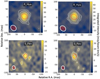 |
Fig. 22 Zeroth moment map of OH emission in the J = 29/2, F′ – F″ = 14–14 and 15–15 transitions. Left panels: F′ – F″ = 14–14 transition in R Hya and S Pav. Right panels: F′ – F″ = 15–15 transition in the same sources. Offsets in RA and Dec directions are relative to the coordinates of the peak: stellar continuum as given in Table 1. The velocity intervals in the F′ – F″ = 14–14 and 15–15 transitions are: −11.8 to −2. 6 km s−1 and −12.2 to −1.7 km s−1 in R Hya; −21. 1 to −13.8 km s−1 and −21.2 to −11.9 km s−1 in S Pav. In each map the white contours are at 3 and 5σ. The red contour delineates the extent at half peak intensity of the continuum emission. The line and continuum beams are shown at. the bottom left of each map in white and dark-red, respectively. The line HPBW in R Hya is as in Fig. 21; in S Pav the line HPBW is (25 × 20) mas at PA 11°. The continuum beam is (34 × 25) mas at PA 67° (R Hya) and (25 × 20) mas at PA −13° (S Pav). |
8.2.2 OH absorption maps and OH gas infat
The R Hya, S Pav and RAql spectra extracted from the high resolution data cubes show that there are absorption features tn addition to the two main hyperfine transitions of OH seen in emission in She J = 27/2and 29/2 levels (Fig. 20). Our images suggest that the absorption observed at velocities greater than the systemic velocity of each hyperfine transition in J = 27/2 and 29/2 is due to OH gas that is redshifted wish respect to each one of these two transition. In this scenario, the absorption seen in-between the two hyperfine transitions (Fig. 20) is interpreted as redshifted gas for the higher frequency transition of the two hyperfine transitions in each J level. (There is no apparent blueshifted OH component observed in our data for the higher frequency line of each OH Λ-doublet. This could perhaps be understood as dominant absorption by the cooled gas when it falls back to the star surface.) In the redshifted gas interpretation the OH gas falls with velocities ∼5−10 km s−1 toward the warm gas which excites each one of the two hyperfine components near the star. This is the same range as the infall velocities of H2O and CO mentioned in Sect. 5.4. OH gas infall is supported by the mom 0 maps of the absorption features showing compact OH gas centered on the star (Fig. 23), and by the ∼5−12 signal-fo-noise ratio observed at the absorption peaks toward R Aql, S Pav and R Hya (Table 8). The typical angular extent of the OH absorption above 3σ is determined as for the emission region in Sect. 8.2.1. It is smaller than the OH emission extent and on the order of 30–40 mas tn R Aql and less or comparable to the beam toward R Hya and S Pav (Table 8).
8.2.3 Current and further identification of OH sources
We have estimated typical OH scale lengths in Sects. 8.2.1 and 8.2.2, but the J = 27/2 and 29/2OH emission or absorption is often weak. In addition, and for all sources, the J = 33/2 and 35/2 rotational levels were not detected in emission or absorption at the time of our observations. In order to push further the OH detection limit and to better discern the diffuse gas, we have stacked together our data for all four hyperfine transitions with similar energy levels (i.e., J = 27/2 transitions together with 29/2, and J = 33/2 transitions with 35/2). For each group of four transitions, the visibility data were extracted for the same velocity range centered on each hyperfine transition and combined by aligning the velocities. This allows us to image four stacked hyperfine lines, reducing the noise by a factor of two, but at the expense of the identification by another approach to know which exact hyperfine transition(s) is(are) excited. If a group of four stacked transitions was detected we also stacked both component pairs separately to identify which rotational transition was detectable. Spectra were also extracted with the stacked maps to help us identify the hyperfine transitions. The F′ – F″ assignment of a rotational transition can be safely done only if the individual hyperfine transitions are visible in channel maps and/or in mom 0 maps. We have validated this approach by comparing the stacked maps with the single frequency channel maps of our strongest sources.
We conclude that there is OH emission and/or absorption in nine sources of the ATOMIUM sample in the υ = 0, J = 27/2 and/or 29/2 rotational levels including weak emission from RW Sco and IRC+10011. (In these two sources inspection of channel maps and extracted spectra suggest emission from the J = 29/2 state only.) Overall, there are slightly more detections in J = 29/2 than in 27/2 (see last column in Table 3). Four sources, R Hya, R Aql, U Her and T Mic are detected in the higher energy rotational levels υ = 0, J = 33/2 and only R Hya is observed in J = 35/2. In U Her and T Mic, OH is detected when the υ = 0, J = 33/2 and 35/2 levels are stacked together, so we cannot distinguish whether one or both rotational levels are emitting. However, since the J = 35/2 emission is very weak and observed in R Hya only, we have arbitrarily assigned the emission observed in U Her and T Mic (last column in Table 3) to the lower energy level, that is J = 33/2. We further note that the υ = 0, J = 33/2 level energy (∼8000 K) is close to the energy of the two highest H2O levels observed in this work. Four υ = 1 hyperfine transitions in the J = 31/2 and 33/2 rotational levels (with energy ∼11 080 and 12 800 K) also fall in our frequency setup but were not detected here. This nondetection is in contrast with the υ = 1, J = 21 /2 and 35/2 observations of Khouri et al. (2019) in W Hya and is discussed at the end of Sect. 9.3.
At the time of this work, high-J OH sources have been discovered with ALMA in twelve and probably thirteen AGBs or RSGs. Nine objects are listed in Tables 1 and 3, three other sources, W Hya, R Dor and IK Tau have been detected by Khouri et al. (2019), and we further report in Appendix F on the potential detection of J = 35/2 and 31/2 OH emission in omi Cet (Mira). More high-J OH transitions obtained in future ALMA observations or extracted from ALMA archival data of evolved late-type stars will contribute to our understanding of the role of OH in the formation of water and dust-forming metal oxides/hydroxides.
Peak flux density, r.m.s. noise and angular size in zeroth moment maps of OH emission and absorption.
9 A high-J OH analysis: Physical conditions
As mentioned in Sect. 8.1, no hyperfine transitions of the OH radical were ever identified in high-J levels toward evolved stars before ALMA20. Our discussion below is limited to simple estimates of the physical conditions in the high-J OH gas observed in the photospheric environment.
9.1 Line intensity ratios, brightness temperature
As a first approach to the understanding of the OH excitation conditions we compare the observed ratio of two hyperfine transitions in a given rotational level with the same ratio under LTE conditions. There are several difficulties in estimating such ratios from the ΔF = 0 line parameters. Fitting Gaussians to weak, asymmetrical line profiles is uncertain. Nevertheless, the peak line flux density is often well identified and if not, we can derive the integrated flux density across the line profile above the noise level. Our results in five stars, foe both line peck and integrated flux density ratios above 3σ, are gathered in Tabl2 9 together with the LTE line opacity ratios. All ratios are derived from spectra extracted from the high resolution data cubes for an aperture diameter of 0.″08. We have also verified that for R Hya in the J = 27/2 and 29/2 levels, the intensity ratios remain similar, within the uncertainties to those obtained with the mid resolution data. For the higher J = 33/2 and 3512 levels, when only one hyperfine transition is detected we give a lower limit based on the 3σ level outside the expected but undetected line feature. The formal uncertainty of our intensity ratios is estimated to be in the range 0.10−0.15 except, in the J = 33/2 level where it is significantly higher due to the tower S/N. The line integrated flux density ratio and the peak flux density ratio (see Integr. ratio and Peak ratio columns in Table 9, respectively) give comparable results in general. In R Hya, for example, the peak ratios are equal to 0.96 and 0.93 for J = 27/2 and 29/2. respectively, while the integrated flux density ratios are somewhat smaller but still consistent, within the uncertainties, with the LTE ratios. However, deviations from LTE are significantly above the uncertainties for R Aql and S Pav (∼1.1–1.6) in the J = 27/2 level and for VX Sgr and T Mic (∼0.7–0.8) in J = 29/2. The observed peak intensity ratios are larger than the LTE ratios for J = 33/2 and J = 35/2 observed in R Aql and R Hya These results show (hat the OH gas is not excited under full LTE conditions, and there are no strong masers obcerved in the high-J levels. Deviations from LTE remain moderate when compared with the strong J = 3/2 ground state masers observed around 1.6 GHz when they were first discovered (Wilson & Barrett 1968) and in all other subsequent observations of late-type M star.
Tabte 10 gives the OH peak surface brightness in the J = 27/2 and 29/2 rotational leve, Sp, derived from our channel maps for the extended configuration and for beam widths ranging from~25 × 23 mas (T Mic) to ~41 × 30 mas (R Hya). For simplicity, Sp is only given for the brightest of the two hyperfine transitions J = 27/2, 14–14 and J = 29/2, 15–15. The peak brightness temperature. Tb, is derived from Sp and the restoring beam. It gives an estimate of the maximum brightness temperature for OH emitting region sizes on the order of one or a few beams. Tb is a lower limit to the brightness temperature ii the region is smaller than the synihesized beam or made up of multiple clouds (or if- maser beaming narrows the measured angular size in individual channel, although masing is unlikely in OH high-J levels). Table 10 gives values of Sp and Tb in the ∼3–9 mJy beam−1 and ∼100−280 K, respectively. These values of Tb are lower than the local TK and suggest that the OH excitation conditions are close to LTE (in agreement with the intensity ratios in Table 9), and that the OH lines are optically thin.
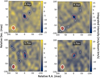 |
Fig. 23 Zeroth moment map of OH absorption in the J = 27/2, F′ – F″ = 14–14 and 13–13 transitions. Leftpanels: F′– F″ = 14–14 transition in R Aql and S Pav. Right panels: F′ – F″ = 13–13 transition in the same sources. Offsets in RA and Dec. directions are relative to the coordinates of the peak stellar− continuum as given in Tattle 1. The velocity intervals in the F′ – F″ = 14–14 and 13–13 transitions are: 55.8 to 61.2 km s−1 and 56.2 to 66.2 km s−1 in R Aql; −10.2 to −3.6 km s−1 and −9.4 to 33.5 km s−1 in S Pav The dotted white contours are at −33 and −5σ The red contour delineates the extent at half peak intensity of the continuum emission. The line and continuum beams are shown at the bottom left of each map in white and dark-red, respectively. The line HPBW is (27 × 22 mas) at PA 18° and (27 × 21) mas at PA −3° in R Aql and S Pav, respectively. The continuum beam is (24 × 22 mas at: PA −13 (R Hya) and (25 × 20) mas at PA −13° (S Pav). |
Observed integrated flux density and peak flux density ratios (Integr. ratio and Peak ratio) and LTE opacity ratio of OH hyperfine transitions in J = 27/2, 29/2, 33/2 and 35/2.
Peak surface brightness (Sp), peak brightness temperature (Tb) and uncertainty in the J = 27/2 and 29/2 rotational levels of OH.
9.2 Population diagrams and opacity estimates
An estimate of the OH rotational temperature, Trot, and column density, N(OH), can be obtained from a population diagram although this is uncertain because the detected OH transitions span a moderate range of upper energy levels. As for H2O, we have used the high resolution data, all observed within a few weeks. The S/N of the integrated OH line intensity is on the order of 6–10 in R Hya, S Pav and R Aql in the J = 27/2 and 29/2 levels and less (or undetected) in J = 33/2 and 35/2. We have plotted population diagrams for these three sources (Fig. 24) but, unfortunately, there are not enough detected OH transitions in other stars to estimate N(OH), including AH Sco and IRC+10011 for which N(H2O) is determined (Fig. 11). The partition function used to derive N(OH) is obtained from a direct summation of the energy levels in different vibrational states and from parameters based on the JPL catalog data; all components due to Λ and spin doublings and the hyperfine structure have been included As for H2O, the partition function varies mono-tonically with the temperature and N(OH) is not very sensitive to uncertainties in the values of Trot. We derive Trot ∼ 2800 and 3000 K and N ∼6.1 × 10¹⁸ and 4.8 × 1018 cm−2 in R Hya and S Pav, respectively. In R Aql, Trot is higher, ∼4000 K, and N(OH) ∼4.3 × 1018 cm−2. The main limitations in the determination of N(OH) come from the rather restricted energy range and the fact that the observed regions are assumed to have uniform properties. However, tests made with various assumed errors in the observables suggest that N(OH) can vary by at least 30%.
Using N and Trot obtained above, we get an opacity at the OH emission line center in the range τC ∼0.02−0.03 in both J = 27/2 and 29/2. (The opacity in a given J level does not vary significantly from one hyperfine transition to the other.) These opacity estimates are in rough agreement with the ratio (Tb/Trot) which suggests that the OH emitting region cannot be much smaller than the beam.
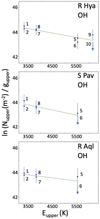 |
Fig. 24 OH population diagram for R Hya, S Pav and R Aql. The number near each data point is the line number used in Table 3 of observable OH transitions. The vertical bar in each data point includes the ±1σ formal error of the integrated flux density and a rough estimate of the filling factor uncertainty. (An arrow indicate an upper limit.) Τhe green line is the regression line across the data points (see Sect. 9.2). |
9.3 Lack of v = 1 OH emission and implications
The lack of υ = 1 OH emission from R Hya, our strongest OH source, even after the OH lines have been stacked, is surprising when compared to the relatively strong hyperfine transitions of the υ = 1, J = 21 /2 and J = 35/2 levels observed by Khouri et al. (2019) in the Mira variable W Hya around the optical phase 1.0–1.1. In R Hya, our 3σ upper limit in the υ =1, J = 31/2 and 33/2 spectra is ∼3 mJy (for an aperture diameter of 0.″08) around the optical phase 0.8, whereas the υ = 0, J = 27/2 and 29/2 emissions peak around 10–15 mJy (see Fig. 20). There is no OH υ = 1 detection toward R Aql and S Pav (upper limits around 3 to 10 mJy) observed around the optical phases 0.2 and 0.9. Changing the extracted aperture area for our spectra or considering the mid resolution data do not show any υ = 1 detection either.
We cannot exclude that the high-J OH excitation in both υ = 0 and 1 are time variable and may depend on the stellar optical phase. Our OH observations of R Hya and other targets have been acquired at essentially a single epoch and with often too low S/N to usefully address time variability issues in individual stars. However, despite the pulsation period of any one star not being well sampled, the whole set of objects observed at several epochs may be considered as covering a range of optical phases and we might have hoped to observe υ = 1 OH emission in at least one star21.
It is interesting to note that time-variable, near IR excitation of OH in the υ = 0 to υ =1 transition at 2.8 μm was invoked by Harvey et al. (1974) to explain the 18-cm OH variations observed in late-type stars. But later, Etoka & Le Squeren (2000) showed that the phase delay observed between the 18-cm OH maser peak emission and the near IR maxima suggests that dust in the outer layers contributes in the OH excitation. The pumping mechanism proposed for the ground state of OH, however, cannot explain the potential excitation of high-J OH levels in the inner gas layers of O-rich stars.
The possible role played by the 2.8μm radiation in the excitation of the high-J OH transitions observed in the inner gas layers, can be crudely appreciated from an estimate of the critical gas density, nc, for the υ = 0 to υ =1 transition. Taking 16.9 s−1 for the spontaneous emission rate (Brooke et al. 2016), and assuming that the collisional rate coefficient of OH with H2 is dominated by rotational transitions and can be represented by ∼2 × 10⁻¹⁰(TK/100)0.5 cm3 s−1 (Klos et al. 2017), we obtain nc ∼8.5 × 10¹⁰/(TK/100)0.5, that is ∼1.5−5 × 1010 cm−3 for TK in the range 300 to 3000 K. A similar density range also applies to the υ = 2 to υ = 1 transition with 23.4 s−1 spontaneous emission rate. Therefore, we expect that collisions play a significant role in the vibrational line excitation of OH within the high density regions close to the photosphere where OH is formed after the passage of shocks. We also expect that changing physical conditions resulting from stellar pulsations and shocks in regions where the high- J optically thin OH microwave lines are observed may lead to both υ = 0 and 1 OH line variability. This may perhaps explain why υ = 1 OH lines observed by Khouri et al. (2019) are not detected in this work. However, questions related to high-J OH time variability deserve dedicated sensitive mm-wave observations in the future.
10 Observed OH/H2O abundance ratio and chemical models in the inner wind
We primarily wish here to compare the OH/H2O abundance ratio derived from our estimates of the H2O and OH column densities with the same ratio predicted from chemical models. From the high resolution observation of high-lying energy levels of three AGBs (R Hya, S Pav and R Aql), all performed within a few weeks, and from the population diagram analysis described in Sects. 5.2 and 9.2, we obtain N(OH)/N(H2O) ∼(0.7−2.8) × 10−2. Assuming, as suggested from the ALMA maps, that the observed H2O and OH transitions come from similar regions in the circumstellar inner wind, we thus expect OH/H2O ∼0.7−2.8 × 10⁻², which will be compared with our recent chemical models. We first make some general and brief considerations on the chemical context in evolved stars and on the model outputs predicting H2O and OH fractional abundances for regions up to ⪝10 R⋆. The chemical equilibrium conditions of an ideal LTE atmosphere (e.g., Tsuji 1973) can explain the formation of various molecules observed in cool stars as well as their dependence on the C/O ratio (i.e., the molecular fractional abundances critically depend on the evolutionary status of the star). However, in the outer stellar atmosphere, convection and stellar pulsations imply that equilibrium conditions are rapidly changing with time or position. Predicting the chemical composition of the gas becomes complicated because of the generation and propagation of shocks, the formation of dust particles and the launch of an inner stellar wind. In such a complex environment, we know that a rich, nonequilibrium chemistry is possible and is supported by the observation of a large variety of molecular species in the IR (e.g., Tsuji et al. 1997) and in the mm/submm domains, including the unexpected presence of H2O in C-rich stars (Neufeld et al. 2011) or of HCN in O-rich stars (Lindqvist et al. 1988; Justtanont et al. 2012). Decoupling the hydrodynamics of the inner wind from the chemistry, Willacy & Cherchneff (1998) and Cherchneff (2006) have predicted the molecular abundances of several species including H2O and OH in the ∼1 −5 R⋆ region. Later, Gobrecht et al. (2016) confirmed that periodic shocks in the IK Tau environment provide efficient conditions for the synthesis of various chemical species and dust nucleation in the range ∼1−10 R⋆. Boulangier et al. (2019) further showed that a nonequilibrium chemistry leading to dust nucleation impacts the dynamics of the wind and, recently, Gobrecht et al. (2022) gave new details on dust nucleation scenarios.
The observed abundance ratio, OH/H2O ∼ (0.77−2.8) × 10−2, despite uncertainties, can be directly compared with various model predictions. In typical O-rich stars and for C/O ratios ∼0.75, Cherchneff (2006) obtained a rather flat distribution of the OH and H2O abundance s between ∼1.5−5 R⋆ from which we get OH/H2O in the range 10−3 to 2.55 × 10⁻⁵; these ratios are far from our observational estimates. To model the dust formation and the chemical atmosphere of IK Tau, Gobrecht et al. (2016) derived the molecular content between 1 and 10 R⋆ as well as the abundance variation with the stellar pulsation phase at different radii. The H2O abundance relative to the total gas density remains Hat and around 10−4 up) to 20 stellar radii. This is sligghtly smaller than the 4 to 2 × 10⁻⁴ H2O fractional abundance obtained by Cherchneff (2006) between 1 and 5 R*. It is thus useful to revisit the chemical model ot Gobrecht et al. (2016) using the more recent kinetic rates given in Gobrecht et al. (2022). Our newer calculations for radii between 1 and 10 R⋆, before the wind is fully accelerated, predici that for typical Mira-type and semi-regular variadiles the OH-H2O ratio varies by one to two orders of magnitude at different pulsation phases (0.2, 05 and 1.0 in Fig. 25). (We point out that at the present time we have no model outputs available for RSGs.) The decrease observed with the radial distance irr the OH/H2O ratio (Fig. 25) is driven by the decrease in the OH abundance while the H2O abundance remains roughly at the same level within the inner gas layers as seen in Fig. 22 of Gobrecht et al. (2022). The larger dispersion in the OH/H2O ratios of the Mira-type stars with respect to the semi-regular variables is most probably explained by the stronger shock; and lower (preshock) temperatures in the Mira-like models Our calculations suggest that in the range from 2 to 3 R⋆ the predicted OH/H2O ratios approach those derived from the ATOMIUM observations at optical phases ∼0.5−0.2. However, our current observations, lacking data at different; epochs are unable to estimate how the OH/H2O ratio varies with the optical phase and if variations mach the model predictions. In addition, we note that there might be some mirror phase shift between pulsation and optical phase (Liljegren et al. 2016.
The OH/H2O ratio is primarily controiledby (he reaction pair H2 + OH <−> H2O + H (ΔHr(0 K) = −56 kJmol−1). The forward reaction rate has an activation barrier of 1660 K whereas the endothermic reverse reaction has a much higher activation energy of 9720 K (Baulch et al. 1992). Therefore, the larger OH/H2O ratios at pulsation phase 0.2, ranging from ∼4 × 10⁻² to 2 in Mira-type variables, can be explained by comparatively higher temperatures. At these high temperatures not; only the reverse reaction is activated, but also the atomic hydrogen is abundant. In contrast, at later pulsation phases (around 1.0) low temperatures prevail and hydrogen is predominantly molecular. As a consequencv, the H2O-forming forward reaction dominates at laie puliation phases and the reverse reaction is negligible, leading to low OH/H2O ratios ∼8 × 10⁻⁶ to 7 × 10⁻⁴. In general, we note in our models a greater dependence of the OH/H2O ratio on time (or pulsation phase) than on distance from the star at a given pulsation phase.
It is interesting to mention that the excitation of high-J levels of OH in the inner gas layers could eventually be triggered by ihe photodissociation of water from the UV radiation generated in the outflow shocks of pulsating stars. This could lead to the selective formation ot high-J OH states as suggested in Tappe et al. (2008) for the young stellar object HH 211 outflow. How-ever, the shock speeds invoked in this woak, at least 40 km s−1, are higher than those observed in AGBs. Therefore, we favor the direct formation of OH from oxrygen and H2 after the passage of the circumstellar shock, although special cases are also possible; for example readers can refer to the UV photon models -from a stellar companion impccting the chemical products, for example (van de Sande & Millar 2022).
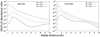 |
Fig. 25 Model predictions of the OH/H2O abundance ratio versus the radial distance at different pulsation phases of Mira-type and semi-regular variables. The spread in the abundance ratio versus the radial distance and the optical phase is discussed in Sect. 10. |
11 Concluding remarks
Ten rotational transitions in the ground and excited vibrational state of  were observed in the 213.83–269.71 GHz frequency range of the ATOMIUM Band 6 survey undertaken with the ALMA main array. Nine lines are new discoveries and the tenth, reported earlier at 268.149 GHz in two evolved stars, was observed in the 15 O-rich sources of the 27 late-type stare in our sample. High spectral resolution observations at an additional epoch were also undertaken with the ACA around 268 GHz and 254 GHz. The ten transitions, six in the ortho state and four in the para state of H2O, include six pure rotational transitions within a single excited vibrational state, two ro-vtbrational transitions between two nearby vibrational states, and two pure rotational transitions in the ground vibrational state. Together they span a range in excitation energy of between 3950 K in the ground vibrational state to 9013 K in the (υ1,υ2,υ3) = (0,0,1) state. Our observations significantly extend the number of H2O transitions that have been observed in evolved stars in the radio domain.
In parallel, the hyperfine split Λ-doubling transitions in the υ = 0, J = 27/2 and 29/2 high-lying rotational levels in the Χ2Π3/2 state of OH, as well as the υ = 0, J = 33/2 rotational level in the upper Χ2Π1/2 state have been observed in the same Band 6 spectral line survey. The next higher Λ-doubling transition, J = 35/2, was observed in one star only (R Hya)22. The range of energy levels covered by the OH lines observed here is ∼4780–5500 K and -8000–8900 K.
11.1 H2O
Some general trends have emerged from our extensive high resolution observations. The sections where our main results are presented and discussed are specified at the end of each paragraph below.
There is good agreement between the rest frequencies determined from the present observations and the frequencies measured in the laboratory. In those cases where the catalog frequencies were derived with uncertainties exceeding ∼0.5 MHz, our rest frequencies could be better than the catalog frequencies (see Sect. 3.2).
Overall the H2O emission observed with the extended configuration is compact and observed in regions extending from a few to about 12 R⋆ from the central star. Possible extensions up to ∼20–30 R⋆ were also observed at 268.149 GHz (see Sect. 4.3).
The number of stars in which an H2O line was detected is roughly two times higher for transitions that arise in lower-lying levels (∼4000–5600 K) than in the higher-lying levels (∼8000–9000 K). There does not appear to be any correlation between the number of detected transitions and the physical parameters of the source such as the mass-loss rate (see Sect. 4.1).
The three most intense and widespread transitions in H2O are the ortho line at 268.149 GHz in the (0,2,0) vibra-tional state which was observed in 15 stars, the para lines at 262.898 GHz in the (0,1,0) state which was observed in 12 stars, and 259.952 GHz in the ground vibrational state which was observed in ten stars. A line was also observed in the (0,3,0) vibrational state in eight stars, in the (0,0,1) state in nine stars, and the ro-vibrational transition
 was observed in eight stars (see Sect. 3.2).
Both emission and absorption are observed in our maps and spectra of H2O (and the same applies in OH). In a few stars, zeroth moment maps reveal absorbing regions as small as ≲20–40 mas that are closely associated with the central star and are redshifted by a few km s−1 with respect to the gas layers seen in emission. Infall velocities of 5–10 km s−1 that were estimated from our H2O observations and from υ =1, CO observations are close to model predictions from Nowotny et al. (2010, see Sects. 4.4 and 5.4).
A Gaussian analysis of the most compact emission regions in two prominent H2O sources in the survey has revealed an organized (R Hya) and a complex (U Her) position-velocity emission structure (see Sect. 4.5).
High velocity wings of the 268.149 GHz line emission with respect to υ = 0, CO emission were observed in several stars. The most probable explanations include local turbulence or kinematic perturbations by a companion (see Sect. 5.4).
We have derived beam-averaged column densities from our H2O population diagrams in AH Sco, R Aql, R Hya, S Pav, and IRC+10011. They lie in the range ∼(0.6−5) × 1020 cm−2 (see Sect. 5.2).
The 268.149 GHz transition which is observed in all but the two S-type stars may be excited under quasi-LTE conditions or is masing in at least three stars (U Her, AH Sco, and IRC+10011) with brightness temperatures in the range 104−107 K. Time variability and line profile narrowing have also been observed in our data. Among the two other strongest H2O lines in the ATOM-IUM survey, signs of maser emission have also been observed at 262.898 GHz with time variable emission in some velocity channels of IRC+10011 (see Sects. 5.1, 6.1 to 6.4).
Based on H2O radiative transfer models in Gray et al. (2016), density, kinetic temperature, and dust temperature conditions leading to maser emission have been revisited. The 268.149 GHz line in the (0,2,0) vibrational state has a strong radiative pumping component similar to several other ortho and para H2O line pairs in the (0,1,0) state (see Sect. 7).
11.2 OH
Refined OH Λ-doubling frequencies have been made possible from ALMA high-J OH observations. Nine high-J OH sources of the ATOMIUM sample have been discovered and their characteristics are summarized below.
Based on our OH observations and those published in Khouri et al. (2019), new, accurate Λ-doubling frequencies for high-J level transitions have been derived (see Sect. 3.4 and Appendix A).
The main sources of OH observed in this work in the Λ-doubling transitions of the Χ2Π3/2, J = 27/2 and 29/2 states are: the SR and Mira variables R Hya, R Aql, S Pav, U Her, and T Mic; and the RSGs AH Sco and VX Sgr. The lines are weak, with peak intensities that range between 3 and 10 mJybeam−1. We did not observe strong deviations from the quasi-LTE line excitation conditions in our data (see Sects. 8.2.1 and 9.1).
Very weak OH emission was also identified by stacking the spectra at the expected frequencies of the hyperfine split components in RW Sco and IRC+10011. We also extracted weak OH emission in Mira from the ALMA archive (see Sect. 8.2.3 and Appendix F).
Most of the OH emission is centered on the stellar photosphere and there is weak diffuse OH emission that extends well beyond the stellar continuum sources. In SR and Mira variables, the estimated angular size of the OH emission is ∼5–8 R⋆, in general, with possible extensions up to ∼10 R⋆ from the photosphere (see Sect. 8.2.1).
In addition to the two main OH emission profiles in each Λ doublet, our spectra and maps strongly suggest that OH absorption is also present with features that are redshifted by −5 to −10 km s−1. This is comparable to the velocity of the infall layers observed in H2O and in the υ = 1, CO line. The absorption is barely resolved and typical angular scales are ≲30–40 mas in R Aql, R Hya, and S Pav (see Sect. 8.2.2).
We have observed the Λ-doubling transitions in the J = 33/2 rotational level of the Χ2Π1/2 state in four sources (R Hya, R Aql, U Her, and T Mic), but the next higher rotational level in the Χ2Π1/2 state (J = 35/2) was only detected in R Hya. These lines are very weak and observed by stacking the spectra at the frequencies in the J = 33/2 and J = 35/2 levels23 (see Sect. 8.2.3).
The OH emission from the two RSGs AH Sco and VX Sgr exhibits complex emitting regions. In both stars weak OH emission extends beyond the central object up to ∼15 R⋆, which is larger than the typical OH sizes observed in the AGBs. In both RSGs the mom 0 maps reveal asymmetric extensions in the J = 29/2 state (see Sect. 8.2.1).
Estimates of the column density of OH in the ground vibra-tional state were derived from rotational temperature diagrams that include the two successive Λ-doubling transitions in the X2Π3/2 state, and the lower of the two Λ transitions in the X2Π1/2 state of S Pav and R Aql, and both Λ-doublet transitions in the X2Π1/2 state in R Hya. We obtained 4.3,4.8, and 6.1 × 1018 cm−2 in R Aql, S Pav, and R Hya, respectively (see Sect. 9.2).
11.3 Chemical abundances and prospective remarks
From our determinations of the H2O and OH column densities, and on the assumption that both species are excited in similar regions, we derived – from R Hya, S Pav, and R Aql – an OH/H2O ratio of ∼0.7−2.8 × 10⁻², thereby establishing a benchmark for predictions of the chemical abundances in the inner wind of oxygen-rich AGBs by the chemical kinetic codes. One of the caveats in our determination of the OH/H2O ratio is that a more stringent test of the accuracy of the chemical kinetic predictions awaits measurements of the OH/H2O ratio as a function of the optical phase of the pulsating SR and Mira variables. Prior theoretical estimates of the OH/H2O ratio ranged between about 10−3 to 10−5 (e.g., Cherchneff 2006). In our work we find, with updated chemical kinetic rates (Gobrecht et al. 2022), that the chemistry in the inner wind of a typical SR or Mira variable predicts a strong dependence of the OH/H2O ratio on the pulsation phase of the star. Furthermore, OH/H2O ratio variations by one to two orders of magnitude or even more around a given pulsation phase are possible in the 1–10 R⋆ range.
Despite the whole set of observed stars covering a range of optical phases, we have not, with the ATOMIUM data, systematically monitored the H2O and OH line emission at different epochs in the pulsation cycle, and hence any evidence for time variability of the OH/H2O ratio cannot be accurately examined. However, time variability is present in the H2O data. It is well documented in U Her, observed in two epochs with the mid-configuration, and in a few other stars observed with the extended configuration and the ACA.
We conclude with two remarks: (1) an in-depth test of the chemical kinetic predictions awaits dedicated monitoring of the H2O and OH emission in R Hya, S Pav, and R Aql, and possibly other SR and Mira variables. (2) An in-depth development of H2O line excitation models awaits newer collision rates and needs to incorporate higher vibrational states, hopefully up to the (0,3,0), (1,1,0) and (0,1,1) states, together with line overlap effects between para and ortho water.
Acknowledgements
The authors gratefully thank the referee for his careful reading of the manuscript and his most constructive comments. This paper makes use of the following ALMA Main Array and ACA data: ADS/JAO.ALMA#2018.1.00659.L (ATOMIUM: ALMA tracing the origins of molecules in dust forming oxygen-rich M-type stars); #2019.2.00234.S (The remarkable 268 GHz line of water: a new tracer of the inner wind of evolved stars?); #2017.1.00393.S and #2018.1.00749.S (Bands 6 and 7 data used for the OH spectra in Mira, Appendix F). The standard ALMA pipeline products are available in the ALMA Science Archive (ASA). The enhanced products prepared by the ATOMIUM consortium, once ingested, will become available during or soon after publication of this paper. ALMA is a partnership of ESO (representing its member states), NSF (USA) and NINS (Japan), together with NRC (Canada), NSC and ASIAA (Taiwan), and KASI (Republic of Korea), in cooperation with the Republic of Chile. The Joint ALMA Observatory is operated by ESO, AUI/NRAO and NAOJ. A.B. and F.H. acknowledge financial support from ‘Programme National de Physique Stellaire’ (PNPS) of CNRS/INSU, France and ANR PEPPER. T.D. acknowledges support from the Research Foundation Flanders (FWO) through grant 12N9920N and is supported in part by the Australian Research Council through a Discovery Early Career Researcher Award (DE230100183). K.T.W. acknowledges support from the European Research Council (ERC) under the European Union’s Horizon 2020 research and innovation programme (Grant agreement no. 883867, project EXWINGS). D.G. was funded by the grant “The Origin and Fate of Dust in our Universe” from the Knut and Alice Wallenberg Foundation. T.J.M. thanks the Leverhulme Trust for the award of an Emeritus fellowship. Calculations in Sect. 7 used the DiRAC Data Intensive service at Leicester, operated by the University of Leicester IT Services, which forms part of the STFC DiRAC HPC Facility (www.dirac.ac.uk). The equipment was funded by BEIS capital funding via STFC capital grants ST/K000373/1 and ST/R002363/1 and STFC DiRAC Operations grant ST/R001014/1. DiRAC is part of the National e-Infrastructure. S.H.J.W. acknowledges support from the Research Foundation Flanders (FWO) through grant 1285221N. M.M. acknowledges funding from the Programme Paris Region fellowship supported by the Région Île-de-France. This project has received funding under the Framework Program for Research and Innovation “Horizon 2020” under the Marie Sklodowska-Curie grant agreement no. 945298.
Appendix A OH Λ-doubling transitions in the υ = 0 and 1 states
We have mentioned in Sect. 3.4 the short-coming of the JPL catalog to calculate Λ-doubling transitions for high rotational quantum numbers. Explanations are given in this Appendix. The Λ-doubling transitions connect transitions with the same N and J in Hund's case (b) or the same Ω and J in Hund’s case (a) and their spacing is dominated by the Λ-doubling parameters p and q. The 2Π3/2 υ = 0 fundamental transitions near 1.7 GHz were determined with a few Hertz accuracy by Hudson et al. (2006) and Lev et al. (2006). Their intensities decrease rapidly at room temperature and at modest quantum numbers. The highest rotational transitions in υ = 0 from laboratory measurements are J = 19/2 (2Π3/2) and 15/2 (2Π1/2) near 66 and 71 GHz, respectively (Kolbe et al. 1981; Drouin 2013). In υ = 1 the quantum numbers are limited to J = 13/2 for both 2Π3/2 and 2Π1/2 near 18 and 67 GHz, respectively (Andresen et al. 2000) and there are even more limitations for υ = 2. Our knowledge on the Λ-doubling transitions with higher rotational quantum numbers comes, for example, from pure rotational transitions in the far-infrared region with ∼1.2–3 MHz accuracy for the best lines (Martin-Drumel et al. 2012). In addition, these transitions depend predominantly on the rotational spacing between the upper or the lower Λ-component of two adjacent J levels and sample only the differences between the Λ-components which are only a very small fraction of the respective transition frequencies. We conclude that it is not surprising that observations suffer from deviations up to a few MHz between the calculated and observed Λ-doubling transitions with high quantum numbers and increasing vibrational states.
We have also mentioned in Sect. 3.4 that the ALMA OH line observations can be used to improve the calculation of the OH Λ-doubling transitions. We give details below.
Drouin (2013) had carried out a Dunham fit pertaining to a plethora of laboratory data. A fair fraction of the data is associated with five minor isotopic species containing 17O, 18O, or D, but this is only of minor importance for the present study. The Λ-doubling is expressed with parameters pij and qij, where p00 and q00 are the equilibrium parameters, and i and j indicate the degree of vibrational and rotational corrections to these parameters, respectively. Drouin (2013) employed 21 Λ-doubling parameters for OH itself plus five parameters to accomodate the breakdown of the Born-Oppenheimer approximation through the isotopic substitutions. (We mention specifically that the parameters used for OH without vibrational corrections were p00 to p03 and q00 to q05.) The data set from Drouin (2013) is available in the JPL catalog archive24. Two poorly determined parameters (out of 97) were omitted. We added the transition frequencies from our present study and from Khouri et al. (2019), summarized in Table 4, to the line list. We then carried out the line fit using Pickett's SPFIT program (Pickett 1991), as done earlier (Drouin 2013). Almost all changes in the values of the spectroscopic parameters were well within the 1σ uncertainties. By far the largest relative changes occurred for p02 and q02, which decreased in magnitudes by about five times the respective uncertainty; p03 and q03 decreased in magnitudes by about three times the respective uncertainty. In addition, the improvement in the parameter uncertainties was small in almost all instances; by far the largest improvement occurred for q02, where the new uncertainty was almost one third smaller. Nevertheless, as can be seen in Table 4, the changes were large enough to reproduce the Λ-doubling transitions from radio astronomy observations within uncertainties on average.
The Λ-doubling transitions derived for rotational J level energies up to ∼10000 cm−1 (or ∼14500 K) for υ = 0 and 1 are presented in four tables of this Appendix (see also end of Sect. 3.4). The reliability of our calculations is very difficult to assess; the transition frequencies with calculated uncertainties larger than 0.5 MHz should be viewed with caution. Further calculations of the OH rotational spectra in υ = 0 to 2 are available in the CDMS catalog25.
Quantum numbersa, transition frequency (Frequency), uncertainty (Unc.), lower state energy (Elow) and A value of OH Λ-doubling transitions in the υ = 0, 2Π3/2 state from our present fit.
Quantum numbersa, transition frequency (Frequency), uncertainty (Unc.), lower state energy (Elow) and A value of OH Λ-doubling transitions in the υ = 0, 2Π1/2 state from our present fit.
Quantum numbersa, transition frequency (Frequency), uncertainty (Unc.), lower state energy (Elow) and A value of OH Λ-doubling transitions in the υ = 1, 2Π3/2 state from our present fit.
Quantum numbersa, transition frequency (Frequency), uncertainty (Unc.), lower state energy (Elow) and A value of OH Λ-doubling transitions in the υ = 1, 2Π1/2 state from our present fit.
Appendix B Water line spectra
We have gathered here all spectra extracted from our extended configuration data cubes for the H2O lines 1, 5, 6, 7, 8, 10, 12, 13 and 14 listed in Table 2. For lines 12 and 14 we have also added the mid configuration spectra. The circular extraction aperture selected for each line can vary from one spectral transition to another in each source. It has been chosen so that all the emission visible in the channel maps is included in the spectra but is not too large to degrade the S/N. For some very weak detections, we used 0.″08 by default for the extended configuration spectra.
The very weak line 4 at 236.805 GHz identified in R Hya, and perhaps in S Pav, is presented for the combined extended and mid arrays in Fig. C.1.
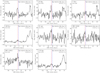 |
Fig. B.1 Spectra of line 1 at 222.014 GHz (Table 2) extracted from the extended configuration array. The extraction diameter (in arc sec) is given in parentheses below the source name in the upper left corner of each spectrum. The observed frequency is converted to the LSR frame using the catalog line rest frequency given in Table 2. The blue vertical line indicates the adopted new LSR systemic velocity (see Table 1). The red vertical line shows the LSR velocity for the slightly different frequency determined in this work (see Table 2). |
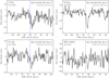 |
Fig. B.2 Spectra of line 5 at 244330 GHz (Table 2) extracted from the extended configuration array. The extraction diameter (in arc sec) is given in parentheses below the source name in the upper left corner of each spectrum. The observed frequency is converted to the LSR frame using the catalog line rest frequency given in Table 2. The blue vertical line indicates the adopted new LSR systemic velocity (see Table 1) |
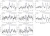 |
Fig. B.3 Spectra of line 6 at 252.172 GHz (Table 2) extracted from the extended configuration array. The rest of the figure caption is as in Fig. B.2. |
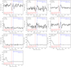 |
Fig. B.4 Spectra of lines 7 and 8 at 254.040 and 254.053 GHz (Table 2) extracted from the extended configuration array. The extraction diameter (in arc sec) is given in parentheses below the source name in the upper left corner of each spectrum. The blue and red vertical lines (lines 7 and 8) indicate the adopted new LSR systemic velocity (see Table 1) using the catalog rest frequencies (Table 2). |
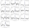 |
Fig. B.5 Spectra of line 10 at 259.952 GHz (Table 2) extracted from the extended configuration array. The rest of the figure caption is as in Fig. B.2.. |
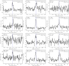 |
Fig. B.6 Spectra of line 12 at 262.898 GHz (Table 2) extracted from the extended configuration array. The rest of the figure caption is as in Fig. B.2. |
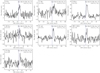 |
Fig. B.7 Spectra of line 13 at 266.574 GHz (Table 2) extracted from the extended configuration array. The rest of the figure caption is as in Fig. B.2. |
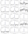 |
Fig. B.8 Spectra of line 14 at 268.149 GHz (Table 2) extracted from the extended configuration array. The rest of the figure caption is as in Fig. B.2. |
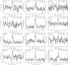 |
Fig. B.9 Spectra of line 12 at 262.898 GHz (Table 2) extracted from the mid configuration array. The rest of the figure caption is as in Fig. B.2. |
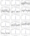 |
Fig. B.10 Spectra of line 14 at 268.149 GHz (Table 2) extracted from the mid configuration array. The rest of the figure caption is as in Fig. B.2. |
Appendix C 236.805 GHz H2O line, 254.17–254.32 GHz line emission region
Fig. C.1, upper panel, shows the water emission observed in R Hya around 236.805 GHz from the highest energy levels identified in this work (line 4 in Table 2) for different extraction diameters of the combined high and mid arrays. The spectra peak at 3.7 ± 1.5 mJy for an aperture diameter of 0.″16; the uncertainty is at the 2σ level. Peak emission around 10 mJy is also visible with the extended array alone in the same frequency range and for an aperture diameter of 0.″16. There is also an uncertain detection of the 236.805 GHz transition toward S Pav (Fig. C.1, lower panel). The spectrum is rather noisy but we observe a peak flux density of ~10 mJy with the combined array for an aperture diameter of 0.″16. Detection is less convincing around 236.805 GHz with the extended array alone.
Fig. C.2 presents the emission line profile toward two super-giants, AH Sco and VX Sgr, in the 254.17 to 254.32 GHz frequency range. There are two major features in this range, one near 254.217 GHz for the υ = 0, J = 6 − 5 transition of 30SiO, and another one around 254.28 GHz corresponding to the υ = 0,  transition of SO2, or to a blend of the latter transition with S02, υ = 0,
  . The vertical line at 254.235 GHz marks the (0,1,1) 73,4 – (1,1,0)65,1 transition of para H2O as predicted in Furtenbacher et al. (2020) (line 9 in Table 2). The weak feature observed near 254.235 GHz for the high resolution data and an aperture diameter of 0.″2 falls within ~3 MHz of the predicted water line 9 in both sources. However, the detection of line 9 is uncertain because the apparent H2O emission could just be part of the complex emission and absorption features in the blueshifted wing of the υ = 0, 30SiO line profile. We note that the 30SiO blueshifted line wing is rather steep and that the dip observed near 254.233 GHz in the line profile is visible in the extended configuration data when the diameter of the extraction aperture is ≲0.″12. This dip could thus be interpreted as the absorption signature of 30SiO material at large distances along the line of sight to the central star. Such features have been seen in the ALMA data of other evolved stars (e.g., Takigawa et al. 2021; Decin et al. 2018; Hoai et al. 2021), especially when the beam size is small compared to the angular size of the stellar disk. In addition, the radiative transfer models of Schoenberg (1988) show that a distinct blueshifted emission feature may arise from an optically thick line with extended scattering zones and, depending on the adopted turbulence, an enhanced blue line wing may also be reproduced in the CO line models (e.g., De Beck et al. 2012). Hence, our line profile in the 254.18–254.25 GHz range could just be pure 30SiO emission that is extended and optically thick. However, since both AH Sco and VX Sgr have similar terminal expansion velocities of ∼34–35 km s−1 (Gottlieb et al. 2022), it is not possible to exclude that the 254.235 GHz feature is due to water by examining these two spectra alone. We note that this feature was not observed in any AGBs of the ATOMIUM sample. Finally, we also note that the unidentified signal observed in R Hya and R Aql at 254.244 MHz (Wallström et al., in preparation) lies at about 9 MHz from the 254.235 GHz H2O (line 9); this could perhaps be due to the infall of water toward the central star.
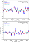 |
Fig. C.1 Spectrum of the (0,0,1) 143,12–134,9 transition of para H2O in R Hya (upper panel). Following the IPL catalog, we assume a rest frequency of 236.8054 GHz (line 4 in Table 2). The line profiles are extracted from the combined high and mid resolution data cubes for circular apertures with 0.″708, 0.″12 and 0.″16 diameters. The vertical dashed line marks the water line frequency shifted by the systemic velocity of the star |

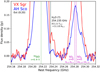 |
Fig. C.2 Emission line profiles toward AH Sco (blue) and VX Sgr (red) in the vicinity of the υ = 0, J = 6–5 transition of 30SiO (at 254.217 GHz) and of the (0,1,1) 73,4–(l, 1,0) 65,1 transition of para water near 254.235 GHz (line 9, Table 2). The spectra are extracted from the high resolution data for a circular aperture of 0.″2 diameter and plotted in the rest frequency frame. The dotted black vertical line is the expected water frequency according to Furtenbacher et al. (2020) (see Table 2). Identification of the water transition at 254.235 GHz is uncertain (see discussion in Appendix C). |
Appendix D Water channel maps and zeroth moment maps
A few channel maps obtained for the extended configuration are shown and discussed in Sect. 4.3. Additional channel maps are presented here at: 268.149 GHz (line 14) in S Pav (Fig. D.1), IRC+10011 (Fig. D.2) and the two RSGs, VX Sgr and AH Sco (Figs. D.3 and D.4); 262.898 GHz (line 12) in R Hya and U Her (Fig. D.5), S Pav and IRC+10011 (Fig. D.6) and, VX Sgr and AH Sco (Fig. D.7); 259.952 GHz (line 10) in R Hya and S Pav (Fig. D.8) and, in IRC+10011 and VX Sgr (Fig. D.9); 222.014 GHz (line 1) in R Hya and S Pav (Fig D.10), IRC+10011 and VXSgr (Fig. D.11) and, R Aql and AH Sco (Fig. D.12).
Additional mom 0 maps are also gathered in this Appendix at 222.014 GHz in R Hya, IRC+10011, VX Sgr and S Pav (Fig. D.13), and at 254.053 GHz in S Pav and R Hya (Fig. D.14).
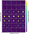 |
Fig. D.1 High resolution channel map of S Pav in the (0,2,0) 65,2−74,3 rotational transition of water at 268.149 GHz. Caption as in Fig. 6 except for the velocity range and the line peak flux density, 75 mJy/beam; the typical r.m.s. is 1 mJy/beam. The HPBW is (23×18) mas at PA 4° and (25×20) mas at PA –13° for the line and continuum, respectively. |
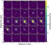 |
Fig. D.2 High resolution channel map of IRC+10011 in the (0,2,0) 65,2−74,3 rotational transition of water at 268.149 GHz. Caption as in Fig. 6 except for the velocity range and the line peak flux density, 1178 mJy/beam; the typical r.m.s. is 2 mJy/beam. The HPBW is (24×19) mas at PA 26° and (27×19) mas at PA 31° for the line and continuum, respectively. |
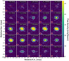 |
Fig. D.3 High resolution channel map of VX Sgr in the (0,2,0) 65,2–74,3 rotational transition of water at 268.149 GHz. Caption as in Fig. 6 except for the velocity range and the line peak flux density, 263 mJy/beam; the typical r.m.s. is 2 mJy/beam. The HPBW is (33×21) mas at PA 89° and (28×20) mas at PA 89° for the line and continuum, respectively. |
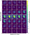 |
Fig. D.4 High resolution channel map of AH Sco in the (0,2,0) 65,2–74,3 rotational transition of water at 268.149 GHz. Caption as in Fig. 6 except for the velocity range and the line peak flux density, 60344 mJy/beam; the typical r.m.s. is 1 mJy/beam. The HPBW is (40×23) mas at PA 38° and (23×23) mas at PA 70° for the line and continuum, respectively. |
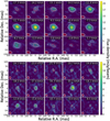 |
Fig. D.5 High resolution channel maps of R Hya and U Her in the (0,1,0) 77,1–86,2 rotational transition of water (line 12) at 262.898 GHz (upper and lower panels). Caption as in Fig. 6 except for the line frequency, velocity range and the line peak flux density, 20.9 mJy/beam (R Hya) and 16.7 mJy/beam (U Her); the typical r.m.s. is 1 mJy/beam in both stars. The line HPBW is (47×27) mas at PA 73° (R Hya) and (28×20) mas at PA 20° (U Her). The continuum HPBW is (34χ25) mas at PA 67° (R Hya) and (24×18) mas at PA 8° (U Her). |
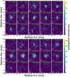 |
Fig. D.6 High resolution channel map of S Pav and IRC+10011 in the (0,1,0) 77,1–86,2 rotational transition of water (line 12) at 262.898 GHz (upper and lower panels). Caption as in Fig. 6 except for the line frequency, velocity range and the line peak flux density, 12.8 mJy/beam (S Pav) and 31.5 mJy/beam (IRC+10011); the typical r.m.s. is 1 and 2 mJybeam−1, respectively. The line HPBW is (24×18) mas at PA −20° (S Pav) and (26×20) mas at PA 22° (IRC+10011). The continuum HPBW is (25×20) mas at PA −13° ( S Pav) and (27×19) mas at PA 31° (IRC+10011). |
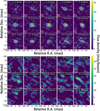 |
Fig. D.7 High resolution channel map of VX Sgr and AH Sco in the (0,1,0) 77,1–86,2 rotational transition of water (line 12) at 262.898 GHz (upper and lower panels). Caption as in Fig. 6 except for the line frequency, velocity range and the line peak flux density, 26 mJy/beam (VX Sgr) and 33.5 mJy/beam (AH Sco); the typical r.m.s. is 2 and 6.5 mJy/beam, respectively. The line HPBW is (30×22) mas at PA 80° (VX Sgr) and (45×36) mas at PA 59° (AH Sco). The continuum HPBW is (28×20) mas at PA 89° ( VX Sgr) and (23×23) mas at PA 70° (AH Sco). |
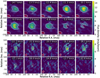 |
Fig. D.8 High resolution channel maps of relatively low energy (3954 K or 2748 cm−1) (0,0,0) 136,8−143,11 transition of water at 259.952 GHz in R Hya and S Pav (upper and lower panels). Caption as in Fig. 6 except for the velocity range and the line peak flux density, 15 and 9 mJy/beam in R Hya and S Pav, respectively; the typical r.m.s. noise is 1 mJy/beam for both stars. The HPBW is (48×28) mas at PA 72° and (34×25) mas at PA 67° for the line and continuum in R Hya, respectively, and (24×19 mas) at PA −19° (line) and (25×20) mas at PA −13° (continuum) in S Pav. |
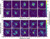 |
Fig. D.9 High resolution channel maps of water at 259.952 GHz in IRC+10011 and VX Sgr (upper and lower panels). Caption as in Fig. 6 except for the velocity range and the line peak; flux density, 26.5 and 12.2 mJy/beam in IRC+10011 and VX Sgr, respectively; the typical r.m.s. noise is 1.7 mJy/beam (IRC+10011) and 1.5 mJy/beam (VX Sgr). The HPBW is (26×19) mas at PA 24° and (27×19) mas at PA 31° for the line and continuum in IRC+10011, respectively, and (30×22) mas at PA 79° (line) and (28×20) mas at PA = 89° (continuum) in VX Sgr. |
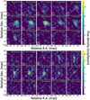 |
Fig. D.10 High resolution channel maps of high energy (8331 K) (0,3,0) 83,6–74,3 transition of H2O at 222.014 GHz in R Hya and S Pav (upper and lower panels). Caption as in Fig. 6 except for the velocity range and the line peak flux density, 9.3 and 6.5 mJy/beam in R Hya and S Pav, respectively; the typical r.m.s. noise is ~1 mJy/beam in both stars. The LSR velocity in each panel is determined from our own rest frequency, 222017.31 MHz, whose uncertainty is low compared to that in W2020 (see Table 2). The HPBW is (41×30) mas at PA = 45° and (34×25) mas at PA = 67° for the line and continuum in R Hya, respectively, and (27×21) mas at PA −3° (line) and (25×20) mas at PA −13° (continuum) in S Pav. |
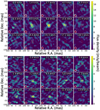 |
Fig. D.11 High resolution channel maps of water at 222.014 GHz in IRC+10011 and VX Sgr (upper and lower panels). Caption as in Fig. D.10 except for the velocity range and the line peak flux density, 17.1 and 6.4 mJy/beam in IRC+10011 and VX Sgr, respectively; the typical r.m.s. noise is 3 mJy/beam (IRC+10011) and 1.5 mJy/beam (VX Sgr). The HPBW is (30×24) mas at PA 30° and (27×19) mas at PA = 31° for the line and continuum in IRC+10011, respectively, and (31×22) mas at PA −84° (line) and (28×20) mas at PA 89° (continuum) in VX Sgr. |
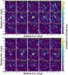 |
Fig. D.12 High resolution channel maps of water at 222.014 GHz in R Aql and AH Sco (upper and lower panels). Caption as in Fig. D.10 except for the velocity range and the line peak flux density, 6.5 and 6.8 mJy/beam in R Aql and AH Sco, respectively; the typical r.m.s. noise is 1 mJy/beam (R Aql) and 0.6 mJy/beam (AH Sco). The HPBW is (27×22) mas at PA 18° and (24×22) mas at PA = 13° for the line and continuum in R Aql, and (27×23) mas at PA 86° (line) and (23×23) mas at PA 70° (continuum) in AH Sco. |
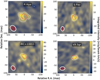 |
Fig. D.13 Zeroth moment emission maps of the (0,3,0) 83,6–74,3 transition of ortho H2O at 222.014 GHz toward R Hya, IRC+10011, VX Sgr and S Pav for the extended array configuration. The map field of view is 100×100 mas for all sources. The white contours are for 3 and 5σ emission. The red contour at the map center delineate the extent: at half peak intensity of the continuum emission. The noise tevel is 77.4, 16).0, 7.8 and 4.5 mJy/beam.km/s for R Hya, IRC+10011, VX Sgr and S Pav, respectively. The line HPBW (white ellipse) is, (41×30) mas at PA 45°, (30×24) mas at PA 30°, (31×22)) mas at PA −84° and (27×21) mai; at. PA −3° in R Hya, IRC+12011, VX Sgr and S Pav, respectively. The associated continuum HPBW (darK-red ellipse) is (34×25) mas at PA 67°, (27×19) mas at PA 31°, (28×20) mas at PA 89° and (25×20) mas at PA −13°. (Maps are integrated over −10.8 to −5.2, 14 to 15.9, −0.7 to 13.8 and −26.0 to −14.1 km s−1 for R Hya, IRC+10011, VX Sgr and S Pav, respectively.) |
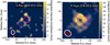 |
Fig. D.14 Comparison of the mom 0 absorption and emission of water at 254.053 GHz (line 8 in Table 2). Left panel: Absorption in S Pav is delimited by the dotted -5σ contour while the ring-like emission is shown in yellow. The noise level is 3 mJy/beam km s−1. Right panel: As for left panel but in R Hya. The noise level is 2.5 mJy/beam km s−1 In both panels the red contour at the map center delineates the extent at half peak intensity of the continuum emission. The HPBW is (24×19) mas at PA 6° and (25×20) mas at PA −13°) for the line (white ellipse) and continuum (dark-red ellipse) in S Pav, and (39×30) mas at PA 49° (line) and (34×25) mas at PA 67° (continuum) in R Hya. (The velocity intervals are: −2.6 to 6.5 km s−1 and −9.3 to −3.9 km s−1 for S Pav absorption and emission; −9.2 to −2.6 km s−1 and −19.1 to −10.5 km s−1 for R Hya absorption and emission.) |
Appendix E OH channel maps and zeroth moment maps
Additional OH channel maps obtained from the extended resolution data cubes are presented here for the J = 27/2 rotational level (Figs. E.1 and E.2 in R Hya and R Aql) and the 229/2 level (Fig. E.3 in S Pav).
Fig. E.4 shows the J = 29/2 zeroth moment maps for R Aql and VX Sgr and, zeroth moment maps in the same J = 29/2 rotational level are presented in the main text for R Hya and S Pav (Fig.22). OH zeroth moment maps in the J = 27/2 level are shown in Fig. E.5 for R Hya, S Pav, R Aql and VX Sgr.
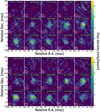 |
Fig. E.1 High resolution channel map of J = 27/2, F' – F" = 13 – 13 and 14–14 transitions of OH in R Hya (upper and lower panels, respectively). Figure caption as in Fig. 21 except for the velocity range. The line peak flux density and the r.m.s. noise level are identical to those in Fig. 21. The HPBW is (41 ×30) mas at PA 45° and (34×25) mas at PA 67° for line and continuum, respectively. |
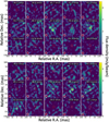 |
Fig. E.2 High resolution channel map of J = 27/2, F' – F" = 13 – 13 and 14–14 transitions of OH in R Aql (upper and lower panels, respectively). Figure caption as in Fig. 21 except for the beam widths and the velocity range. The line peak flux density and r.m.s. noise levels are ~5 and 1 mJy/beam, respectively. The line and continuum HPBWs are (27×22) mas at PA 18° and (24×22) mas at PA −13°, respectively. |
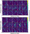 |
Fig. E.3 High resolution channel map of J = 29/2, F' – F'' = 14 – 14 and 15–15 transitions of OH in SPav (upper and lower panels, respectively). Fig. caption as in Fig. 21 except for the velocity range. The line peak flux density and r.m.s. noise level are ~6 and 1 mJy/beam, respectively. The line and continuum HPBWs are (25×20) mas at PA = 11° and (25×20) mas at PA −13°, respectively. |
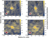 |
Fig. E.4 Zeroth moment maps of OH emission in the J = 29/2, F' – F'' = 14 – 14 (left panels) and 15 – 15 (right panels) transitions in R Aql and VX Sgr as marked. Figure caption as in Fig. 22 except for the velocity intervals in the F' – F'' = 14 – 14 and 15–15 transitions which are: 46.8 to 53.8 km s−1 and 46.4 to 53.4 km s−1 in R Aql; 3.0 to 15.8 km s−1 and 6.1 to 17.8 km s−1 in VX Sgr. The line HPBWs are (29×20) mas at PA −43° and (35×23) mas at PA −89° in R Aql and VX Sgr, respectively. The continumm HPBWs are (24×22) mas at PA −13° (R Aql) and (28×20) mas at PA 89° (VX Sgr). |
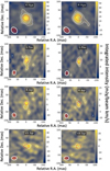 |
Fig. E.5 Zeroth moment maps of OH emission in the J = 27/2, F' – F'' = 13 – 13 (left panels) and 14 – 14 (right panels) transitions in R Hya, S Pav, R Aql and VX Sgr as marked. Figure caption as in Fig. 22 except for the velocity intervals. The velocity intervals irr the F' – F" = 13 – 13 and 14–14 transitions are: −10.7 to −4.1 km s−1 and −11.5 to −2.2 km s−1 in R Hya; −21.0 to −10.4 km s−1 and −21.8 to −12.5 km s−1 in S Pav; 43.3 to 51.3 km s;−1 and 46.6 to 51.7 km s−1 in R Aql; 2.9 to 21.5 km s−1 and 7.5 to 16.8 km s−1 in VX Sgr. The line HPBW is (41×30) mas, (27×21) mas, (27×22) mas and (31×22) mas at PA 45°, −3°, 10° and −84° in R Aql, S Pav, R Aql and VX Sgr, respectively. The continuum HPBWs are: (34×25) mas at PA 67° (R Hya), (25×20) mas at PA 13° (S Pav), (24×22) mas at PA −13° (R Aql) and (28×20) mas at PA 89° (VX Sgr). |
Appendix F Bands 6 and 7 OH lines toward omi Cet (Mira)
Using the ALMA archive, we report here on the detection of high-J hyperfine transitions of OH in the atmosphere of omi Cet (Mira). In the Band 6 data acquired with 20 mas resolution (project 2017.1.00393.S) we have identified a weak feature (S/N ∼2.5–3) near 265.735 GHz (Fig. F.1) coinciding, within the frequency uncertainties, with the υ = 0, J = 35/2, F' – F'' = 18 – 18 hyperfine transition of OH (see Table 3). We have not been able to identify any other molecular line carrier at this frequency. Unfortunately, the second hyperfine transition of the J = 35/2 Λ-doublet (see second thin green vertical line in Fig. F.1) is blended with the relatively strong TiO2 24(2, 22) – 24(1, 23) line emission at 265.7705 GHz; this suggests that the OH J = 35/2, F' – F″= 17 – 17 transition is shifted by more than 1 MHz with respect to the frequency given in Table 3.
Using the Band 7 data (project 2018.1.00749.S), we have observed in Mira another weak signal, ∼20 mJy, nearly coinciding with the υ = 0, J = 31/2, Λ-doublet of OH at 284.2032 GHz (Fig. F.2). However, the two hyperfine transitions of the J = 31 /2 level expected near 284.2032 GHz (see the two green vertical lines in Fig. F.2) are not separated here and we consider this identification as still uncertain although we have not been able to identify any other possible line carrier at this frequency. On the other hand, the two nearby TiO2 transitions are clearly identified in Fig. F.2 and well separated from the υ = 0, J = 31/2 transition. The same ALMA project also covers the J = 37/2, Λ-doublet of OH at 295.99877 and 296.02859 GHz but, unfortunately, an SO2 line coincides with this doublet.
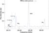 |
Fig. F.1 OH spectrum and nearby transitions of TiO2, HCN and SO2 observed in the range 265.65 to 266.05 GHz toward omi Cet (Mira). The frequencies of the two hyperfine transitions of OH in the υ = 0, J = 35/2 rotational level are indicated with two light green vertical lines. The F' – F'' = 17 – 17 hyperfine transition of the J = 35/2 level is blended with the 24(2, 22) – 24(1, 23) transition of TiO2. This spectrum is extracted from a 0.″2×0.″2 region containing all the OH emission. |
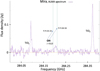 |
Fig. F.2 Line spectrum in the vicinity of the υ = 0, J = 31/2 rotational level of OH and of two nearby TiO2 transitions observed in the 284.00 to 284.40 GHz range toward omi Cet (Mira). The expected F' – F'' = 15–15 and 16 – 16 hyperfine transitions of OH in the J = 31/2 Λ-doublet are indicated with two light green vertical lines at the expected frequencies. The two TiO2 lines correspond to the 27(7, 21) – 27(6, 22) and 21(1, 21) – 26(0, 20) transitions at 284.0943 and 284.3719 GHz, respectively. Spectrum extracted from a 0.″25×0.″20 region containing all the OH emission. |
References
- Agúndez, M., Martínez, J. I., de Andres, P. L., et al. 2020, A&A, 637, A59 [CrossRef] [EDP Sciences] [PubMed] [Google Scholar]
- Alcolea, J., & Menten, K.M. 1993, in Astrophysical Masers, eds. A. W. Clegg, & G. E. Nedoluha (Berlin: Springer), 412, 399 [NASA ADS] [CrossRef] [Google Scholar]
- Alcolea, J., Bujarrabal, V., Planesas, P., et al. 2013, A&A, 559, A93 [NASA ADS] [CrossRef] [EDP Sciences] [Google Scholar]
- Amano, T., & Scappini, F. 1991, Chem. Phys. Lett., 182, 93 [NASA ADS] [CrossRef] [Google Scholar]
- Andresen, P., Tiesen, T., Spieker, H., et al. 2000, J. Mol. Spectrosc., 200, 277 [NASA ADS] [CrossRef] [Google Scholar]
- Andriantsaralaza, M., Ramstedt, S., Vlemmings, W. H. T., et al. 2022, A&A, 667, A74 [NASA ADS] [CrossRef] [EDP Sciences] [Google Scholar]
- Asaki, Y., Maud, L.T., Fomalont, E.B., et al. 2020, ApJS, 247, 23A [NASA ADS] [CrossRef] [Google Scholar]
- Barlow, M. J., Nguyen-Q-Rieu, Truong-Bach, et al. 1996, A&A, 315, L241 [NASA ADS] [Google Scholar]
- Baudry, A., & Diamond, P. 1998, A&A, 331, 697 [NASA ADS] [Google Scholar]
- Baudry, A., Desmurs, J. F., Wilson, T. L., et al. 1997, A&A, 327, 255 [NASA ADS] [Google Scholar]
- Baudry, A., Herpin, F., Humphreys, E. M. L., et al. 2018a, The Messenger, 171, 37 [NASA ADS] [Google Scholar]
- Baudry, A., Humphreys, E. M. L., Herpin, F., et al. 2018b, A&A, 609, A25 [NASA ADS] [CrossRef] [EDP Sciences] [Google Scholar]
- Baulch, D. L., Cobos, C. J., Cox, R. A., et al. 1992, J. Phys. Chem. Ref. Data, 21, 411 [NASA ADS] [CrossRef] [Google Scholar]
- Bergman, P., & Humphreys, E. M. L. 2020, A&A, 638, A19 [NASA ADS] [CrossRef] [EDP Sciences] [Google Scholar]
- Bladh, S., Liljegren, S., Höfner, S., et al. 2019, A&A, 626, A100 [NASA ADS] [CrossRef] [EDP Sciences] [Google Scholar]
- Boulangier, J., Gobrecht, D., Decin, L., et al. 2019, MNRAS, 489, 4890 [CrossRef] [Google Scholar]
- Brooke, James S. A., Bernath, Peter F., Western, Colin M., et al. 2016, J. Quant. Spectrosc. Radiat. Transf., 168, 142 [NASA ADS] [CrossRef] [Google Scholar]
- Bujarrabal, V., Alcolea, J., Mikolajewska, J., et al. 2013, A&A, 559, A93 [NASA ADS] [CrossRef] [EDP Sciences] [Google Scholar]
- Cernicharo, J., Alcolea, J., Baudry, A., & Gonzalez-Alfonso, E. 1997, A&A, 319, 607 [Google Scholar]
- Cherchneff, I. 2006, A&A, 456, 1001 [NASA ADS] [CrossRef] [EDP Sciences] [Google Scholar]
- Cheung, A. C., Rank, D. M., Townes, C. H., et al. 1969, Nature, 221, 626 [NASA ADS] [CrossRef] [Google Scholar]
- Collison, A. J., & Nedoluha, G. E. 1994, ApJ, 422, 193 [NASA ADS] [CrossRef] [Google Scholar]
- Condon, J. J. 1997, PASP, 109, 166 [NASA ADS] [CrossRef] [Google Scholar]
- Cotton, W. D., Mennesson, B., Diamond, P. J., et al. 2004, A&A, 414, 275 [NASA ADS] [CrossRef] [EDP Sciences] [Google Scholar]
- Coudert, L. H., Martin-Drumel, M.-A., & Pirali, O. 2014, J. Mol. Spectrosc., 303, 36 [NASA ADS] [CrossRef] [Google Scholar]
- Danchi, W. C., Bester, M., Degiacomi, C. G., et al. 1994, AJ, 107, 1469 [NASA ADS] [CrossRef] [Google Scholar]
- Daniel, F., & Cernicharo, J. 2013, A&A, 553, A70 [NASA ADS] [CrossRef] [EDP Sciences] [Google Scholar]
- Danilovich, T., Bergman, P., Justtanont, K., et al. 2014, A&A, 569, A76 [NASA ADS] [CrossRef] [EDP Sciences] [Google Scholar]
- Danilovich, T., Van de Sande, P., Plane, J. M. C., et al. 2021, A&A, 655, A80 [NASA ADS] [CrossRef] [EDP Sciences] [Google Scholar]
- De Beck, E., Lombaert, R., Agúndez, M., et al. 2012, A&A, 539, A108 [NASA ADS] [CrossRef] [EDP Sciences] [Google Scholar]
- Decin, L., Justtanont, K., De Beck, E., et al. 2010, A&A, 521, L4 [CrossRef] [EDP Sciences] [Google Scholar]
- Decin, L., Richards, A. M. S., Danilovich, T., et al. 2018, A&A, 615, A28 [NASA ADS] [CrossRef] [EDP Sciences] [Google Scholar]
- Decin, L., Montargès, M., Richards, A. M. S., et al. 2020, Science, 369, 1497 [Google Scholar]
- de Jong, T. 1973, A&A, 26, 297 [NASA ADS] [Google Scholar]
- Drouin, B. J. 2013, J. Phys. Chem. A, 117, 10076 [NASA ADS] [CrossRef] [Google Scholar]
- Elitzur, M., Goldreich, P., & Scoville, N. 1976, ApJ, 205, 384 [NASA ADS] [CrossRef] [Google Scholar]
- Endres, C. P., Schlemmer, S., Schilke, P., et al. 2016, J. Mol. Spectrosc., 327, 95 [NASA ADS] [CrossRef] [Google Scholar]
- Etoka, S., & Diamond, P. 2004, MNRAS, 348, 34 [Google Scholar]
- Etoka, S., & Le Squeren, A. M. 2000, A&AS, 146, 179 [NASA ADS] [CrossRef] [EDP Sciences] [Google Scholar]
- Faure, A., & Josselin, E. 2008, A&A, 492, 257 [NASA ADS] [CrossRef] [EDP Sciences] [Google Scholar]
- Furtenbacher, T., Tóbiás, R., Tennyson, J., et al. 2020, J. Phys. Chem. Ref. Data, 49, 033101 [NASA ADS] [CrossRef] [Google Scholar]
- Gaia Collaboration (Vallenari, A., et al.) 2023, A&A, in press, https://doi.org/10.1051/0004-6361/202243940 [Google Scholar]
- Gobrecht, D., Cherchneff, I., Sarangi, A., et al. 2016, A&A, 585, A6 [NASA ADS] [CrossRef] [EDP Sciences] [Google Scholar]
- Gobrecht, D., Plane, J. M. C., Bromley, S. T., et al. 2022, A&A, 658, A167 [NASA ADS] [CrossRef] [EDP Sciences] [Google Scholar]
- Goldreich, P., & Kwan, J. 1974, ApJ, 191, 93 [NASA ADS] [CrossRef] [Google Scholar]
- Goldreich, P., & Scoville, N. 1976, ApJ, 205, 144 [NASA ADS] [CrossRef] [Google Scholar]
- Goldsmith, P. F., & Langer, W.D. 1999, ApJ, 517, 209 [NASA ADS] [CrossRef] [Google Scholar]
- Gonzalez-Alfonso, E., Cernicharo, J., Alcolea, J., et al. 1998, A&A, 334, 1016 [NASA ADS] [Google Scholar]
- Gottlieb, C. A., Decin, L., Richards, A. M. S., et al. 2022, A&A, 660, A94 [CrossRef] [EDP Sciences] [Google Scholar]
- Gray, M. D., Baudry, A., Richards, A. M. S., et al. 2016, MNRAS, 456, 374 [NASA ADS] [CrossRef] [Google Scholar]
- Gray, M. D., Etoka, S., Richards, A. M. S., et al. 2022, MNRAS, 513, 1354 [NASA ADS] [CrossRef] [Google Scholar]
- Grechko, M., Aseev, O., Rizzo, T. R., et al. 2012, J. Chem. Phys., 136, 244308 [NASA ADS] [CrossRef] [Google Scholar]
- Harvey, P. M., Bechis, K. P., Wilson, W. J., & Ball, J. A. 1974, ApJS, 27, 331 [NASA ADS] [CrossRef] [Google Scholar]
- Harvey-Smith, L., & Cohen, R. J. 2005, MNRAS, 356, 637 [Google Scholar]
- Harwit, M., & Bergin, E. A. 2002, ApJ, 565, L105 [NASA ADS] [CrossRef] [Google Scholar]
- Herpin, F., Baudry, A., Alcolea, J., & Cernicharo, E. 1998, A&A, 334, 1037 [Google Scholar]
- Hinkle, K. H. 1978, ApJ, 220, 210 [Google Scholar]
- Hinkle, K. H., & Barnes, T. G. 1979, ApJ, 227, 923 [Google Scholar]
- Hinkle, K. H., Scharlach, W. W. G., & Hall, D. N. B. 1984, ApJS, 56, 1 [CrossRef] [Google Scholar]
- Hirota, T., Kim, Mi Kyoung, & Honma, M. 2012, ApJ, 757, L1 [NASA ADS] [CrossRef] [Google Scholar]
- Hirota, T., Kim, Mi Kyoung, Kurono, Y., et al. 2014, ApJ, 782, L28 [NASA ADS] [CrossRef] [Google Scholar]
- Hoai, D.T., Anh, P.T., Tuyet Nhung, P., et al. 2021, J. Korean Astron. Soc., 54, 171H [NASA ADS] [Google Scholar]
- Höfner, S., & Olofsson, H. 2018, A&ARv, 26, 1 [Google Scholar]
- Homan, W., Montargès, M., Pimpanuwat, B., et al. 2020, A&A, 644, A61 [NASA ADS] [CrossRef] [EDP Sciences] [Google Scholar]
- Homan, W., Pimpanuwat, B., Herpin, F., et al. 2021, A&A, 651, A82 [NASA ADS] [CrossRef] [EDP Sciences] [Google Scholar]
- Hudson, E. R., Lewandowski, H. J., Sawyer, B. C., & Ye, J. 2006, Phys. Rev. Lett., 96, 143004 [NASA ADS] [CrossRef] [Google Scholar]
- Humphreys, E. M. L. 2007, IAU Symp., 242, 471 [NASA ADS] [CrossRef] [Google Scholar]
- Hunter, T. R., Young, K. H., Christensen, R. D., & Gurwell, M. A. 2007, IAU Symp., 242, 481 [CrossRef] [Google Scholar]
- Ireland, M. J., Scholz, M., & Wood, P. R. 2011 MNRAS, 418, 114 [Google Scholar]
- Justtanont, K., Bergman, P., Larsson, B., et al. 2005, A&A, 439, 627 [NASA ADS] [CrossRef] [EDP Sciences] [Google Scholar]
- Justtanont, K., Khouri, T., Maercker, M., et al. 2012, A&A, 537, A144 [NASA ADS] [CrossRef] [EDP Sciences] [Google Scholar]
- Kaminski, T., Gottlieb, C. A., Young, K. H., et al. 2013, ApJS, 209, 38 [CrossRef] [Google Scholar]
- Kervella, P., Homan, W., Richards, A. M. S., et al. 2016, A&A, 596, A92 [NASA ADS] [CrossRef] [EDP Sciences] [Google Scholar]
- Kervella, P., Decin, L., Richards, A. M. S., et al. 2018, A&A, 609, A67 [NASA ADS] [CrossRef] [EDP Sciences] [Google Scholar]
- Khouri, T., de Koter, A., Decin, L., et al. 2014, A&A, 570, A67 [NASA ADS] [CrossRef] [EDP Sciences] [Google Scholar]
- Khouri, T., Vlemmings, L., Ramstedt, S., et al. 2016, MNRAS, 463, L74 [NASA ADS] [CrossRef] [Google Scholar]
- Khouri, T., Velilla-Prieto, L., De Beck, E., et al. 2019, A&A, 623, L1 [NASA ADS] [CrossRef] [EDP Sciences] [Google Scholar]
- Klos, J., Ma, Q., Dagdigian, P. J., et al. 2017, MNRAS, 471, 4249 [CrossRef] [Google Scholar]
- Knowles, S. H., Mayer, C. H., Cheung, A. C., et al. 1969, Science, 163, 1055 [NASA ADS] [CrossRef] [Google Scholar]
- Kolbe, W. F., Zollner, W. D., & Leskovar, B. 1981, Rev. Sci. Instrum., 52, 523 [NASA ADS] [CrossRef] [Google Scholar]
- Kondratko, P. T., Greenhill, L. J., & Moran, J. M. 2005, ApJ, 618, 618 [NASA ADS] [CrossRef] [Google Scholar]
- Lev, B. L., Meyer, E. R., Hudson, E. R., et al. 2006, Phys. Rev. A, 74, 061402 [NASA ADS] [CrossRef] [Google Scholar]
- Liljegren, S., Höfner, S., Nowotny, W., & Eriksson, K. 2016, A&A, 589, A130 [NASA ADS] [CrossRef] [EDP Sciences] [Google Scholar]
- Liljeström, T., Winnberg, A., & Booth, R. 1996, in URSI/IEEE/IRC XXI Convention on Radio Science, eds. P. Piironen, & A. Räisänen (Espoo: Helsinki University of Technology), 96 [Google Scholar]
- Lindqvist, M., Nyman, L.-A., Olofsson, H., et al. 1988, A&A, 205, L15 [Google Scholar]
- Maercker, M., Danilovich, T., Olofsson, H., et al. 2016, A&A, 591, A44 [NASA ADS] [CrossRef] [EDP Sciences] [Google Scholar]
- Martin-Drumel, M. A., Eliet, S., Pirali, O., et al. 2012, Chem. Phys. Lett., 550, 8 [CrossRef] [Google Scholar]
- Maud, L. T., Cesaroni, R., Kumar, M. S. N., et al. 2019, A&A, 627, L6 [NASA ADS] [CrossRef] [EDP Sciences] [Google Scholar]
- Melnick, G. J., Menten, K. M., Phillips, T.G., et al. 1993, ApJ, 416, L37 [NASA ADS] [CrossRef] [Google Scholar]
- Menten, K. M., & Melnick, G.J. 1989, ApJ, 341, L91 [NASA ADS] [CrossRef] [Google Scholar]
- Menten, K. M., & Young, K. 1995, ApJ, 450, L67 [NASA ADS] [CrossRef] [Google Scholar]
- Menten, K. M., Melnick, G. J., & Phillips, T. J. 1990a, ApJ, 350, L41 [NASA ADS] [CrossRef] [Google Scholar]
- Menten, K. M., Melnick, G. J., Phillips, T. G., et al. 1990b, ApJ, 363, L27 [NASA ADS] [CrossRef] [Google Scholar]
- Menten, K. M., Philipp, S. D., Güsten, R., et al. 2006, A&A, 454, L107 [NASA ADS] [CrossRef] [EDP Sciences] [Google Scholar]
- Montargès, M., Kervella, P., Perrin, G., et al. 2014, A&A, 572, A17 [NASA ADS] [CrossRef] [EDP Sciences] [Google Scholar]
- Montargès, M., Canon, E., de Koter, A., et al. 2023, A&A, 671, A96 [NASA ADS] [CrossRef] [EDP Sciences] [Google Scholar]
- Müller, H.S.P., Schlöder, F., Stutzki, J., et al. 2005, J. Mol. Spectrosc., 742, 215 [Google Scholar]
- Neufeld, D. A., & Melnick, G. J. 1991, ApJ, 368, 215 [NASA ADS] [CrossRef] [Google Scholar]
- Neufeld, D. A., Chen, W., Melnick, G. J., et al. 1996, A&A, 315, L237 [NASA ADS] [Google Scholar]
- Neufeld, D. A., González-Alfonso, E., Melnick, G., et al. 2011, ApJ, 727, L29 [NASA ADS] [CrossRef] [Google Scholar]
- Neufeld, D. A., Menten, K.M., Durán, C., et al. 2021, ApJ, 907, 42 [NASA ADS] [CrossRef] [Google Scholar]
- Nowotny, W., Höfner, S., Aringer, B. 2010 A&A, 514, A35 [NASA ADS] [CrossRef] [EDP Sciences] [Google Scholar]
- O’Gorman, E., Kervella, P., Harper, G. M., et al. 2017, A&A, 602, L10 [NASA ADS] [CrossRef] [EDP Sciences] [Google Scholar]
- Pearson, J. C. 1995, Ph.D. Thesis, Duke University, Durham, NC, USA [Google Scholar]
- Pearson, J. C., Anderson, T., Herbst, E., et al. 1991, ApJ, 379, L41 [NASA ADS] [CrossRef] [Google Scholar]
- Perrin, G., Ridgway, S. T., Mennesson, B., et al. 2004, A&A, 426, 279 [NASA ADS] [CrossRef] [EDP Sciences] [Google Scholar]
- Pickett, H. M. 1991, J. Mol. Spectrosc., 148, 371 [Google Scholar]
- Pickett, H. M., Poynter, R. L., Cohen, E. A., et al. 1998, J. Quant. Spectrosc. Radiat. Transf., 60, 883 [Google Scholar]
- Pickett, H. M., Pearson, J. C., & Miller, C. E. 2005, J. Mol. Spectrosc., 233, 174 [NASA ADS] [CrossRef] [Google Scholar]
- Polyansky, O. L., Kyuberis, A. A., Zobov, N. F., et al. 2018, MNRAS, 480, A56 [Google Scholar]
- Quintana-Lacaci, G., Velilla-Prieto, L., Agúndez, et al. 2023, A&A, 669, A53 [Google Scholar]
- Reid, M. J., & Menten, K. M. 1997, ApJ, 476, 327 [NASA ADS] [CrossRef] [Google Scholar]
- Reid, M. J., Muhleman, D. O., Moran, J. M., et al. 1977, ApJ, 214, 60 [NASA ADS] [CrossRef] [Google Scholar]
- Richards, A. M. S., Yates, J. A., & Cohen, R. J. 1999, MNRAS, 306, 954 [Google Scholar]
- Richards, A. M. S., Elitzur, M., & Yates, J. A. 2011, A&A, 525, A56 [NASA ADS] [CrossRef] [EDP Sciences] [Google Scholar]
- Richards, A. M. S., Etoka, S., Gray, M. D., et al. 2012, A&A, 546, A16 [NASA ADS] [CrossRef] [EDP Sciences] [Google Scholar]
- Richards, A. M. S., Impellizzeri, C. M. V., Humphreys, E. M., et al. 2014, A&A, 572, L9 [NASA ADS] [CrossRef] [EDP Sciences] [Google Scholar]
- Richter, L., Kemball, A., & Jonas, J. 2013, MNRAS, 436, 1708 [Google Scholar]
- Schoenberg, K. 1988, A&A, 195, 198 [NASA ADS] [Google Scholar]
- Schroeder, P. A. 2002, “IR spectroscopy”, in Clay Science in : CMS Workshop Lectures, 11, 181 [Google Scholar]
- Shostak, S. L., & Muenter, J. S. 1991, J. Chem. Phys., 94, 5883 [NASA ADS] [CrossRef] [Google Scholar]
- Shostak, S. L., Ebenstein, W. L., & Muenter, J. S. 1991, J. Chem. Phys., 94, 5875 [NASA ADS] [CrossRef] [Google Scholar]
- Spinrad, H., & Newburn, R. L., Jr. 1965, ApJ, 141, 965 [NASA ADS] [CrossRef] [Google Scholar]
- Tabone, B., van Hemert, M. C., van Dishoeck, E. W., et al. 2021, A&A, 650, A192 [NASA ADS] [CrossRef] [EDP Sciences] [Google Scholar]
- Takigawa, A., Kamizuka, T., Tachibana, S., et al. 2017, Sci. Adv., 3, eaao2149 [NASA ADS] [CrossRef] [Google Scholar]
- Tanaka, Kei E. I., Zhang, Yichen, Hirota, T., et al. 2020, ApJ, 900, L2 [NASA ADS] [CrossRef] [Google Scholar]
- Tappe, A., Lada, C. J., Black, J. H., et al. 2008, ApJ, 680, L117 [NASA ADS] [CrossRef] [Google Scholar]
- Tenenbaum, E. D., Dodd, J. L., Milam, S. N., et al. 2010, ApJ, 720, L102 [NASA ADS] [CrossRef] [Google Scholar]
- Teyssier, D., Quintana-Lacaci, G., Marston, A. P., et al. 2012, A&A, 545, A99 [NASA ADS] [CrossRef] [EDP Sciences] [Google Scholar]
- Tsuji, T. 1973, A&A, 23, 411 [NASA ADS] [Google Scholar]
- Tsuji, T., Ohnaka, K., Aoki, W., & Yamamura, I. 1997, A&A, 320, L1 [NASA ADS] [Google Scholar]
- van de Sande, M., & Millar, T. J. 2022, MNRAS, 510, 1204 [Google Scholar]
- van Dishoeck, E. F., Herbst, E., & Neufeld, D. A. 2013, Chem. Rev., 113, 9043 [Google Scholar]
- van Dishoeck, E.F., Kristensen, L. E., Mottram, J. C., et al. 2021, A&A, 648, A24 [NASA ADS] [CrossRef] [EDP Sciences] [Google Scholar]
- Velilla-Prieto, L., Sánchez Contreras, C., Cernicharo, J., et al. 2017, A&A, 597, A25 [NASA ADS] [CrossRef] [EDP Sciences] [Google Scholar]
- Vlemmings, W. H. T., Khouri, T., De Beck, E., et al. 2018, A&A, 613, L4 [NASA ADS] [CrossRef] [EDP Sciences] [Google Scholar]
- Vlemmings, W. H. T., Khouri, T., & Olofsson, H. 2019, A&A, 626, A81 [NASA ADS] [CrossRef] [EDP Sciences] [Google Scholar]
- Weinreb, S., Barrett, A. H., Meeks, M. L., & Henry, J. C. 1963, Nature, 200, 829 [NASA ADS] [CrossRef] [Google Scholar]
- Willacy, K., & Cherchneff, I. 1998, A&A, 330, 676 [NASA ADS] [Google Scholar]
- Wilson, W. J., & Barrett, A. H. 1968, Science, 161, 778 [NASA ADS] [CrossRef] [Google Scholar]
- Winters, J. M., Hoai, D. T., Wong, K. T., et al. 2022, A&A, 658, A135 [CrossRef] [EDP Sciences] [Google Scholar]
- Wong, K. T., Kaminski, T., Menten, K. M., & Wyrowski, F. 2016, A&A, 590, A127 [NASA ADS] [CrossRef] [EDP Sciences] [Google Scholar]
- Yates, J. A., Field, D., & Gray, M. D. 1997, MNRAS, 285, 303 [NASA ADS] [Google Scholar]
- Yu, S., Pearson, J. C., Drouin, B. J., et al. 2012, J. Mol. Spectrosc., 279, 16 [NASA ADS] [CrossRef] [Google Scholar]
- Yu, S., Pearson, J. C., & Drouin, B. J. 2013, J. Mol. Spectrosc., 288, 7 [NASA ADS] [CrossRef] [Google Scholar]
DR3 measurements are robust, although photospheric structures could affect the photocenter position. Data processing of the next data release will be improved with more astrometric measurements.
Further calculations of the OH rotational spectra in υ = 0 to 2 are given in the CDMS catalog (Müller et al. 2005; Endres et al. 2016). OH entries and our fit results and line list with frequencies from the radio astronomy observations are available from https://cdms.astro.uni–koeln.de/classic/entries/archive/OH/
Our Band 6 uniform disk sizes are 13.5 and 17.2 mas for AH Sco and VX Sgr, respectively. In Betelgeuse the radio continuum diameter (O’Gorman et al. 2017) and the IR/optical diameter (Montargès et al. 2014) are 58 and 42 mas, respectively.
SAD (Search And Destroy) enables to search for potential sources within an image and fits Gaussian components. It is useful for the analysis of complex images provided that they contain compact enough emission (e.g., Etoka & Diamond 2004; Baudry & Diamond 1998).
It is worth adding that interpretation of the ALMA observations in terms of binarity is well documented in L2 Pup and π1 Gru (Kervella et al. 2016; Homan et al. 2020).
The ATOMIUM observations of U Her show extended thermal SiO emission in this SW blob. Extended emission in similar directions have also been observed in 22.235 GHz water masers over more than 24 yr (Richards et al. 2012).
VY CMa, IK Tau, and W Hya, not included in our survey, also exhibit emission at both 658.007 GHz (e.g., Hunter et al. 2007; Baudry et al. 2018b), and 268.149 GHz (Tenenbaum et al. 2010; Velilla-Prieto et al. 2017; K. Ohnaka & K.T. Wong, priv. comm.)
The 658.01 GHz high angular resolution mapping of Asaki et al. (2020) delineates a probable shock front around “clump” C which could have been ejected from the central star, thus highlighting the unusual nature of VY CMa.
Besides evolved stars, the 232.687 GHz line (not in our set-up) in the (0,1,0) state was observed with ALMA in Orion (e.g., Hirota et al. 2012) and in two other star forming regions (Maud et al. 2019; Tanaka et al. 2020). Liljeström et al. (1996) also observed the 96.261 GHz transition in the (0,1,0) state toward two young stellar objects.
Excitation by electrons is expected to be small in AGBs. The mole fraction of electrons estimated from the equilibrium thermochemical data of Agúndez et al. (2020) is ≲5 × 10⁻⁶. The CODEX models (Ireland et al. 2011), better suited to a dynamic atmosphere, provide an electron content below 10−5 except very close to the star where water is not excited.
Bergman & Humphreys (2020) suggest that line overlap between the two H2O species could explain the strong maser observed in evolved stars around 437.347 GHz in the (0,0,0) state.
This suggests that simultaneous observation of these lines would help to identify nonthermal emission in at least one line if the line intensity ratio deviates from the LTE conditions.
In the near IR, however, the OH vibration-rotation overtone bands have long been known in Mira variables; for more details, readers can refer to the CO and OH bands in R Leo (Hinkle 1978), for example.
Our uniform disk sizes at 250 GHz are 27.1, 20.4, 15.0 and 20.0 mas for R Hya, S Pav, R Aql and T Mic, respectively. See also Sect. 4.3 for discussion on H2O angular sizes.
Note that mid-IR spectral resolution observations of the OH Λ-doubling up to J = 69/2 have been reported in the young protostellar outflow HH 211 (Tappe et al. 2008) and modeled (Tabone et al. 2021).
The approximate optical phases of our OH high resolution observations acquired in 2019 are: 0.8, 0.9, 0.2, 0.5 and 0.7 for R Hya, S Pav, R Aql, VX Sgr and AH Sco, respectively. The phase is not well defined in T Mic, but was ∼0.5.
In addition to our Band 6 survey, using the ALMA archival data, we also found J = 35/2, line 9 emission in Mira (Appendix F and Table 3).
We note that the J = 33/2 rotational level in the Χ2Π1/2 state of OH (E = 7960 K) is close in energy (within ≲400 K) to the rotational levels of three high-lying transitions of H2O which were observed in at least six stars in the ATOMIUM survey: line #1 in eight stars, line #8 in six stars, and line #13 in seven stars.
All Tables
Observable υ = 0 and 1, ΔJ = 0, ΔF = 0 transitions of OH in the ATOMIUM frequency line setting (excluding ΔF = ±1 and very high N, J transitions).
Frequencies of OH Λ-doubling transitions from astronomical observations and comparison with calculated frequencies.
H2O peak flux density (first entry in mJy) and velocity extent (second entry in km s−1, highlighted with italics) of observed lines for an aperture diameter of 0.′′08 extracted from the extended configuration.
Maximum brightness temperatures of ortho and para water at 268.149 and 262.898 GHz.
Dates of observations with the main and ACA arrays and associated optical phases (in parentheses) of the variable 268.149 GHz H2O sources.
Peak flux density, r.m.s. noise and angular size in zeroth moment maps of OH emission and absorption.
Observed integrated flux density and peak flux density ratios (Integr. ratio and Peak ratio) and LTE opacity ratio of OH hyperfine transitions in J = 27/2, 29/2, 33/2 and 35/2.
Peak surface brightness (Sp), peak brightness temperature (Tb) and uncertainty in the J = 27/2 and 29/2 rotational levels of OH.
Quantum numbersa, transition frequency (Frequency), uncertainty (Unc.), lower state energy (Elow) and A value of OH Λ-doubling transitions in the υ = 0, 2Π3/2 state from our present fit.
Quantum numbersa, transition frequency (Frequency), uncertainty (Unc.), lower state energy (Elow) and A value of OH Λ-doubling transitions in the υ = 0, 2Π1/2 state from our present fit.
Quantum numbersa, transition frequency (Frequency), uncertainty (Unc.), lower state energy (Elow) and A value of OH Λ-doubling transitions in the υ = 1, 2Π3/2 state from our present fit.
Quantum numbersa, transition frequency (Frequency), uncertainty (Unc.), lower state energy (Elow) and A value of OH Λ-doubling transitions in the υ = 1, 2Π1/2 state from our present fit.
All Figures
|
Fig. 1 Three fundamental vibrational modes of water vapor. They are denoted v1 and v3 for the symmetric and asyimrietric stretchings, and v2 for the symmetric bending. The arrows simulate me direct and reciprocal vibrational motions of the Ο and the two H atoms (adapted from Schroeder 2002). The Ο to Η bond length is nearly 0.1 nm and the H-O-H average angle is 104°. The a and b axes discussed in Sect. 3.1 intersect at the center of mass of the molecule. The energy of the three fundamental vibrational states v1 ν2, v3 are 3657, 1595 tind 3756 cm−1, respectively; the equivalent stale temperature and warelengths are 5262, 2294 and 5404 K (see also Fig. 2) and 2.73, 6.27 and 2.66 μm. |
| In the text | |
|
Fig. 2 Lowest eight vibrational s)atei of water vapor and their quantum numbers (υ1,υ2,υ3). Stares of a1 symmetry are referred to by horizontal blue lines, states of b2 symmetry by aubergine lines. Vibration-rotation interactions are indicated by lines connecting the interacting states. The labels F, C and C’ symbolize Fermi, Coriolis, and rotational (or Coriolis-type) interactions. The energy of each vibrational band origin is given in Kelvin below each horizontal solid line. The rotational and ro-vibrational transitions in the range of snerau covered by the ATOMIUM project are listed in Table 2. Four examples, corresponding to lines 10, 14, 8 and 4 in Table 2, are shown with their quantum identification, in the form on dotted horizontal green lines; they are ordered by increasing energy. |
| In the text | |
|
Fig. 3 Water line profiles extracted from the extended configuration of the main array for an aperture diameter of 0.′′08 in R Hya. First two rows: six transitions of ortho H2O as defined in Table 2: lines 1, 6, 8 (including line 7 separated by 12.7 MHz, or 15.0 km s−1, from line 8) and lines 13 and 14. Last row: two transitions of para H2O as defined in Table 2: lines 10 and 12. The spectra are converted from the observed frequency to the LSR frame using the H2O catalog Une rest frequencies given in Table 2. In all spectra, the blue vertical line indicates the adopted new LSR systemic velocity as shown in Table1. For line 1 (upper left panel), file red verticad line shows the LSR velocity for the slightly different frequency determined in this work. Spectral resolution varies from ~1.1 km s−1 (268 GHz) to ~1.3 (222 GHz) km s−1. |
| In the text | |
|
Fig. 4 Typical line profiles of the (0,3,0) 83,6 – 74,3 transition of H2O at 222.014 GHz in R Aql, S Pav, IRC+10011 and VX Sgr. The upper left panel in Fig. 3 shows the same transition in R Hya. Spectra are extracted for an aperture diameter of 0.′′ 08 from the extended configuration and converted from the observed frequency to the LSR frame using the H2O catalog; line rest frequency given in Table 2. The red and blue vertical lines indicate the new LSR systemic velocity (see Table 1) corresponding to our frequency determination and to the catalog frequuncy, respectively. The spectral resolution is ~1.3 km s−1. |
| In the text | |
|
Fig. 5 Absorption spectra of para H2O at 244.330 GHz in R Hya, S Pav and RAql (blue profiles) and, emission/absorption spectra of the υ = 1 transition of CO(2−1) at 228.439 GHz in the same sources (red profiles). The spectra are converted from the observed frequency to the LSR systemic velocity using the H2O line 5 (Table 2) and υ = 1, CO(2−1) rest frequencies. All spectra are extracted from the high resolution data cubes for an aperture diameter of 0.′′08. The vertical black dotted lines indicate the adopted new LSR systemic velocities (see Table 1). |
| In the text | |
|
Fig. 6 High resolution channel maps of H2O (0,2,0) 65,2–74,3 transition at 268.149 GHz in R Hya and U Her. Each map (R Hya and U Her, left and right panels) shows offsets in the R.A. and Dec. directions which we call throughout this work “Relative RA” and “Relative Dec”. The corresponding angular offsets cover 100 × 100 mas from the continuum emission peak at (0,0) position (coordinates given in Table 1). Each channel velocity is in the LSR frame from −23.9 to 2.3 km s−1 (R Hya) and −28.6 to −2.3 km s−1 (U Her). White light contours are at −3, 3 and 5σ. A few negative contours, when present, are dashed. The line peak and typical rms noise are 65 and 1 mJy beam−1 (R Hya), and 122 and 1.5 mJy beam−1 (U Her). The red contour at (0,0) delineates the extent at half peak intensity of the continuum emission. We characterize the elliptical Gaussian clean beams by their major and minor axes and position angle (PA) at half power, hereafter HPBW clean beam parameters. For the line observations of R Hya and U Her, these are (38 × 29) mas at PA 48° and (26 × 19) mas at PA 11°, respectively. The corresponding continuum parameters are (34 × 25) mas at PA 67° for R Hya and (24 × 18) mas at PA 8° for U Her. The line and continuum beams are shown at the bottom left of each map in white and solid dark-red, respectively. The scale of the line flux density per beam (in mJy beam−1) is linear and shown in the vertical bar on the right side of each channel map. |
| In the text | |
|
Fig. 7 High resolution channel maps of the (0,0,1) 31,3–22,0 and (0,2,0) 143,12–134,9 transitions of water near 254 GHz in R Hya. The upper and lower panels correspond tothe 254.040 GHz and 254.053 GHz transitions, respectively (lines 7 and 8 in Table 2). Caption as in Fig. 6 except for the velocity range and the line peak, 8 mJy/beam; the typical r.m.s. noise is 1 mJy/beam. The HPBW is (39 × 30) mas at PA 49° and (34 × 25) mas at PA 67° for the line and continuum, respectively. |
| In the text | |
|
Fig. 8 Zeroth moment absorption maps of the (1,1,0)–(0,1,1) |
| In the text | |
|
Fig. 9 Comparison of absorption and emission lines of water with υ = 1, CO(2–1) absorption in R Hya. Left: panel: Magenta and cyan dashed contours delineate the −5σ levels of the 244.330 GHz (line 5) and 259.952 GHz (line 10) mom 0 absorption maps. The underlying map is the mom 0 absorption map of υ = 1, CO(2−1) with the yellow dashet contour at the −3σ level. The line beam width is 550 × 28 mas with 70° orientation (white ellipse in bottom left corner The red solid contour delineates the 50% level of the peak continuum emission (the continuum beam width is the dark-red ellipse in the bottom left corner). Right panel: the magenta dashed contour and red solid contour indicate the 244.330 GHz absorption and mm-wave continuum emission as in the left panel. The underlying map is the 259.952 GHz mom 0 emission, with the white solid contours at the 20 and 35σ levels. (Line and continuum beam widths as in the left panel.) The noise level is 3 mJybeam−1 km s−1 for water in both panels and 4.3 mJy/beam km s−1 for CO. The velocity intervals of the mom 0 maps are: −13.2 to 4.3 and −2.3 to t.5 km s−1 for the 244.330 and 259.952 GHz absorptions; −18.8 to −3.0 km s−1 for the 259.952 GHz emission of water; −2.2 to 6.0 km s−1 for the CO(2−1) absorption. |
| In the text | |
|
Fig. 10 Maps of the different velocity components of water identified in the Gaussian-fit procedure at 268.149 and 262.898 GHz toward R Hya and UHer for the extended configuration of the main array. The size of the colored symbols varies as the square root of the integrated flux density of the Gaussian component; the crosses show the position uncertainty for each component The velocity scale colors are given on the right side of each map with respect to the stellar system velocity taken to be −10.1 and −14.9 km s−1 in the LSR frame for R Hya and U Her, respectively. The dashed gray circle represents the size of the optical photosphere (23.7 and 11.2 mas for R Hya and U Her, respectively) and the larger gray circle represents the 250 GHz continuum emission size (27.1 and 188.5 mat for RHya and U Her). |
| In the text | |
|
Fig. 11 Population diagrams for ortho and para H2O transitions (black and red numbers, respectively) in R Hya, S Pav, AH Sco and IRC+10011. The number near each data point corresponds to the numbering used to identify each line in Table 2. The vertical bar in each data point includes the ±1σ formal error of the integrated flux density and a rough estimate of the filling factor uncertainty. The green line is the regression line across the data points from which the rotationaf temperature and the column density are derived (see Sect. 5.2). The strong 268.149 GHz maser line (line 14) is excluded from the IRC+10011 and AH Sco plots while it is kept in R Hya and S Pav. |
| In the text | |
|
Fig. 12 Comparison of the 268.149 GHz line profiles in U Her observed with the mid configuration of the main array in Oct 2018 and Aug 2019 (blue and red curves, respectively). The spactra are extracted for an aperture diameter of 0.″4; the Spectral resolution is ∼1 km s−1. The vertical line shows the systemic stellar velocity. The mom 0 emission maps at these two epochs are presented in Fig. 14. |
| In the text | |
|
Fig. 13 Comparison of the 268.149 GHz line profiles extracted for an aperture diameter of 0.″4 in VX Sgr observed at ∼1 km s−1 resolution in November 2018 and July 2019 with the mid and extended configurations of the main array (upper and lower panels, respectively). The weak feature near −20 km s−1 in the 2019 spectrum corresponds to the ν = 0, JKa,Kc = 95,5−104,6 transition oO SO2 at 268168.335 MHz; it is also barely seen in the 2018 mid spectrum. The vertical lines are at the adopted new LSR systemic velocity. |
| In the text | |
|
Fig. 14 Zeroth moment maps of the 268.149 GHz emission of water in U Her obtained with the mid configuration of the main array at two different epochs, 2018, Oct. 14 and 2019, Aug. 24. The emission is integrated over the −21.6 to −9 km s−1 velocity range. The 2019 image has been convolved with the larger 2018 image beam shown in the lower lrft of each panel (0.″21 × 0.″18). In both maps the noise is 0.02 Jy beam−1 km s−1 and the 5σ emission contour is shown as a white light: contour. The map maxima are 21.6 and 1.67 Jybeam−1 km s−1 in 2018 and 2019), respectively. The small red contour at the image center is the 50% continuum emission from the high resolution data. Note the SW blob emission in the 2018 map (see Sect. 6.1.1). |
| In the text | |
|
Fig. 15 Comparison of the 268.149 GHz line profiles in GY Aq1 and R Aql observed with the ACA and the mid and extended main array configurations. The ACA spectral resolution has been degraded here to 2 and 0.5 km s−1 (GY Aql and R Aql, respectively) for comparison with the ~1 km s−1 resolution of the mid and extended configurations of the main array. The epoch of the observations are indicated in the figure labels as well as the diameter of the extraction aperture given in parentheses (18.″0, 0.″4 and 0.″2 for GY Aql and 18.″0, 1.″0 and 0.″1 for R Aql). The vertical lines show the systemic stellar velocity. |
| In the text | |
|
Fig. 16 Comparison of the 262.898 GHz line profiles in IRC+10011 observed at different epochs with the mid, extended and compact configurations of the main array. The epoch of the observations and the diameter of the extraction apertures (4″.0, 0″.4 and 0″.15) are shown in the figure labels. The spectral resolution is ~1.1 km s−1. The vertical line shows the systemic stellar velocity. |
| In the text | |
|
Fig. 17 Comparison of maser depths of ortho H2O at 268.149 and 658.007 GHz (upper and lower two panels) using models in Gray et al. (2016). Strong maser emission at 268.149 and 658.007 GHz is obtained for markedly different kinetic temperatures (vertical axis on left hand-side of each panel) and dust temperatures Td (given in the upper right-hand side of each panel). The transition frequency is given in the upper left corner of each panel with, below the letter o for ortho H2Ο followed by the vibrational stale fnd the rotational transition. The negative optical depth is specified in the vertical bar on the right-hand side of each panel using a log normal scale (min = −0.1 and max = −75.0); black means no inversion. The molecular H2 density is obtained by dividing the water abundance by 3 × 10⁻⁵.) |
| In the text | |
|
Fig. 18 Negative optical depths as in Fig. 17 at 262.898 and 263.451 in the (010) vibrational state. The quantum numbers of these transitions are preceded by the letters ρ and ο for para and ortho H20. (The molecular H2 density is obtained by dividing the water abundance by 3 × 10⁻⁵.) |
| In the text | |
|
Fig. 19 R Hya spectra of the F′ − F″ = 13−13 and 14−14 hyperfine transitions of OH in the υ = 0, J = 27/2 rotational transition (lines 1 and 2 in Table 3) extracted from combined high and mid spatial resolution data for an aperture diameter of 0.″08, 0.″16 and 0.″40. The spectra are converted from the observed frequency to the LSR frame using the line 2 rest frequency as the “reference” frequency. The black dotted vertical line (line 2) is at the adopted new systemic velocity (see Table 1). The green dotted vertical line is displaced by ~24.3 km s−1 compared to line 2 as expected from the υ = 0, J = 27/2 Λ-doublet frequency separation; it corresponds to line 1. |
| In the text | |
|
Fig. 20 Spectra of R Hya, S Pav and R Aql in the J = 27/2 and 29/2 rotational levels of OH extracted from the high resolution data cubes for an aperture diameter of 0/08. The three left and three right panels correspond to J = 27/2 and 29/2, respectively. In each spectrum, the two nearby emission features correspond to the two hyperfine transitions of each A-doublet (dotted blue and red vertical lines). Note weak absorption features observed in all six spectra. In the J = 29/2 spectra, the most negative velocity emission feature (closest to the F′ – F″ = 15–15 transition) is the 252.172 GHz line of water. The spectra are converted from the observed frequency to the LSR frame using the OH catalog line rest frequencies given in Table 3. Line 2 at 221353.48 MHz and line 8 at 252145.35 MHz are taken as the reference frequencies for each spectrum in the J = 27/2 and 29/2 states; they are placed at the adopted new systemic velocities (see Table 1). |
| In the text | |
|
Fig. 21 High resolution channel maps of J = 29/2, F′ – F″= 14 – 14 and 15–15 transitions of OH in R Hya (upper and lower panels, respectively). Each map covers 200 × 200 mas and is centered on the continuum emission peak at (0,0) position (coordinates given in Table 1). Each channel velocity is in the LSR frame using the OH catalog rest frequency in Table 3. The white contours are at −3, 3 and 5σ. The line peak flux density and the typical r.m.s. noise are 9 mJy beam−1 and 1 mJy beam−1, respectively. The red contour delineates the extent at half peak intensity of the continuum emission. The line and continuum beams are shown at the bottom left of each map in white and dark-red, respectively. The HPBW is (39 × 31) mas at PA 46° and (34 × 25) mas at PA 67° for line and continuum, respectively. |
| In the text | |
|
Fig. 22 Zeroth moment map of OH emission in the J = 29/2, F′ – F″ = 14–14 and 15–15 transitions. Left panels: F′ – F″ = 14–14 transition in R Hya and S Pav. Right panels: F′ – F″ = 15–15 transition in the same sources. Offsets in RA and Dec directions are relative to the coordinates of the peak: stellar continuum as given in Table 1. The velocity intervals in the F′ – F″ = 14–14 and 15–15 transitions are: −11.8 to −2. 6 km s−1 and −12.2 to −1.7 km s−1 in R Hya; −21. 1 to −13.8 km s−1 and −21.2 to −11.9 km s−1 in S Pav. In each map the white contours are at 3 and 5σ. The red contour delineates the extent at half peak intensity of the continuum emission. The line and continuum beams are shown at. the bottom left of each map in white and dark-red, respectively. The line HPBW in R Hya is as in Fig. 21; in S Pav the line HPBW is (25 × 20) mas at PA 11°. The continuum beam is (34 × 25) mas at PA 67° (R Hya) and (25 × 20) mas at PA −13° (S Pav). |
| In the text | |
|
Fig. 23 Zeroth moment map of OH absorption in the J = 27/2, F′ – F″ = 14–14 and 13–13 transitions. Leftpanels: F′– F″ = 14–14 transition in R Aql and S Pav. Right panels: F′ – F″ = 13–13 transition in the same sources. Offsets in RA and Dec. directions are relative to the coordinates of the peak stellar− continuum as given in Tattle 1. The velocity intervals in the F′ – F″ = 14–14 and 13–13 transitions are: 55.8 to 61.2 km s−1 and 56.2 to 66.2 km s−1 in R Aql; −10.2 to −3.6 km s−1 and −9.4 to 33.5 km s−1 in S Pav The dotted white contours are at −33 and −5σ The red contour delineates the extent at half peak intensity of the continuum emission. The line and continuum beams are shown at the bottom left of each map in white and dark-red, respectively. The line HPBW is (27 × 22 mas) at PA 18° and (27 × 21) mas at PA −3° in R Aql and S Pav, respectively. The continuum beam is (24 × 22 mas at: PA −13 (R Hya) and (25 × 20) mas at PA −13° (S Pav). |
| In the text | |
|
Fig. 24 OH population diagram for R Hya, S Pav and R Aql. The number near each data point is the line number used in Table 3 of observable OH transitions. The vertical bar in each data point includes the ±1σ formal error of the integrated flux density and a rough estimate of the filling factor uncertainty. (An arrow indicate an upper limit.) Τhe green line is the regression line across the data points (see Sect. 9.2). |
| In the text | |
|
Fig. 25 Model predictions of the OH/H2O abundance ratio versus the radial distance at different pulsation phases of Mira-type and semi-regular variables. The spread in the abundance ratio versus the radial distance and the optical phase is discussed in Sect. 10. |
| In the text | |
|
Fig. B.1 Spectra of line 1 at 222.014 GHz (Table 2) extracted from the extended configuration array. The extraction diameter (in arc sec) is given in parentheses below the source name in the upper left corner of each spectrum. The observed frequency is converted to the LSR frame using the catalog line rest frequency given in Table 2. The blue vertical line indicates the adopted new LSR systemic velocity (see Table 1). The red vertical line shows the LSR velocity for the slightly different frequency determined in this work (see Table 2). |
| In the text | |
|
Fig. B.2 Spectra of line 5 at 244330 GHz (Table 2) extracted from the extended configuration array. The extraction diameter (in arc sec) is given in parentheses below the source name in the upper left corner of each spectrum. The observed frequency is converted to the LSR frame using the catalog line rest frequency given in Table 2. The blue vertical line indicates the adopted new LSR systemic velocity (see Table 1) |
| In the text | |
|
Fig. B.3 Spectra of line 6 at 252.172 GHz (Table 2) extracted from the extended configuration array. The rest of the figure caption is as in Fig. B.2. |
| In the text | |
|
Fig. B.4 Spectra of lines 7 and 8 at 254.040 and 254.053 GHz (Table 2) extracted from the extended configuration array. The extraction diameter (in arc sec) is given in parentheses below the source name in the upper left corner of each spectrum. The blue and red vertical lines (lines 7 and 8) indicate the adopted new LSR systemic velocity (see Table 1) using the catalog rest frequencies (Table 2). |
| In the text | |
|
Fig. B.5 Spectra of line 10 at 259.952 GHz (Table 2) extracted from the extended configuration array. The rest of the figure caption is as in Fig. B.2.. |
| In the text | |
|
Fig. B.6 Spectra of line 12 at 262.898 GHz (Table 2) extracted from the extended configuration array. The rest of the figure caption is as in Fig. B.2. |
| In the text | |
|
Fig. B.7 Spectra of line 13 at 266.574 GHz (Table 2) extracted from the extended configuration array. The rest of the figure caption is as in Fig. B.2. |
| In the text | |
|
Fig. B.8 Spectra of line 14 at 268.149 GHz (Table 2) extracted from the extended configuration array. The rest of the figure caption is as in Fig. B.2. |
| In the text | |
|
Fig. B.9 Spectra of line 12 at 262.898 GHz (Table 2) extracted from the mid configuration array. The rest of the figure caption is as in Fig. B.2. |
| In the text | |
|
Fig. B.10 Spectra of line 14 at 268.149 GHz (Table 2) extracted from the mid configuration array. The rest of the figure caption is as in Fig. B.2. |
| In the text | |
|
Fig. C.1 Spectrum of the (0,0,1) 143,12–134,9 transition of para H2O in R Hya (upper panel). Following the IPL catalog, we assume a rest frequency of 236.8054 GHz (line 4 in Table 2). The line profiles are extracted from the combined high and mid resolution data cubes for circular apertures with 0.″708, 0.″12 and 0.″16 diameters. The vertical dashed line marks the water line frequency shifted by the systemic velocity of the star |
| In the text | |
|
Fig. C.2 Emission line profiles toward AH Sco (blue) and VX Sgr (red) in the vicinity of the υ = 0, J = 6–5 transition of 30SiO (at 254.217 GHz) and of the (0,1,1) 73,4–(l, 1,0) 65,1 transition of para water near 254.235 GHz (line 9, Table 2). The spectra are extracted from the high resolution data for a circular aperture of 0.″2 diameter and plotted in the rest frequency frame. The dotted black vertical line is the expected water frequency according to Furtenbacher et al. (2020) (see Table 2). Identification of the water transition at 254.235 GHz is uncertain (see discussion in Appendix C). |
| In the text | |
|
Fig. D.1 High resolution channel map of S Pav in the (0,2,0) 65,2−74,3 rotational transition of water at 268.149 GHz. Caption as in Fig. 6 except for the velocity range and the line peak flux density, 75 mJy/beam; the typical r.m.s. is 1 mJy/beam. The HPBW is (23×18) mas at PA 4° and (25×20) mas at PA –13° for the line and continuum, respectively. |
| In the text | |
|
Fig. D.2 High resolution channel map of IRC+10011 in the (0,2,0) 65,2−74,3 rotational transition of water at 268.149 GHz. Caption as in Fig. 6 except for the velocity range and the line peak flux density, 1178 mJy/beam; the typical r.m.s. is 2 mJy/beam. The HPBW is (24×19) mas at PA 26° and (27×19) mas at PA 31° for the line and continuum, respectively. |
| In the text | |
|
Fig. D.3 High resolution channel map of VX Sgr in the (0,2,0) 65,2–74,3 rotational transition of water at 268.149 GHz. Caption as in Fig. 6 except for the velocity range and the line peak flux density, 263 mJy/beam; the typical r.m.s. is 2 mJy/beam. The HPBW is (33×21) mas at PA 89° and (28×20) mas at PA 89° for the line and continuum, respectively. |
| In the text | |
|
Fig. D.4 High resolution channel map of AH Sco in the (0,2,0) 65,2–74,3 rotational transition of water at 268.149 GHz. Caption as in Fig. 6 except for the velocity range and the line peak flux density, 60344 mJy/beam; the typical r.m.s. is 1 mJy/beam. The HPBW is (40×23) mas at PA 38° and (23×23) mas at PA 70° for the line and continuum, respectively. |
| In the text | |
|
Fig. D.5 High resolution channel maps of R Hya and U Her in the (0,1,0) 77,1–86,2 rotational transition of water (line 12) at 262.898 GHz (upper and lower panels). Caption as in Fig. 6 except for the line frequency, velocity range and the line peak flux density, 20.9 mJy/beam (R Hya) and 16.7 mJy/beam (U Her); the typical r.m.s. is 1 mJy/beam in both stars. The line HPBW is (47×27) mas at PA 73° (R Hya) and (28×20) mas at PA 20° (U Her). The continuum HPBW is (34χ25) mas at PA 67° (R Hya) and (24×18) mas at PA 8° (U Her). |
| In the text | |
|
Fig. D.6 High resolution channel map of S Pav and IRC+10011 in the (0,1,0) 77,1–86,2 rotational transition of water (line 12) at 262.898 GHz (upper and lower panels). Caption as in Fig. 6 except for the line frequency, velocity range and the line peak flux density, 12.8 mJy/beam (S Pav) and 31.5 mJy/beam (IRC+10011); the typical r.m.s. is 1 and 2 mJybeam−1, respectively. The line HPBW is (24×18) mas at PA −20° (S Pav) and (26×20) mas at PA 22° (IRC+10011). The continuum HPBW is (25×20) mas at PA −13° ( S Pav) and (27×19) mas at PA 31° (IRC+10011). |
| In the text | |
|
Fig. D.7 High resolution channel map of VX Sgr and AH Sco in the (0,1,0) 77,1–86,2 rotational transition of water (line 12) at 262.898 GHz (upper and lower panels). Caption as in Fig. 6 except for the line frequency, velocity range and the line peak flux density, 26 mJy/beam (VX Sgr) and 33.5 mJy/beam (AH Sco); the typical r.m.s. is 2 and 6.5 mJy/beam, respectively. The line HPBW is (30×22) mas at PA 80° (VX Sgr) and (45×36) mas at PA 59° (AH Sco). The continuum HPBW is (28×20) mas at PA 89° ( VX Sgr) and (23×23) mas at PA 70° (AH Sco). |
| In the text | |
|
Fig. D.8 High resolution channel maps of relatively low energy (3954 K or 2748 cm−1) (0,0,0) 136,8−143,11 transition of water at 259.952 GHz in R Hya and S Pav (upper and lower panels). Caption as in Fig. 6 except for the velocity range and the line peak flux density, 15 and 9 mJy/beam in R Hya and S Pav, respectively; the typical r.m.s. noise is 1 mJy/beam for both stars. The HPBW is (48×28) mas at PA 72° and (34×25) mas at PA 67° for the line and continuum in R Hya, respectively, and (24×19 mas) at PA −19° (line) and (25×20) mas at PA −13° (continuum) in S Pav. |
| In the text | |
|
Fig. D.9 High resolution channel maps of water at 259.952 GHz in IRC+10011 and VX Sgr (upper and lower panels). Caption as in Fig. 6 except for the velocity range and the line peak; flux density, 26.5 and 12.2 mJy/beam in IRC+10011 and VX Sgr, respectively; the typical r.m.s. noise is 1.7 mJy/beam (IRC+10011) and 1.5 mJy/beam (VX Sgr). The HPBW is (26×19) mas at PA 24° and (27×19) mas at PA 31° for the line and continuum in IRC+10011, respectively, and (30×22) mas at PA 79° (line) and (28×20) mas at PA = 89° (continuum) in VX Sgr. |
| In the text | |
|
Fig. D.10 High resolution channel maps of high energy (8331 K) (0,3,0) 83,6–74,3 transition of H2O at 222.014 GHz in R Hya and S Pav (upper and lower panels). Caption as in Fig. 6 except for the velocity range and the line peak flux density, 9.3 and 6.5 mJy/beam in R Hya and S Pav, respectively; the typical r.m.s. noise is ~1 mJy/beam in both stars. The LSR velocity in each panel is determined from our own rest frequency, 222017.31 MHz, whose uncertainty is low compared to that in W2020 (see Table 2). The HPBW is (41×30) mas at PA = 45° and (34×25) mas at PA = 67° for the line and continuum in R Hya, respectively, and (27×21) mas at PA −3° (line) and (25×20) mas at PA −13° (continuum) in S Pav. |
| In the text | |
|
Fig. D.11 High resolution channel maps of water at 222.014 GHz in IRC+10011 and VX Sgr (upper and lower panels). Caption as in Fig. D.10 except for the velocity range and the line peak flux density, 17.1 and 6.4 mJy/beam in IRC+10011 and VX Sgr, respectively; the typical r.m.s. noise is 3 mJy/beam (IRC+10011) and 1.5 mJy/beam (VX Sgr). The HPBW is (30×24) mas at PA 30° and (27×19) mas at PA = 31° for the line and continuum in IRC+10011, respectively, and (31×22) mas at PA −84° (line) and (28×20) mas at PA 89° (continuum) in VX Sgr. |
| In the text | |
|
Fig. D.12 High resolution channel maps of water at 222.014 GHz in R Aql and AH Sco (upper and lower panels). Caption as in Fig. D.10 except for the velocity range and the line peak flux density, 6.5 and 6.8 mJy/beam in R Aql and AH Sco, respectively; the typical r.m.s. noise is 1 mJy/beam (R Aql) and 0.6 mJy/beam (AH Sco). The HPBW is (27×22) mas at PA 18° and (24×22) mas at PA = 13° for the line and continuum in R Aql, and (27×23) mas at PA 86° (line) and (23×23) mas at PA 70° (continuum) in AH Sco. |
| In the text | |
|
Fig. D.13 Zeroth moment emission maps of the (0,3,0) 83,6–74,3 transition of ortho H2O at 222.014 GHz toward R Hya, IRC+10011, VX Sgr and S Pav for the extended array configuration. The map field of view is 100×100 mas for all sources. The white contours are for 3 and 5σ emission. The red contour at the map center delineate the extent: at half peak intensity of the continuum emission. The noise tevel is 77.4, 16).0, 7.8 and 4.5 mJy/beam.km/s for R Hya, IRC+10011, VX Sgr and S Pav, respectively. The line HPBW (white ellipse) is, (41×30) mas at PA 45°, (30×24) mas at PA 30°, (31×22)) mas at PA −84° and (27×21) mai; at. PA −3° in R Hya, IRC+12011, VX Sgr and S Pav, respectively. The associated continuum HPBW (darK-red ellipse) is (34×25) mas at PA 67°, (27×19) mas at PA 31°, (28×20) mas at PA 89° and (25×20) mas at PA −13°. (Maps are integrated over −10.8 to −5.2, 14 to 15.9, −0.7 to 13.8 and −26.0 to −14.1 km s−1 for R Hya, IRC+10011, VX Sgr and S Pav, respectively.) |
| In the text | |
|
Fig. D.14 Comparison of the mom 0 absorption and emission of water at 254.053 GHz (line 8 in Table 2). Left panel: Absorption in S Pav is delimited by the dotted -5σ contour while the ring-like emission is shown in yellow. The noise level is 3 mJy/beam km s−1. Right panel: As for left panel but in R Hya. The noise level is 2.5 mJy/beam km s−1 In both panels the red contour at the map center delineates the extent at half peak intensity of the continuum emission. The HPBW is (24×19) mas at PA 6° and (25×20) mas at PA −13°) for the line (white ellipse) and continuum (dark-red ellipse) in S Pav, and (39×30) mas at PA 49° (line) and (34×25) mas at PA 67° (continuum) in R Hya. (The velocity intervals are: −2.6 to 6.5 km s−1 and −9.3 to −3.9 km s−1 for S Pav absorption and emission; −9.2 to −2.6 km s−1 and −19.1 to −10.5 km s−1 for R Hya absorption and emission.) |
| In the text | |
|
Fig. E.1 High resolution channel map of J = 27/2, F' – F" = 13 – 13 and 14–14 transitions of OH in R Hya (upper and lower panels, respectively). Figure caption as in Fig. 21 except for the velocity range. The line peak flux density and the r.m.s. noise level are identical to those in Fig. 21. The HPBW is (41 ×30) mas at PA 45° and (34×25) mas at PA 67° for line and continuum, respectively. |
| In the text | |
|
Fig. E.2 High resolution channel map of J = 27/2, F' – F" = 13 – 13 and 14–14 transitions of OH in R Aql (upper and lower panels, respectively). Figure caption as in Fig. 21 except for the beam widths and the velocity range. The line peak flux density and r.m.s. noise levels are ~5 and 1 mJy/beam, respectively. The line and continuum HPBWs are (27×22) mas at PA 18° and (24×22) mas at PA −13°, respectively. |
| In the text | |
|
Fig. E.3 High resolution channel map of J = 29/2, F' – F'' = 14 – 14 and 15–15 transitions of OH in SPav (upper and lower panels, respectively). Fig. caption as in Fig. 21 except for the velocity range. The line peak flux density and r.m.s. noise level are ~6 and 1 mJy/beam, respectively. The line and continuum HPBWs are (25×20) mas at PA = 11° and (25×20) mas at PA −13°, respectively. |
| In the text | |
|
Fig. E.4 Zeroth moment maps of OH emission in the J = 29/2, F' – F'' = 14 – 14 (left panels) and 15 – 15 (right panels) transitions in R Aql and VX Sgr as marked. Figure caption as in Fig. 22 except for the velocity intervals in the F' – F'' = 14 – 14 and 15–15 transitions which are: 46.8 to 53.8 km s−1 and 46.4 to 53.4 km s−1 in R Aql; 3.0 to 15.8 km s−1 and 6.1 to 17.8 km s−1 in VX Sgr. The line HPBWs are (29×20) mas at PA −43° and (35×23) mas at PA −89° in R Aql and VX Sgr, respectively. The continumm HPBWs are (24×22) mas at PA −13° (R Aql) and (28×20) mas at PA 89° (VX Sgr). |
| In the text | |
|
Fig. E.5 Zeroth moment maps of OH emission in the J = 27/2, F' – F'' = 13 – 13 (left panels) and 14 – 14 (right panels) transitions in R Hya, S Pav, R Aql and VX Sgr as marked. Figure caption as in Fig. 22 except for the velocity intervals. The velocity intervals irr the F' – F" = 13 – 13 and 14–14 transitions are: −10.7 to −4.1 km s−1 and −11.5 to −2.2 km s−1 in R Hya; −21.0 to −10.4 km s−1 and −21.8 to −12.5 km s−1 in S Pav; 43.3 to 51.3 km s;−1 and 46.6 to 51.7 km s−1 in R Aql; 2.9 to 21.5 km s−1 and 7.5 to 16.8 km s−1 in VX Sgr. The line HPBW is (41×30) mas, (27×21) mas, (27×22) mas and (31×22) mas at PA 45°, −3°, 10° and −84° in R Aql, S Pav, R Aql and VX Sgr, respectively. The continuum HPBWs are: (34×25) mas at PA 67° (R Hya), (25×20) mas at PA 13° (S Pav), (24×22) mas at PA −13° (R Aql) and (28×20) mas at PA 89° (VX Sgr). |
| In the text | |
|
Fig. F.1 OH spectrum and nearby transitions of TiO2, HCN and SO2 observed in the range 265.65 to 266.05 GHz toward omi Cet (Mira). The frequencies of the two hyperfine transitions of OH in the υ = 0, J = 35/2 rotational level are indicated with two light green vertical lines. The F' – F'' = 17 – 17 hyperfine transition of the J = 35/2 level is blended with the 24(2, 22) – 24(1, 23) transition of TiO2. This spectrum is extracted from a 0.″2×0.″2 region containing all the OH emission. |
| In the text | |
|
Fig. F.2 Line spectrum in the vicinity of the υ = 0, J = 31/2 rotational level of OH and of two nearby TiO2 transitions observed in the 284.00 to 284.40 GHz range toward omi Cet (Mira). The expected F' – F'' = 15–15 and 16 – 16 hyperfine transitions of OH in the J = 31/2 Λ-doublet are indicated with two light green vertical lines at the expected frequencies. The two TiO2 lines correspond to the 27(7, 21) – 27(6, 22) and 21(1, 21) – 26(0, 20) transitions at 284.0943 and 284.3719 GHz, respectively. Spectrum extracted from a 0.″25×0.″20 region containing all the OH emission. |
| In the text | |
Current usage metrics show cumulative count of Article Views (full-text article views including HTML views, PDF and ePub downloads, according to the available data) and Abstracts Views on Vision4Press platform.
Data correspond to usage on the plateform after 2015. The current usage metrics is available 48-96 hours after online publication and is updated daily on week days.
Initial download of the metrics may take a while.