| Issue |
A&A
Volume 649, May 2021
|
|
|---|---|---|
| Article Number | A23 | |
| Number of page(s) | 27 | |
| Section | Extragalactic astronomy | |
| DOI | https://doi.org/10.1051/0004-6361/202040010 | |
| Published online | 05 May 2021 | |
The VLT-MUSE and ALMA view of the MACS 1931.8-2635 brightest cluster galaxy
1
Institute for Astronomy (IfA), University of Vienna, Türkenschanzstrasse 17, 1180 Vienna, Austria
e-mail: This email address is being protected from spambots. You need JavaScript enabled to view it.
2
Instituto de Astrofísica e Ciências do Espaço, Universidade de Lisboa, OAL, Tapada da Ajuda, 1349-018 Lisboa, Portugal
3
Departamento de Física, Faculdade de Ciências da Universidade de Lisboa, Edifício C8, Campo Grande, 1749-016 Lisboa, Portugal
4
Division of Physics, Math, and Astronomy, California Institute of Technology, Pasadena, CA, USA
5
Space Telescope Science Institute, Baltimore, MD, USA
6
Physics and Astronomy Dept., Michigan State University, East Lansing, MI 48824, USA
Received:
27
November
2020
Accepted:
26
January
2021
Abstract
We reveal the importance of ongoing in situ star formation in the brightest cluster galaxy (BCG) in the massive cool-core CLASH cluster MACS 1931.8-2635 at a redshift of z = 0.35 by analysing archival VLT-MUSE optical integral field spectroscopy. Using a multi-wavelength approach, we assessed the stellar and warm ionised medium components, which were spatially resolved by the VLT-MUSE spectroscopy, and linked them to the molecular gas by incorporating sub-mm ALMA observations. We measured the fluxes of strong emission lines such as: [O II] λ3727, Hβ, [O III] λ5007, Hα, [N II] λ 6584, and [S II] λ6718, 6732, which allowed us to determine the physical conditions of the warm ionised gas, such as electron temperature, electron density, extinction, ionisation parameter, (O/H) gas metallicities, star formation rates, and gas kinematics, as well as the star formation history of the system. Our analysis reveals the ionising sources in different regions of the galaxy. The ionised gas flux brightness peak corresponds to the location of the supermassive black hole in the BCG and the system shows a diffuse warm ionised gas tail extending 30 kpc in the north-east direction. The ionised and molecular gas are co-spatial and co-moving, with the gaseous component in the tail likely falling inward, providing fuel for star formation and accretion-powered nuclear activity. The gas is ionised by a mix of star formation and other energetic processes which give rise to LINER-like emission, with active galactic nuclei emission dominant only in the BCG core. We measured a star formation rate of ∼97 M⊙ yr−1, with its peak at the BCG core. However, star formation accounts for only 50–60% of the energetics needed to ionise the warm gas. The stellar mass growth of the BCG at z < 0.5 is dominated either by in situ star formation generated by thermally unstable intracluster medium cooling or by dry mergers, with these mechanisms accounting for the build-up of 20% of the stellar mass of the system. Our measurements reveal that the most central regions of the BCG contain the lowest gas-phase oxygen abundance, whereas the Hα arm exhibits slightly more elevated values, suggesting the transport of gas out to large distances from the centre as a result of active galactic nuclei outbursts. The galaxy is a dispersion-dominated system that is typical for massive, elliptical galaxies. The gas and stellar kinematics are decoupled, with the gaseous velocity fields being more closely related to the bulk motions of the intracluster medium.
Key words: Galaxy: evolution / Galaxy: kinematics and dynamics / Galaxy: fundamental parameters
© ESO 2021
1. Introduction
The centres of massive clusters are often dominated by massive elliptical galaxies known as brightest cluster galaxies (hereafter, BCGs), suggesting a strong link between the formation and evolution of the BCG and that of the host cluster. For instance, Lauer et al. (2014) observationally demonstrated that the structural properties of the BCG depend on its specific location within the cluster, such that BCGs that are closer to the X-ray centre or that have smaller peculiar velocities (relative to the cluster mean) exhibit more extended envelopes. This suggests that the inner regions of BCGs are formed outside the cluster, but that interactions in the heart of the cluster, both gravitative and hydrodynamical, lead to the growth of the envelopes of these systems.
The unique properties of BCGs were proposed to have arisen thanks to a few special mechanisms. One such mechanism was proposed by Fabian & Nulsen (1977) to explain the formation and evolution of these systems as the result of cooling flows. Another explanation for the formation of these galaxies involves galactic cannibalism due to dynamical friction (Ostriker & Hausman 1977). More recent theoretical models favour a two phase hierarchical formation scenario for BCGs: rapid cooling and in situ star formation at high redshifts followed by a growth through repeated mergers (e.g. De Lucia & Blaizot 2007; Bellstedt et al. 2016; Lavoie et al. 2016; Burke & Collins 2013; Cerulo et al. 2019). Several observations have confirmed the existence of BCGs in a state of a recent or ongoing merger phase, exhibited, for example, by close companion galaxies (Rines et al. 2007). However, many BCGs located in cool-core clusters, still exhibit signatures of significant star formation (SF, e.g. Donahue et al. 2010; Tremblay et al. 2012) and also harbour significant amounts of molecular gas even at lower redshifts (e.g. McNamara et al. 2014; Olivares et al. 2019; Fogarty et al. 2019), indicating that their stellar mass can also be built up via in situ SF at later epochs. Thermally unstable residual intracluster medium (ICM) cooling was shown to explain the ongoing SF in cluster cores (e.g. Voit & Donahue 2015). However, in the absence of a source of external heating, cluster cores would experience rapid cooling with τcool < 1 Gyr and extremely high rates of mass deposition – up to ∼1000 M⊙ yr−1 – onto the BCG, promoting the onset of starbursts (e.g. McNamara & Nulsen 2007). The lack of such observational signatures hints at the fact that a source of heating must be present. The most promising candidate for this role is the central active galactic nucleus (AGN). Thus, in recent years it has become clear that galaxy cluster cores are particularly well-suited to the study of the sort of feedback processes that are thought to inhibit the cooling of gas. Cosmological hydrodynamical simulations have shown that AGN feedback can regulate the cooling in the ICM, such that some ICM condensation occurs, but the overall energy injected by the AGN into the ICM offsets radiative cooling and prevents the formation of the 1000 s M⊙ yr−1 cooling flows (Li et al. 2015, 2017; Gaspari et al. 2018). The modelling of mechanical-mode AGN feedback has demonstrated that as feedback acts on the system, the outflows it drives can promote condensation within the hot, low-entropy ambient medium by raising some of it to greater altitudes. This adiabatic uplift promotes condensation by lowering the cooling time and free fall time (tcool/tff) ratio of the uplifted gas. The diffuse X-ray emitting gas in the cluster centre is expected to become highly susceptible to local thermal instabilities once (tcool/tff) drops below a threshold of ∼10. Once this happens, the condensates can rain down toward the bottom of the potential well, giving rise to kpc long cold filaments threading the BCG and its outskirts. This rain of cold gas into the galaxy, at first, provides additional fuel for star formation and AGN feedback and temporarily boosts the strength of the outflows, but eventually, those strengthening outflows add enough heat to the ambient medium to raise (tcool/tff) high enough to stop the condensation. Therefore, this precipitation-regulated feedback acts as a ‘cold feedback’ mechanism that fuels a central black hole through ‘chaotic cold accretion’ (Gaspari et al. 2013; Voit & Donahue 2015; Prasad et al. 2015; Voit et al. 2017).
For example, Donahue et al. (2015) used CLASH-HST UV photometric data to study the UV morphologies and SFRs of 25 CLASH BCGs with redshifts of z ∼ 0.2 − 0.9. They demonstrated that the only cluster cores hosting BCGs with detectable SF are those with low entropy X-ray emitting gas in their centres, which is in accordance with theoretical models. These galaxies exhibit a wide diversity of morphologies, with strong UV excesses systems showing distinctive knots, multiple elongated clumps, and extended filaments of emission that differ from the smooth profiles of the UV-quiet BCGs. These filamentary structures, which are similar to those seen in SF BCGs at lower z, suggest bi-polar streams of clumpy star formation. The unobscured star formation rates (SFRs) estimated from the UV images, are on the order of 80 M⊙ yr−1 in the most extended and highly structured systems. The morphology of the star-forming UV structures is very similar to the cold-gas structures, which are produced in simulations of precipitation-driven AGN feedback (Li & Bryan 2014).
Likewise, Tremblay et al. (2015) analysed the star-forming clouds and filaments in the central regions of 16 lower redshift z < 0.3 cool core BCGs based on a multi-wavelength approach. The systems exhibit SFRs from effectively 0 up to ∼150 M⊙ yr. Most of the filaments they study are FUV-bright and star forming and the authors suggest that they have either been uplifted by the radio lobe or buoyant X-ray cavity or have formed in situ by jet-triggered star formation or rapid cooling in the cavities’ compressed shell. For the great majority of the BCGs, the maximal projected radius at which FUV emission is observed corresponds to a (tcool/tff) ∼ 10, which is in accordance with theoretical predictions.
To reveal the importance of ongoing in situ star formation to the total mass build-up in the most massive galaxies of our universe, we present our investigation of the warm ionised gas in the BCG of MACS 1931.8-2635 using VLT-MUSE integral field spectroscopic (IFS) observations. The measurement of strong spectral line fluxes facilitates the investigation of the properties of the ionised gas and stellar component. The ALMA sub-mm observations of the M1931 BCG from Fogarty et al. (2019) allow us to link the ionised gas properties to those of the cold molecular gas.
This paper is structured as follows. In Sect. 2, we describe the main physical properties of the MACS 1931.8-2635 galaxy cluster and its BCG. In Sect. 3, we present the archival MUSE observations of MACS 931.8-2635 and describe the additional sources of data used in this work. This section also describes the main steps of the data reduction and processing. Section 4 describes the analysis of the MUSE IFS observations based on different tools and pipelines. Section 5 presents the spatially resolved properties of the ionised gas (gas maps, kinematic maps, ionisation sources, electron temperature, electron density, extinction, ionisation parameter, SFRs, gas-phase metallicities). In this section, we also present the comparisons between ionised and molecular gas properties. The star formation history of the system, as well as the kinematics of the stellar component, are also discussed in this section. In Sect. 6, we discuss the implications related to the formation of multiphase gas in the MACS 1931.8-2635 BCG and consider the possible relationships between features observed in the optical, X-ray, and radio. We summarise our conclusions in Sect. 7.
Throughout this study, we use the concordance ΛCDM cosmology with H0 = 70 km s−1 Mpc−1, Ω0 = 0.32, ΩΛ = 0.68. With these cosmological parameters, 1″ subtends ∼5 kpc at the redshift of z = 0.352 of the BCG.
2. Data: MACS 1931.8-2635 galaxy cluster and its BCG
The MACS 1931.8-2635 galaxy cluster (hereafter, M1931) is a massive X-ray luminous, cool-core galaxy cluster residing at a redshift of z ∼ 0.35. The system was observed as part of the Cluster Lensing And Supernova survey with Hubble (CLASH, Postman et al. 2012) and the CLASH-VLT survey (Rosati et al. 2014). According to Postman et al. (2012), the galaxy cluster has a X-ray temperature of k ⋅ Tx = 6.7 keV and a bolometric luminosity of Lb = 20.9 × 1044 ergs s−1. Merten et al. (2015) reported a virial radius for the M1931 cluster of rvir = 1.61 Mpc h−1 and a virial mass of Mvir = 0.83 ± 0.06 × 10¹⁵ M⊙ h−1 from their lensing analysis. On the other hand, Umetsu et al. (2016) derived a virial mass for the M1931 cluster based on comprehensive analysis of strong-lensing, weak-lensing shear, and magnification data, namely: Mvir = 1.802 ± 0.9 × 10¹⁵ M ⊙ h−1.
Figure 1 displays a composite Hubble Space Telescope (HST) image of the M1931 BCG at a redshift of z = 0.352, showing the F160W image in red, the F814W in green, and the F390W in blue. The white contours display the Hα flux intensity, as measured from the MUSE data cube. This figure reveals a filamentary system with intense nebular emission. The extended emission in this galaxy seen in the HST data was reported and characterised by Fogarty et al. (2019). The M1931 BCG has been shown to have elevated SFR ranging from ∼ 90 M⊙ yr−1 from UV data (Donahue et al. 2015) to ∼ 150 M⊙ yr−1 from IR data (Santos et al. 2016) up to ∼ 250 M⊙ yr−1 from UV through far-IR (Fogarty et al. 2017). Such high levels of star formation are not only atypical for ‘red and dead’ elliptical galaxies but, they also imply a phase of significant ongoing stellar mass growth. The M1931 BCG has stellar mass of M* ∼ 5.9 ± 1.1 × 10¹¹ M⊙ (Bellstedt et al. 2016). Observations have also demonstrated that this galaxy harbours one of the most X-ray luminous cool-cores yet discovered, with an equivalent mass-cooling rate of ∼ 165 M⊙ yr−1 according to Ehlert et al. (2011), hinting that it might be undergoing a similar phase of ICM condensation as, for example, in the Phoenix galaxy cluster (McDonald et al. 2012a). The central ICM entropy is estimated to be  , according to Donahue et al. (2015) and, hence, the M1931 BCG has a low core entropy (K0 < 30 keV cm3), which is a necessary condition for a multi-phase, star-forming system (Voit & Donahue 2015).
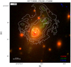 |
Fig. 1. HST composite RGB image of the M1931 BCG: the F160W image is shown in red, the F814W in green, and the F390W in blue. The white contours show to the Hα flux intensity, as measured from MUSE. The cross shows the location of the AGN, as identified according to different diagnostic diagrams; see Sect. 5.5. |
Ehlert et al. (2011) demonstrated that on scales of r ∼ 200 kpc, a spiral of cooler, denser X-ray gas is observed to wrap itself around the core. Such spiral structures arise naturally from mergers and subsequent sloshing. Both the X-ray and optical data reveal oscillatory motion of the cool core along a roughly north-south (NS) direction, as well as extended Intra Cluster Light (ICL), suggesting that the BCG likely experienced a merger within the N-S direction.
Sub-mm ALMA observations (Fogarty et al. 2019) of M1931 have revealed that this BCG harbours one of the largest known reservoirs of cold gas in a cluster core (MH2 = 1.9 ± 0.3 × 10¹⁰ M⊙) as well as large amounts of dust, with several dust clumps having temperatures less than 10 K.
The M1931 BCG represents an example of a cluster with a rapidly cooling core and powerful AGN feedback. The AGN outburst combined with merger-induced motion has most likely led to the cool-core undergoing destruction. This system is probably transitioning between two dominant modes of fuelling for star formation and feedback. It might be evolving from a quasar-mode cooling and feedback typical for higher-redshift cool cores to a weaker and less efficient feedback and cooling mode typical of lower-redshift cluster cores.
3. Data processing
3.1. Observations and data reduction
M1931 was observed in June 2015 with the ESO-VLT MUSE integral field spectrograph (Bacon et al. 2014) under the Guaranteed Time Observations (GTO) programme 095.A-0525 (PI: Kneib, J.-P.). The MUSE pointing consists of three exposures of t = 2924 s each, all centred on the cluster core. Both the raw and reduced data can be found on the ESO Science Archive Facility. We used the raw data and reduced it using the standard calibrations provided by the ESO-MUSE pipeline, version 1.2.1 (Weilbacher et al. 2020). To reduce the sky residuals, we used an additional tool, namely, the Zurich Atmosphere Purge version 1.0 (ZAP, Soto et al. 2016), on the calibrated cubes. This is a tool specially developed for the reduction of IFU data and its core functionality is sky subtraction based on a principal component analysis (PCA). The tool employs filtering and data segmentation to enhance the inherent capabilities of PCA for sky subtraction, it constructs a sky residual spectrum for each spaxel which can then be subtracted from the original data cube and, therefore, it reduces sky emission residuals while preserving the flux and line shapes of the astronomical objects. After accounting for the sky residuals for the three exposures, we combined them using the MUSE Python Data Analysis Framework (MPDAF, Bacon et al. 2016) into a single data cube. The final calibrated data cube has a FoV of 1.1 arcmin2, a spatial sampling of 0.2″ in the wavelength range 4750−9350 Å and a spectral resolution of ∼ 2.5 Å.
The optical IFU data is supplemented by sub-mm ALMA observations from Fogarty et al. (2019), allowing us to link the warm ionised gas to the cold molecular gas component. This sub-mm data set contains Band 3 (beam size: 0.82 arcsec × 0.53 arcsec), Band 6 (beam size: 0.87 arcsec × 0.72 arcsec), and Band 7 (beam size: 0.94 arcsec × 0.78 arcsec) ALMA observations. For the astrometric mismatch correction, we also made use of the CLASH SUBARU and HST photometric data for the M1931 cluster (Postman et al. 2012).
3.2. Astrometric alignment MUSE ALMA
Our analysis of the MUSE and ALMA data requires that the images are aligned to a common astrometric reference frame. For this, we have used the white-light image of the MUSE cube and corrected it for the astrometric mismatch to the SUBARU Suprime-Cam r-band image available from the CLASH project website1, which has excellent alignment with the HST observations. According to Fogarty et al. (2019), the ALMA data is aligned with the HST data and any systematic astrometric alignment errors between the two data sets is not of significant concern. Thus, accounting for the astrometric mismatch between the MUSE image and the Subaru image is equivalent to accounting for the astrometric mismatch between MUSE and ALMA. For the correction of the astrometric mismatch, we developed a PYTHON code using different MPDAF routines. To test the validity of the alignment between the MUSE and SUBARU images, we used an additional PYTHON package – the image registration package – and we measured an offset between the two images, using the Discrete Fourier Transform upsampling methods, of [0.072, −0.17] pixels (i.e. [0.014,−0.034] acrcsec). These values are smaller than one third of the point spread function (PSF) of the MUSE IFS, which is 3.9 pixels; hence, the two images are almost perfectly aligned. To further test the quality of our astrometric correction, we used the coordinates from the Two Micron All-Sky Survey of those stars that fall within the field of view of MUSE and we investigated their positions in our images. We observed a very good agreement with a minimal offset. Moreover, the position we derive for the AGN in the BPT analysis (see Sect. 5.5) from the MUSE data coincides with the location of the sub-mm continuum point source, as observed in the ALMA data.
3.3. MUSE ALMA ratio maps
We created Hα-CO(1-0) and Hα-CO(3-2) flux, velocity, and velocity dispersion ratio (or difference) maps by dividing (or subtracting) the ALMA moment maps from the corresponding MUSE maps. To be able to compare the two data sets, we smoothed the MUSE maps to match the resolution of the ALMA data, using the PYTHON astropy.convolution function. Then we applied the reproject task from the PYTHON astropy package to resample the ALMA data onto the MUSE data pixel grids. This function resamples the data to a new projection using interpolation and it essentially tells the user which pixels in the new image have a corresponding pixel in the old image. Then the re-projected ALMA image was divided (or subtracted) from the MUSE map. It is worth mentioning that due to the lower spectral resolution of the ALMA data, molecular gas kinematics were measured only in the most central regions of the system.
4. Analysis
In the following section, we describe the analysis of the MUSE data, which allows us to study both the gaseous and stellar component of the BCG. Using both the population spectral synthesis code Fitting Analysis using the Differential Evolution Optimisation, (FADO, Gomes & Papaderos 2017) and PORTO3D (Papaderos et al. 2013, Gomes et al. 2016) as well as MPDAF (Bacon et al. 2016), we were able to reliably measure the fluxes of strong emission lines in the optical spectrum, such as [O II] λ3727, Hβ, [O III] λ5007, Hα, [N II] λ6584, and [S II] λ6718, 6732. This, in turn, allowed us to investigate the ionising sources, as well as to derive the electron temperature, electron density, colour-excess, ionisation parameter, star formation rates, (O/H) gas metallicities, and gas kinematics. The star formation history was recovered by employing FADO and PORTO3D. The stellar kinematics were probed using the Galaxy IFU Spectroscopy Tool (GIST, Bittner et al. 2019), which implements the Voronoi binning routine (Cappellari & Copin 2003) and the Python implementation of the Penalized PiXel-Fitting routine (pPXF, Cappellari & Emsellem 2004).
4.1. Emission line flux measurements and star formation history with FADO
From the MUSE data-cube, whose field of view encloses the central regions of the whole M1931 cluster, we extracted a sub-cube centred on the BCG using different MPDAF routines. This sub-cube consists of 90 × 90 spectral pixels (spaxels), which comprises in total 8100 pixels.
Each spaxel of this MUSE sub-cube is fitted with the FADO pipeline (Gomes & Papaderos 2017), which is a tool that is specially designed to perform population spectral synthesis (PSS), with the additional capability of automatically deriving emission line fluxes and equivalent widths (EWs). This tool can be used to identify the star formation history (SFH) that self-consistently reproduces both the observed nebular characteristics of a star-forming galaxy and the stellar spectral energy distribution (SED). Next, FADO is the first PSS (i.e. ‘reverse’) code to employ genetic optimisation under self-consistency boundary conditions. This tool uses an advanced variant of the genetic Differential Evolution Optimization (DEO) algorithm of Storn & Price (1997), which has the advantage of permitting reliable convergence at an affordable expense of computational time. Further improvements of FADO in comparison to other PSS codes include (1) the use of artificial intelligence (AI) concepts for an initial spectroscopic classification and optimisation of the library of simple stellar populations (SSP) spectra; (2) the consideration of nebular emission in spectral fits; and (3) the consistency between the best-fitting SFH and the observed nebular emission characteristics of a star-forming galaxy.
The main modules of FADO are the following: (1) pre-processing of spectral data; (2) spectral synthesis through genetic DEO; and (3) computation and storage of the model output. After the initial guess for the fitting strategy, which depends on the spectral classification and signal-to-noise (S/N) of the input spectra, the SSP library is optimised through AI concepts. There are three fitting strategies: full-consistency (FC) mode, meaning that the spectral modelling aims at consistency between observed and predicted SED continuum and Balmer emission-line luminosities and EWs – this being the default fitting mode of FADO and the one we have used for the fitting. There is also the nebular-continuum mode and the stellar mode. In the fitting module, FADO incorporates various quality checks, such as the auto-determination of the emission-line ratios prior to fitting, an automatic clipping of spurious spectral features, and an examination of the supplied error spectrum. At the first stage, emission-line fluxes and EWs are measured and their quality is investigated. The quality control first involves a sequential check of various quantities and their errors inferred from DEO-based Gaussian line fitting and de-blending, such as the full width at half maximum (FWHM) and the difference between the central wavelength of emission lines. This first step is devised to identify the spurious spectral features (i.e. residuals from cosmics and from sky correction, as well as noise peaks) as outliers and to reject them. In addition, FADO checks whether various emission-line ratios fall within the range of theoretically expected values. This second module also deals with the decision-tree based choices of fitting strategy and convergence schemes, with the computation of predicted Balmer-line luminosities and nebular continuum and with the estimation of the uncertainties. The third FADO module deals with the final measurement of emission-line fluxes and EWs (the widths are not fixed to the same value for all lines, but determined individually) and with the computation of secondary evolutionary quantities, such as light- and mass-weighted stellar age and metallicity.
Before the fitting, all the spaxels were corrected for Galactic foreground extinction with the noao onedspec deredden IRAF routine, using the empirical selective extinction function of Cardelli et al. (1989). For the fitting routine, we have used the library of SSP spectra from Bruzual & Charlot (2003). The SSPs have ages between 1 × 10⁵ and 1 × 10¹⁰ yrs, a resolution of 3 Å across the wavelength range 3200–9500 Å and a wide range of metallicities (1/200, 1/50, 1/5, 1/2.5, 1, and 2.5 Z⊙) for Padova 1994 (Girardi et al. 1996) evolutionary tracks. Also, FADO allows the user to specify which extinction law to be used and we chose the Calzetti law extended to the FUV (Calzetti 2001) for the fitting. It is worth mentioning that the fluxes offered by FADO are corrected for underlying stellar absorption.
The upper panel in Fig. 2 shows the integrated spectrum of the 90 × 90 spaxels MUSE cube, centred on the M1931 BCG in orange, revealing intense nebular emission. The best-fitting synthetic SED is shown in light-blue and it is composed of stellar and nebular continuum emission – the dark green and red spectra, respectively. The five panels from the lower side show the Gaussian fits to the strongest emission lines in the spectrum. These panels allow the user to inspect the quality of the kinematical fitting. The code is designed such as to fit the [O II] as a doublet, even if the lines are completely blended, as in our case. To overcome this problem, we simply added the fluxes offered by FADO for the [O II] emission lines. It is clear from Fig. 2 that the tool manages to properly fit the Hα and [N II] emission lines, which are blended in the spectrum of the M1931 BCG. FADO rejects the Hα + [N II] de-blending solution if the [N II] 6548/6584 lines differ in their FWHM by more than an error-dependent tolerance boundary, defined by the error of the individual line fluxes, or in the case when the redshift-corrected difference between the central wavelength between the Hα and [N II]6548/6584 lines does not match the nominal value. We recovered a median value for the flux errors for log(Hα [N II] λ6584) of ±0.029. It is worth mentioning that the uncertainties in the correction for underlying absorption are included in the errors quoted by FADO for the flux measurements of the emission lines. Therefore, the flux measurements for the blended Hα + [N II] lines can be considered to be robust.
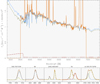 |
Fig. 2. Graphical output of FADO. Upper panel: integrated spectrum of the M1931 BCG orange, as recovered from MUSE. The best-fitting synthetic SED is shown in light-blue, composed of the stellar and nebular continuum emission (dark green and red, respectively). Lower panel: fits to the strongest emission lines, namely, [O II] λ3727, λ3729, Hβ, [O III] λ4959, 5007, Hα, [N II] λ6584, and [S II] λ6718, 6732. |
Additionally, we used the IFU data analysis pipeline Porto3D (Papaderos et al. 2013; Gomes et al. 2016) to double-check emission-line fluxes, EWs, and the SFH, finding an overall good agreement with FADO. While Porto3D uses the PSS code Starlight (Cid Fernandes et al. 2005) for fitting the stellar continuum, it shares with FADO essential aspects in the analysis of the residual nebular emission, the computation of spectral synthesis byproducts (e.g. mass- and light-weighted stellar age, luminosity fraction of stellar populations younger than various age cutoffs) and the storage and graphical output of the results. Additionally, it integrates a rectification technique that suppresses residuals between observed and synthetic stellar SED, this way improving on the extraction and analysis of the nebular component in weak-line sources, such as early-type galaxies (Gomes et al. 2016) and galaxy bulges (Breda & Papaderos 2018).
As a final consistency check, we used MPDAF (Bacon et al. 2016) for the measurements of the emission line fluxes. We developed a PYTHON code performing for each spaxel simultaneous Gaussian line fitting for the emission lines of interest after subtracting the stellar continuum. The fit to each emission line is automatically weighted by the variance of the spectrum. The free parameters of the code are the peak position of the Gaussians, their standard deviation, and the amplitude.
We find a very good agreement between the flux measurements offered by the three different tools, within the errors. Nevertheless, we chose to use the FADO measurements to study the properties of the ionised gas because this tool is aimed at self-consistency between the observed and predicted SED continuum and Balmer emission-line luminosities and EWs. For our analysis, we considered only the spaxels which have an S/N > 10 in the emission line of interest, as well as an S/Nemission line > S/N20 Å blue continuum window and S/Nemission line > S/N20 Å red continuum window. All the emission lines that have an S/N > 10 also have EWs > 10 Å, giving us the confidence that there is a true line detection in the spectrum.
4.2. Determination of the ionising sources
We investigated the ionisation sources in the BCG of M1931 by means of various diagnostic diagrams. Using a set of four strong emission lines, we can reliably distinguish between SF galaxies, Seyfert II galaxies, low-ionisation nuclear emission-line regions (LINERs), and composite galaxies, where gas excitation is powered both by SF regions and an AGN. We used three different diagnostic diagrams on our data set: the classical BPT diagram (Baldwin et al. 1981) as well as the [O III]/Hβ versus [S II]/Hα and the [O III]/Hβ versus [O I]/Hα diagnostic diagram of Veilleux & Osterbrock (1987).
We also tested predictions from different fully radiative shock models calculated with the shock and photoionisation code MAPPINGS V from the Mexican Million Models database of Alarie & Morisset (2019) on the data set to see whether large-scale shocks are responsible for ionising the gas. The database contains models based on previous projects, such as an replica of the Allen et al. (2008) grids including incomplete shock models, an extension of the Allen et al. (2008) grids computed for low metallicities using the abundances of Gutkin et al. (2016), an extension of the Allen et al. (2008) grids computed for different shock ages, and grids for low shock velocities by Delgado-Inglada et al. (2014). All the different grids were tested on M1931 using different metallicities, pre-shock densities, and shock velocities.
In order to more thoroughly investigate the ionising sources in the BCG, we also used the spectral decomposition method of Davies et al. (2017), which is aimed at isolating the contributions of star formation, AGN activity, and LINER emission (in their case, LINER emission is associated to shock excitation, but LINER-like emission can be due to a manifold of mechanisms) to the emission line luminosities of individual spatially resolved regions in galaxies. The method works as follows: from the distribution of the spaxels in the diagnostic diagrams, three ‘basis spectra’ ought to be selected: one representative of pure star formation, one for AGN emission, and one for LINER emission. Then, based on the assumption that the observed luminosity, L, of any emission line, i, in the spectrum of any spaxel, j, from the IFU data cube can be expressed as a linear superposition of the line luminosities of the SF region basis spectrum, the LINER basis spectrum, and the AGN basis spectrum via the following equation:
 (1)
(1)
For each spaxel of the M1931 data cube centred on the BCG, we calculated the superposition coefficients m(j), n(j) and k(j) by performing a least-squares minimisation on Eq. (1), applied to the extinction-corrected fluxes of the four strongest emission lines observed in our spectra, namely [O III] λ5007, Hα, [N II] λ6584, and [S II] λ 6718, 6732. Then we use the computed superposition coefficients to calculate the luminosities of the emission lines of interest associated with star formation, LINER-like excitation, and AGN activity for each spaxel of the data cube. The observed luminosities appear to be well-reproduced by linear superpositions of the line luminosities extracted from the three basis spectra.
However, the selection of the three basis spectra characteristic for SF, AGN, and LINER emission is quite subjective and, simultaneously, the computed model luminosities are highly dependent on their choice. Additionally, these basis spectra, although clearly classifiable as SF, AGN, or LINER, may contain contributions by other gas excitation mechanisms. Therefore, spectral decomposition into these three basis elements may be regarded as a first approximation. For this reason, we have re-calculated the superposition parameters m(j), n(j), and k(j) as well as the model luminosities by performing a second iteration. After the first iteration, we calculated the luminosity of the [O III], Hα, [N II], and [S II] emission lines associated purely with SF for each spaxel of the data-cube. This was done by subtracting from the observed luminosity of each of the aforementioned four emission lines the contribution from the AGN and LINER emission. The median values for the luminosities of the [O III], Hα, [N II], and [S II] emission lines of all spaxels were then used as the new luminosities for the star formation basis spectrum. The emission line luminosities for the AGN and LINER basis spectra were the same ones as in the first iteration. Then we computed the new values for m(j), n(j), and k(j) by conducting least-squares minimisation on Eq. (1) with the new values for Li(SF). The recovered model luminosities are in very good agreement with the observed ones.
4.3. Determination of the electron density and temperature with Pyneb
The electron temperature and density were computed by means of the PyNeb tool (Luridiana et al. 2015), a PYTHON package for analysing emission lines. The main functionality of PyNeb is to solve for line emissivities and to determine electron temperature and density based on observed diagnostic line ratios. The tool works by solving the equilibrium equations for an n-level atom for collisionally excited lines and in the case of recombination lines, it works via interpolation in emissivity tables. Our main interest was the getCrossTemDen function of the tool, a class which cross-converges the temperature and density derived from two sensitive line ratios by inputting the quantity derived with one line ratio into the other and then iterating. When the iteration process ends, the two diagnostics are expected to give self-consistent results. The first line ratio provided by the user must be a temperature-sensitive one and the second a density-sensitive one. A large number of published diagnostic ratios are stored in PyNeb by default, and we tested four of them: ([O III] 4363/5007, [S II]6731/6716), ([N II]5755/6548, [S II] 6731/6716), ([N II] 5755/6584, [S II] 6731/6716), and ([N II] 5755/6584, [Ar IV] 4740/4711). However, it is worth mentioning that we measured very weak [O III] 4363, [Ar IV] 4740, and [Ar IV] 4711 emission for M1931 BCG, indicating that these diagnostics are less robust.
4.4. Determination of the star formation rate and colour excess E(B–V)
The SFR was computed based on the extinction corrected luminosity of the Hα line, both for the integrated spectrum and for each spaxel of the MUSE cube subtending the BCG. The Hα emission line is one of the most reliable SFR indicators, as this nebular emission arises directly from the recombination of HII gas ionised by the most massive O- and early B-type stars, therefore tracing star formation over the lifetimes of these stars. We make the simplifying assumption that the SFR is nearly constant over the past ∼100 Myr and that case B recombination applies and therefore, the Hα luminosity can be used for estimating the SFR following the conversion proposed by Kennicutt (1998a) for solar metallicity and a Salpeter IMF:
 (2)
(2)
However, the intensities of emission lines arising from gas nebulae are affected by selectively absorbing material on the line of sight to the observer. Therefore, the luminosity of the Hα emission line was corrected for extinction based on the Balmer decrement following the equations introduced by Brocklehurst (1971). The colour excess was also calculated based on the Balmer decrement, following the same set of equations. We also computed the SFR surface density as ΣSFR = SFR/area. According to the cosmology, at z = 0.352 the observed scale is 4.9 kpc arcsec−1. As each spatial pixel is 0.2 arcsec, this translates to each pixel having a side of 0.98 kpc.
4.5. Determination of the oxygen abundance and ionisation parameter with HII-CH-mistry
The chemical abundances of galaxies are an important tool for the study of their evolution as they reflect the complex interplay between star formation, gas outflows through winds and supernovae, and galactic gas inflows. The gas-phase oxygen abundances (O/H)s for the M1931 BCG were computed by applying the direct Te based methods described by Pérez-Montero (2017) (Eqs. (38), (40), and (41)), which use, in addition to the emission line flux ratios, the temperature and density of the ionised gas.
As a consistency check, we also used the HII-CH-mistry pipeline (Pérez-Montero et al. 2014) for the computation of the gas phase metallicity. Based on the diagnostic diagrams (see Sect. 5.5), we have seen that the M1931 BCG does not have a strong optical AGN and, therefore, for the computation of (O/H)s, we used HII region grids calculated with Cloudy v.17 (Ferland et al. 2013) using the POPSTAR synthesis evolutionary models for an instantaneous burst with an age of 1 Myr and a Chabrier initial mass function (Chabrier 2003). The grids of the photoionisation models cover a wide range of input conditions of (O/H) and (N/O) abundances and ionisation parameter. The values offered by the code for the (O/H) of each spaxel are in very good agreement (within the errors) with the one obtained by us employing the direct Te methods, giving us the confidence that the measurements are robust. The ionisation parameter was also computed using the HII-CH-mistry tool of Pérez-Montero et al. (2014).
4.6. Determination of the stellar kinematics with GIST
The stellar kinematics were recovered using the Galaxy IFU Spectroscopy Tool (GIST, Bittner et al. 2019), a pipeline written in PYTHON, which extracts stellar kinematics, performs emission-line analysis, and derives stellar population properties from full spectral fitting by exploiting the well-known penalised PiXel-Fitting (pPXF, Cappellari & Emsellem 2004) and Gas and Absorption Line Fitting (GandALF, Sarzi et al. 2006) routines. This pipeline also implements the Voronoi binning (Cappellari & Copin 2003) routine. We used this tool only to recover the stellar kinematics via pPXF. However, it is worth mentioning that the fluxes recovered from GandALF are in good agreement to the ones recovered from FADO, Porto3D, and MPDAF.
To spatially resolve the BCG stellar kinematics, we probed each spaxel of the MUSE data-cube centred on the system, where the S/N of the stellar continuum is higher than 10. The S/N is computed in a 1000 Å window between 5250 Å and 6250 Å, a region of the spectrum that is free of strong emission lines. The S/N of the stellar continuum is so low that we need spatial binning and therefore, we applied the Voronoi tesselation technique. The MUSE cube was tessellated to achieve a S/N of 50 (per bin) in the emission line-free stellar continuum. Therefore, we can measure the velocity fields only in the BCG core, corresponding to a 2 × 2 arcsec region surrounding the supermassive black hole (SMBH). We proceed with a pPXF fit implementing the high resolution, UV-extended ELODIE models of Maraston & Strömbäck (2011). These SSP models are based on the template stellar library ELODIE (Prugniel et al. 2007) merged with the theoretical spectral library UVBLUE (Rodríguez-Merino et al. 2005). The SSPs have a Salpeter initial mass function (Salpeter 1955), a metallicity of Z = 0.02 Z⊙, and ages ranging from 3 Myr to 15 Gyr. The resolution is 0.55 Å (FWHM) and the spectral sampling is 0.2 Å, covering the wavelength range 1000–6800 Å. In order to optimise the pPXF absorption-line fits, all the regions containing strong emission lines in all the spectra were masked, along with the telluric sky-lines at 5577 Å, 5889 Å, 6157 Å, 6300 Å, and 6363 Å. During the pPXF fitting routine, the Hermite coefficients were kept fixed.
5. Results
5.1. Ionised gas flux maps
Figure 3 shows, on the left-hand side, the spatially resolved map of the Hα emission in the M1931 BCG in units of 10−17 ergs s−1 cm−2 for spaxels with an S/NHα > 10. The plot from the right-hand side displays the Hα EW map of the BCG in units Å, for which we have applied the same S/N criterium. The spatial scale in (all) the plots corresponds to 90 by 90 kpc. The galaxies’ intensity peak is coincident with the location of the AGN (as derived according to the different diagnostic diagrams, see Sect. 5.5), and it shows an elongated Hα tail extending ∼30 kpc in the NE direction. The EW peak does not spatially coincide with the emission line brightness peak, but shows more enhanced values in the Hα arm.
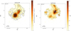 |
Fig. 3. Left: spatially resolved Hα emission line map for the BCG of the M1931 galaxy cluster. The colour-bar shows the flux of the Hα line in units of 10−17 ergs s−1 cm−2. Right: Hα equivalent width map measured in Å. The contours correspond to different levels of flux and EW. The white background in both plots corresponds to spaxels with S/NHα < 10. The cross shows the location of the AGN. |
We observed a similar distribution of fluxes and EWs for [O II] λ3727, Hβ, [O III] λ5007, [N II] λ6584, and [S II] λ 6718, 6732; see Fig. A.1. The similarity between the flux maps of the different emission lines suggests that both recombination and forbidden lines probably originate from the same clouds.
5.2. Comparison between ionised and molecular gas fluxes
We created ratio maps between the line intensities of the ionised and molecular gas (see Fig. 2 from Fogarty et al. 2019), following a normalisation or rescaling by some factor. The left panel of Fig. 4 displays the ratio between the Hα and CO(1-0) flux and the right panel shows the ratio between the Hα and CO(3-2) flux. The Hα to CO flux ratios are close to unity and more or less constant all along the nebula and the peak of the CO flux intensity is located at the same position as the peak of the ionised gas flux intensity. There are some regions that show more enhanced flux for Hα than CO, but there is an overall close similarity between the line intensities of the ionised and molecular gas. The molecular gas is not as extended as the warm ionised gas, but this is likely due to the sensitivity limit or due to the maximum resolution scale of ALMA. The molecular filaments are, thus, co-spatial in projection with the warm ionised gas, which is similar to what has been found in other cool core BCGs (Olivares et al. 2019; Tremblay et al. 2018; Vantyghem et al. 2016).
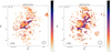 |
Fig. 4. Comparison between Hα and CO linear normalised flux. Left panel: ratio between Hα and CO(1-0) fluxes. Right panel: ratio between the fluxes of Hα and CO(3-2). The cross shows the location of the AGN. The ellipses in the lower right of both panels depict the beam sizes of the ALMA observations. |
5.3. Ionised gas kinematics
The gas kinematics were recovered from the Gaussian fits to the emission lines. We probe each spaxel where S/N > 10 for the emission lines and we compute both the radial velocity and velocity dispersion of the gas from the fits offered by FADO and MPDAF. We observed a very good agreement between the results offered by the two different tools. It is worth mentioning that the kinematics of the [O II] gas were recovered just from the fits offered by MPDAF, making the derived kinematic parameters in this case less robust than for the other emission lines.
The left panel of Fig. 5 displays the Hα radial velocity in km/s, as recovered from FADO. The velocity map is normalised to the BCG’s rest frame, that is, to the velocity obtained from the redshift of the central spaxel (zcenter = 0.3526), whose location is coincident with that of the SMBH. We observed a clear gradient from negative (∼ − 300 km s−1) to positive velocities (∼300 km s−1) relative to the BCGs systemic velocity. We recovered a median value for the error of the velocity of ±30 km s−1. The core of the BCG shows mainly negative gas motions while the gas in the Hα tail shows positive velocities. Such velocity profiles can be indicative of rotation but can also arise from coherently in- or outflowing material with an inclination to the plane of the sky. However, the warm ionised nebula in the innermost 10 kpc of the galaxy is not in dynamical equilibrium, as there are no obvious signs of rotation in the core of the BCG. It is quite a complicated endeavour to firmly establish whether the gas in the tail is inflowing or outflowing from the BCG core. The Hα tail does not seem to have a bi-modal symmetry characteristic of jets and it also does not lie along the axis connecting the cavities observed in the Chandra data by Ehlert et al. (2011). Therefore, the most plausible explanation would be that the redshifted stream of gas in the Hα tail is radially in-falling towards the centre. Such motions of the gas have been observed in many BCGs (e.g. Hamer & Edge 2016, Olivares et al. 2019).
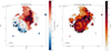 |
Fig. 5. Left: spatially resolved Hα radial velocity map for the BCG of the M1931 galaxy cluster. The colour-bar displays the radial velocity of the Hα gas with respect to the BCG rest frame, measured in [km/s]. Right: spatially resolved Hα velocity dispersion map measured in [km/s]. The white background in both plots corresponds to spaxels with an S/NHα < 10. The cross shows the location of the AGN. The contours show the Hα flux intensity. |
The plot on the right side shows the spatially resolved Hα velocity dispersion map. The measured velocity dispersions in all spaxels were corrected for instrumental broadening. The extended gas has a consistently low velocity dispersion in the order of ∼150 − 250 km s−1, with a median value for the random error of the velocity dispersion of ∼ ± 4 km s−1. The ionised gas shows additional peaks in the line-width, suggesting the gas is more kinematically disturbed in these regions. Dispersions are lowest near the core and increase towards the northern and southern peripheries in the inner-most regions, with the largest dispersions being coincident with the Hα EW peak. The rim with an enhanced dispersion along the north-east-south-west axis lies roughly along the line where the gas velocity changes from negative to positive values. The western side of the Hα tail shows the lowest velocity dispersion. We measured similar radial velocities and velocity dispersions for all other strong emission lines, see Fig. B.1.
5.4. Comparison between ionised and molecular gas kinematics
In the next step, we proceeded to compare the recovered kinematics of the warm ionised gas to those of the cold, molecular gas (Fig. 3 from Fogarty et al. 2019). Figure 6 shows the difference between the ionised and molecular gas kinematics. The panels on the left-hand side display the difference between the systemic velocity of the Hα gas and the velocity of the CO(1-0) gas (top panel) and CO(2-3) gas (bottom panel). The velocity difference maps are predominantly filled with velocity offsets below ±100 km s−1, especially in the core of the BCG, where the velocity differences are in the order of < ± 50 km s−1, indicating that the two gas phases are likely co-moving. The ∼ ± 100 km s−1 velocity differences might be explained by the different spatial resolutions of the MUSE and ALMA data.
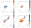 |
Fig. 6. Difference between the kinematics of the ionised gas and those of the cold molecular gas. For a better visualisation, we present the zoomed in plots corresponding to a spatial scale of 45 by 45 kpc. Left side: difference between the radial velocity of the Hα gas and the velocity of the CO(1-0) gas (top) and difference between the velocity of the Hα gas and the velocity of the CO(3-2) gas (bottom). Right side: ratio between the Hα velocity dispersion and the CO(1-0) velocity dispersion (top) and ratio between the velocity dispersion of the Hα gas and the velocity dispersion of the CO(3-2) gas (bottom). The cross in all diagrams shows the location of the AGN, as identified according to the different diagnostic diagrams. The ellipses in the lower right of all panels depict the beam sizes of the ALMA observations. |
The two panels from the right-hand side of Fig. 6 show the ratio maps between the velocity dispersion of the Hα and the CO(1-0) gas on the top side and between the velocity dispersion of the Hα and the CO(3-2) gas on the bottom side. The maps show almost no structure and are close to unity along the nebula. We observe, thus, very good agreement between the dispersions of the warm and cold gas phases, with a median value for the ratio of ∼1.2. It is worth noting that, some structures with more enhanced velocity dispersions for Hα are visible in these maps (ratio ∼3), hinting at the fact that the ionised gas is more kinematically disturbed in these regions than the molecular gas. The velocity dispersion ratio map shows that, on average, the Hα velocity dispersion is by a factor of 1-2 times broader than that for CO(3-2) and CO(1-0). Gaspari et al. (2018) have shown that the warm ionised gas is likely to be more turbulent compared to the cold molecular gas. On the other hand, Tremblay et al. (2018) suggested that lines-of-sight are more likely to intersect larger volumes of warm gas than cold one, which will lead to a broader velocity distribution in the ionised gas than in the molecular component. These two scenarios are, however, hard to distinguish.
To conclude, the comparison between the MUSE and ALMA data reveals evidence that the warm ionised and cold molecular nebulae are to some extent co-spatial and co-moving, consistent with the hypothesis that the optical nebula traces the warm envelopes of molecular clouds. The warm and cold gas are ‘mixed’ in the sense that that pockets of cold (and warm) neutral gas are immersed within the warm ionised gas.
5.5. Ionisation sources
5.5.1. Diagnostic diagrams
Figure 7 shows on the top left hand side the classical BPT diagram (Baldwin et al. 1981), which uses the ratios of [O III]/Hβ vs [N II]/Hα. The blue solid curve represents the theoretical curve of Kewley et al. (2001a,b) and the green dashed one the empirical curve of Kauffmann et al. (2003), which separate SF galaxies from AGNs. The orange solid curve of Schawinski & Thomas (2007) depicts the separation line between Seyfert II galaxies and LINERs. Our results depict a system with mainly composite emission in the BPT, with contribution from both active star formation and an AGN, which is typical for cool-core BCGs (e.g. Loubser & Soechting 2013; Tremblay et al. 2018).
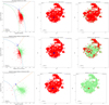 |
Fig. 7. Diagnostic diagrams to distinguish the ionisation mechanism of the nebular gas. First row left: BPT diagram (Baldwin et al. 1981) for all spaxels of the MUSE data cube with S/N > 10 in the emission lines used for the diagnostic. First row middle: BPT distribution on the sky showing the spaxels with Seyfert II emission in blue. First row right: BPT distribution on the sky showing the spaxels which fall in the LINER region of the diagnostic diagram in green. Second row left: diagnostic diagram of Veilleux & Osterbrock (1987) using the [O III]/Hβ vs. [S II]/Hα emission line ratios. Second row middle: distribution on the sky showing the Seyfert II emission in blue. Second row right: distribution on the sky showing the LINER emission in green. Third row left: [O III]/Hβ vs [O I]/Hα diagnostic diagram of Veilleux & Osterbrock (1987). Third row middle: distribution on the sky showing the Seyfert II emission in blue. Third row right: distribution on the sky showing the LINER emission in green. In the latter two diagrams, each data point represents a spaxel of the MUSE cube with an S/N > 10 in each emission line used for the diagnostic. The cross from the upper left corner of all three diagnostic diagrams shows the mean error of the flux measurements. The cross in the neighbouring maps show the location of the AGN. |
The plots from the top middle and top right depict the BPT distribution on the sky, showing the Seyfert II emission in blue and LINER emission in green, respectively. We can identify the location of the SMBH (shown as a cross in all plots), according to the spaxels that fall in the Seyfert II region. It is also clear from these plots that LINER emission can not be associated with the AGN, as this emission is mainly observed in the outskirts of the system.
Figure 7 shows, in the middle-left panel the [O III]/Hβ vs [S II]/Hα and in the lower-left panel, the [O III]/Hβ vs [O I]/Hα diagnostic diagram of Veilleux & Osterbrock (1987). The blue curves in both panels represent the separation curve of Kewley et al. (2001a,b) which divides SF galaxies from AGNs and LINERS. The orange solid curve in both plots depicts the separation curve of Schawinski & Thomas (2007), which differentiates between Seyfert II galaxies and LINERs. The panels from the middle side of both the middle and lower rows show the [S II] and [O I]-BPT distribution on the sky, displaying the Seyfert II emission in blue, while the panels from the right side of both rows display the LINER emission in green. The [O III]/Hβ vs [S II]/Hα diagnostic depicts a system with both HII and LINER emission, while in the [O III]/Hβ vs [O I]/Hα plot, which is a sensitive diagnostic for shocks, the majority of spaxels fall in the LINER region. We also observed considerable variations in the emission line ratio maps used for the computation of the diagnostic diagrams, suggesting that the source of the excitation is not localised to a specific region.
In conclusion, the three diagnostic diagrams reveal mainly composite-LINER emission for the M1931 system, hinting at the fact that there are several mechanisms which ionise the gas. Based on this analysis, we can not draw any definitive conclusions, as the situation for cool-core BCGs is highly complex and likely represents a superposition of several different ionisation sources (e.g. Tremblay et al. 2018; McDonald et al. 2012b).
5.5.2. Fully radiative shock models
Figure 8 shows the fully radiative shock model grids, over-plotted on the three diagnostic diagrams described above. Each black data point represents a spaxel of the MUSE cube with an S/N > 10 in each emission line used for the diagnostic. As can be seen from this plot, the different shock models partially reproduce the measured emission line ratios, mainly for spaxels which fall in the Seyfert II region of the diagnostic diagrams. The only grids which partially seem to fit the data in all three diagnostic diagrams are the ones with a Solar (red lines) and twice Solar (blue lines) metallicity. We observed a similar behaviour for all other shock model grids described in Sect. 4.2 as well.
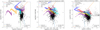 |
Fig. 8. Same as Fig. 7, but showing in addition the predictions from the fully radiative shock models of Allen et al. (2008) computed with MAPPINGS V. We consider a pre-shock density of 1 cm−3, shock velocities ranging from 10 to 350 km s−1, and different metallicities. The choice of these shock velocities are motivated by the observed velocity dispersion of the nebular gas. The red lines depict a grid with solar metallicity, the blue ones a grid with twice solar metallicity, the cyan lines one with metallicities from Dopita et al. (2005), the orange ones a grid with Large Magellanic Cloud metallicities, and the purple ones a grid with Small Magellanic Cloud metallicities. The black data-points represent the spaxels of the MUSE cube, with an S/N > 10 in each emission line used for the diagnostic. The grey data-points represent the spaxels of the MUSE cube, from which we have subtracted the contribution from star formation and AGN emission to the total luminosity of each emission line, after applying the decomposition method of Davies et al. (2017). These data-points are representative for pure LINER-like emission. |
We also accounted for the contribution of star formation, AGN, and LINER-like emission to the luminosity of each emission line in each spaxel of the data cube, allowing us to derive the luminosity of the [O III], [N II], [S II], [O I], Hα, and Hβ gas associated purely with LINER-like emission. The LINER-like emission can arise due to large scale shocks; and if indeed shocks are responsible for ionising the gas in the M1931 BCG, then the fully-radiative shock models should reproduce the pure LINER fluxes of the emission lines in the three diagnostic diagrams.
In Fig. 8, the grey data points represent the spaxels of the MUSE cube, whose luminosities are associated with pure LINER-like emission. Even after removing the contribution from star formation and AGN emission from the luminosity of the emission lines, the different shock grids still do not fully reproduce this modelled emission. Therefore, we concluded that lower velocity shocks seem to play only a minor role as an ionising mechanism in the system. The weakness of the [O III] λ4363 emission also suggests that shocks are not a major ionising mechanism in the M1931 BCG (Voit & Donahue 1997). This is in accordance with the findings of Donahue et al. (2000), who demonstrated, based on HST imaging of cool-core BCGs that, the radio sources in cool-core galaxy clusters are not injecting significant amounts of energy via strong shocks to the emission-line gas and, therefore, shocks cannot be a significant ionising source, nor a source of heating to counterbalance the cooling.
Regarding the AGN emission: we see from the diagnostic diagrams that M1931 does not have a strong optical AGN, as just a few spaxels fall in the Seyfert II region. The weakness of He II λ 4686 Å also rules out such a hard ionising source. Therefore, AGN ionisation seems to influence only the most central regions of the BCG. This is in accordance with the findings of Fogarty et al. (2017), who analysed the impact of AGN emission on the SED fit from the UV through far-IR for M193, and concluded that the effect of AGN emission in M1931 is marginal.
Hence, the dominant source of ionisation in M1931 BCG is a mix between star-formation and other energetic processes which can ‘mimic’ LINER emission. Several hypotheses have been proposed for the source of this extended LINER-like emission. Stellar populations may be responsible for this emission, which could arise due to photoionisation of the gas by young starbursts, or by old pAGB stars (e.g. Shields 1992; Olsson et al. 2010; Loubser & Soechting 2013; Binette et al. 1994; Stasinska et al. 2008). For instance, Byler et al. (2019) studied the predictions of LINER-like emission from pAGB stars, based on fully self-consistent stellar models and photoionisation modelling, and demonstrated, thus, that post-AGB models do indeed produce line ratios in the LINER region of the [S II]/Hα, and [O I]/Hα diagrams and in the ‘composite’ region of the standard BPT diagram. This is exactly what we observe in the diagnostic diagrams for the M1931 BCG. However, these post-AGB star models produce Hα EWs between 0.1 and 2.5 Å, while we observe far higher Hα EWs for M1931 (EWHα > 50 Å throughout the whole nebula; see the right panel of Fig. 3). Therefore, we can rule out post-AGB stars as the dominant source of LINER emission in the M1931 BCG. The LINER-like emission may also be characteristic of starburst-driven outflows (Sharp & Bland-Hawthorn 2010), Lyman continuum photon escape through tenuous warm gas (Papaderos et al. 2013), diffuse ionised gas (DIG) in galactic disks (Zhang et al. 2016), or gas heated by the surrounding medium. The latter mechanism includes photoionisation by cosmic rays, collisional heating by cosmic rays, conduction from hot gas, suprathermal electron heating from the hot gas, X-ray photoionisation, turbulent mixing layers (e.g. Donahue & Voit 1991; Begelman & Fabian 1990; Donahue et al. 2011; McDonald et al. 2012b; Sparks et al. 2012).
Fogarty et al. (2019) also studied the CO excitation mechanisms in the M1931 BCG and their analysis of the CO spectral line energy distribution reveals evidence in support of multiple gas excitation mechanisms in the system, besides star formation. The CO(3-2) transition is highly excited, similar to the cases of quasi-stellar objects (QSOs) and ultraluminous infrared galaxies (ULIRGs), but the CO(4-3) is similar to that observed in normal, star forming galaxies. Therefore, there must be a mechanism that is not related to starbursts which acts as an additional excitation mechanism. The authors conclude that the molecular gas excitation in the BCG is driven by a mix of processes such as SF, radiation from the SMBH, and the interaction between the cold gas and the ICM, in accordance with our findings.
5.5.3. Spectral decomposition method
To test the validity of the spectral decomposition method of Davies et al. (2017), we should check whether the fraction of emission attributed to each ionisation mechanism varies smoothly as a function of the diagnostic line ratios, peaking at the line ratios of the relevant basis spectrum and decreasing as the line ratios become closer to those of the other basis spectra. Figure 9 demonstrates that this is exactly what we observe. The upper three panels depict the BPT diagram while the lower three ones show the diagnostic diagram of Veilleux & Osterbrock (1987), with each data point colour-coded according to the fractional contribution of SF (left), AGN (middle), and LINER (right) to the total Hα emission.
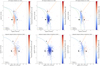 |
Fig. 9. Upper three panels and lower three panels: BPT diagram and the diagnostic diagram of Veilleux & Osterbrock (1987), respectively, with the line ratios extracted from the total emission line fluxes of the individual spaxels. The SF, AGN, and LINER base spectra are depicted as the black square, triangle and circle, respectively. The data points are colour coded according to the fraction of Hα emission attributable to SF (left-hand panels), AGN (middle panels), and ‘LINER’ (right-hand panels), as computed from the spectral decomposition method described in Davies et al. (2017). |
Figure 10 shows the emission line maps for Hα on the upper row, [O III] on the second row, [N II] on the third row, and [S II] on the fourth row colour coded according to the fractional contribution of SF (left), AGN (middle), and LINER-like emission (right) to the total line luminosity.
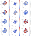 |
Fig. 10. Maps depicting the fractional contribution of SF (left), AGN (middle), ‘LINER’ (right) to the Hα (first row), [O III] λ5007 (second row), [N II] λ6584 (third row) and [S II] (last row) emission lines, as calculated based on the spectral decomposition method. The colour-bar limit displaying the fractional contribution of each ionising mechanism to the total luminosity of the emission lines was set to 0.8, and not the nominal value of 1, for better visualisation purposes. The cross in all diagrams shows the location of the AGN. |
In the maps showing the fractional contribution of SF to the emission line luminosities (first column in Fig. 10), some ‘structures’ become visible, such as the clumps in the vicinity of the AGN (above and to the NW) as well as some clumps in the tail, which are most probably young, SF regions. These regions show in all the emission line maps more enhanced contribution from SF to the total line luminosity, probably making young stars the main ionising mechanism there. These ‘structures’ are coincident with the compact knots seen in the naturally weighted CO(1-0) intensity image, as well as with the UV knots present in HST photometry. In the BCG core at the location coincident with that of the SMBH, the fractional contribution of SF to the total line-luminosity is the smallest. In all the maps showing the AGN contribution to the total line luminosity (second column in Fig. 10), we can observe an enhanced contribution of AGN emission to the total luminosity of the four emission lines in the most central regions of the system, corresponding to the location of the SMBH. In the maps showing the fractional contribution of LINER-like emission to the total line luminosity (third column in Fig. 10), we observe again a low fraction in the central region of the system corresponding to the location of the AGN. A low LINER-like contribution can be found in the star-forming clumps as well.
Possible caveats regarding the spectral decomposition method are related to the fact that the relative luminosities of the emission lines are primarily determined by the relative contributions of different ionisation mechanisms to the line emission, but they are also sensitive to the metallicity and ionisation parameter of the gas.
From the spectral decomposition method, we conclude that the main source of ionisation in the M1931 BCG is a mix between SF and other energetic processes which give rise to LINER-like emission, while AGN ionisation is dominant only in the BCG core. Star formation accounts for ∼50 − 60% of the ionised gas emission, whereas AGN emission accounts only for about ∼10%. The rest of ∼30 − 40% of the energetics needed to excite the gas come from mechanisms which give rise to LINER-like emission. Star formation is, therefore, the main ionising mechanism in the M1931 BCG and the main contribution to the luminosity of the emission lines.
5.6. Electron density and electron temperature
Figure 11 shows, in the upper-left panel, the electron density versus the electron temperature diagnostic diagram for the most central regions of the M1931 BCG. From the M1931 MUSE data cube, we extracted a sub-cube corresponding to the core of the BCG ( circular aperture surrounding the AGN) and one corresponding to the Hα arm and provided the fluxes obtained from the integrated spectra of these two regions to PyNeb. For the core, we obtain degenerate values for the temperature and density when using different line diagnostics. The difference in the ne and Te obtained from different emission lines for the core of M1931 BCG could be due to the superposition of gas components with different physical conditions and gas excitation mechanisms along the line of sight. As we describe in Sect. 5.5, the central region of the BCG is ionised by a mix of processes, and therefore, in this region, we are likely to see the luminosity-weighted average of emission lines arising from different volumes with different physical conditions and, eventually, different kinematics as well. Also, different line ratios are sensitive to different ranges in ne and Te, they therefore are likely to probe different components in the ionised gas.
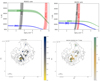 |
Fig. 11. Top-left: electron density vs electron temperature diagnostic diagram for the core of the M1931 BCG. For this plot, we use the following diagnostics: [N II] λ 5755/6548, [N II] λ 5755/6584, [S II] λ 6731/6716, [Ar IV] λ 4740/4711, and [O III] λ 4363/5007. The intersection of the curves gives the best fit electron temperature and density. Top-right: same as top-left, but for the Hα tail of the BCG. Bottom-left: spatially resolved electron temperature map for the BCG of the M1931 cluster. The colour bar shows the temperature measured in [K], as computed using the PyNeb tool, from the [N II] λ5755/6584 emission lines. Bottom-right: electron density map as computed using the PyNeb tool, from the [S II] λ6731/6716 doublet. The colour-bar depicts the density in units of cm−3. The contours in both lower panels show the Hα flux intensity, while the cross shows the location of the AGN. |
The complexity of this issue may already be demonstrated on the example of a relatively ‘simple’ system, such as a blue compact dwarf (BCD) galaxy: James et al. (2009) studied the BCD Mrk 996 based on VLT-VIMOS IFU observations and showed that the ionised gas in the SF nucleus of that galaxy consists of a component with normal density ∼170 cm−3 and broad-line component with an electron density reaching 107 cm−3, which is similar to what we observe in the most central regions of the M1931 BCG.
The plot on the right side of Fig. 11 also displays the electron density versus the electron temperature diagnostic diagram, but for the Hα tail. The different diagnostics offer consistent values for the electron temperature and density, as can be observed from the intersection of the different curves.
The panel from the lower left hand side of Fig. 11 shows the spatially resolved electron temperature map measured in [K], as computed from the [N II] 5755/6584 emission lines for individual spaxels of the M1931 MUSE cube. We measure a median electron temperature of Te ∼ 11230 K and a median random error for the temperature of ∼ ± 220 K. The errors for the electron temperature were calculated with the Bootstrapping method, by assuming that the errors in the line fluxes are Gaussian and adding or subtracting them according to a random key from the measured flux values. These new flux measurements for each spaxel were provided to PyNeb for a new computation of the electron temperature and density. This procedure was repeated a few tens of times to accurately recover the errors for the electron temperature. It is worth mentioning that due to the weakness of the temperature-sensitive emission line [N II] λ5755 we can measure the electron temperature and density only in a small number of spaxels. The spatially resolved electron temperature map shows quite high variations, with the lowest temperatures of about Te ∼ 8000 K in the most central regions of the system. The temperature seems, thus, to decrease towards the core of the BCG. For instance, Vikhlinin et al. (2005) studied the ICM temperature profiles in cluster cores and found that the temperature decreases in the cores of cool-core galaxy clusters, similarly to what we observe for the interstellar medium (ISM) of the BCG.
The panel from the lower-right side of Fig. 11 displays the spatially resolved electron density map in units of cm−3 as computed from the [S II] λ6718, λ6732 emission lines using the PyNeb tool. We measure a median electron density of ne = 361 cm−3, which is a value that is typical for BCGs, with a median error of ∼ ± 60 cm−3 (also computed through the Bootstrapping method). The recovered values for ne are below the critical density threshold of the [S II] doublet, which is ne = 3 × 103 cm−3 (Osterbrock & Ferland 2006), above which the lines become collisionally de-excited. Because of this, we can consider our derivation of the density reliable.
5.7. Color excess E(B–V)
The panel on the left-hand side of Fig. 12 shows the colour excess map for the M1931 BCG. We recovered a median value of E(B − V) = 0.135 and median random error of ±0.002. The error was computed through error propagation by taking only the flux measurement errors and not the calibration uncertainties into account, meaning that the true errors are larger. The highest extinction, in the order of E(B − V)∼0.4 − 0.5 is observed in the BCG core.
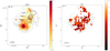 |
Fig. 12. Left: colour excess map for the M1931 BCG as computed from the Balmer decrement. Right: ionisation parameter map, as computed from the HII-CH-mistry tool (Pérez-Montero et al. 2014). The cross in all diagrams shows the location of the AGN. The contours show the Hα flux intensity. The white background corresponds to the spaxels with an S/N < 10 in the emission lines of interest. |
This is in accordance with the findings of Fogarty et al. (2019), who also observed high dust continuum emission in the core of the system, as well as in the Hα tail. The regions 1, 2, and 3, marked by the black ellipses, are the cold dust regions for which Fogarty et al. (2019) measured a temperature of Tdust < 10 K. In the core of the BCG, the dust temperature Tdust, core > 11 K. The dust temperature was estimated based on the continuum emission in ALMA Bands 6 (336.0 GHz) and 7 (468.5 GHz), using the equations introduced by Casey (2012) and a value of β = 1.6 ± 0.38. The ionised gas and dust in the M1931 BCG are more or less co-spatial, except perhaps for region 3, where we measured low emission line fluxes. Intriguingly, the ionised gas EW peak is coincident with the location of the cold dust region 2. The enhanced excitation of the ionised gas in this region can come from collisional excitation of relativistic particles and cold dusty gas (Sparks et al. 2012).
It is worth mentioning that Fogarty et al. (2017) also derived the extinction in the BCG of the M1931 cluster and they obtained a value of A(V) = 0.87 ± 0.21, assuming the Calzetti Law (Calzetti 2001), which corresponds to E(B − V) = 0.21 ± 0.05. Therefore, there is a slight tension between the value inferred by us and that inferred by Fogarty et al. (2017) for the extinction. A possible explanation for the small discrepancy is that the spaxels with > 10σ detections of Hα are systematically less reddened by dust than the broadband filters that Fogarty et al. (2017) used to construct their SED fit from UV through far-IR. However, given the fact that our errors for the colour-excess are underestimated, because they are just the statistical random errors, the two values for E(B − V) can be considered consistent.
5.8. Ionisation parameter
The right panel in Fig. 12 shows the spatially resolved map for the ionisation parameter log(U). This parameter gives the ratio of ionising photon density to hydrogen density and represents a measure of the dimensionless intensity of ionising radiation. We recovered a median value for the ionisation parameter log(U) = −2.9 and a median error of ±0.3. This value for the ionisation parameter is consistent with those observed for star-forming galaxies (e.g. Cresci et al. 2017; Kewley et al. 2019). The highest log(U) values seem to be coincident with the location of the star forming structures, which are visible in Col. 1 of Fig. 10.
5.9. Star formation rates
Figure 13 shows the spatially resolved SFR map for the M1931 BCG in units of M⊙ yr−1. We observe regions with higher SFRs coincident with the BCG core, while in the tail, the SFR levels are lower. From the spaxel by spaxel analysis, we measured a total SFR ∼ 144 M⊙ yr−1 and a random error of ± 0.33 M⊙ yr−1 (computed through error propagation, taking only the flux measurements into account). The recovered SFR surface density is ΣSFR ∼ 147 M⊙ yr−1 kpc−2. However, these values for the SFR and ΣSFR are just the upper limits, because, as we show in Sect. 5.5.3, SF accounts for ∼50 − 60% of the ionised gas emission, while AGN ionisation accounts for about ∼10% and, thus, ∼30 − 40% of the energetics needed to excite the gas come from mechanisms that give rise to LINER-like emission. The Kennicutt (1998a) conversion for the estimation of the SFR was designed for pure star-forming galaxies and, therefore, we should exclude the contribution from AGN and LINER-like emission to the total luminosity of the Hα emission line to accurately estimate the SFR. By doing so, we recover a SFR ∼ 97 M⊙ yr−1 with a random error of ± 0.7 M⊙ yr−1. The integrated star-formation-rate surface density that we recovered, after excluding the contribution of LINER-like and AGN emission to the total line luminosity of Hα, is ΣSFR ∼ 100 M⊙ yr−1 kpc−2. However, LINER-like line ratios could also arise from an over-abundance of O-stars (but not indicating more star formation, Fogarty et al. 2015), meaning that the LINER-like excitation can also partially be due to star formation. Therefore, it might be that the recovered SFR value of ∼ 97 M⊙ yr−1 is slightly underestimated. It is possibly the case that the ‘true’ Hα-based SFR is limited above by a maximum of 144 M⊙ yr−1 and limited below by minimum of 97 M⊙ yr−1.
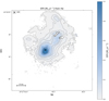 |
Fig. 13. Spatially resolved SFR map calculated from the extinction corrected Hα emission line for each spaxel of the MUSE sub-cube. The colour-bar shows the SFR in units of M⊙ yr−1. The cross shows the location of the AGN, while the contours display the Hα flux intensity. The white background corresponds to the spaxels, which have an S/NHα < 10. |
In comparing to other works, Donahue et al. (2015) reported an unobscured SFR ∼ 90 M⊙ yr−1 for the M1931 BCG from the CLASH HST rest-frame UV data, without accounting for reddening. Ehlert et al. (2011) has reported a SFR ∼ 170 M⊙ yr−1 from broadband Subaru Hα photometry for the same system. Santos et al. (2016) has computed a SFR ∼ 150 ± 15 M⊙ yr−1 from a FIR SED fit using Herschel observations, after removing the AGN contamination. Fogarty et al. (2017) estimated a value for the SFR of ∼ 250 ± 75 M⊙ yr−1 from NUV-FIR SED fitting using photometry from the CLASH HST data set in combination with mid- and far-IR data from Spitzer and Herschel. Fogarty et al. (2015), on the other hand, derived a reddening-corrected value for the UV-continuum estimate of the SFR for the M1931 BCG of 280 ± 20 M⊙ yr−1 using CLASH HST ACS and WFC3 observations. Their derived SFR agrees with the value they obtained in Fogarty et al. (2017) for the SED fit from the UV-FIR. They also estimated the Hα luminosity for the system, for which they derived an SFR of 130 ± 40 M⊙ yr−1. All the Hα based SFR estimates are in accordance with both values derived by us, within the errors. The larger SFR ∼ 250 M⊙ yr−1 values reported by Fogarty et al. (2015, 2017) are heavily influenced by the UV continuum, and possibly reflect the SFR over a longer time period. The lower SFR values are most probably representative for the ongoing star-forming activity.
According to Fogarty et al. (2019), the M1931 BCG has a molecular gas reservoir with a mass of MH2 = 1.9 ± 0.3 × 10¹⁰ M⊙, and together with our inferred SFR, we can calculate the gas depletion time as  , and by doing so, we recover a tdepl ∼ 190 Myr. O’Dea et al. (2008) studied BCGs based on imaging with the Spitzer Space Telescope and inferred a typical gas depletion timescale for such systems of about 1 Gyr. Kennicutt & Evans (2012) demonstrated that when the gas depletion time is shorter the SFR efficiency is higher. This might imply that the M1931 BCG has a high star formation efficiency and that currently, the system is consuming the gas at a higher rate than typical. On the other hand, Voit & Donahue (2011) demonstrated that BCGs with large SFRs (> 10 M⊙ yr−1) have depletion times that are less than 1 Gyr. These depletion times are shorter than those of BCGs with lower SFR levels. The depletion time we infer for the M1931 BCG is thus, not very different from that of other BCGs with large SFRs and it is also similar to that of other star-forming galaxies, especially to those with starburst rates (Díaz-García & Knapen 2020). Hence, the global Kennicutt star formation relation (Kennicutt 1998b) that associates molecular gas quantity with the SFR is not so different in cool-core, multiphase BCGs, and disk galaxies.
In conclusion, the M1931 BCG shows elevated levels of SF in the order of ∼ 97 M⊙ yr−1, with the largest values in the core of the system, which is in accordance with the results of previous studies.
5.10. Oxygen abundances
Figure 14 displays the spatially resolved oxygen abundance map for the BCG of the M1931 cluster. We measured a median gas-phase metallicity 12 + log(O/H) ∼ 8 and an error of ±0.35, with the lowest (O/H) values in the BCG core, and slightly more enhanced values in the outskirts.
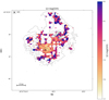 |
Fig. 14. Gas phase metallicity (O/H), as computed by the HII-CH-mistry tool. The colour-bar shows the oxygen abundance in units of 12+log(O/H). The cross shows the location of the AGN, while the contours display the Hα flux intensity. The white background corresponds to the spaxels with an S/N < 10 in the emission lines of interest. |
For instance, Kirkpatrick & McNamara (2015) studied the hot gas-phase metallicity distribution in 29 galaxy cluster cores based on Chandra X-ray data and found that over the life cycle of AGN activity, hot outflows can be responsible for the broadening of abundance peaks in cool-core clusters, and effectively transport metal-enriched gas from the BCG to great distances in the cluster atmospheres. Similarly, Ehlert et al. (2011) studied the ICM metallicity based on Chandra X-ray data in the M1931 cluster and concluded that this cluster core is missing the central metallicity peak which is normally measured in cool core clusters, thus suggesting the bulk transport of hot X-ray gas out to large distances from the centre due to an AGN outburst. This is similar to what we observe for the warm gas in the ISM of this system, with the lowest metallicity values inferred in the core and slightly more enhanced values in the tail. Ehlert et al. (2011) measured a more or less constant ICM metallicity of Z = 0.36 Z⊙ out to distances as large as 400 kpc from the M1931 cluster core, which translates to a 12 + log(O/H) = 8.25. This value is consistent with the gas-phase metallicity we measured in the ISM of the BCG. The similarity may hint at the fact that the gas we observe in the ISM of the galaxy has condensed from the ICM.
5.11. Star formation history
Besides emission line fluxes, EWs, and stellar parameters, FADO can also recover the SFH of a galaxy, ensuring consistency between the best-fitting SFH and the observed nebular emission. As a consistency check, we compared the SFH recovered from FADO to that recovered from Porto3D and we observed a very good agreement between the two.
The SFH module of FADO allows us to recover the stellar mass ever formed within the system:  = 5.9 × 10¹¹ M⊙. This value is in perfect agreement with that inferred by Bellstedt et al. (2016) for the mass of the M1931 BCG using only K-band photometry: M* = 5.9 ± 1.1 × 10¹¹ M⊙. Figure 15 shows the discretised approximation to the best-fitting SFH for the integrated spectrum of the M1931 BCG, as recovered from FADO. The upper panel shows the contribution of the individual SSPs in the best-fitting population vector to the monochromatic luminosity at 6150 Å and the lower one the contribution to the stellar mass as a function of age. It is clear from these two plots that the M1931 BCG had a complex SFH. Approximately 50% of the systems’ stellar mass, that is, M* ∼ 3 × 10¹¹ M⊙, was in place at an early epoch,
  Gyr ago (z ≳ 1.5), followed shortly by subsequent mass build-up episodes, but less strong. This main episode of SF also contributes the most to the luminosity of the galaxy (∼30%). This mass build-up episode is shortly followed by another episode, which occurred 6.3 Gyr ago and leads to the formation of 30% of the mass of the system, that is, to the formation of M* ∼ 1.7 × 10¹¹ M⊙. This second strongest and oldest mass build-up event might be associated with a wet merger (given that there are SSPs of different ages and metallicities contributing to the mass build-up). Hence, most of the mass of the BCG (∼80%) was built up at an early epoch, more than 6 Gyr ago, in accordance with theoretical models, which favour the scenario in which BCG growth follows two–phase hierarchical formation, with rapid cooling and in situ star formation at high redshifts followed by a subsequent growth through repeated mergers, (e.g. De Lucia & Blaizot 2007). Our results are also in accordance with the findings of Collins et al. (2009), who demonstrate that ∼90% of BCGs stellar masses are in place by z = 1. Many other mass build-up events occur for the M1931 BCG over its SFH, but they are less strong than the two initial episodes, and only lead (combined) to the build-up of ∼20% of the mass of the system. The two next-strongest mass build-up events occur at a redshift z ≲ 0.5: one ∼1 Gyr ago – contributing ∼10% to the stellar mass ever formed (leading to a mass build-up of M* ∼ 5.3 × 10¹⁰ M⊙) and ∼13% to the luminosity and the other ∼5.6 × 10⁷ yrs ago – contributing ∼2% to today’s stellar mass (leading to a mass build-up of M* ∼ 1.1 × 10¹⁰ M⊙) and ∼20% to the luminosity. The ages of these two ‘post-assembly’ mass build-up episodes are a good match to the starburst age range that Fogarty et al. (2017) derived for the M1931 BCG using a Bayesian photometry-fitting technique that accounts for both stellar and dust emission from the UV through far-IR. Using a simpler single-burst SFH parameterisation, Fogarty et al. (2017) estimated an age range for a ‘post-assembly’ star formation episode of ∼4.5 × 10⁷ − 2.2 × 10⁸, which is in pretty good agreement with the ages we recover.
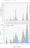 |
Fig. 15. Star formation history of the M1931 BCG. Upper panel: contribution of the individual SSPs in the best-fitting population vector to the monochromatic luminosity at 6150 Å as a function of age. Lower panel: contribution of the SSPs to the total mass of the system as a function of age. The vertical arrow marks the age when 50% of the present-day stellar mass has been in place. The colour coding in both panels display the metallicities of the SSPs, whose values can be found above the upper plot. The vertical bars represent the 1σ uncertainties. The grey vertical lines connecting the two panels mark the ages of the SSPs. The light-blue shaded area in both panels shows an Akima-smoothed (Akima 1970) version of the SSP contributions. |
Other weak mass build-up events probably occurred for the M1931 BCG, leading to the build-up of less than 1% of the stellar mass and less than 10% of the total luminosity of the system. However, robust conclusions of such minor SF episodes are difficult due to the probabilistic nature of PSS. The most recent mass build-up event occurred 1 Myr ago and lead to the formation of 0.2% of the total mass, that is, to the formation of M* = 1.1 × 10⁹ M⊙.
All the weaker episodes of mass build-up, taken at face value, could be attributed to minor dry mergers or to ‘cooling-flow’ induced star formation episodes (or a combination of the two). If we consider all the mass build-up events that happened during the last one Gyr, the redshift of the universe at that time was z ∼ 0.5, an epoch at which wet mergers have mostly ended in galaxy clusters, which are more or less fully assembled. Therefore, the mass build-up episodes which occurred less than 1 Gyr ago can, most probably, not be attributed to wet mergers and associated minor in situ SF episodes, although a contribution from dry mergers cannot be ruled out. For instance, Burke et al. (2015) examined the stellar mass assembly in galaxy cluster cores using CLASH data and found that BCGs grow in stellar mass by a factor of 1.4, on average, from the accretion of their companions and they found major merging to be very rare for their sample. The authors concluded that minor mergers constitute the dominant process for stellar mass assembly of BCGs at low redshifts, but with the majority of the stellar mass from interactions ending up contributing to the ICL rather than building up the system. Similarly, Webb et al. (2015) studied the SFH of BCGs to z = 1.8 from the SPARCS/SWIRE survey and concluded that star formation episodes below z ∼ 1 do not contribute more than 10% to the final total stellar mass of the BCGs and that BCG growth is likely dominated by dry mergers at low z. This is consistent with the recent mass build-up episodes that we infer for the M1931 BCG, which contribute to the build-up of less than 20% of its stellar mass.
Another interpretation could be that these weaker mass build-up events are related to ‘cooling flow’ induced SF episodes, as we know that the M1931 BCG resides in a cool-core cluster. Thermally unstable cooling of the ICM into cold clouds which start sinking towards the SMBH has been shown to explain the ongoing star formation as well as the AGN activity of BCGs (e.g. Voit & Donahue 2015). This scenario is supported by the high SFR levels we measure for the M1931 BCG, which probably cannot be attributed to wet mergers with satellite galaxies, as we know that satellite cluster galaxies approaching the cluster core are expected to be devoid of gas due to ram pressure stripping and starvation. The co-spatiality and kinematics of the ionised and cold gas component, as well as the metallicity of the ISM, also point to a common origin for the two gas-phases, such as cooling from the ICM.
Making a simplified assumption that the SFR was more or less constant for the last 100 Myrs, then a SFR = 97 M⊙ yr−1 yields a stellar mass of ∼1010 M⊙ in this time span (and similarly a SFR = 144 M⊙ yr−1 yields a mass of ∼1.4 × 10¹⁰ M⊙ in the last 100 Myrs). According to Fig. 15, in the last 100 Myrs, ∼3% from of the total mass of the system was formed, yielding a value of about ∼1.7 × 10¹⁰ M⊙. This value is in good agreement to the mass that would have formed in situ in the last 100 Myrs, given the star formation levels inferred from the Hα emission line, leading, thus, to the consideration of SF episodes induced by ‘cooling-flows’ as a good candidate for explaining the recent SFH of the M1931 BCG.
The SFH module of FADO also allows us to put some rough constraints on the stellar parameters, such as the SSP ages (and metallicities). We investigated the stellar age gradients in a region corresponding to the core of the galaxy (i.e.  circular aperture around the SMBH) and in a region encompassing the whole system, and we recovered mainly positive (to flat) age gradients. Stellar ages are lowest in the core of the system and seem to increase towards the outskirts of the galaxy. These findings are also supported by our spatially resolved SFR map, where we demonstrate that the highest SFR levels are confined to the core of the galaxy. Hence, it is expected that the core of the BCG contains a young population of stars. Loubser et al. (2009) demonstrated the youngest BCG cores are mostly line-emitting galaxies in cool-core clusters, similarly to what we observe in the case of the M1931 BCG. Likewise, Edwards et al. (2020) investigated age and metallicity gradients in a sample of 23 low-redshift BCGs (z < 0.7) and observed positive age gradients for six of their systems, and negative gradients for the rest (which is often seen for massive elliptical galaxies). All of the BCGs showing positive age gradients are star forming multi-phase systems, similar to the BCG of the M1931 cluster.
To conclude, both dry mergers or ‘cooling-flow’ induced in situ star formation episodes dominate the mass build-up of M1931 BCGs at late epochs, but they account for only a small fraction of less than 20% of the total mass of the system, while it is likely that in situ star formation (either due to rapid cooling or wet mergers) at early epochs (more than 6 Gyr ago) is what led to the formation of up to ∼80% of the stellar mass of the system.
5.12. Stellar kinematics
Figure 16 shows in the panel on the left-hand side the stellar radial velocity and in the panel on the right hand side the stellar velocity dispersion in the BCG core, as recovered from the GIST pipeline. The stellar velocity map is normalised to the BCGs’ rest frame, that is, to the velocity of the central bin, whose position is coincident with that of the SMBH. The recovered stellar velocity dispersions are corrected for instrumental broadening. While the stellar radial velocity shows a gradient from −200 to 200 km s−1 (with a median error for the radial velocity of ±12 km s−1) with respect to the systemic velocity of the BCG, being indicative of rotation, the values for the stellar velocity dispersion are far higher, ranging from 300 km s−1 up to ∼650 km s−1 (with a median error for the velocity dispersion of ±12 km s−1). This means that the BCG core is dispersion dominated, that is, a slow rotator, which is expected for massive, elliptical galaxies. Since this high-stellar-velocity dispersion is going to be preserved after the gas was consumed by SF or ejected by the AGN, our data shows an intermediate-late stage in the assembly history of present-day massive early-type galaxies (or central dominant galaxies) at the centre of galaxy clusters.
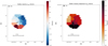 |
Fig. 16. Left: radial velocity of the stars with respect to the systemic velocity of the most central region of the system. Right: velocity dispersion of the stars in the BCG. The colour-bar in both plots depicts the radial velocity and velocity dispersion in units of [km/s]. Due to the low S/N in the stellar continuum, the data needs binning, and we can, therefore, measure the stellar kinematics only in the core of the system. To better visualise the results, we present maps showing just the most central regions of the BCG, corresponding to a spatial scale of 45 × 45 kpc. The white background corresponds to the spaxels, where the S/Nstellar continuum < 10. The cross shows the location of the AGN. |
5.13. Comparison stellar and gaseous kinematics
Figure 17 displays the difference between the systemic velocity of the stars and the Hα gas on the left-hand side and on the right-hand side, the ratio between the velocity dispersions of the stellar and ionised gaseous component. For this comparison, we use the stellar kinematics recovered by the GIST pipeline for the un-binned data. We measure velocity differences between the stellar and gaseous component as high as ∼ ± 200 km s−1, and a median value for the ratio between the velocity dispersion of stars and gas of 2.4. Hence, the stars have much higher velocity dispersions than the gas.
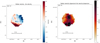 |
Fig. 17. Left: difference between the radial velocities of the stars and the Hα gas in the BCG core. Right: ratio between the velocity dispersion of the stars and the Hα gas in the core of the system. To better visualise the results, we present maps showing just the most central regions of the BCG, corresponding to a spatial scale of 45 × 45 kpc. The white background corresponds to the spaxels, where the S/Nstellar continuum < 10. The cross shows the location of the AGN. |
The gaseous and stellar kinematics in the M1931 BCG core are, thus, decoupled, with the gaseous component not following the potential well of the stars. Such decoupled kinematics have been observed in other BCGs (e.g. Hamer & Edge 2016; Loubser & Soechting 2013). The kinematics of the gas are more closely related to the turbulence and bulk motions in the hot ICM than they are related to the motions of the stars. The high velocity dispersion of the stars argues strongly that the gas has originated from the more quiescent circumgalactic medium, and not from the stars themselves. These findings are in accordance with the predictions of the precipitation model (Voit et al. 2017) as well as of those of the chaotic cold accretion model (Gaspari et al. 2018), both of which state that the gas motions track the much larger X-ray gas reservoir rather than the stellar component. The precipitation models also predict that σgas < 0.5 ⋅ σstars, in accordance with what we observe for the M1931 BCG.
6. Discussion
The archival MUSE and ALMA observations used in our analysis of the M1931 BCG reveal an extended, filamentary system that displays dynamically unrelaxed structures with disturbed motions along the filaments. Both the molecular and ionised gas distribution shows a nuclear emission component closely related to the BCGs’ core, as well as a set of clumpy filaments, which form an elongated Hα arm, extending ∼30 kpc in the NE direction. Both gas phases are co-spatial and co-moving, with the molecular gas being spatially distributed along the brightest emission from the warm ionised nebula.
These findings are in accordance with the hypothesis that the optical nebula traces the envelopes of the cold molecular clouds. As we have seen in Sect. 5.5, the cloud surfaces are excited by a broad range of mechanisms and they are bright in Balmer and forbidden line emission. The pockets of cold gas are immersed within ionised gas, and the in situ SF within the molecular clouds as well as interactions with the ICM are the most plausible mechanisms that give rise to extended Hα emission all over the core and the NE filament.
Such correlations between the two gas phases can be interpreted as the manifestation of a common origin, like the condensation of low-entropy ICM gas through thermal instabilities. The ICM surrounding the Hα tail has the lowest entropy according to Ehlert et al. (2011), therefore, being a prime candidate for the reservoir of gas that cools to become star-forming molecular gas. Moreover, the recovered values for the gas phase metallicity in the BCG are consistent with those recovered by Ehlert et al. (2011) for the ICM, within the acceptable errors. These findings support the scenario, that the warm gas has condensed from the ICM, without being further polluted by the stars in the system.
For instance, Fogarty et al. (2017) studied the nature of feedback mechanisms in the 11 CLASH BCGs and their results strongly suggest that thermally unstable ICM plasma with a low cooling time is the source of material that forms the reservoir of cool gas fuelling star formation in the BCGs and that BCG star formation and feedback either exhausts the supply of this material on gigayear timescales or settles into a state with relatively modest and continuous star formation.
The role of AGN feedback on the turbulent and chaotic behaviour of the gas was emphasised by Voit et al. (2017) who demonstrated that the AGN jets and bubbles can promote condensation of the hot ambient medium by raising some of it to greater altitudes and thus lowering its (tcool/tff) ratio. After the condensates form, they start raining down towards the SMBH, representing additional fuel for both star formation and AGN activity. In simulations, complex arcs of gas fall back into the centres of BCGs after initially being propelled outwards by AGN jets and cavities (Gaspari et al. 2013; Li et al. 2015), similar to what we observe in the M1931 BCG. The significance of uplift and radial infall is now an integral aspect of the precipitation model (Voit & Donahue 2015; Voit et al. 2017) as well as of the chaotic cold accretion model (Gaspari et al. 2018; Tremblay et al. 2018).
The kinematics of the gas in the M1931 BCG point out to such a scenario. According to Fogarty et al. (2019) and to our observations, the molecular gas in the Hα tail is probably falling inward at ∼300 km s−1, with the ionised gas component closely following these motions, as can be seen from the left panel of Fig. 5. The redshifted stream of gas we observe would, thus, relate to the material that is radially in-falling towards the centre of the system. These infalling clouds can provide a substantial component of the mass flux toward the SMBH accretion reservoir, while the physical conditions of the gas within these clouds could satisfy the criteria for the ignition of star formation.
Moreover, the gaseous and stellar kinematics are decoupled, as they do not share a common velocity field, with the stars showing larger velocities than the gas. These distinct properties of the gas velocities and the stars’ velocities suggest that the motion of the gas is more closely related to the turbulence and bulk motions within the ICM than it is related to the motion of the stars in the system.
The kinematics of the warm and cold gas phases lead us to conclude that the AGN in the system might have recently experienced an energetic outburst. This AGN outburst temporarily led to the condensation of the uplifted gas, which is now probably cycling back down towards the AGN, promoting an elevated star formation rate of ∼ 100 M⊙ yr−1. The observed distribution of dust in the system (Fogarty et al. 2019) points to an uplift mechanism, with dust emission most prominent in the core and at the furthest extremity of the tail. The observed distribution of the gas phase metallicity can also hint to such an uplift mechanism. We observe the lowest (O/H) values of ∼ 7.9 in the most central regions of the systems, while in the Hα tail, the metallicity is slightly higher. This might mean that the metal enriched gas has been expelled outwards from the centre due to AGN outflows.
However, the infalling multiphase tail is not aligned with the jet axis. This is implied by features that are consistent with E − W oriented X-ray cavities observed in the Chandra data (Ehlert et al. 2011). This indicates that the gaseous component either might have originally formed at the interface between the jet-inflated cavities and the ICM and then migrated away from these positions; or it might have formed at an earlier epoch, sufficiently long ago for the X-ray cavities to have dissipated (Fogarty et al. 2019).
The cloud envelopes in this system are ionised by a superposition of many physical processes, including photoionisation from young stars and other mechanisms that give rise to LINER-like emission, the best candidates being photoionisation by cosmic rays, conduction from the hot ICM, X-ray photoionisation, turbulent mixing layers, or collisional heating. In terms of the AGN emission, it dominates only in the BCG core; see Figs. 7 and 10. This is in accordance with the findings of Fogarty et al. (2019), whose analysis of the CO spectral line energy distribution in the M1931 BCG also reveals evidence for multiple gas excitation mechanisms including SF and the interaction between the molecular gas and the ICM and AGN emission. According to Donahue et al. (2011), such multiphase-star forming BCGs also tend to have unusually luminous vibrational and rotational H2 lines, which are by far more luminous than in normal, star-formation objects. The emission in such galaxies is not fit by H2 gas at a single excitation temperature, hinting to the fact that there must be a mix of excitation mechanisms at play, in accordance with our findings. The spectral decomposition method of Davies et al. (2017) allows us to infer the fractional contribution of each mechanism to the total luminosity of the emission lines. Ionisation from star formation has a fractional contribution to the luminosity of the emission lines of about 50–60%, whereas AGN emission accounts only for ∼10%. LINER-like emission accounts for 30–40% of the energetics needed to ionise the gas. The occurrence of such ‘composite’ emission is typical for cool-core BCG. For example, Tremblay et al. (2018), Iani et al. (2019), Hamer & Edge (2016) also studied (cool-core) BCGs based on IFU data and infer composite emission for their systems in the BPT diagram and concluded that the systems are ionised by a superposition of many physical processes.
The spectral decomposition method also allows us to recover a more accurate estimate for the SFRs, after excluding the fractional contribution of AGN and LINER emission to the luminosity of the Hα line, inferring a lower limit of SFR ∼ 97 M⊙ yr−1. This value for the SFR, as well as the one we inferred without removing the contribution from both AGN and LINER to the luminosity of the Hα line, i.e. the SFR value of ∼ 144 M⊙ yr−1, are in accordance with literature Hα based SFRs for the M1931 BCG, within the errors (Ehlert et al. 2011; Donahue et al. 2015; Fogarty et al. 2015, 2017).
The properties of the ionised gas that we infer by analysing the spectrum of each spectral pixel of the MUSE cube, such as the electron temperature, density, colour excess, and the ionisation parameter, are typical for star forming systems. We also computed the physical properties of integrated regions in the system; see Appendix C for more details.
The temperature that we infer from the [N II] 5755/6584 emission lines is on the order of Te = 11 000 K, with the lowest values observed in the most central regions of the system. These values are in accordance with the ones inferred for the BCG of the cool-core cluster Abell 2597 by Voit & Donahue (1997).
For instance, Hamer & Edge (2016) and Iani et al. (2019) determined the electron density for their sample of BCGs based on the [S II] 6731/6716 emission line ratio and their inferred values, on the order of a few hundred cm−3, are in very good agreement with the value of ne = 361 cm−3 that we determine for the M1931 BCG.
We observe the highest density and extinction (E(B − V)∼0.5) in the most central regions of the system, in accordance with the findings of Fogarty et al. (2019), who also measures the highest dust continuum emission in the core of the system. Thus, the densest, and perhaps dustiest gas is found to be coincident (and to the South) with the nucleus, where the radio source is also detected.
The measured ionisation parameter is in the order of log(U) = −2.9, a value that is typical for star-forming galaxies according to Kewley et al. (2019), and it shows some variation within the nebula, hinting at the fact that the source of excitation is not confined to a specific region.
To conclude, it is possible that the molecular gas and ionised nebula at the centre of the M1931 cluster is a galaxy-scale ‘fountain’ that is similar to what was observed by Tremblay et al. (2018) and Olivares et al. (2019) for their sample of BCGs: the AGN feedback uplifted the low- entropy gas, which ultimately condensed and began raining back toward the galaxy centre from which it came. This rain of gas back to the SMBH accretion reservoir continues to promote SF and further AGN feedback, in accordance with the theoretical predictions of the chaotic cold accretion model (Gaspari et al. 2018). However, these ‘cooling-flow’ induced SF-episodes, in combination with dry mergers, lead to the build-up of less than 20% of the current day stellar mass of the BCG.
7. Conclusions
Based on VLT-MUSE optical integral field spectroscopy, here we investigate the BCG of the massive cool-core CLASH cluster MACS 1931.8-2635, at a redshift of z = 0.35, in terms of its spatially resolved star formation activity, ionisation sources, chemical abundances, and gas and stellar kinematics. The optical MUSE IFS data is supplemented by sub-mm ALMA observations, allowing us to link the properties of the warm ionised gas to those of the cold molecular gas component. Employing different tools on the optical data, we were able to reliably measure: (1) the fluxes of strong emission lines, which allow us to quantitatively determine the physical conditions of the warm ionised gas; (2) the SFH; and (3) the kinematics of the stellar component.
The principal findings of our analysis can be summarised as follows:
-
The ionised and molecular gas components are co-spatial. The normalised Hα to CO flux ratios are close to unity along the nebula and the peak of the CO flux intensity is located at the same position as the peak of the ionised gas flux intensity.
-
The ionised and molecular gas components are co-moving. We measure a gradient from ∼ − 300 to ∼300 km s−1 with respect to the BCG rest-frame and consistently low velocity dispersions in the order of ∼150 − 250 km s−1 for the ionised gas. The diffuse gas confined into the tail is likely falling inward, providing additional fuel for SF and AGN feedback, in accordance with models of chaotic cold accretion.
-
The main source of ionisation in the M1931 BCG is a mix between star formation and other energetic processes which give rise to LINER-like emission, the main candidates being heating of the gas by the surrounding medium and not ionisation by pAGB stars. The AGN ionisation only dominates in the BCG core.
-
After applying the spectral decomposition method, we recover an SFR of ∼ 97 M⊙ yr−1, with the most elevated levels in the BCG core. However, star formation accounts only to ∼50–60% of the energetics that is required to ionise the warm gas. AGN emission accounts for ∼10% of the ionised gas emission, while the rest of ∼30 − 40% of the energetics needed to excite the gas come from mechanisms that give rise to LINER-like emission. Star formation is, thus, the main contribution to the Hα flux.
-
The median values recovered from the spatially resolved maps for the electron density, electron temperature, extinction, and ionisation parameters are typical for star-forming systems and in good agreement with other studies of cool-core BCGs.
-
We measure a median value for the gas phase metallicity of 12 + log(O/H) ∼ 8 ± 0.35, with the lowest values observed in the BCG core. Ehlert et al. (2011) measure an ICM metallicity of 12 + log(O/H) = 8.25, a value that is consistent with the gas-phase metallicity we measure in the ISM of the BCG. This may hint at the fact that the warm gas we observe in the ISM of the galaxy has condensed from the ICM.
-
About 80% of the systems stellar mass formed more than 6 Gyr ago (i.e. at z ≳ 1.5), followed by subsequent but weaker mass build-up episodes. The SFH of the M1931 BCG is in accordance with theoretical models that suggest a two phase hierarchical formation for BCGs: in situ SF at high-z followed by subsequent mass growth through dry mergers or ‘cooling-flow’ induced SF episodes. Both dry mergers or in situ SF generated by ICM cooling account for less than 20% of the stellar mass of the M1931 system within the last 1 Gyr (i.e. at z ≲ 0.5).
-
The stellar kinematics reveal a dispersion dominated system, which is typical for massive elliptical galaxies.
-
The gas motions are decoupled from the stellar kinematics and are more closely related to the bulk motions of the ICM. The velocity dispersion of the gaseous component is approximately two times lower than the velocity dispersion of the stellar component, in accordance with the predictions of the precipitation model.
Most of the Python codes and Jupyter Notebooks that we have developed for this analysis are publicly available in an online GitHub repository (Ciocan2021-MACS1931-BCG-codes)2.
This code repository is archived at DOI: 10.5281/zenodo.4458242, and also available at https://github.com/ciocanbianca/Ciocan2021_MACS1931_BCG_codes
Acknowledgments
We would like to express our deep gratitude to the members of the observational extragalactic astrophysics group from the department of astrophysics, University of Vienna. Special thanks to Christian Maier and Asmus Böhm for all the valuable discussions and pieces of advice! We would also like to express our gratitude to Maria Luísa Gomes Buzzo for all her help related to analysis of the MUSE data. We would especially like to thank the anonymous referee for providing constructive comments and help in improving the manuscript. This work was supported through FCT grants UID/FIS/04434/2019, UIDB/04434/2020, UIDP/04434/2020 and the project “Identifying the Earliest Supermassive Black Holes with ALMA (IdEaS with ALMA)” (PTDC/FIS-AST/29245/2017). This research made use of the following PYTHON packages: Astropy (Astropy Collaboration 2013), numpy (van der Walt et al. 2011), matplotlib (Hunter 2007), MPDAF (Bacon et al. 2016), CMasher (van der Velden 2020).
References
- Akima, H. 1970, J. ACM (JACM), 17, 589 [Google Scholar]
- Alarie, A., & Morisset, C. 2019, RMxAA, 55, 377 [Google Scholar]
- Allen, M. G., Groves, B. A., & Dopita, M. 2008, ApJS, 178, 20 [Google Scholar]
- Astropy Collaboration (Robitaille, T. P., et al.) 2013, A&A, 558, A33 [NASA ADS] [CrossRef] [EDP Sciences] [Google Scholar]
- Bacon, R., Vernet, J., Borisova, E., et al. 2014, MSNGR, 157, 13 [Google Scholar]
- Bacon, R., Piqueras, L., Conseil, S., et al. 2016, Astrophysics Source Code Library [record ascl:1611.003] [Google Scholar]
- Baldwin, J. A., Phillips, M. M., & Terlevich, R. 1981, PASP, 93, 5 [NASA ADS] [CrossRef] [EDP Sciences] [Google Scholar]
- Begelman, M. C., & Fabian, A. C. 1990, MNRAS, 244, 26 [Google Scholar]
- Bellstedt, S., Lidman, C., Muzzin, A., et al. 2016, MNRAS, 460, 2862 [NASA ADS] [CrossRef] [Google Scholar]
- Binette, L., Magris, C. G., Stasinska, G., et al. 1994, A&A, 292, 13 [Google Scholar]
- Bittner, A., Falcón-Barroso, J., Mendez-Abreu, J., et al. 2019, A&A, 628, A117 [NASA ADS] [CrossRef] [EDP Sciences] [Google Scholar]
- Breda, I., & Papaderos, P. 2018, A&A, 614, A48 [NASA ADS] [CrossRef] [EDP Sciences] [Google Scholar]
- Brocklehurst, M. 1971, MNRAS, 153, 471 [NASA ADS] [CrossRef] [Google Scholar]
- Bruzual, G., & Charlot, S. 2003, MNRAS, 344, 1000 [NASA ADS] [CrossRef] [Google Scholar]
- Burke, C., & Collins, C. 2013, MNRAS, 434, 2856 [NASA ADS] [CrossRef] [Google Scholar]
- Burke, C., Hilton, M., & Collins, C. 2015, MNRAS, 449, 2353 [NASA ADS] [CrossRef] [Google Scholar]
- Byler, N., Dalcanton, J., Conroy, C., et al. 2019, AJ, 158, 2 [NASA ADS] [CrossRef] [Google Scholar]
- Calzetti, D. 2001, PASP, 113, 1449 [NASA ADS] [CrossRef] [Google Scholar]
- Cappellari, M., & Copin, Y. 2003, MNRAS, 342, 345 [NASA ADS] [CrossRef] [Google Scholar]
- Cappellari, M., & Emsellem, E. 2004, PASP, 116, 138 [NASA ADS] [CrossRef] [Google Scholar]
- Cardelli, J. A., Clayton, G. C., & Mathis, J. S. 1989, ApJ, 345, 245 [NASA ADS] [CrossRef] [Google Scholar]
- Casey, C. M. 2012, MNRAS, 425, 3094 [Google Scholar]
- Cerulo, P., Orellana, G. A., & Covone, G. 2019, MNRAS, 487, 3759 [Google Scholar]
- Chabrier, G. 2003, PASP, 115, 763 [Google Scholar]
- Cid Fernandes, R., Mateus, A., & Sodré, L. 2005, MNRAS, 358, 363 [NASA ADS] [CrossRef] [Google Scholar]
- Collins, C. A., Stott, J. P., Hilton, M., et al. 2009, Nature, 458, 603 [NASA ADS] [CrossRef] [PubMed] [Google Scholar]
- Cresci, G., Vanzi, L., Telles, E., et al. 2017, A&A, 604, A101 [NASA ADS] [CrossRef] [EDP Sciences] [Google Scholar]
- Davies, R. L., Groves, B., Kewley, L., et al. 2017, MNRAS, 470, 4974 [NASA ADS] [CrossRef] [Google Scholar]
- Delgado-Inglada, G., Morisset, C., & Stasińska, G. 2014, MNRAS, 440, 536 [NASA ADS] [CrossRef] [Google Scholar]
- De Lucia, G., & Blaizot, J. 2007, MNRAS, 375, 2 [NASA ADS] [CrossRef] [Google Scholar]
- Díaz-García, S., & Knapen, J. H. 2020, A&A, 635, A197 [CrossRef] [EDP Sciences] [Google Scholar]
- Donahue, M., & Voit, G. M. 1991, ApJ, 381, 361 [Google Scholar]
- Donahue, M., Mack, J., Voit, G. M., et al. 2000, ApJ, 545, 670 [NASA ADS] [CrossRef] [Google Scholar]
- Donahue, M., Bruch, S., Wang, E., et al. 2010, ApJ, 715, 881 [NASA ADS] [CrossRef] [Google Scholar]
- Donahue, M., de Messiéres, G. E., O’Connell, R. W., et al. 2011, ApJ, 732, 40 [NASA ADS] [CrossRef] [Google Scholar]
- Donahue, M., Connor, T., Fogarty, K., et al. 2015, ApJ, 805, 177 [NASA ADS] [CrossRef] [Google Scholar]
- Dopita, M. A., Groves, B. A., Fischera, J., et al. 2005, ApJ, 619, 755 [NASA ADS] [CrossRef] [Google Scholar]
- Edwards, L. O. V., Salinas, M., Stanley, S., et al. 2020, MNRAS, 491, 2617 [CrossRef] [Google Scholar]
- Ehlert, S., Allen, S. W., Von Der Linden, A., et al. 2011, MNRAS, 411, 1641 [NASA ADS] [CrossRef] [Google Scholar]
- Fabian, A. C., & Nulsen, P. E. J. 1977, MNRAS, 180, 479 [NASA ADS] [CrossRef] [Google Scholar]
- Ferland, G. J., Porter, R. L., van Hoof, P. A. M., et al. 2013, Rev. Mex. Astron. Astrofis., 49, 137 [Google Scholar]
- Fogarty, K., Postman, M., Connor, T., et al. 2015, ApJ, 813, 117 [CrossRef] [Google Scholar]
- Fogarty, K., Postman, M., Larson, R., et al. 2017, ApJ, 846, 103 [NASA ADS] [CrossRef] [Google Scholar]
- Fogarty, K., Postman, M., Li, Y., et al. 2019, ApJ, 879, 103 [Google Scholar]
- Gaspari, M., Ruszkowski, M., & Oh, S. P. 2013, MNRAS, 432, 3401 [NASA ADS] [CrossRef] [Google Scholar]
- Gaspari, M., McDonald, M., Hamer, S. L., et al. 2018, ApJ, 854, 167 [NASA ADS] [CrossRef] [Google Scholar]
- Gomes, J. M., Papaderos, P., Kehrig, C., Vílchez, J. M., & Lehnert, M. D. 2016, A&A, 588, A68 [NASA ADS] [CrossRef] [EDP Sciences] [Google Scholar]
- Gomes, J. M., & Papaderos, P. 2017, A&A, 603, A63 [NASA ADS] [CrossRef] [EDP Sciences] [Google Scholar]
- Girardi, L., Bressan, A., Chiosi, C., Bertelli, G., & Nasi, E. 1996, A&AS, 117, 113 [NASA ADS] [CrossRef] [EDP Sciences] [Google Scholar]
- Gutkin, J., Charlot, S., & Bruzual, G. 2016, MNRAS, 462, 1757 [NASA ADS] [CrossRef] [Google Scholar]
- Hamer, S. L., Edge, A. C., et al. 2016, MNRAS, 460, 1789 [Google Scholar]
- Hunter, J. D. 2007, Comput. Sci. Eng., 9, 90 [NASA ADS] [CrossRef] [Google Scholar]
- Iani, E., Rodighiero, G., Fritz, J., Cresci, G., et al. 2019, MNRAS, 487, 5593 [Google Scholar]
- James, B. L., Tsamis, Y. G., Barlow, M. J., et al. 2009, MNRAS, 398, 2 [NASA ADS] [CrossRef] [Google Scholar]
- Kauffmann, G., Heckman, T. M., Tremonti, C., et al. 2003, MNRAS, 346, 1055 [Google Scholar]
- Kennicutt, Jr., R. C. 1998a, ARA&A, 36, 189 [Google Scholar]
- Kennicutt, Jr., R. C. 1998b, ApJ, 498, 541 [NASA ADS] [CrossRef] [Google Scholar]
- Kennicutt, R. C., & Evans, N. J. 2012, ARA&A, 50, 531 [NASA ADS] [CrossRef] [Google Scholar]
- Kewley, L. J., Heisler, C. A., Dopita, M. A., et al. 2001a, ApJS, 132, 37 [NASA ADS] [CrossRef] [Google Scholar]
- Kewley, L. J., Dopita, M. A., Sutherland, R. S., et al. 2001b, ApJ, 556, 121 [NASA ADS] [CrossRef] [Google Scholar]
- Kewley, L. J., Nicholls, D. C., Sutherland, R. S., et al. 2019, ARA&A, 57, 511 [Google Scholar]
- Kirkpatrick, C. C., & McNamara, B. R. 2015, MNRAS, 452, 4361 [NASA ADS] [CrossRef] [Google Scholar]
- Lavoie, S., Willis, J. P., Democles, J., et al. 2016, MNRAS, 462, 4141 [NASA ADS] [CrossRef] [Google Scholar]
- Li, Y., & Bryan, G. L. 2014, ApJ, 789, 153 [NASA ADS] [CrossRef] [Google Scholar]
- Li, Y., Bryan, G. L., Ruszkowski, M., et al. 2015, ApJ, 811, 73 [NASA ADS] [CrossRef] [Google Scholar]
- Li, Y., Ruszkowski, M., & Bryan, G. L. 2017, ApJ, 847, 106 [NASA ADS] [CrossRef] [Google Scholar]
- Lauer, T. R., Postman, M., Strauss, M. A., et al. 2014, ApJ, 797, 82 [Google Scholar]
- Loubser, S. I., & Soechting, I. K. 2013, MNRAS, 431, 2933 [Google Scholar]
- Loubser, S. I., Sánchez-Blázquez, P., Sansom, A. E., & Soechting, I. K. 2009, MNRAS, 398, 133 [NASA ADS] [CrossRef] [Google Scholar]
- Luridiana, V., Morisset, C., & Shaw, R. A. 2015, A&A, 573, A42 [NASA ADS] [CrossRef] [EDP Sciences] [Google Scholar]
- Maraston, C., & Strömbäck, G. 2011, MNRAS, 418, 2785 [NASA ADS] [CrossRef] [Google Scholar]
- McDonald, M., Bayliss, M., Benson, B. A., et al. 2012a, Nature, 488, 349 [NASA ADS] [CrossRef] [Google Scholar]
- McDonald, M., Veilleux, S., & Rupke, D. S. N. 2012b, ApJ, 746, 153 [NASA ADS] [CrossRef] [Google Scholar]
- McNamara, B. R., & Nulsen, P. E. J. 2007, ARA&A, 45, 117 [NASA ADS] [CrossRef] [MathSciNet] [Google Scholar]
- McNamara, B. R., Russell, H. R., Nulsen, P. E. J., et al. 2014, ApJ, 785, 44 [NASA ADS] [CrossRef] [Google Scholar]
- Merten, J., Meneghetti, M., Postman, M., et al. 2015, ApJ, 806, 4 [Google Scholar]
- O’Dea, C. P., Baum, S. A., Privon, G., et al. 2008, ApJ, 681, 1035 [NASA ADS] [CrossRef] [Google Scholar]
- Olivares, V., Salome, P., Combes, F., Hamer, S., et al. 2019, A&A, 631, A22 [NASA ADS] [CrossRef] [EDP Sciences] [Google Scholar]
- Olsson, E., Aalto, S., Thomasson, M., & Beswick, R. 2010, A&A, 513, A11 [NASA ADS] [CrossRef] [EDP Sciences] [Google Scholar]
- Osterbrock, D. E., & Ferland, G. J. 2006, Astrophysics of Gaseous Nebulae and Active Galactic Nuclei, 2006 agna.book [Google Scholar]
- Ostriker, J. P., & Hausman, M. A. 1977, ApJ, 217, L125 [NASA ADS] [CrossRef] [Google Scholar]
- Papaderos, P., Gomes, J. M., Vílchez, J. M., Kehrig, C., et al. 2013, A&A, 555, L1 [NASA ADS] [CrossRef] [EDP Sciences] [Google Scholar]
- Pérez-Montero, E. 2017, PASP, 129, 3001 [Google Scholar]
- Pérez-Montero, E., Garciá-Benito, R., Vílchez, J. M., et al. 2014, MNRAS, 441, 2663 [NASA ADS] [CrossRef] [Google Scholar]
- Postman, M., Coe, M., Benitez, N., et al. 2012, ApJS, 199, 25 [NASA ADS] [CrossRef] [Google Scholar]
- Prasad, D., Sharma, P., & Babul, A. 2015, ApJ, 811, 108 [NASA ADS] [CrossRef] [Google Scholar]
- Prugniel, P., Soubiran, C., Koleva, M., & Le Borgne, D. 2007, ArXiv e-prints [arXiv:astro-ph/0703658] [Google Scholar]
- Rines, K., Finn, R., Vikhlinin, A., et al. 2007, ApJ, 665, L9 [NASA ADS] [CrossRef] [Google Scholar]
- Rodríguez-Merino, L. H., Chavez, M., Bertone, E., & Buzzoni, A. 2005, ApJ, 626, 411 [NASA ADS] [CrossRef] [Google Scholar]
- Rosati, P., Balestra, I., Grillo, C., et al. 2014, The Messenger, 158, 48 [NASA ADS] [Google Scholar]
- Salpeter, E. E. 1955, ApJ, 121, 161 [Google Scholar]
- Santos, J. S., Balestra, I., Tozzi, P., et al. 2016, MNRAS, 456, L99 [Google Scholar]
- Sarzi, M., Falcón-Barroso, J., & Davies, R. L. 2006, MNRAS, 366, 1151 [NASA ADS] [CrossRef] [Google Scholar]
- Schawinski, K., & Thomas, D. 2007, MNRAS, 382, 1415 [NASA ADS] [CrossRef] [Google Scholar]
- Sharp, R. G., & Bland-Hawthorn, J. 2010, ApJ, 711, 818 [NASA ADS] [CrossRef] [Google Scholar]
- Shields, J. C. 1992, ApJ, 399, L27 [NASA ADS] [CrossRef] [Google Scholar]
- Soto, K. T., Lilly, S. J., Bacon, R., et al. 2016, MNRAS, 458, 3210 [NASA ADS] [CrossRef] [Google Scholar]
- Sparks, W. B., Pringle, J. E., Carswell, R. F., et al. 2012, ApJ, 750, L5 [NASA ADS] [CrossRef] [Google Scholar]
- Stasinska, G., Mateus, A., Va le Asari, N., et al. 2008, MNRAS, 391, L29 [Google Scholar]
- Storn, R., & Price, K. 1997, J. Global Optim., 11, 341 [Google Scholar]
- Tremblay, G. R., O’Dea, C. P., Baum, S. A., et al. 2012, MNRAS, 424, 1042 [Google Scholar]
- Tremblay, G. R., O’Dea, C. P., Baum, S. A., et al. 2015, MNRAS, 451, 3768 [CrossRef] [Google Scholar]
- Tremblay, G. R., Combes, F., & Oonk, J. B. R. 2018, ApJ, 865, 13 [NASA ADS] [CrossRef] [Google Scholar]
- Umetsu, K., Zitrin, A., Gruen, D., et al. 2016, ApJ, 821, 116 [Google Scholar]
- van der Velden, E. 2020, J. Open Source Soft., 5, 2004 [Google Scholar]
- van der Walt, S., Colbert, S. C., & Varoquaux, G. 2011, Comput. Sci. Eng., 13, 22 [Google Scholar]
- Vantyghem, A. N., McNamara, B. R., Russell, H. R., et al. 2016, ApJ, 832, 148 [NASA ADS] [CrossRef] [Google Scholar]
- Veilleux, S., & Osterbrock, D. E. 1987, ApJS, 63, 295 [NASA ADS] [CrossRef] [Google Scholar]
- Vikhlinin, A., Markevitch, M., Murray, S. S., et al. 2005, ApJ, 628, 655 [NASA ADS] [CrossRef] [Google Scholar]
- Voit, G. M., & Donahue, M. 1997, ApJ, 486, 242 [NASA ADS] [CrossRef] [Google Scholar]
- Voit, G. M., & Donahue, M. 2011, ApJ, 738, L24 [NASA ADS] [CrossRef] [Google Scholar]
- Voit, M., Donahue, M., et al. 2015, ApJ, 799, L1 [Google Scholar]
- Voit, G. M., Meece, G., Li, Y., et al. 2017, ApJ, 845, 80 [NASA ADS] [CrossRef] [Google Scholar]
- Webb, T. M. A., Muzzin, A., Noble, A., et al. 2015, ApJ, 814, 96 [NASA ADS] [CrossRef] [Google Scholar]
- Weilbacher, P. M., Palsa, R., Streicher, O., et al. 2020, A&A, 641, A28 [CrossRef] [EDP Sciences] [Google Scholar]
- Zhang, K., Yan, R., Bundy, K., et al. 2016, MNRAS, 466, 3217 [Google Scholar]
Appendix A: Emission line flux maps
Figure A.1 displays the flux maps in the upper two rows for the [O II] λ3727, [O III] λ5007, Hβ, [N II] λ6584, [S II] λ6718, 6732 emission lines in units of 10−17 ergs s−1 cm−2. The lower two rows show the EW distribution for the same emission lines, in units of [Å]. We observe similar distribution of fluxes and EWs for all the strong emission lines in the optical spectrum of the M1931 BCG.
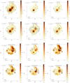 |
Fig. A.1. Upper two rows: flux maps for the [O II] λ3727, [O III] λ5007, Hβ, [N II] λ6584, [S II] λ6718, 6732 gas in the M1931 BCG, lower two rows: equivalent widths in units of [Å] for the same set of emission lines. The white background in all plots correspond to the spaxels with an S/N < 10. The cross shows the location of the AGN. The contours show different levels of flux intensity and EW. |
Appendix B: Emission line velocity maps
Figure B.1 shows the radial velocity and velocity dispersion of the [O II] λ3727, [O III] λ5007, Hβ, [N II] λ6584, [S II] λ6718, 6732 gas in the BCG of the M1931. We observe very similar kinematics for all the strong emission lines in the galaxy spectrum.
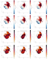 |
Fig. B.1. Kinematics of the warm ionised gas. The panels from the upper two rows display the spatially resolved radial velocity maps for the [O II] λ3727, [O III] λ5007, Hβ, [N II] λ6584, [S II] λ6718, 6732 gas in the BCG of the M1931 galaxy cluster. The colour-bar displays the radial velocity of the gas with respect to the BCG rest frame, measured in [km/s]. The panels from the lower two rows show the spatially resolved velocity dispersion maps for the same emission lines, measured in [km/s]. The white background in all plots correspond to the spaxels with an S/N < 10. The cross shows the location of the AGN. The contours show the Hα flux intensity. |
Appendix C: Physical properties of integrated regions
Figure C.1 shows the white light image of the MUSE sub-cube centred on the BCG of the M1931 galaxy cluster. The contours show the Hα flux intensity. The squares encompass the different CO(1-0) source regions, while the ellipses show the cold dust regions, as defined by Fogarty et al. (2019); see their Figs. 4 and 6. We extracted these eight regions as single integrated spectra and computed the physical properties of the ionised gas, which are listed in Table C.1. The last row of the table contains the physical properties of the ionised gas, as derived from the integrated spectrum of the 90x90 spaxels MUSE sub-cube centred on the BCG. This table lists the flux of the Hα line in units of [10−15 ergs s−1 cm−2], the systemic velocity and velocity dispersion of the Hα gas in [km/s], the electron density ne in [cm−3], the electron temperature Te in [K], the colour excess E(B − V), the ionisation parameter log(U), the SFR in units of [M⊙ yr−1] without correcting for the contribution of LINER-like and AGN emission to the luminosity of the Hα line, as the Davies et al. (2017) decomposition method works only for a spaxel by spaxel analysis and not for integrated regions, and the oxygen abundance 12+log(O/H). The methods and calibrations used to determine the properties of the ionised gas are the same ones used for the spaxel by spaxel analysis. It is worth mentioning that we could not recover the electron density and temperature using the PyNeb tool for regions B, 2, and 3 and for the whole sub-cube, due to the weakness of the temperature-sensitive emission lines and also because in these regions, we are probably observing the luminosity-weighted average of emission lines arising from different volumes with different physical conditions.
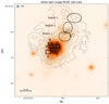 |
Fig. C.1. White light image of the MUSE sub-cube centred on the BCG of the M1931 galaxy cluster. The contours show the Hα flux intensity. The squares encompass the different CO(1-0) source regions, while the ellipses show the cold dust regions, as defined by Fogarty et al. (2019). We have extracted these eight regions as single spectra and computed the most important physical properties of the ionised gas, which are listed in Table C.1. |
Most important physical properties of the ionised gas, as computed for specific regions of the system.
All Tables
Most important physical properties of the ionised gas, as computed for specific regions of the system.
All Figures
|
Fig. 1. HST composite RGB image of the M1931 BCG: the F160W image is shown in red, the F814W in green, and the F390W in blue. The white contours show to the Hα flux intensity, as measured from MUSE. The cross shows the location of the AGN, as identified according to different diagnostic diagrams; see Sect. 5.5. |
| In the text | |
|
Fig. 2. Graphical output of FADO. Upper panel: integrated spectrum of the M1931 BCG orange, as recovered from MUSE. The best-fitting synthetic SED is shown in light-blue, composed of the stellar and nebular continuum emission (dark green and red, respectively). Lower panel: fits to the strongest emission lines, namely, [O II] λ3727, λ3729, Hβ, [O III] λ4959, 5007, Hα, [N II] λ6584, and [S II] λ6718, 6732. |
| In the text | |
|
Fig. 3. Left: spatially resolved Hα emission line map for the BCG of the M1931 galaxy cluster. The colour-bar shows the flux of the Hα line in units of 10−17 ergs s−1 cm−2. Right: Hα equivalent width map measured in Å. The contours correspond to different levels of flux and EW. The white background in both plots corresponds to spaxels with S/NHα < 10. The cross shows the location of the AGN. |
| In the text | |
|
Fig. 4. Comparison between Hα and CO linear normalised flux. Left panel: ratio between Hα and CO(1-0) fluxes. Right panel: ratio between the fluxes of Hα and CO(3-2). The cross shows the location of the AGN. The ellipses in the lower right of both panels depict the beam sizes of the ALMA observations. |
| In the text | |
|
Fig. 5. Left: spatially resolved Hα radial velocity map for the BCG of the M1931 galaxy cluster. The colour-bar displays the radial velocity of the Hα gas with respect to the BCG rest frame, measured in [km/s]. Right: spatially resolved Hα velocity dispersion map measured in [km/s]. The white background in both plots corresponds to spaxels with an S/NHα < 10. The cross shows the location of the AGN. The contours show the Hα flux intensity. |
| In the text | |
|
Fig. 6. Difference between the kinematics of the ionised gas and those of the cold molecular gas. For a better visualisation, we present the zoomed in plots corresponding to a spatial scale of 45 by 45 kpc. Left side: difference between the radial velocity of the Hα gas and the velocity of the CO(1-0) gas (top) and difference between the velocity of the Hα gas and the velocity of the CO(3-2) gas (bottom). Right side: ratio between the Hα velocity dispersion and the CO(1-0) velocity dispersion (top) and ratio between the velocity dispersion of the Hα gas and the velocity dispersion of the CO(3-2) gas (bottom). The cross in all diagrams shows the location of the AGN, as identified according to the different diagnostic diagrams. The ellipses in the lower right of all panels depict the beam sizes of the ALMA observations. |
| In the text | |
|
Fig. 7. Diagnostic diagrams to distinguish the ionisation mechanism of the nebular gas. First row left: BPT diagram (Baldwin et al. 1981) for all spaxels of the MUSE data cube with S/N > 10 in the emission lines used for the diagnostic. First row middle: BPT distribution on the sky showing the spaxels with Seyfert II emission in blue. First row right: BPT distribution on the sky showing the spaxels which fall in the LINER region of the diagnostic diagram in green. Second row left: diagnostic diagram of Veilleux & Osterbrock (1987) using the [O III]/Hβ vs. [S II]/Hα emission line ratios. Second row middle: distribution on the sky showing the Seyfert II emission in blue. Second row right: distribution on the sky showing the LINER emission in green. Third row left: [O III]/Hβ vs [O I]/Hα diagnostic diagram of Veilleux & Osterbrock (1987). Third row middle: distribution on the sky showing the Seyfert II emission in blue. Third row right: distribution on the sky showing the LINER emission in green. In the latter two diagrams, each data point represents a spaxel of the MUSE cube with an S/N > 10 in each emission line used for the diagnostic. The cross from the upper left corner of all three diagnostic diagrams shows the mean error of the flux measurements. The cross in the neighbouring maps show the location of the AGN. |
| In the text | |
|
Fig. 8. Same as Fig. 7, but showing in addition the predictions from the fully radiative shock models of Allen et al. (2008) computed with MAPPINGS V. We consider a pre-shock density of 1 cm−3, shock velocities ranging from 10 to 350 km s−1, and different metallicities. The choice of these shock velocities are motivated by the observed velocity dispersion of the nebular gas. The red lines depict a grid with solar metallicity, the blue ones a grid with twice solar metallicity, the cyan lines one with metallicities from Dopita et al. (2005), the orange ones a grid with Large Magellanic Cloud metallicities, and the purple ones a grid with Small Magellanic Cloud metallicities. The black data-points represent the spaxels of the MUSE cube, with an S/N > 10 in each emission line used for the diagnostic. The grey data-points represent the spaxels of the MUSE cube, from which we have subtracted the contribution from star formation and AGN emission to the total luminosity of each emission line, after applying the decomposition method of Davies et al. (2017). These data-points are representative for pure LINER-like emission. |
| In the text | |
|
Fig. 9. Upper three panels and lower three panels: BPT diagram and the diagnostic diagram of Veilleux & Osterbrock (1987), respectively, with the line ratios extracted from the total emission line fluxes of the individual spaxels. The SF, AGN, and LINER base spectra are depicted as the black square, triangle and circle, respectively. The data points are colour coded according to the fraction of Hα emission attributable to SF (left-hand panels), AGN (middle panels), and ‘LINER’ (right-hand panels), as computed from the spectral decomposition method described in Davies et al. (2017). |
| In the text | |
|
Fig. 10. Maps depicting the fractional contribution of SF (left), AGN (middle), ‘LINER’ (right) to the Hα (first row), [O III] λ5007 (second row), [N II] λ6584 (third row) and [S II] (last row) emission lines, as calculated based on the spectral decomposition method. The colour-bar limit displaying the fractional contribution of each ionising mechanism to the total luminosity of the emission lines was set to 0.8, and not the nominal value of 1, for better visualisation purposes. The cross in all diagrams shows the location of the AGN. |
| In the text | |
|
Fig. 11. Top-left: electron density vs electron temperature diagnostic diagram for the core of the M1931 BCG. For this plot, we use the following diagnostics: [N II] λ 5755/6548, [N II] λ 5755/6584, [S II] λ 6731/6716, [Ar IV] λ 4740/4711, and [O III] λ 4363/5007. The intersection of the curves gives the best fit electron temperature and density. Top-right: same as top-left, but for the Hα tail of the BCG. Bottom-left: spatially resolved electron temperature map for the BCG of the M1931 cluster. The colour bar shows the temperature measured in [K], as computed using the PyNeb tool, from the [N II] λ5755/6584 emission lines. Bottom-right: electron density map as computed using the PyNeb tool, from the [S II] λ6731/6716 doublet. The colour-bar depicts the density in units of cm−3. The contours in both lower panels show the Hα flux intensity, while the cross shows the location of the AGN. |
| In the text | |
|
Fig. 12. Left: colour excess map for the M1931 BCG as computed from the Balmer decrement. Right: ionisation parameter map, as computed from the HII-CH-mistry tool (Pérez-Montero et al. 2014). The cross in all diagrams shows the location of the AGN. The contours show the Hα flux intensity. The white background corresponds to the spaxels with an S/N < 10 in the emission lines of interest. |
| In the text | |
|
Fig. 13. Spatially resolved SFR map calculated from the extinction corrected Hα emission line for each spaxel of the MUSE sub-cube. The colour-bar shows the SFR in units of M⊙ yr−1. The cross shows the location of the AGN, while the contours display the Hα flux intensity. The white background corresponds to the spaxels, which have an S/NHα < 10. |
| In the text | |
|
Fig. 14. Gas phase metallicity (O/H), as computed by the HII-CH-mistry tool. The colour-bar shows the oxygen abundance in units of 12+log(O/H). The cross shows the location of the AGN, while the contours display the Hα flux intensity. The white background corresponds to the spaxels with an S/N < 10 in the emission lines of interest. |
| In the text | |
|
Fig. 15. Star formation history of the M1931 BCG. Upper panel: contribution of the individual SSPs in the best-fitting population vector to the monochromatic luminosity at 6150 Å as a function of age. Lower panel: contribution of the SSPs to the total mass of the system as a function of age. The vertical arrow marks the age when 50% of the present-day stellar mass has been in place. The colour coding in both panels display the metallicities of the SSPs, whose values can be found above the upper plot. The vertical bars represent the 1σ uncertainties. The grey vertical lines connecting the two panels mark the ages of the SSPs. The light-blue shaded area in both panels shows an Akima-smoothed (Akima 1970) version of the SSP contributions. |
| In the text | |
|
Fig. 16. Left: radial velocity of the stars with respect to the systemic velocity of the most central region of the system. Right: velocity dispersion of the stars in the BCG. The colour-bar in both plots depicts the radial velocity and velocity dispersion in units of [km/s]. Due to the low S/N in the stellar continuum, the data needs binning, and we can, therefore, measure the stellar kinematics only in the core of the system. To better visualise the results, we present maps showing just the most central regions of the BCG, corresponding to a spatial scale of 45 × 45 kpc. The white background corresponds to the spaxels, where the S/Nstellar continuum < 10. The cross shows the location of the AGN. |
| In the text | |
|
Fig. 17. Left: difference between the radial velocities of the stars and the Hα gas in the BCG core. Right: ratio between the velocity dispersion of the stars and the Hα gas in the core of the system. To better visualise the results, we present maps showing just the most central regions of the BCG, corresponding to a spatial scale of 45 × 45 kpc. The white background corresponds to the spaxels, where the S/Nstellar continuum < 10. The cross shows the location of the AGN. |
| In the text | |
|
Fig. A.1. Upper two rows: flux maps for the [O II] λ3727, [O III] λ5007, Hβ, [N II] λ6584, [S II] λ6718, 6732 gas in the M1931 BCG, lower two rows: equivalent widths in units of [Å] for the same set of emission lines. The white background in all plots correspond to the spaxels with an S/N < 10. The cross shows the location of the AGN. The contours show different levels of flux intensity and EW. |
| In the text | |
|
Fig. B.1. Kinematics of the warm ionised gas. The panels from the upper two rows display the spatially resolved radial velocity maps for the [O II] λ3727, [O III] λ5007, Hβ, [N II] λ6584, [S II] λ6718, 6732 gas in the BCG of the M1931 galaxy cluster. The colour-bar displays the radial velocity of the gas with respect to the BCG rest frame, measured in [km/s]. The panels from the lower two rows show the spatially resolved velocity dispersion maps for the same emission lines, measured in [km/s]. The white background in all plots correspond to the spaxels with an S/N < 10. The cross shows the location of the AGN. The contours show the Hα flux intensity. |
| In the text | |
|
Fig. C.1. White light image of the MUSE sub-cube centred on the BCG of the M1931 galaxy cluster. The contours show the Hα flux intensity. The squares encompass the different CO(1-0) source regions, while the ellipses show the cold dust regions, as defined by Fogarty et al. (2019). We have extracted these eight regions as single spectra and computed the most important physical properties of the ionised gas, which are listed in Table C.1. |
| In the text | |
Current usage metrics show cumulative count of Article Views (full-text article views including HTML views, PDF and ePub downloads, according to the available data) and Abstracts Views on Vision4Press platform.
Data correspond to usage on the plateform after 2015. The current usage metrics is available 48-96 hours after online publication and is updated daily on week days.
Initial download of the metrics may take a while.