| Issue |
A&A
Volume 689, September 2024
|
|
|---|---|---|
| Article Number | A315 | |
| Number of page(s) | 15 | |
| Section | Extragalactic astronomy | |
| DOI | https://doi.org/10.1051/0004-6361/202450715 | |
| Published online | 20 September 2024 | |
The MAGPI survey: The interdependence of the mass, star formation rate, and metallicity in galaxies at z ∼ 0.3
1
University of Vienna, Department of Astrophysics, Türkenschanzstrasse 17, 1180 Vienna, Austria
2
Univ Lyon1, CNRS, Centre de Recherche Astrophysique de Lyon, 69230 Saint-Genis-Laval, France
3
Research School of Astronomy and Astrophysics, Australian National University, Cotter Road, Weston Creek, ACT 2611, Australia
4
ARC Centre of Excellence for All Sky Astrophysics in 3 Dimensions (ASTRO 3D), Canberra, ACT 2611, Australia
5
International Centre for Radio Astronomy (ICRAR), M468, The University of Western Australia, 35 Stirling Highway, Crawley, WA 6009, Australia
6
Sydney Institute for Astronomy, School of Physics, University of Sydney, Sydney, NSW 2006, Australia
7
School of Physics, University of New South Wales, Sydney, NSW 2052, Australia
8
School of Mathematical and Physical Sciences, Macquarie University, Sydney, NSW 2109, Australia
9
School of Mathematics and Physics, University of Queensland, Brisbane, QLD 4072, Australia
10
University of Strasbourg, CNRS UMR 7550, Observatoire astronomique de Strasbourg, 67000 Strasbourg, France
11
University of Strasbourg Institute for Advanced Study, 5 allée du Général Rouvillois, 67083 Strasbourg, France
12
SISSA International School for Advanced Studies, Via Bonomea 265, 34136 Trieste, Italy
13
Department of Physics and Astronomy, University of the Western Cape, Cape Town 7535, South Africa
14
Universitäts-Sternwarte, Fakultät für Physik, Ludwig-Maximilians-Universität München, Scheinerstr. 1, 81679 München, Germany
15
Instituto de Astrofísica e Ciências do Espaço – Centro de Astrofísica da Universidade do Porto, Rua das Estrelas, 4150-762 Porto, Portugal
Received:
14
May
2024
Accepted:
3
July
2024
Abstract
Aims. Star formation rates (SFRs), gas-phase metallicities, and stellar masses are crucial for studying galaxy evolution. The different relations resulting from these properties give insights into the complex interplay of gas inside galaxies and their evolutionary trajectory and current characteristics. We aim to characterize these relations at z ∼ 0.3, corresponding to a 3–4 Gyr lookback time, to gather insight into the galaxies’ redshift evolution.
Methods. We utilized optical integral field spectroscopy data from 65 emission-line galaxies from the MUSE large program MAGPI at a redshift of 0.28 < z < 0.35 (average redshift of z ∼ 0.3) and spanning a total stellar mass range of 8.2 < log(M*/M⊙) < 11.4. We measured emission line fluxes and stellar masses, allowing us to determine spatially resolved SFRs, gas-phase metallicities, and stellar mass surface densities. We derived the resolved star formation main sequence (rSFMS), resolved mass metallicity relation (rMZR), and resolved fundamental metallicity relation (rFMR) at z ∼ 0.3, and compared them to results for the local Universe.
Results. We find a relatively shallow rSFMS slope of ∼0.425 ± 0.014 compared to the expected slope at this redshift for an ordinary least square (OLS) fitting routine. For an orthogonal distance regression (ODR) routine, a much steeper slope of ∼1.162 ± 0.022 is measured. We confirm the existence of an rMZR at z ∼ 0.3 with an average metallicity located ∼0.03 dex above the local Universe’s metallicity. Via partial correlation coefficients, evidence is found that the local metallicity is predominantly determined by the stellar mass surface density and has a weak secondary (inverse) dependence on the SFR surface density ΣSFR. Additionally, a significant dependence of the local metallicity on the total stellar mass M* is found. Furthermore, we find that the stellar mass surface density Σ* and M* have a significant influence in determining the strength with which ΣSFR correlates with the local metallicity. We observe that at lower stellar masses, there is a tighter correlation between ΣSFR and the gas-phase metallicity, resulting in a more pronounced rFMR.
Key words: galaxies: abundances / galaxies: evolution / galaxies: ISM / galaxies: star formation
Corresponding author; This email address is being protected from spambots. You need JavaScript enabled to view it. .
© The Authors 2024
 Open Access article, published by EDP Sciences, under the terms of the Creative Commons Attribution License (https://creativecommons.org/licenses/by/4.0), which permits unrestricted use, distribution, and reproduction in any medium, provided the original work is properly cited.
This article is published in open access under the Subscribe to Open model. This email address is being protected from spambots. You need JavaScript enabled to view it. to support open access publication.
1. Introduction
The processes governing galaxy evolution set the local and global gas-phase chemical abundances and stellar masses of galaxies (Madau & Dickinson 2014; Lilly et al. 2013). The rate of inflowing and outflowing gas, feedback processes such as stellar winds and supernovae (SNe), and the rate at which gas is recycled within galaxies determine the abundance of metals, measured as the gas-phase metallicity, and star formation activity (Péroux & Howk 2020). Gas-phase metallicity is traced via strong ionized gas emission lines (Kewley et al. 2019), which are correlated with the amount of metals produced in past stellar generations (Maiolino & Mannucci 2019). Inflowing pristine (metal-poor) gas from the intergalactic medium (IGM) both dilutes the overall gas content and increases the star formation rate (SFR) (Tumlinson et al. 2017). Stellar evolution plays a role in this gas cycle by providing chemically enriched gas to the interstellar medium (ISM) through SN explosions and stellar winds. High metallicity gas can leave the galaxy through galactic winds to enrich the circumgalactic medium (CGM). The gas inside galaxies is recycled multiple times and undergoes numerous stellar generations. Dust is created and destroyed, which captures and releases metals. The presence of a central active galactic nucleus (AGN) impacts the properties of the ISM and the CGM, either by heating the gas or by removing it through AGN-driven winds, and both of these effects can impede star formation (Lilly et al. 2013; Peng & Maiolino 2014).
This interdependence between ionized gas properties has been studied for decades. It is essential to investigate to better understand the cosmic baryon cycle, which defines the star formation activity and metal content present in the gas of galaxies (Péroux & Howk 2020). One of these relations is the correlation between gas-phase metallicity and stellar mass, the so-called mass-metallicity relation (MZR, see e.g., Tremonti et al. 2004; Kewley & Ellison 2008; for a review Maiolino & Mannucci 2019). This correlation was first defined as a metallicity versus luminosity relation by Lequeux et al. (1979). An increase in stellar mass correlates with an increase in metallicity until the relation flattens out at high stellar masses. Tremonti et al. (2004) studied this relation using 53 000 star-forming galaxies at z = 0.1 from the Sloan Digital Sky Survey (SDSS; Kollmeier et al. 2019) and found that the MZR has a ∼0.1 dex scatter spanning three orders of magnitude in stellar mass and a factor of ten in metallicity. This relation has been studied for the local Universe and redshifts up to z ∼ 10 (Maiolino et al. 2008; Lamareille et al. 2009; Mannucci et al. 2010; Maier et al. 2014; Cresci et al. 2019; Curti et al. 2019, 2022; Nakajima et al. 2023). An evolution with redshift has been observed: high redshift galaxies are more metal-poor than local galaxies (Tremonti et al. 2004; Savaglio et al. 2005; Maiolino et al. 2008; Gao et al. 2018; Sanders et al. 2021). The MZR’s redshift evolution is commonly attributed to galaxies in the local Universe having had a longer time to produce and assemble metals than galaxies at high redshifts.
Another correlation is established between the SFR and the stellar mass of a galaxy: the star formation main sequence (SFMS, see e.g., Brinchmann et al. 2004; Noeske et al. 2007; Whitaker et al. 2012; Speagle et al. 2014; Renzini & Peng 2015). Star-forming galaxies inhabit a near-linear relation in the SFR versus stellar mass space. Galaxies that experience star formation enhancements or suppression are situated above or below this line, respectively (Noeske et al. 2007). The SFMS is also observed to evolve with redshift: galaxies at a given M* have higher SFRs at higher redshifts (Speagle et al. 2014; Pearson et al. 2018; Leslie et al. 2020).
Connecting all three properties (stellar mass, SFR, and gas-phase metallicity) establishes a three-dimensional relation: the fundamental metallicity relation (FMR, see e.g., Mannucci et al. 2010; Lara-López et al. 2010; Cresci et al. 2019; Curti et al. 2019, 2024; Pistis et al. 2024; Li et al. 2024), which is typically not observed to evolve with redshift. For a given stellar mass, galaxies with higher SFRs exhibit a lower metallicity. Ellison et al. (2008), who first discovered this anti-correlation, used over 40 000 galaxies from the SDSS survey to investigate the correlation between the specific star formation rate (sSFR), which is defined as sSFR = SFR/M*, and the gas-phase metallicity. They concluded that galaxies with a higher sSFR have systematically lower metallicities of up to 0.2 dex at a fixed stellar mass. Their study also discussed some possible origins for this relationship between the SFR and metallicity, including environmental effects, star formation efficiencies, infall of metal-poor gas, and galactic winds. This anticorrelation was later confirmed by Mannucci et al. (2010), who investigated the relationship between the SFR, gas-phase metallicities, and stellar masses of a large sample of galaxies ranging over redshifts of z = 0 − 2.5, and Lara-López et al. (2010), who also conducted a study of these three properties for star-forming galaxies of the SDSS survey over a redshift range of 0.04 < z < 0.1. Both studies concluded that the galaxies populate a three-dimensional plane, the FMR. Mannucci et al. (2010) observations also show that the relation is more robust for low-mass galaxies and that the metallicity ceases to depend on the SFR at high stellar masses.
In recent years, the FMR has been a great topic of discussion. Publications such as Sánchez et al. (2013) and Barrera-Ballesteros et al. (2016) have questioned the relation’s existence. Support has been found in the works of Lara-López et al. (2010), Mannucci et al. (2010), Salim et al. (2014). Currently, the largest studies of the FMR have been done using local galaxies, but investigations at higher redshifts have been made (Cresci et al. 2012, 2019; Curti et al. 2022, 2024; Nakajima et al. 2023). Studies toward higher redshifts where the S/N and overall spatial resolution are much lower than for local galaxies are still scarce. With the advent of the most recent generation of NIR IFU spectrographs, such as VLT/ERIS and JWST/NIRSpec, and more extensive surveys conducted via optical IFU spectrographs, such as VLT/MUSE, this gap may now be addressed. Some studies in the IR using early-release JWST/NIRSpec data have already been performed. For example, Nakajima et al. (2023) investigated the FMR and redshift evolution of the MZR at z = 4 − 10 from 135 galaxies using JWST/NIRSpec data. They find that only a small MZR evolution is observed from z = 2 − 3 to z = 4 − 10 while the FMR shows no significant evolution up to z ∼ 8.
Cresci et al. (2012, 2019) also studied the redshift evolution of the FMR and find an absence of changes over cosmic time. On the contrary, Garcia et al. (2024) studied the FMR via Illustris (Vogelsberger et al. 2014), Illustris The Next Generation (IllustrisTNG; Pillepich et al. 2018), and Evolution and Assembly of GaLaxies and their Environment (EAGLE; Schaye et al. 2015) simulations. Their results are consistent with a “weak” FMR with a non-negligible redshift evolution.
In recent years, spatially resolved spectroscopy of galaxies from surveys of the local Universe (for a review see Sánchez 2020) such as the Calar Alto Legacy Integral Field Area (CALIFA; Sánchez et al. 2012) survey, Mapping Nearby Galaxies at APO (MaNGA; Bundy et al. 2015) survey, and Sydney-AAO Multiobject Integral-field spectrograph (SAMI; Croom et al. 2021) survey have become more accessible for larger samples, making it possible to study these relations on kpc-scales. Resolved relations can be established by substituting the measured parameters for surface densities. The resolved star formation main sequence (rSFMS, see e.g., Cano-Díaz et al. 2016; Ellison et al. 2018; Medling et al. 2018; Jafariyazani et al. 2019; Yao et al. 2022; Baker et al. 2021) describes the relation between stellar mass surface density, Σ*, and SFR surface density, ΣSFR. Similarly, a resolved mass metallicity relation (rMZR) has been observed as well by relating Σ* and the local metallicity (Rosales-Ortega et al. 2012; Sánchez et al. 2013; Barrera-Ballesteros et al. 2016; Yao et al. 2022). Studies by Sánchez-Menguiano et al. (2019), Baker et al. (2022), and Li et al. (2024) have found evidence for a resolved FMR. Nonetheless, clear evidence for the existence of an rFMR even at z ∼ 0, where the most extensive IFU studies have been conducted so far, has yet to be found (e.g., Barrera-Ballesteros et al. 2016).
Spatially resolved investigations at intermediate redshifts have been conducted (Jafariyazani et al. 2019; Yao et al. 2022). For instance, Yao et al. (2022) analyzed the spatially resolved MUSE data of ten star-forming galaxies at z ∼ 0.26. They find consistent results for an rMZR and rSFMS, but no clear evidence for an rFMR.
More extensive spatially resolved studies toward higher redshifts are needed to get a clear picture of the rMZR’s redshift evolution and to find evidence of whether or not an rFMR exists at intermediate redshifts around z ∼ 0.3 (3–4 Gyr lookback time). In this context, we aim to bridge this gap between the local Universe and higher redshifts by investigating galaxies spatially resolved ionized gas relations via the Middle Ages Galaxy Properties with Integral field spectroscopy (MAGPI; Foster et al. 2021) survey1 at a 3–4 Gyr lookback time between cosmic noon and the local Universe.
This paper is structured as follows. In Sect. 2, we discuss the survey and data products used in this work and describe our sample selection criteria. In Sect. 3, we discuss how we measure our physical quantities. Our results are presented in Sect. 4 and discussed in Sect. 5. Finally, we summarize and conclude our results in Sect. 6. Throughout this paper, we assume a Chabrier (2003) initial mass function (IMF) and adopt a flat ΛCDM cosmology with H0 = 70.0 km s−1 Mpc−1, Ωm = 0.3, and Ωλ = 0.7.
2. Data
2.1. The MAGPI survey
The MAGPI survey (Foster et al. 2021) is a VLT/MUSE large program (Program ID: 1104.B-0536) targeting galaxy environments at redshifts 0.28 < z < 0.35, corresponding to 3–4 Gyr lookback times. MAGPI’s primary goal is to obtain spatially resolved spectroscopic properties of the galaxies’ stars and ionized gas to explore the different mechanisms shaping the morpho-kinematics of today’s massive galaxies at a crucial time in their evolution. Representing an extension to already existing low-redshift IFU surveys like SAMI and MANGA, MAGPI provides comparable spatial resolutions but at nearly twice the lookback time, thus filling a gap at this intermediate redshift range.
The survey targets 60 primary galaxies, which were selected based on a stellar mass of M* > 7 × 10¹⁰ M⊙, and ∼100 satellites in a wide range of environments. In total, 56 out of the 60 primary targets were selected from the fields G12, G15, and G23 stemming from the Galaxy and Mass Assembly (GAMA, Driver et al. 2011) survey. The other four outstanding primary targets were taken from archival MUSE observations of Abell 370 and Abell 2744 fields.
The observations are conducted with the MUSE Wide Field Mode within a wavelength range of 4650 Å − 9300 Å and a spectral sampling of 1.25 Å. Each MAGPI field covers a field-of-view of roughly 1′×1′ and is centered on a primary target. A spatial sampling of 0.2″ per pixel and an average image quality of 0.65″ FWHM in the V-band is achieved (Foster et al. 2021). Each field is observed over six observing blocks with an exposure time of 2 × 1320 s each, resulting in an integrated time of 4.4 h per field. Ground-layer adaptive optics (GLAO) alleviates atmospheric seeing, resulting in a 270 Å wide gap within the galaxies observed spectra at 5780 − 6050 Å caused by the GALACSI sodium laser notch filter. A detailed explanation of the data reduction and various spatially resolved map creations are discussed in Mendel et al. (in prep.). Currently, observations for MAGPI are ongoing, with 42 out of 60 fields (∼70% completion rate) having been observed and fully reduced.
For our galaxy selection, we utilized an emission line catalog of the integrated galaxy spectra of all observed targets. This emission line product is fully described in Battisti et al. (in prep.). Emission lines are measured via GIST (Bittner et al. 2019), which is a Python wrapper for pPXF (Cappellari & Emsellem 2004; Cappellari 2017) and GANDALF (Sarzi et al. 2017). For more details on the MAGPI-derived emission line fluxes, see also Mun et al. (2024). Morphological parameters are derived from pseudo-i-band images produced from the MUSE data. Half light radii Re and semi-major axis containing 90% of the flux R90 are measured using the Profound R Package (Robotham et al. 2018). The total stellar masses M* used to introduce our sample in Fig. 1 were computed via ProSpect (Robotham et al. 2020). We also use MAGPI’s spectroscopic redshifts derived via MARZ (Hinton et al. 2016).
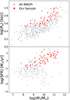 |
Fig. 1. Distribution of our selected sample. Top: Mass-size diagram for our selected galaxies (red) vs. the entire MAGPI catalog within the same redshift range of 0.28 < z < 0.35 as us (gray). Stellar masses were taken from MAGPI’s ProSpect catalog and effective radii from MAGPI’s Profound catalog. Bottom: Mass-SFR diagram via SFRs derived from integrated Hα fluxes taken from MAGPI’s GIST measurements. |
2.2. Selection of galaxies and spaxels
This work focuses on a sample of galaxies selected based on several criteria. First, galaxies must lie within MAGPI’s primary redshift range (0.28 < z < 0.35), which results in 393 available galaxies. Secondly, we select galaxies based on the S/N of their integrated spectrum of the following emission lines: Hβ, [OIII]λ 5007, [NII]λ6583, and Hα. Galaxies must have a S/N > 5 in all four emission lines. Thirdly, galaxies must have an effective radius Re in i-band of Re > 0.7″, making it 0.05″ larger than the spatial resolution of the MUSE observations. Fourthly, the galaxy should not be at the edge of the MUSE field or be cut off. Lastly, we remove highly inclined galaxies with a minor (b′) to major (a′) axis ratio of b′/a′< 0.35 to avoid strong inclination and extreme extinction corrections. Following all the selection criteria, we are left with 65 galaxies.
In Fig. 1, we show the distribution of our selected sample as mass-size and mass-SFR diagrams and compare them to the entire MAGPI sample within the same redshift range. The star formation rates shown here were computed only for galaxies with Hα measurements (z < 0.42 for the MUSE spectral window) following the equations described in Sect. 3.2 and corrected for intrinsic extinction as described in Sect. 3.1. The Hα flux measurements were taken from MAGPI’s integrated emission line catalog using GIST (Battisti et al., in prep.).
We extracted spaxels from the MAGPI cubes via the MUSE Python Data Analysis Framework (MPDAF; Bacon et al. 2016) and corrected for Galactic foreground extinction using the noao onedspec deredden routine from the Image Reduction and Analysis Facility (IRAF; Tody 1986), which is based on the empirical selective extinction function of Cardelli et al. (1989). We adopted a fixed ratio of extinction in V-band (= 5550 Å), AV, to color excess E(B − V) of RV = 3.1, and adopted the galaxies’ corresponding total extinction values AV from Schlafly & Finkbeiner (2011). We selected spaxels based on an S/N > 3 criterion for the Hβ, [OIII]λ5007, [NII]λ6583, and Hα emission lines to ensure an accurate line detection. We chose this criterion as it corresponds to a certain flux limit that allows us to get accurate measurements.
Only spaxels falling within the star-forming region of the [NII]/Hα versus [OIII]/Hβ Baldwin–Philips–Terlevich (BPT, Baldwin et al. 1981) diagnostic diagram employing the empirical line calibration by Kauffmann et al. (2003) (see Fig. 2) were taken into account. We did not correct the empirical and theoretical line calibrations for redshift due to the only faint effect present at our target redshift of z ∼ 0.3 or corrected for underlying stellar absorption, which could result in a slight overestimation of the [OIII]/Hβ ratio. In total, 9825 spaxel fulfilled our S/N criterion, while 6299 were classified as SF-spaxel and utilized for the following spatially resolved analysis.
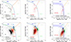 |
Fig. 2. Global and spatially resolved diagnostic diagrams. Top: Diagnostic diagrams by Baldwin et al. (1981) (left), Veilleux & Osterbrock (1987) (middle), and Lamareille (2010) (right) for the galaxies’ integrated flux measurements. The gray error bars in the top right indicate all diagrams’ mean flux ratio errors along the x- and y-axis. In the case of the Lamareille (2010) diagram, only galaxies with [OII]λ3727 measurements via FADO were included. Bottom: The same diagnostic diagram of all spaxels satisfying the S/N > 3 criteria in all four emission lines – [OIII]5006 Å, Hβ, Hα, and [NII]6585 Å. The diagnostic diagram by Baldwin et al. (1981) distinguishes between star-forming (black), composite (red), AGN (blue), and LINER (green) emission while the diagrams by Lamareille (2010) and Veilleux & Osterbrock (1987) both only differentiate between star-forming and possibly composite (red), AGN (blue), and LINER (green). |
3. Methods
3.1. Emission line fits and stellar masses
We determined emission line fluxes and stellar masses via the population spectral synthesis code Fitting Analysis using Differential evolution Optimization (FADO; Gomes & Papaderos 2017) using the library of simple stellar population (SSP) spectra from Bruzual & Charlot (2003). FADO already corrects fluxes for underlying stellar absorption. FADO only provides formal errors in all quantities, meaning that the errors are based on the goodness of the fits and the convergence of the different evolutionary threads, resulting in the best-fitting solution obtained via differential genetic optimization. These errors should be seen as low limits to the quantities’ true limits, most specifically, for the stellar masses. As a consistency check, we also computed emission line fluxes via MPDAF (Bacon et al. 2016) and obtained measurements done via GIST (Bittner et al. 2019), and found good agreement between the measurements yielded by the three different tools.
We corrected all emission lines for dust extinction via the Hα/Hβ Balmer decrement following the equations introduced by Calzetti (2001), which assume a Cardelli et al. (1989) extinction curve, assuming an intrinsic flux ratio of Hα/Hβ = 2.86 and RV = 3.1. Lastly, we corrected surface densities for inclination by assuming an infinitely thin disk and a simplified inclination angle of cos(Θ) = b′/a′:
 (1)
(1)
We note that a′ and b′ refer to the major and minor axes.
3.2. Star formation rate surface densities
The star formation rates were calculated via the extinction-corrected Hα luminosity using the SFR calibration from Kennicutt (1998) assuming a Salpeter IMF:
 (2)
(2)
We converted SFRs from a Salpeter IMF to Chabrier IMF via the conversion factor from Driver et al. (2013): MChabrier = MSalpeter/1.53. We converted spatially resolved star formation rates into surface densities by dividing each spaxel’s SFR by its area: ΣSFR = SFR/A(M⊙ yr−1 kpc−2). We record an average error of 0.04 dex for log(ΣSFR).
3.3. Gas-phase metallicities
We utilized an optical strong-line calibration to measure gas-phase metallicities. We used the O3N2 index, which is defined as
![Mathematical equation: $$ \begin{aligned} \mathrm{O3N2} = \log {\left( \frac{[\mathrm{OIII}]\lambda 5007/\mathrm{H}\beta }{[\mathrm{NII}]\lambda 6583/\mathrm{H}\alpha } \right)} \end{aligned} $$](/articles/aa/full_html/2024/09/aa50715-24/aa50715-24-eq3.gif) (3)
(3)
and the calibration by Marino et al. (2013) with O3N2 ranging from –1.1 to 1.7, corresponding to a range in metallicity of 8.17 ≲ 12 + log(O/H)≲8.77:
 (4)
(4)
The average error for the metallicity calibration derived via oxygen with this O3N2 diagnostic is ∼0.08 dex. For our sample, 39 spaxels fall outside of the metallicity range defined by Marino et al. (2013), and we henceforth excluded them from our analysis.
4. Results
In the following sections, we present several results to explore the SFMS, MZR, and FMR in the MAGPI sample. We compare these results to previous works. Differences in IMFs between our work and others have been adjusted. All emission lines used in this analysis are corrected for intrinsic extinction based on the Balmer decrement as described in Sect. 3.1, and we selected only spaxels classified as star-forming in the BPT diagram by Baldwin et al. (1981) using the Kauffmann et al. (2003) empirical separation line.
4.1. Ionization sources
4.1.1. Diagnostic diagrams
The different ionization sources present in our sample of galaxies were investigated via three diagnostic diagrams, which use a set of four strong emission lines. By applying these diagnostics to our spatially resolved emission line flux measurements, we can reliably distinguish between star-forming (SF), Seyfert (AGN), low ionization nuclear emission-line regions (LINER), and composite galaxies or spaxels. Composite galaxies or spaxels are regions where photoionization is powered by star formation, an AGN, and possibly other mechanisms responsible for LINER emissions, such as shocks or cosmic rays. We utilized the classical BPT diagram by Baldwin et al. (1981) which makes use of the [OIII]/Hβ and [NII]/Hα emission line ratios, the [OIII]/Hβ versus [SII]/Hα diagnostic diagram of Veilleux & Osterbrock (1987), as well as the [OIII]/Hβ versus [OII]/Hβ diagram of Lamareille (2010).
Figure 2 shows the results for the classical BPT diagram on the left-hand side: the results on the top are for integrated galaxy values, while the results shown at the bottom are for a spaxel-by-spaxel analysis. The differently colored lines within the diagram act as a separation between the different ionizing mechanisms. The solid blue curve of Kewley et al. (2001) depicts the theoretical line that separates SF and composite galaxies or spaxels from AGN and LINER galaxies or spaxels. In contrast, the dashed green line of Kauffmann et al. (2003) is an empirical calibration that further distinguishes between SF and composite galaxies or spaxels. Additionally, the solid orange curve of Schawinski et al. (2007) represents the separation line between AGN and LINER galaxies or spaxels. Our results show a sample dominated by star-forming (64%) and composite (27%) spaxels, and the remaining 9% spaxels are classified as AGN or LINER.
The middle panel of Fig. 2 depicts the [OIII]/Hβ versus [SII]/Hα diagnostic diagram of Veilleux & Osterbrock (1987). Here, the solid blue curve represents the theoretical separation curve of Kewley et al. (2001), which separates SF galaxies or spaxels from AGNs and LINERS. In contrast, the solid orange curve represents the separation line of Schawinski et al. (2007), which helps distinguish between AGN and LINER galaxies or spaxels. Again, our sample is shown to be dominated by spaxels ionized by star formation, with roughly 82% classified as such. Compared to the 3% of LINER emission classified by the BPT diagram, 12% of all spaxels amount to LINER emission in the Veilleux & Osterbrock (1987) diagram.
Lastly, the right panel of Fig. 2 depicts the Lamareille (2010) diagnostic diagram, which is specifically designed to use emission lines from the bluer side of galaxies spectra to avoid them being redshifted out of the wavelength range of optical spectrographs. It can, therefore, distinguish between star-forming and AGN galaxies or spaxels at intermediate redshifts (z > 0.3) where the danger of the [NII], [SII], and Hα emission lines not being observable is present. The solid blue line separates AGN from star-forming galaxies or spaxels. Its 0.1 dex uncertainty regions are also shown as dashed blue lines. Furthermore, an empirical line to distinguish between LINER and AGN galaxies or spaxels is also introduced. Both of these lines were taken from Lamareille (2010). Again, our sample is observed to be dominated by SF spaxels.
Within the global BPT diagram shown in the top left of Fig. 2, 70% of galaxies are classified as SF. This percentage increases to 80% for both the Veilleux & Osterbrock (1987) diagram (top middle) and Lamareille (2010) diagram (top right). To conclude, in both the spaxel-by-spaxel and global analyses via integrated galaxy fluxes, we confirm that SF and composite galaxies dominate our sample.
4.1.2. Spectral decomposition method
We also applied the spectral decomposition method from Davies et al. (2016, 2017) to gain deeper insights into the ionizing sources dominating our sample. This method lets us dissect and filter out the contributions from star formation, AGN activity, and LINER emission to the luminosity of selected emission lines of individual spaxels. The method is based on the diagnostic diagram by Baldwin et al. (1981). Here, we first have to choose three basis spectra, each representing one of the three ionization sources: star formation, AGN emission, and LINER emission. In our case, we opted not to select specific spaxels as base spectra, as we analyzed our entire sample simultaneously and did not want the fluxes from one specific galaxy to have such a significant impact on the outcome. Instead, we elected to compute the median fluxes of the four emission lines [OIII], Hβ, [NII], and Hα in each BPT region representing the three ionizing mechanisms. For instance, we can compute a star formation base spectrum via the line ratios computed from the median fluxes taken over all spaxels in the star-forming region of the BPT diagram. To check whether our chosen median base spectra accurately represent each ionization mechanism, we also computed and plotted them within the diagnostic diagram from Veilleux & Osterbrock (1987) and found good agreement with their respective location within the diagram’s different sections and their location within the BPT diagram. Furthermore, the second step in this decomposition method is to apply the following linear superposition equation defined by Davies et al. (2017):
 (5)
(5)
where Li(j) refers to the luminosity of any emission line i of any spaxel j. Li(HII), Li(AGN), and Li(LINER) are the luminosities for any emission line i of the star-forming, AGN, and LINER base spectra. m is the superposition coefficient for star formation, n for AGN emission, and k for LINER emission. These three coefficients vary between spectra but are the same for all emission lines within a spectrum. In summary, this equation represents the linear superposition of the line luminosities of the different ionizing mechanisms that make up every emission line of every spaxel. We computed the superposition coefficients by imposing a least-square minimization on Eq. (5) via the Levenberg-Marquardt nonlinear fitting routine from lmfit (Newville et al. 2016). The luminosities in Eq. (5) represent the extinction-corrected luminosities of the following four emission lines: [OIII]λ5007, Hα, [NII]λ6584, and [SII]λ6718,6731. Afterward, we utilized the superposition coefficients to calculate the luminosities of the emission lines of interest associated with star formation, AGN activity, and LINER emission by simply multiplying each superposition coefficient with its respective basis spectrum and the Hα luminosity. We multiply with LHα as in an earlier step, we normalize both the luminosities Li(j) on the left-hand side of Eq. (5) and the luminosities of the basis spectra to an Hα luminosity of 1.
We note that the resulting luminosities can be used for computing SFRs, which is discussed in Sect. 4.3. However, since all spaxels are scaled versions of the star-forming regions basis spectrum, it is not possible to compute flux ratios, ergo gas-phase metallicities, as all spaxels would have very similar or the same value. Additionally, potential limitations of the spectral decomposition method stem from the dependence of emission line luminosities on various factors, including the mix of ionization mechanisms and the metallicity and ionization parameter of the gas (Davies et al. 2017). On the contrary, this method is advantageous as it enables the inclusion of more spaxels than the conventional method of only SF spaxels. Our analysis encompassed 9475 spaxels, a substantial increase over the 6299 spaxels included via the traditional method.
Examining the effectiveness of the spectral decomposition approach from Davies et al. (2017) involves assessing the consistency in emission fractions attributed to individual ionization mechanisms across line ratios. This consistency should ideally peak at the line ratios corresponding to the relevant basis spectrum and gradually decline as the line ratios approach those of another basis spectrum. In this sense, we should be able to observe that the different empirical and theoretical lines used to distinguish between the ionization mechanisms match with a decrease in the fractional contributions. Results are shown in Fig. 3 where the upper three panels present the BPT diagram by Baldwin et al. (1981) and the lower three panels show the diagnostic diagram by Veilleux & Osterbrock (1987). The data points are color-coded according to their fractional contribution of SF (left), AGN (middle), and LINER (right) to the Hα emission line.
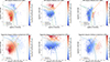 |
Fig. 3. Diagnostic diagrams by Baldwin et al. (1981) (top row) and Veilleux & Osterbrock (1987) (bottom row) with emission line flux ratios extracted from the total emission line fluxes of the individual spaxels. The lime green icons indicate the base spectra for star formation (square), AGN emission (circle), and LINER emission (triangle). Our data points shown here are color-coded using the fraction of Hα emission that is ascribable to SF (left), AGN emission (middle), and LINER emission (right). The data points are smoothed over via LOESS (Cappellari et al. 2013). |
The line calibration by Kauffmann et al. (2003) aligns quite well with the fractional contribution of SF to Hα. Most notably, the contribution of AGN is strong throughout the entire AGN region of both diagnostic diagrams and extends deep into the LINER region. Lastly, similar to the SF region, the spaxels with high contribution from LINER emission are also well contained via the Kewley et al. (2001) and Schawinski et al. (2007) lines.
It is worth mentioning that in the case of the contributions from AGN and LINER, we had to omit a significant amount, approximately a third of all spaxels, from Fig. 3 for which this method could not produce meaningful values as the resulting fractional contributions were too close to zero. These spaxels lie within the parts of the diagrams that are furthest away from the respective emission. For example, in the top right panel showing the fractional contribution from LINER emission to the Hα emission line, some spaxels of the AGN and SF regions were omitted.
We conclude from the spectral decomposition method that our sample is predominately dominated by SF with additional contributions from LINER and AGN. The average fractional contribution of star formation to the Hα emission line accounts for ∼50 − 60% of the ionized gas emission, whereas both AGN and LINER emission account for roughly ∼20% each.
4.2. Global relations
This section briefly summarizes the resulting global versions of the SFMS and MZR relations. We implemented two approaches to obtain global values for the stellar mass M* and SFR. First, we used the integrated spectrum of each galaxy and processed it through FADO as described in Sect. 3.1, which gives us a total stellar mass estimate as well as a global Hα flux measurement, which is then used to compute a global SFR for each galaxy as described in Sect. 3.2. Secondly, we computed the sum of all resolved spaxel values that fulfill our S/N criteria within each galaxy to obtain measurements for global properties.
Generally, SFRs obtained by totaling the resolved values are expected to be smaller than integrated SFRs. As with the former method, some spaxels are excluded from the calculations, resulting in a weaker overall flux, ultimately underestimating the global SFR. Indeed, we observe an average difference of 2.5 M⊙ yr−1 between integrated and total resolved global SFRs. Additionally, integrated and total resolved stellar masses obtained via FADO were compared to those obtained via ProSpect by MAGPI team members. We find that ProSpect masses are, on average, 0.04 dex higher than the integrated FADO masses and 0.14 dex higher than the total resolved FADO masses. In the following sections concerning the spatially resolved results, we applied global integrated measurements whenever global parameters were used for the stellar mass M* and SFR.
4.2.1. Star formation main sequence
The top panel of Fig. 4 depicts the global SFMS for both the integrated values (green circles) and total resolved values (blue triangles). Furthermore, we also utilized two different fits for comparisons: the function by Renzini & Peng (2015), which evaluated the SFMS based on SDSS data, and by Boogaard et al. (2018), which utilized SFRs derived from Hα and Hβ (only for galaxies with z > 0.42) and is defined for a redshift range of 0.1 < z < 0.5. Both calibrations were derived via integrated measurements and also best align with our integrated values. Additionally, a subgroup of galaxies exhibits relatively low SFRs according to their total resolved values, especially when compared to their integrated measurements. A possible explanation could be that many of their spaxels did not pass our S/N criteria within these galaxies, resulting in their being omitted when computing global parameters.
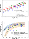 |
Fig. 4. Global relations for our sample. Top: Global SFMS. The green circles depict the integrated measurements for SFR and M*, while the blue triangles represent the sum of all the resolved spaxel values within each galaxy. The dashed black line represents the fit from Renzini & Peng (2015). The dash-dotted black line shows the fit from Boogaard et al. (2018). Our own linear fit results are shown in red with its ∼0.4 dex scatter as a dotted red line. Bottom: Global MZR. The integrated 12 + log(O/H) as green circles are calculated using the integrated flux measurements, while the blue triangles represent the median resolved gas-phase metallicity of each galaxy. The dashed black line and 0.102 dex scatter in orange represents the MZR fit from Sánchez et al. (2019) while the dotted black line and 0.06 dex scatter in blue stems from Sánchez et al. (2017). |
We applied an ordinary linear least-square fitting and utilized the following function in log-log space considering individual errors:
 (6)
(6)
This results in the following fit: b = 0.481 ± 0.242 and a = −4.749 ± 2.412. We measure a 1σ scatter, derived by calculating the standard deviation of the residual between the observed and fitted log(SFR), of ∼0.4 dex.
4.2.2. Mass metallicity relation
The bottom panel of Fig. 4 shows the global gas MZR. Corresponding to the resolved stellar mass measurements, gas-phase metallicities of each galaxy are their median metallicity over all spaxel values. Integrated gas-phase metallicities were computed by taking the integrated flux measurements. In this case, no overall significant difference in the distribution of the data points between median and integrated values is apparent, most likely due to shallow metallicity gradients within this sample where removing low S/N spaxels does not alter the overall line ratios. We compare our results to those found by Sánchez et al. (2017), who investigated the MZR via CALIFA data at z ∼ 0, and by Sánchez et al. (2019), who investigated the MZR via SAMI data at 0.005 < z < 0.1. Both utilized the same 12 + log(O/H) calibration as us from Marino et al. (2013). Our gas-phase metallicities for the MAGPI galaxies are overall quite high, with most of them situated around the MZR from CALIFA for the local Universe. Additionally, the relation by Sánchez et al. (2019), which is closer to our results redshift-wise, aligns well with our gas-phase metallicity measurements.
Maier et al. (2015) investigated the MZR for massive galaxies at 0.5 < z < 0.75 from the zCOSMOS survey (Lilly et al. 2007). Taking global values on the MZR, observations show a very low offset in gas-phase metallicities and the resulting MZR between z = 0 and those of Maier et al. (2015) at z ∼ 0.5 − 0.75. This aligns with our result of the MZR at z ∼ 0.3 which is also located close to the local relation.
4.3. Resolved SFMS
Figure 5 shows our results for the rSFMS. Within this and the following sections presenting our spatially resolved results, we utilized the previously selected SF-spaxel from the diagnostic diagram by Baldwin et al. (1981). The average log(ΣSFR) uncertainties are 0.04 dex. We applied both an OLS and orthogonal distance regression (ODR) fitting via Eq. (6) but for the resolved counterparts, Σ* and ΣSFR. The spaxel-by-spaxel analysis is defined for a mass interval of approximately 6.87 ≲ log(Σ*)≲8.33, containing 80% of the data to exclude outliers. The OLS fitting results in the following fit: b = 0.425 ± 0.014 and a = −5.428 ± 0.104. The slope and zero-point via ODR fitting are: b = 1.162 ± 0.022 and a = −11.014 ± 0.164. The ODR results have a significantly steeper slope than via the OLS fitting method. We measure a 1σ scatter, derived by calculating the standard deviation of the residual between the observed and fitted log(ΣSFR), of 0.36 dex.
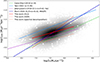 |
Fig. 5. Results of the rSFMS compared to other works. The gray hexagonal bins depict the distribution of our data points, estimated via Gaussian kernels, where darker bins correspond to a higher density of data points. The solid red line represents our results using an ordinary least square (OLS) fitting and the dotted red line is for an orthogonal distance regression (ODR). The solid blue line is the result of Yao et al. (2022) at z ∼ 0.26, and the solid purple line is of Jafariyazani et al. (2019) at 0.1 < z < 0.42, both of which cover a similar redshift range to ours. The dashed green line comes from Cano-Díaz et al. (2016) for the local Universe. As a comparison, we also present our results via OLS when applying the spectral decomposition method from Davies et al. (2017) (see Sect. 4.1.2) as a pink line. The gray errorbar shows the average uncertainties in ΣSFR and Σ*. FADO only gives errors based on the goodness of the fit, stellar mass errors are very small, and the average Σ* is not visible within this plot. |
Using EAGLE hydrodynamical cosmological simulations, Trayford & Schaye (2019), predict that the slope of the rSFMS increases with increasing redshift, which they attribute to inside-out galaxy formation. Table 1 lists our results and those from several other publications, showing that our resulting OLS slope diverges from the expected trend in rSFMS slope evolution with redshift. In Table 1 we also list each publication’s utilized data range and fitting routine method. However, the OLS slope aligns well with the results obtained from Jafariyazani et al. (2019), who utilized MUSE data at 0.1 < z < 0.42 but for lower stellar masses. Nonetheless, our relatively shallow OLS rSFMS slope might result from MAGPI fields often probing dense environments, which are more prone to phenomena suppressing star formation such as environmental quenching (see e.g., Mao et al. 2022; Taylor et al. 2023). On the other hand, Popesso et al. (2022) recently conducted a study of the SFMS redshift evolution, where they compiled existing studies of the SFMS over a total redshift range of 0 < z < 6 and stellar mass of 8.5 < log(M*/M⊙) < 11.5. They find that only the normalization and turnover mass evolve over time, but not the slope.
Best-fit values of the rSFMS for our work and several other publications.
We also applied an ODR fitting routine, as shown in Table 1, and the resulting slope aligns much better with the expected redshift evolution. Hsieh et al. (2017) also analyzed the rSFMS using both an OLS and ODR fitting routine. They find that a steeper slope is measured via the ODR method. Comparing our ODR slope to that of Hsieh et al. (2017), we can detect a redshift evolution.
The SFR values for our sample match those from Jafariyazani et al. (2019) and are mainly located above the local Universe’s SFRs from Cano-Díaz et al. (2016). This result agrees with the observations that galaxies at higher redshifts have higher SFRs than in the local Universe. Nonetheless, we observe lower SFRs than Yao et al. (2022) who conducted a similar analysis using MUSE data at a redshift of z ∼ 0.26. We conclude that this could be caused by the differences in the selection and depth of the data used and the S/N criteria applied to select spaxels.
Mun et al. (2024) also investigate the rSFMS via MAGPI data using a least trimmed squares (LTS) routine and find a slope of 0.922, which aligns more with the findings of the redshift evolution than our OLS slope. Comparing their LTS results to our ODR slope, we are in relatively good agreement. Their results are also plotted as a dark-blue line in Fig. 5. However, their analysis was conducted within a redshift range of 0.25 < z < 0.42 and a much wider total stellar mass range, including low-mass galaxies within 6.2 ≲ log(M*/M⊙)≲11.4. As we need sufficient S/N in all four emission lines [OIII]5006 Å, Hβ, Hα, and [NII]6585 Å, and therefore applied an S/N cut when selecting our sample, our sample size is much smaller in comparison. The wider mass range could explain their higher completeness within the low-Σ* and low-ΣSFR section of the log Σ* versus log ΣSFR distribution compared to our analysis.
We repeated the same analysis of the rSFMS by applying the spectral decomposition method introduced in Sect. 4.1.2 to all spaxels present in the BPT diagram and show the result as a pink-colored line in Fig. 5. For this, we computed the fractional contribution of SF, AGN, and LINER to the Hα emission line and corrected our Hα fluxes to only consist of its SF contribution. This method aims to have a larger sample available for investigating the rSFMS, as our normal attempts consist of filtering out any spaxels that fall above the empirical line from Kauffmann et al. (2003), which inherently limits our sample. The resulting OLS rSFMS has the following parameters: a = −5.359 ± 0.082 and b = 0.368 ± 0.011. Additionally, we repeated an ODR analysis and find the following results: a = −22.248 ± 0.431 and b = 2.562 ± 0.056. The OLS slope of this result is consistent with the OLS slope for SF spaxels, but the SFRs are located below the results for SF spaxels. We consider the difference in the zero-point of our two fits to stem from the fact that there are more low log(ΣSFR) spaxels via the spectral decomposition method compared to only selecting SF-spaxels.
4.4. Resolved MZR
Figure 6 shows the distribution of the gas-phase metallicity for star-forming spaxels as a function of their stellar mass surface density. The gray hexagonal bins represent our star-forming spaxels. As the surface mass density increases, the oxygen abundances also increase. As noted by previous studies (see e.g., Tremonti et al. 2004; Zahid et al. 2013), the relation flattens toward higher stellar masses. The average uncertainty of the gas-phase metallicity is ∼0.08 dex. Within a mass range of 6.87 ≲ log Σ∗ (M⊙ kpc−2) ≲ 8.33, which is defined as the range that covers 80% of the data, we performed a nonlinear least square fit via the following equation from Sánchez et al. (2013):
 (7)
(7)
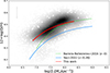 |
Fig. 6. Distribution of the gas-phase metallicities of our sample of star-forming spaxels against their stellar mass surface densities. The hexagonal bins depict the sample distribution with darker colors corresponding to a denser region of data points. The corresponding fitting result for our data within a mass range of 6.87 ≲ log Σ∗ (M⊙ kpc−2) ≲ 8.33, which is defined as the range that covers 80% of the data, was computed via Eq. (7) from Sánchez et al. (2013) and is shown as a red line. The gray errorbar in the top left corner shows the average uncertainties in gas-phase metallicity and Σ*. FADO only gives errors based on the goodness of the fit, stellar mass errors are very small, and the average Σ* is not visible within this plot. |
The results from our fitting routine for the coefficients are a = 8.561 ± 0.016, b = 0.0001 ± 0.0006, and c = 12.7 ± 5.542. We obtain a 1σ scatter, derived by calculating the standard deviation of the residual between the observed and fitted gas-phase metallicity, of 0.08 dex.
We compare our results to the results obtained by Barrera-Ballesteros et al. (2016) for the local Universe utilizing 653 galaxies from the MaNGA survey covering a total stellar mass range of 8.5 ≲ log(M*/M⊙)≲11 and those by Yao et al. (2022) at a similar average redshift of z ∼ 0.26 over a mass range of 9 ≲ log(M*/M⊙)≲10.6 using the MUSE wide survey. Barrera-Ballesteros et al. (2016) also applied the same strong-line metallicity calibration by Marino et al. (2013) from Te-based HII regions, and differences in the IMF are accounted for. Yao et al. (2022) utilized metallicity calibration from ONS-based HII regions by Marino et al. (2013) and we have adjusted for the difference between their ONS-based and our Te-based calibrations. Results by Yao et al. (2022) are of a similar shape, but their metallicities are below ours, with an average downward shift of ∼0.09 dex. This could be explained by their overall smaller sample, which also covers a smaller total mass range, whereas in our case, about a third of our sample exhibits log(M*/M⊙) > 10.6, leading to our sample being more metal-rich. We, therefore, investigated whether our sample’s M* range might affect our resulting oxygen abundances. We created a subset of galaxies within our sample that matches the mass range 9 ≲ log(M*/M⊙)≲10.6 from Yao et al. (2022). Still, the resulting rMZR fit is on average at only 0.009 dex lower than our entire sample. Thus, we cannot confirm that the differences in our gas-phase metallicities from those by Yao et al. (2022) stem from any difference in the sample’s total stellar mass range.
Gas-phase metallicities are observed to evolve with redshift: for a given stellar mass, metallicity declines with increasing redshift. This evolution is strongly defined within low-mass galaxies, while high-mass galaxies are believed to have already reached their local metallicity values at z ∼ 1 due to downsizing (Maiolino & Mannucci 2019). Barrera-Ballesteros et al. (2016) results of the rMZR for the local Universe are situated below those of ours, with a ∼0.03 dex downward shift, which again confirms the overall high metallicities within our sample. Therefore, we do not observe any redshift evolution of the rMZR. On the other hand, Barrera-Ballesteros et al. (2016) results are significantly above those obtained by Yao et al. (2022) at z ∼ 0.26, with the former aligning more reasonably with the expected metallicity redshift evolution. Furthermore, as mentioned in Sect. 4.2.2, Maier et al. (2015) found that there is only a low offset between the gas-phase metallicities at z = 0 and at 0.5 < z < 0.75. Assuming similarity in the resolved version, we expect only a small offset between our sample at z = 0.3 and the local Universe.
Lastly, we conducted a simple environmental analysis of the gas-phase metallicities within our sample. Gas-phase metallicities have consistently been observed to be higher in dense environments than in field galaxies (see e.g., Cooper et al. 2008), which could explain why our values for MAGPI galaxies, which lie mostly within dense environments, are similar to those for the local Universe. To investigate this, we separated MAGPI’s primary groups from field galaxies by considering the following selection: |zsecondary − zprimary|< 0.03. Here, zprimary are redshifts of MAGPI’s group galaxies, while zsecondary are redshifts of secondary galaxies within the same field as its corresponding primary galaxy. Galaxies with a redshift difference lower than 0.03 are considered part of the primary group. We find that group galaxies have consistently higher gas-phase metallicities than field galaxies, averaging about 0.02 dex. Also, the resulting rMZR fit for group galaxies is, on average, 0.01 dex higher than for field galaxies. This is consistent with results from other works such as Geha et al. (2024) which investigated the environmental processes of star-forming properties of 378 satellite galaxies in the local Universe from the Satellites Around Galactic Analogs (SAGA; Geha et al. 2017) survey and Maier et al. (2022) who studied 18 clusters from the Local Cluster Substructure Survey (LoCuSS; Smith et al. 2010) at z ∼ 0.2.
4.5. Resolved FMR
To produce quantitative statistical results for our analysis of the spatially resolved FMR, we make use of a partial correlation coefficient (PCC) analysis similar to the one presented by Baker et al. (2021, 2022). The analysis involves determining the partial correlation between two variables while keeping other variables constant. This approach helps us discern the genuine and inherent correlations between the two variables, distinguishing them from indirect correlations arising from other scaling relationships. In this sense, an equation can be defined where the partial correlation between two variables, A and B, is tested while controlling for a third variable, C:
 (8)
(8)
Here, ρXY refers to the Spearman rank correlation coefficient between two variables X and Y. It is important to note that PCCs will only give meaningful results for monotonic relations. In the case of our analysis, it is helpful to picture the dependence of the three variables as a 3D space where the points on B (y-axis) are plotted versus C (x-axis) and color-coded by A (z-axis). In this sense, gas-phase metallicities are our variable A, ΣSFR is B, and Σ* is C. Another useful way to quantify PCC results is to produce an arrow pointing toward the steepest average gradient of increase of the variable A, in this case, the metallicity, therefore allowing us to determine the role of B and C, ΣSFR and Σ*, in driving the gas-phase metallicity A. The angle Θ of this arrow is measured from the horizontal (three o’clock position) and is defined by the following equation from Bluck et al. (2020):
 (9)
(9)
Thus, this arrow angle is derived by taking the ratio of the PCC, looking at the influence of ΣSFR on the metallicity while controlling for Σ* and the PCC determining the influence of Σ* on the metallicity while controlling for ΣSFR. To obtain arrow angle uncertainties, we applied the same method as Baker et al. (2022) and utilized bootstrap random sampling to 100 random samples of the data and compute their standard deviation.
Figure 7 shows log(ΣSFR) versus log(Σ*), color-coding our data points with the local gas-phase metallicity 12 + log(O/H) and including the arrow angle as defined in Eq. (9) in the top left corner of each Figure. This figure is smoothed using LOESS, a Python package that applies a locally weighted regression method to obtain mean trends of noisy data (Cappellari et al. 2013). The stronger the arrow points vertically, the stronger the influence of ΣSFR on driving the local metallicities. Similarly, the more horizontal the arrow appears, the stronger the influence of Σ* in determining the local gas-phase metallicity.
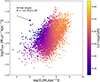 |
Fig. 7. Resolved fundamental metallicity relation for the star-forming spaxels of our sample. Here, log(Σ*) is plotted against log(ΣSFR) and each spaxel is color-coded by its gas-phase metallicity 12 + log(O/H). Additionally, an arrow angle and its error point to the direction of the steepest average gradient of increase of the local metallicity. Images are smoothed over via LOESS (Cappellari et al. 2013), a locally weighted regression method to compute mean trends of the population from noisy data. |
The color shading alone demonstrates how ΣSFR and Σ* drive the local metallicity. If only Σ* influenced the metallicity, there would be vertical gradients of color as the metallicity would not change with ΣSFR at all. On the contrary, if only ΣSFR determined the metallicity, we would expect results of horizontal gradients of color. In our case, we see a color shading that indicates that the metallicity is proportionally correlated with Σ* and inversely correlated with ΣSFR. The direction of the color shading also indicates that Σ* is the dominant factor in determining the metallicity.
We look at the arrow angle depicted in Fig. 7 to better understand these correlations. For our sample, we obtain a result of Θ = −12.43 ± 1.25°. This corresponds to a 13.81% contribution from ΣSFR and 86.19% contribution from Σ* to the spatially resolved gas-phase metallicity. The direction in which the arrow angle points indicates that Σ* has a stronger correlation with the gas-phase metallicity than ΣSFR does, but that both combined determine the metallicity. In conclusion, there is a small but significant contribution from ΣSFR in driving the local metallicity, although Σ* remains the dominant influence. Therefore, to increase the metallicity, an increase in Σ* is needed, which is what would be expected from the rMZR. Still, a secondary inverse dependence exists on ΣSFR for the metallicity. An increase in ΣSFR weakly correlates with a decrease in the local metallicity. Our ratio is much smaller than the one reported by Baker et al. (2022) of Θ = −40° for their entire sample of local galaxies covering stellar masses of 9.0 < log(M*/M⊙) < 11.4.
We repeated our analysis of the arrow angle by grouping our data into different bins of total stellar mass. The results are summarized in Table 2. In conclusion, galaxies at the lower-mass end of our sample show a significantly stronger contribution of ΣSFR on the metallicity than higher-mass galaxies. Baker et al. (2022) also repeated their analysis by grouping their data into three separate mass bins, with their highest mass bin of 10.6 < log(M*/M⊙) < 11.4 resulting in an arrow angle of −16.6° and, therefore, they report a ratio of 18.44% ΣSFR and 81.56% Σ* contribution. Hence, their highest mass bin arrow angle aligns the most with our results. Generally, their results indicate a stronger influence of ΣSFR on the metallicity in the local Universe than our overall results indicate at z ∼ 0.3.
Figure 8 shows the rMZR binned by ΣSFR, similar to the FMR analysis done by Mannucci et al. (2010), and is a different way to visualize the rFMR. Here, the different colored tracks correspond to the rMZR fits done via Eq. (7) for different log(ΣSFR) bins, as described in the legend, while the dashed red line is the rMZR fit derived in Sect. 3.3 covering the entire sample. There were substantial outliers toward lower stellar mass surface densities, so the different bins are plotted within a log(Σ*) range that covers 80% of the data. Figure 8 further supports the existence of an rFMR for lower Σ*. At roughly log(Σ*)∼7.8, the inverse correlation between gas-phase metallicity and SFR flattens out and even seemingly inverts to a certain degree. At any point below log(Σ*)∼8, we find that for a fixed Σ*, higher ΣSFR correlate with lower 12 + log(O/H).
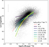 |
Fig. 8. Resolved mass-metallicity relation for different ΣSFR bins, as indicated in the legend. Each line represents a rMZR fit for the different corresponding ΣSFR bins computed as described in Sect. 4.4. The dashed red line represents the results for all SF spaxels following Eq. (7). The gray errorbar shows the average uncertainties in gas-phase metallicity and Σ*. FADO only gives errors based on the goodness of the fit, stellar mass errors are very small, and the average Σ* is not visible within this plot. |
4.6. Local metallicity dependence on resolved and global properties
To get a deeper look at the strengths of the relations defining the local metallicity, we computed the partial correlation coefficients between the resolved metallicity and Σ*, M*, ΣSFR, and SFR while controlling for either Σ* (when analyzing the correlation with M*), M* (when analyzing the correlation with Σ*), or both (when analyzing the correlation with ΣSFR and SFR).
Results are shown as a bar chart in Fig. 9 with error bars indicating the uncertainties obtained via bootstrap random sampling. A uniform random variable was also included as a control mechanism. This analysis provides us with the strength and sign of the correlations, although it should be mentioned again that PCCs only work accurately for monotonic relations. The local stellar mass density Σ* is the main driver of the local metallicity, followed by the total stellar mass M*. The total SFR and ΣSFR show only a weak correlation, with the total SFR even positively correlating with the local metallicity. The strength at which ΣSFR negatively correlates with the gas-phase metallicity is also much weaker than the results from Baker et al. (2022) for the local Universe.
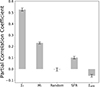 |
Fig. 9. Partial correlation coefficients of the local metallicity and the resolved stellar mass surface density Σ*, total stellar mass M*, a uniform random variable, resolved star formation rate ΣSFR, and total star formation rate SFR. Errors shown as error bars are computed via bootstrap random sampling. |
We note that Baker et al. (2022) also employed a random forest algorithm to determine the relative importance of each parameter on the metallicity, which has better accuracy in determining their true correlations than the Partial Correlation Coefficient analysis does. What is important to conclude from these results is that Σ* is evidently the dominating influence on the local metallicity, followed by total stellar mass M*. Suppose the partial correlation coefficient analysis should only be taken at face value regarding the sign of the correlations and not at their correlation strength. In that case, these results indicate an anti-correlation between ΣSFR and 12 + log(O/H).
To give another way to quantify our results of the rFMR, we investigated the relation between the gas-phase metallicity and the parameter μα, which was first defined by Mannucci et al. (2010):
 (10)
(10)
This function is defined to parametrize the projection of the FMR that minimizes the scatter in metallicity. Therefore, α = 0 would correspond to μ0 = log(M*), while α = 1 would result in μ1 = −log(sSFR). Their argument for this type of parametrization is that the value of α that minimizes the scatter of the median metallicities around the relation corresponds to a μα that exhibits the tightest possible, “most fundamental” correlation with the gas-phase metallicity.
Here, the function μα is minimized to find the value of α that minimizes the dispersion between 12 + log(O/H) and μα. For our sample, we find α = 0.42 for SF spaxels with an average dispersion of around ∼0.09 dex, around ∼0.17 dex lower than the average dispersion for α = 0, confirming the existence of an rFMR. We plot the dispersion as a function of α in Fig. 10 and indicate our minimum dispersion as a dashed red line. Our reported α parameters also align well with the initial finding of α = 0.32 by Mannucci et al. (2010), which results in an average dispersion that is only 0.02 dex higher than that of our optimal α. Other investigations into the spatially resolved 12 + logO/H versus μα relation have resulted in various values: Baker et al. (2022) (α = 0.54, z ∼ 0), Li et al. (2024) (α = 0.33, 0.01 ≲ z ≲ 0.15), Andrews & Martini (2013) (α = 0.66, 0.027 < z < 0.25), and Yao et al. (2022) (α = 0.51, z ∼ 0.26).
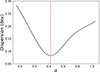 |
Fig. 10. Residual dispersion of the gas-phase metallicities as a function of α following Eq. (10). The value of α = 0.42, corresponding to the minimum dispersion, is highlighted as a dashed red line. |
4.7. Voronoi binning
We also repeated our entire analysis via Voronoi binning (Vorbin; Cappellari & Copin 2003), binning our spaxel data to ensure a high enough S/N of the emission lines for our spatially resolved analysis of gas-phase metallicities. This method relies on Voronoi tessellations to bin spectral data to a minimum S/N requirement.
Vorbin needs a target S/N value for each spaxel. We computed the S/N within an observed wavelength window of 6050 Å < λobs < 7750 Å, corresponding roughly to the peak MUSE sensitivity range, and set the minimum target S/N to 8. Only spaxels with a minimum S/N of 2 were included in the binning process. All spectra in one bin were stacked and averaged. We applied the same steps regarding extinction correction and emission line flux measurements as described in Sect. 3. To conclude, we do not find significant differences between our results via a spaxel-by-spaxel analysis and Voronoi binning.
5. Discussion
Our main goal is to determine the interdependence between the spatially resolved and global parameters defining the rFMR. We find that for our sample, the local gas-phase metallicity primarily correlates with Σ* and has an inverse secondary correlation with ΣSFR, as can be seen per Figs. 7 and 8, confirming an rFMR at z ∼ 0.3. This aligns well with the theory that the FMR is caused by the accretion of pristine metal-poor gas, which both dilutes the overall gas content in a galaxy, decreasing its metallicity and increases the overall SFR as it acts as a star formation boost (see e.g., Tremonti et al. 2004; Mannucci et al. 2010; Lara-López et al. 2010; Lilly et al. 2013). However, the fact that the global SFR has a stronger and, more importantly, positive correlation with the local gas-phase metallicity majorly diverges from this theory. These results also greatly contrast what Baker et al. (2022) find using the same partial correlation coefficient analysis for the local Universe, where their inverse correlation with both SFR and ΣSFR underlines the necessity of both the accretion-dilution scenario that is typically associated with the FMR and the need for metal-rich galactic-scale outflows caused by winds.
When analyzing the rFMR, we only find a weak correlation between the local metallicity and ΣSFR as indicated by the arrow angle. Our angle of −12.43° corresponds to a roughly 14% contribution from ΣSFR and 86% contribution from Σ* to the spatially resolved metallicity. However, when investigating these interdependences in more detail, we notice a significant turnover at log(Σ*)≳7.8, where the rFMR starts to weaken and even inverts. This is best depicted in Fig. 8 where we plotted and fitted the rMZR for different ΣSFR bins. Similarly, Baker et al. (2022) investigated the rFMR by plotting the metallicity versus Σ* binned by tracks of different ΣSFR and observed a similar inversion at high Σ*. Furthermore, we also tested how well the rFMR is defined for a log(Σ*) < 7.8. We find that it produces an arrow angle of ∼ − 27.3 ± 1.5°, which indicates a stronger inverse influence of ΣSFR on the local metallicity than when considering our full Σ* range.
In Sect. 4.4 we investigated whether our differences in rMZR between our sample and those by Yao et al. (2022), who also utilized MUSE data at a similar redshift of z ∼ 0.26 but for a smaller stellar mass range of 9 ≲ log(M*/M⊙)≲10.6, could be explained by the influence of M* on the rMZR. To conclude, we created a subsample of our data that matches the mass range of Yao et al. (2022) and re-fitted the rMZR. The resulting fit is located only minimally below that for our entire sample, and we can not explain this difference via a dependence on M*. However, as mentioned in Sect. 6, a difference in the exposure times of the observations between the MUSE-wide survey utilized by Yao et al. (2022), which has a total integration time of 1 h and our MAGPI data with an exposure time of 4.4 h per field, could possibly explain their overall higher SFRs and lower gas-phase metallicities compared to ours.
Nevertheless, we note that a cut in Σ*, as discussed above, is similar to a cut in M*, as is indicated by the arrow angle results shown in Table 2 for different M* bins. Therefore, we find evidence of a significant influence of M* on the gas-phase metallicity via the partial correlation coefficients and arrow angle analysis. In fact, the correlation between M* and the local metallicity is stronger than between the metallicity and ΣSFR. Only selecting low Σ* spaxels or low M* galaxies results in a stronger contribution from SFR to the spatially resolved metallicity. We also observe that the highest Σ* spaxels stem from our highest M* galaxies. Hence, we find good evidence for an rFMR at z ∼ 0.31 for selecting spaxels with log(Σ*)≲7.8 or galaxies with log(M*/M⊙)≲10.6. Beyond those, the relation starts to flatten out and even invert. Hence, the overall small contribution from ΣSFR toward the local metallicity for our entire sample could also be explained by our sample’s bias toward higher M*.
Bulichi et al. (2023), who analyzed the rFMR for nine local dwarf galaxies via MUSE data, also concluded that the anti-correlation between gas-phase metallicity and ΣSFR is strongest for low-mass galaxies. This is also confirmed by the results from Curti et al. (2019). The fact that the FMR is most pronounced toward low-mass galaxies aligns well with our results and has even been replicated via EAGLE simulations (Scholz-Díaz et al. 2021). This also follows expectations that SN feedback, which is responsible for metal supply, mixing, and ejection of metal-rich material and dilution effects caused by a strong inflow of metal-poor gas, are most prominent in low-mass galaxies. Mannucci et al. (2010) argued that the outflow of gas is responsible for the metallicity’s dependence on stellar mass, as winds are more efficient in carrying out metals inside lower-mass galaxies and that toward higher-mass galaxies, the efficiency of outflows decreases due to the galaxies larger potential wells. Therefore, both effects can decrease gas-phase metallicities in low-mass galaxies and fuel their star formation. Indeed, observations have shown that SN feedback-driven outflows exhibit higher gas-phase metallicities than the ISM of its origin galaxy (Chisholm et al. 2018). On the other hand, AGN feedback starts to dominate galactic outflows in high-mass galaxies, which are generally better at retaining metals due to their deeper gravitational potential, thus decreasing the impact of ΣSFR on the local metallicity at higher M*.
6. Summary and conclusion
We utilized data from the MUSE Large Program MAGPI. We selected 65 galaxies with strong optical emission lines over a redshift range of 0.28 < z < 0.35 and within a total stellar mass range of 8.2 < log(M*/M⊙) < 11.4. We measured emission line fluxes and stellar masses via the population spectral synthesis code FADO to reliably determine the galaxies ΣSFR, Σ*, and spatially resolved gas-phase metallicities.
Our main results are as follows:
-
Via diagnostic diagrams, we confirm that the main ionizing mechanism in our sample is SF and that the empirical and theoretical line calibrations used to distinguish between the different ionizing mechanisms align well with the fractional contribution of SF, AGN, and LINER emission, computed via the spectral decomposition method from Davies et al. (2017), to the Hα line.
-
We establish a global SFMS and MZR for our sample. The SFMS aligns well with the results found in other works. Our sample exhibits overall high gas-phase metallicities, as they are within the relation found for the local Universe.
-
We confirm the existence of an rSFMS at z ∼ 0.3 with a slope of ∼0.425. This resulting slope is shallower than expected if a redshift evolution of the slope is assumed. However, via ODR fitting, we find a slope of ∼1.162, which aligns better with the expected redshift evolution. Our spatially resolved SFRs are higher than those observed for the local Universe, which aligns with the theory that galaxies exhibit increasing SFRs toward higher redshifts. We find similar rSFMR slopes for our fits obtained by only selecting SF-spaxel, and when using the Hα emission line, corrected to only include its SF contribution via the spectral decomposition method.
-
The rMZR exists at z ∼ 0.3, but we find overall high gas-phase metallicities which are on average 0.03 dex higher than the local Universe’s values, which is still within the diagnostic’s uncertainty. This is also confirmed by our global MZR shown in Fig. 4, where our galaxies are observed to be within the local relation.
-
We tentatively confirm the existence of an rFMR: the spatially resolved gas-phase metallicity primarily depends on the local stellar mass surface density Σ* with a secondary, inverse, dependence on the local star formation rate surface density ΣSFR.
-
We investigated the correlation between global and resolved parameters through a partial correlation coefficient analysis. The two dominant factors in determining the local metallicity are Σ* and M*, albeit, Σ* has a significantly higher contribution than M*. Additionally, ΣSFR weakly inversely correlates with the local metallicity. We observe that the inverse correlation between the spatially resolved metallicity and ΣSFR significantly strengthens toward lower M* and Σ*.
Based on observations obtained at the Very Large Telescope (VLT) of the European Southern Observatory (ESO), Paranal, Chile (ESO program ID 1104.B-0536).
Acknowledgments
We wish to thank the ESO staff, and in particular the staff at Paranal Observatory, for carrying out the MAGPI observations. MAGPI targets were selected from GAMA. GAMA is a joint European-Australasian project based around a spectroscopic campaign using the Anglo-Australian Telescope. GAMA was funded by the STFC (UK), the ARC (Australia), the AAO, and the participating institutions. GAMA photometry is based on observations made with ESO Telescopes at the La Silla Paranal Observatory under programme ID 179.A-2004, ID 177.A-3016. The MAGPI team acknowledge support by the Australian Research Council Centre of Excellence for All Sky Astrophysics in 3 Dimensions (ASTRO 3D), through project number CE170100013. CF is the recipient of an Australian Research Council Future Fellowship (project number FT210100168) funded by the Australian Government. CL, JTM and CF are the recipients of ARC Discovery Project DP210101945. SMS acknowledges funding from the Australian Research Council (DE220100003). LMV acknowledges support by the German Academic Scholarship Foundation (Studienstiftung des deutschen Volkes) and the Marianne-Plehn-Program of the Elite Network of Bavaria. KG is supported by the Australian Research Council through the Discovery Early Career Researcher Award (DECRA) Fellowship (project number DE220100766) funded by the Australian Government. PP acknowledges support by the Fundação para a Ciência e a Tecnologia (FCT) grants UID/FIS/04434/2019, UIDB/04434/2020, UIDP/04434/2020 and Principal Investigator contract CIAAUP-092023-CTTI This work uses the following software packages: Astropy (Astropy Collaboration 2013), FADO (Gomes & Papaderos 2017), GIST (Bittner et al. 2019), lmfit (Newville et al. 2016), LOESS (Cappellari et al. 2013), Matplotlib (Hunter 2007), MPDAF (Bacon et al. 2016), Numpy (Harris et al. 2020), Pingouin (Vallat 2018), Profound (Robotham et al. 2018), Prospect (Robotham et al. 2020), Scipy (Virtanen et al. 2020), Seaborn (Waskom 2021), Uncertainties (https://pythonhosted.org/uncertainties/), and Vorbin (Cappellari & Copin 2003).
References
- Andrews, B. H., & Martini, P. 2013, ApJ, 765, 140 [NASA ADS] [CrossRef] [Google Scholar]
- Astropy Collaboration (Price-Whelan, A. M., et al.) ApJ, 935, 167 [Google Scholar]
- Bacon, R., Piqueras, L., Conseil, S., Richard, J., & Shepherd, M. 2016, Astrophysics Source Code Library [record ascl:1611.003] [Google Scholar]
- Baker, W. M., Maiolino, R., Bluck, A. F. L., et al. 2021, MNRAS, 510, 3622 [Google Scholar]
- Baker, W. M., Maiolino, R., Belfiore, F., et al. 2022, MNRAS, 519, 1149 [NASA ADS] [CrossRef] [Google Scholar]
- Baldwin, J. A., Phillips, M. M., & Terlevich, R. 1981, PASP, 93, 5 [Google Scholar]
- Barrera-Ballesteros, J. K., Heckman, T. M., Zhu, G. B., et al. 2016, MNRAS, 463, 2513 [NASA ADS] [CrossRef] [Google Scholar]
- Bittner, A., Falcón-Barroso, J., Nedelchev, B., et al. 2019, A&A, 628, A117 [NASA ADS] [CrossRef] [EDP Sciences] [Google Scholar]
- Bluck, A. F. L., Maiolino, R., Piotrowska, J. M., et al. 2020, MNRAS, 499, 230 [NASA ADS] [CrossRef] [Google Scholar]
- Boogaard, L. A., Brinchmann, J., Bouché, N., et al. 2018, A&A, 619, A27 [NASA ADS] [CrossRef] [EDP Sciences] [Google Scholar]
- Brinchmann, J., Charlot, S., White, S. D. M., et al. 2004, MNRAS, 351, 1151 [Google Scholar]
- Bruzual, G., & Charlot, S. 2003, MNRAS, 344, 1000 [NASA ADS] [CrossRef] [Google Scholar]
- Bulichi, T.-E., Fahrion, K., Mernier, F., et al. 2023, A&A, 679, A98 [NASA ADS] [CrossRef] [EDP Sciences] [Google Scholar]
- Bundy, K., Bershady, M. A., Law, D. R., et al. 2015, ApJ, 798, 7 [Google Scholar]
- Calzetti, D. 2001, PASP, 113, 1449 [Google Scholar]
- Cano-Díaz, M., Sánchez, S. F., Zibetti, S., et al. 2016, ApJ, 821, L26 [Google Scholar]
- Cappellari, M. 2017, MNRAS, 466, 798 [Google Scholar]
- Cappellari, M., & Copin, Y. 2003, MNRAS, 342, 345 [Google Scholar]
- Cappellari, M., & Emsellem, E. 2004, PASP, 116, 138 [Google Scholar]
- Cappellari, M., McDermid, R. M., Alatalo, K., et al. 2013, MNRAS, 432, 1862 [NASA ADS] [CrossRef] [Google Scholar]
- Cardelli, J. A., Clayton, G. C., & Mathis, J. S. 1989, ApJ, 345, 245 [Google Scholar]
- Chabrier, G. 2003, PASP, 115, 763 [Google Scholar]
- Chisholm, J., Tremonti, C., & Leitherer, C. 2018, MNRAS, 481, 1690 [NASA ADS] [CrossRef] [Google Scholar]
- Cooper, M. C., Tremonti, C. A., Newman, J. A., & Zabludoff, A. I. 2008, MNRAS, 390, 245 [NASA ADS] [CrossRef] [Google Scholar]
- Cresci, G., Mannucci, F., Sommariva, V., et al. 2012, MNRAS, 421, 262 [NASA ADS] [Google Scholar]
- Cresci, G., Mannucci, F., & Curti, M. 2019, A&A, 627, A42 [NASA ADS] [CrossRef] [EDP Sciences] [Google Scholar]
- Croom, S. M., Owers, M. S., Scott, N., et al. 2021, MNRAS, 505, 991 [NASA ADS] [CrossRef] [Google Scholar]
- Curti, M., Mannucci, F., Cresci, G., & Maiolino, R. 2019, MNRAS, 491, 944 [Google Scholar]
- Curti, M., D’Eugenio, F., Carniani, S., et al. 2022, MNRAS, 518, 425 [CrossRef] [Google Scholar]
- Curti, M., Maiolino, R., Curtis-Lake, E., et al. 2024, A&A, 684, A75 [NASA ADS] [CrossRef] [EDP Sciences] [Google Scholar]
- Davies, R. L., Groves, B., Kewley, L. J., et al. 2016, MNRAS, 462, 1616 [NASA ADS] [CrossRef] [Google Scholar]
- Davies, R. L., Groves, B., Kewley, L. J., et al. 2017, MNRAS, 470, 4974 [NASA ADS] [CrossRef] [Google Scholar]
- Driver, S. P., Hill, D. T., Kelvin, L. S., et al. 2011, MNRAS, 413, 971 [Google Scholar]
- Driver, S. P., Robotham, A. S. G., Bland-Hawthorn, J., et al. 2013, MNRAS, 430, 2622 [NASA ADS] [CrossRef] [Google Scholar]
- Ellison, S. L., Patton, D. R., Simard, L., & McConnachie, A. W. 2008, ApJ, 672, L107 [NASA ADS] [CrossRef] [Google Scholar]
- Ellison, S. L., Sánchez, S. F., Ibarra-Medel, H., et al. 2018, MNRAS, 474, 2039 [Google Scholar]
- Foster, C., Mendel, J. T., Lagos, C. D. P., et al. 2021, PASA, 38, e031 [NASA ADS] [CrossRef] [Google Scholar]
- Gao, Y., Bao, M., Yuan, Q., et al. 2018, ApJ, 869, 15 [NASA ADS] [CrossRef] [Google Scholar]
- Garcia, A. M., Torrey, P., Ellison, S., et al. 2024, MNRAS, 531, 1398 [NASA ADS] [CrossRef] [Google Scholar]
- Geha, M., Wechsler, R. H., Mao, Y.-Y., et al. 2017, ApJ, 847, 4 [NASA ADS] [CrossRef] [Google Scholar]
- Geha, M., Mao, Y. Y., Wechsler, R. H., et al. 2024, ApJ, accepted [arXiv:2404.14499] [Google Scholar]
- Gomes, J. M., & Papaderos, P. 2017, A&A, 603, A63 [NASA ADS] [CrossRef] [EDP Sciences] [Google Scholar]
- Harris, C. R., Millman, K. J., van der Walt, S. J., et al. 2020, Nature, 585, 357 [NASA ADS] [CrossRef] [Google Scholar]
- Hinton, S. R., Davis, T. M., Lidman, C., Glazebrook, K., & Lewis, G. F. 2016, Astron. Comput., 15, 61 [Google Scholar]
- Hsieh, B. C., Lin, L., Lin, J. H., et al. 2017, ApJ, 851, L24 [Google Scholar]
- Hunter, J. D. 2007, Comput. Sci. Eng., 9, 90 [NASA ADS] [CrossRef] [Google Scholar]
- Jafariyazani, M., Mobasher, B., Hemmati, S., et al. 2019, ApJ, 887, 204 [NASA ADS] [CrossRef] [Google Scholar]
- Kauffmann, G., Heckman, T. M., Tremonti, C., et al. 2003, MNRAS, 346, 1055 [Google Scholar]
- Kennicutt, R. C., Jr. 1998, ARA&A, 36, 189 [Google Scholar]
- Kewley, L. J., & Ellison, S. L. 2008, ApJ, 681, 1183 [Google Scholar]
- Kewley, L. J., Dopita, M. A., Sutherland, R. S., Heisler, C. A., & Trevena, J. 2001, ApJ, 556, 121 [Google Scholar]
- Kewley, L. J., Nicholls, D. C., & Sutherland, R. S. 2019, ARA&A, 57, 511 [Google Scholar]
- Kollmeier, J., Anderson, S. F., Blanc, G. A., et al. 2019, BAAS, 51, 274 [NASA ADS] [Google Scholar]
- Lamareille, F. 2010, A&A, 509, A53 [CrossRef] [EDP Sciences] [Google Scholar]
- Lamareille, F., Brinchmann, J., Contini, T., et al. 2009, A&A, 495, 53 [NASA ADS] [CrossRef] [EDP Sciences] [Google Scholar]
- Lara-López, M. A., Cepa, J., Bongiovanni, A., et al. 2010, A&A, 521, L53 [CrossRef] [EDP Sciences] [Google Scholar]
- Lequeux, J., Peimbert, M., Rayo, J. F., Serrano, A., & Torres-Peimbert, S. 1979, A&A, 80, 155 [Google Scholar]
- Leslie, S. K., Schinnerer, E., Liu, D., et al. 2020, ApJ, 899, 58 [Google Scholar]
- Li, S.-L., Grasha, K., Krumholz, M. R., et al. 2024, MNRAS, 529, 4993 [NASA ADS] [CrossRef] [Google Scholar]
- Lilly, S. J., Fèvre, O. L., Renzini, A., et al. 2007, ApJS, 172, 70 [NASA ADS] [CrossRef] [Google Scholar]
- Lilly, S. J., Carollo, C. M., Pipino, A., Renzini, A., & Peng, Y. 2013, ApJ, 772, 119 [NASA ADS] [CrossRef] [Google Scholar]
- Madau, P., & Dickinson, M. 2014, ARA&A, 52, 415 [Google Scholar]
- Maier, C., Lilly, S. J., Ziegler, B. L., et al. 2014, ApJ, 792, 3 [NASA ADS] [CrossRef] [Google Scholar]
- Maier, C., Ziegler, B. L., Lilly, S. J., et al. 2015, A&A, 577, A14 [NASA ADS] [CrossRef] [EDP Sciences] [Google Scholar]
- Maier, C., Haines, C. P., & Ziegler, B. L. 2022, A&A, 658, A190 [NASA ADS] [CrossRef] [EDP Sciences] [Google Scholar]
- Maiolino, R., & Mannucci, F. 2019, A&ARv, 27, 3 [Google Scholar]
- Maiolino, R., Nagao, T., Grazian, A., et al. 2008, A&A, 488, 463 [NASA ADS] [CrossRef] [EDP Sciences] [Google Scholar]
- Mannucci, F., Cresci, G., Maiolino, R., Marconi, A., & Gnerucci, A. 2010, MNRAS, 408, 2115 [NASA ADS] [CrossRef] [Google Scholar]
- Mao, Z., Kodama, T., Pérez-Martínez, J. M., et al. 2022, A&A, 666, A141 [NASA ADS] [CrossRef] [EDP Sciences] [Google Scholar]
- Marino, R. A., Rosales-Ortega, F. F., Sánchez, S. F., et al. 2013, A&A, 559, A114 [NASA ADS] [CrossRef] [EDP Sciences] [Google Scholar]
- Medling, A. M., Cortese, L., Croom, S. M., et al. 2018, MNRAS, 475, 5194 [Google Scholar]
- Mun, M., Wisnioski, E., Battisti, A. J., et al. 2024, MNRAS, 530, 5072 [NASA ADS] [CrossRef] [Google Scholar]
- Nakajima, K., Ouchi, M., Isobe, Y., et al. 2023, ApJS, 269, 33 [NASA ADS] [CrossRef] [Google Scholar]
- Newville, M., Stensitzki, T., Allen, D. B., et al. 2016, Astrophysics Source Code Library [record ascl:1606.014] [Google Scholar]
- Noeske, K. G., Weiner, B. J., Faber, S. M., et al. 2007, ApJ, 660, L43 [CrossRef] [Google Scholar]
- Pearson, W. J., Wang, L., Hurley, P. D., et al. 2018, A&A, 615, A146 [NASA ADS] [CrossRef] [EDP Sciences] [Google Scholar]
- Peng, Y.-J., & Maiolino, R. 2014, MNRAS, 443, 3643 [NASA ADS] [CrossRef] [Google Scholar]
- Péroux, C., & Howk, J. C. 2020, ARA&A, 58, 363 [CrossRef] [Google Scholar]
- Pillepich, A., Springel, V., Nelson, D., et al. 2018, MNRAS, 473, 4077 [Google Scholar]
- Pistis, F., Pollo, A., Figueira, M., et al. 2024, A&A, 683, A203 [NASA ADS] [CrossRef] [EDP Sciences] [Google Scholar]
- Popesso, P., Concas, A., Cresci, G., et al. 2022, MNRAS, 519, 1526 [NASA ADS] [CrossRef] [Google Scholar]
- Renzini, A., & Peng, Y.-J. 2015, ApJ, 801, L29 [Google Scholar]
- Robotham, A. S. G., Davies, L. J. M., Driver, S. P., et al. 2018, MNRAS, 476, 3137 [NASA ADS] [CrossRef] [Google Scholar]
- Robotham, A. S. G., Bellstedt, S., Lagos, C. d. P., et al. 2020, MNRAS, 495, 905 [NASA ADS] [CrossRef] [Google Scholar]
- Rosales-Ortega, F. F., Sánchez, S. F., Iglesias-Páramo, J., et al. 2012, ApJ, 756, L31 [NASA ADS] [CrossRef] [Google Scholar]
- Salim, S., Lee, J. C., Ly, C., et al. 2014, ApJ, 797, 126 [NASA ADS] [CrossRef] [Google Scholar]
- Sánchez, S. F. 2020, ARA&A, 58, 99 [Google Scholar]
- Sánchez, S. F., Kennicutt, R. C., Gil de Paz, A., et al. 2012, A&A, 538, A8 [Google Scholar]
- Sánchez, S. F., Rosales-Ortega, F. F., Jungwiert, B., et al. 2013, A&A, 554, A58 [NASA ADS] [CrossRef] [EDP Sciences] [Google Scholar]
- Sánchez, S. F., Barrera-Ballesteros, J. K., Sánchez-Menguiano, L., et al. 2017, MNRAS, 469, 2121 [CrossRef] [Google Scholar]
- Sánchez, S. F., Barrera-Ballesteros, J. K., López-Cobá, C., et al. 2019, MNRAS, 484, 3042 [CrossRef] [Google Scholar]
- Sánchez-Menguiano, L., Sánchez Almeida, J., Muñoz-Tuñón, C., et al. 2019, ApJ, 882, 9 [CrossRef] [Google Scholar]
- Sanders, R. L., Shapley, A. E., Jones, T., et al. 2021, ApJ, 914, 19 [CrossRef] [Google Scholar]
- Sarzi, M., Falcón-Barroso, J., Davies, R. L., et al. 2017, Astrophysics Source Code Library [record ascl:1708.012] [Google Scholar]
- Savaglio, S., Glazebrook, K., Le Borgne, D., et al. 2005, ApJ, 635, 260 [NASA ADS] [CrossRef] [Google Scholar]
- Schawinski, K., Thomas, D., Sarzi, M., et al. 2007, MNRAS, 382, 1415 [Google Scholar]
- Schaye, J., Crain, R. A., Bower, R. G., et al. 2015, MNRAS, 446, 521 [Google Scholar]
- Schlafly, E. F., & Finkbeiner, D. P. 2011, ApJ, 737, 103 [Google Scholar]
- Scholz-Díaz, L., Sánchez Almeida, J., & Dalla Vecchia, C. 2021, MNRAS, 505, 4655 [CrossRef] [Google Scholar]
- Smith, G. P., Khosroshahi, H. G., Dariush, A., et al. 2010, MNRAS, 409, 169 [NASA ADS] [CrossRef] [Google Scholar]
- Speagle, J. S., Steinhardt, C. L., Capak, P. L., & Silverman, J. D. 2014, ApJS, 214, 15 [Google Scholar]
- Taylor, E., Almaini, O., Merrifield, M., et al. 2023, MNRAS, 522, 2297 [NASA ADS] [CrossRef] [Google Scholar]
- Tody, D. 1986, SPIE Conf. Ser., 627, 733 [Google Scholar]
- Trayford, J. W., & Schaye, J. 2019, MNRAS, 485, 5715 [NASA ADS] [CrossRef] [Google Scholar]
- Tremonti, C. A., Heckman, T. M., Kauffmann, G., et al. 2004, ApJ, 613, 898 [Google Scholar]
- Tumlinson, J., Peeples, M. S., & Werk, J. K. 2017, Ann. Rev. Astron. Astrophys., 55, 389 [Google Scholar]
- Vallat, R. 2018, J. Open Source Softw., 3, 1026 [NASA ADS] [CrossRef] [Google Scholar]
- Veilleux, S., & Osterbrock, D. E. 1987, ApJS, 63, 295 [Google Scholar]
- Virtanen, P., Gommers, R., Oliphant, T. E., et al. 2020, Nat. Meth., 17, 261 [Google Scholar]
- Vogelsberger, M., Genel, S., Springel, V., et al. 2014, MNRAS, 444, 1518 [Google Scholar]
- Waskom, M. L. 2021, J. Open Source Softw., 6, 3021 [CrossRef] [Google Scholar]
- Whitaker, K. E., van Dokkum, P. G., Brammer, G., & Franx, M. 2012, ApJ, 754, L29 [Google Scholar]
- Wuyts, S., Förster Schreiber, N. M., Nelson, E. J., et al. 2013, ApJ, 779, 135 [Google Scholar]
- Yao, Y., Chen, G., Liu, H., et al. 2022, A&A, 661, A112 [NASA ADS] [CrossRef] [EDP Sciences] [Google Scholar]
- Zahid, H. J., Geller, M. J., Kewley, L. J., et al. 2013, ApJ, 771, L19 [NASA ADS] [CrossRef] [Google Scholar]
All Tables
All Figures
|
Fig. 1. Distribution of our selected sample. Top: Mass-size diagram for our selected galaxies (red) vs. the entire MAGPI catalog within the same redshift range of 0.28 < z < 0.35 as us (gray). Stellar masses were taken from MAGPI’s ProSpect catalog and effective radii from MAGPI’s Profound catalog. Bottom: Mass-SFR diagram via SFRs derived from integrated Hα fluxes taken from MAGPI’s GIST measurements. |
| In the text | |
|
Fig. 2. Global and spatially resolved diagnostic diagrams. Top: Diagnostic diagrams by Baldwin et al. (1981) (left), Veilleux & Osterbrock (1987) (middle), and Lamareille (2010) (right) for the galaxies’ integrated flux measurements. The gray error bars in the top right indicate all diagrams’ mean flux ratio errors along the x- and y-axis. In the case of the Lamareille (2010) diagram, only galaxies with [OII]λ3727 measurements via FADO were included. Bottom: The same diagnostic diagram of all spaxels satisfying the S/N > 3 criteria in all four emission lines – [OIII]5006 Å, Hβ, Hα, and [NII]6585 Å. The diagnostic diagram by Baldwin et al. (1981) distinguishes between star-forming (black), composite (red), AGN (blue), and LINER (green) emission while the diagrams by Lamareille (2010) and Veilleux & Osterbrock (1987) both only differentiate between star-forming and possibly composite (red), AGN (blue), and LINER (green). |
| In the text | |
|
Fig. 3. Diagnostic diagrams by Baldwin et al. (1981) (top row) and Veilleux & Osterbrock (1987) (bottom row) with emission line flux ratios extracted from the total emission line fluxes of the individual spaxels. The lime green icons indicate the base spectra for star formation (square), AGN emission (circle), and LINER emission (triangle). Our data points shown here are color-coded using the fraction of Hα emission that is ascribable to SF (left), AGN emission (middle), and LINER emission (right). The data points are smoothed over via LOESS (Cappellari et al. 2013). |
| In the text | |
|
Fig. 4. Global relations for our sample. Top: Global SFMS. The green circles depict the integrated measurements for SFR and M*, while the blue triangles represent the sum of all the resolved spaxel values within each galaxy. The dashed black line represents the fit from Renzini & Peng (2015). The dash-dotted black line shows the fit from Boogaard et al. (2018). Our own linear fit results are shown in red with its ∼0.4 dex scatter as a dotted red line. Bottom: Global MZR. The integrated 12 + log(O/H) as green circles are calculated using the integrated flux measurements, while the blue triangles represent the median resolved gas-phase metallicity of each galaxy. The dashed black line and 0.102 dex scatter in orange represents the MZR fit from Sánchez et al. (2019) while the dotted black line and 0.06 dex scatter in blue stems from Sánchez et al. (2017). |
| In the text | |
|
Fig. 5. Results of the rSFMS compared to other works. The gray hexagonal bins depict the distribution of our data points, estimated via Gaussian kernels, where darker bins correspond to a higher density of data points. The solid red line represents our results using an ordinary least square (OLS) fitting and the dotted red line is for an orthogonal distance regression (ODR). The solid blue line is the result of Yao et al. (2022) at z ∼ 0.26, and the solid purple line is of Jafariyazani et al. (2019) at 0.1 < z < 0.42, both of which cover a similar redshift range to ours. The dashed green line comes from Cano-Díaz et al. (2016) for the local Universe. As a comparison, we also present our results via OLS when applying the spectral decomposition method from Davies et al. (2017) (see Sect. 4.1.2) as a pink line. The gray errorbar shows the average uncertainties in ΣSFR and Σ*. FADO only gives errors based on the goodness of the fit, stellar mass errors are very small, and the average Σ* is not visible within this plot. |
| In the text | |
|
Fig. 6. Distribution of the gas-phase metallicities of our sample of star-forming spaxels against their stellar mass surface densities. The hexagonal bins depict the sample distribution with darker colors corresponding to a denser region of data points. The corresponding fitting result for our data within a mass range of 6.87 ≲ log Σ∗ (M⊙ kpc−2) ≲ 8.33, which is defined as the range that covers 80% of the data, was computed via Eq. (7) from Sánchez et al. (2013) and is shown as a red line. The gray errorbar in the top left corner shows the average uncertainties in gas-phase metallicity and Σ*. FADO only gives errors based on the goodness of the fit, stellar mass errors are very small, and the average Σ* is not visible within this plot. |
| In the text | |
|
Fig. 7. Resolved fundamental metallicity relation for the star-forming spaxels of our sample. Here, log(Σ*) is plotted against log(ΣSFR) and each spaxel is color-coded by its gas-phase metallicity 12 + log(O/H). Additionally, an arrow angle and its error point to the direction of the steepest average gradient of increase of the local metallicity. Images are smoothed over via LOESS (Cappellari et al. 2013), a locally weighted regression method to compute mean trends of the population from noisy data. |
| In the text | |
|
Fig. 8. Resolved mass-metallicity relation for different ΣSFR bins, as indicated in the legend. Each line represents a rMZR fit for the different corresponding ΣSFR bins computed as described in Sect. 4.4. The dashed red line represents the results for all SF spaxels following Eq. (7). The gray errorbar shows the average uncertainties in gas-phase metallicity and Σ*. FADO only gives errors based on the goodness of the fit, stellar mass errors are very small, and the average Σ* is not visible within this plot. |
| In the text | |
|
Fig. 9. Partial correlation coefficients of the local metallicity and the resolved stellar mass surface density Σ*, total stellar mass M*, a uniform random variable, resolved star formation rate ΣSFR, and total star formation rate SFR. Errors shown as error bars are computed via bootstrap random sampling. |
| In the text | |
|
Fig. 10. Residual dispersion of the gas-phase metallicities as a function of α following Eq. (10). The value of α = 0.42, corresponding to the minimum dispersion, is highlighted as a dashed red line. |
| In the text | |
Current usage metrics show cumulative count of Article Views (full-text article views including HTML views, PDF and ePub downloads, according to the available data) and Abstracts Views on Vision4Press platform.
Data correspond to usage on the plateform after 2015. The current usage metrics is available 48-96 hours after online publication and is updated daily on week days.
Initial download of the metrics may take a while.