| Issue |
A&A
Volume 647, March 2021
|
|
|---|---|---|
| Article Number | A114 | |
| Number of page(s) | 24 | |
| Section | Interstellar and circumstellar matter | |
| DOI | https://doi.org/10.1051/0004-6361/202039837 | |
| Published online | 17 March 2021 | |
Multi-scale view of star formation in IRAS 21078+5211: from clump fragmentation to disk wind
1
INAF – Osservatorio Astrofisico di Arcetri,
Largo E. Fermi 5,
50125
Firenze,
Italy
e-mail: mosca@arcetri.astro.it
2
Max Planck Institut for Astronomy,
Königstuhl 17,
69117
Heidelberg, Germany
3
Leiden University,
Niels Bohrweg 2,
2333
CA Leiden, The Netherlands
4
I. Physikalisches Institut, Universität zu Köln,
Zülpicher Str. 77,
50937
Köln, Germany
5
Max Planck Institut für Radioastronomie,
Auf dem Hügel 69,
53121
Bonn, Germany
6
Instituto de Radioastronomía y Astrofísica, Universidad Nacional Autónoma de México,
PO Box 3-72,
58090
Morelia,
Michoacán, Mexico
7
UK Astronomy Technology Centre, Royal Observatory Edinburgh, Blackford Hill,
Edinburgh
EH9 3HJ, UK
8
Institute of Astronomy and Astrophysics, University of Tübingen,
Auf der Morgenstelle 10,
72076
Tübingen, Germany
9
INAF – Osservatorio Astronomico di Cagliari,
Via della Scienza 5,
09047
Selargius (CA), Italy
10
Astrophysics Research Institute, Liverpool John Moores University,
146 Brownlow Hill,
Liverpool
L3 5RF, UK
11
European Southern Observatory,
Karl-Schwarzschild-Str. 2,
85748
Garching bei München, Germany
12
Max-Planck-Institut für Astrophysik,
Karl-Schwarzschild-Str. 1,
85748
Garching bei München, Germany
13
Department of Physics and Astronomy, McMaster University,
1280 Main St. W,
Hamilton,
ON L8S 4K1, Canada
14
Department of Chemistry, Ludwig Maximilian University,
Butenandtstr. 5-13,
81377
Munich, Germany
15
Centre for Astrophysics and Planetary Science, University of Kent,
Canterbury
CT2 7NH, UK
16
IRAM, 300 rue de la Piscine, Domaine Universitaire de Grenoble,
38406,
St.-Martin-d’Hères, France
17
Universidad Autonoma de Chile,
Avda Pedro de Valdivia 425,
Santiago de Chile, Chile
Received:
3
November
2020
Accepted:
15
January
2021
Context. Star formation (SF) is a multi-scale process in which the mode of fragmentation of the collapsing clump on scales of 0.1–1 pc determines the mass reservoir and affects the accretion process of the individual protostars on scales of 10–100 au.
Aims. We want to investigate the nearby (located at 1.63 ± 0.05 kpc) high-mass star-forming region IRAS 21078+5211 at linear scales from ~1 pc down to ~10 au.
Methods. We combine the data of two recent programs: the NOrthern Extended Millimeter Array large project CORE and the Protostellar Outflows at the EarliesT Stages (POETS) survey. The former provides images of the 1 mm dust continuum and molecular line emissions with a linear resolution of ≈600 au covering a field of view up to ≈0.5 pc. The latter targets the ionized gas and 22 GHz water masers, mapping linear scales from a few 103 au down to a few astronomical units.
Results. In IRAS 21078+5211, a highly fragmented cluster (size ~0.1 pc) of molecular cores is observed, located at the density peak of an elongated (size ~1 pc) molecular cloud. A small (≈1 km s−1 per 0.1 pc) LSR velocity (VLSR) gradient is detected across the major axis of the molecular cloud. Assuming we are observing a mass flow from the harboring cloud to the cluster, we derive a mass infall rate of ≈10−4 M⊙ yr−1. The most massive cores (labeled 1, 2, and 3) are found at the center of the cluster, and these are the only ones that present a signature of protostellar activity in terms of emission from high-excitation molecular lines or a molecular outflow. The masses of the young stellar objects (YSOs) inside these three cores are estimated in the range 1–6 M⊙. We reveal an extended (size ~0.1 pc), bipolar collimated molecular outflow emerging from core 1. We believe this is powered by the compact (size ≲1000 au) radio jet discovered in the POETS survey, ejected by a YSO embedded in core 1 (named YSO-1), since the molecular outflow and the radio jet are almost parallel and have a comparable momentum rate. By means of high-excitation lines, we find a large (≈14 km s−1 over 500 au) VLSR gradient at the position of YSO-1, oriented approximately perpendicular to the radio jet. Assuming this is an edge-on, rotating disk and fitting a Keplerian rotation pattern, we determine the YSO-1 mass to be 5.6 ± 2.0 M⊙. The water masers observed in the POETS survey emerge within 100–300 au from YSO-1 and are unique tracers of the jet kinematics. Their three-dimensional (3D) velocity pattern reveals that the gas flows along, and rotates about, the jet axis. We show that the 3D maser velocities are fully consistent with the magneto-centrifugal disk-wind models predicting a cylindrical rotating jet. Under this hypothesis, we determine the jet radius to be ≈ 16 au and the corresponding launching radius and terminal velocity to be ≈ 2.2 au and ≈ 200 km s−1, respectively.
Conclusions. Complementing high-angular resolution, centimeter and millimeter interferometric observations in thermal tracers with Very Long Baseline Interferometry of molecular masers, is invaluable in studying high-mass SF. The combination of these twodatasets allows us to connect the events that we see at large scales, as clump fragmentation and mass flows, with the physical processes identified at small scales, specifically, accretion and ejection in disk-jet systems.
Key words: ISM: jets and outflows / ISM: molecules / masers / radio continuum: ISM / techniques: interferometric
© ESO 2021
1 Introduction
High-mass (≳8 M⊙ and ≳104 L⊙) stars form within young stellar object (YSO) clusters deeply embedded inside thick dust cocoons, whose study requires the superior angular resolution and sensitivity achieved only recently by the new or upgraded (sub)millimeter interferometers, such as the Atacama Large Millimeter/submillimeter Array (ALMA), the NOrthern Extended Millimeter Array (NOEMA), and the SubMillimeter Array (SMA). The processes of the formation of these clusters via the collapse and fragmentation of the parental molecular clump into multiple smaller cores, and mass accretion on individual cores, are not yet clear. Observing similar scales of 0.1–1 pc with comparable angular resolution of ≳1′′, recent SMA and ALMA studies of infrared-quiet massive clumps have revealed different fragmentation properties: in some cases, limited fragmentation with a large fraction of cores with masses in the range 8–120 M⊙ (Wang et al. 2014; Csengeri et al. 2017; Neupane et al. 2020), and, in other cases, a large population of low-mass (≤1 M⊙) cores with a maximums core mass of 11 M⊙ (Sanhueza et al. 2019). There is a clear need for extending this kind of studies to identify the main agent(s) of molecular clump fragmentation. In the very early evolutionary phases, one would expect negligible support against gravitational collapse from thermal pressure and protostellar feedback (such as outflows or HII regions), and theoretical models predict that the main competitors of gravity should be the internal clump turbulence and magnetic pressure (e.g., Federrath 2015; Klessen & Glover 2016; Hennebelle et al. 2019).
The fragmentation modality determines the mass reservoir for the formation of individual stars and affects the accretion process as well, as discussed by the two main competing theories: the “core-accretion” model (McKee & Tan 2003), which predicts the existence of quasi-equilibrium massive cores providing all the material to form high-mass stars, and the “competitive accretion” model (Bonnell et al. 2004), in which the parent clump fragments into many low-mass cores that competitively accrete the surrounding gas. Within a core cluster, tidal interactions among nearby (~1000 au) YSOs can have a strong impact on accretion disks, causing them to precess (Cesaroni et al. 2005) and to suffer perturbations (Winter et al. 2018) or truncation (Goddi et al. 2011), depending on the relative mass and separation of the interacting YSOs.
Surveys at infrared and radio wavelengths have discovered that filaments are ubiquitous in massive molecular clouds (Molinari et al. 2010a; Lu et al. 2018) and have a wide range in lengths (a few to 100 pc) and line masses (a few hundreds to thousands of M⊙ pc−1). Young stellar object clusters and high-mass YSOs are often found at the junctions (named “hubs”) of this filamentary structures in molecular clouds (see, for instance, Myers 2009), and longitudinal mass flows (with typical rates of 10−4 –10−3 M⊙ yr−1) along the filaments converging toward the hubs have been identified (Chen et al. 2019; Schwörer et al. 2019; Treviño-Morales et al. 2019). These recent findings strongly suggest that hub-filament systems can play a fundamental role in the formation of high-mass stars and have led to complementary or alternative theories to the core-accretion and competitive-accretion models, such as the “global hierarchical collapse” (Vázquez-Semadeni et al. 2019), “conveyor belt” (Longmore et al. 2014), and “inertial-inflow” (Padoan et al. 2020) models. The main difference among these theories regards the origin of the hub-filament structures inside molecular clouds and the main driver (turbulence, density gradient, cloud-cloud collision, etc.) of the mass flows, but they all agree that the material to form the YSO clusters can be gathered from very large scales of 1–10 pc, channeled through the molecular cloud filaments.
Aiming at a statistical study of clump fragmentation and disk properties in high-mass YSOs, we are carrying out the large program “CORE” (P.I.: Henrik Beuther; team web-page1), observing a sample of 20high-mass star-forming regions with the IRAM interferometer NOEMA in the 1.37 mm continuum and line emissions at high-angular resolution (0.′′4). The analysis of the continuum emission from cold dust shows a large variety in the fragmentation properties of the sample, from regions where a single massive core dominates to regions where as many as 20 cores, with comparable masses, are detected(Beuther et al. 2018). In several CORE targets, employing dense-gas molecular tracers such as the CH3 CN and CH3 OH rotational transitions, LSR velocity (VLSR) gradients are often detected toward the most massive cores of the cluster (Ahmadi et al. 2018; Bosco et al. 2019; Cesaroni et al. 2019; Gieser et al. 2019). Extending over typical linear scales of ≲1000 au, these VLSR gradients are interpreted in terms of the edge-on rotation of either a disk around a high-mass YSO or an unresolved binary (or multiple) system, or the combination of both motions.
IRAS 21078+5211, at a distance of 1.63 ± 0.05 kpc (Xu et al. 2013), is one of the closest and, with a bolometric luminosity of 1.3 × 10⁴ L⊙, least luminous CORE sources (Beuther et al. 2018, see Table 1). IRAS 21078+5211 (alias G092.69+3.08) also belongs to the target list of the Protostellar Outflows at the EarliesT Stages (POETS) survey (Moscadelli et al. 2016; Sanna et al. 2018), which has recently been carried out with the goal of imaging the inner (10–100 au) outflow scales in a sample of 38 high-mass YSOs. Employing Very Long Baseline Array (VLBA) observations of the 22 GHz water masers and Jansky Very Large Array (JVLA) multi-frequency continuum observations, we investigated both the molecular and ionized component of the outflows. In IRAS 21078+5211, a jet is detected in the radio continuum emission, consisting of two slightly resolved components separated by ≈ 0.′′5 along the SW-NE direction (Moscadelli et al. 2016, see Fig. 8). While the NE component has a positive spectral index and traces the ionized core of the jet close to the YSO, the SW lobe has a negative spectral index owing to synchrotron emission. The 22 GHz water masers are located to the NE from the YSO at a separation between 100 and 300 au. The masers are clearly tracing the jet kinematics because their positions and proper motions are collimated along the radio jet.
In this paper we combine the CORE and POETS data to study the process of star formation (SF) in IRAS 21078+5211 over linear scales from 104 to 10 au. Recent Large Binocular Telescope (LBT) observations are also employed to reveal the structure of the molecular outflows at the largest scales. The CORE and LBT observational setups, data reduction and analysis are described in Sect. 2, including a brief summary of the POETS observations of IRAS 21078+5211. In Sect. 3, we report on the main observational results going from the large scale, that is the distribution and kinematics of the molecular cores in the cluster, to the small scale, that is the detailed view of the accretion-ejection structures around the most massive YSO(s). In Sect. 4, these results are interpreted within the frame of a coherent picture connecting the multi-scale physical processes. Finally, our conclusions are drawn in Sect. 5.
2 Observations
2.1 CORE
The CORE program employs IRAM/NOEMA multi-configuration interferometric observations complemented with short-spacing IRAM 30 m single-dish data. A full description of the IRAM/NOEMA observational strategy and sample selection are given in Beuther et al. (2018) and the IRAM 30 m observations are detailed in Ahmadi et al. (2018) and Mottram et al. (2020). Hereafter, we report on the observations, data reduction, and analysis specifically for IRAS 21078+5211.
2.1.1 NOEMA
The IRAM/NOEMA interferometer observed IRAS 21078+5211 at 1.37 mm, in track sharing with another CORE target G100.3779−03.578, in three configurations (A, B, and D) between December 2014 and December 2016. The phase center for IRAS 21078+5211 was RA(J2000): 21h 09m 21.s64 and Dec(J2000): +52° 22′ 37.′′50, and the systemic VLSR was assumed equal to Vsys = −6.1 km s−1. In the course of the CORE observing campaign, the number of the NOEMA antennas increased from 6 to 8. The baseline lengths in the uv -plane range from 34 to 765 m, corresponding to spatial frequencies from 0.′′37 to 8.′′ 3. The gain calibrators were the quasars J2201+508 and 2037+511, and 3C454.3 and MWC349 were the bandpass and flux calibrators.
By employing the WideX correlator, we recorded a broad band covering the frequency range 217.167–220.834 GHz at 1.95 MHz spectral resolution (corresponding to ≈ 2.7 km s−1), and eight narrow-band high-spectral resolution (≈ 0.43 km s−1) units distributed over the broad band. The wide band is used to extract the line-free continuum, to get a chemical census of the region, and to study the distribution of more diffuse gas and the outflow kinematics (through low-excitation lines of the 13CO, H2 CO and SO molecules). The eight narrow-band spectral units are centered at specific spectral locations to observe typical dense-gas tracers (such as high-excitation lines of CH3CN, CH3 OH, and CH2 CO) for investigating the gas kinematics and physical conditions at high-angular resolution. A detailed description of the spectral line coverage can be found in Beuther et al. (2018, see Table 8) and Ahmadi et al. (2018). Table 1 shows the parameters, taken from the CDMS (Cologne Database for Molecular Spectroscopy2, Müller et al. 2001, 2005) and JPL (Jet Propulsion Laboratory Catalog of Molecular Spectroscopy3, Pickett et al. 1998) databases, of all the molecular lines analyzed in this article.
The NOEMA data were calibrated with the CLIC and imaged with the MAPPING package in gildas4. The continuum data were extracted from line-free channels of the wide-band WideX spectra. Phase self-calibration was performed on the continuum data using the SELFCAL procedure. The gain table containing the self-calibration solutions was then applied to the narrow- and wide-band spectral line data using the UV_CAL task. A detailed description of the phase self-calibration of the CORE continuum and spectral line data can be found in Gieser et al. (2021).
The NOEMA continuum data were imaged with uniform weighting using the Clark algorithm (Clark 1980). The synthesized beam of the continuum image of IRAS 21078+5211 has full width at half maximum (FWHM) major and minor sizes of 0.′′48 and 0.′′ 33, and PA = 41°. For the extended 13CO and SO emissions, we used the low-resolution WideX spectral line data smoothed to a spectral resolution of 3.0 km s−1. In order to avoid missing flux due to missing short-spacings, the data were combined with the IRAM 30 m observationsand imaged with a robust parameter of 3 using the SDI algorithm (Steer et al. 1984). For IRAS 21078+5211, the synthesized beam of the images produced by merging the NOEMA and IRAM 30 m spectral line data has FWHM major and minor sizes of 0.′′70 and 0.′′ 61, and PA = 66°. For the compact emissions of CH3CN, HC3N, and CH2CO, we used the narrow-band NOEMA-only data smoothed to a spectral resolution of 0.5 km s−1 and imaged with uniform weighting using the Clark algorithm. The NOEMA images of IRAS 21078+5211 have FWHM major and minor beam sizes of 0.′′46 and 0.′′ 31, with beam PA = 40°.
Parameters of the molecular lines employed in the analysis.
2.1.2 IRAM 30 m
IRAS 21078+5211 was observed with the IRAM 30 m telescope in the 1.4 mm band employing the on-the-fly (OTF) mode and producing maps of sizes typically of 1′× 1′. Using double-sideband receivers, the IRAM 30 m data cover a broader range of frequencies than the NOEMA data, between ≈ 213 and ≈ 221 GHz in the lower sideband and between ≈229 and ≈236 GHz in the upper sideband. At 1.37 mm, the angular and spectral resolution of the single-dish observations is ≈ 11′′ and 0.195 MHz (or 0.27 km s−1), respectively. Merging the IRAM 30 m telescope data and the NOEMA visibilities yields coverage of the uv-plane in the inner 15 m. The IRAM 30 m data were calibrated using the CLASS package in gildas. To match the NOEMA observations, the IRAM 30 m data were smoothed to a spectral resolution of 3 km s−1. A more detailed description of the calibration of the single-dish data is provided in Mottram et al. (2020).
2.2 POETS
The POETS survey complements multi-epoch VLBI observations of water masers with high-angular resolution deep imaging of radio continuum emission with the JVLA in a relatively large sample (38) of massive protostellar outflows. Moscadelli et al. (2016) give a general description of the POETS program, sample selection, observations, and data analysis. Hereafter, we resume only the main observational parameters of IRAS 21078+5211.
2.2.1 VLBI of 22 GHz water masers
The water maser emission (at 22.23508 GHz) in IRAS 21078+5211 was observed within the VLBA BeSSeL5 survey (project code: BR145E) at six epochs spanning about one year (from May 2010 to May 2011) with a totalobserving time per epoch of approximately seven hours. A general description of the BeSSeL VLBA observational setup is given in Reid et al. (2009). In the course of the observations of IRAS 21078+5211, the FWHM size of the VLBA beam varied from epoch to epoch in the range 0.5–0.9 mas, and the instantaneous field of view, limited by time-smearing, was ≈ 5.′′4. The velocity resolution for the 22 GHz water maser data was 0.42 km s−1. In IRAS 21078+5211, maser absolute positions and proper motions are derived with an accuracy of 2 mas and 1–3 km s−1, respectively.
2.2.2 JVLA continuum observations
IRAS 21078+5211 was observed using the JVLA of the National Radio Astronomy Observatory (NRAO6) between October 2012 and January 2013 in A configuration (project code: 12B-044), in C, Ku, and K bands (centered at 6.2, 13.1, and 21.7 GHz, respectively). In the following, we also refer to C- and K-band observations as the JVLA 5 and 1.3 cm continuum, respectively. The total on-source time was 15 min at C and Ku bands, and 30 min at K band. We employed the capabilities of the new WIDAR correlator to record dual polarization across a total bandwidth per polarization of 2 GHz. For the JVLA A-Array continuum images of IRAS 21078+5211, the FWHM size of the round synthesized beam and the largest recoverable angular scale are 0.′′ 44 and 4.′′ 5, 0.′′ 17 and 1.′′ 8, 0.′′ 08 and 1.′′ 2 at C, Ku and K band, respectively. The absolute positions of the images are expected to be accurate to within 30–40, 20, and 10 mas at 6, 13, and 22 GHz, respectively. The rms noise level of the continuum images is 10.7, 9.2, and 13.9 μJy beam−1, at C, Ku, and K band, respectively.
2.3 LBT
Near-infrared (NIR) observations toward IRAS 21078+5211 were carried out with the instrument LUCI 2 (Ageorges et al. 2010; Seifert et al. 2010) at the 2 × 8.4 m LBT (Mount Graham, Arizona) on June 12, 2017, as part of the “Istituto Nazionale di Astrofisica” (INAF) program 2016_2017_54 (PI: Moscadelli). A field roughly centered on the position of IRAS 21078+5211 was imaged through the broad-band Ks (λc = 2.16 μm, FWHM = 0.27 μm) and narrow-band H2 (λc = 2.127 μm, FWHM = 0.023 μm) filters. We operated LUCI 2 in seeing-limited imaging, single telescope mode, using camera N3.75, which provides a plate scale of ≈0.12′′ per pixel and a field of view of 4′ × 4′. The images were taken according to a dithering pattern alternating a pointing in which the nominal position of IRAS 21078+5211 is only a few arcseconds from the frame center and a pointing in which this position is ≈1′ from the frame center, so that all the frames contain the target position and skies can be obtained by selecting subsets of the more distant pointings. The H2 observations consist of 31 dithered images with DIT = 6 s, NDIT = 25 (total integration time 4650 s) and the Ks observations consist of 13 dithered images with DIT = 2.74 s, NDIT = 18 (total integration time 641 s).
Data reduction was performed using standard IRAF7 routines. Each frame was flat-fielded using dome flat images and corrected for bad pixels. As they are vignetted, we cut out the outermost pixels before further steps. Skies were then constructed for each frame by median-filtering a subset of four frames selected from the nearest in time that also have large pointing offsets. For each filter, all sky-subtracted frames were registered and averaged together. The final mosaicked images exhibit point spread functions (PSFs) ≈1′′ wide. The continuum emission in the H2 filter was estimated by comparing photometry of stars in the Ks and H2 images. The two images were then scaled and subtracted from each other to produce an image showing pure H2 2.12 μm line emission.
As the images showed a complex blob of line emission near the target (which in turn appears obscured in the NIR), we decided to perform further adaptive optics (AO) assisted observations to try resolving possible bow-shock features making up the blob. New NIR observations were then obtained with LUCI 1 and FLAO (Esposito et al. 2012) at the LBT in diffraction-limited mode on October 1, 2017, as part of the INAF program 2017_2018_36 (PI: Massi). A field including both the target nominal position and the line emission blob was imaged through the H2 and Ks filters using camera N30, which provides a plate scale of ≈ 0.015′′ per pixel and a field of view of 30′′ × 30′′. A star with R ≈ 12 at a distance of ≈1′ from the imaged field was selected as a guide star. A dithering pattern with random pointings a few arcseconds apart was selected. The H2 data consist of a set of 24 dithered frames with DIT = 10 s and NDIT = 15 (total integration time 1 h) and the Ks data of a set of 6 dithered frames with DIT = 5 s and NDIT = 20 (total integration time 10 min). The frames were flat-fielded and bad pixels were removed. For each frame, a sky was constructed by median filtering the nearest (in time) four frames. The sky-subtracted frames were finally registered and averaged together. Unfortunately the AO correction was not very efficient (owing to the lack of a suitable guide star) and a Strehl ratio of only ≈ 1% was obtained. Nevertheless, these latest images (with a PSF FWHM ≈ 0.′′3) exhibit a better spatial resolution than the previous seeing-limited images. An image showing pure H2 2.12 μm line emission was obtained following the same procedure as above.
Comparing NIR images with radio and millimeter interferometric data, which usually have high positional accuracy, requires an astrometric calibration as precise as possible. First, we obtained an astrometric solution for the seeing-limited, large field-of-viewimages by cross-matching them with 2Mass Point Source Catalog entries. We were able to use about 100 relatively bright stars all over the field. Then, we cross-correlated the seeing-limited images and the AO-assisted images, finding ≈20 suitable stars to obtain an astrometric solution for the latter ones. We estimate that the astrometric accuracy of the AO-assisted images is better than 0.′′1.
3 Results
3.1 The cluster
The upper panel of Fig. 1 shows the 1.37 mm continuum emission in IRAS 21078+5211, which is already presented in Beuther et al. (2018, see Fig. B.3, upper panels). Using the CLUMPFIND algorithm, Beuther et al. (2018, see Table 5) identify 20 compact cores with intensities in the range 3–35 mJy beam−1, the seven strongest of which are indicated in Fig. 1 (upper panel). The global pattern of the 1.37 mm continuum is elongated in the SE-NW direction: the PA of the major axis, determined through a linear fit to the positions of the seven strongest cores, is 149° ± 17°. The three strongest cores are found inside a higher-emission plateau at the center of the cluster, and the lower-intensity cores draw an arc of weaker emission encircling the plateau clockwise from SE to NW, with no cores found to SW.
The spatial distribution of the cores in the cluster revealed by the 1.37 mm continuum emission on linear scales of 104 au has several properties in common with the patterns of different SF indicators on larger scales. The lower panel of Fig. 1 shows that the core cluster is embedded within a molecular cloud traced by the 850 μm emission from cold dust, which presents a similar SE-NW elongation (PA ≈ 140°). In turn, this molecular cloud is edged on the northeastern side with a necklace of compact 4.6 μm sources, associated with less embedded and, likely, more evolved YSOs in the region. This distribution resembles that of the cores in the cluster on ten times smaller scales.
To study the kinematics of the gas in the parental molecular cloud enshrouding the core cluster, we use the IRAM 30 m maps of three low-excitation (Eu ∕kB ≤ 21 K) molecular lines: 13CO J = 2–1, C18O J = 2–1, and H2 CO  30,3–20,2. Figure 2 shows that, close to Vsys = −6.1 km s−1, the velocities increase regularly from NW to SE along the major axis of the molecular cloud, reaching the highest values in correspondence of the core cluster. To investigate the gas kinematics inside the cluster, Fig. 3 shows velocity-channel maps of the merged NOEMA–IRAM 30 m observations of the 13CO J = 2–1 transition. In the two channels closer to Vsys, namely at VLSR of −6.5 and −3.5 km s−1, the 13CO J = 2–1 emission is prominent and extended on scales of a few 104 au along a SE-NW direction close to the similarly oriented, elongation axes of the 1.37 mm core cluster and 850 μm molecular cloud. Despite the limited velocity resolution of only 3 km s−1, a VLSR gradient across the whole cluster, and its gaseous envelope, is clearly detected, the gas to N-NW emitting at lower VLSR than the gas to SE. Thus, the merged NOEMA–IRAM 30 m observations of the 13CO J = 2–1 line confirm the velocity gradient observed at larger scales using only the IRAM 30 m data.
At high velocities, the spatial distribution of the more diffuse gas inside the cluster is revealed by the 13CO J = 2–1 (Fig. 3) and SO JN = 65–54 (Fig. 4) transitions. At relatively high absolute line of sight (LOS) velocities, that is |VLSR − Vsys|≥ 3 km s−1, the channel emission in both lines is characterized by a SW-NE elongated feature pointing to core 1 (the strongest 1.37 mm continuum emitter), and placed either NE or SW of core 1 at high red-shifted (≥ −2 km s−1) or blue-shifted (≤ −10 km s−1) VLSR. A straightforward interpretation for this emission feature in the 13CO and SO lines, as discussed in detail in Sect. 4.2.1, is in terms of a collimated outflow emitted by a YSO inside core 1. In the SO JN = 65–54 channel maps at VLSR ≈ −13 km s−1, the emission is dominated by a strong bow shock of this outflow located ≈ 4′′ SW of core 1. Aside from the prominent signature of the outflow from core 1, the only other notable emission feature at high absolute LOS velocities is a compact source visible (especially in the SO channel maps) at very blue-shifted velocities (−28 km s−1 ≤ VLSR ≤ −20 km s−1) to N-NE of core 4 (the northernmost core).
In IRAS 21078+5211, the higher-excitation (Eu∕kB ≥ 70 K) molecular lines observed in the CORE program are only detected from inside the higher-emission plateau at the center of the 1.37 mm continuum distribution. The upper panel of Fig. 5 shows the velocity-integrated intensity of the CH3CN JK = 123–113 line, which is representative of the spatial distribution of all the observed dense-gas tracers. The CH3CN emission peaks at the position of core 1 and it becomes progressively weaker moving from core 3 (near core 1) to core 2 (displaced further to S; see Fig. 1, upper panel). In the lower panel of Fig. 5, the 1.37 mm continuum is overlaid with the tracers of the outflows discovered in this region, that is the SW-NE (PA = 43° ± 10°), double-component radio jet detected in the POETS survey and the red- and blue-shifted integrated emission of the CORE SO JN = 65–54 line. It should be noted that the NE component of the radio jet with thermal emission from ionized gas near the YSO, coincides with core 1, and that the radio jet and the SO outflow are approximately parallel to each other. These two findings lead us to assume that the YSO embedded in core 1 is driving the radio jet, which, in turn, powers the larger-scale molecular outflow. In Sect. 4.2.1, we check this assumption by comparing the properties of the radio jet and the SO outflow. Hereafter, we refer to the YSO inside core 1 as “YSO-1”.
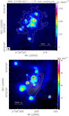 |
Fig. 1 Upper panel: NOEMA 1.37 mm continuum emission (color map) of IRAS 21078+5211. The white contours correspond to levels ranging from 3σ (σ = 0.5 mJy beam−1) to the peak intensity of 35 mJy beam−1, in steps of 7σ. The little black crosses indicate the positions of the seven strongest 1.37 mm peaks labeled as in Beuther et al. (2018, see Table 5), with label numbers ordered in intensity. The restoring beam of the 1.37 mm continuum map is shown in the lower left corner. Lower panel: Wide-field Infrared Survey Explorer (WISE) 4.6 μm image (color map, Wright et al. 2010) toward IRAS 21078+5211. The white contours represent the SCUBA 850 μm continuum (Di Francesco et al. 2008), showing 10 levels increasing logarithmically from 7σ (σ = 0.1 Jy beam−1) to 11.4 Jy beam−1. The magenta rectangle delimits the region plotted in the upper panel. |
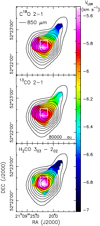 |
Fig. 2 IRAM 30 m data. Intensity-weighted velocity (color map) of the C18O J = 2–1 (upper panel), 13CO J = 2–1 (middle panel), and H2CO |

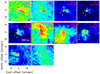 |
Fig. 3 Merged NOEMA–IRAM 30 m data. Each panel presents the emission of the 13CO J = 2–1 line (color map) in a different velocity channel. In the upper right corner of the panel, the channel VLSR (in kilometer per second) and the range of plotted intensity (in square parentheses in milliJansky per beam) are reported. The red boxes and ticks identify the panels corresponding to the central velocities, that is |VLSR − Vsys| < 3 km s−1. The white crosses mark the positions of the seven strongest peaks of the 1.37 mm continuum emission. At the central velocities, the black dashed line gives the major axis of the 1.37 mm core cluster. |
3.2 Cluster center: cores 1, 2, and 3
Toward cores 1, 2, and 3, the emission of the higher-excitation molecular lines is strong enough to allow us to study the kinematics and physical conditions of the gas. For this purpose, we used the XCLASS (eXtended CASA Line Analysis Software Suite) tool (Möller et al. 2017). This tool models the data by solving the radiative transfer equation for an isothermal homogeneous object in local thermodynamic equilibrium (LTE) in one dimension. It can produce maps of column density, temperature, velocity, and line width by extracting spectra pixel-by-pixel from the image cubes and fitting all the unblended lines of a given molecular species simultaneously. The finite source size, dust attenuation, and line opacity are considered as well, which also permitsus to properly fit the transitions of relatively lower-excitation energy and higher optical depths (as the CH3CN JK = 12K–11K, K = 0–2 lines).
To complement the XCLASS results, we also analyzed several, higher-excitation molecular lines, individually.We verified that the selected lines are sufficiently optically thin to reliably trace the more embedded gas kinematics. More specifically, in this analysis we made use of the following molecular lines: CH3CN JK = 12K–11K (K = 3–6), CH2CO  111,11–101,10, and HC3N J = 24–23. We fitted the line profile of these transitions toward the 1.37 mm continuum peak in core 1 and found that the optical depth is always < 0.5 at the peak velocity and decreases to values ≲0.05 across the line wings. The good quality of the fit for the CH3CN JK = 12K-11K (K = 0–6) lines is illustrated in Fig. 6.
We used XCLASS to simultaneously fit the emission of the CH3CN JK = 12K–11K (K = 0–6) lines (including the CH3 13CN isotopologs). Figure 7 shows the maps of the CH3CN column density and velocity toward the central plateau of the 1.37 mm continuum, where the three most intense cores reside. The CH3CN column density reaches 1016 cm−2 toward core 1 and it is a factor of 2 lower toward core 2. Two VLSR gradients are clearly detected: the first across the adjacent cores 1 and 3, characterized by a change of ≈ 4 km s−1 over ≈ 1500 au; the second across core 2, with a change of ≈ 3 km s−1 over ≈ 1000 au. In the following, we determine the velocities of the cores 1 and 3 to assess the contribution of their relative motion to the observed velocity gradient.
While the emission of the CH3CN JK = 12K–11K (K = 2–6) lines (with Eu∕kB varying in the range 97–326 K) is concentrated mainly toward core 1 (see Fig. 7, upper panel), we also identified a few molecular lines of slightly lower excitation, such as the CH2CO  111,11–101,10 transition (Eu∕kB = 76 K), which have comparable intensity toward cores 1 and 3 and can be employed to resolve the emission of the two cores in velocity. The upper panels of Fig. 8 show the maps of the peak emission of the CH3CN JK = 125–115 line toward core 1 and the CH2CO
  111,11-101,10 line toward core 3, while the lower panel of Fig. 8 reports the spectra of the two molecular lines integrated over the corresponding core. Among the CH3CN transitions, we selected the K = 5 component because it is intense and has a relatively high-excitation energy (Eu ∕kB = 247 K), which allows us to better resolve the warm gas inside core 1. To determine the areas of the two cores, we used the minimum level (18.6 mJy beam−1, indicated bythe black contours in Fig. 8) of the 1.37 mm continuum in correspondence of which two disconnected emission islands are still obtained. We stress that in this analysis we used the emissions of the CH3CN JK = 125–115 and CH2CO
  111,11–101,10 lines only to derive the velocities of the cores 1 and 3, whose existence and geometrical properties are independently established from the 1.37 mm continuum emission. The two cores are separated by ≈ 770 au and their LOS velocities differ by ≈ 3 km s−1. Therefore, it appears that the relative motion of the two cores can account for the observed VLSR gradient. This result is used in Sect. 4.1.2, where we consider the possibility that the two cores are members of a binary system.
Our recent H2 2.12 μm LBT observations toward IRAS 21078+5211 are shown in Fig. 9 (upper panel) together with the radio continuum and SO line emissions tracing the jet from YSO-1 and the molecular outflow from core 1, respectively. The H2 2.12 μm emission arises from shock-excited, compressed, and hot molecular gas placed ≈ 2′′ SW of core 1, pinpointed by the NE component of the radio jet at the center of the SO molecular outflow. Examining the lower panel of Fig. 9, which provides a higher-angular resolution view of the shock structure, we note two well-shaped bow shocks at the SW tips of the H2 2.12 μm emission. Since the major axes of these bow shocks approximately coincide with the directions to core 1, it is plausible that these shocks have been excited by an outflow emerging from core 1. Assuming that the outflow source resides in core 1, Fig. 9(upper panel) shows that different outflow tracers, namely, the nearby SW lobe of synchrotron emission, the weak 5 cm spur ≈ 7000 au to NE, and the H2 2.12 μm bow shock ≈40 000 au to SW, are oriented at different PAs. In Sect. 4.4, we discuss several scenarios to explain the spread in the directions of the various outflow tracers.
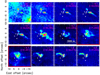 |
Fig. 4 Merged NOEMA–IRAM 30 m data. Each panel presents the emission of the SO JN = 65–54 line (color map) in a different velocity channel. In the upper right corner of the panel, the channel VLSR (in kilometer per second) and the range of plotted intensity (in square parentheses in milliJansky per beam) are reported. The red boxes and ticks identify the panels corresponding to the central velocities, that is |VLSR − Vsys| < 3 km s−1. The white crosses mark the positions of the seven strongest peaks of the 1.37 mm continuum emission. |
3.3 Most prominent core 1
Toward IRAS 21078+5211, the linear resolution achieved with the CORE data is ≈625 au (for a FWHM beam size of ≈0.′′38). As seen in Sect. 3.2, this is sufficient to resolve nearby molecular cores, on scales ≳1000 au. Star formation models predict that the gravitational pull of high-mass YSOs influences the gas kinematics mainly at distances ≤1000 au (see, for instance, Kölligan & Kuiper 2018), where kinematic structures such as accretion disks and disk winds (DW) are expected. Toward core 1, the high signal-to-noise ratio of the CH3CN JK = 12K–11K (K = 2–6) and other high-excitation molecular lines (such as OCS J = 18–17, HC3N J = 24–23, and HNCO  101,10–91,9) permits us to study the gas kinematics on linear scales ≤1000 au. For each of these strong molecular lines, we fit a 2D Gaussian profile to the emission in each velocity channel and determine the peak position as a function of velocity. If the emission is unresolved, the positional accuracy is equal to (δθ ∕ 2) × (σ ∕ I) (see, e.g., Reid et al. 1988), where δθ is the FWHM beam size and I and σ are the peak intensity and the rms noise, respectively, of a given channel. With an average value of the ratio (I ∕ σ) = 27, the error is ≲10 mas. For channels with resolved emission, the centroid positions convey more complex kinematic information because in these channels it is very likely that we are observing the combination of different types of motions and the shape of the emission can strongly deviate from a Gaussian. Consequently, for these channels the peak position obtained with the Gaussian fit is less reliable.
The upper panel of Fig. 10 shows the distribution of channel centroids for the CH3CN JK = 12K–11K (K = 3–6) and HC3N J = 24–23 lines, which are the most intense and compact molecular emissions in core 1. In Fig. A.1, the distribution of channel centroids is plotted separately for the CH3CN and HC3N lines to show that the two molecules have a very similar VLSR pattern. This allows us to combine their emissions in our kinematical analysis. The colored contours of Fig. 10, reproducing the half-peak emission levels, clearly indicate that the structure is really compact only at the most extreme red- and blue-shifted velocities. At VLSR ≈ −4 km s−1, the contamination from the nearby core 3 is evident. In the lower panel of Fig. 10 only the positions of the compact-emission channels at the extreme velocities are plotted. The distribution is bipolar and elongated along a direction, at PA = 123° ± 23°, approximately perpendicular to the radio jet. The compact 1.3 cm continuum emission, which best pinpoints the position of YSO-1, is located at the center of the distribution. In Sect. 4.2, we propose that the derived velocity pattern traces the accretion disk around YSO-1.
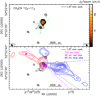 |
Fig. 5 Upper panel: NOEMA data. Velocity-integrated intensity (color map) of the CH3 CN JK = 123–113 line. The 1.37 mm continuum emission is represented with black contours, showing seven levels increasing logarithmically from 11 to 35 mJy beam−1. The positions of the three strongest peaks of the 1.37 mm continuum emission are indicated, using the same labels as in Beuther et al. (2018, see Table 5). The restoring beams of the CH3 CN JK = 123–113 line and 1.37 mm continuum maps are shown in the lower right and left corners, respectively. Lower panel: the blue and red contours reproduce the emission of the SO JN = 65–54 line integrated over the velocity ranges [−22,−13] and [−1, 5] km s−1, respectively. The plotted levels are from 0.03 to 2.5 Jy beam−1, in steps of 0.27 Jy beam−1, and from 0.6 to 2.2 Jy beam−1, in steps of 0.37 Jy beam−1, for the blue- and red-shifted SO emission, respectively. The magenta contours give the JVLA A-Array continuum at 5 cm (Moscadelli et al. 2016), showing levels at 40, 50, and 90% of the peak emission of 95 μJy beam−1: the magenta dashed line connects the two strongest (nearby, but resolved) 5 cm peaks. The two black dashed lines delimit the viewing angle of the blue-shifted emission of the SO JN = 65–54 line from the NE 5 cm peak (aligned in position with core 1, see Sect. 3.1). The black contours have the same meaning as in the upper panel. |
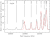 |
Fig. 6 Beam-averaged spectrum (black line) of the CH3CN JK = 12K–11K (K = 0–8) line emissiontoward the 1.37 mm continuum peak. The positions of the K = 0–8 lines are indicated. The fits (red histograms) of the K = 0–6 lines performed with XCLASS are also shown. |
4 Discussion
4.1 The cluster
4.1.1 Mass flow toward the core cluster
The 1.37 mm continuum cluster is found at the density peak of a SE-NW elongated molecular cloud edged on the northeastern side with a necklace of less embedded YSOs and on the southwestern side with a filament of diffuse 4.6 μm emission (see Fig. 1, lower panel). These findings suggest that the molecular cloud is a density enhancement of a more extended, infrared dark filament. In Sect. 3.1 we showed that the velocities of the slow-moving (≤ 3 km s−1) gas of the cloud and the cluster vary smoothly along the major axis of the molecular cloud over linear scales of 104 –105 au (see Figs. 2 and 3). This regular change in VLSR with position makes us favor the interpretation in terms of a flow in the molecular gas (converging toward the density peak where the most massive cores reside) compared with cloud-cloud collision, which would rather appear as a sudden jump in velocity. In the assumption of a mass flow, the observed VLSR gradient can be easily explained if the blue-shifted NW side of the molecular cloud is farther away from us than the red-shifted SE side. The spatial and velocity extents of this VLSR gradient are comparable with those of the gradients, ~1 km s−1 per 0.1 pc, observed in infrared dark clouds (IRDC) at the sites of YSOs (Ragan et al. 2012), which are often interpreted as infall. It is also consistent with simulations of large-scale accretion flows along filaments, gravitationally accelerated toward local density peaks (see, e.g., Tobin et al. 2012; Smith et al. 2013).
Assuming we are observing a mass infall toward the core cluster, we can use both the IRAM 30 m and merged NOEMA–IRAM 30 m observations of the 13CO J = 2–1 line to calculate the mass infall rate. The latter can be derived from the ratio of the momentum, Pinf, to the length, Linf, of the flow. In Appendix B, we describe the method to calculate the momentum of a molecular outflow, by employing the 13CO J = 2–1 emission. The same equations hold to derive the momentum of a molecular infall as well. We employ the same parameters used for the 13CO J = 2–1 molecular outflow (see Table B.1) with the following exceptions. First, the velocities to be considered are those within a small interval about the systemic velocity, that is, [−7, −5.5] km s−1 for the IRAM 30 m observations (see Fig. 2), and [−6.5, −3.5] km s−1 for the merged NOEMA–IRAM 30 m data (see Fig. 3). Second, the FWHM size of the map beam is Bmax = Bmin = 11.′′8, for the IRAM 30 m observations. It is remarkable that, using either the IRAM 30 m or the merged NOEMA–IRAM 30 m observations, we obtain very consistent values for the infall momentum Pinf cos(iinf) ≈ 28 M⊙ km s−1, where iinf is the inclination angle of the flow with respect to the LOS. Taking Linf sin(iinf) ≈ 6 × 10⁴ au, corresponding to the average value between the (sky-projected) flow lengths measured in the IRAM 30 m (8 × 10⁴ au, see Fig. 2) and NOEMA-IRAM 30 m (4 × 10⁴ au, see Fig. 3) maps, we finally derive a mass infall rate Ṁinf cot(iinf) = Pinf cos(iinf) ∕ Linf sin(iinf) ≈ 28 M⊙ km s−1 / 6 × 10⁴ au ≈ 10−4 M⊙ yr−1. Following the discussion in Appendix B, owing to the uncertainties in the excitation temperature of the 13CO J = 2–1 line and abundance ratio of 13CO, our estimateof the infall rate should be accurate to within a factor of 5. The derived value of infall rate falls at the lower end of the range oflongitudinal flow rates measured in filaments associated with high-mass star-forming regions (Chen et al. 2019; Treviño-Morales et al. 2019).
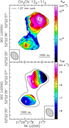 |
Fig. 7 NOEMA data. The color map reproduces the column density (upper panel) and the velocity (lower panel) of the CH3 CN emission determined by fitting with XCLASS the CH3CN JK = 12K–11K (K = 0–6) lines (including the CH3 13CN isotopologs), simultaneously. The plotted regions correspond to the areas in which the 1.37 mm continuum emission is higher than 13 and 16 mJy beam−1 for the column density and velocity plots, respectively. The 1.37 mm continuum emission is represented with black contours, showing six levels increasing logarithmically from 13 to 35 mJy beam−1: the positions of the three strongest 1.37 mm peaks are denoted using the same labels as in Beuther et al. (2018, see Table 5). The restoring beams of the 1.37 mm continuum and CH3 CN maps are shown in the lower left corner of the upper panel and lower right corner of the lower panel, respectively. |
4.1.2 Temperature and mass distribution over the cluster center
Figure 11 shows the rotational temperature determined with XCLASS by simultaneously fitting the emission of the CH3CN JK = 12K–11K (K = 0–6) lines (including the CH3 13CN isotopologs). While toward core 1 the gas temperature is always ≥115 K and may reach 200 K, toward core 3 it varies in the range 90–130 K. In correspondence of core 2 the temperature map is less homogeneous, probably owing to insufficient signal-to-noise ratio, and has an average temperature that is intermediate between that of core 1 and core 3. By combining the maps of the 1.37 mm dust continuum and gas temperature, assuming that the dust emission is optically thin, we can make a reasonable estimate of the core masses. For consistency with Beuther et al. (2018), we adopt a dust absorption coefficient of 0.9 cm2 g−1 (Ossenkopf & Henning 1994) and a gas-to-dust mass ratio of 150 (Draine 2011). Over the areas of core 2 and the combined cores 1 and 3 (see Fig. 11), the mass is found to be 0.46 and 0.92 M⊙, respectively.Inside the individual cores 1 and 3, whose corresponding areas are delimited by the black contours in the upper panels of Fig. 8, we obtain a gas mass of 0.42 M⊙ and 0.12 M⊙, respectively. These values represent the mass inside the cores within radii ≤500 au, and they are lower than the total core masses determined by Beuther et al. (2018, see Table 5) over radii ≥1000 au with a mean gas temperature of 66 K.
In Sect. 3.2, using the CH3CN JK = 12K–11K (K = 0–6) lines (see Fig. 7), we traced the kinematics of the gas inside the three cores in the cluster center. Now, we use this result to derive the dynamical masses of the cores and estimate the masses of the embedded YSOs. In Sect. 4.2.2 we determine the mass of YSO-1 (the YSO inside core 1) to be 5.6 ± 2.0 M⊙. In Sect. 3.2, we showed that the VLSR gradient across the adjacent cores 1 and 3 can be well explained in terms of the relative motion of the cores. Assuming that we are observing rotation seen almost edge-on, in gravito-centrifugal equilibrium, from the spatial separation between the cores, ≈770 au, and their difference in velocity, ≈3 km s−1 (see Sect. 3.2), we derive a total mass of ≈8 M⊙. Subtractingboth the mass of YSO-1 of ≈5.6 M⊙ and that (0.92 M⊙, see above) of the gas embedded inside cores 1 and 3, we obtain a rough estimate for the mass of the YSO inside core 3 of ≈1–2 M⊙. Regarding core 2, interpreting the VLSR gradient (≈3 km s−1 across ≈1000 au, see Sect. 3.2) observed toward this core as rotation, in gravito-centrifugal equilibrium, we derive a dynamical mass of ≈2.5 M⊙. After subtracting the gas mass of 0.46 M⊙ (see above), the derived mass for the YSO inside core 2 is ≈2 M⊙. Despite the large uncertainty in these determinations, the presence of relatively low-mass YSOs inside cores 2 and 3 agrees with the lower temperature (see Fig. 11) and mass of these cores with respect to core 1.
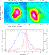 |
Fig. 8 NOEMA data. Upper panels: the color maps reproduce the emission of the CH3 CN JK = 125–115 (left) and CH2CO |


4.1.3 Present state and future evolution
Among the 20 cores identified in the 1.37 mm continuum emission of IRAS 21078+5211 by Beuther et al. (2018, see Table 5), only cores 1, 2, and 3, which are the most massive (≥2 M⊙), show signatures of an embedded protostar. As described in Sect. 3.1 (see also Fig. 5, upper panel), the higher-excitation molecular lines are only detected toward these three cores, indicating that they are sufficiently warm to require local heating by a protostar. Fitting the CH3CN JK = 12K–11K lines, the gas temperature over the three cores is found everywhere ≳100 K (see Sect. 4.1.2), and, through the observed VLSR gradients (see Sect. 3.2), the masses of the embedded YSOs are evaluated in the range 1–6 M⊙ (see Sect. 4.1.2). The concentration of the most massive cores (and YSOs) toward the center of the 1.37 mm continuum cluster hints at mass segregation.
Judging the evolutionary state of the other, less massive cores is difficult with the present observations. Comparing with the most massive cores, the non-detection toward these cores of the higher-excitation molecular lines indicates an upper limit of ≲ 1 M⊙ for the mass of the embedded YSOs. The fact that no molecular outflows are detected from the less massive cores (see Sect. 3.1) would be consistent with most of these cores still being in a prestellar phase. However, with our data, a molecular outflow is observed only from the most massive YSO, YSO-1 in core 1, and this hints at a sensitivity limit when using the 13CO J = 2–1 and SO JN = 65–54 lines as outflow tracers. Future interferometric observations in the CO J = 2–1 line, more intense and with broader excitation conditions, could unveil less massive and energetic outflows. On a more speculative ground, the non-detection of outflows from the less massive cores could be also explained if the (putative) embedded low-mass YSOs were not actively accreting because most of the gas available across the cluster was gathered by YSO-1.
To discuss the future evolution of the IRAS 21078+5211 core cluster is useful to compare it with more evolved states as the well-studied, NIR stellar clusters around Ae or Be pre-main-sequence (PMS) intermediate-mass (1–6 M⊙) stars (see, for instance, Testi et al. 1999). Ae and Be PMS stars are young enough, 0.5–5 Myr, that any population of lower-mass stars born in the same environment did not have enough time to move away from the birthplace. Therefore, the spatial distribution of the stars reflects that of the parental molecular cores. The typical size of these NIR stellar clusters is ≈0.2 pc, and the highest stellar densities, up to 103 pc−3, are found in correspondence with the most massive (≈6 M⊙) Ae or Be stars. In IRAS 21078+5211, 20 cores are detected over an area of ≈ 10−2 pc2, equivalent to a density of 2 × 10⁴ pc−3, and the most massive YSO (YSO-1) has already attained a mass close to 6 M⊙. In Sect. 4.1.1, we calculated a mass infall rate of ~10−4 M⊙ yr−1 from the parental molecular cloud (total mass of 177 M⊙, Beuther et al. 2018, see Table 1) to the core cluster, which, over the characteristic formation time of a few 105 yr of the Ae and Be PMS stars (Palla & Stahler 1993), would imply an infall toward the cluster of a few 10 M⊙. If a relevant fraction of this mass is accreted by the most massive YSOs at the center of the cluster, it is very likely that at least one high-mass (≥8 M⊙) star will form. In conclusion, because of the relatively high stellar density and the likelihood of ultimately forming massive stars, we think that the IRAS 21078+5211 core cluster can be the progenitor of a stellar system whose most massive members are early B or late O-type high-mass stars, rather than Ae or Be intermediate-mass stars.
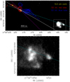 |
Fig. 9 Comparison of CORE, POETS and LBT observations. Upper panel: the gray-scale map reproduces the H2 2.12 μm emission observed with LBT toward IRAS 21078+5211. Referring to Fig. 5, lower panel, the blue and red contours have the same meaning, and the yellow contours replace the magenta contours for the JVLA 5 cm continuum. The magenta dashed, white dotted, and cyan dashed lines connect the main 5 cm peak with the secondary (nearby) 5 cm peak, the weak 5 cm spur to NE, and the bow shock traced by the LBT H2 2.12 μm emissionto SW, respectively. The white dashed box delimits the region plotted in the lower panel. Lower panel: adaptive-optics assisted LBT observations of the H2 2.12 μm emission (gray-scale map): the cyan dashed line has the same meaning as in the upper panel. |
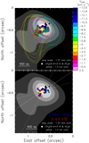 |
Fig. 10 NOEMA data. Upper panel: the gray-scale map reproduces the 1.37 mm continuum emission, plotting values in the range 10–35 mJy beam−1. The colored dots give the (Gaussian-fitted) positions of the channel emission peaks for the CH3 CN JK = 12K–11K (K = 3–6) and HC3N J = 24–23 lines; the colors denote the channel VLSR. The colored contours indicate the half-peak level for the CH3CN JK = 123-113 emission in individual channels. The yellow contours show the JVLA A-Array continuum at 1.3 cm (Moscadelli et al. 2016), showing levels at 70, 80, and 90% of the peak emission of 0.50 mJy beam−1. Lower panel: the gray-scale map, yellow contours, and colored dots have the same meaning as in the upper panel. Only the channel emission peaks at the extreme blue- and red-shifted velocities (reported in the lower right corner of the panel) are shown. The white continuous and dashed lines indicate the best-fit major axis of the distribution of the peaks and the corresponding fit uncertainty, respectively. |
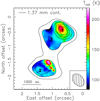 |
Fig. 11 NOEMA data. The color map shows the distribution of the rotational temperature derived by fitting with XCLASS the emission of the CH3CN JK = 12K–11K (K = 0–6) lines (including the CH3 13CN isotopologs). The plotted region corresponds to the area in which the 1.37 mm continuum emission is higher than 16 mJy beam−1. The black contours reproduce the 1.37 mm continuum, showing the same levels as in Fig. 7: the positions of the three strongest 1.37 mm peaks are indicated using the same labels as in Beuther et al. (2018, see Table 5). The restoring beam of the CH3 CN maps is shown in the lower right corner of the panel. |
4.2 Disk-jet system associated with YSO-1
4.2.1 Radio jet and molecular outflow
Absolute positions and proper motions of the 22 GHz water masers observed in IRAS 21078+5211 with the POETS survey are presented in Fig. 12. The water masers show a SW-NE elongated distribution at radii between 100 au and 300 au from the peak of the compact 1.3 cm JVLA continuum, corresponding to the core of the radio jet and the YSO-1 position. The elongation, at PA ≈ 38°, of the maser spatial distribution, and the average direction of the proper motions, PA ≈ 49° (Moscadelli et al. 2019,see Table A1), are in good agreement with the orientation, PA ≈ 43°, of the double-component radio jet (see Fig. 5). The faint, thermal, and nonthermal emissions from the NE and SW radio lobes, respectively, and the water masers are all manifestations of different types of shocks produced by the jet. In the jet core, close to YSO-1, we observe free-free emission, which likely originates from relatively weak (C-type), internal shocks of the jet corresponding to changes in the mass loss or ejection velocity (Moscadelli et al. 2016; Anglada et al. 2018); the nonthermal emission is likely synchrotron emission from electrons accelerated at relativistic velocities in strong jet shocks through first-order Fermi acceleration (Bell 1978); finally, the fast water masers emerge from relatively strong (J-type) shocks, whereas the jet impinges on very dense (molecular hydrogen number density,  cm−3) ambient material at high velocity (Moscadelli et al. 2020).
As reflected in Fig. 5 (lower panel), the radio jet and the molecular outflow traced by the SO JN = 65–54 line at larger scales are approximately parallel to each other and, as already anticipated in Sect. 3.1, the molecular outflow could be powered by the jet. To assess the physical association between the jet and molecular outflow, in the following we determine and compare their physical properties. In Appendix B, we describe the method to calculate the momentum of the molecular outflow, Pout. We obtain Pout cos(iout) ~ 50 M⊙ km s−1, where iout is the inclination angle of the outflow with respect to the LOS. Employing the water maser positions and three-dimensional (3D) velocities, the momentum rate of the jet in IRAS 21078+5211 was estimated to be Ṗjet ~ 1 × 10⁻³ M⊙ km s−1 yr−1 by Moscadelli et al. (2016, see Sect. 6.2, Eq. (1), and Table 5). In this calculation, a major source of uncertainty was the pre-shock, ambient density, which was assumed to be  108 cm−3. Now, thanks to the CORE data, we can better constrain this parameter. Averaging the derived mass distribution (see Sect. 4.1.2) over a cylindric volume equal to the beam area times the beam size, in the direction of the continuum peak we find the value
  3 × 108 cm−3, which should be accurate to within a factor of a few. Accordingly, our new, more precise, estimate of the momentum rate of the jet is Ṗjet ~ 3 × 10⁻³ M⊙ km s−1 yr−1.
We wish to derive the momentum rate of the molecular outflow, to be compared with that of the jet. Knowing the value of Pout cos(iout) (see above), we need to estimate the inclination angle and timescale of the outflow. The clear spatial separation of the blue- and red-shifted lobes (see Fig. 5, lower panel) indicates that the gas flows along directions significantly inclined with respect to both the LOS and the plane of the sky. Based on the opening angle of ≈ 40° of the blue-shifted outflow lobe (see Fig. 5, lower panel), we judge that the outflow axis has to be at least 20° away from both the LOS and the plane of the sky, that is 20 ≤ iout ≤ 70°. The dynamical timescale of the outflow, tout, can be estimated from the ratio of the size of the lobes to the corresponding maximum VLSR range. Referring to the SO JN = 65–54 emission in Fig. 5 (lower panel), we have: tout tan(iout) ≈ 22′′ / 27 km s−1 = 6.3 × 10³ yr, at a distance of 1.63 kpc. We caution that previous studies have pointed out that the dynamical timescale of molecular outflows can largely underestimate (by a factor between 5 and 10) the true outflow age (see, for instance, Parker et al. 1991). Accordingly, the upper limit for the momentum rate of the outflow is found to be Ṗout cos 2(iout) / sin (iout) ≲ 8 × 10⁻³ M⊙ km s−1 yr−1. Consideringthat this value is only accurate to within an order of magnitude and that 0.4 ≤ sin(iout) / cos 2(iout) ≤ 8 for 20° ≤ iout ≤ 70°, we conclude that the momentum rate of the molecular outflow is consistent with that of the jet. It is then plausible that the jet powers the molecular outflow.
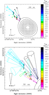 |
Fig. 12 POETS water maser observations. Upper panel: colored dots and arrows give absolute positions and proper motions of the 22 GHz water masers determined with VLBI observations (Moscadelli et al. 2016); colors denote the maser VLSR. The dot area scales logarithmically with the maser intensity. The black contours indicate the JVLA A-Array continuum at 1.3 cm (Moscadelli et al. 2016), showing levels from 10 to 90% of the peak emission of 0.50 mJy beam−1 in steps of 10%. Lower panel: colored dots and black contours have the same meaning as in the upper panel. Colored cones are employed to visualize the maser 3D velocities, representing the inclination with respect to the LOS through the ellipticity of the cone basis and the uncertainty in the direction by means of the cone aperture. |
4.2.2 Mass and luminosity of YSO-1
The velocitypattern in Fig. 10 (lower panel) is consistent with that expected for a rotating disk around a YSO. It is elongated approximately perpendicular to the radio jet, the blue- and red-shifted velocities lie on the two sides of the YSO, and its size of ≈ 400 au agrees with the model predictions for accretion disks around high-mass YSOs (see, for instance, Kölligan & Kuiper 2018). The VLSR does not present a regular change with the position, but that likely results from the limited precision in tracing the velocity pattern using channel emission centroids and the insufficient angular resolution.
Making the assumption (to be checked a posteriori, see below) of Keplerian rotation, we determine the central mass, M⋆, by minimizing the following χ2 expression:
![\begin{equation*}\chi^2\,{=}\,\sum_j \frac{ [ V_j - (V_{\star} \,{\pm}\, 0.74 \; (M_{\star} \sin^2(i_{\textrm{rot}}))^{0.5} \; \; | S_j-S_{\star} |^{-0.5} \,) ]^2 } {(\Delta V_{j})^2} ,\end{equation*}](/articles/aa/full_html/2021/03/aa39837-20/aa39837-20-eq10.png) (1)
(1)
where Vj and Sj are the channel VLSR (in kilometer per second) and corresponding peak positions (in arcsecond), the index j runs over all the fitted channels, and the + and − symbols hold for red- and blue-shifted velocities, respectively. V⋆ (in kilometer per second) and S⋆ (in arcsecond) are the VLSR and position of YSO-1, respectively. The central mass M⋆ is given in solar masses. Indicating with irot the inclination of the disk rotation axis with respect to the LOS, the factor sin 2(irot) takes into account that the disk plane is seen at an angle 90 − irot from the LOS and the observed VLSR corresponds to the rotation velocity multiplied by the factor sin(irot). To take into account the uncertainty on the velocity and that on the position, the global velocity error ΔVj is obtained by summing in quadrature two errors: that on the velocity (taken equal to half of the channel width) and that obtained by converting the error on the offset into a velocity error through the function fitted to the data.
The VLSR, V⋆ = − 6.4 km s−1, and position S⋆ = 0.′′81 of YSO-1 are assumed equal to the average of the VLSR and positions of all the channels. Thus, the term M⋆ sin2(irot) is the only free parameter in Eq. (1). We allowed this term to vary over the range 2–14 M⊙, which is consistent with the upper limit of ≈ 12 M⊙ imposed by the bolometric luminosity of ≈104 L⊙ (Davies et al. 2011). Figure 13 reports the plot of the χ2 vs. the free parameter; the blue dashed lines delimit the 1σ confidence interval following Lampton et al. (1976). This plot shows that we do find an absolute minimum of the χ2 and the determined 1σ range for the values of the free parameter is M⋆ sin2(irot) = 5.3 ± 1.6 M⊙.
The fitted value of M⋆ is much larger than the gas mass, 0.42 M⊙, inside core 1, derived from the dust emission in Sect. 4.1.2. As noted in Sect. 4.1.2, this is the mass inside core 1 within a radius ≤500 au, which is comparable to the size of the disk structure traced by the CH3CN and HC3N lines around YSO-1 (see Fig. 10, lower panel). The YSO-1 envelope should extend at significantlylarger radii and be much more massive. The finding that the central mass is much greater than the mass of the disk supports our assumption of Keplerian rotation. The disk, traced by the bipolar VLSR pattern of molecularemissions (see Fig. 10, lower panel), and the radio-maser jet are approximately perpendicular to each other in the plane of the sky. This suggests that the jet is directed close to the rotation axis of the disk, or ijet ≈ irot (where ijet is the inclination of the jet with respect to the LOS). From the angular distribution of the maser proper motions, reported in Fig. 12, the semi-opening angle of the jet is evaluated to be ≈ 18° by Moscadelli et al. (2016, see Table 5). Figure 12, lower panel, also shows that the water masers are both blue- and red-shifted, which indicates that the jet intersects the plane of the sky and the relation |ijet− 90°|≲ 18° must hold. Following these considerations, we can write sin2(irot) ≈ sin2(ijet) ≳ sin2(72°) = 0.9. Allowing for the variation of the factor sin2(irot) in the range 0.9–1, the 1σ interval for the fitted YSO-1 mass is M⋆ = 5.6 ± 2.0 M⊙.
By employing the relationship between bolometric luminosity, Lbol, and outflow momentum rate, Ṗ, for massive YSOs by Maud et al. (2015) (Log10 [Ṗ ∕ M⊙ km s−1 yr−1] = −4.8 + 0.61 Log10 [Lbol ∕ L⊙]), and our best estimate of the momentum rate Ṗjet ~ 3 × 10⁻³ M⊙ km s−1 yr−1 (see Sect. 4.2.1), we infer a luminosity of 5 × 10³ L⊙ for YSO-1. This value is consistent with the luminosity of 1.3 × 10⁴ L⊙ of the IRAS 21078+5211 region, which was derived by Molinari et al. (1996) using low-angular resolution IRAS data (~1′, Neugebauer et al. 1984) only8. Indeed, combining the far-infrared IRAS fluxes with the mid-infrared, Wide-Field Infrared Survey Explorer (WISE; Wright et al. 2010) and Midcourse Space Experiment (MSX; Egan et al. 2003) data at higher angular resolution (~10′′), Moscadelli et al. (2016, see Table 1) determine a lower luminosity of 5 × 10³ L⊙, which agrees well with that inferred for YSO-1.
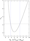 |
Fig. 13 χ2 values from the Keplerian fit (see Eq. (1)) vs. the free parameter M⋆ sin 2(irot). The horizontal black dashed line indicates the value |

4.3 Magnetized and rotating jet
The radio-maser jet emerging from YSO-1 is unique in combining two properties that, to our knowledge, for the first time are observed associated with the same object: a lobe with nonthermal emission and jet rotation. We noted the first point several times through this article and this refers to the SW lobe of the double-component radio jet (see Fig. 5, lower panel), whose spectral index over the frequency range 6–22 GHz is ≤ −0.7 (Moscadelli et al. 2016, see Table 4 and Fig. 19). Observations of nonthermal components in jets from high-mass YSOs are still rare, although good examples were recently discovered thanks to high-angular resolution, sensitive radio survey (for instance, the POETS source G035.02+0.35, Sanna et al. 2019). The observational evidence for the second point, as already discussed in Moscadelli et al. (2019, see Sect. 3.2), is the VLSR gradient of the water masers transversal to the jet direction. Figure 12 (lower panel) shows the monotonic change of the maser VLSR along a SE-NW direction perpendicular to the SW-NE collimation axis of the proper motions, with red- and blue-shifted VLSR toward SE and NW, respectively. The linear correlation between the maser LOS velocities, VLOS = VLSR − V⋆, and positions projected perpendicular to the jet direction, Rper, is clearly illustrated in Fig. 14. A straightforward interpretation for the maser 3D velocity pattern is in terms of a composition of two motions: a flow along, and a rotation around, the jet axis.
The findings of nonthermal emission from a jet lobe and jet rotation are strong indications that magnetic fields play an important role in both launching and accelerating the jet. The interpretation of the nonthermal continuum in terms of synchrotron emission requires the presence of a magnetic field sufficiently ordered and strong to trap electrons in jet shocks, confine them even at relativistic velocities, and warrant the detection of their synchrotron signal. Jet rotation is considered a critical test for magneto-centrifugal (MC) DW (Blandford & Payne 1982; Pudritz et al. 2007), where the magneto-centrifugally launched jetextracts the excess angular momentum from the disk gas, which, then, can be accreted by the protostar. Comparing Figs. 10 and 12, we evince that the jet and the disk of YSO-1 rotate about axes approximately parallel to each other and have the same sense of rotation, that is, toward and away from us to NW and SE, respectively.This result supports our idea that the jet rotation stems from the disk through the magnetic leverage of a MC DW.
The measurement of the 3D velocities of the jet near the YSO through water maser VLBI observations permits a more quantitative comparison with the predictions of the MC DW theory. According to the MC DW models (Pudritz et al. 2007), the YSO wind is centrifugally launched along the magnetic field lines threading the accretion disk, it is accelerated to the Alfvén speed sliding along the rotating field lines, and then is magnetically collimated. A large body of different MC DW simulations have shown that, depending on the assumed magnetic field configuration, the final jet structure can be either collimated toward a cylinder or at wide angle (Pudritz et al. 2007). In the following, we compare our water maserobservations with wind models that recollimate within a cylindrical flow tube (see, for instance, the simulations in Staff et al. 2015 and Kölligan & Kuiper 2018). We also note that a model of a cylindrical rotating jet has been recently proposed by Burns et al. (2015) to interpret the 3D motion of the water masers observed with VERA (VLBI exploration of radio astrometry; Kobayashi et al. 2003) toward the massive YSO S235AB-MIR.
Let us indicate with r0 the radius of the footpoint of the magnetic field line anchored to the disk and with rA the distancefrom the rotation axis at which the wind velocity equals the Alfvén speed. At radii rc ≥ rA, the wind recollimates, and its velocity has two (dominant) components: the main component oriented along the jet axis, ϒaxi, and the azimuthal component, ϒΦ, representing the rotation around the axis. Combining Eqs. (12) and (13) of Pudritz et al. (2007), the ratio of these two components can be related to the radius rc of the cylindrical flow through the expression
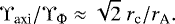 (2)
(2)
The water masers originate in shocks that arise where the jet impinges on high-density material and propagate away along the jet direction at a speed, assuming momentum conservation, V =  ϒ (see, for instance, Masson & Chernin 1993). In this equation, ρjet and ϒ are the jet density and speed, respectively, and ρamb is the ambient density. Since the water masers move parallel to the wind, their motion can be described in terms of the composition of the same velocity components, that is, that directed along the jet axis and the azimuthal component. Let us indicate with Vaxi and Vper the maser velocity components in the plane of the sky parallel and perpendicular to the sky-projected jet axis (at PA = 43°). Since the jet is directed close (≤18°, see Sect. 4.2.2) to the plane of the sky, Vaxi approximates the component along the jet axis with a maximum error of cos −1(18°) ≈ 5%. The azimuthal component, VΦ, is equally well approximated with
  . From the considerations above, it is clear that the ratio of the maser velocity components Vaxi and VΦ is an accurate measurement of the corresponding ratio of the wind velocity components, that is, ϒaxi ∕ ϒΦ ≈ Vaxi ∕ VΦ.
Figure 15 shows that the ratio Vaxi ∕ VΦ is approximately constant for the vast majority of the water masers (with measured proper motions). We obtain Vaxi ∕ VΦ ≈ 3.4 ± 1. The only notable exception is a small maser cluster at the most blue-shifted velocities (VLOS ≤ −20 km s−1) closer to YSO-1 (axis-projected separation Raxi ≤ 150 au), for which 1 ≲ Vaxi ∕ VΦ ≲ 2. On the basis of Eq. (2), a simple explanation for the small spread in the ratio of the maser velocity components is that most of the masers originate within a thin cylindrical shell, tracing shocked wind material MC-launched within a thin annulus of radius r0 of the rotatingdisk. This interpretation fits with the models predicting a shock origin for the water masers, since it is plausible that the most external layer of the jet mainly interacts with the surrounding ambient material and the water masers are mainly found on the jet wall. Thus, a reasonable estimate for the radius of the jet, rjet, can be obtained from half the spread in Rper, the maser positions projected perpendicular to the jet direction, considering only the water masers with VLOS ≥ −20 km s−1 (see Fig. 14). We derive rjet ≈ 10 mas, or ≈16 au.
The terminal poloidal velocity of a MC DW, which for a cylindrical flow corresponds to ϒaxi, can be approximated as (Pudritz et al. 2007, see Eq. (12))
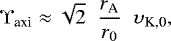 (3)
(3)
where υK,0 is the disk Keplerian velocity at the radius r0. From Eq. (2) and knowing both the ratio of ϒaxi / ϒΦ ≈ 3.4 and the radius rc = rjet ≈ 16 au, we get rA ≈ 6.7 au. Numerical and theoretical models (for a review see Pudritz et al. 2007) supported by observations (Bacciotti et al. 2002) constrain the ratio of rA ∕r0 ≈ 3. Then, using the above value of rA we infer r0 ≈ 2.2 au. From the latter and the estimated mass of YSO-1 M⋆ ≈ 5.6 M⊙, we find υK,0 ≈ 50 km s−1, which, through Eq. (3), yields ϒaxi ≈ 200 km s−1 and ϒΦ ≈ 200 km s−1 / 3.4 ≈ 60 km s−1.
The derived values of jet radius and terminal velocity are in reasonable agreement with the few measurements of spatially resolved radio jets from intermediate-mass YSOs (Anglada et al. 2018, see Table 1) and the results from high-resolution, 3D numerical simulations of MC DWs to 100 au scale (Staff et al. 2014, see Fig. 3). It is also plausible that our estimate for the jet rotational velocity is larger than the values of a few 10 km s−1 typical for jets from low-mass YSOs (Bacciotti et al. 2002; Coffey et al. 2004; Ray et al. 2007). The ratio of the maser to the jet speeds depends on the density contrast between the jet and the ambient medium through V / ϒ =  . High-angular resolution observations toward low-mass (Podio et al. 2015; Gómez-Ruiz et al. 2015) and high-mass (Anglada et al. 2018) YSOs, which are also supported by recent numerical simulations of MC-DWs (Staff et al. 2019, see Fig. 5), indicate values of
  cm−3 for the density of the high-velocity gas in jets. From this value and our measurement of the average ambient density in core 1
  cm−3, we derive V / ϒ ~ 0.1. This agreeswith the ratio of the maser-averaged value of Vaxi = 23 km s−1 to the estimate for ϒaxi ≈ 200 km s−1.
A key prediction of the MC DW theory is that the wind mass flux is about 10% of the accretion flux (Pudritz & Ray 2019). Assuming that YSO-1 gathers most of the mass flowing toward the core cluster from the parental molecular cloud, its accretion rate can be estimated as Ṁacc ≈Ṁinf ≈ tan (iinf) 10−4 M⊙ yr−1 (see Sect. 4.1.1). Combining the jet momentum rate Ṗjet ~ 3 × 10⁻³ M⊙ km s−1 yr−1 (see Sect. 4.2.1) with the jet terminal velocity ϒaxi ≈ 200 km s−1 derived above, the mass ejection rate of YSO-1 is found to be Ṁeje ≈ 1.5 × 10⁻⁵ M⊙ yr−1. Thus, the ratio of the ejection and the accretion rates is Ṁeje ∕ Ṁacc ≈ 0.15 cot(iinf). For an intermediate value of (the inclination of the infall) iinf ≈ 55°, this ratio is consistent with the value of ≈0.1 predicted by the MC DW theory.
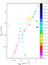 |
Fig. 14 Maser positions projected perpendicular to the jet axis, Rper, vs. corresponding LOS velocities, VLOS, for the masers with VLOS ≥ −20 km s−1. Colored error bars are used to indicate values and associated errors; the colors represent the distance from YSO-1 projected along the jet axis, Raxi, as coded in the wedge on the right-hand side of the panel. The black dashed line shows the linear fit to the plotted values. |
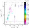 |
Fig. 15 Components Vaxi vs. VΦ (see definitions in Sect. 4.3) for the 3D maser velocities shown in Fig. 12. Colored error bars are used to indicate values and associated errors; the colors represent the distance from YSO-1 projected along the jet axis, Raxi, as coded in the wedge on the right-hand side of the panel. The black dashed line shows the linear fit to the subset of points within the region delimited by the horizontal and vertical black dotted lines, corresponding to VΦ ≤ 20 km s−1 and Vaxi ≥ 5 km s−1. |
4.4 Change in the jet direction
Since there is no hint of multiple YSOs inside core 1 in our data, the different direction of the outflows from core 1 shown in Fig. 9 (upper panel) is most likely due to a change in the orientation of the jet ejected from YSO-1. The angle between the direction, at PA = 71°, to the far H2 bow shock and the axis of the compact radio jet, is ≈28°. From previous studies of jet precession (see, for instance, Fendt & Zinnecker 1998; Shepherd et al. 2000) and recent 3D magnetohydrodynamics (MHD) simulations of protostar formation (see, for instance, Hirano & Machida 2019), it is known that several processes can produce a large (≥ a few 10°) change in the jet orientation: (1) radiation-induced warping of the protostellar accretion disk; (2) tidal interactions between the disk around the primary and the secondary, within a close binary system; (3) anisotropic accretion; and (4) magnetic braking. In the following, we discuss each of these points. We can readily exclude the first point, since the mass and luminosity of YSO-1 is not sufficient to warp the disk. By employing Eq. (1) of Shepherd et al. (2000), we find that the size of the observed disk is orders of magnitude smaller than the critical value beyond which the disk can be unstable to warping.
Concerning now the second point, we consider the binary system of YSOs inside the adjacent cores 1 and 3 (see Sect. 4.1.2). Assuming that the disk surface density is uniform, for Keplerian rotation, the precession frequency is given by the expression (Terquem et al. 1999, see Eq. (1))
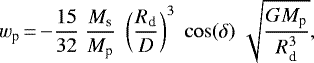 (4)
(4)
where Mp and Ms are the masses of the primary and secondary stars, respectively, Rd and D are the disk radius and binary separation, respectively, and δ is the inclination angle of the binary orbit with respect to the plane of the disk. From Sects. 4.1.2 and 4.2.2, we have Mp = M⋆ ≈ 5.6 M⊙, Ms ∕Mp ≈ 0.25, D ≈ 770 au. Referring to Fig. 10 (lower panel), Rd ≈ 250 au is estimated by taking half the spread in position (projected along the major axis of the distribution at PA = 123°) for the high-velocity molecular emissions tracing the YSO-1 disk. The line, at PA = 129°, connecting the dust emission peaks of cores 1 and 3 and the disk major axis form a small angle of ≈ 6°, which corresponds to the projection of δ on the plane of the sky: assuming cos (δ) = 1, we calculate an upper limit for wp. Using the listed values for the parameters of Eq. (4), we infer a lower limit for the precession period Tp = 2π∕wp ≳ 4 × 10⁵ yr. Comparing this with the dynamical timescale of the outflow tout ~ 6.3 × 10³ yr (see Sect. 4.2.1), we could argue that is very unlikely that the jet has precessed across an angle ≥ 30° over a tinyfraction of the precession period. The precession axis should be directed close to the LOS and the binary orbit should be seen almost face-on, with the consequence that the mass of the binary system inferred from the observed VLSR gradient would be exceedingly too high with respect to the mass of YSO-1. However, if the dynamical time underestimated the true outflow age by a factor as large as 10, the outflow lifetime could still be a significant fraction (i.e., up to one-sixth) of the precession period. Therefore, we cannot completely exclude that the change in the YSO-1 jet direction at different length scales is due to precession induced by the tidal interaction between the YSOs in cores 1 and 3.
Recent 3D nonideal MHD simulations of the collapse of a rotating, magnetized molecular clump (Tsukamoto et al. 2018; Hirano & Machida 2019; Machida et al. 2020), which aim to study the effects of a misalignment between the rotation axis of the clump and the (initially) uniform magnetic field, indicate that the evolution of the angular momentum of the central region is controlled by both anisotropic accretion and magnetic braking. While the former occurs during the earlier phases at lower density when the prestellar clump preferentially contracts along the magnetic field line due to flux freezing, the latter operates at higher density close to the protostar where an outer magnetically supported pseudo-disk and an inner centrifugally supported disk form. The above simulations show that the elongation of the disk-likestructure orbiting the protostar is approximately perpendicular to the magnetic field at large scales (103 –104 au) and to the clump rotation axis at small scales (~102 au). The direction of the protostellar outflow changes with time by a few 10° following the evolution of the accretion disk, and converges to the rotation axis of the clump once the centrifugally supported disk has grown in size.
The formation of the core cluster in IRAS 21078+5211 could have undergone processes similar to those predicted in these MHD simulations. This possibility is suggested by the finding that the most massive and evolved cores in the cluster have comparable sizes of a few 100 au and are all elongated approximately in the same direction. Indeed, Fig. 7 (upper panel) shows that core 2 is extended along an axis about parallel to the direction of both the binary system in cores 1 and 3 (at PA = 129°) and the disk around YSO-1 in core 1 (at PA = 123°). According to the aforementioned simulations, the direction, at PA ≈ 43°, of the jet from YSO-1 (the most evolved YSO in the cluster) should be close to the rotation axis of the parental clump. The large-scale magnetic field should be oriented approximately perpendicular to the SE-NW elongated, core cluster (see Fig. 1, upper panel), whose PA is 149° ± 17° (see Sect. 3.1). Therefore, in this scenario, the direction from YSO-1 to the H2 bow shock, at PA = 71°, would be about parallel to the magnetic field. The H2 shocks trace the direction of the jet axis at an earlier time than the radio jet because they are at a larger distance from YSO-1. The observed change in the jet orientation could then correspond to the model-predicted evolution of the protostellar outflow, from being collimated close to the magnetic field in the earliest phases to ultimately align with the rotation axis of the clump. This interpretation, relying only on marginal evidence, is speculative, but it can be tested with future measurements of the magnetic field configuration in IRAS 21078+5211.
5 Conclusions
This work combines the data of the CORE NOEMA millimeter interferometer and POETS VLBA-JVLA radio surveys to study the SF in IRAS 21078+5211 on scales from ~104 to ~10 au. The CORE dust continuum and molecular line emissions allow us to map the cluster of molecular cores, identify the positions of the YSOs, and determine the kinematics of the associated accretion-ejection structures down to a few 100 au. The POETS radio continuum and water maser data complement the CORE information by unveiling the properties of the ionized gas and the 3D gas kinematics near the YSOs at radii as small as a few astronomical units. Our main results can be resumed as follows:
-
The SE-NW elongated, core cluster (size ~0.1 pc) of IRAS 21078+5211 is found inside a larger (size ~1 pc) molecular cloud of similar SE-NW elongation. A VLSR gradient of amplitude of ≈1 km s−1 per 0.1 pc is detected across the major axis of the molecular cloud and the cluster. Assuming we are observing a mass flow from the harboring cloud to the cluster, we derive a mass infall rate of ≈10−4 M⊙ yr−1.
-
A signature of protostellar activity, in terms of emission from high-excitation molecular lines or a molecular outflow, is found only for the most massive cores (labeled 1, 2 and 3) at the center of the cluster. The masses of the YSOs inside these three cores are estimated in the range 1–6 M⊙. If a relevant fraction of the mass infalling onto the cluster is accreted by these more massive YSOs, it is likely that the IRAS 21078+5211 core cluster can be the progenitor of a stellar system whose most massive members are early B or late O-type high-mass stars.
-
We detect a SW-NE collimated, bipolar molecular outflow emerging from the most massive core 1. It is about parallel to the double-lobe (separation ≈ 0.′′5) radio jetdetected in the POETS survey, ejected from a YSO embedded in core 1. We refer to this YSO as YSO-1. We showthat the momentum rates of the radio jet and the molecular outflow are comparable, which, also because of the similar orientation, leads us to think that the molecular outflow is driven by the radio jet.
-
A VLSR gradient of amplitude of ≈14 km s−1 over 500 au,directed perpendicular to the radio jet, is revealed at the position of YSO-1. We propose an interpretation in terms of an almost edge-on, rotating disk and, by fitting a Keplerian rotation to the VLSR pattern, we obtain a mass for YSO-1 of 5.6 ± 2.0 M⊙.
-
The water masers observed in IRAS 21078+5211 with the POETS survey are clearly tracing the YSO-1 jet. They emerge at radii of 100–300 au NE of YSO-1 and their spatial distribution and proper motions are directed within a few degrees from the axis of the radio jet.
-
The radio-maser jet from YSO-1 is unique in presenting a lobe with nonthermal emission and a signature of jet rotation. The latter is the monotonic change of the maser VLSR along a (SE-NW) direction perpendicular to the (SW-NE) collimation axis of the maser proper motions.
-
We show that the maser 3D velocity pattern is consistent with the MC DW models predicting the recollimation of the wind within a rotating cylindrical flow. The masers could trace shocked gas at the wall of the cylindrical jet. We determine the jet radius to be ≈16 au and the corresponding launching radius and terminal (poloidal) velocity ≈2.2 au and ≈200 km s−1, respectively. Assuming that YSO-1 gathers most of the mass flowing toward the core cluster from the parental molecular cloud, the ratio of the mass ejection and accretion rates of YSO-1 can be consistent with the value (≈0.1) predicted by the MC DW theory.
Acknowledgements
A.P. acknowledges financial support from CONACyT and UNAM-PAPIIT IN113119 grant, México. A.S.M. acknowledges support from the Collaborative Research Centre 956 (subproject A6), funded by the Deutsche Forschungsgemeinschaft (DFG) – project 184018867. D.S. acknowledges support by the Deutsche Forschungsgemeinschaft through SPP 1833: “Building a Habitable Earth” (SE 1962/6-1). F.B. acknowledges support from the project PRIN-INAF-MAIN-STREAM 2017 “Protoplanetary disks seen through the eyes of new-generation instruments”. H.B. acknowledges support from the Deutsche Forschungsgemeinschaft (DFG) via Sonderforschungsbereich (SFB) 881 “The Milky Way System” (sub-project B1). H.B., A.A. and S.S. acknowledge support from the European Research Council under the European Community’s Horizon 2020 framework program (2014-2020) via the ERC Consolidator grant ‘From Cloud to Star Formation (CSF)’ (project number 648505). R.G.M. acknowledges support from UNAM-PAPIIT project IN104319. R.K. acknowledges financial support via the Emmy Noether Research Group on Accretion Flows and Feedback in Realistic Models of Massive Star Formation funded by the German Research Foundation (DFG) under grant no. KU 2849/3-1 and KU 2849/3-2. This work is based on observations carried out under project number L14AB with the IRAM NOEMA Interferometer and the IRAM 30 m telescope. IRAM is supported by INSU/CNRS (France), MPG (Germany) and IGN (Spain). The LBT is an international collaboration among institutions in the United States, Italy and Germany. LBT Corporationpartners are: The University of Arizona on behalf of the Arizona Board of Regents; Istituto Nazionale di Astrofisica, Italy; LBT Beteiligungsgesellschaft, Germany, representing the Max-Planck Society, The Leibniz Institute forAstrophysics Potsdam, and Heidelberg University; The Ohio State University, and The Research Corporation, on behalf of The University of Notre Dame, University of Minnesota and University of Virginia.
Appendix A Velocity distributions of CH3CN and HC3N close to YSO-1
Figure A.1 shows that the VLSR distributions of the CH3CN and HC3N emissions inproximity of YSO-1 are similar. For both molecules, the emission of the blue-shifted channels peak W-NW of YSO-1 (pinpointed by the compact 1.3 cm emission) and that of the red-shifted channels E-SE of YSO-1.
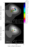 |
Fig. A.1 NOEMA data. The gray-scale map reproduces the 1.37 mm continuum emission, plotting values in the range 10–35 mJy beam−1. The colored dots give the (Gaussian-fitted) positions of the channel emission peaks for the CH3 CN JK = 12K–11K (K = 3–6) (upper panel) and HC3N J = 24–23 (lower panel) lines; the color denotes the channel VLSR. The yellow contours show the JVLA A-Array continuum at 1.3 cm (Moscadelli et al. 2016), showing levels at 70, 80, and 90% of the peak emission of 0.50 mJy beam−1. |
Appendix B Momentum of the molecular outflow
The momentum, Pout, of the molecular outflow can be calculated using the 13CO J = 2–1 and SO JN = 65–54 emission lines, which at sufficiently high absolute LOS velocities (|VLSR − Vsys|≥ 3 km s−1; see Figs. 3 and 4) mainly trace the outflowing gas. In the limit of optically thin emission, we can use the following expressions (see, for instance, Goldsmith & Langer 1999, Eq. (10)):

where iout is the inclination angle of the outflow with respect to the LOS, the index k considers separately the two, blue- (k = 1) and red-shifted (k = 2), outflow lobes, the sum in n extends over the velocity channels (n1,k ≤ n ≤ n2,k) of each lobe, and j runs over all the J pixels of the maps shown in Figs. 3 and 4. In Eq. (B.1), In,j and Vn are, respectively, the map intensity and VLSR at pixel j for channel n, V⋆ (≈ −6.4 km s−1, see Sect. 4.2.2) is the VLSR of YSO-1, δV (0.5 km s−1) is the channel width, d the distance (1.63 kpc) and δΩ the solid angle of the pixel. In Eq. (B.2), Bmax and Bmin are the FWHM sizes of the map beam along the major and minor axes, respectively, Tex the excitation temperature of the line, Eu, gu and Aul the energy and the statistical weight of the upper level and the spontaneous emission coefficient, respectively, of the transition, Zmol(Tex) the molecular partition function, Xmol the molecular abundance with respect to the H2 molecule, μ = 2.8 the mean molecular weight, mH the mass of the hydrogen atom, h the Planck constant, and c the speed oflight.
Table B.1 reports the parameters of the 13CO J = 2–1 and SO JN = 65–54 transitions, recovered from databases of molecular spectroscopy. Assuming LTE conditions, the Tex of the two lines can be approximated with the gas kinetic temperature. A lower limit is the value of ≈66 K, averaged over the full extent of the cluster, derived by Beuther et al. (2018, see Table 3) by fitting the IRAM 30 m H2 CO data at an angular resolution of 11.′′8 with XCLASS; an upper limit is the maximum temperature of ≈200 K toward core 1 from the XCLASS fit of the CH3CN JK = 12K–11K (K = 0–6) lines (see Fig. 11). We then use for both lines Tex = 100 K, which should be accurate to within a factor of 2. We verified that the error on the outflow momentum owing to this uncertainty on Tex is less than a factor of 2. By fitting the emission of the two lines and the dust continuum with XCLASS, and assuming the same dust absorption coefficient and gas-to-dust mass ratio of Sect. 4.1.2, we estimated the abundance ratios (with respect to H2) of the 13CO and SO molecules to be 2 × 10⁻⁶ and 10−8, respectively. Employing asingle line for each molecular species does not allow us to correct for optical depth effects, which can be significant in particular for the more abundant 13CO. The H2 column density is derived from NOEMA-only data, so due to potential missing flux (by about a factor of 2 for IRAS 21078+5211, Beuther et al. 2018, see Table 3), it is likely a lower limit as well. Based on our experience with the CORE data, we judge that these estimates of the abundance ratios should be correct within a factor of 3.
The VLSR ranges [V1,k, V2,k] (where V1,k and V2,k are the velocities of the channels n1,k and n2,k, respectively) for the blue- (k = 1) and red-shifted (k = 2), outflow lobes (see Table B.1) are selected in such a way to include only the channels where the 13CO J = 2–1 and SO JN = 65–54 emissions are detected with a high signal-to-noise ratio (see Figs. 3 and 4; the channel at VLSR = −28.1 km s−1 of the SO JN = 65–54 line is excluded because it is too noisy).
Summing over the two outflow lobes, we derive a momentum for the molecular outflow of ~17 and ~82 M⊙ km s−1 using the 13CO J = 2–1 and SO JN = 65–54 line, respectively. In the following, we adopt the intermediate value of Pout cos(iout) ~50 M⊙ km s−1, which, based on the above considerations, should be accurate to within an order of magnitude.
Parameters employed to calculate the momentum of the molecular outflow.
References
- Ageorges, N., Seifert, W., Jütte, M., et al. 2010, SPIE Conf. Ser., 7735, 77351L [Google Scholar]
- Ahmadi, A., Beuther, H., Mottram, J. C., et al. 2018, A&A, 618, A46 [NASA ADS] [CrossRef] [EDP Sciences] [Google Scholar]
- Anglada, G., Rodríguez, L. F., & Carrasco-González, C. 2018, A&ARv, 26, 3 [NASA ADS] [CrossRef] [Google Scholar]
- Bacciotti, F., Ray, T. P., Mundt, R., Eislöffel, J., & Solf, J. 2002, ApJ, 576, 222 [NASA ADS] [CrossRef] [Google Scholar]
- Barklem, P. S., & Collet, R. 2016, A&A, 588, A96 [NASA ADS] [CrossRef] [EDP Sciences] [Google Scholar]
- Bell, A. R. 1978, MNRAS, 182, 147 [NASA ADS] [CrossRef] [Google Scholar]
- Beuther, H., Mottram, J. C., Ahmadi, A., et al. 2018, A&A, 617, A100 [NASA ADS] [CrossRef] [EDP Sciences] [Google Scholar]
- Blandford, R. D., & Payne, D. G. 1982, MNRAS, 199, 883 [NASA ADS] [CrossRef] [Google Scholar]
- Bonnell, I. A., Vine, S. G., & Bate, M. R. 2004, MNRAS, 349, 735 [NASA ADS] [CrossRef] [Google Scholar]
- Bosco, F., Beuther, H., Ahmadi, A., et al. 2019, A&A, 629, A10 [NASA ADS] [CrossRef] [EDP Sciences] [Google Scholar]
- Burns, R. A., Imai, H., Handa, T., et al. 2015, MNRAS, 453, 3163 [NASA ADS] [CrossRef] [Google Scholar]
- Cesaroni, R., Neri, R., Olmi, L., et al. 2005, A&A, 434, 1039 [NASA ADS] [CrossRef] [EDP Sciences] [Google Scholar]
- Cesaroni, R., Beuther, H., Ahmadi, A., et al. 2019, A&A, 627, A68 [EDP Sciences] [Google Scholar]
- Chen, H.-R. V., Zhang, Q., Wright, M. C. H., et al. 2019, ApJ, 875, 24 [NASA ADS] [CrossRef] [Google Scholar]
- Clark, B. G. 1980, A&A, 89, 377 [NASA ADS] [Google Scholar]
- Coffey, D., Bacciotti, F., Woitas, J., Ray, T. P., & Eislöffel, J. 2004, ApJ, 604, 758 [NASA ADS] [CrossRef] [Google Scholar]
- Csengeri, T., Bontemps, S., Wyrowski, F., et al. 2017, A&A, 600, L10 [NASA ADS] [CrossRef] [EDP Sciences] [Google Scholar]
- Davies, B., Hoare, M. G., Lumsden, S. L., et al. 2011, MNRAS, 416, 972 [NASA ADS] [CrossRef] [Google Scholar]
- Di Francesco, J., Johnstone, D., Kirk, H., MacKenzie, T., & Ledwosinska, E. 2008, ApJS, 175, 277 [NASA ADS] [CrossRef] [Google Scholar]
- Draine, B. T. 2011, Physics of the Interstellar and Intergalactic Medium (Princeton: Princeton University Press) [Google Scholar]
- Egan, M. P., Price, S. D., & Kraemer, K. E. 2003, BAAS, 35, 1301 [NASA ADS] [Google Scholar]
- Esposito, S., Riccardi, A., Pinna, E., et al. 2012, in SPIE Conf. Ser., 8447, 84470U [Google Scholar]
- Federrath, C. 2015, MNRAS, 450, 4035 [NASA ADS] [CrossRef] [Google Scholar]
- Fendt, C., & Zinnecker, H. 1998, A&A, 334, 750 [NASA ADS] [Google Scholar]
- Gieser, C., Semenov, D., Beuther, H., et al. 2019, A&A, 631, A142 [NASA ADS] [CrossRef] [EDP Sciences] [Google Scholar]
- Gieser, C., Beuther, H., Semenov, D., et al. 2021, A&A, in press, https://doi.org/10.1051/0004-6361/202039670 [Google Scholar]
- Goddi, C., Humphreys, E. M. L., Greenhill, L. J., Chandler, C. J., & Matthews, L. D. 2011, ApJ, 728, 15 [NASA ADS] [CrossRef] [Google Scholar]
- Goldsmith, P. F., & Langer, W. D. 1999, ApJ, 517, 209 [Google Scholar]
- Gómez-Ruiz, A. I., Codella, C., Lefloch, B., et al. 2015, MNRAS, 446, 3346 [NASA ADS] [CrossRef] [Google Scholar]
- Hennebelle, P., Lee, Y.-N., & Chabrier, G. 2019, ApJ, 883, 140 [Google Scholar]
- Hirano, S., & Machida, M. N. 2019, MNRAS, 485, 4667 [NASA ADS] [CrossRef] [Google Scholar]
- Hoare, M. G., Lumsden, S. L., Oudmaijer, R. D., et al. 2005, IAU Symp., 227, 370 [Google Scholar]
- Klessen, R. S., & Glover, S. C. O. 2016, Saas-Fee Advanced Course, 43, 85 [Google Scholar]
- Kobayashi, H., Sasao, T., Kawaguchi, N., et al. 2003, ASP Conf. Ser., 306, P48 [Google Scholar]
- Kölligan, A., & Kuiper, R. 2018, A&A, 620, A182 [NASA ADS] [CrossRef] [EDP Sciences] [Google Scholar]
- Lampton, M., Margon, B., & Bowyer, S. 1976, ApJ, 208, 177 [NASA ADS] [CrossRef] [Google Scholar]
- Longmore, S. N., Kruijssen, J. M. D., Bastian, N., et al. 2014, Protostars and Planets VI, eds. H. Beuther, R. S. Klessen, C. P. Dullemond, & T. Henning (Tucson, AZ: University of Arizona Press), 291 [Google Scholar]
- Lu, X., Zhang, Q., Liu, H. B., et al. 2018, ApJ, 855, 9 [NASA ADS] [CrossRef] [Google Scholar]
- Lumsden, S. L., Hoare, M. G., Urquhart, J. S., et al. 2013, ApJS, 208, 11 [NASA ADS] [CrossRef] [Google Scholar]
- Machida, M. N., Hirano, S., & Kitta, H. 2020, MNRAS, 491, 2180 [Google Scholar]
- Masson, C. R., & Chernin, L. M. 1993, ApJ, 414, 230 [NASA ADS] [CrossRef] [Google Scholar]
- Maud, L. T., Moore, T. J. T., Lumsden, S. L., et al. 2015, MNRAS, 453, 645 [NASA ADS] [CrossRef] [Google Scholar]
- McKee, C. F.,& Tan, J. C. 2003, ApJ, 585, 850 [NASA ADS] [CrossRef] [MathSciNet] [Google Scholar]
- Molinari, S., Brand, J., Cesaroni, R., & Palla, F. 1996, A&A, 308, 573 [NASA ADS] [Google Scholar]
- Molinari, S., Swinyard, B., Bally, J., et al. 2010a, PASP, 122, 314 [NASA ADS] [CrossRef] [Google Scholar]
- Molinari, S., Swinyard, B., Bally, J., et al. 2010b, A&A, 518, L100 [NASA ADS] [CrossRef] [EDP Sciences] [Google Scholar]
- Möller, T., Endres, C., & Schilke, P. 2017, A&A, 598, A7 [NASA ADS] [CrossRef] [EDP Sciences] [Google Scholar]
- Moscadelli, L., Sánchez-Monge, Á., Goddi, C., et al. 2016, A&A, 585, A71 [NASA ADS] [CrossRef] [EDP Sciences] [Google Scholar]
- Moscadelli, L., Sanna, A., Goddi, C., et al. 2019, A&A, 631, A74 [NASA ADS] [CrossRef] [EDP Sciences] [Google Scholar]
- Moscadelli, L., Sanna, A., Goddi, C., et al. 2020, A&A, 635, A118 [EDP Sciences] [Google Scholar]
- Mottram, J. C., Beuther, H., Ahmadi, A., et al. 2020, A&A, 636, A118 [EDP Sciences] [Google Scholar]
- Müller, H. S. P., Thorwirth, S., Roth, D. A., & Winnewisser, G. 2001, A&A, 370, L49 [NASA ADS] [CrossRef] [EDP Sciences] [Google Scholar]
- Müller, H. S. P., Schlöder, F., Stutzki, J., & Winnewisser, G. 2005, J. Mol. Struct., 742, 215 [Google Scholar]
- Myers, P. C. 2009, ApJ, 700, 1609 [NASA ADS] [CrossRef] [EDP Sciences] [Google Scholar]
- Neugebauer, G., Habing, H. J., van Duinen, R., et al. 1984, ApJ, 278, L1 [Google Scholar]
- Neupane, S., Garay, G., Contreras, Y., Guzmán, A. E., & Rodríguez, L. F. 2020, ApJ, 890, 76 [Google Scholar]
- Ossenkopf, V., & Henning, T. 1994, A&A, 291, 943 [NASA ADS] [Google Scholar]
- Padoan, P., Pan, L., Juvela, M., Haugbølle, T., & Nordlund, Å. 2020, ApJ, 900, 82 [Google Scholar]
- Palla, F., & Stahler, S. W. 1993, ApJ, 418, 414 [NASA ADS] [CrossRef] [Google Scholar]
- Parker, N. D., Padman, R., & Scott, P. F. 1991, MNRAS, 252, 442 [NASA ADS] [CrossRef] [Google Scholar]
- Pickett, H. M., Poynter, R. L., Cohen, E. A., et al. 1998, J. Quant. Spectr. Rad. Transf., 60, 883 [Google Scholar]
- Podio, L., Codella, C., Gueth, F., et al. 2015, A&A, 581, A85 [NASA ADS] [CrossRef] [EDP Sciences] [Google Scholar]
- Pudritz, R. E., & Ray, T. P. 2019, Front. Astron. Space Sci., 6, 54 [CrossRef] [Google Scholar]
- Pudritz, R. E., Ouyed, R., Fendt, C., & Brandenburg, A. 2007, Protostars and Planets V, eds. B. Reipurth, D. Jewitt, & K. Keil (Tucson, AZ: University of Arizoan Press), 277 [Google Scholar]
- Ragan, S. E., Heitsch, F., Bergin, E. A., & Wilner, D. 2012, ApJ, 746, 174 [NASA ADS] [CrossRef] [Google Scholar]
- Ray, T., Dougados, C., Bacciotti, F., Eislöffel, J., & Chrysostomou, A. 2007, Protostars and Planets V, eds. B. Reipurth, D. Jewitt, & K. Keil (Tucson, AZ: University of Arizona Press), 231 [Google Scholar]
- Reid, M. J., Schneps, M. H., Moran, J. M., et al. 1988, ApJ, 330, 809 [NASA ADS] [CrossRef] [Google Scholar]
- Reid, M. J., Menten, K. M., Brunthaler, A., et al. 2009, ApJ, 693, 397 [NASA ADS] [CrossRef] [Google Scholar]
- Reid, M. J., Menten, K. M., Brunthaler, A., et al. 2014, ApJ, 783, 130 [Google Scholar]
- Sanhueza, P., Contreras, Y., Wu, B., et al. 2019, ApJ, 886, 102 [NASA ADS] [CrossRef] [Google Scholar]
- Sanna, A., Moscadelli, L., Goddi, C., Krishnan, V., & Massi, F. 2018, A&A, 619, A107 [NASA ADS] [CrossRef] [EDP Sciences] [Google Scholar]
- Sanna, A., Moscadelli, L., Goddi, C., et al. 2019, A&A, 623, L3 [NASA ADS] [CrossRef] [EDP Sciences] [Google Scholar]
- Schwörer, A., Sánchez-Monge, Á., Schilke, P., et al. 2019, A&A, 628, A6 [NASA ADS] [CrossRef] [EDP Sciences] [Google Scholar]
- Seifert, W., Ageorges, N., Lehmitz, M., et al. 2010, SPIE Conf. Ser., 7735, 77357W [Google Scholar]
- Shepherd, D. S., Yu, K. C., Bally, J., & Testi, L. 2000, ApJ, 535, 833 [Google Scholar]
- Smith, R. J., Shetty, R., Beuther, H., Klessen, R. S., & Bonnell, I. A. 2013, ApJ, 771, 24 [NASA ADS] [CrossRef] [Google Scholar]
- Staff, J., Koning, N., Ouyed, R., & Pudritz, R. 2014, Eur. Phys. J. Web Conf., 64, 05006 [Google Scholar]
- Staff, J. E., Koning, N., Ouyed, R., Thompson, A., & Pudritz, R. E. 2015, MNRAS, 446, 3975 [NASA ADS] [CrossRef] [Google Scholar]
- Staff, J. E., Tanaka, K. E. I., & Tan, J. C. 2019, ApJ, 882, 123 [CrossRef] [Google Scholar]
- Steer, D. G., Dewdney, P. E., & Ito, M. R. 1984, A&A, 137, 159 [NASA ADS] [Google Scholar]
- Terquem, C., Eislöffel, J., Papaloizou, J. C. B., & Nelson, R. P. 1999, ApJ, 512, L131 [NASA ADS] [CrossRef] [EDP Sciences] [Google Scholar]
- Testi, L., Palla, F., & Natta, A. 1999, A&A, 342, 515 [NASA ADS] [Google Scholar]
- Tobin, J. J., Hartmann, L., Bergin, E., et al. 2012, ApJ, 748, 16 [Google Scholar]
- Treviño-Morales, S. P., Fuente, A., Sánchez-Monge, Á., et al. 2019, A&A, 629, A81 [NASA ADS] [CrossRef] [EDP Sciences] [Google Scholar]
- Tsukamoto, Y., Okuzumi, S., Iwasaki, K., Machida, M. N., & Inutsuka, S. 2018, ApJ, 868, 22 [NASA ADS] [CrossRef] [Google Scholar]
- Vázquez-Semadeni, E., Palau, A., Ballesteros-Paredes, J., Gómez, G. C., & Zamora-Avilés, M. 2019, MNRAS, 490, 3061 [Google Scholar]
- Wang, K., Zhang, Q., Testi, L., et al. 2014, MNRAS, 439, 3275 [NASA ADS] [CrossRef] [Google Scholar]
- Winter, A. J., Booth, R. A., & Clarke, C. J. 2018, MNRAS, 479, 5522 [Google Scholar]
- Wright, E. L., Eisenhardt, P. R. M., Mainzer, A. K., et al. 2010, AJ, 140, 1868 [Google Scholar]
- Xu, Y., Li, J. J., Reid, M. J., et al. 2013, ApJ, 769, 15 [NASA ADS] [CrossRef] [Google Scholar]
The Bar and Spiral Structure Legacy (BeSSeL) survey is a VLBA key project, whose main goal is to derive the structure and kinematics of the Milky Way by measuring accurate positions, distances (via trigonometric parallaxes), and proper motions of methanol and water masers in hundreds of high-mass star-forming regions distributed over the Galactic disk (Reid et al. 2014).
Neither Herschel infrared Galactic Plane Survey (Hi-GAL; Molinari et al. 2010b,a) nor red MSX source (RMS; Hoare et al. 2005; Lumsden et al. 2013) observations are available for IRAS 21078+5211.
All Tables
All Figures
|
Fig. 1 Upper panel: NOEMA 1.37 mm continuum emission (color map) of IRAS 21078+5211. The white contours correspond to levels ranging from 3σ (σ = 0.5 mJy beam−1) to the peak intensity of 35 mJy beam−1, in steps of 7σ. The little black crosses indicate the positions of the seven strongest 1.37 mm peaks labeled as in Beuther et al. (2018, see Table 5), with label numbers ordered in intensity. The restoring beam of the 1.37 mm continuum map is shown in the lower left corner. Lower panel: Wide-field Infrared Survey Explorer (WISE) 4.6 μm image (color map, Wright et al. 2010) toward IRAS 21078+5211. The white contours represent the SCUBA 850 μm continuum (Di Francesco et al. 2008), showing 10 levels increasing logarithmically from 7σ (σ = 0.1 Jy beam−1) to 11.4 Jy beam−1. The magenta rectangle delimits the region plotted in the upper panel. |
| In the text | |
|
Fig. 2 IRAM 30 m data. Intensity-weighted velocity (color map) of the C18O J = 2–1 (upper panel), 13CO J = 2–1 (middle panel), and H2CO |
| In the text | |
|
Fig. 3 Merged NOEMA–IRAM 30 m data. Each panel presents the emission of the 13CO J = 2–1 line (color map) in a different velocity channel. In the upper right corner of the panel, the channel VLSR (in kilometer per second) and the range of plotted intensity (in square parentheses in milliJansky per beam) are reported. The red boxes and ticks identify the panels corresponding to the central velocities, that is |VLSR − Vsys| < 3 km s−1. The white crosses mark the positions of the seven strongest peaks of the 1.37 mm continuum emission. At the central velocities, the black dashed line gives the major axis of the 1.37 mm core cluster. |
| In the text | |
|
Fig. 4 Merged NOEMA–IRAM 30 m data. Each panel presents the emission of the SO JN = 65–54 line (color map) in a different velocity channel. In the upper right corner of the panel, the channel VLSR (in kilometer per second) and the range of plotted intensity (in square parentheses in milliJansky per beam) are reported. The red boxes and ticks identify the panels corresponding to the central velocities, that is |VLSR − Vsys| < 3 km s−1. The white crosses mark the positions of the seven strongest peaks of the 1.37 mm continuum emission. |
| In the text | |
|
Fig. 5 Upper panel: NOEMA data. Velocity-integrated intensity (color map) of the CH3 CN JK = 123–113 line. The 1.37 mm continuum emission is represented with black contours, showing seven levels increasing logarithmically from 11 to 35 mJy beam−1. The positions of the three strongest peaks of the 1.37 mm continuum emission are indicated, using the same labels as in Beuther et al. (2018, see Table 5). The restoring beams of the CH3 CN JK = 123–113 line and 1.37 mm continuum maps are shown in the lower right and left corners, respectively. Lower panel: the blue and red contours reproduce the emission of the SO JN = 65–54 line integrated over the velocity ranges [−22,−13] and [−1, 5] km s−1, respectively. The plotted levels are from 0.03 to 2.5 Jy beam−1, in steps of 0.27 Jy beam−1, and from 0.6 to 2.2 Jy beam−1, in steps of 0.37 Jy beam−1, for the blue- and red-shifted SO emission, respectively. The magenta contours give the JVLA A-Array continuum at 5 cm (Moscadelli et al. 2016), showing levels at 40, 50, and 90% of the peak emission of 95 μJy beam−1: the magenta dashed line connects the two strongest (nearby, but resolved) 5 cm peaks. The two black dashed lines delimit the viewing angle of the blue-shifted emission of the SO JN = 65–54 line from the NE 5 cm peak (aligned in position with core 1, see Sect. 3.1). The black contours have the same meaning as in the upper panel. |
| In the text | |
|
Fig. 6 Beam-averaged spectrum (black line) of the CH3CN JK = 12K–11K (K = 0–8) line emissiontoward the 1.37 mm continuum peak. The positions of the K = 0–8 lines are indicated. The fits (red histograms) of the K = 0–6 lines performed with XCLASS are also shown. |
| In the text | |
|
Fig. 7 NOEMA data. The color map reproduces the column density (upper panel) and the velocity (lower panel) of the CH3 CN emission determined by fitting with XCLASS the CH3CN JK = 12K–11K (K = 0–6) lines (including the CH3 13CN isotopologs), simultaneously. The plotted regions correspond to the areas in which the 1.37 mm continuum emission is higher than 13 and 16 mJy beam−1 for the column density and velocity plots, respectively. The 1.37 mm continuum emission is represented with black contours, showing six levels increasing logarithmically from 13 to 35 mJy beam−1: the positions of the three strongest 1.37 mm peaks are denoted using the same labels as in Beuther et al. (2018, see Table 5). The restoring beams of the 1.37 mm continuum and CH3 CN maps are shown in the lower left corner of the upper panel and lower right corner of the lower panel, respectively. |
| In the text | |
|
Fig. 8 NOEMA data. Upper panels: the color maps reproduce the emission of the CH3 CN JK = 125–115 (left) and CH2CO |
| In the text | |
|
Fig. 9 Comparison of CORE, POETS and LBT observations. Upper panel: the gray-scale map reproduces the H2 2.12 μm emission observed with LBT toward IRAS 21078+5211. Referring to Fig. 5, lower panel, the blue and red contours have the same meaning, and the yellow contours replace the magenta contours for the JVLA 5 cm continuum. The magenta dashed, white dotted, and cyan dashed lines connect the main 5 cm peak with the secondary (nearby) 5 cm peak, the weak 5 cm spur to NE, and the bow shock traced by the LBT H2 2.12 μm emissionto SW, respectively. The white dashed box delimits the region plotted in the lower panel. Lower panel: adaptive-optics assisted LBT observations of the H2 2.12 μm emission (gray-scale map): the cyan dashed line has the same meaning as in the upper panel. |
| In the text | |
|
Fig. 10 NOEMA data. Upper panel: the gray-scale map reproduces the 1.37 mm continuum emission, plotting values in the range 10–35 mJy beam−1. The colored dots give the (Gaussian-fitted) positions of the channel emission peaks for the CH3 CN JK = 12K–11K (K = 3–6) and HC3N J = 24–23 lines; the colors denote the channel VLSR. The colored contours indicate the half-peak level for the CH3CN JK = 123-113 emission in individual channels. The yellow contours show the JVLA A-Array continuum at 1.3 cm (Moscadelli et al. 2016), showing levels at 70, 80, and 90% of the peak emission of 0.50 mJy beam−1. Lower panel: the gray-scale map, yellow contours, and colored dots have the same meaning as in the upper panel. Only the channel emission peaks at the extreme blue- and red-shifted velocities (reported in the lower right corner of the panel) are shown. The white continuous and dashed lines indicate the best-fit major axis of the distribution of the peaks and the corresponding fit uncertainty, respectively. |
| In the text | |
|
Fig. 11 NOEMA data. The color map shows the distribution of the rotational temperature derived by fitting with XCLASS the emission of the CH3CN JK = 12K–11K (K = 0–6) lines (including the CH3 13CN isotopologs). The plotted region corresponds to the area in which the 1.37 mm continuum emission is higher than 16 mJy beam−1. The black contours reproduce the 1.37 mm continuum, showing the same levels as in Fig. 7: the positions of the three strongest 1.37 mm peaks are indicated using the same labels as in Beuther et al. (2018, see Table 5). The restoring beam of the CH3 CN maps is shown in the lower right corner of the panel. |
| In the text | |
|
Fig. 12 POETS water maser observations. Upper panel: colored dots and arrows give absolute positions and proper motions of the 22 GHz water masers determined with VLBI observations (Moscadelli et al. 2016); colors denote the maser VLSR. The dot area scales logarithmically with the maser intensity. The black contours indicate the JVLA A-Array continuum at 1.3 cm (Moscadelli et al. 2016), showing levels from 10 to 90% of the peak emission of 0.50 mJy beam−1 in steps of 10%. Lower panel: colored dots and black contours have the same meaning as in the upper panel. Colored cones are employed to visualize the maser 3D velocities, representing the inclination with respect to the LOS through the ellipticity of the cone basis and the uncertainty in the direction by means of the cone aperture. |
| In the text | |
|
Fig. 13 χ2 values from the Keplerian fit (see Eq. (1)) vs. the free parameter M⋆ sin 2(irot). The horizontal black dashed line indicates the value |
| In the text | |
|
Fig. 14 Maser positions projected perpendicular to the jet axis, Rper, vs. corresponding LOS velocities, VLOS, for the masers with VLOS ≥ −20 km s−1. Colored error bars are used to indicate values and associated errors; the colors represent the distance from YSO-1 projected along the jet axis, Raxi, as coded in the wedge on the right-hand side of the panel. The black dashed line shows the linear fit to the plotted values. |
| In the text | |
|
Fig. 15 Components Vaxi vs. VΦ (see definitions in Sect. 4.3) for the 3D maser velocities shown in Fig. 12. Colored error bars are used to indicate values and associated errors; the colors represent the distance from YSO-1 projected along the jet axis, Raxi, as coded in the wedge on the right-hand side of the panel. The black dashed line shows the linear fit to the subset of points within the region delimited by the horizontal and vertical black dotted lines, corresponding to VΦ ≤ 20 km s−1 and Vaxi ≥ 5 km s−1. |
| In the text | |
|
Fig. A.1 NOEMA data. The gray-scale map reproduces the 1.37 mm continuum emission, plotting values in the range 10–35 mJy beam−1. The colored dots give the (Gaussian-fitted) positions of the channel emission peaks for the CH3 CN JK = 12K–11K (K = 3–6) (upper panel) and HC3N J = 24–23 (lower panel) lines; the color denotes the channel VLSR. The yellow contours show the JVLA A-Array continuum at 1.3 cm (Moscadelli et al. 2016), showing levels at 70, 80, and 90% of the peak emission of 0.50 mJy beam−1. |
| In the text | |
Current usage metrics show cumulative count of Article Views (full-text article views including HTML views, PDF and ePub downloads, according to the available data) and Abstracts Views on Vision4Press platform.
Data correspond to usage on the plateform after 2015. The current usage metrics is available 48-96 hours after online publication and is updated daily on week days.
Initial download of the metrics may take a while.