| Issue |
A&A
Volume 645, January 2021
|
|
|---|---|---|
| Article Number | A21 | |
| Number of page(s) | 24 | |
| Section | Extragalactic astronomy | |
| DOI | https://doi.org/10.1051/0004-6361/202038256 | |
| Published online | 22 December 2020 | |
Multiphase feedback processes in the Sy2 galaxy NGC 5643
1
Department of Physics, University of Oxford, Oxford OX1 3RH, UK
e-mail: igbernete@gmail.com
2
Centro de Astrobiología, CSIC-INTA, ESAC Campus, 28692 Villanueva de la Cañada, Madrid, Spain
3
Observatorio Astronómico Nacional (OAN-IGN)-Observatorio de Madrid, Alfonso XII, 3, 28014 Madrid, Spain
4
Centro de Astrobiología, CSIC-INTA, Carretera de Torrejón a Ajalvir, 28880 Torrejón de Ardoz, Madrid, Spain
5
Instituto de Astrofísica de Canarias, Calle vía Láctea, s/n, 38205 La Laguna, Tenerife, Spain
6
Departamento de Astrofísica, Universidad de La Laguna, 38205 La Laguna, Tenerife, Spain
7
Instituto de Física de Cantabria (CSIC-UC), Avenida de los Castros, 39005 Santander, Spain
8
Instituto de Radioastronomía y Astrofísica (IRyA-UNAM), 3-72 (Xangari), 8701 Morelia, Mexico
9
Department of Physics & Astronomy, University of Alaska Anchorage, Anchorage, AK 99508-4664, USA
10
Núcleo de Astronomía de la Facultad de Ingeniería, Universidad Diego Portales, Av. Ejército Libertador 441, Santiago, Chile
11
Kavli Institute for Astronomy and Astrophysics, Peking University, Beijing 100871, PR China
12
George Mason University, Department of Physics & Astronomy, MS 3F3, 4400 University Drive, Fairfax, VA 22030, USA
Received:
24
April
2020
Accepted:
11
September
2020
We study the multiphase feedback processes in the central ∼3 kpc of the barred Seyfert 2 galaxy NGC 5643. We used observations of the cold molecular gas (ALMA CO(2−1) transition) and ionized gas (MUSE IFU optical emission lines). We studied different regions along the outflow zone, which extends out to ∼2.3 kpc in the same direction (east-west) as the radio jet, as well as nuclear and circumnuclear regions in the host galaxy disk. The CO(2−1) line profiles of regions in the outflow and spiral arms show two or more different velocity components: one associated with the host galaxy rotation, and the others with out- or inflowing material. In the outflow region, the [O III]λ5007 Å emission lines have two or more components: the narrow component traces rotation of the gas in the disk, and the others are related to the ionized outflow. The deprojected outflowing velocities of the cold molecular gas (median Vcentral ∼ 189 km s−1) are generally lower than those of the outflowing ionized gas, which reach deprojected velocities of up to 750 km s−1 close to the active galactic nucleus (AGN), and their spatial profiles follow those of the ionized phase. This suggests that the outflowing molecular gas in the galaxy disk is being entrained by the AGN wind. We derive molecular and ionized outflow masses of ∼5.2 × 10⁷ M⊙ (αCOGalactic) and 8.5 × 10⁴ M⊙ and molecular and ionized outflow mass rates of ∼51 M⊙ yr−1 (αCOGalactic) and 0.14 M⊙ yr−1, respectively. This means that the molecular phase dominates the outflow mass and outflow mass rate, while the kinetic power and momentum of the outflow are similar in both phases. However, the wind momentum loads (Ṗout/ṖAGN) for the molecular and ionized outflow phases are ∼27−5 (αCOGalactic and αCOULIRGs) and < 1, which suggests that the molecular phase is not momentum conserving, but the ionized phase most certainly is. The molecular gas content (Meast ∼ 1.5 × 10⁷ M⊙; αCOGalactic) of the eastern spiral arm is approximately 50−70% of the content of the western one. We interpret this as destruction or clearing of the molecular gas produced by the AGN wind impacting in the eastern side of the host galaxy (negative feedback process). The increase in molecular phase momentum implies that part of the kinetic energy from the AGN wind is transmitted to the molecular outflow. This suggests that in Seyfert-like AGN such as NGC 5643, the radiative or quasar and the kinetic or radio AGN feedback modes coexist and may shape the host galaxies even at kiloparsec scales through both positive and (mild) negative feedback.
Key words: galaxies: active / galaxies: Seyfert / galaxies: individual: NGC 5643 / Galaxy: kinematics and dynamics / submillimeter: galaxies
© ESO 2020
1. Introduction
The impact of the energy released by active galactic nuclei (AGN) in the form of radiation and/or mechanical outflows in the host galaxy interstellar medium has been proposed as a key mechanism that is responsible for regulating star formation in galaxies. In cosmological simulations, AGN feedback is needed to reproduce the observed number of massive galaxies through the quenching of star formation (e.g., Bower et al. 2006; Croton et al. 2006; Bongiorno et al. 2016), although other less significant heating sources such as supernovae might also play a role (e.g., Silk & Mamon 2012). Additionally, recent studies found observational evidence of positive AGN feedback (e.g., Klamer et al. 2004; Norris 2009; Cresci et al. 2015; Maiolino et al. 2017; Shin et al. 2019), which favors compression and subsequent collapse in molecular gas, leading to an enhanced star formation rate.
AGN-driven winds appear to be ubiquitous in AGN, although their effect on the host galaxies is unclear. Moreover, AGN-driven outflows are detected in several phases from the extremely hot X-ray gas to the ionized phase to the cold molecular and neutral phases (e.g., Morganti 2017). It is thus essential to quantify the overall mass, momentum, and energy budget of each phase (e.g., Cicone et al. 2018). Recently, Fiore et al. (2017) compiled observations for a sample of 94 AGN with massive winds. They found a correlation between the molecular and ionized mass outflow rates and the AGN bolometric luminosity. These authors also reported that the outflow velocity is higher in the ionized phase, but that the mass outflow rate is dominated by the molecular phase, which becomes especially important at low to intermediate luminosities (Lbol = 1042–1045 erg s−1). However, this work employed a heterogeneous sample of AGN (0.003 < z < 6.4) that does not always have multiphase observations for the same galaxy. Except for a few nearby AGN, for instance, NGC 1068 by García-Burillo et al. (2014, 2019) and NGC 5728 by Shimizu et al. (2019), there is a lack of detailed multiphase studies using various regions within the same source. Nearby Seyfert galaxies are intermediate-luminosity AGN (LX = 1042–1044 erg s−1) and afford the necessary physical resolution to study the multiphase outflow properties in different regions.
This pilot study aims to investigate the AGN-driven outflow in the cold molecular and ionized gas phases of the Seyfert 2 galaxy NGC 5643. It is a barred Sy2 galaxy at ∼16.9 Mpc that is seen almost face-on (i ∼ −27°; de Vaucouleurs et al. 1976). It presents ionization cones detected in [O III]λ5007 Å (hereafter [O III]) and Hα at both sides of the nucleus with an elongated morphology along the east-west direction (e.g., Schmitt et al. 1994; Simpson et al. 1997). Using Very Large Telescope/Multi Unit Spectroscopic Explorer (VLT/MUSE) data, Cresci et al. (2015) showed that the kinematics of this double-sided ionization cone was consistent with outflows, based on the detection of a blueshifted asymmetric wing of the [O III] emission line. In the same orientation, VLA radio observations show emission at either side of this radio-quiet galaxy (log(L1.4 GHz) = 37.3 erg s−1; Meléndez et al. 2010), which is related to the emission of a radio jet (Morris et al. 1985; Leipski et al. 2006). This morphology is also approximately coincident with a large-scale stellar bar (Mulchaey et al. 1997). We refer to Cresci et al. (2015) for further details on the stellar and radio morphology. The nuclear H2 1−0S(1) velocity field also shows evidence of noncircular motions in the hot molecular gas (Davies et al. 2014). Recently, Alonso-Herrero et al. (2018) presented high angular resolution CO(2−1) line and 232 GHz continuum observations obtained with ALMA. The authors showed that in the outflow region, the CO(2−1) emission has generally two kinematic components, one associated with rotation in the disk of the galaxy, and another due to the interaction of the AGN outflow with the molecular gas. Additionally, there is observational evidence of positive AGN feedback in this galaxy (Cresci et al. 2015).
The paper is organized as follows. Section 2 describes the observations and data compilation. The spectral analysis is presented in Sect. 3. In Sect. 4 we compare the molecular and ionized gas distribution and kinematics. In Sect. 5 we study the connection between the molecular and ionized gas phases, and in Sect. 6 we compare observational data for the ionized wind with an analytic model of the outflow wind. Finally, we summarize the main conclusions in Sect. 7.
2. Observations
2.1. ALMA data
NGC 5643 was observed in Band 6 using the 12 m ALMA array with a compact (baselines between 15 and 492 m) and an extended configuration (baselines between 17 and 3700 m). The data were obtained as part of the project 2016.1.00254.S (PI: A. Alonso-Herrero), and the on-source integration times were 11 and 36 min for the compact and extended configuration, respectively. The original field of view (FoV) of these data is ∼40″ × 20″ (∼3.3 kpc × 1.6 kpc) with a spectral resolution of 15 km s−1 and an angular resolution of 0.26″ × 0.17″ at a beam position angle (PAbeam) of −69.6°. The fully reduced and clean CO(2−1) natural weight data cube was taken from Alonso-Herrero et al. (2018). Figure 1 shows the central ∼2.9 kpc × 1.6 kpc FoV in which the outflow region dominates.
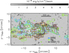 |
Fig. 1. ALMA CO(2−1) integrated intensity map of NGC 5643 in gray scale, produced from the natural-weight data cube on a linear scale. The black contours are the CO(2−1) emission on a logarithmic scale. The first contour lies at 8σ and the last contour at 8.7 × 10⁻¹⁸ erg s−1 cm2 beam−1. Filled blue and green contours are the MUSE [O III]λ5007 Å and Hα emission maps (see Sect. 4), respectively. Red and orange regions correspond to the outflow and nuclear spiral selected zones, respectively. North is up and east is left, and offsets are measured relative to the AGN. |
2.2. Archival VLT/MUSE integral field spectroscopy
Optical integral field spectroscopy of NGC 5643 was taken using the Multi Unit Spectroscopic Explorer (MUSE, Bacon et al. 2010) on the 8.2 m Very Large Telescope (VLT). These data were observed as part of the program 095.B-0532(A) (PI: Carollo). This dataset has been presented in Erroz-Ferrer et al. (2019). We downloaded the fully reduced and calibrated science data cube from the ESO data archive1. We remark that this MUSE data cube, first presented in Alonso-Herrero et al. (2018), was observed under significantly better seeing conditions than the one presented in Cresci et al. (2015), that is, ∼0.5″ versus ∼0.88″.
We focus on the emission line properties here, therefore we first subtracted the stellar continuum. We used STARLIGHT (Cid et al. 2005) to model the stellar continuum. This code combines library spectra (STELIB; Bruzual & Charlot 2003) of various ages and metallicities to reproduce the input spectrum. After the continuum subtraction, we fit the emission lines in each spaxel with amplitude-over-noise (AoN; the amplitude is the peak of the emission line) ratio is higher than 3 with Gaussian functions to derive the 2D maps of the brightest emission lines. Figure 1 shows the resulting [O III] map (blue image and blue contours) as well as the Hα emission (green contours).
2.3. Archival Spitzer data
We downloaded the fully reduced and extracted low-resolution mid-infrared (MIR) Spitzer/IRS (Houck et al. 2004) spectrum from the Cornell Atlas of Spitzer/IRS Source (CASSIS2; Lebouteiller et al. 2011). CASSIS uses an optimal extraction to achieve the best signal-to-noise ratio (S/N). The spectra were obtained using the staring mode and the low-resolution (R ∼ 60−120) IRS modules: the short-low (SL; 5.2−14.5 μm) and the long-low (LL; 14−38 μm). Finally, we only needed to apply a small offset to stitch the different modules together, taking the shorter wavelength module (SL2; 5.2−7.6 μm) as the basis. The latest has an associated a slit width of 3.7″.
3. Spectral analysis
3.1. Region selection
To study the kinematics of the ionized and molecular gas of NGC 5643, we selected 91 different regions. The outflow region as probed by the ionized gas emission extends out to 2.3 kpc in the east-west direction (as the radio emission), and in the north-south direction, approximately ∼800 pc to the east of the AGN and ∼500 pc to the west. The selected regions include bright CO(2−1) emission along the outflow zone, the borders of the outflow at either side of the galaxy (delimited by the [O III]/Hα bipolar nebulosity), and clumps with bright [O III] and Hα emission. These regions are marked with red boxes in Fig. 1. We also selected regions in the northern and southern parts of the nuclear and circumnuclear spiral structure seen in the CO(2−1) map, where the ionized gas emission is relatively weak. We marked these as orange boxes in Fig. 1. To extract the CO(2−1) and ionized gas emission from these regions, we chose 1.2″ × 1.2″ square apertures that are ∼2.5 times the MUSE full width at half maximum (FWHM) (Sect. 2).
Because the selected regions do not cover the ionized gas emission completely, we also extracted several larger slices (see Fig. A.1) along the outflow region. We defined slices with widths of 2.4″ and heights ranging from ∼6″ to ∼10″ depending on the extent of the [O III] emission. We used the location of the AGN as the reference, and then we applied the same offsets from the nucleus along the east-west direction. We constructed the slices by stacking spectra extracted with 1.2″ × 1.2″ square apertures and shifted them to a common rest-frame wavelength reference. We show the stacked [O III] and CO(2−1) spectra for each slice in Appendix A. This stacking technique greatly improves the S/N of the extracted spectra and thus allows us to detect weak kinematic components, which we use to derive the outflow properties in a uniform way (see Sect. 5).
3.2. CO(2−1) data
3.2.1. Rotating-disk model
Alonso-Herrero et al. (2018) showed that the ALMA CO(2−1) emission has different kinematic components (see also Figs. A.2 and A.3). The main component traces galaxy rotation. Following Alonso-Herrero et al. (2018), we fit a rotating-disk model to the CO(2−1) kinematics using the 3DBAROLO code (Di Teodoro & Fraternali 2015), but covering a larger FoV. We fixed the following parameters: inclination i = 35°, the position angle of the major kinematic axis PA = 320°, and the systemic velocity vsys = 1994 km s−1, as derived by Alonso-Herrero et al. (2018). 3DBAROLO produces the observed and best-fit model maps of the velocity-integrated intensity (zeroth moment), mean-velocity field (first moment), and velocity dispersion (second moment). Figure 2 (left panel) shows the resulting 3DBAROLO model for the central ∼10″ × 10″.
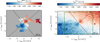 |
Fig. 2. Left panel: 3DBAROLO model of the mean velocity field of NGC 5643 using a rotating-disk model fitted to the natural-weight CO(2−1) data cube. Right panel: penalized pixel-fitting (pPXF) model of the stellar kinematics from the Ca II triplet lines using λ> 8000 Å MUSE data and pixels binned to S/N = 40. The solid and dashed black lines correspond to the kinematic minor and major axes, respectively. The green box in the right panel shows the FoV of the left panel. The northeastern (southwestern) region corresponds to the far (near) side. North is up and east is left, and offsets are measured relative to the AGN. |
3.2.2. Individual regions
For the majority of the selected regions, the CO(2−1) emission shows clearly deblended velocity components, except in regions near the AGN (see Figs. A.2 and A.3). We fit the various kinematic components to accurately measure their velocities and fluxes. Only when necessary (significant residuals of the fit; > 3 times the standard deviation) did we used two or three Gaussians for the fit. We used the PySpecKit code (Ginsburg & Mirocha 2011), which produces the best fit using the χ2 minimization.
In the region modeled by the rotating galaxy disk, the predicted velocity from the model and the brightest CO(2−1) component are in good agreement. Because we were unable to model the large-scale faint emission with BAROLO, we extrapolated the velocity field when possible to identify the galaxy disk emission line in the fitted kinematic components. In these cases, we considered the brightest feature as the galaxy disk component. Finally, we also verified that the velocities of the identified CO(2−1) rotation disk component agreed within the errors with those of the stellar kinematics (see Sect. 3.3.1 and the right panel of Fig. 2, and Appendix A). When we detected more than one kinematic component, the fainter components were assumed to trace noncircular motions (i.e., outflowing or inflowing material, see below).
3.2.3. Radial profile along the outflow
As discussed in Sect. 3.1, we also extracted several larger slices (see Fig. A.1) along the outflow region. Then, we fit all the emission lines with AoN > 3 for each slice spectrum using the same method as in Sect. 3.2.2 (see Figs. A.2 and A.3).
3.3. MUSE data
3.3.1. Stellar kinematics
We derived the stellar kinematics from the Ca II triplet lines using MUSE data at λ > 8000 Å and the penalized pixel-fitting (pPXF) method (Cappellari & Emsellem 2004; Cappellari 2017). To achieve the best spatial resolution possible with good S/N, we used the Voronoi binning algorithm (Cappellari & Copin 2003) for S/N = 40. The right panel of Fig. 2 shows that the S/N of the NGC 5643 MUSE data used in this work is high enough in the full ∼2.9 kpc × 1.6 kpc, and that the stellar kinematics agrees fairly well within the errors with the CO(2−1) rotating-disk model (see the left panel of Fig. 2).
3.3.2. Individual regions
To derive the kinematics of the ionized gas, and in particular, the properties of the outflow, we used the [O III] emission line. The [O III] line emission in all the selected regions shows complex and asymmetrical profiles. This suggests the presence of different kinematic components that require more than one Gaussian for the fit (see Figs. A.4 and A.5). To perform the emission line fitting, we used the PySpecKit code as in Sect. 3.2. Then, after the stellar continuum subtraction, we fit the [O III] doublet emission lines (when the [O III]λ5007 Å emission line has AoN > 3) simultaneously with the same velocity and widths, which are always larger than the instrumental one (i.e., the MUSE nominal spectral resolution FWHM ∼ 2.5 Å). We also fixed the [O III] doublet to its theoretical value (1/3; Osterbrock & Ferland 2006). For fits with single Gaussians that showed residuals in the [O III] region that were higher than three times the standard deviation, we included a second kinematic component. If residuals higher than three times the standard deviation were still present, we included a third kinematic component. Finally, we only considered for the analysis fits using two or three components when the residuals improved considerably (i.e., 
 ).
).
As expected, because of the outflow in NGC 5643, we detected two or more components in regions along the outflow region. The main difference between these various kinematic components is their widths and amplitudes. We found median values for the narrow component, which has the highest amplitudes (about ten times higher on average), of ![$ \sigma_{\mathrm{narrow}}^{\mathrm{[O\,III]}}=97\pm20 $](/articles/aa/full_html/2021/01/aa38256-20/aa38256-20-eq8.gif) km s−1 and the broad component has
km s−1 and the broad component has ![$ \sigma_{\mathrm{broad}}^{\mathrm{[O\,III]}}=233\pm75 $](/articles/aa/full_html/2021/01/aa38256-20/aa38256-20-eq9.gif) km s−1, where the σ values are corrected for the instrumental FWHM. We refer to these components as narrow and broad, respectively. However, this broad component has smaller line widths than the classical broad-line region of AGNs (FWHM > 1000 km s−1). The mean velocities of the narrow component are consistent within the errors with those derived from the stellar kinematics. We therefore assumed that the narrow component of the [O III] line traces the rotation of the galaxy disk (see also Sect. 4.2.1).
km s−1, where the σ values are corrected for the instrumental FWHM. We refer to these components as narrow and broad, respectively. However, this broad component has smaller line widths than the classical broad-line region of AGNs (FWHM > 1000 km s−1). The mean velocities of the narrow component are consistent within the errors with those derived from the stellar kinematics. We therefore assumed that the narrow component of the [O III] line traces the rotation of the galaxy disk (see also Sect. 4.2.1).
3.3.3. Radial profile along the outflow
Following the same method as in Sects. 3.2.3 and 3.3.2, we fit all the ionized gas emission lines with AoN > 3 for each slice along the outflow. In addition, we fit the Hα, Hβ, and [S II]λ6718,6732 Å emission lines for the slices using the same velocity widths to estimate the extinction and the electron density. As for [O III], we used the same criteria to include one or two Gaussians in each individual fit. We used two Gaussians at most for the fits. We also fixed the [N II] doublet ratios to their theoretical values (e.g., Osterbrock & Ferland 2006). For the extinction correction, we assumed an intrinsic ratio of Hα/Hβ = 2.86 and the Calzetti et al. (2000) attenuation law (RV = 3.12). In addition, we estimated the electron density using the [S II]λ6716,6730 doublet ratio (e.g., Osterbrock & Ferland 2006). To do so, we used the PyNeb3 (Luridiana et al. 2015) task temden, which computes the electron density from diagnostic line ratios, under the assumption of the typical narrow-line region (NLR) gas temperature on Seyfert galaxies (104 K; e.g., Vaona et al. 2012). In agreement with previous works on Seyfert galaxies (e.g., Bennert et al. 2006a,b), the observed gas density of the NLR gas in NGC 5643 increases with decreasing distance from the AGN. In Table A.1, we show the electron density results for each slice.
On the other hand, we remark that Davies et al. (2020) found that this method estimates significantly lower electron densities in AGN photoionized gas than using auroral and transauroral lines. However, the use of auroral and transauroral lines are also limited since they are generally weak. We refer to Davies et al. (2020) for further discussion of the various methods for deriving the electron density in AGNs.
4. Distribution and kinematics of the circumnuclear molecular and ionized gas
4.1. Morphology
As previously discussed by Alonso-Herrero et al. (2018), the brightest CO(2−1) emission comes from the nuclear region that is clearly connected with the two-arm spiral (see Fig. 1). This spiral structure extends out to ∼12″ (∼1 kpc) at either side of the galaxy and is oriented almost exactly in the same direction (east-west) as the radio emission and the large-scale bar. This morphology might be explained by the canonical gas response to a large-scale bar (∼5.5 kpc; Mulchaey et al. 1997) with an inner Lindblad resonance (ILR). The gas shows an asymmetric two-arm spiral stretching along the leading edges of the bar (PA = 85°; Mulchaey et al. 1997). The spiral does not end in a clear ring in the nuclear region that may correspond to the ILR. Rather, a significant molecular gas concentration around the AGN on scales of 10−50 pc forms a compact disk or torus (see Alonso-Herrero et al. 2018). The region of molecular gas at the east side of the spiral approximately 5″ from the AGN (see Fig. 1 in Alonso-Herrero et al. 2018) has a deficit of CO(2−1) emission (see estimates in Sect. 5.3). Two additional spiral arms are oriented from the northeast to the southwest of the nuclear region (i.e., the nuclear spiral).
The ionization cone traced by the [O III] emission line extends for ∼28″ (∼2.3 kpc) in the east-west direction and is weaker at the west side because the host galaxy obscures it (see Fig. 1). As also discussed by Alonso-Herrero et al. (2018), the region in the eastern spiral arm with a CO(2−1) deficit is coincident with bright [O III] emission. This might be related to the destruction or clearing of the molecular gas produced by the AGN wind impacting on the eastern side of the host galaxy (see Sect. 5.3). The dust extinction map (see, e.g., Fig. A.1 of Mingozzi et al. 2019) reveals a curved structure with higher extinction values in the western part of the galaxy, which might be connected to the dust lane in the large-scale bar (Cresci et al. 2015). We also found a good match between Hα emission and the faint CO(2−1) clumps detected in the ionization cone in the eastern part of the galaxy. This suggests that these clumps are star-forming regions (see also Cresci et al. 2015).
4.2. Kinematics
4.2.1. Position-velocity diagrams
To investigate the overall kinematics of the ionized and the molecular gas, as well as deviations from pure circular motions, we produced position-velocity (p-v) diagrams. The p-v diagram of the CO(2−1) emission extracted along the major kinematic axis shows a clear rotation pattern (left panel of Fig. 3). We also plot in this figure the [O III] narrow-component velocities (black circles) along the same axis, which are in excellent agreement with the CO(2−1) galaxy rotation curve. The previous together with the fact that the [O III] narrow-component velocities are consistent with those derived from the stellar kinematics (see Sect. 3.3.2), supports our assumption that this [O III] component traces the galaxy rotation, and thus the broad components trace the noncircular movements (i.e., the outflow).
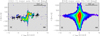 |
Fig. 3. Left panel: observed CO(2−1) p-v diagram along the kinematic major axis (fluxes above 3σ). The black circles correspond to the velocities of the [O III] narrow components along the kinematic major axis. Right panel: same as in the left panel, but for the [O III] emission. The horizontal dashed line indicates the zero velocity, and the vertical line shows the AGN position. |
The left panel of Fig. 4 shows the p-v diagram along the kinematic minor-axis for the molecular gas, which reveals noncircular motions. Leaving aside the nuclear region (inner ∼1″), which was discussed in detail by Alonso-Herrero et al. (2018), the CO(2−1) non-circular motions are observed both to the northeast and southwest of the AGN extending for several arcseconds. The typical amplitudes of the noncircular motions are ∼50 km s−1 and are blueshifted and redshifthed on either side of the AGN. This indicates that outflowing and inflowing motions are present out to distances of ∼6″ (500 pc) from the AGN. To interpret the CO(2−1) noncircular motions, we first discarded density wave-driven inflows. We took into account the orientation of the stellar bar (PA = 85°) and the orientation of the galaxy (see Fig. 2). Assuming that the molecular gas in the disk of the galaxy rotates counter clockwise, the bar-induced streaming motions (local inflow) would be redshifted to the southwest and blueshifted to the northeast along the kinematic minor axis (see Fig. 4, left panel). However, an extraplanar outflow component is not expected because generally, the noncircular velocity is lower than the escape velocity (∼200 km s−1 at 5″), and any extraplanar component would fall back onto the disk. For the molecular gas outflowing motions we therefore make the reasonable assumption that they take place on the plane of the galaxy. Taking into account the geometry model derived by Fischer et al. (2013) for the ionized gas outflow (see Fig. 5) to the east (far side of the disk), the redshifted velocities should trace the molecular outflow, whereas to the west (near side of the disk), we expect blueshifted velocity excess.
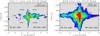 |
Fig. 4. Left panel: observed CO(2−1) p-v diagram along the kinematic minor axis (fluxes above 3σ). Right panel: same as in the left panel, but for the [O III] emission. The black box in the right panel shows the FoV of the left panel. The horizontal dashed lines indicate the zero velocity, and the vertical lines show the AGN position. |
The [O III] p-v diagram along the kinematic major and minor axis is more complex because of the larger number of kinematic components (see the right panels of Figs. 3 and 4). A visual inspection shows that the maximum observed outflow velocities reach ∼1500 km s−1. The high-velocity gas region (∼1000−1500 km s−1) is indeed spatially resolved. The emission appears blueshifted and redshifted at either side of the galaxy. This confirms the 3D nature of the ionized emission of the AGN-driven outflow, which was first inferred by Fischer et al. (2013) with long-slit spectroscopy. The western components are clearly weaker because of the higher extinction derived from the Hα/Hβ ratio at this side of the galaxy (see, e.g., Fig. A.1 of Mingozzi et al. 2019).
4.2.2. Spatially resolved kinematics
As discussed in the previous sections, the majority of the selected regions show two or more different velocity components in each of the gas phases studied here (i.e., molecular and ionized). One component is associated with the host galaxy rotating disk and the others with noncircular movements. To derive the spatially resolved kinematics of the in- and outflows in this galaxy, we subtracted the galaxy rotation from the ionized and molecular gas velocity profiles. After we identified the rotation disk components, we subtracted the corresponding velocity of the galaxy disk component in each selected region from the other noncircular velocity components.
The median value (projected) for the central velocity of the molecular phase noncircular motions is 44 ± 29 km s−1 with most regions show velocities below 100 km s−1. The only exceptions are three eastern regions corresponding to CO(2−1) clumps located at projected distances of ∼10−16″ (∼0.9−1.3 kpc) and one in the western region at ∼10″ (∼0.8 kpc). The ionized gas outflow normally shows higher velocities, reaching central velocities of ∼720 km s−1 (projected) in regions close to the AGN.
Figure 6 shows the spatial distribution of Vcentral (projected) of the [O III] outflowing kinematic components, both blueshifted (top) and redshifted (bottom). According to the ionization cone modelling of Fischer et al. (2013), the ionization cone has an inclination angle of ∼40° with respect to the host galaxy disk (see Fig. 5) and an opening angle of ∼110°. Based on this, blueshifted velocities are expected at either side of the galaxy for the ionized phase, as first noted in the minor-axis [O III] p-v diagram. The outflow zone is mainly dominated by blueshifted [O III] velocities (Fig. 6, top). However, redshifted [O III] velocities are also detected in the northeastern and southwestern borders of the outflow, and in the central-eastern part of the outflow (Fig. 6, bottom). This might be explained by a hollow ionization cone (Fischer et al. 2013) and would mean that we are observing the internal wall of the hollow ionization cone in the northeastern part. In the case of the southwestern border and the central-eastern region of the outflow, the material is likely outflowing behind the galaxy disk. These findings together with the geometry derived by Fischer et al. (2013) suggest that the outflow wind and the radio jet should be impacting the galaxy disk.
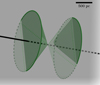 |
Fig. 5. 3D scheme for the geometry of NGC 5643 derived from the NLR modeling by Fischer et al. (2013). The green bicone indicates the AGN outflow, and its axis is illustrated as a black line. The gray plane corresponds to the disk of the host galaxy. Shaded dark and light green regions are in front of and behind the galaxy disk, respectively. North is up and east is left. |
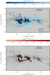 |
Fig. 6. [O III]λ5007 Å integrated intensity map in gray scale. Blue and brown contours show the [O III]λ5007 Å and Hα emission (see Sect. 4). The square regions are color-coded according to the central (projected) outflow velocity in the ionized gas phase. Top panel: blueshifted [O III] outflow vcentral (projected), and bottom panel: redshifted velocities. The solid and dashed green lines correspond to the direction of the radio jet. The dashed orange lines trace the three main absorption features in the dust structure map of Davies et al. (2014). The feature to the southwest may be associated with outflow rather than inflow. |
Figure 7 shows the spatial distribution for the noncircular motions of the CO(2−1) emission. As we showed in the minor-axis p-v diagram (Fig. 4), some are associated with streaming motions linked to the gas response of the bar along the leading edges of the spiral arms. We therefore interpret the CO(2−1) blueshifted (reshifted) noncircular motions in the northern (southern) part of the spiral arms as local inflow. We marked these regions with green crosses for reference. Indeed, CO(2−1) streaming motions like this that are associated with bars are detected in other Seyfert galaxies (e.g., Alonso-Herrero et al. 2019; Shimizu et al. 2019; Domínguez-Fernández et al. 2020). The CO(2−1) noncircular motions in the remaining regions in the east-west [OIII] outflow region can therefore be explained as molecular gas entrained by the AGN wind and outflowing in the plane of the galaxy (see also Alonso-Herrero et al. 2018). We finally note that the velocities of the outflowing and inflowing molecular gas are similar (see also Domínguez-Fernández et al. 2020), and detailed studies such as the one presented here, with a good understanding of the geometry of galaxy and presence of a bar, are therefore required to be able to distinguish them.
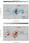 |
Fig. 7. ALMA CO(2−1) integrated intensity map in gray scale. Blue contours show the [O III]λ5007 Å emission (see Sect. 4). The black contours are the CO(2−1) emission on a logarithmic scale with the first contour at 6σ and the last contour at 2.2 × 10⁻¹⁷ erg s−1 cm2 beam−1. The square regions are color-coded according to the central (projected) noncircular velocity in the cold molecular gas phase. Top panel: blueshifted CO(2−1) noncircular Vcentral (projected), and bottom panel: redshifted velocities. The solid black line shows the orientation of the large-scale stellar bar (Mulchaey et al. 1997). Filled green stars mark regions with the expected local inflow regions due to the bar (see Sect. 4.2). The dashed orange lines are the same as in Fig. 6. |
5. Multiphase outflow connection
5.1. Spatially resolved outflow properties
The relation between the various phases of AGN-driven outflows has previously been studied in active galaxies from the integrated approach and generally not for the same galaxies (e.g., Fiore et al. 2017). In this section we examine the spatially resolved properties of the outflow of NGC 5643 in the molecular and ionized phases. Figure 8 shows the spatial profile of the outflowing Vcentral (projected) for the ionized phase (right panel) and the central outflowing velocities (projected) for the molecular gas (left panel) phase along the east-west direction. The ionized outflow shows the highest outflow velocities relatively close (projected distances of approximately 400 pc) to the AGN, with the Vcentral (projected) reaching ∼720 km s−1 blueshifted to the east of the AGN and redshifted to the west. On the eastern side of the galaxy, the outflowing ionized gas is decelerated rapidly from ∼720 km s−1 to 100−200 km s−1 (projected velocities) at 5−6″ (projected distances of ∼400−500 pc). The electron density map (see, e.g., Fig. B.1 of Mingozzi et al. 2019) reveals higher values of the electron density in this region, which might be related with the compression effect of the outflow-induced shocks (e.g., Villar et al. 2014, 2015; Arribas et al. 2014). This region also coincides with the region that is depleted of molecular gas that was first noted in the integrated CO(2−1) map. This suggests that in this region, the AGN-driven wind impacted the host galaxy. See Sect. 5.3 for further discussion.
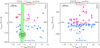 |
Fig. 8. Spatially resolved profile of the central outflow velocities (projected) for CO(2−1) (left) and for [O III] (right). Blue and red symbols correspond to blueshifted and redshifted velocities. For comparison, we also show the central velocities of the slices (pale blue and magenta squares; see Sects. 3.2 and 4, and Appendix A). The black circle indicates the cleared molecular gas region. |
Because the signatures of the gas outflow are relatively weak in the individual regions, we used the slices analyzed in Sects. 3.2 and 4 to derive the outflow properties (see also Appendix A). We assumed that the molecular outflow occurs in the galaxy disk, therefore we can calculate their deprojected noncircular velocities as

where i is the inclination angle of the galaxy disk and Ψ is the phase angle measured in the galaxy plane from the receding side of the line of nodes. The median deprojected outflowing velocity of the cold molecular gas is ∼189 km s−1.
As previously discussed, the nature of the ionized phase of NGC 5643 is 3D with a hollow ionization cone. Therefore we used the outflow geometry of NGC 5643 derived from the NLR modelling by Fischer et al. (2013) to correct the ionized outflow velocities. We deprojected the central velocities of the ionized outflow taking the inclination angles of each wall of the cone into account. Following Fischer et al. (2013), the inclination angle of the bicone with respect to the plane of the sky is 25° and the hollow ionization bicone has internal and external semiopening angles of 50° and 55°, respectively. Therefore the correction factor is more important for redshifted (blueshifted) velocities at the eastern (western) side of the cone (angle of 27.5°). However, the applied correction factor for the blueshifted (redshifted) velocities at the eastern (western) side of the cone is small (angle of 77.5°). The deprojected outflowing velocities of the ionized gas reach velocities (blueshifted and redshifted) of up to ∼750 km s−1 at either side of the galaxy.
To calculate the mass outflow rate of the ionized phase in each slice, we used the extinction-corrected [O III] luminosities of the outflowing component and derived electron densities using the same method as in Fiore et al. (2017),
![$$ \begin{aligned} M_{\rm out}^\mathrm{[O\,III]} = 4.0\times 10^{7}\,M_\odot \left(\frac{C}{10^\mathrm{O/H}} \right)\left(\frac{{L}_{\mathrm{[O\,III]\,out}}}{10^{44}\,\mathrm{erg\,s^{-1}}} \right)\left(\frac{n_{\rm e}}{1000\,\mathrm{cm^{-3}}} \right)^{-1} , \end{aligned} $$](/articles/aa/full_html/2021/01/aa38256-20/aa38256-20-eq11.gif)
where L[O III] out is the [O III] emission line luminosity in units of 1044 erg s−1, ne is the electron density in the ionized gas clouds in units of 103 cm−3 (see Table A.1), 10[O/H] is the oxygen abundance in solar units ([O/H]⊙ ∼ 8.86; Centeno & Socas-Navarro 2008) and C is the condensation factor. This last parameter can be approximated as C = 1 under the assumption that all ionizing gas clouds have the same density (see, e.g., Cano-Díaz et al. 2012 for further details). For the oxygen abundance we used the median value of [O/H] = 9.0 derived for the NLR of NGC 5643 (Storchi-Bergmann et al. 1998). This estimate also assumes a fully ionized gas with an electron temperature of 104 K. We finally assumed that the total ionized gas mass is 3 × M[O III] (see Fiore et al. 2017). The largest source of uncertainty in this measure is related to the electron density (see, e.g., Harrison et al. 2018).
For the outflowing molecular gas mass we used the CO(2−1) fluxes. Because the CO-to-H2 conversion factor is poorly constrained for Seyfert galaxies, we took the Galactic conversion factor (αCO = Mgas/ = 4.35 M⊙[K km s−1 pc2]−1; Bolatto et al. 2013) and a the CO(1−0)/CO(2−1) brightness temperature ratio of one. The molecular gas mass depends on the assumed conversion factor, αCO, and on the CO(1−0)/CO(2−1) ratio. Some previous works also used the conversion factor of ultraluminous infrared galaxies (ULIRGs) (αCO = 0.8 M⊙[K km s−1 pc2]−1; Bolatto et al. 2013; Cicone et al. 2014; Lutz et al. 2020), therefore we discuss the results using
  and
and  conversion factors. The latter would reduce our estimate by a factor of ∼5, and, therefore the results do not change significantly (see Appendix D). We used the method developted by Solomon & Vanden Bout (2005) to estimate the molecular gas mass that includes a correction factor (36%) to include the He mass. The assumed uncertainty of the molecular gas mass using the Galactic conversion factor is ∼30% (e.g., Bolatto et al. 2013).
The mass outflow rate for both molecular and ionized phases can be calculated as
where Mout is the outflowing mass, vout is the outflowing velocity, and ΔD is the size of our slices (2.4″ ∼ 192 pc). The outflow kinetic power and momentum are

Figure 9 shows the spatially resolved properties of the outflow at either side of the AGN for the ionized and molecular phases. The spatial profiles of the outflowing mass for both phases are clearly different. The maximum outflowing mass at the eastern side for the ionized phase coincides with the minimum (or lack) of outflowing molecular gas at the eastern side of the AGN. However, the outflowing gas masses are higher for the molecular phase than for the ionized phase. The ratio is ∼600 (110 for a ULIRG αCO), which is higher than the uncertainties. Similarly, the molecular gas mass outflow rate profile has higher values than the profile the ionized phase (see the top right panel of Fig. 9), but in this case, the ratio between the ionized and molecular phase is lower ∼360 (70 for a ULIRG αCO).
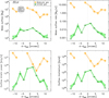 |
Fig. 9. Spatially resolved properties of the ionized (green circles) and molecular (orange squares) phases of the outflow: outflowing mass (top left), mass outflow rate (top right), outflow kinetic power (bottom left), and outflow momentum (bottom right). Orange squares and green circles correspond to the molecular and ionized outflow gas, respectively. The two regions to the east of the AGN (negative d − dAGN values) with no molecular outflow derived properties correspond to regions with cleared CO(2−1) emission. |
The profiles of the outflow kinetic power and momentum (see central panels of Fig. 9) of both phases decrease at ∼5−10″ (∼400−800 pc). However, the kinetic power and momentum profiles in the ionized phase show a local minimum in the eastern side at ∼5″ (∼400 pc) where the AGN wind is probably impacting the galaxy strongly. We find tentative evidence of clearing of the molecular gas as a result of the interaction of the AGN wind with molecular gas in the galaxy (see Sect. 5.3), including that the outflowing component coincides with the location where the AGN wind is decelerated. The profile of the eastern part shows a lack of outflowing molecular mass in the cleared gas region. Interestingly, at this side of the outflow, the farthest slice regions show higher values of the outflowing molecular mass content, which is comparable to the slices in the inner region. This agrees with the clearing and pushing-gas scenario proposed here.
5.2. Integrated outflow properties
Table 1 reports the main integrated outflow properties on either side of the nucleus. The molecular gas outflowing mass of the eastern side, Mout, molecular ∼ 3.5 × 10⁷ M⊙ (0.6 × 10⁷ M⊙ for a ULIRG αCO), is roughly twice that of the western side. However, in the ionized phase, the outflowing mass in the eastern region (Mout, ionized ∼ 5.1 × 10⁴ M⊙) is comparable to that at the western side (see the top left panel of Fig. 9). In Appendix C we also present the results for the observed values (i.e., without the extinction correction).
Summary of the molecular and ionized outflow properties.
The molecular gas outflow kinetic power and momentum are ∼80 and ∼170 (∼15 and ∼30 for a ULIRG αCO) times higher than the values of the ionized phase. Moreover, the eastern part of the galaxy appears to be more affected by the AGN-driven outflow based on the lack of molecular gas at this side of the galaxy (see Sects. 4.1 and 5.1). Interestingly, Cresci et al. (2015) also found evidence of positive AGN feedback in the star-forming clumps at ∼6−8″ (∼500−650 pc) in this part of the galaxy. All this suggests that outflows in Seyfert galaxies such as that studied here for NGC 5643 can produce both positive and negative (mild) feedback processes.
Finally, in Fig. 10 we compare the total derived properties for NGC 5643 and the properties for other AGN (e.g., Fiore et al. 2017; Baron & Netzer 2019). For the AGN luminosity of NGC 5643 (Lbol = 8.14 × 1043 erg s−1; Ricci et al. 2017)4, the derived outflow mass and kinematic rates for both gas phases are compatible with the values derived for other AGN. The total momentum rates for the molecular and ionized gas are Ṗout ∼ 7.2 × 1034 (∼1.3 × 1034 for a ULIRG αCO) and ∼4.2 × 1032 dyne, respectively. These values are similar to the radiation momentum rate expected for the AGN in NGC 5643 (ṖAGN = Lbol/c = 2.72 × 1033 dyne). Therefore the wind momentum loads (Ṗout/ṖAGN) for the molecular and ionized outflow phases are ∼27 (∼5 for a ULIRG αCO) and < 1, which is consistent with the derived values of other AGN of similar luminosity (Fiore et al. 2017). This indicates that the outflow molecular phase is not momentum conserving, while the ionized phase most certainly is (Ṗout/ṖAGN < 1). This increase in molecular phase momentum implies that part of the kinetic energy from the AGN wind is transmitted to the molecular outflow. These results suggest that radiative and kinetic AGN feedback modes coexist in NGC 5643.
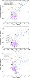 |
Fig. 10. Total outflow properties. Top panel: outflow mass rate as a function of the AGN luminosity. The dashed orange and solid green lines are the best-fit correlations derived by Fiore et al. (2017) for the molecular and ionized gas, respectively. Middle panel: same as top panel, but for the outflow kinetic power. Solid, dashed, dotted, and dash-dotted lines represent Ėkin = 1.0,0.1,0.01,0.001 Lbol. Bottom panel: kinetic coupling efficiencies. The various horizontal lines correspond to theoretical values (Costa et al. 2018; Di Matteo et al. 2005; Dubois et al. 2014; Hopkins & Elvis 2010; Schaye et al. 2015; Weinberger et al. 2017). Orange stars and green squares represent the values derived in this work for the molecular and ionized phase of NGC 5643, respectively. The black circle shows the total kinetic coupling efficiencies for both (ionzed and molecular) gas phases. The brown hourglass and blue circles are taken from Fiore et al. (2017) for the molecular and ionized phase, respectively, and the purple triangles are adopted from Baron & Netzer (2019) for ionized outflows. We have consistently applied the same method as in Fiore et al. (2017) for the total ionized gas mass, as |
![$ 3\times M_{\mathrm{out}}^{\mathrm{[O\,III]}} $](/articles/aa/full_html/2021/01/aa38256-20/aa38256-20-eq28.gif)
In addition, the presence of a radio jet in NGC 5643 might play a role in injecting outflow power. Following the method presented in Bîrzan et al. (2008) using the monochromatic luminosity at 1.4 GHz of the NGC 5643 jet (Meléndez et al. 2010), we find that the jet power is ∼2−10 ×  and ∼160 ×
  . This indicates that the jet of NGC 5643 can contribute to driving the molecular and ionized outflows efficiently.
On the other hand, the bottom panel of Fig. 10 shows the kinetic coupling efficiencies for molecular and ionized outflows. Although the various assumptions and methods employed in the literature might be responsible for some of the scatter, the range of values for a fixed AGN bolometric luminosity in this plot is wide (about eight orders of magnitude). It is of interest to compare the observed kinetic powers from those derived from AGN feedback models (see, e.g., Harrison et al. 2018). The values derived in this work (see also Appendix D) for the molecular and ionized outflow of NGC 5643 agree well with the theoretical values reported by Hopkins & Elvis (2010) and Costa et al. (2018).
5.3. Destruction or clearing of the molecular gas
As previously discussed in Alonso-Herrero et al. (2018), see also Sect. 4.1, there is a deficit of CO(2−1) emission at the eastern side of the spiral. This might be related to the destruction or clearing of the molecular gas produced by the AGN wind impacting on the host galaxy. To estimate the possible impact of the outflow wind on the destruction or clearing of the molecular gas, we therefore measured the total gas mass in both spiral arms. To do so, using the fully reduced optical HST/F606W image of NGC 5643 from the ESA Hubble Legacy Archive5, we defined the region of the two main spiral arms. Then, using the CO(2−1) data, we extracted several regions following both spiral arms (see Fig. B.1). See Appendix B for further details on the selection of the spiral arm regions.
Figure 11 shows the cumulative molecular gas mass profile, which confirms the molecular gas deficit in the eastern part of the galaxy reveals by the CO(2−1) emission map. The molecular gas mass of the eastern spiral arm using two different approaches (see Appendix B) is Meast ∼ (1.5−2.0) × 107 M⊙ ( ). This is only 50−70% of the molecular gas content in the western spiral arms. This should be related to the destruction or clearing of the molecular gas produced by the AGN wind strongly impacting on the eastern side of the host galaxy. The molecular gas content in the spiral arms is comparable to the outflowing molecular mass in the outflow regions. However, note that for the spiral arms we did not include regions in the nuclear regions, which accounts for the bulk of the molecular gas mass in the disk and in the molecular outflow. We also note that we calculated the deficit of molecular gas in the eastern part of the galaxy under the assumption of symmetry in the surface brightness. However, it is possible that intrinsic variations in the surface brightness due to asymmetry might affect this measurement.
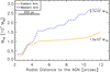 |
Fig. 11. Cumulative molecular mass profiles using the symmetric selected regions in the spiral arms at either side of the nucleus (see Appendix B). Eastern and western sides are shown as solid orange and dashed blue lines, respectively. |
6. Analytic model of the outflow wind
NGC 5643 is an intermediate luminosity AGN with a large outflow extending ∼1 kpc at either side of the nucleus. Previous works studied how the radial extent of the NLR scales with AGN luminosity. The expected radial extent of the ionized phase depends on the relation employed. When we compare the [O III] luminosity of NGC 5643 (log(L[O III]) = 40.4 erg s−1; Meléndez et al. 2008) with Fig. 10 of Fischer et al. (2018), the expected radial extent ranges from ∼100−500 pc. However, this value is much higher (ranging from 0.5−2.5 kpc) for the relation with the 8 μm luminosity6 presented in Fig. 3 of Hainline et al. (2014). Because the observed outflow properties are not well constrained, it is of interest to compare them (e.g., size and velocity) with those estimated from a theoretical point of view. To do so, we followed the analytic model proposed by Das et al. (2007), which considers the radiation-driven wind and the gravitational drag as
where Lbol is the bolometric luminosity of the AGN, σT is the Thomson-scattering cross section for the electron, ξ is the force multiplier, r is the distance, c is the speed of light, mp is the mass of the proton, G is the universal gravitational constant, and M(r) is the total enclosed mass within r. The force multiplier (ξ) is primarily a function of the ionization parameter (U) for a given spectral energy distribution (see Das et al. 2007 and references therein for further discussion). Das et al. (2007) found values of the force multiplier that ranged from ξ ∼ 500−6000 for the Sy2 galaxy NGC 1068 based on photoionization models. This approach takes the drag forces from gravity stopping and turning the gas outflow back into account, but not the possible deceleration of the NLR outflow that results from the resistance of the interstellar medium (ISM).
Using a bulge mass of Mbulge = 5.48 × 10⁹ M⊙, an effective radius of 0.46 kpc (Weinzirl et al. 2009), and a black hole mass MBH = 2.75 × 10⁶ M⊙ (Goulding et al. 2010, and following Eqs. (5)–(7) of Das et al. 2007, we find that the enclosed mass as a function of the distance from the central SMBH) is
Then, integrating Eq. (6) and setting the initial velocity to zero, we obtain the following velocity of the model:
![$$ \begin{aligned} { v}(r) = \sqrt{\int _{r1}^{r} \left[6840 \frac{L_{\rm bol}}{10^{44}} \frac{\xi }{t^2} - 8.6 \times 10^{-3} \frac{M_{\rm tot}(t)}{t^2} \right] \mathrm{d}t}. \end{aligned} $$](/articles/aa/full_html/2021/01/aa38256-20/aa38256-20-eq34.gif)
This model assumed spherical symmetry for the sake of simplicity. We used the same value of the bolometric luminosity as in Sect. 5.2.
In Fig. 12 we show the resulting velocity profiles of NGC 5643 for various launch radii (r1 = 1, 2, 4, 8, 16, 32, and 64 pc) and force multiplier values (ξ = 200, 300, and 400), which reproduce the ionized phase observations well (see the black circles in Fig. 12). Although we did not consider here other drag forces such as the ISM, the value of the force multiplier needed to fit the observational data is quite low compared with the maximum value derived for NGC 1068. This means that even when other drag forces are included, it is possible to reproduce the observations by increasing the force multiplier.
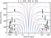 |
Fig. 12. Outflow wind analytic model: velocity profiles for various force multipliers (ξ = 200, 300, and 400) and launch radii (r1 = 1, 2, 4, 8, 16, 32, and 64 pc). Lines correspond to the various force multipliers used (ξ = 200 solid blue, 300 dotted green, and 400 dashed red). Black circles correspond to the deprojected velocities of the ionized outflow. Negative (positive) distances indicate eastern (western) radial distances to the AGN. |
Figure 12 shows that up to a launch radius of r1 = 4 pc, the velocity of the gas quickly reaches terminal velocity, even for the smaller force multiplier (i.e., ξ = 200). This means that it does not slow down significantly with the radii for small launch distances. However, at larger launch radii, the gas velocity starts to turn over and returns to the systemic velocities at r ∼ 100 pc for the smaller force multiplier. These results suggest that in Seyfert galaxies with intermediate AGN luminosities, bulge and BH masses similar to those of NGC 5643, the ionized outflow can reach kiloparsec scales, as observed in this galaxy.
7. Conclusions
We presented a detailed study of the multiphase feedback processes in the central ∼3 kpc of the barred Seyfert 2 galaxy NGC 5643. We used observations of the cold molecular gas (ALMA CO(2−1) transition) and ionized gas (MUSE IFU optical emission lines). We studied different regions along the outflow zone, which extends out to ∼2.3 kpc in the same direction (east-west) as the radio jet, as well as nuclear and circumnuclear regions in the host galaxy disk. The main results are listed below.
-
The [O III]λ5007 Å emission lines in regions in the outflow have two or more components. The narrow component traces the rotation of the gas in the disk. The others, which have broader profiles (median
![$ \sigma_{\mathrm{broad}}^{\mathrm{[O\,III]}} $](/articles/aa/full_html/2021/01/aa38256-20/aa38256-20-eq35.gif) = 233 ± 75 km s−1), are related to the ionized gas outflow. The projected ionized outflow velocities in this phase reach ∼720 km s−1 in the inner 830 pc (∼10″), and are then decelerated at greater distances from the AGN.
= 233 ± 75 km s−1), are related to the ionized gas outflow. The projected ionized outflow velocities in this phase reach ∼720 km s−1 in the inner 830 pc (∼10″), and are then decelerated at greater distances from the AGN. -
The CO(2−1) line profiles of regions in the outflow and in the nuclear and circumnuclear spiral also show two or more different velocity components. One is associated with the rotating disk of the host galaxy, and the others with inflowing and outflowing motions. The streaming motions (local inflow) are due to a large-scale stellar bar.
-
The deprojected outflowing velocities of the cold molecular gas (median Vcentral ∼ 189 km s−1) are generally lower than those of the outflowing ionized gas, which reaches deprojected velocities of up to 750 km s−1 (both blueshifted and redshifted) close to the AGN, and their spatial profiles follow those of the ionized phase, although the velocity profile of the molecular phase follows that of the ionized phase. This suggests that molecular gas in the host galaxy disk is being entrained by the AGN wind in these regions.
-
The molecular and ionized outflow masses are ∼5.2 × 10⁷ M⊙ (∼1.0 × 10⁷ M⊙ for a ULIRG αCO) and 8.5 × 10⁴ M⊙, respectively. Furthermore, the derived molecular and ionized outflow mass rates are ∼51 (9) M⊙ yr−1 and 0.14 M⊙ yr−1. This shows that the molecular phase dominates the outflow mass and outflow mass rate: the ratios are higher by 600 (110) and 360 (70) than those of the ionized phase.
-
The outflow kinematic power for both outflow gas phases is similar. Interestingly, the kinematic power shows a strong decrease at projected distances ∼400 pc east and west of the AGN, probably where the greatest effect of the AGN wind impacting the host galaxy is taking place. The wind momentum loads (Ṗout/ṖAGN) for the molecular and ionized outflow phases are ∼27 (5) and < 1, which suggests that the molecular phase is not momentum conserving, while the ionized phase most certainly is.
-
We estimated the molecular gas mass in the two main spiral arms in the circumnuclear region of NGC 5643. The molecular gas mass of the eastern spiral arm, Meast ∼ 1.5 × 10⁷ M⊙, is 50−70% of the content of the western arm. This should be related, at least in part, with the destruction or clearing of the molecular gas produced by the AGN wind impacting on the eastern side of the host galaxy.
-
Using a simple analytic model of a radiation-driven AGN wind and gravitational drag, we reproduced the ∼2 kpc scale outflow observed in NGC 5643. This suggests that for AGN luminosities, bulge, and BH masses such as in this galaxy, ionized outflows can reach large scales.
All of these results suggest that outflows in Seyfert-like AGN such as in NGC 5643 can produce both positive (Cresci et al. 2015) and negative (mild) feedback processes. In particular, in the Seyfert galaxy NGC 5643, the molecular phase does not conserve momentum, while the ionized phase most certainly does. This suggests that radiative or quasar and kinetic or radio AGN feedback modes coexist and may shape the host galaxies even at kiloparsec scales. Although there have been only a few detailed multiphase studies using various regions within the same source to date, it is essential to quantify the overall outflow properties of each phase. Future observations of large samples, combining high-resolution optical and submillimeter observations, will be able to characterize the typical effect of AGN feedback on the host galaxy.
We calculated the bolometric luminosity using the intrinsic 14−195 keV Swift/BAT luminosity from Ricci et al. (2017) and a fixed bolometric correction (Lbol/L14−195 keV = 7.42; García-Bernete et al. 2019).
The 8 μm luminosity (log(L8 μm) = 42.2 erg s−1) was calculated by taking the average of a 1 μm window centred at 8 μm in the Spitzer spectrum (see Sect. 2.3).
The optical integral field spectroscopy of NGC 7009 was taken using VLT/MUSE, which was observed as part of the program 60.A-9347. We downloaded the fully reduced and calibrated science data cube from the ESO data archive. This MUSE data cube, previously presented in Walsh et al. (2018), was observed under similar seeing conditions (∼0.5 ″) as the one used in this work for NGC 5643.
Acknowledgments
IGB, AAH, and FJC acknowledge financial support through grant PN AYA2015-64346-C2-1-P (MINECO/FEDER), funded by the Agencia Estatal de Investigación, Unidad de Excelencia María de Maeztu. IGB and DR also acknowledge support from STFC through grant ST/S000488/1. DR acknowledges support from the University of Oxford John Fell Fund. AAH, SGB and MVM also acknowledge support through grant PGC2018-094671-B-I00 (MCIU/AEI/FEDER,UE). AAH, MPS, MVM and AL work was done under project No. MDM-2017-0737 Unidad de Excelencia “María de Maeztu” – Centro de Astrobiología (INTA-CSIC). MPS acknowledges support from the Comunidad de Madrid, Spain, through Atracción de Talento Investigador Grant 2018-T1/TIC-11035 and PID2019-105423GA-I00 (MCIU/AEI/FEDER,UE). BG-L acknowledges support from the State Research Agency (AEI) of the Spanish Ministry of Science, Innovation and Universities (MCIU) and the European Regional Development Fund (FEDER) under grant with reference AYA2015-68217-P. FJC and SM acknowledge financial support from the Spanish Ministry MCIU under project RTI2018-096686-B-C21 (MCIU/AEI/FEDER/UE), cofunded by FEDER funds and from the Agencia Estatal de Investigación, Unidad de Excelencia María de Maeztu, ref. MDM-2017-0765. CRA acknowledges support from the Spanish Ministry of Science, Innovation and Universities (MCIU), the Agencia Estatal de Investigación (AEI) and the Fondo Europeo de Desarrollo Regional (EU FEDER) under project AYA2016-76682-C3-2-P and PID2019-106027GB-C42. CRA also acknowledges support from the MCIU under grant RYC-2014-15779. AL acknowledges the support from Comunidad de Madrid through the Atracción de Talento grant 2017-T1/TIC-5213. CR acknowledges support from the Fondecyt Iniciacion grant 11190831. This paper makes use of the following ALMA data: ADS/JAO.ALMA#2016.1.00254.S. This work is based [in part] on archival data obtained with the Multi Unit Spectroscopic Explorer (MUSE) on the Very Large Telescope (VLT) under ESO programme 095.B-0532(A), and the Spitzer Space Telescope, which is operated by the Jet Propulsion Laboratory, California Institute of Technology under a contract with NASA. This research has also made use of the NASA/IPAC Extragalactic Database (NED), which is operated by the Jet Propulsion Laboratory, California Institute of Technology under a contract with NASA. Finally, we are extremely grateful to the anonymous referee for useful comments.
References
- Alonso-Herrero, A., Pereira-Santaella, M., García-Burillo, S., et al. 2018, ApJ, 859, A144 [NASA ADS] [CrossRef] [Google Scholar]
- Alonso-Herrero, A., García-Burillo, S., Pereira-Santaella, M., et al. 2019, A&A, 628, A65 [NASA ADS] [CrossRef] [EDP Sciences] [Google Scholar]
- Arribas, S., Colina, L., Bellocchi, E., Maiolino, R., & Villar-Martín, M. 2014, A&A, 568, A14 [NASA ADS] [CrossRef] [EDP Sciences] [Google Scholar]
- Bacon, R., Accardo, M., Adjali, L., et al. 2010, Proc. SPIE, 7735, 773508 [Google Scholar]
- Baron, D., & Netzer, H. 2019, MNRAS, 482, 3915 [NASA ADS] [CrossRef] [Google Scholar]
- Bennert, N., Jungwiert, B., Komossa, S., Haas, M., & Chini, R. 2006a, A&A, 456, 953 [NASA ADS] [CrossRef] [EDP Sciences] [Google Scholar]
- Bennert, N., Jungwiert, B., Komossa, S., Haas, M., & Chini, R. 2006b, A&A, 459, 55 [NASA ADS] [CrossRef] [EDP Sciences] [Google Scholar]
- Bîrzan, L., McNamara, B. R., Nulsen, P. E. J., Carilli, C. L., & Wise, M. W. 2008, ApJ, 686, 859 [NASA ADS] [CrossRef] [Google Scholar]
- Bolatto, A. D., Wolfire, M., & Leroy, A. K. 2013, ARA&A, 51, 207 [Google Scholar]
- Bongiorno, A., Schultze, A., Merloni, A., et al. 2016, A&A, 588, A78 [NASA ADS] [CrossRef] [EDP Sciences] [Google Scholar]
- Bower, R. G., Benson, A. J., Malbon, R., et al. 2006, MNRAS, 370, 645 [NASA ADS] [CrossRef] [Google Scholar]
- Bruzual, G., & Charlot, S. 2003, MNRAS, 344, 1000 [NASA ADS] [CrossRef] [Google Scholar]
- Calzetti, D., Armus, L., Bohlin, R. C., et al. 2000, ApJ, 533, 682 [NASA ADS] [CrossRef] [Google Scholar]
- Cano-Díaz, M., Maiolino, R., Marconi, A., et al. 2012, A&A, 537, L8 [NASA ADS] [CrossRef] [EDP Sciences] [Google Scholar]
- Cappellari, M. 2017, MNRAS, 466, 798 [NASA ADS] [CrossRef] [Google Scholar]
- Cappellari, M., & Copin, Y. 2003, MNRAS, 342, 345 [NASA ADS] [CrossRef] [Google Scholar]
- Cappellari, M., & Emsellem, E. 2004, PASP, 116, 138 [NASA ADS] [CrossRef] [Google Scholar]
- Centeno, R., & Socas-Navarro, H. 2008, ApJ, 682, L61 [NASA ADS] [CrossRef] [Google Scholar]
- Cicone, C., Maiolino, R., Sturm, E., et al. 2014, A&A, 562, A21 [NASA ADS] [CrossRef] [EDP Sciences] [Google Scholar]
- Cicone, C., Brusa, M., Ramos, Almeida C., et al. 2018, Nat. Astron., 2, 176 [Google Scholar]
- Cid, Fernandes R., Mateus, A., Sodré, L., Stasińska, G., & Gomes, J. M. 2005, MNRAS, 358, 363 [NASA ADS] [CrossRef] [Google Scholar]
- Costa, T., Rosdahl, J., Sijacki, D., & Haehnelt, M. G. 2018, MNRAS, 473, 4197 [NASA ADS] [CrossRef] [Google Scholar]
- Cresci, G., Marconi, A., Zibetti, S., et al. 2015, A&A, 582, A63 [NASA ADS] [CrossRef] [EDP Sciences] [Google Scholar]
- Croton, D. J., Springel, V., White, S. D. M., et al. 2006, MNRAS, 365, 11 [NASA ADS] [CrossRef] [Google Scholar]
- Das, V., Crenshaw, D. M., & Kraemer, S. B. 2007, ApJ, 656, 699 [NASA ADS] [CrossRef] [Google Scholar]
- Davies, R. I., Maciejewski, W., Hicks, E. K. S., et al. 2014, ApJ, 792, 101 [NASA ADS] [CrossRef] [Google Scholar]
- Davies, R., Baron, D., Shimizu, T., et al. 2020, MNRAS, 498, 4150 [Google Scholar]
- de Vaucouleurs, G., de Vaucouleurs, A., & Corwin, H. G., Jr. 1976, Second Reference Catalogue of Bright Galaxies (Austin: Univ. Texas Press) [Google Scholar]
- Di Matteo, T., Springel, V., & Hernquist, L. 2005, Nature, 433, 604 [NASA ADS] [CrossRef] [PubMed] [Google Scholar]
- Di Teodoro, E. M., & Fraternali, F. 2015, Astrophysics Source Code Library [record ascl:1507.001] [Google Scholar]
- Domínguez-Fernández, A. J., Alonso-Herrero, A., García-Burillo, S., et al. 2020, A&A, 643, A127 [CrossRef] [EDP Sciences] [Google Scholar]
- Dubois, Y., Pichon, C., Welker, C., et al. 2014, MNRAS, 444, 1453 [NASA ADS] [CrossRef] [Google Scholar]
- Erroz-Ferrer, S., Carollo, C. M., den Brok, M., et al. 2019, MNRAS, 484, 5009 [NASA ADS] [CrossRef] [Google Scholar]
- Fiore, F., Feruglio, C., Shankar, F., et al. 2017, A&A, 601, A143 [NASA ADS] [CrossRef] [EDP Sciences] [Google Scholar]
- Fischer, T. C., Crenshaw, D. M., Kraemer, S. B., & Schmitt, H. R. 2013, ApJS, 209, 1 [NASA ADS] [CrossRef] [Google Scholar]
- Fischer, T. C., Kraemer, S. B., Schmitt, H. R., et al. 2018, ApJ, 856, 102 [NASA ADS] [CrossRef] [Google Scholar]
- García-Bernete, I., Ramos Almeida, C., Alonso-Herrero, A., et al. 2019, MNRAS, 486, 920 [Google Scholar]
- García-Burillo, S., Combes, F., Usero, A., et al. 2014, A&A, 567, A125 [NASA ADS] [CrossRef] [EDP Sciences] [Google Scholar]
- García-Burillo, S., Combes, F., Ramos Almeida, C., et al. 2019, A&A, 632, A61 [CrossRef] [EDP Sciences] [Google Scholar]
- Ginsburg, A., & Mirocha, J. 2011, Astrophysics Source Code Library [record ascl:1109.001] [Google Scholar]
- Goulding, A. D., Alexander, D. M., Lehmer, B. D., & Mullaney, J. R. 2010, MNRAS, 406, 597 [NASA ADS] [CrossRef] [Google Scholar]
- Hainline, K. N., Hickox, R. C., Greene, J. E., et al. 2014, ApJ, 787, 65 [NASA ADS] [CrossRef] [Google Scholar]
- Harrison, C. M., Costa, T., Tadhunter, C. N., et al. 2018, Nat. Astron., 2, 198 [NASA ADS] [CrossRef] [Google Scholar]
- Hopkins, P. F., & Elvis, M. 2010, MNRAS, 401, 7 [NASA ADS] [CrossRef] [Google Scholar]
- Houck, J. R., Roellig, T. L., van Cleve, J., et al. 2004, ApJS, 154, 18 [NASA ADS] [CrossRef] [Google Scholar]
- Klamer, I. J., Ekers, R. D., Sadler, E. M., & Hunstead, R. W. 2004, ApJ, 612, L97 [NASA ADS] [CrossRef] [Google Scholar]
- Lebouteiller, V., Barry, D. J., Spoon, H. W. W., et al. 2011, ApJS, 196, 8 [NASA ADS] [CrossRef] [Google Scholar]
- Leipski, C., Falcke, H., Bennert, N., & Hüttemeister, S. 2006, A&A, 455, 161 [NASA ADS] [CrossRef] [EDP Sciences] [Google Scholar]
- Luridiana, V., Morisset, C., & Shaw, R. A. 2015, A&A, 573, A42 [NASA ADS] [CrossRef] [EDP Sciences] [Google Scholar]
- Lutz, D., Sturm, E., Janssen, A., et al. 2020, A&A, 633, A134 [NASA ADS] [CrossRef] [EDP Sciences] [Google Scholar]
- Maiolino, R., Russell, H. R., Fabian, A. C., et al. 2017, Nature, 544, 202 [NASA ADS] [CrossRef] [Google Scholar]
- Meléndez, M., Kraemer, S. B., Armentrout, B. K., et al. 2008, ApJ, 682, 94 [Google Scholar]
- Meléndez, M., Kraemer, S. B., & Schmitt, H. R. 2010, MNRAS, 406, 493 [CrossRef] [Google Scholar]
- Mingozzi, M., Cresci, G., Venturi, G., et al. 2019, A&A, 622, A146 [NASA ADS] [CrossRef] [EDP Sciences] [Google Scholar]
- Morganti, R. 2017, Front. Astron. Space Sci., 4, 42 [NASA ADS] [CrossRef] [Google Scholar]
- Morris, S., Ward, M., Whittle, M., Wilson, A. S., & Taylor, K. 1985, MNRAS, 216, 193 [NASA ADS] [CrossRef] [Google Scholar]
- Mulchaey, J. S., Regan, M. W., & Kundu, A. 1997, ApJS, 110, 299 [NASA ADS] [CrossRef] [Google Scholar]
- Norris, R. P. 2009, ASP Conf. Ser., 408, 380 [Google Scholar]
- Osterbrock, D. E., & Ferland, G. J. 2006, Astrophysics of Gaseous Nebulae and Active Galactic Nuclei (Sausalito, CA: University Science Books) [Google Scholar]
- Ricci, C., Trakhtenbrot, B., Koss, M. J., et al. 2017, ApJS, 233, 17 [NASA ADS] [CrossRef] [Google Scholar]
- Schaye, J., Crain, R. A., Bower, R. G., et al. 2015, MNRAS, 446, 521 [Google Scholar]
- Schmitt, H. R., Storchi-Bergmann, T., & Baldwin, J. A. 1994, ApJ, 423, 237 [NASA ADS] [CrossRef] [Google Scholar]
- Shin, J., Woo, J.-H., Chung, A., et al. 2019, ApJ, 881, 147 [CrossRef] [Google Scholar]
- Shimizu, T. T., Davies, R. I., Lutz, D., et al. 2019, MNRAS, 490, 5860 [NASA ADS] [CrossRef] [Google Scholar]
- Silk, J., & Mamon, G. A. 2012, Res. Astron. Astrophys., 12, 917 [NASA ADS] [CrossRef] [Google Scholar]
- Simpson, C., Wilson, A. S., Bower, G., et al. 1997, ApJ, 474, 121 [NASA ADS] [CrossRef] [Google Scholar]
- Solomon, P. M., & Vanden Bout, P. A. 2005, ARA&A, 43, 677 [NASA ADS] [CrossRef] [Google Scholar]
- Storchi-Bergmann, T., Schmitt, H. R., Calzetti, D., & Kinney, A. L. 1998, AJ, 115, 909 [NASA ADS] [CrossRef] [Google Scholar]
- Vaona, L., Ciroi, S., Di Mille, F., et al. 2012, MNRAS, 427, 1266 [NASA ADS] [CrossRef] [Google Scholar]
- Villar, Martín M., Emonts, B., Humphrey, A., et al. 2014, MNRAS, 440, 3202 [NASA ADS] [CrossRef] [Google Scholar]
- Villar, Martín M., Bellocchi, E., Stern, J., et al. 2015, MNRAS, 454, 439 [NASA ADS] [CrossRef] [Google Scholar]
- Walsh, J. R., Monreal-Ibero, A., Barlow, M. J., et al. 2018, A&A, 620, A169 [NASA ADS] [CrossRef] [EDP Sciences] [Google Scholar]
- Weinberger, R., Springel, V., Hernquist, L., et al. 2017, MNRAS, 465, 3291 [NASA ADS] [CrossRef] [Google Scholar]
- Weinzirl, T., Jogee, S., Khochfar, S., Burkert, A., & Kormendy, J. 2009, ApJ, 696, 411 [NASA ADS] [CrossRef] [Google Scholar]
Appendix A: Stacking regions
To derive the outflow properties, we defined various slices along the outflow at either side of the nucleus. As described in Sect. 3.1, to maximize the S/N of the outflow component, we used the stacking technique. Using the orientation of the large-scale stellar bar (see, e.g., Mulchaey et al. 1997), we divided the selected slices in the outflow into northern and southern regions. Figure A.1 shows the regions where no contribution of from local inflows is expected (black boxes) and those with inflow movements according to bar models (red boxes). In the case of the CO(2−1) line profiles, we indicate the outflow and inflow components (see Figs. A.2 and A.3).
In the case of the [O III] emission profile, it is easy to identify the rotating component of the galaxy disk, which is the narrow component in the line profiles (see Sect. 3.3.2). However, the molecular gas emission is more difficult to distinguish. When possible (high S/N), we used the derived rotating-disk model to identify the rotation component. Otherwise, we selected the brightest line, which we associated with the galaxy disk. The only exceptions are cases that present a large offset (> 100 km s−1) with respect to the immediate previous region. In this situation we searched for continuity in the galaxy disk velocities. We also confirmed that the identified rotation disk component agreed within the errors with the stellar kinematics components derived from the MUSE data (see Sect. 3.3.1). When we identified where the rotation disk components lay, we shifted the velocities to a common rest-frame wavelength.
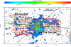 |
Fig. A.1. ALMA CO(2−1) integrated intensity map of NGC 5643 produced from the natural-weight data cube. The map is shown on a linear color scale. Black contours corresponds to the CO(2−1) emission map. They are shown on a logarithmic scale with the first contour at 3σ and the last contour at 2.2 × 10⁻¹⁷ erg s−1 cm2 beam−1. Brown contours correspond to the [O III]λ5007 Å emission map (see Sect. 4). The dashed black line indicates the kinematic major axis. The solid green line corresponds to the direction of the large-scale stellar bar (Mulchaey et al. 1997). Red and black boxes correspond to regions where streaming motions (local inflow) are expected and are not expected, respectively. For instance, region 5ne consists of 2 × 5 black boxes (1.2″ × 1.2″ square apertures), and the eastern 5 full slice corresponds to 5ne+5se. |
Finally, to rule out any possible contribution of the instrumental profile wings at the levels of the measured broad emission lines (i.e., outflow components), we compared the observed emission line profile with the instrumental one. The instrumental profile is defined as the instrument response to an observed unresolved line (i.e., much narrower than the velocity resolution), which depends on the employed instrumentation. This profile can be slightly asymmetric and/or present broad weak wings. To characterize it, we use VLT/MUSE data of the planetary nebula NGC 7009, which is an unresolved source (the velocity extent of the emission line components is ∼60 km s−1; see Walsh et al. 2018) to obtain the [O III] emission line profile in various regions7. The VLT/MUSE spectral resolution is ∼75 km s−1. Because the various regions produce practically the same profile, we used the aperture that was extracted in the center of the nebula. We find that the MUSE/VLT instrumental profile at λ5007 Å is slightly asymmetric, but the detected broad lines in our work cannot be explained by an instrumental effect. This confirms that the Gaussian approach is a good approximation to the instrumental profile, and that it provides reliable flux estimates.
Figures A.2–A.5 show the molecular and ionized emission lines profiles for each slice. We measured the various components following the method presented in Sect. 3. Tables A.1 and A.2 report the ionized and molecular outflow measurements, respectively.
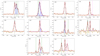 |
Fig. A.2. Molecular CO(2−1) emission-line fitting for the stacked spectra in each slice. Left to right panels: eastern regions 1, 2, 3, 4, and 5. The vertical solid gray line corresponds to the systemic component, the dashed green and dotted pink lines show the components that are identified as outflows and inflows, respectively. The solid orange line corresponds to the fit residuals. |
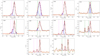 |
Fig. A.3. Molecular CO(2−1) emission-line fitting for the stacked spectra in each slice. Left to right panels: western regions 1, 2, 3, 4, and 5. The vertical solid gray line corresponds to the systemic component, the dashed green and dotted pink lines show the components that are identified as outflows and inflows, respectively. The solid orange line corresponds to the fit residuals. |
Summary of the ionized outflow measurements.
Summary of the molecular nonrotational measurements.
Appendix B: Molecular gas mass of the spiral arms
To estimate the impact of the outflow wind on the destruction of the molecular gas, we measured the total gas mass in both spiral arms. To do so, we first used the fully reduced optical HST/F606W image of NGC 5643 from the ESA Hubble Legacy Archive to define the region of the two main spiral arms. Then, using the ALMA CO(2−1) integrated intensity map, we extracted several regions following both spiral arms (see Fig. B.1). We used two different approaches to measure their CO(2−1): (a) for simplicity, we assumed symmetry in both spiral arms (see the black regions in Fig. B.1); and (b) we complemented this with the remaining CO(2−1) clumps found by visual inspection (see the white regions in Fig. B.1). For both approaches, we find that the molecular gas mass of the eastern spiral arm is Meast ∼ (1.5−2.0) × 107 M⊙. These values correspond to 50−70% to the content of the western arm (see Sect. 5.3).
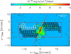 |
Fig. B.1. ALMA CO(2−1) integrated-intensity map of NGC 5643 produced from the natural-weight data cube. The map is shown on a linear color scale. Black contours corresponds to the CO(2−1) emission map. They are shown on a logarithmic scale with the first contour at 8σ and the last contour at 2.2 × 10⁻¹⁷ erg s−1 cm2 beam−1. The various boxes correspond to the regions we selected to measure the two main spiral arms (see Sect. 5.3). Black boxes indicate regions that were selected as symmetric at either side of the nucleus. White boxes correspond to the supplementary regions to take additional individual CO(2−1) clumps into account. The diagonal solid red line indicates the separation axis between the two arms. North is up and east is left, and offsets are measured relative to the AGN. |
Appendix C: Observed outflow properties
In Sect. 5.1 we presented the outflow properties of NGC 5643 using extinction-corrected fluxes. Here we also derived the various outflow properties profiles (see Fig. C.1) without taking the extinction correction into account. As expected, these profiles agree well with the morphology present in the observed [O III] emission map. In Table C.1 we report the main derived observed outflow properties at either side of the nucleus.
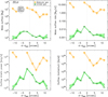 |
Fig. C.1. Observed molecular and ionized gas properties. Top left panel: profile of the mass outflow. Top right panel: profile of the mass outflow rate. Bottom left panel: kinematic power profile of the outflow. Bottom right panel: momentum profile of the outflow. Orange squares and green circles correspond to the molecular and ionized outflow gas phases. The two regions to the east of the AGN (negative d − dAGN values) with no molecular outflow derived properties correspond to regions with cleared CO(2−1) emission. |
Summary of the observed ionized outflow properties.
Appendix D: CO-to-H2 conversion factor
As previously mentioned, the CO-to-H2 conversion factor is poorly constrained for Seyfert galaxies. In Sect. 5.1 we therefore presented the properties of the molecular gas outflow based on the Galactic conversion factor (αCO = Mgas/ = 4.35 M⊙[K km s−1 pc2]−1; Bolatto et al. 2013) and the CO(1−0)/CO(2−1) brightness temperature ratio of one. However, these values depend strongly on the CO-to-H2 conversion factor. Some previous works also used the conversion factor of ULIRGs (see, e.g., Cicone et al. 2014; Lutz et al. 2020). Therefore, for comparison, we also estimated the properties of the molecular gas outflow using a lower CO-to-H2 conversion factor (i.e., the ULIRG factor; αCO = 0.8 M⊙[K km s−1 pc2]−1; Bolatto et al. 2013). Table D.1 and Fig. D.1 show the main properties of the molecular gas outflow at either side of the nucleus using αCO = 0.8 M⊙[K km s−1 pc2]−1. Moreover, Fig. D.2 compares the total derived properties for NGC 5643 and the properties for other AGN, which are discussed in Sect. 5.2. We find that the main results of this work do not change significantly when different CO-to-H2 conversion factors are used.
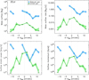 |
Fig. D.1. Spatially resolved properties of the ionized (green circles) and molecular (blue squares) phases of the outflow: outflowing mass (top left), mass outflow rate (top right), outflow kinetic power (bottom left), and outflow momentum (bottom right). Blue squares and green circles correspond to the molecular and ionized outflow gas, respectively. The two regions to the east of the AGN (negative d − dAGN values) with no molecular outflow derived properties correspond to regions with cleared CO(2−1) emission. |
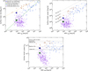 |
Fig. D.2. Total outflow properties. Top left panel: outflow mass rate as a function of the AGN luminosity. The dashed orange and solid green lines are the best-fit correlations derived by Fiore et al. (2017) for the molecular and ionized gas, respectively. Top right panel: same as the top left panel, but for the outflow kinetic power. Solid, dashed, dotted, and dash-dotted lines represent Ėkin = 1.0,0.1,0.01,0.001 Lbol. Bottom panel: kinetic coupling efficiencies. The various horizontal lines correspond to theoretical values (Costa et al. 2018; Di Matteo et al. 2005; Dubois et al. 2014; Hopkins & Elvis 2010; Schaye et al. 2015; Weinberger et al. 2017). Blue stars and green squares represent the values derived in this work for the molecular and ionized phase of NGC 5643, respectively. The black circle shows the total kinetic coupling efficiencies for both (ionzed and molecular) gas phases. Brown hourglass and blue circles are adopted from Fiore et al. (2017) for the molecular and ionized phase, respectively, and the purple triangles are taken from Baron & Netzer (2019) for ionized outflows. We have consistently applied the same method as in Fiore et al. (2017) for the total ionized gas mass, |
![$ 3\times M_{\mathrm{out}}^{\mathrm{[O\,III]}} $](/articles/aa/full_html/2021/01/aa38256-20/aa38256-20-eq48.gif)
Summary of the molecular outflow properties calculated using the ULIRGs CO-to-H2 conversion factor.
All Tables
Summary of the molecular outflow properties calculated using the ULIRGs CO-to-H2 conversion factor.
All Figures
|
Fig. 1. ALMA CO(2−1) integrated intensity map of NGC 5643 in gray scale, produced from the natural-weight data cube on a linear scale. The black contours are the CO(2−1) emission on a logarithmic scale. The first contour lies at 8σ and the last contour at 8.7 × 10⁻¹⁸ erg s−1 cm2 beam−1. Filled blue and green contours are the MUSE [O III]λ5007 Å and Hα emission maps (see Sect. 4), respectively. Red and orange regions correspond to the outflow and nuclear spiral selected zones, respectively. North is up and east is left, and offsets are measured relative to the AGN. |
| In the text | |
|
Fig. 2. Left panel: 3DBAROLO model of the mean velocity field of NGC 5643 using a rotating-disk model fitted to the natural-weight CO(2−1) data cube. Right panel: penalized pixel-fitting (pPXF) model of the stellar kinematics from the Ca II triplet lines using λ> 8000 Å MUSE data and pixels binned to S/N = 40. The solid and dashed black lines correspond to the kinematic minor and major axes, respectively. The green box in the right panel shows the FoV of the left panel. The northeastern (southwestern) region corresponds to the far (near) side. North is up and east is left, and offsets are measured relative to the AGN. |
| In the text | |
|
Fig. 3. Left panel: observed CO(2−1) p-v diagram along the kinematic major axis (fluxes above 3σ). The black circles correspond to the velocities of the [O III] narrow components along the kinematic major axis. Right panel: same as in the left panel, but for the [O III] emission. The horizontal dashed line indicates the zero velocity, and the vertical line shows the AGN position. |
| In the text | |
|
Fig. 4. Left panel: observed CO(2−1) p-v diagram along the kinematic minor axis (fluxes above 3σ). Right panel: same as in the left panel, but for the [O III] emission. The black box in the right panel shows the FoV of the left panel. The horizontal dashed lines indicate the zero velocity, and the vertical lines show the AGN position. |
| In the text | |
|
Fig. 5. 3D scheme for the geometry of NGC 5643 derived from the NLR modeling by Fischer et al. (2013). The green bicone indicates the AGN outflow, and its axis is illustrated as a black line. The gray plane corresponds to the disk of the host galaxy. Shaded dark and light green regions are in front of and behind the galaxy disk, respectively. North is up and east is left. |
| In the text | |
|
Fig. 6. [O III]λ5007 Å integrated intensity map in gray scale. Blue and brown contours show the [O III]λ5007 Å and Hα emission (see Sect. 4). The square regions are color-coded according to the central (projected) outflow velocity in the ionized gas phase. Top panel: blueshifted [O III] outflow vcentral (projected), and bottom panel: redshifted velocities. The solid and dashed green lines correspond to the direction of the radio jet. The dashed orange lines trace the three main absorption features in the dust structure map of Davies et al. (2014). The feature to the southwest may be associated with outflow rather than inflow. |
| In the text | |
|
Fig. 7. ALMA CO(2−1) integrated intensity map in gray scale. Blue contours show the [O III]λ5007 Å emission (see Sect. 4). The black contours are the CO(2−1) emission on a logarithmic scale with the first contour at 6σ and the last contour at 2.2 × 10⁻¹⁷ erg s−1 cm2 beam−1. The square regions are color-coded according to the central (projected) noncircular velocity in the cold molecular gas phase. Top panel: blueshifted CO(2−1) noncircular Vcentral (projected), and bottom panel: redshifted velocities. The solid black line shows the orientation of the large-scale stellar bar (Mulchaey et al. 1997). Filled green stars mark regions with the expected local inflow regions due to the bar (see Sect. 4.2). The dashed orange lines are the same as in Fig. 6. |
| In the text | |
|
Fig. 8. Spatially resolved profile of the central outflow velocities (projected) for CO(2−1) (left) and for [O III] (right). Blue and red symbols correspond to blueshifted and redshifted velocities. For comparison, we also show the central velocities of the slices (pale blue and magenta squares; see Sects. 3.2 and 4, and Appendix A). The black circle indicates the cleared molecular gas region. |
| In the text | |
|
Fig. 9. Spatially resolved properties of the ionized (green circles) and molecular (orange squares) phases of the outflow: outflowing mass (top left), mass outflow rate (top right), outflow kinetic power (bottom left), and outflow momentum (bottom right). Orange squares and green circles correspond to the molecular and ionized outflow gas, respectively. The two regions to the east of the AGN (negative d − dAGN values) with no molecular outflow derived properties correspond to regions with cleared CO(2−1) emission. |
| In the text | |
|
Fig. 10. Total outflow properties. Top panel: outflow mass rate as a function of the AGN luminosity. The dashed orange and solid green lines are the best-fit correlations derived by Fiore et al. (2017) for the molecular and ionized gas, respectively. Middle panel: same as top panel, but for the outflow kinetic power. Solid, dashed, dotted, and dash-dotted lines represent Ėkin = 1.0,0.1,0.01,0.001 Lbol. Bottom panel: kinetic coupling efficiencies. The various horizontal lines correspond to theoretical values (Costa et al. 2018; Di Matteo et al. 2005; Dubois et al. 2014; Hopkins & Elvis 2010; Schaye et al. 2015; Weinberger et al. 2017). Orange stars and green squares represent the values derived in this work for the molecular and ionized phase of NGC 5643, respectively. The black circle shows the total kinetic coupling efficiencies for both (ionzed and molecular) gas phases. The brown hourglass and blue circles are taken from Fiore et al. (2017) for the molecular and ionized phase, respectively, and the purple triangles are adopted from Baron & Netzer (2019) for ionized outflows. We have consistently applied the same method as in Fiore et al. (2017) for the total ionized gas mass, as |
| In the text | |
|
Fig. 11. Cumulative molecular mass profiles using the symmetric selected regions in the spiral arms at either side of the nucleus (see Appendix B). Eastern and western sides are shown as solid orange and dashed blue lines, respectively. |
| In the text | |
|
Fig. 12. Outflow wind analytic model: velocity profiles for various force multipliers (ξ = 200, 300, and 400) and launch radii (r1 = 1, 2, 4, 8, 16, 32, and 64 pc). Lines correspond to the various force multipliers used (ξ = 200 solid blue, 300 dotted green, and 400 dashed red). Black circles correspond to the deprojected velocities of the ionized outflow. Negative (positive) distances indicate eastern (western) radial distances to the AGN. |
| In the text | |
|
Fig. A.1. ALMA CO(2−1) integrated intensity map of NGC 5643 produced from the natural-weight data cube. The map is shown on a linear color scale. Black contours corresponds to the CO(2−1) emission map. They are shown on a logarithmic scale with the first contour at 3σ and the last contour at 2.2 × 10⁻¹⁷ erg s−1 cm2 beam−1. Brown contours correspond to the [O III]λ5007 Å emission map (see Sect. 4). The dashed black line indicates the kinematic major axis. The solid green line corresponds to the direction of the large-scale stellar bar (Mulchaey et al. 1997). Red and black boxes correspond to regions where streaming motions (local inflow) are expected and are not expected, respectively. For instance, region 5ne consists of 2 × 5 black boxes (1.2″ × 1.2″ square apertures), and the eastern 5 full slice corresponds to 5ne+5se. |
| In the text | |
|
Fig. A.2. Molecular CO(2−1) emission-line fitting for the stacked spectra in each slice. Left to right panels: eastern regions 1, 2, 3, 4, and 5. The vertical solid gray line corresponds to the systemic component, the dashed green and dotted pink lines show the components that are identified as outflows and inflows, respectively. The solid orange line corresponds to the fit residuals. |
| In the text | |
|
Fig. A.3. Molecular CO(2−1) emission-line fitting for the stacked spectra in each slice. Left to right panels: western regions 1, 2, 3, 4, and 5. The vertical solid gray line corresponds to the systemic component, the dashed green and dotted pink lines show the components that are identified as outflows and inflows, respectively. The solid orange line corresponds to the fit residuals. |
| In the text | |
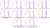 |
Fig. A.4. Same as Fig. A.2, but for the [O III] emission line. |
| In the text | |
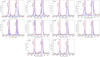 |
Fig. A.5. Same as Fig. A.3, but for the [O III] emission line. |
| In the text | |
|
Fig. B.1. ALMA CO(2−1) integrated-intensity map of NGC 5643 produced from the natural-weight data cube. The map is shown on a linear color scale. Black contours corresponds to the CO(2−1) emission map. They are shown on a logarithmic scale with the first contour at 8σ and the last contour at 2.2 × 10⁻¹⁷ erg s−1 cm2 beam−1. The various boxes correspond to the regions we selected to measure the two main spiral arms (see Sect. 5.3). Black boxes indicate regions that were selected as symmetric at either side of the nucleus. White boxes correspond to the supplementary regions to take additional individual CO(2−1) clumps into account. The diagonal solid red line indicates the separation axis between the two arms. North is up and east is left, and offsets are measured relative to the AGN. |
| In the text | |
|
Fig. C.1. Observed molecular and ionized gas properties. Top left panel: profile of the mass outflow. Top right panel: profile of the mass outflow rate. Bottom left panel: kinematic power profile of the outflow. Bottom right panel: momentum profile of the outflow. Orange squares and green circles correspond to the molecular and ionized outflow gas phases. The two regions to the east of the AGN (negative d − dAGN values) with no molecular outflow derived properties correspond to regions with cleared CO(2−1) emission. |
| In the text | |
|
Fig. D.1. Spatially resolved properties of the ionized (green circles) and molecular (blue squares) phases of the outflow: outflowing mass (top left), mass outflow rate (top right), outflow kinetic power (bottom left), and outflow momentum (bottom right). Blue squares and green circles correspond to the molecular and ionized outflow gas, respectively. The two regions to the east of the AGN (negative d − dAGN values) with no molecular outflow derived properties correspond to regions with cleared CO(2−1) emission. |
| In the text | |
|
Fig. D.2. Total outflow properties. Top left panel: outflow mass rate as a function of the AGN luminosity. The dashed orange and solid green lines are the best-fit correlations derived by Fiore et al. (2017) for the molecular and ionized gas, respectively. Top right panel: same as the top left panel, but for the outflow kinetic power. Solid, dashed, dotted, and dash-dotted lines represent Ėkin = 1.0,0.1,0.01,0.001 Lbol. Bottom panel: kinetic coupling efficiencies. The various horizontal lines correspond to theoretical values (Costa et al. 2018; Di Matteo et al. 2005; Dubois et al. 2014; Hopkins & Elvis 2010; Schaye et al. 2015; Weinberger et al. 2017). Blue stars and green squares represent the values derived in this work for the molecular and ionized phase of NGC 5643, respectively. The black circle shows the total kinetic coupling efficiencies for both (ionzed and molecular) gas phases. Brown hourglass and blue circles are adopted from Fiore et al. (2017) for the molecular and ionized phase, respectively, and the purple triangles are taken from Baron & Netzer (2019) for ionized outflows. We have consistently applied the same method as in Fiore et al. (2017) for the total ionized gas mass, |
| In the text | |
Current usage metrics show cumulative count of Article Views (full-text article views including HTML views, PDF and ePub downloads, according to the available data) and Abstracts Views on Vision4Press platform.
Data correspond to usage on the plateform after 2015. The current usage metrics is available 48-96 hours after online publication and is updated daily on week days.
Initial download of the metrics may take a while.