| Issue |
A&A
Volume 631, November 2019
|
|
|---|---|---|
| Article Number | A3 | |
| Number of page(s) | 21 | |
| Section | Interstellar and circumstellar matter | |
| DOI | https://doi.org/10.1051/0004-6361/201834903 | |
| Published online | 11 October 2019 | |
Multi-scale analysis of the Monoceros OB 1 star-forming region
II. Colliding filaments in the Monoceros OB1 molecular cloud★
1
Institut UTINAM – UMR 6213 – CNRS – University of Bourgogne Franche Comté, France, OSU THETA,
41bis avenue de l’Observatoire,
25000
Besançon,
France
e-mail: This email address is being protected from spambots. You need JavaScript enabled to view it.
2
Department of Physics, University of Helsinki,
PO Box 64,
00014,
Finland
3
IRAP, Université de Toulouse, CNRS, UPS, CNES,
31400
Toulouse,
France
4
Yunnan Observatories, Chinese Academy of Sciences,
396 Yangfangwang,
Guandu, Kunming,
650216,
PR China
5
Chinese Academy of Sciences, South America Center for Astrophysics (CASSACA),
Camino El Observatorio 1515,
Las Condes,
Santiago,
Chile
6
Departamento de Astronomía, Universidad de Chile,
Las Condes,
Santiago,
Chile
7
Shanghai Astronomical Observatory, Chinese Academy of Sciences,
80 Nandan Road,
Shanghai
200030,
PR China
8
Korea Astronomy and Space Science Institute,
776 Daedeokdaero,
Yuseong-gu,
Daejeon
34055,
Republic of Korea
9
East Asian Observatory,
660 N. A’ohoku Place,
Hilo,
HI
96720,
USA
10
Astrophysics Research Institute, Liverpool John Moores University,
IC2, Liverpool Science Park, 146 Brownlow Hill,
Liverpool
L3 5RF,
UK
11
University of Science & Technology,
176 Gajeong-dong,
Yuseong-gu,
Daejeon,
Republic of Korea
12
Academia Sinica, Institute of Astronomy and Astrophysics,
Taipei,
Taiwan
13
National Astronomical Observatory of Japan, National Institutes of Natural Sciences,
2-21-1 Osawa,
Mitaka,
Tokyo
181-8588,
Japan
14
SOFIA Science Centre, USRA, NASA Ames Research Centre,
MS N232-12 Moffett Field,
CA
94035,
USA
15
Department of Physical Science, Graduate School of Science, Osaka Prefecture University,
1-1 Gakuen-cho, Naka-ku, Sakai,
Osaka
599-8531,
Japan
16
Department of Physics, School of Science and Humanities,
Kabanbay batyr ave, 53,
Nur-Sultan
010000,
Kazakhstan
17
Eötvös Loránd University, Department of Astronomy,
Pázmány Péter sétány 1/A,
1117,
Budapest,
Hungary
18
Department of Earth Science and Astronomy, Graduate School of Arts and Sciences, The University of Tokyo,
3-8-1 Komaba,
Meguro,
Tokyo
153-8902,
Japan
19
Institute of Physics I, University of Cologne,
Zülpicher Str. 77,
50937,
Cologne,
Germany
20
AIM, CEA, CNRS, Université Paris-Saclay, Université Paris Diderot,
Sorbonne Paris Cité,
91191
Gif-sur-Yvette,
France
21
ICC, University of Barcelona,
Marti i Franquès 1,
08028
Barcelona,
Spain
22
Konkoly Observatory of the Hungarian Academy of Sciences,
1121 Budapest,
Konkoly Thege Miklósút
15-17,
Hungary
23
IAPS – INAF,
via Fosso del Cavaliere 100,
00133,
Rome,
Italy
24
Kavli Institute for Astronomy and Astrophysics, Peking University,
5 Yiheyuan Road,
Haidian District,
Beijing
100871,
PR China
25
European Southern Observatory (ESO) Headquarters,
Karl-Schwarzschild-Str. 2,
85748
Garching bei München,
Germany
Received:
17
December
2018
Accepted:
26
August
2019
Abstract
Context. We started a multi-scale analysis of star formation in G202.3+2.5, an intertwined filamentary sub-region of the Monoceros OB1 molecular complex, in order to provide observational constraints on current theories and models that attempt to explain star formation globally. In the first paper (Paper I), we examined the distributions of dense cores and protostars and found enhanced star formation activity in the junction region of the filaments.
Aims. In this second paper, we aim to unveil the connections between the core and filament evolutions, and between the filament dynamics and the global evolution of the cloud.
Methods. We characterise the gas dynamics and energy balance in different parts of G202.3+2.5 using infrared observations from the Herschel and WISE telescopes and molecular tracers observed with the IRAM 30-m and TRAO 14-m telescopes. The velocity field of the cloud is examined and velocity-coherent structures are identified, characterised, and put in perspective with the cloud environment.
Results. Two main velocity components are revealed, well separated in radial velocities in the north and merged around the location of intense N2H+ emission in the centre of G202.3+2.5 where Paper I found the peak of star formation activity. We show that the relative position of the two components along the sightline, and the velocity gradient of the N2H+ emission imply that the components have been undergoing collision for ~105 yr, although it remains unclear whether the gas moves mainly along or across the filament axes. The dense gas where N2H+ is detected is interpreted as the compressed region between the two filaments, which corresponds to a high mass inflow rate of ~1 × 10⁻³ M⊙ yr−1 and possibly leads to a significant increase in its star formation efficiency. We identify a protostellar source in the junction region that possibly powers two crossed intermittent outflows. We show that the H II region around the nearby cluster NCG 2264 is still expanding and its role in the collision is examined. However, we cannot rule out the idea that the collision arises mostly from the global collapse of the cloud.
Conclusions. The (sub-)filament-scale observables examined in this paper reveal a collision between G202.3+2.5 sub-structures and its probable role in feeding the cores in the junction region. To shed more light on this link between core and filament evolutions, one must characterise the cloud morphology, its fragmentation, and magnetic field, all at high resolution. We consider the role of the environment in this paper, but a larger-scale study of this region is now necessary to investigate the scenario of a global cloud collapse.
Key words: ISM: clouds / stars: formation
The reduced datacubes (FITS files) of our IRAM and TRAO observations are only available at the CDS via anonymous ftp to cdsarc.u-strasbg.fr (130.79.128.5) or via http://cdsarc.u-strasbg.fr/viz-bin/cat/J/A+A/631/A3
© J. Montillaud et al. 2019
 Open Access article, published by EDP Sciences, under the terms of the Creative Commons Attribution License (http://creativecommons.org/licenses/by/4.0), which permits unrestricted use, distribution, and reproduction in any medium, provided the original work is properly cited.
1 Introduction
Understanding star formation is a central challenge in astrophysics, impacting the physics and chemistry of the interstellar medium (ISM), stellar physics, as well as the evolution of galaxies and their stellar populations. A wealth of studies have been conducted to characterise star formation from the sub-parsec scales (where the ultimate gravitational instability turns prestellar cores into protostars) to galactic scales (where the large-scale dynamics shapes the distribution of giant molecular clouds) by way of the molecular cloud scale whose dynamics give birth to filaments and cores. At all scales the challenge is to untangle the complex interplay between gravity, turbulence, and the magnetic field. Additionally, the stakes are raised by the fact that various scales are coupled through non-linear processes, such as dynamical instabilities, supernovae explosions or ionisation, and photodissociation fronts.
Impressive progress has been made in the last few decades in the spatial resolution of star formation simulations, enabling the modelling of several orders of magnitude of physical scales in a single run. Renaud et al. (2013) modelled the hydrodynamics of a full Milky Way-like galaxy down to 0.05 pc, revealing how the spiral arms pump turbulent energy into the gas and determine the space and mass distributions of molecular clouds. They conclude that gravitation can govern the hierarchical organisation of structures from the galactic scale down to a few parsecs. This is in line with the “hierarchical gravitational collapse”, a scenario Vázquez-Semadeni et al. (2009, 2019) propose in which small-scale infall motions occur within large-scale ones, driving the dynamics and morphology of star formation regions. This dynamic view of a global collapse is particularly invoked for the formation process of high-mass stars, as supported by a number of observational studies (Schneider et al. 2010; Csengeri et al. 2011, Traficante et al.; 2018b, and the review by Motte et al. 2018). In contrast, Padoan et al. (2017; and references therein) propose that turbulent fragmentation, where supersonic turbulence is predominantly driven by supernovae explosions, determines the evolution and fragmentation of star formation regions.
Disentangling scenarios such as these requires one to accurately characterise the dynamics of star-forming regions from the core scale (~0.1 pc) to the molecular complex scale (a few tens pc), and to identify the structures and their origin in relation with the rest of the molecular complex. Molecular line observations are best suited to study the dynamics of molecular clouds, and, due to instrumental limitations, such studies often restrict their analysis to the scales probed by a given instrument to the chosen target. However, it has become increasingly common that ISM studies combine instruments with various angular resolutions (Csengeri et al. 2016; Liu et al. 2018a), in particular with the advent of interferometric facilities (Henshaw et al. 2017; Hacar et al. 2018). Another strategy consists in using very large high-resolution observational programmes to access several scales simultaneously (Pety et al. 2017; Nakamura et al. 2017; Sun et al. 2018). However, multi-scale studies remain scarce in the context of the early phases of star formation, and we are far from having a representative sample of molecular complexes where the nature and history of the most prominent structures would be understood.
Another limitation to progress in the understanding of star formation could result from the lack of diversity in the target selection. The Planck team has taken advantage of the excellent sensitivity and all-sky coverage of the Planck telescope between 30 and 857 GHz (Tauber et al. 2010) to compile the first all-sky, unbiased catalogue of candidate star-forming regions, the Planck Galactic cold clump catalogue (PGCC, Montier et al. 2010; Planck Collaboration XXIII 2011; Planck Collaboration XXVIII 2016). Several hundred PGCCs have been followed-up with the Herschel observatory in the frame of the open time key programme Galactic cold cores (GCC, Juvela et al. 2012), with an unbiased target selection strategy in terms of Galactic longitude and latitude, distance and mass, and leading to a sample of great diversity (Montillaud et al. 2015). The PGCCs were further followed-up by several projects. The “SMT All-sky Mapping of PLanck Interstellar Nebulae in the Galaxy” (SAMPLING) survey (Wang et al. 2018) is an ESO public survey of PGCCs in 12CO and 13CO (J = 2–1). The first data release contains 124 fields with an effective resolution of 36′′, a channel width of 0.33 km s−1 and an rms noise of Tmb < 0.2 K. The TOP-SCOPE project (Liu et al. 2018a) combines the “TRAO Observations of PGCCs” (TOP) science key programme of the Taeduk Radio Astronomy Observatory (TRAO), a survey of the J = 1–0 transitions of 12CO and 13CO towards ~ 2000 PGCCs, and the “SCUBA-2 Continuum Observations of Pre-protostellar Evolution” (SCOPE), a large programme at the JCMT telescope targeting the 850 μm continuum of ~1000 PGCCs (Eden et al. 2019).
In Montillaud et al. (2019, hereafter Paper I), we reported the analysis of the dense core population in the star-forming region G202.3+2.5,a complex filament at the edge of the Monoceros OB1 molecular complex and part of the GCC Herschel follow-up. We selected this target because of (i) its complex, ramified morphology, suggestive of a complex dynamics, (ii) its significant star formation activity as evaluated by Montillaud et al. (2015) and (iii) its location near the well studied open cluster NGC 2264 whose impact on the evolution of G202.3+2.5 needs to be investigated. In the present paper, the second in this series, we report the analysis of the relationship between the dynamics and star formation activity in G202.3+2.5. To conduct this study, we analyse the dust emission in the far-IR observed by Herschel and in the mid-IR by WISE on a 0.5 deg2 area covering a physical length of ~10 pc along the filament. This is combined with the molecular gas emission observed in the millimetre range with both the IRAM 30-m telescope, for high angular and spectral resolutions (~ 25′′ and 0.06 km s−1) in a limitedarea, and the TRAO 14-m telescope, in a larger area but with lower resolutions.
With this dataset, we now make a second step in the multiscale analysis of this region, covering from the core scale (~ 0.1 pc) to the filament scale (~10 pc). We analyse the density and thermal structure of the cloud from its dust and gas emissions, and correlate them with the distribution of cores whose characteristics were derived from their IR spectral energy distribution (SED) and molecular line emission in Paper I. The velocity field is examined and separated in different components which are used to infer the evolution of the cloud in conjunction with its environment.
The paper is structured as follows. The Mon OB 1 region is presented in the next part of this introduction. In Sect. 3 we present the observational data set used in this study. The methods are explained in Sect. 4. Section 5 gathers the factual results on the cloud structure, the core characteristics and the velocity field. These results are interpreted in terms of the evolution of the cloud in Sect. 6. Section 7 summarises our study.
2 The Monoceros OB1 molecular complex
The Monoceros OB1 molecular complex is a massive (3.7 × 10⁴ M⊙) and relatively evolved (>3 Myr) star formation region (Dahm 2008) located 760 pc from the Sun in the approximate direction of the Galactic anti-centre. Thanks to this location, this sky region is almost devoid of foreground and background emissions, with the exception of a few background clouds which belong to the Perseus Galactic arm more than 1 kpc farther, and can be identified from their radial velocities (~ 20−40 km s−1, Oliver et al. 1996), significantly greater than those of the Monoceros OB1 molecular complex (~ 0−10 km s−1).
Next to the centre of the eastern part of this region lays the open cluster NGC 2264 which contains more than 1000 members, the brightest of which is the O7 V multiple star S Monocerotis (S Mon). Along with several early B-type stars, they form the Mon OB1 association and are responsible for a vast Hα halo with ~ 1.5 degree in radius (20 pc) around NGC 2264 (blue area in Fig. 1). The Hα survey by Dahm & Simon (2005) revealed a population of several hundreds of T Tauri stars with ages scattered between 0.1 and 5 Myr, indicating a sustained star formation activity. Numerous embedded IR sources indicate that this activity is continuing. The first reported IR sources are IRS-1, or Allen’s source (Allen 1972), a 9.5 M⊙ B2 zero-age main sequence star next to the Cone Nebula (Williams & Garland 2002), and IRS-2, an embedded cluster of protostars 6′ north of IRS-1 (Sargent et al. 1984; Williams & Garland 2002). The active star formation within the region has been demonstrated by numerous identifications of outflows and Herbig–Haro objects from millimetre observations of molecularemission (Margulis et al. 1988; Schreyer et al. 1997; Wolf-Chase et al. 2003) and narrow-band imaging of atomic lines (Ogura 1995; Reipurth et al. 2004b), as well as infall motions (Peretto et al. 2006). More recently, several thousand young stellar object (YSO) candidates were identified from Spitzer observations of Mon OB1 east (Rapson et al. 2014), and tens of starless and protostellar dense cores were identified in a 0.6 deg2 field in the northern part of the cloud from sub-millimetre Herschel observations (Montillaud et al. 2015).
In projection, NGC 2264 appears superposed on a wide (15′ –30′, corresponding to 3–6 pc) elongated molecular cloud which extends over more than 2 degrees (> 25 pc), as revealed, for example, by the sub-millimetre emission observed by the Planck satellite at 857 GHz (red structure in Fig. 1) or by the large scale 13CO map presented by Reipurth et al. (2004a; their Fig. 7). This latter map suggests a complex dynamics of the gas, but the low spatial and spectral resolutions (100′′ and 0.6 km s−1, respectively) prevent one from a detailed analysis.
Rapson et al. (2014) showed that YSOs are distributed all over the molecular complex, with most objects concentrated in NGC 2264, and the remainder following mostly the shape of the elongated molecular cloud. From the distributions of the various classes of YSOs in the cloud, they conclude that star formation in the Mon OB1 east molecular cloud is heterogeneous, with the star formation in the cloud being more recent than that in NGC 2264. An even older, more dispersed population of stars may explain the large number of Class III objects in the region. Overall, this can be summarised as a gradient in star formation activity, which peaks in the open-cluster NGC 2264 and systematically decreases towards the northern part of the complex.
So far, most attention has been devoted to the brightest locations of the region, namely the open cluster NGC 2264, IRS-1 and IRS-2, and the sources in their close surroundings. In the present paper, we focus on G202.3+2.5, the northern tip of the Mon OB1 east molecular cloud, where Montillaud et al. (2015) report an active but recent star formation activity, and a complex morphology.
 |
Fig. 1 Three-colour composite image of Monoceros OB1 molecular complex. Red: Planck 857 GHz; green: WISE 12 μm from Meisner & Finkbeiner (2014); blue: Hα. The white and yellow contours are the footprints of Herschel SPIRE, IRAM, and TRAO observations, as labelled. |
3 Observations
3.1 Herschel observations
The cloud G202.3+2.5 was mapped with the instruments SPIRE (Griffin et al. 2010, 250, 350 and 500 μm,) and PACS (Poglitsch et al. 2010, 100 and 160 μm,) onboard the Herschel space observatory, as part of the Herschel open time key programme Galactic cold cores (Juvela et al. 2010). The characteristics and reduction steps for these maps are presented in detail in the GCC papers (see for example Juvela et al. 2012). The map resolutions are 18′′, 25′′ and 37′′ for the 250, 350 and 500 μm bands of SPIRE, and of 7.7′′ and 12′′ for the 100 and 160 μm bands of PACS. The calibration accuracies of the Herschel SPIRE and PACS surface brightness are expected to be better than 71 and 10%2, respectively.
Detected lines in our IRAM observations.
3.2 TRAO observations
Large-scale maps of G202.3+2.5 were obtained in April 2017 with the 14-m telescope of the TRAO as part of the Key Science Program named TOP (PI: Tie Liu). The SEQUOIA-TRAO, a multi-beam receiver with 4 × 4 pixels, was operated at 110.2 GHz with a spectral resolution of ~ 0.04 km s−1 and a beam size of 47′′, to observe the 13CO (J = 1–0) rotational transition. After smoothing the spectra to an effective resolution of 0.3 km s−1, the achievedsensitivity is rms K.
K.
3.3 IRAM observations
Part of the G202.3+2.5 cloud was observed with the IRAM 30-m telescope during March 2017. We observed this region at the frequency of 110 GHz with the EMIR receiver to record the lines of 13CO (J = 1–0) and C18O (J = 1–0). This front-end was connected to the VESPA autocorrelator configured to provide a spectral resolution of 20 kHz, corresponding to 0.055 km s−1 at 110 GHz. The FTS autocorrelator was also connected in parallel with a spectral resolution of 200 kHz, enabling us to detect additional lines including the 12CO (J = 1–0), CS (J = 2–1) and N2H+ (J = 1–0) lines. Table 1 summarises the observations.
We observed 14 tiles of typically 200′′ × 180′′ (i.e. 10 arcmin2), and built a mosaic which covers some 130 arcmin2 around the position  ′ 27′′). Each tile was observed multiple times and in orthogonal directions in on-the-fly (OTF) mode and position switching mode, with a scan velocity of at most 9′′ /s, a dump time of 1 s and a maximum row spacing of 12′′. The beam FWHM ranges from 21′′ at 115 to 26′′ at 93 GHz. The off position was observed every 1 to 1.5 min. It was chosen at
  (6h42m30.36s, + 10°33′ 21.2′′), after searching the SPIRE 250 μm map for a minimum in surface brightness (30.7 MJy sr−1, to be compared to the values in the range 100–5000 MJy sr−1 in the observed area). Pointing corrections and focus corrections were preformed every 1.5 and 3 h, respectively, leading to a pointing accuracy measured to be ≲ 5′′. We converted the antenna temperature to main beam temperature assuming a standard telescope main beam efficiency3 of 0.78 for CO observations and 0.80 for CS and N2H+.
3.4 Other observations
The previous data sets are complemented with archival data. Large scale Hα emission at 656 nm from the composite full-sky map by Finkbeiner (2003) is used in Fig. 1 and in Sect. 6. In the same section we also make use of the Second Digitized Sky Survey (DSS, McLean et al. 2000) in blue (λ = 471 nm), originating from the Palomar Observatory – Space Telescope Science Institute Digital Sky Survey. The resolution is better than 2′′, and data are given in scaled densities.
In the mid-IR domain, we used data from the Wide-Field Infrared Survey Explorer (WISE) satellite (Wright et al. 2010). It has four bands centred at 3.4, 4.6, 12, and 22 μm with spatial resolution ranging from 6.1′′ at the shortest wavelength to 12′′ at 22 μm. We used these data to complement the SEDs of cores in the mid-IR range. The data were converted to surface brightness units with the conversion factors given in the explanatory supplement (Cutri et al. 2011). The calibration uncertainty is ~6% for the 22 μm band and less for the shorter wavelengths.
4 Method
4.1 Dust temperature and column density
The three SPIRE maps were combined, as in Montillaud et al. (2015), to compute maps of dust temperature Tdust and column density N(H2), with an accuracy better than 1 K in Tdust in cold regions, corresponding to ~20% in column density at 15 K (Juvela et al. 2012). PACS data at shorter wavelengths were not included in the calculation because they may bias the column density estimate due to the contribution of stochastically heated grains (Shetty et al. 2009a,b; Malinen et al. 2011; Juvela et al. 2013). In G202.3+2.5, this seems particularly relevant since Tdust remains below 15 K except in the lowest column density regions outside the filaments, and at two very compact locations corresponding to young stellar sources.
To compute the Tdust and N(H2) maps, the SPIRE maps were convolved to a resolution of 38.5′′, slightly greater than that of the 500 μm map and reprojected on the same grid. For each pixel, the spectral energy distribution (SED) was fitted by a modified black-body function:
 (1)
(1)
where Bν(Tdust) is the Planck function at temperature Tdust, and the spectral index β was kept at the fixed value of 2.0.
The column density was then derived using the formula
 (2)
(2)
where mH is the mass of the hydrogen atom, μH2 = 2.8 is the mean particle mass per hydrogen molecule, and  is the dust opacity suitable for high density environments (Beckwith et al. 1990).
The maps of Tdust and N(H2) obtained with this method are shown in Fig. 2.
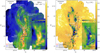 |
Fig. 2 Left: column density of molecular hydrogen in G202.3+2.5 as derived from SPIRE bands, assuming a modified black-body SED with fixed β = 2. Right: dust temperature in G202.3+2.5 derived from the same SED fitting. In both frames, the dark-blue solid line shows the footprint of our IRAM OTF observations, and the ellipses show the location, size (full-width at half-maximum of a Gaussian fit) and orientation of the submillimetre compact sources extracted by Montillaud et al. (2015). The regions defined in the main text are indicated with white shapes. In both frames, the inset shows a zoom to the junction region (white rectangle). |
4.2 Analysis of the molecular line data
4.2.1 Line fitting
We computed pixel-by-pixel Gaussian fits of the entire IRAM maps. For each map independently, a first fit was donewith a single Gaussian function. If the residuals showed features with signal-to-noise ratio (S/N > 5), a new fit was tested with a two-component Gaussian function. Again, when the residual features had S/N > 5, a three-component Gaussian fit was performed. This method is a simplified version of the one adopted in Paper I for individual sources. The simplification was motivated by the large number of spectra to be fitted (several thousand spectra). Asshown in Sect. 5.2, this is not sufficient for a few sightlines where up to four velocity components are seen. Still, we did not discard the few sightlines where a fourth component appears since for the vast majority of sightlines, only one or two components dominate the spectra and were sufficiently well fitted (examples of the most complex spectra in this field are shown in Fig. 8) for the general analysis of velocity components.
4.2.2 Temperature and density calculations
We calculated the excitation temperatures Tex and column densities of 13CO and C18O following the method described by Wilson et al. (2013). We present our calculations in detail in the Sect. A.2 of our Paper I. In short, we assume that the 12CO (1–0) line is optically thick. It appears as a reasonable assumption since the H2 column density is ≳3 × 1021 cm−2 in the area mapped with the IRAM 30-m (Fig. 2). This enables us to compute directly, for each pixel, the excitation temperature of this line from its maximum Tmb. We then assumed that the J = 1–0 transition of all the CO isotopologues have the same excitation temperature, so that we could derive the optical depths of 13CO (1–0) and C18O (1–0), and therefore the column densities of 13CO and C18O. The validity of this latter assumption is limited by the fact that the three transitions tend to probe different layers in the cloud. We present and discuss the column density maps in Sect. 5.1.3.
4.3 Velocity-coherent structures
We investigated the velocity-coherent structures in G202.3+2.5 as traced from the emission of CO isotopologues. We implemented a similar method as the FIVE algorithm developed by Hacar et al. (2013). Contrary to these authors, who analysed the emission of dense gas tracers (C18O and N2H+ in Hacar et al. (2013), N2H+ and NH3 in Hacar et al. 2017), we focus on moderate density tracers (13CO and C18O) for the following reasons. At 760 pc, G202.3+2.5 is farther than the clouds studied by Hacar and coworkers: 238 pc for NGC 1333 (Hacar et al. 2017) and 150 pc for Musca (Hacar et al. 2016). This implies that the dense structures are not as well resolved as in those studies. On the other hand, this greater distance enables us to cover a larger area, an asset to study the large scale dynamics in the cloud. CO isotopologues trace the appropriate densities to analyse the connections between the different large structures in the cloud.
As the first step, we convolved each plane of the data cubes with a Gaussian kernel with a FWHM of 25′′ to improve the S/N. For each pixel with a spectrum peaking at values with S/N > 6, we used the central velocity of each Gaussian component of the fits presented in Sect. 4.2.1 to build a cube of discrete points in the position-position-velocity space.
We used a friends-of-friends algorithm to connect the most related points and identify the coherent structures. For a given selected pixel, the neighbours in a box of 5 × 5 pixels and five channels were examined, corresponding to a maximum radius of two cells around the selected pixel in each axis. The box size, corresponding to 25′′ (~0.1 pc), is similar to the beam size, securing the spatial coherence of the structure. Similarly, five channels correspond to 0.3 km s−1, which is typically the width of the most narrow lines in 13CO and C18O, securing thevelocity coherence of the structure. The cells with a S/N > 6 were considered friends of the selected pixel. The method was iterated by considering each new friend as the new selected pixel, until no new friend was found. We present the results in Sect. 5.2.
5 Results
5.1 The physical structure of G202.3+2.5
5.1.1 Dust column density and temperature maps
Figure 2 shows the distributions of the molecular hydrogen column density N(H2) and the dust temperature derived from Herschel observations with a resolution of 38.5′′, corresponding to ~0.15 pc at the distance of 760 pc. It reveals the complex and ramified structure of G202.3+2.5, with two relatively broad (~ 0.5 pc), cold (Tdust < 14 K), and dense (N(H2) ≳ 5 × 1021 cm−2) filaments at δ > 10°45′ (hereafter the north-western and north-eastern filaments) joining into an even broader (~ 1 pc) and denser filamentary structure at δ < 10°45′ (hereafter the main filament; these structures are shown in the left frame of Fig. 2).
The peak column density and lowest (line-of-sight average) temperature in the field are reached at the junction of the filaments with values N(H2) ≈ 5 × 1022 cm−2 and Tdust ≈ 11 K. This junction region hosts a wealth of compact sources, many of which are aligned along an arc-shaped ridge (the arc in Fig. 2), mostly aligned with the north-south direction. This region corresponds to the surroundings of the source labelled IRAS 27 or NGC 2264 H by Wolf-Chase et al. (2003) where they found evidence of an outflow. Interestingly, the peak Tdust of the field is also reached in this area with a value of Tdust ≈ 17 K, and is certainly an effect of the heating by the protostar responsible for the outflow. Just south of this source, a linear structure (the bar in Fig. 2) inclined from south-east to north-west joins the arc by its southernmost end, contributing to the complexity of this ramified structure.
A similar structure as that of NGC 2264 H is found at the southernmost end of the main filament, although with less contrasted values of Tdust = 13 and 17 K. This second source corresponds to the source labelled IRAS 25 or NGC 2264 O by Wolf-Chase et al. (2003), where they also found evidence of an outflow, and which Ogura (1995) identified as the object responsible for the giant Herbig–Haro object HH 124 (outside of the Herschel maps). These two objects are connected by the most central part, or core in the sense defined by Rivera-Ingraham et al. (2017), of the main filament, where column density is ≳ 1022 cm−2 and reaches values ~2 × 1022 cm−2 and temperatures Tdust ≲ 13 K at severalcompact locations.
The north-eastern filament exhibits a large arc-shaped and fragmented structure with column density generally ≲ 1022 cm−2, except at a few compact locations where this value is marginally exceeded.
The north-western filament is mostly composed of two regions: one large, dense, and cold clump (hereafter the north clump; top white ellipse in Fig. 2, right) at its northernmost end (α = 6:40:54, δ = 10:55:52) with N(H2) ≈ 2 × 1022 cm−2 and Tdust ≈ 12.5 K, and a more diffuse region which connects the north clump to the junction region. Despite relatively large values of column density (N(H2) ~ 3−10 × 1021 cm−2), this latter region (hereafter designated as “the bridge”, since it connects the north clump and the main filament, central white ellipse in Fig. 2, right) has temperature values of ~14.5 K, comparable to those of the immediate surroundings of the cloud and making the north clump look isolated from the rest of the cloud in the temperature map of Fig. 2.
From these column density values, we derive the total masses and linear masses of the main structures discussed above as summarised in Table 2. We did not attempt any automatised extraction of the filaments from the dust emission maps, since our molecular line observations reveal a more complex structure than suggested by the dust emission. We computed masses within column density contours of 2 × 1021 cm−2 and obtained values between 240 M⊙ for the bridge and 2100 M⊙ for the southern part of the main filament. The junction region and the southern part of the main filament gather 3900 M⊙, that is ~ 60% of the cloud mass in the map. Table 2 also lists approximate estimates of the physical length of these structures, from which we derived linear masses between 120 and 230 M⊙ pc−1 in the northern filaments, and of 530 and 580 M⊙ pc−1 in the junction region and southern main filament. These values are much larger than the critical linear mass for gravitational instability under thermal support. Using  , where cs is the isothermal sound speed and G is the gravitational constant (Ostriker 1964), we obtain Mlin,crit = ~16−32 M⊙ pc−1 for a 10–20 K gas. However, turbulent and magnetic support can also contribute. We do not have constraints on the magnetic field strength in this paper, but in Paper I, we reported velocity dispersions
  km s−1 in the junction region and 0.2–0.4 km s−1 in the northern filaments. Replacing the sound speed by
  in Ostriker’s formula (Chandrasekhar 1951, see Appendix B) where σNT is the non-thermal velocity dispersion (Eq. (A.6) in Paper I), we find critical linear masses of Mlin, crit = 92−186 M⊙ pc−1 for the junction region and Mlin, crit = 37−92 M⊙ pc−1 for the northern filaments.
This implies that, unless the magnetic field plays a major role, all the filaments should be fragmenting. This picture is consistent with the numerous starless and protostellar cores identified everywhere along the filaments. However the low threshold of 2 × 1021 cm−2 includes gas that is widely scattered and eventually may not, or not quickly, be involved in star formation. A closer view of present or imminent star formation is obtained by considering a greater column density threshold of 8 × 1021 cm−2. This value corresponds approximately to an extinction of 8 mag, which is similar to the background extinction threshold of AV ~ 4−8 mag proposed by McKee (1989) and reported by Enoch et al. (2007; AV ~ 8 mag in Perseus) or André et al. (2010; AV ~ 10 mag in Aquila). It reveals that in the northern filament, only the north clump is clearly prone to star formation. With Mlin = 130 M⊙ pc−1, the main filament is also very active, but the junction region appears by far as the most active part of G202.3+2.5, with Mlin = 210 M⊙ pc−1.
Approximate lengths and masses of the main structures identified in the column density map.
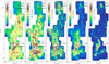 |
Fig. 3 Integrated intensity maps of the main detected lines in our IRAM observations. The sources s1454 (North clump) and s1446 (NGC 2264 H) are indicated in each frame. A scale bar is shown in frame a. The ellipses in frame b show the GCC sources with the same colour code as in Fig. 2: red for protostellar, blue for starless, and black for undetermined. The black and red squares in frame c show the areas where the average spectra in Fig. 5 were computed. The structures named “the arc” and “the bar” are shown in frame e. |
5.1.2 Average spectra and integrated intensity maps
All the transitions summarised in Table 1 are detected at least in the junction region. Figure 3 shows the velocity-integrated intensity maps of all the detected transitions in our IRAM dataset, except for C17O and C34S which are only weakly detected in the junction region ( and 0.4 K, respectively) and in the north clump (
 and 0.5 K, respectively, corresponding to S/N ~ 5). The integrated maps of C17O and C34S are shown in Fig. A.1. A wider view of the 13CO emission in the region is presented in Fig. 4, which shows the velocity-integrated map of the TRAO data.
The 12CO (J = 1–0) emission (Fig. 3a) fills the whole map with integrated intensities of the order of 50 K km s−1 and exceeding 100 K km s−1 around NGC 2264 H (s1446 in the GCC catalogue). It presents a morphology mostly similar to the one observed from dust emission, with the important exception of the north clump where significantly lower values of the integrated intensities are found (~ 30 K km s−1). This contrast in intensity between the north clump and the remainder of the field decreases when examining the emission of rarer CO isotopologues. Figure 5 compares the average spectra of the north clump and of a 2 arcmin square of the main filament (black and red squares, respectively, in Fig. 3c). It shows that the ratio of the peak Tmb of CO isotopologues in the main filament, Tmb(MF), to that in the north clump, Tmb(NC), decreases from Tmb(MF)∕Tmb(NC) ~ 2 for CO, to ~1 for 13CO, ~ 0.5 for C18O, and ~ 0.8 for C17O. Moreover the line width in the main filament is found to be about twice as large as that in the north clump for all isotopologues.
The region of the bar (Fig. 3e) appears as a continuous structure with a similar morphology for all the isotopologues (Figs. 3 a–c). In contrast, the arc region (Fig. 3e) shows different morphologies in all the CO maps, suggesting a complex structure along the line-of-sight with variations in excitation possibly related to the outflow reported by Wolf-Chase et al. (2003) and in Paper I.
As shown in Fig. 3d, the CS (J = 2–1) emission peaks at the location of NGC 2264 H with a peak value of 11.7 K km s−1. The general morphology of the CS integrated intensity map is similar to that of the C18O map, with (i) the junction region, and especially the arc which hosts NGC 2264 H and the bar, dominating the emission, (ii) the north clump showing relatively diffuse emission and (iii) the bridge not being detected. Differences are found in the arc, which appears more compact than in CO, and shows a bright extension to the north-east, and in the bar which appears fragmented in three clumps separated by ~1.5−2.0 arcmin (~0.35−0.45 pc). The C34S emission (Fig. A.1) is about ten times fainter than that of CS but shows almost exactly the same distribution.
The N2H+ (J = 1–0) emission traces the densest regions of the cloud and therefore is seen at quite compact locations (Fig. 3e). The arc around NGC 2264 H is very well traced by this transition with the map maximum value of 6.2 K km s−1 being reached at the location of NGC 2264 H. Another bright compact source appears in the same arc, 1.5 arcmin (~ 0.35 pc) south of NGC 2264 H with a peak value of 5.0 K km s−1. A 3-arcmin (0.7 pc) long, continuous portion of the arc is found with an intensity ≳ 2.5 K km s−1. The bar, southwards of the arc, is fragmented into at least three compact sources, even more clearly than in the CS map. The north clump is bright in N2 H+ with a peak integrated intensity of 4.0 K km s−1, and a significant emission (> 1.0 K km s−1) within a 2 × 1 arcmin elliptical region.
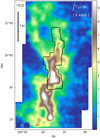 |
Fig. 4 Integrated intensity map of 13CO in our TRAO observations. The black line shows the footprint of the IRAM observations. A scale bar is shown in the top left corner. |
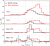 |
Fig. 5 Spectra of CO isotopologues in the north clump (black) and in the main filament (red). Spectra are averaged within 2 arcmin-wide square regions centred at (α, δ) = (6:40:54.9;+10:55:40.8) for the north clump and (α, δ) = (6:41:03.6;+10:34:28.7) for the main filament. In the C17O (J = 1–0) transition, the three vertical blue lines indicate the positions of the three hyperfine components assuming vlsr = 5.3 km s−1. |
5.1.3 Gas column density maps
Figure 6 compares the column density maps derived from IRAM observations as presented in Sect. 4.2.2. The same structures as seen in the dust column density map (Fig. 2) are visible in the 13CO and C18O column density maps, however with different contrasts. The values of  (frame a) range between 5.0 × 1015 cm−2 at the edge of the map and 5.3 × 1016 cm−2 at the peak of the junction region. To convert those values to H2 column densities, we assume aratio
  (e.g. Pineda et al. 2010) and we use the Galactic gradient in C isotopes reported by Wilson & Rood (1994) to compute the ratio
  for the galactocentric distance of G202.3+2.5 (9.11 kpc, Montillaud et al. 2015). We obtain N(H2) values between 3.8 × 10²¹ and 4.0 × 1022 cm−2.
In Fig. 6b we also present the column density map for C18O. The column density of N(C18O) reaches a maximum value of 6.6 × 1015 cm−2 in a different part of the junction region than 13CO. Assuming a ratio  (Wilson & Rood 1994), it corresponds to a N(H2) value of 4.1 × 1022 cm−2.
The N(H2) column density values obtained for 13CO and C18O are in good agreement with each other. This implies that 13CO emission is generally not sufficiently optically thick to strongly bias (underestimate) the 13CO column density measurement. Indeed, the peak values of τν derived from Eq. (A.1) in Paper I for 13CO are ~0.5 in the junction region, with maximum values of ~1 localised in compact sources. Only the north clump exhibits larger values of ~ 0.8 with a maximum τpeak = 1.3, despite column densities and peak Tmb being lower than in the southern area.
This is related to the trend discussed in Sect. 5.1.2 and shown in Fig. 5, where rarer isotopologues tend to be brighter in the north clump than in the junction region, while 12CO is fainter in the north clump than in the rest of the filament. Similar trends are observed in Fig. 6e, showing the integrated ratio of C18O/13CO cubes4, where the north clump has almost as high ratios as the junction region in spite of its fainter emission and lower column density. More striking is the map of  (Fig. 6c), where the largest values are found in the north clump (up to approximately two times the X18∕13 value given by Wilson & Rood 1994), and approximately three times larger than in the rest of the filament. Interestingly, the map of 12CO excitation temperature (Fig. 6d) reveals a strong contrast between the north clump (Tex ~ 12 K, morphology practically invisible), and the rest of the filament (Tex ~ 15−30 K, clear morphology which contrasts well with the background).
The reasons for this large difference in Tex between the north and south of the field are not fully clear. Apart from the north clump, the spatial variations in Tex show a morphology very similar to the one of  . Since Tex increases with increasing molecular hydrogen volume density (see, for example, Fig. 2.7 in Yamamoto 2017), and assuming that the
  map is a good proxy for volume density variations, at least part of the variations in Tex are likely to reflect variations in n(H2). Other possible effects contributing to these variations include a lower external heating in the north clump and optical depth effects for example as a result of differences in velocity dispersion.
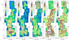 |
Fig. 6 Column density maps of 13CO (frame a) and C18O (frame b), and their ratio (frame c) normalised to the expected 13CO/C18O from Wilson & Rood (1994). Frame d: Excitation temperature of 12CO.
Frame e: Integrated |
5.2 Velocity components
The velocity structure of G202.3+2.5 is quite complex. Figure 7 shows that in 13CO several velocity components are overlaid along most sightlines, with a scatter in velocity greater than 4 km s−1, and fluctuations in velocity within each component of ~ 3 km s−1 in the junction region (offset <540′′), ~ 3 km s−1 around the bridge (offsets between 540 and 1300′′), and < 0.5 km s−1 in the north clump (offset > 1300′′). This complexity is even greater at some positions, as shown in Fig. 8, where up to four different velocity components are found.
Figure 9 shows the 13CO channel maps of G202.3+2.5 from TRAO and IRAM data, as well as the 12CO channel maps from IRAM data. TRAO data reveal that the north-eastern and north-western filaments (including the north clump) are parts of the same large structure which appears as an elongated loop at velocities between 4 and 6 km s−1. Both TRAO and IRAM data show that between 6 and 8 km s−1 the emission of the filament is dominated by the junction region and the main filament, and that at 6 km s−1 the brightest part of this structure is in the junction region, confirming that there is a continuity from the north-eastern and north-western filaments to the main filament. At larger velocities (vlsr ≳ 7.5 km s−1), the main filament continuously extends to the north west, up to the region of the bridge. Interestingly, although in 13CO the north clump seems brighter than the bridge, in the IRAM 12CO channel maps the situation is reversed. The channel maps of the other tracers detected with the IRAM telescope are shown in Appendix A.
Another view of the velocity structures is presented in Fig. 10 which shows the line centroids obtained from our 13CO and C18O cubes. The 13CO frame reveals multiple interconnected components and large-scale velocity gradients. The lower point density in the C18O centroid distribution unveils the skeleton of the cloud, with a clear large-scale velocity gradient in the north-south direction, and a more confused east-west gradient in the junction region.
Figure 11 shows the result of the friends-of-friends identification of 13CO velocity-coherent structures (VCS). Five major structures are identified, three in the junction region (VCS 1-3), the two others corresponding to the north clump (VCS 5) and the bridge (VCS 4, between the north clump and the junction region). The north clump appears as a single structure at ~ 5 km s−1 relatively unattached to the junction region. The bridge, which seems to connect the north clump to the junction region in Herschel maps, turns out to be completely disconnected in velocity from the north clump, and presents velocities similar to the reddest ones in the junction region, as well as a significant velocity gradient of ~ 0.3 km s−1 arcmin−1 (=1.5 km s−1 pc−1). The yellow structure (VCS 3) in the PPV diagram of Fig. 11 a has similar velocities as the bridge and its morphology in the plane of the sky suggests that it could be its continuation southwards. It strongly overlaps (in the plane of the sky) with the light blue structure (VCS 2) in Fig. 11a, which spans bluer velocities, from 5 km s−1 (as in the north clump), to ~ 7 km s−1 (the averagevelocity of the cloud). These two structures are well separated by a gap in velocity which oscillates along the north-south direction, as seen in the δ − v plane of Fig. 10 for 13CO, and are mostly connected via VCS 1 at the southernmost end of the IRAM map. This is particularly striking in the δ − v plane of Fig. 10 for C18O.
The second panel of Fig. 11 shows the same structures projected on the plane of the sky, with the average velocity of each VCS colour coded. This figure also shows the densest parts of the cloud as traced by the N2 H+ emission (hatched regions), for which we obtained the velocity of the isolated component using hyperfine structure line fitting. The dense part of the arc appears to be located along the edge of VCS 2 (the light-blue component), and next to VCS 1 (the light-red component). With average velocities of about 7.7, 7.3, and 6.3 km s−1 for VCS 1, the N2H+ emission of the arc, and VCS 2, respectively, the arc is also between VCS 1 and 2 along the velocity axis. The other notable N2 H+ emissions correspond to s1449 (vlsr = 7.56 km s−1), s1457 (vlsr = 7.81 km s−1), and s1454 (vlsr = 5.29 km s−1). Those sources are located in VCS 1 (vlsr = 7.7 km s−1), for s1449 and s1457, and VCS 5 (vlsr = 5.5 km s−1), for s1454, both spatially and in the velocity space.
Table 3 gives the main properties of the five largest 13CO velocity-coherent structures. Consistently with the results reported in Sect. 5.1.3 and Fig. 6, the north clump (VCS 5) stands out with a low average 13CO column density, a low scatter in 13CO brightness temperature and a low radial-velocity dispersion. This suggests that it belongs to a part of G202.3+2.5 with different environmental conditions than in the four other components. VCS 1-3 are all immediately next to the junction region and around the dense gas traced by N2 H+. They individually present large radial velocity ranges between Δvlsr ~ 1.7 and 1.9 km s−1 with large 13CO column densities (≳7 × 1021 cm−2). Finally, the impression given by Fig. 11 that VCS 4 (the bridge) is the northwards continuation of VCS 3 is supported by the similarity of their velocity dispersions, average and dispersion Tmb(13CO) and average 13CO column densities.
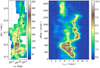 |
Fig. 7 Left: velocity integrated map of 13CO in K km s−1. Right: position-velocity diagram along the dashed line of the left frame. The two circles on the map in the left frame show the locations of the spectra shown in Fig. 8. |
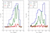 |
Fig. 8 Spectra of CO, 13CO and C18O (J = 1–0) in the junction (left) and bridge (right) regions at the locations marked by black circles in Fig. 7. The spectra of CO is divided by 2. The black dashed lines are the 3-component Gaussian fit of the 13CO lines (Sect. 4.2.1). |
6 Discussion
The goal of the paper is to investigate whether the dynamics of G202.3+2.5 shapes star formation in this cloud. In this section, we first investigate the outflows from the junction region. We then make an inventory of star formation activity in the cloud, and then show that the cloud is made of two colliding filaments. We end by discussing the role of triggering in this star formation region.
6.1 Outflows from the junction region
Outflows from NGC 2264 H (source 1446) have been detected by Wolf-Chase et al. (2003) from 12CO(2–1) observations, with a complex morphology which is not clearly bipolar (see their Fig. 9). Reipurth et al. (2004b) showed from Hα images that the Herbig–Haro objects HH 576 (on the north-west of NGC 2264 H) and HH 577 (on the south-west of NGC 2264 H) are at the end of flows that cross roughly at the location of this source (see their Fig. 7).
Our data enable us to characterise the outflows in the junction region with a better spatial resolution than Wolf-Chase et al. (2003). Figure 12 shows the 12CO(1–0) spectra in this region. The line profiles in frame b show that the bulk emission of the 12CO(1–0) line peaks near 7 km s−1, with a blue wing at vlsr ~ 0−5 km s−1, at the north-west edge of the source. When moving to the south-east, the bulk emission peak shifts towards 5 km s−1, while the blue wing disappears and a strongred wing grows between vlsr = 10 and 30 km s−1.
Frame a in Fig. 12 shows an N2H+ integrated intensity map of the junction region with red and blue contours of 12CO channel maps with velocities of the red and blue line wings, respectively. The red-wing emission is distributed along an east-west elongated structure, in a direction compatible with the flow towards HH 576. The blue wing contours are distributed in three blobs, hereafter referred to as BW1, BW2, and BW3 (Fig. 12a), exhibiting a lack of bipolar symmetry with the red contours.
Part of the asymmetry can be attributed to the large scale east-west velocity gradient. The bulk emission of source 1450, between −2 and +8 km s−1, makes the source appear in the contour plot despite the absence of blue wings. The suggestion by Wolf-Chase et al. (2003) that BW2 might be an outflow associated with their source 27S3 (s1450), is therefore irrelevant.
The location of BW1, at the north-west of source 1446, is mostly opposed to the elongated red-shifted emission on the south-east of source 1446. We follow Wolf-Chase et al. (2003) in interpreting them as a bipolar outflow from the protostellar source 1446. Hereafter, we will refer to this outflow as the main outflow. It was noted by Reipurth et al. (2004b) that the main axis of this outflow is well aligned with the flow towards HH 576.
The situation is more complex for BW3. It corresponds to no known dense sources in dust emission data. It presents a double peaked 12CO line at ~ 5 and 7 km s−1, but the 13CO line shows a single peaked line at ~ 7 km s−1, suggesting that the red peak (7 km s−1) traces the denser and less excited matter, while the blue peak (5 km s−1) arises from a more diffuse and excited component. Wolf-Chase et al. (2003) proposed that this blue-shifted emission is an outflow from their source 27S2 (s1448), whose red counterpart would be blended in velocity with the ambient matter, thus difficult to detect. However, (i) s1448 is not detected in N2 H+, an abundant species in protostellar cores, (ii) the shape of the BW3 contours is elongated in the direction of s1446, and (iii) the red contour at 11.4 km s−1 extends to the south-west of the source 1446, in a direction opposed to BW3, making it an interesting candidate for the red counterpart of BW3. Hence, this latter red emission and BW3 could be the two components of a secondary outflow from s1446. Overall, our data are compatible with the idea that both outflows originate from the source 1446, which should therefore be a system of (at least) two stars.
The map in Fig. 12 shows that the red-shifted emission of the main outflow is made of two parts: one ~ 100′′ long part from s1446 to the south-east, the other farther to south-east, spanning only ~ 50′′. They are visible in the position-velocity (PV) diagram of Fig. 12c, where they seem independent from each other, the first one being attached to s1446 (offset ~ 200′′), disconnected of the second one (offset ~ 100′′). If the two parts trace the same outflow from source 1446, the discontinuity in velocity between them remains to be explained.
The velocity gradient within the first part of the main outflow shows velocities of ~ 10 km s−1 near s1446, and ~ 20 km s−1 at distances ~ 100′′. Since the bulk velocity is ~ 7 km s−1, it means that the more distant gas flows faster, a fact in contradiction with the idea of a steady outflow, and suggesting that the outflow is ejected in an intermittent fashion. In this scenario, all the material in the first part of the outflow would have been ejected simultaneously, the faster parts of the gas reaching greater distances. The velocities and distances are compatible with this scenario: the gas traced by the contour at 24.6 km s−1 lays at ~ 100′′ from s1446, while the contour at 11.4 km s−1 traces gas typically within 25′′ of s1446. With a bulk velocity of 7 km s−1 and assuming that the inclination of the velocity vector with the sightline is the same for both components, one finds the same ratio between the angular distance and radial velocity Δθ∕Δvlsr ≈5.7′′/(km s−1), that is the same age. In addition, the association with the HH 576 object 6′ away (1.3 pc in projection) already makes HH 576 a giant Herbig–Haro object (Reipurth & Bally 2001; Reipurth et al. 1997). It is therefore unlikely that the outflow main axis is too far from the plane of the sky. Assuming an upper limit of 30 deg for this angle, the maximum radial velocities observed in the outflow of ~ 30 km s−1 (23 km s−1 relative to the source) correspond to ~ 50 km s−1 relative to the source, and the travel duration of the outflow is ~ 104 yr. This scenario also naturally explains the discontinuity in velocity of the second part of the outflow if it was ejected during a previous outburst event. From its distance (125′′) and its radial velocity (~ 10 km s−1) relative to the source, one derives an age of ~2 × 10⁴ yr.
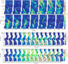 |
Fig. 9 Top: 13CO channel maps from TRAO data. Middle: 13CO channel maps from IRAM data. Bottom: 12CO channel maps from IRAM data. The channel velocities are written in the top corners. In the two first and last frames, the sources from the GCC catalogue are shown as white ellipses and the arc and bar regions are shown as white lines. The north clump and NGC 2264 H are labelled as “s1454” and “s1446” in TRAO maps, and “N” and “H” in IRAM maps, respectively.Scale bars are in the next to last frames. |
 |
Fig. 10 Distribution of line centroids in the position-position-velocity space for 13CO (left) and C18O (right). The colours vary with velocity to help the 3D visualisation. The black points are projections of the colour ones on the faces of the box. In the right frame, lines joining the projections to the colour points are drawn to help visualising in 3D the positions of s1454 (in the north clump), s1461 (at the root of the north-eastern filament), s1446 (in the arc), and s1453 (just north to the arc). |
6.2 Colliding filaments
6.2.1 Relative positions along the line of sight
The relative positions along the line of sight of the various velocity components and their position with respect to the rest of the Mon OB1 region cannot be determined solely from our millimetre observations. Extinction and scattering are better suited for this purpose. A 1° × 1° DSS2 blue map (λeff = 471 nm) of G202.3+2.5 is presented in Fig. 13, showing a strong gradient in the average surface brightness along the south-west to north-east direction. A surface brightness profile along this direction (Fig. 13d) reveals that this gradient presents two different slopes. The steeper one is in the area with values ≳5000 (arbitrary units), closer to the open cluster NGC 2264, and corresponds to the Hα emission (hereafter area 1, in blue in Fig. 1). It strongly suggests that the surface brightness is dominated by scattered light from the stars of NGC 2264 in this area, and by the field stars in the background and foreground of Mon OB1 in the rest of the field of view (hereafter area 2). This is summarised by a sketch in Fig. 14.
Interestingly, the densest part of the junction region, traced by the N2 H+ emission, is located just at the edge of area 1, but no structures seem to correspond in the DSS map. Instead, a relatively strong emission of scattered light with unrelated morphology is observed at this location. Because extinction is strong at this wavelength, it implies that the structure responsible for scattering is in front of the one traced by N2 H+.
In contrast, the north-eastern and north-western filaments appear clearly in the DSS map in extinction against the Galactic scattering background in area 2, forming structures which match very well the 13CO emission between 3.6 and 6 kms−1. However, the southernmost tip of the north-eastern filament, located next to the N2 H+ emission, is not seen in extinction. This is consistent with the idea that this 13CO emission and the N2H+ emission arise from different layers of the same structure located behind the scattering material.
Figure 13 also compares the morphology of the main filament, traced by the 13CO emission between 6.3 and 9.3 km s−1, with the DSS map. The southernmost end of the main filament fits closely the inner part of a large arc seen both in scattered light in the DSS map and in mid-IR emission at 12 μm (Fig. 1), a typical tracer of photo-dissociation regions (e.g. Pilleri et al. 2012; Anderson et al. 2014). In the first 15′ northwards of the arc, the main filament is straight and oriented radially with respect to NGC 2264. In this part of the filament, there is a relatively good match between the crest of the filament and a decrease in the DSS surface brightness, however with a lesser contrast than in the case of the north-eastern and north-western filaments. Considering that the column density in the main filament is 2− 3 times greater than in the northern filaments, it cannot be in front of the scattering material. It cannot be behind it either, since a decrease in scattered light is observed. We conclude that the main filament is part of the scattering material. In addition, the shape of the arc, possibly seen edge-on or slightly from the back, and the orientation of the filament suggest that its angle with the plane of the sky is small.
Gathering all these elements, we conclude that (i) the main filament is weakly inclined with respect to the plane of the sky and at a distance nearly equal to that of NGC 2264, (ii) it splits at the level of the junction region into one short filament corresponding to the bridge, and one larger structure stretching away from the observer, corresponding to the northern filaments.
Finally, we note that the result presented in Sects. 5.1.2 and 5.1.3 that the ratio between CO and 13CO brightness is larger in the main filament than in the north clump also suggests different environment conditions in the two structures. This could be naturally explained in the frame of our proposed geometry if the northern structures and the main filament used to be detached structures, and recently collided at the level of the junction region. We discuss further this idea in the following sections.
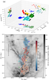 |
Fig. 11 Frame a: 3D position-position-velocity view of the velocity-coherent structures in 13CO. The pale colours are projections of the structures onto the plane of the sky, the α − v plane and the δ − v plane. Each colour corresponds to a different structure. The id numbers of the five components tabulated in Table 3 are indicated in the δ − v plane. Frame b: Thermal emission of dust in G202.3+2.5 at 250 μm (Herschel/SPIRE). Coloured regions show the same velocity-coherent structures as in frame a for 13CO J = 1–0 (no symbol) and N2H+ J = 1–0 (isolated component, with hatches). The colour scale shows the average radial velocity of each structure. Transparency reveals the overlaps between the structures. Sources 1446, 1449, 1454, and 1457 are indicated in black. The white lines show the arc and the bar. The coloured numbers indicate the five main VCSs. |
6.2.2 Collision and inflow
Adopting the geometry obtained in the previous section, the radial velocities of the main filament (including the bridge) and of the northern filaments imply that the two structures are moving towards each other with relative velocities of at least 2–4 km s−1.
This conclusion is strengthened by other elements. Figure 15 shows the central velocity of the isolated hyperfine component of the N2H+ emission in the junction region. There is a clear velocity gradient from ~ 5 km s−1 in the south-east edge to ~ 9 km s−1 in the northern edge of the emission, so that this region, which is the densest of the cloud both in terms of column and volume densities, is also the one with the steepest velocity gradient. This can also be seen from C18O emission in the right frame of Fig. 10. It is striking that the arc shape of the N2 H+ emission is also followed by the integrated emission of 13CO between 6.3 and 9.3 km s−1, corresponding to the main filament, and seems to wrap around the integrated emission of 13CO between 3.6 and 6.0 km s−1, which corresponds to the northern filaments. Moreover the lowest velocities in the N2 H+ emission arereached where the two structures overlap. These observations strongly suggest that the dense arc traced by N2 H+ is the layer of gas compressed during the collision between the main filament and the southernmost tip of the northern filaments. The exact nature of the collision remains unclear, and two limiting scenarios can be considered, according to the relative values of the front and flow velocities (respectively perpendicular and parallel to the filament axis; see Fig. 1 in Smith et al. 2016). (i) The gas flows along the axis of the filaments which move slowly compared to the flow velocity; in this case the collision region can be considered as the convergence point of colliding flows, as reported, for example, by Liu et al. (2018a) in PGCC G26.53+0.17, or by Peretto et al. (2014) in the infrared dark cloud SDC13. (ii) The relative velocity of the filaments is significantly greater than the possible gas flow along them, making the process closer to a ballistic collision. Such a situation was reported, for example, by Nakamura et al. (2014) in Serpens south. Interestingly, in the hydrodynamical simulations by Smith et al. (2016), although the front velocities are generally larger than the flow ones, all types of filament collisions between our two limiting scenarios are observed.
The shape of the N2H+ layer can be constrained by combining the total column density from dust emission (3− 6 × 1022 cm−2, see Fig. 2) and the volume density of this layer (nH ≈ 105 cm−3, Lippok et al. 2013). If the total column density came solely from this layer, an upper limit of its length along the line of sight can be derived and would be ~0.2−0.4 pc, a range of values marginally larger than the width of this layer in the plane of the sky. Therefore the region where N2 H+ is observed is an arc-shaped filament, well represented by a bended cylinder of radius ≈ 0.1 pc (along the line of sight and in the east-west direction) and length ≈1.3 pc (in the south-north direction). With these dimensions and gas density, the N2 H+ emitting gas corresponds to a mass of 141 M⊙. As a comparison, the mass evaluated from the column density map of Fig. 2 within the area where the integrated N2 H+ has a S/N > 5 is 193 M⊙, and in Table 2 we reported a mass of 210 M⊙ in the whole junction region for N(H2) > 8 × 1022 cm−2. In principle it would leave ~50 M⊙ for the envelop around the N2H+ arc, but the accuracy of those mass estimates is not sufficient for the difference between these numbers to be significant.
This filamentary shape of the N2H+ emission suggests that if the hypothesis of a collision is correct, it is more likely that it further compressed a relatively dense and compact filament already present prior to the collision, rather than created this dense structure from a diffuse and extended filament, in which case one would expect a more extended, sheet-like compression layer. This is supported by the fact that the N2 H+ arc follows tightly the morphology of the main filament in Fig. 15, and also possibly by the typical chemical age of Δt ~ 105 yr reported by Lippok et al. (2013) for bright N2H+ emission. Indeed, if nH has increased during the collision by a factor f only because of the decreasing width w along the collision direction, then the velocity of the collision is vcol = fw∕Δt. The column density map shows values of 1−2 × 1022 cm−2 in the main filament, suggesting an increase by a factor of f = 3 of the junction region’s density. The value of w is between the length of the junction region (~1 pc), if the collision occurs mostly along the filament, as expected for the collision scenario (i), and its width (~ 0.2 pc), in scenario (ii), assuming that the collision occurs across the main filament. This leads to vcol~ 6−30 km s−1, where the second value seems unlikely considering that there are no clear signs of a violent collision in our data (e.g. no signs of shocked H2 emission in WISE maps; see Fig. 8 in Montillaud et al. 2015). Starting from a diffuse structure would lead to even larger collision velocities and hence seems unlikely.
Interestingly this value of 105 yr is an order of magnitude larger than the age of the outflows out of the source 1446, as estimated in Paper I, suggesting that the protostar formed after the cloud collision started.
Assuming a simple model where the collision occurs along a single direction with constant cross-section, one finds an inflow rate Ṁ =  . Using f = 3 and M = 141 M⊙ leads to a rate of mass inflow Ṁ ~ 1 × 10⁻³ M⊙ yr−1 onto the initial filament, a value comparable to the infall rate found in massive clumps: López-Sepulcre et al. (2010) found values between 10−3 and 10−1 M⊙ yr−1 in 48 high-mass clumps (M ≳ 100 M⊙); in a sample of 48 clumps, Wyrowski et al. (2016) found 0.3−16 × 10−3 M⊙ yr−1 in nine other massive clumps; Traficante and coworkers also report infall rates in the range
  in 1670 μm-quiet massive clumps (Traficante et al. 2017) and
  in 21 massive clumps at different evolutionary stages (Traficante et al. 2018a). The fact that our estimate is of the same order of magnitude suggests that the collision process, with the values proposed above, is a realistic scenario.
Properties of the five largest 13CO velocity-coherent structures identified in G202.3+2.5.
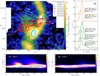 |
Fig. 12 Frame a: Integrated map of N2H+ (in K km s−1) of the junction region. The contours show the emission of 12CO (J = 1–0) at large velocities with respect to the bulk of the cloud. Each contour represent a different velocity as indicated in the inserted legend, and the corresponding levels in Tmb in order of increasing vlsr are 0.5, 1.0, 3.0, 3.0, 1.5, 1.1, 0.8 and 0.6 K. Frame b: Spectra of 12CO (J = 1–0) emission at different locations along the cuts, averaged over the Gaussian beams represented by the black circles in frame a, whose diameters show the beam FWHM (18′′). Frames c–d: Position-velocity diagrams of 12CO emission along the grey arrows shown in frame a, with offset increasing from east to west. The colour scales are cut to emphasise the fainter structures at large velocities. The contours show the emission of the central lines of N2 H + J = 1–0 (unresolved blend of F1F = 21–11, 23–12 and 22–11 lines) at Tmb = 0.15, 0.3, 0.5, 1.0 K. |
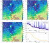 |
Fig. 13 Frames a–c: DSS2 blue map (λeff = 471 nm) of G202.3+2.5. The red contours show the 13CO emission from TRAO observations integrated between 6.3 and 9.3 km s−1
(frame a: with levels between |


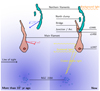 |
Fig. 14 Sketch of the proposed geometry of G202.3+2.5. The red structure corresponds to the main filament, the blue ones to the northern filaments. The front side of the main filament is illuminated by the cluster stars, and is responsible for most of the scattered light in the area 1 of Fig. 13. The northern filaments are in the shadow of material between them and the cluster, and are seen in extinction in front of background emission in the area 2 of Fig. 13. |
6.3 Investigating the scenario of triggered star formation
As mentioned in the previous section, if the collision hypothesis is correct, the most likely scenario is that a pre-existing relatively dense filament had its density increased in the process of the collision. We showed that an increase by a factor of three is realistic. Since the observed mass of the N2 H+ emitting gas is 141 M⊙ for a length of 6′ (1.3 pc), this structure has a linear mass of Mlin = 108 M⊙ pc−1. This is in the range of values (92–186 M⊙ pc−1) we found for the critical linear mass of gravitational instability under thermal and turbulent threshold in the junction region (Sect. 5.1.1). Considering that the N2H+ emitting mass is only a lower limit of the mass estimate, it suggests that the structure is gravitationally unstable, consistently with the fact that several protostars, including the most striking of the area (s1446), and several starless cores are detected in this structure. The masses of these protostellar sources reported by Montillaud et al. (2015) add up to 53.2 M⊙, implying a high star formation efficiency of ~20 or ~ 38% depending on which mass estimate is used for the N2H+ arc. In contrast, prior to the collision, the original filament would have contained three times less gas, that is M ~ 47 M⊙, its linear mass would have been Mlin ~ 36 M⊙ pc−1, a value slightly below the critical linear mass of 37–92 M⊙ pc−1 found in the northern filaments (Sect. 5.1.1), suggesting at best a moderate star formation activity, comparable to that observed in the north-western filament.
On the other hand, these masses include only the densest part of the junction region. The values in Table 2 with a column density threshold of 8 × 1021 cm−2 include larger areas with the envelope of intermediate densities. Assuming that the 210 M⊙ pc−1 reported for the junction region contains 108 M⊙ pc−1 of dense gas, if one divides only the mass of the dense layer by 3, the initial linear mass would have been 138 M⊙ pc−1, a value similar to the one estimated for the southern part of the main filament.
Altogether, it suggests that the initial filament was already forming stars and that the collision at least doubled its star formation activity. This situation is comparable to the one described by Dale et al. (2015), whose simulations demonstrate that triggering never consists in turning on star formation in an otherwise quiet cloud. Instead, it would imply the formation of stars that would not have formed without the triggering process, in a cloud which was already forming stars, so that both kinds of stars would be well mixed and extremely difficult to disentangle.
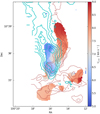 |
Fig. 15 Centroid map of the isolated hyperfine component of N2H+ in the junction region. The light blue and dark red lines show the contours of the 13CO emission from the IRAM data integrated between 3.6 and 6.0 km s−1, and between 6.3 and 9.3 km s−1, corresponding to the north-eastern filament and the main filament, respectively. The levels are between 3 and 18 K km s−1 by steps of 1.8 K km s−1, and between 12 and 18 K km s−1 by steps of 1.8 K km s−1 for the blue and red contours, respectively. In the white area, no line fitting was attempted because the N2 H + has a S/N <3. |
6.4 The role of the environment
The fact that the junction region is located at the edge of the Hα emission, a tracer of H II regions, suggests that the collision is related to the possible expansion of the H II region around NGC 2264. One possibility is that the main filament moves away from NGC 2264 as part of this expansion, and encountered the northern filaments. Alternatively, the northern filaments could be infalling towards NGC 2264, for example due to a global collapse of the whole region, hence colliding the shell around the H II region. It is therefore important to examine the age of the H II region to determine whether it is still expanding or has reached an equilibrium with the surrounding environment.
The only ionising star in NGC 2264 is S Mon, a multiple stellar system which includes a O7V star and a O9.5V star with a total mass of ~60 M⊙ (Gies et al. 1993; Cvetković et al. 2010). We did not find an age estimate of S Mon itself, but Sung & Bessel (2010) reports the age estimates of the pre-main sequence stars in the same substructure as S Mon. The first method, based on the SED fitting tool by Robitaille et al. (2006), leads to a median age of 1.5–2 Myr, with a dispersion between 0.2 and 3 Myr. The second method is based on isochrone fitting in colour-magnitude diagrams and leads to a median age of 3 Myr, with a dispersion between 1 and 6 Myr. Venuti et al. (2018) find similar results using Gaia-ESO data. As these authors, we assume S Mon’s age to be in the same range.
Williams et al. (2018) simulated the expansion of a spherical H II region into a uniform cold and neutral environment. According to their model, for the ionising luminosity of S Mon (logLEUV = 48.7 photons s−1, Venuti et al. 2018), the maximum over-shoot radius of the H II region is reached in ~15 Myr, and the equilibrium radius, slightly smaller than the maximum radius, is obtained after ~40 Myr. Hence, even with a conservative age estimate of 6 Myr, the H II region is likely to still be expanding. With a more realistic age of ~ 2−3 Myr, the ionising front and the shock fronts are still close to each other, with a radius of ~ 70% of the equilibrium radius. Williams et al. (2018) quote ~10 pc as a typical equilibrium radius, but there is a considerable scatter in this value (e.g. ~ 30 pc in λ Ori, Liu et al. 2016), and the complex geometry of the Hα emission indicates that the environment was not uniform when the H II region started its expansion. Therefore the distance of ~ 12 pc between S Mon and the edge of the Hα emission in the direction of the junction region seems a reasonable value for a still expanding H II region. We conclude that the shell is still expanding, and that this expansion is a possible candidate to explain the collision observed in the junction region.
On the other hand, it remains unclear whether the speed of the shock front can be sufficient to explain the gap in velocities between the main filament and the northern filaments. It can be seen in Figs. 11 and 15 that the difference in radial velocities is ~3−4 km s−1, so that the complete velocity difference can be even larger, especially if the line between S Mon and G202.3+2.5 is nearly perpendicular to the line of sight. In their Fig. 1, Williams et al. (2018) show a shock front with a velocity of only ~ 1 km s−1. Therefore it remains a possibility that, in addition to the expansion, the northern filaments have their own movement towards NGC 2264.
A first glimpse to this possibility is provided by observing the large-scale velocity gradients within the Mon OB 1 molecular complex. The 12CO (J = 1–0) data of the CfA 1.2 m telescope survey by Oliver et al. (1996) show a velocity gradient from the region of the S Mon sub-cluster (vlsr ≈ 10−12 km s−1) towards G202.3+2.5. A steeper gradient is also shown in the south of the S Mon sub-cluster towards the Cone nebula which has radial velocities comparable to those of G202.3+2.5 (vlsr ≈ 4−8 km s−1), but at a distance of only ~5 pc. Unfortunately the spatial and spectral resolution of these data are not sufficient to fully investigate the movement of the northern filaments with respect to NGC 2264. The 12CO (J = 3–2) data by Buckle et al. (2012), obtained with the JCMT telescope reveal a wealth of details at 14′′ resolution, but for an area limited to ~0.5° around S Mon.
7 Conclusion and perspectives
We have studied G202.3+2.5, a complex filamentary, star-forming cloud at the edge of the Monoceros OB 1 molecular complex, looking for a relationship between the dynamics of the filament and its star formation activity. We have examined its general density and thermal structure using dust emission maps from the Herschel Galactic cold cores programme, combined with TRAO 14-m and IRAM 30-m millimetre observations of mainly 12CO, 13CO, C18O, and N2 H+ (J = 1–0) molecular lines. From this data set, we also had characterised the compact sources in the first paper of this series and examined the variations of their properties with respect to the structure of the cloud. In addition here we characterised the dynamics of the cloud from the radial velocity field derived from the millimetre data. These analyses were combined to draw a multi-scale view of G202.3+2.5, from core scales (~ 0.1 pc) to the cloud scale (~10 pc), and led to propose a scenario of the recent star formation history of G202.3+2.5 in relation with its local environment in the Mon OB1 molecular complex.
The study has led to the following conclusions. G202.3+2.5 is found to be actively forming stars, and the filaments’ linear masses suggest that this activity will be sustained in the near future.
IRAM 12CO observations confirm a known outflow from the brightest and massive (Mdust ≈ 22 M⊙) protostellar source in G202.3+2.5, and suggest that this source could also be responsible for a second outflow in a different direction. The structure of the main outflow suggests that it was emitted in an intermittent fashion, and we estimated the oldest outburst, responsible for a large Herbig–Haro object, to be ~ 2 × 10⁴ yr old.
The structure derived solely from dust observations is very misleading. The north-western filament, which looks like a single structure in Herschel maps, appears in IRAM data as the superposition of two independent velocity components. In dust maps, the junction region seems to be the point where the main filament forks into two secondary filaments (the northern filaments), whereas TRAO 13CO observations show that the two northern filaments are two parts of the same structure at vlsr ~ 4 km s−1, while the main filament is a different structure at vlsr ~ 7−8 km s−1.
The velocity components identified from the IRAM 13CO data show that the two main velocity structures, namely the main filament and the northern filaments, merge in velocity in the junction region where the densest gas is found and traced by N2 H+. The N2 H+ emission exhibits a large velocity gradient, emitting continuously from the velocity of one structure to the other, suggesting that the dense gas is a compressed layer between the two structures.
The qualitative analysis of the extinction and scattered light in the visible DSS surface brightness map of the cloud led to the conclusion that the northern filaments are behind the main filament. Thus the shift in radial velocities implies that the two structures are moving towards each other, supporting the idea of a collision between them in the junction region.
Based on the typical chemical age of N2H+ in dense cores, we proposed a scenario in which the junction region would be the result of a collision that started ~ 105 yr ago between the main filament and the southern tip of the northern filaments. We showed that in the frame of this scenario, our data are compatible with the idea that the colliding part of the main filament was already relatively dense and forming stars, similarly to the rest of this filament, and accreted additional gas from the northern filaments at a rate Ṁ ~ 1 × 10⁻³ M⊙ yr−1.
We interpreted the local peak in star formation activity in the junction region, and more specifically in the N2 H+ emitting gas, as the result of the increase in gas density, itself resulting from the collision. Therefore this region falls under the frame of triggered star formation in the sense of Type I triggering defined by Dale et al. (2015): “A temporary or long-term increase in the star formation rate”.
The collision scenario was put in perspective with the local environment of G202.3+2.5. The cloud is at the edge of the H II region around the nearby open cluster NGC 2264 and its most massive member, the O-type binary S Mon. We showed that this H II region is young enough to still be expanding, and is therefore a candidate for the origin of the collision. However, we cannot rule out the idea that the northern filaments move towards NGC 2264 as part of a possible global collapse of the region, contributingor even possibly dominating the collision velocity.
The Monoceros OB 1 molecular cloud appears as a good target to characterise the global evolution of a giant molecular cloud. Additional steps are already engaged to complement the multiscale approach of this study.
The large scale 12CO and 13CO (1–0) emissions in the Monoceros OB 1 molecular cloud will be observed to further study the connection between G202.3+2.5 and NGC 2264 and test the ideas of global or hierarchical collapse of this region.
The collision in the junction region needs to be further characterised. Shock tracers, such as SiO(2–1) (Jiménez-Serra et al. 2010) or H2S and SO2 transitions (Codella et al. 2003), will be observed to constrain the collision velocity and morphology. In addition, we will look for infall signatures in the junction region, by searching asymmetry in high-spectral resolution observations of HCO+(1–0) in combination with the N2H+(1–0) line to tracethe systemic velocity (Fuller et al. 2005).
Finally, the magnetic field geometry and strength, ideally measured at angular resolutions comparable to that of the molecular line tracers discussed here, are key to understand the present state and the history of Mon OB 1. We have measured dust polarized emission at 850 μm with the polarimetre POL-2 at the JCMT 15-m telescope (Liu, et al., in prep.). Such observations have proven to be good tracers of the plane-of-sky projected B-field morphologies from large to small scales (e.g. Matthews et al. 2009; Dotson et al. 2010; Hull et al. 2014; Zhang et al. 2014; Cortes et al. 2016; Koch et al. 2018; Liu et al. 2018c,b). Given the high densities in the junction regions, the B-field morphology here could reveal dragged-in and pinched B-fields as it is observed in gravity-dominated and collapsing cores (e.g., Girart et al. 2009; Tang et al. 2009). In combination with molecular line tracers, correlations between velocity gradients and B-field orientation can be searched to constrain the role of the B-field in the accretion process, and the magnetic support can be evaluated to firmly conclude on core and filament stability.
Acknowledgements
This work is based on observations carried out under project number 113-16 with the IRAM 30-m telescope. IRAM is supported by INSU/CNRS (France), MPG (Germany) and IGN (Spain). J.M. warmly thanks the staff of the 30-m for its kind and efficient help, and in particular Pablo Garcia for stimulating discussions. The project leading to this publication has received funding from the “Soutien à la recherche de l’observatoire” by the OSU THETA. This work was supported by the Programme National “Physique et Chimie du Milieu Interstellaire” (PCMI) of CNRS/INSU with INC/INP co-funded by CEA and CNES. J.M., R.B., D.C., and V.L.T. thank the French ministry of foreign affairs (French embassy in Budapest) and the Hungarian national office for research and innovation (NKFIH) for financial support (Balaton program 40470VL/ 2017-2.2.5-TéT-FR-2017-00027). The project leading to this publication has received funding from the European Union’s Horizon 2020 research and innovation programme under grant agreement No 730 562 [RadioNet]. This research used data from the Second Palomar Observatory Sky Survey (POSS-II), which was made by the California Institute of Technology with funds from the National Science Foundation, the National Geographic Society, the Sloan Foundation, the Samuel Oschin Foundation, and the Eastman Kodak Corporation. M.J. and E.R.M. acknowledge the support of the Academy of Finland Grant No. 285769. This research has made use of the SVO Filter Profile Service (http://svo2.cab.inta-csic.es/theory/fps/) supported from the Spanish MINECO through grant AyA2014-55216. J.H.He is supported by the NSF of China under Grant Nos. 11873086 and U1631237, partly by Yunnan province (2017HC018), and also partly by the Chinese Academy of Sciences (CAS) through a grant to the CAS South America Center for Astronomy (CASSACA) in Santiago, Chile. C.W.L. was supported by the Basic Science Research Program through the National Research Foundation of Korea (NRF) funded by the Ministry of Education, Science and Technology (NRF-2019R1A2C1010851). S.Z. acknowledges the support of NAOJ ALMA Scientific Research Grant Number 2016-03B. K.W. acknowledges support by the National Key Research and Development Program of China (2017YFA0402702), the National Science Foundation of China (11973013, 11721303), and the starting grant at the Kavli Institute for Astronomy and Astrophysics, Peking University (7101502016). DA acknowledges the funding from Ministry of Education and Science of the Republic of Kazakhstan state-targeted programme BR05236454. DA acknowledges the funding from Nazarbayev University FCDRG110119FD4503 grant support.
Appendix A Integrated intensity and channel maps
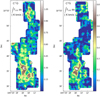 |
Fig. A.1 Integrated intensity maps of C17O (left) and C34S (right). The maps are smoothed with a Gaussian kernel of FWHM = 25′′. |
Appendix B Linear mass formula for turbulent support
The critical linear mass of an isothermal, thermally and turbulence-supported cylinder is a usual quantity to characterise the stability of a self-gravitating interstellar filament. However, several versions of the formula are used in the literature that are mutually incompatible (e.g. Liu et al. 2018c; Pattle et al. 2017), based on different recipes to convert between 1D and 3D velocity dispersions. We propose here a simple justification of the formulae used in Sect. 5.1.1, based on the pioneering works by Chandrasekhar (1951) and Ostriker (1964). Ostriker (1964) demonstrated that the critical linear mass of a thermally supported isothermal infinite cylinder is:
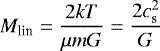 (B.1)
(B.1)
where T is the filament temperature, m is the mass of the hydrogen nucleus, μm is the mean particle mass, and  is the so-called isothermal sound speed. We note that this quantity differs from the actual sound speed by the adiabatic factor γ, and corresponds to the 1D rms of particle thermal velocity.
Chandrasekhar (1951) showed in the case of isotropic microturbulence in a uniform medium that the equations by Jeans are modified by the transformation  , where U is the 3D rms turbulent velocity. We note that the factor 1∕3 makes the term 1∕3U2 correspond to the square of the 1D rms turbulent velocity.
In Chandrasekhar’s work, cs is the actual (adiabatic) sound speed, but the transformation can still be applied to Ostriker’s formula since not only the difference with the isothermal sound speed is negligible compared to the uncertainties in our study, but also Chandrasekhar’s assumption of an adiabatic evolution of the gas is independent of the reasoning leading to the transformation.
From the observational point of view, the measured velocity dispersions are intrinsically 1D, along the line-of-sight. The thermal velocity line width corresponds to the isothermal sound speed, and we assume that the H2 non-thermal velocity dispersion σNT is entirely caused by the isotropic turbulence and therefore corresponds to the term (1∕3)U2 in Chandrasekhar’s equations. As a result, the critical linear mass has the form:
 (B.2)
(B.2)
where cs can be estimated, for example, from dust temperature or from ammonia observations (Wilson & Rood 1994), and σNT can be derived from the gas temperature and the linewidth of a molecular tracer, for example 13CO (1–0) as in Sect. 5.1.1.
Finally, we note that it physically makes sense that only the 1D rms velocity dispersions appear in this equation. In the law of ideal gas, the thermal gas pressure is  , where cs is the 1D rms of particle thermal velocity. Similarly, the turbulent pressure is usually defined as
  , where σNT is also the 1D rms velocity (McKee & Ostriker 2007, between their Eqs. (8) and (9)). Since Eq. (B.1) is equivalent to Mlin = 2Pth∕ρG, it makes sense that the generalisation to turbulent support is Mlin = 2(Pth + Pturb)∕ρG, which is equivalent to Eq. (B.2).
 |
Fig. A.2 Channel maps of C18O (top), C17O (second row), CS (third row), C34S (forth row) and N2H+ (bottom). The maps of C18O and N2 H+ are smoothed with a Gaussian kernel of FWHM = 5′′, and C17O and C34S with FWHM = 25′′. For N2 H+, the hyperfine components were fitted assuming the LTE line ratios, and only the isolated component is shown here. For C17O, the target line (F = 3/2–5/2) is blended with the F = 7/2–5/2 component, but the F = 5/2–5/2 one is visible, shifted by vlsr = − 3.3 km s−1. |
References
- Allen, D. A. 1972, ApJ, 172, L55 [NASA ADS] [CrossRef] [Google Scholar]
- Anderson, L. D., Bania, T. M., Balser, D. S., et al. 2014, ApJS, 212, 1 [NASA ADS] [CrossRef] [Google Scholar]
- André, P., Men’shchikov, A., Bontemps, S., et al. 2010, A&A, 518, L102 [NASA ADS] [CrossRef] [EDP Sciences] [Google Scholar]
- Beckwith, S. V. W., Sargent, A. I., Chini, R. S., & Guesten, R. 1990, AJ, 99, 924 [NASA ADS] [CrossRef] [Google Scholar]
- Buckle, J. V., Richer, J. S., & Davis, C. J. 2012, MNRAS, 423, 1127 [NASA ADS] [CrossRef] [Google Scholar]
- Chandrasekhar, S. 1951, Phil. Trans. R. Soc. London, Ser. A, 210, 18 [NASA ADS] [CrossRef] [MathSciNet] [Google Scholar]
- Codella, C., Bachiller, R., Benedettini, M., & Caselli, P. 2003, MNRAS, 341, 707 [NASA ADS] [CrossRef] [Google Scholar]
- Cortes, P. C., Girart, J. M., Hull, C. L. H., et al. 2016, ApJ, 825, L15 [NASA ADS] [CrossRef] [Google Scholar]
- Csengeri, T., Bontemps, S., Schneider, N., Motte, F., & Dib, S. 2011, A&A, 527, A135 [NASA ADS] [CrossRef] [EDP Sciences] [Google Scholar]
- Csengeri, T., Weiss, A., Wyrowski, F., et al. 2016, A&A, 585, A104 [NASA ADS] [CrossRef] [EDP Sciences] [Google Scholar]
- Cutri, R. M., Wright, E. L., Conrow, T., et al. 2011, Explanatory Supplement to the WISE Preliminary Data Release Products, Tech. rep [Google Scholar]
- Cvetković, Z., Vince, I., & Ninković, S. 2010, New Astron., 15, 302 [NASA ADS] [CrossRef] [Google Scholar]
- Dahm, S. E. 2008, in Handbook of Star Forming Regions (San Francisco: ASP Monograph Publications), I, 966 [Google Scholar]
- Dahm, S. E., & Simon, T. 2005, AJ, 129, 829 [NASA ADS] [CrossRef] [Google Scholar]
- Dale, J. E., Haworth, T. J., & Bressert, E. 2015, MNRAS, 450, 1199 [NASA ADS] [CrossRef] [Google Scholar]
- Dotson, J. L., Vaillancourt, J. E., Kirby, L., et al. 2010, ApJS, 186, 406 [NASA ADS] [CrossRef] [Google Scholar]
- Eden, D. J., Liu, T., Kim, K.-T., et al. 2019, MNRAS, 485, 2895 [NASA ADS] [CrossRef] [Google Scholar]
- Endres, C. P., Schlemmer, S., Schilke, P., Stutzki, J., & Müller, H. S. P. 2016, J. Mol. Spectr., 327, 95 [NASA ADS] [CrossRef] [Google Scholar]
- Enoch, M. L., Glenn, J., Evans, II, N. J., et al. 2007, ApJ, 666, 982 [NASA ADS] [CrossRef] [Google Scholar]
- Finkbeiner, D. P. 2003, ApJS, 146, 407 [NASA ADS] [CrossRef] [Google Scholar]
- Fuller, G. A., Williams, S. J., & Sridharan, T. K. 2005, A&A, 442, 949 [NASA ADS] [CrossRef] [EDP Sciences] [Google Scholar]
- Gies, D. R., Mason, B. D., Hartkopf, W. I., et al. 1993, AJ, 106, 2072 [NASA ADS] [CrossRef] [Google Scholar]
- Girart, J. M., Beltrán, M. T., Zhang, Q., Rao, R., & Estalella, R. 2009, Science, 324, 1408 [NASA ADS] [CrossRef] [PubMed] [Google Scholar]
- Griffin, M. J., Abergel, A., Abreu, A., et al. 2010, A&A, 518, L3 [Google Scholar]
- Hacar, A., Tafalla, M., Kauffmann, J., & Kovács, A. 2013, A&A, 554, A55 [NASA ADS] [CrossRef] [EDP Sciences] [Google Scholar]
- Hacar, A., Kainulainen, J., Tafalla, M., Beuther, H., & Alves, J. 2016, A&A, 587, A97 [NASA ADS] [CrossRef] [EDP Sciences] [Google Scholar]
- Hacar, A., Tafalla, M., & Alves, J. 2017, A&A, 606, A123 [NASA ADS] [CrossRef] [EDP Sciences] [Google Scholar]
- Hacar, A., Tafalla, M., Forbrich, J., et al. 2018, A&A, 610, A77 [NASA ADS] [CrossRef] [EDP Sciences] [Google Scholar]
- Henshaw, J. D., Jiménez-Serra, I., Longmore, S. N., et al. 2017, MNRAS, 464, L31 [NASA ADS] [CrossRef] [Google Scholar]
- Hull, C. L. H., Plambeck, R. L., Kwon, W., et al. 2014, ApJS, 213, 13 [NASA ADS] [CrossRef] [Google Scholar]
- Jiménez-Serra, I., Caselli, P., Tan, J. C., et al. 2010, MNRAS, 406, 187 [NASA ADS] [CrossRef] [Google Scholar]
- Juvela, M., Ristorcelli, I., Montier, L. A., et al. 2010, A&A, 518, L93 [NASA ADS] [CrossRef] [EDP Sciences] [Google Scholar]
- Juvela, M., Ristorcelli, I., Pagani, L., et al. 2012, A&A, 541, A12 [NASA ADS] [CrossRef] [EDP Sciences] [Google Scholar]
- Juvela, M., Montillaud, J., Ysard, N., & Lunttila, T. 2013, A&A, 556, A63 [NASA ADS] [CrossRef] [EDP Sciences] [Google Scholar]
- Koch, P. M., Tang, Y.-W., Ho, P. T. P., et al. 2018, ApJ, 855, 39 [NASA ADS] [CrossRef] [Google Scholar]
- Lippok, N., Launhardt, R., Semenov, D., et al. 2013, A&A, 560, A41 [NASA ADS] [CrossRef] [EDP Sciences] [Google Scholar]
- Liu, T., Zhang, Q., Kim, K.-T., et al. 2016, ApJS, 222, 7 [NASA ADS] [CrossRef] [Google Scholar]
- Liu, T., Kim, K.-T., Juvela, M., et al. 2018a, ApJS, 234, 28 [NASA ADS] [CrossRef] [Google Scholar]
- Liu, T., Kim, K.-T., Liu, S.-Y., et al. 2018b, ApJ, 869, L5 [NASA ADS] [CrossRef] [Google Scholar]
- Liu, T., Li, P. S., Juvela, M., et al. 2018c, ApJ, 859, 151 [NASA ADS] [CrossRef] [Google Scholar]
- López-Sepulcre, A., Cesaroni, R., & Walmsley, C. M. 2010, A&A, 517, A66 [NASA ADS] [CrossRef] [EDP Sciences] [Google Scholar]
- Malinen, J., Juvela, M., Collins, D. C., Lunttila, T., & Padoan, P. 2011, A&A, 530, A17 [CrossRef] [EDP Sciences] [Google Scholar]
- Margulis, M., Lada, C. J., & Snell, R. L. 1988, ApJ, 333, 316 [NASA ADS] [CrossRef] [Google Scholar]
- Matthews, B. C., McPhee, C. A., Fissel, L. M., & Curran, R. L. 2009, ApJS, 182, 143 [NASA ADS] [CrossRef] [Google Scholar]
- McKee, C. F. 1989, ApJ, 345, 782 [NASA ADS] [CrossRef] [Google Scholar]
- McKee, C. F., & Ostriker, E. C. 2007, ARA&A, 45, 565 [NASA ADS] [CrossRef] [Google Scholar]
- McLean, B. J., Greene, G. R., Lattanzi, M. G., & Pirenne, B. 2000, ASP Conf. Ser., 216, 145 [NASA ADS] [Google Scholar]
- Meisner, A. M., & Finkbeiner, D. P. 2014, ApJ, 781, 5 [NASA ADS] [CrossRef] [Google Scholar]
- Montier, L. A., Pelkonen, V.-M., Juvela, M., Ristorcelli, I., & Marshall, D. J. 2010, A&A, 522, A83 [NASA ADS] [CrossRef] [EDP Sciences] [Google Scholar]
- Montillaud, J., Juvela, M., Rivera-Ingraham, A., et al. 2015, A&A, 584, A92 [NASA ADS] [CrossRef] [EDP Sciences] [Google Scholar]
- Montillaud, J., Juvela, M., Vastel, C., et al. 2019, A&A, 631, L1 [CrossRef] [EDP Sciences] [Google Scholar]
- Motte, F., Bontemps, S., & Louvet, F. 2018, ARA&A, 56, 41 [NASA ADS] [CrossRef] [Google Scholar]
- Nakamura, F., Sugitani, K., Tanaka, T., et al. 2014, ApJ, 791, L23 [NASA ADS] [CrossRef] [Google Scholar]
- Nakamura, F., Dobashi, K., Shimoikura, T., Tanaka, T., & Onishi, T. 2017, ApJ, 837, 154 [NASA ADS] [CrossRef] [Google Scholar]
- Ogura, K. 1995, ApJ, 450, L23 [NASA ADS] [CrossRef] [Google Scholar]
- Oliver, R. J., Masheder, M. R. W., & Thaddeus, P. 1996, A&A, 315, 578 [NASA ADS] [Google Scholar]
- Ostriker, J. 1964, ApJ, 140, 1056 [NASA ADS] [CrossRef] [MathSciNet] [Google Scholar]
- Padoan, P., Haugbølle, T., Nordlund, A., & Frimann, S. 2017, ApJ, 840, 48 [NASA ADS] [CrossRef] [Google Scholar]
- Pagani, L., Daniel, F., & Dubernet, M.-L. 2009, A&A, 494, A719 [NASA ADS] [CrossRef] [EDP Sciences] [Google Scholar]
- Pattle, K., Ward-Thompson, D., Berry, D., et al. 2017, ApJ, 846, 122 [NASA ADS] [CrossRef] [Google Scholar]
- Peretto, N., André, P., & Belloche, A. 2006, A&A, 445, 979 [NASA ADS] [CrossRef] [EDP Sciences] [Google Scholar]
- Peretto, N., Fuller, G. A., André, P., et al. 2014, A&A, 561, A83 [NASA ADS] [CrossRef] [EDP Sciences] [Google Scholar]
- Pety, J., Guzmán, V. V., Orkisz, J. H., et al. 2017, A&A, 599, A98 [NASA ADS] [CrossRef] [EDP Sciences] [Google Scholar]
- Pilleri, P., Montillaud, J., Berné, O., & Joblin, C. 2012, A&A, 542, A69 [NASA ADS] [CrossRef] [EDP Sciences] [Google Scholar]
- Pineda, J. L., Goldsmith, P. F., Chapman, N., et al. 2010, ApJ, 721, 686 [NASA ADS] [CrossRef] [Google Scholar]
- Planck Collaboration XXIII. 2011, A&A, 536, A23 [NASA ADS] [CrossRef] [EDP Sciences] [Google Scholar]
- Planck Collaboration, XXVIII. 2016, A&A, 594, A28 [NASA ADS] [CrossRef] [EDP Sciences] [Google Scholar]
- Poglitsch, A., Waelkens, C., Geis, N., et al. 2010, A&A, 518, L2 [NASA ADS] [CrossRef] [EDP Sciences] [Google Scholar]
- Rapson, V. A., Pipher, J. L., Gutermuth, R. A., et al. 2014, ApJ, 794, 124 [NASA ADS] [CrossRef] [EDP Sciences] [Google Scholar]
- Reipurth, B., & Bally, J. 2001, ARA&A, 39, 403 [NASA ADS] [CrossRef] [Google Scholar]
- Reipurth, B., Bally, J., & Devine, D. 1997, AJ, 114, 2708 [NASA ADS] [CrossRef] [Google Scholar]
- Reipurth, B., Pettersson, B., Armond, T., Bally, J., & Vaz, L. P. R. 2004a, AJ, 127, 1117 [NASA ADS] [CrossRef] [Google Scholar]
- Reipurth, B., Yu, K. C., Moriarty-Schieven, G., et al. 2004b, AJ, 127, 1069 [NASA ADS] [CrossRef] [Google Scholar]
- Renaud, F., Bournaud, F., Emsellem, E., et al. 2013, MNRAS, 436, 1836 [NASA ADS] [CrossRef] [Google Scholar]
- Rivera-Ingraham, A., Ristorcelli, I., Juvela, M., et al. 2017, A&A, 601, A94 [NASA ADS] [CrossRef] [EDP Sciences] [Google Scholar]
- Robitaille, T. P., Whitney, B. A., Indebetouw, R., Wood, K., & Denzmore, P. 2006, ApJS, 167, 256 [NASA ADS] [CrossRef] [Google Scholar]
- Sargent, A. I., van Duinen, R. J., Nordh, H. L., et al. 1984, A&A, 135, 377 [NASA ADS] [Google Scholar]
- Schneider, N., Csengeri, T., Bontemps, S., et al. 2010, A&A, 520, A1 [NASA ADS] [CrossRef] [EDP Sciences] [Google Scholar]
- Schreyer, K., Helmich, F. P., van Dishoeck, E. F., & Henning, T. 1997, A&A, 326, 347 [NASA ADS] [Google Scholar]
- Shetty, R., Kauffmann, J., Schnee, S., & Goodman, A. A. 2009a, ApJ, 696, 676 [NASA ADS] [CrossRef] [Google Scholar]
- Shetty, R., Kauffmann, J., Schnee, S., Goodman, A. A., & Ercolano, B. 2009b, ApJ, 696, 2234 [NASA ADS] [CrossRef] [Google Scholar]
- Smith, R. J., Glover, S. C. O., Klessen, R. S., & Fuller, G. A. 2016, MNRAS, 455, 3640 [NASA ADS] [CrossRef] [Google Scholar]
- Sun, J., Leroy, A. K., Schruba, A., et al. 2018, ApJ, 860, 172 [NASA ADS] [CrossRef] [Google Scholar]
- Sung, H., & Bessel, M. S. 2010, AJ, 140, 2070 [NASA ADS] [CrossRef] [Google Scholar]
- Tang, Y.-W., Ho, P. T. P., Girart, J. M., et al. 2009, ApJ, 695, 1399 [NASA ADS] [CrossRef] [Google Scholar]
- Tauber, J. A., Mandolesi, N., Puget, J.-L., et al. 2010, A&A, 520, A1 [NASA ADS] [CrossRef] [EDP Sciences] [Google Scholar]
- Traficante, A., Fuller, G. A., Billot, N., et al. 2017, MNRAS, 470, 3882 [NASA ADS] [CrossRef] [Google Scholar]
- Traficante, A., Duarte-Cabral, A., Elia, D., et al. 2018a, MNRAS, 477, 2220 [NASA ADS] [CrossRef] [Google Scholar]
- Traficante, A., Fuller, G. A., Smith, R. J., et al. 2018b, MNRAS, 473, 4975 [NASA ADS] [CrossRef] [Google Scholar]
- Vázquez-Semadeni, E., Gómez, G. C., Jappsen, A.-K., Ballesteros-Paredes, J., & Klessen, R. S. 2009, ApJ, 707, 1023 [NASA ADS] [CrossRef] [Google Scholar]
- Vázquez-Semadeni, E., Palau, A., Ballesteros-Paredes, J., Gómez, G. C., & Zamora-Avilés, M. 2019, MNRAS, submitted [arXiv:1903.11247] [Google Scholar]
- Venuti, L., Prisinzano, L., Sacco, G. G., et al. 2018, A&A, 609, A10 [NASA ADS] [CrossRef] [EDP Sciences] [Google Scholar]
- Wang, K., Zahorecz, S., Cunningham, M. R., et al. 2018, Res. Notes Amer. Astron. Soc., 2, 2 [NASA ADS] [CrossRef] [Google Scholar]
- Williams, J. P., & Garland, C. A. 2002, ApJ, 568, 259 [NASA ADS] [CrossRef] [Google Scholar]
- Williams, R. J. R., Bisbas, T. G., Haworth, T. J., & Mackey, J. 2018, MNRAS, 479, 2016 [NASA ADS] [CrossRef] [Google Scholar]
- Wilson, T. L.,& Rood, R. 1994, ARA&A, 32, 191 [NASA ADS] [CrossRef] [Google Scholar]
- Wilson, T. L., Rohlfs, K., & Hüttemeister, S. 2013, Tools of Radio Astronomy (Berlin: Springer Science & Business Media) [CrossRef] [Google Scholar]
- Wolf-Chase, G., Moriarty-Schieven, G., Fich, M., & Barsony, M. 2003, MNRAS, 344, 809 [NASA ADS] [CrossRef] [Google Scholar]
- Wright, E. L., Eisenhardt, P. R. M., Mainzer, A. K., et al. 2010, AJ, 140, 1868 [Google Scholar]
- Wyrowski, F., Güsten, R., Menten, K. M., et al. 2016, A&A, 585, A149 [NASA ADS] [CrossRef] [EDP Sciences] [Google Scholar]
- Yamamoto, S. 2017, Introduction to Astrochemistry: Chemical Evolution from Interstellar Clouds to Star and Planet Formation (Berlin: Springer) [Google Scholar]
- Zhang, Q., Qiu, K., Girart, J. M., et al. 2014, ApJ, 792, 116 [NASA ADS] [CrossRef] [Google Scholar]
SPIRE observer’s manual, http://herschel.esac.esa.int/Documentation.shtml
To limit the noise in the map, only data cube cells with Tmb greater than 1.5 and 0.1 K in 13CO and C18O, respectively, were included. Using lower thresholds makes the map noisier, but does not change the average values nor the morphology significantly.
All Tables
Approximate lengths and masses of the main structures identified in the column density map.
Properties of the five largest 13CO velocity-coherent structures identified in G202.3+2.5.
All Figures
|
Fig. 1 Three-colour composite image of Monoceros OB1 molecular complex. Red: Planck 857 GHz; green: WISE 12 μm from Meisner & Finkbeiner (2014); blue: Hα. The white and yellow contours are the footprints of Herschel SPIRE, IRAM, and TRAO observations, as labelled. |
| In the text | |
|
Fig. 2 Left: column density of molecular hydrogen in G202.3+2.5 as derived from SPIRE bands, assuming a modified black-body SED with fixed β = 2. Right: dust temperature in G202.3+2.5 derived from the same SED fitting. In both frames, the dark-blue solid line shows the footprint of our IRAM OTF observations, and the ellipses show the location, size (full-width at half-maximum of a Gaussian fit) and orientation of the submillimetre compact sources extracted by Montillaud et al. (2015). The regions defined in the main text are indicated with white shapes. In both frames, the inset shows a zoom to the junction region (white rectangle). |
| In the text | |
|
Fig. 3 Integrated intensity maps of the main detected lines in our IRAM observations. The sources s1454 (North clump) and s1446 (NGC 2264 H) are indicated in each frame. A scale bar is shown in frame a. The ellipses in frame b show the GCC sources with the same colour code as in Fig. 2: red for protostellar, blue for starless, and black for undetermined. The black and red squares in frame c show the areas where the average spectra in Fig. 5 were computed. The structures named “the arc” and “the bar” are shown in frame e. |
| In the text | |
|
Fig. 4 Integrated intensity map of 13CO in our TRAO observations. The black line shows the footprint of the IRAM observations. A scale bar is shown in the top left corner. |
| In the text | |
|
Fig. 5 Spectra of CO isotopologues in the north clump (black) and in the main filament (red). Spectra are averaged within 2 arcmin-wide square regions centred at (α, δ) = (6:40:54.9;+10:55:40.8) for the north clump and (α, δ) = (6:41:03.6;+10:34:28.7) for the main filament. In the C17O (J = 1–0) transition, the three vertical blue lines indicate the positions of the three hyperfine components assuming vlsr = 5.3 km s−1. |
| In the text | |
|
Fig. 6 Column density maps of 13CO (frame a) and C18O (frame b), and their ratio (frame c) normalised to the expected 13CO/C18O from Wilson & Rood (1994). Frame d: Excitation temperature of 12CO.
Frame e: Integrated |
| In the text | |
|
Fig. 7 Left: velocity integrated map of 13CO in K km s−1. Right: position-velocity diagram along the dashed line of the left frame. The two circles on the map in the left frame show the locations of the spectra shown in Fig. 8. |
| In the text | |
|
Fig. 8 Spectra of CO, 13CO and C18O (J = 1–0) in the junction (left) and bridge (right) regions at the locations marked by black circles in Fig. 7. The spectra of CO is divided by 2. The black dashed lines are the 3-component Gaussian fit of the 13CO lines (Sect. 4.2.1). |
| In the text | |
|
Fig. 9 Top: 13CO channel maps from TRAO data. Middle: 13CO channel maps from IRAM data. Bottom: 12CO channel maps from IRAM data. The channel velocities are written in the top corners. In the two first and last frames, the sources from the GCC catalogue are shown as white ellipses and the arc and bar regions are shown as white lines. The north clump and NGC 2264 H are labelled as “s1454” and “s1446” in TRAO maps, and “N” and “H” in IRAM maps, respectively.Scale bars are in the next to last frames. |
| In the text | |
|
Fig. 10 Distribution of line centroids in the position-position-velocity space for 13CO (left) and C18O (right). The colours vary with velocity to help the 3D visualisation. The black points are projections of the colour ones on the faces of the box. In the right frame, lines joining the projections to the colour points are drawn to help visualising in 3D the positions of s1454 (in the north clump), s1461 (at the root of the north-eastern filament), s1446 (in the arc), and s1453 (just north to the arc). |
| In the text | |
|
Fig. 11 Frame a: 3D position-position-velocity view of the velocity-coherent structures in 13CO. The pale colours are projections of the structures onto the plane of the sky, the α − v plane and the δ − v plane. Each colour corresponds to a different structure. The id numbers of the five components tabulated in Table 3 are indicated in the δ − v plane. Frame b: Thermal emission of dust in G202.3+2.5 at 250 μm (Herschel/SPIRE). Coloured regions show the same velocity-coherent structures as in frame a for 13CO J = 1–0 (no symbol) and N2H+ J = 1–0 (isolated component, with hatches). The colour scale shows the average radial velocity of each structure. Transparency reveals the overlaps between the structures. Sources 1446, 1449, 1454, and 1457 are indicated in black. The white lines show the arc and the bar. The coloured numbers indicate the five main VCSs. |
| In the text | |
|
Fig. 12 Frame a: Integrated map of N2H+ (in K km s−1) of the junction region. The contours show the emission of 12CO (J = 1–0) at large velocities with respect to the bulk of the cloud. Each contour represent a different velocity as indicated in the inserted legend, and the corresponding levels in Tmb in order of increasing vlsr are 0.5, 1.0, 3.0, 3.0, 1.5, 1.1, 0.8 and 0.6 K. Frame b: Spectra of 12CO (J = 1–0) emission at different locations along the cuts, averaged over the Gaussian beams represented by the black circles in frame a, whose diameters show the beam FWHM (18′′). Frames c–d: Position-velocity diagrams of 12CO emission along the grey arrows shown in frame a, with offset increasing from east to west. The colour scales are cut to emphasise the fainter structures at large velocities. The contours show the emission of the central lines of N2 H + J = 1–0 (unresolved blend of F1F = 21–11, 23–12 and 22–11 lines) at Tmb = 0.15, 0.3, 0.5, 1.0 K. |
| In the text | |
|
Fig. 13 Frames a–c: DSS2 blue map (λeff = 471 nm) of G202.3+2.5. The red contours show the 13CO emission from TRAO observations integrated between 6.3 and 9.3 km s−1
(frame a: with levels between |
| In the text | |
|
Fig. 14 Sketch of the proposed geometry of G202.3+2.5. The red structure corresponds to the main filament, the blue ones to the northern filaments. The front side of the main filament is illuminated by the cluster stars, and is responsible for most of the scattered light in the area 1 of Fig. 13. The northern filaments are in the shadow of material between them and the cluster, and are seen in extinction in front of background emission in the area 2 of Fig. 13. |
| In the text | |
|
Fig. 15 Centroid map of the isolated hyperfine component of N2H+ in the junction region. The light blue and dark red lines show the contours of the 13CO emission from the IRAM data integrated between 3.6 and 6.0 km s−1, and between 6.3 and 9.3 km s−1, corresponding to the north-eastern filament and the main filament, respectively. The levels are between 3 and 18 K km s−1 by steps of 1.8 K km s−1, and between 12 and 18 K km s−1 by steps of 1.8 K km s−1 for the blue and red contours, respectively. In the white area, no line fitting was attempted because the N2 H + has a S/N <3. |
| In the text | |
|
Fig. A.1 Integrated intensity maps of C17O (left) and C34S (right). The maps are smoothed with a Gaussian kernel of FWHM = 25′′. |
| In the text | |
|
Fig. A.2 Channel maps of C18O (top), C17O (second row), CS (third row), C34S (forth row) and N2H+ (bottom). The maps of C18O and N2 H+ are smoothed with a Gaussian kernel of FWHM = 5′′, and C17O and C34S with FWHM = 25′′. For N2 H+, the hyperfine components were fitted assuming the LTE line ratios, and only the isolated component is shown here. For C17O, the target line (F = 3/2–5/2) is blended with the F = 7/2–5/2 component, but the F = 5/2–5/2 one is visible, shifted by vlsr = − 3.3 km s−1. |
| In the text | |
Current usage metrics show cumulative count of Article Views (full-text article views including HTML views, PDF and ePub downloads, according to the available data) and Abstracts Views on Vision4Press platform.
Data correspond to usage on the plateform after 2015. The current usage metrics is available 48-96 hours after online publication and is updated daily on week days.
Initial download of the metrics may take a while.