| Issue |
A&A
Volume 694, February 2025
|
|
|---|---|---|
| Article Number | A199 | |
| Number of page(s) | 20 | |
| Section | Interstellar and circumstellar matter | |
| DOI | https://doi.org/10.1051/0004-6361/202348883 | |
| Published online | 13 February 2025 | |
Multi-scale analysis of the Monoceros OB 1 star-forming region
III. Tracing the dense gas in the massive clump G202.3+2.5
1
Eötvös Loránd University, Department of Astronomy,
Pázmány Péter sétány 1/A,
1117
Budapest,
Hungary
2
Institut UTINAM, CNRS UMR 6213, OSU THETA, Université de Franche-Comté,
41 bis avenue de l’Observatoire,
25000
Besançon,
France
3
IRAP, Université de Toulouse, CNRS, CNES, UPS,
9 av. du Colonel Roche, BP 44346,
31028
Toulouse,
France
4
Department of Physics,
PO Box 64,
00014 University of Helsinki,
Finland
5
University of Debrecen, Faculty of Science and Technology,
Egyetem tér 1,
4032
Debrecen,
Hungary
★ Corresponding author; This email address is being protected from spambots. You need JavaScript enabled to view it.
Received:
7
December
2023
Accepted:
3
December
2024
Abstract
Context. Young massive clumps are relatively rare objects and are typically found at large distances. The G202.02+2.85 (hereafter, G202) massive clump was identified in the Monoceros OB 1 molecular complex at a distance of about 700 pc. It was found to be undergoing active star formation and located at the junction point between two colliding filaments.
Aims. We aim to further clarify the evolutionary stage of the clump and the nature of the collision and of six dense cores in the area; specifically, we investigate whether the clump is collapsing as a whole and/or whether it shows signs of shocks.
Methods. To this end, we examined the dense gas properties, notably through NH3 and N2H+ and their deuterated counterparts. We examined the evolutionary stages of the cores through deuterium fractionation values. We performed a mapping of the clump and deeper pointed molecular line observations towards the dense cores with the IRAM 30-m and Effelsberg 100-m telescopes in the 3-mm and centimetre ranges, respectively. The clump internal dynamics was examined using tracers of various gas densities (CO isotopologues, CS, ammonia, and diazenylium), along with a classical infall diagnosis with HCO+ and diazenylium. Furthermore, SiO and methanol were used to characterise the shock properties. The evolutionary stages of the dense cores were evaluated from the deuterium fractionation of ammonia and diazenylium.
Results. The clump seen in dust continuum emission was detected in all dense-gas molecular tracers, including deuterated ammonia and diazenylium, contrasting with the distributions in shock tracers SiO and CH3OH. These latter include both features compatible with protostellar outflows and a more diffuse emission in the clump, all with SiO line width corresponding to relatively low velocity shocks (≲10 km s−1). This could arise from multiple, blended outflows or be a signature of the filament collision. All the dense cores, except for the source 1446, were found to be in early evolutionary stages, the most massive one, the source 1450, being at most a Class 0 object. This is consistent with the idea that they originate in the same clump-compression event. They all present virial parameters indicating gravitational instability, while source 1450 and its surroundings show blue-shift asymmetry in HCO+ compatible with gravitational infall, suggesting that this star formation activity came out of the collision. We find that, in contrast to NH3 deuterium fractionation, the N2H+ deuterium fractionation values are likely to be correlated with the source evolutionary stage.
Conclusions. Our results provide additional evidence that the star-forming cores in the G202 clump originate in the clump compression due to filament collision or convergence. Based on its physical parameters, we find that the source 1454 in the northern clump of G202 may represent the physical state of the region before the collision of the two filaments that make up the junction region. Determining the origin of the collision will require the examination of the large-scale motion of the gas.
Key words: stars: formation / stars: protostars / ISM: clouds / ISM: molecules
© The Authors 2025
 Open Access article, published by EDP Sciences, under the terms of the Creative Commons Attribution License (https://creativecommons.org/licenses/by/4.0), which permits unrestricted use, distribution, and reproduction in any medium, provided the original work is properly cited.
This article is published in open access under the Subscribe to Open model. This email address is being protected from spambots. You need JavaScript enabled to view it. to support open access publication.
1 Introduction
The formation of stars is among the key questions explored in astrophysics. The case of massive stars has aroused particular interest because their formation cannot be easily explained by the processes at play in low-mass star formation (Krumholz 2015) and because it is clear from observations that massive stars form in massive molecular clouds (Motte et al. 2018).
Although several scenarios are still under discussion (for a review, see Motte et al. 2018), it has become clear that the formation of massive stars is related to the large-scale dynamics of their parent cloud (e.g. Vázquez-Semadeni et al. 2019; Chevance et al. 2020; Padoan et al. 2020; Pelkonen et al. 2021).
Thus, multi-scale studies are a key to deciphering the relationships between the small scales at which the stars form and the large scales at which the general evolution of the parental clouds is driven. A number of large-scale and high-resolution simulations have been run to address such questions (e.g. Padoan et al. 2020; Anathpindika & Di Francesco 2022; Gómez et al. 2022; Naranjo-Romero et al. 2022) and observational comparisons will be useful to weight their results.
We selected the Monoceros OB1 giant molecular cloud and started a multi-scale observational study of this region. Its distance of 723 pc (adopted to be the same as NGC 2264; Cantat-Gaudin et al. 2018; Zucker et al. 2020) makes it an ideal target for characterising it from large scales (tens of parsecs) to sub-parsec scales. This high-mass star forming region hosts NGC 2264 a well-known open cluster with an intermediate stellar density (≈20 stars pc−1 in the vicinity of the most massive stars of the cluster, Parker & Schoettler 2022) with ongoing star formation evidenced by molecular outflows, as well as an extended region of molecular gas partly affected by radiative feedback from NGC 2264, totalling ~4 × 10⁴ M⊙ (Dahm 2008).
In the first two papers (Montillaud et al. 2019a,b, hereafter Paper I and Paper II, respectively) we focussed on G202.02+2.85 (hereafter G202), a part of this molecular complex. G202 was mapped by the Herschel space observatory with the instruments SPIRE and PACS as part of the Galactic Cold Cores (hereafter GCC) program in dust continuum emission (Juvela et al. 2010). Montillaud et al. (2015) presented and analysed the data in detail for the 116 targets of the program. Column density maps and dust colour temperature maps were obtained with an angular resolution of 40.″ Compact submillimetre sources were identified using the multi-wavelength, multi-scale getsources algorithm (Men’shchikov et al. 2012) and compiled in the public GCC catalogue. It contains 4466 sources for which basic physical properties, such as column density, dust temperature, and source mass, were derived from the Herschel data. The evolutionary stages (starless or protostellar source) were estimated from both Herschel and ancillary data at shorter wavelengths, and these were revised in Paper I for G202. About one hundred sources were identified in G202, among which the sources 1446, 1448, 1450, 1451, 1453, and 1454 appeared as particularly dense and massive ones (for their position within G202 see Fig. 1). In the rest of the paper, we focus on these six sources. In Table 2, we summarise their main properties.
In the following, we refer to cores, clumps, and sources. Cores typically have a size of ~0.1 pc and may form a stellar system. Clumps are larger structures, they have a larger range of sizes from a few ~0.1 pc to ~1 pc, and can host one or several cores. G202 contains such clumps, hosting several cores. In this work, ‘source’ designates compact emission that is detected on any given map. It may correspond to a core (starless, prestel- lar or protostellar) or a clump, depending on the wavelength and the resolution of the source detection. In Paper II, we found that G202 contains a massive clump (~150 M⊙, with size ~1 pc ) that hosts a series of massive dense cores with masses in the range ~10–50M⊙, with sizes ≲0.2 pc. This also revealed a ramified morphology (Fig. 1) where the massive clump, dubbed ‘junction region’ in Papers I and II, corresponds to the hub where a main filament that extends northwards from NGC 2264 splits into two thinner ones. The junction region corresponds to a peak in star formation activity, in the sense that locally the number of dense cores per area exceeds the number of cores per area in the immediate surroundings. In Paper II, we reported IRAM 30-m radio telescope observations in the 3-mm band of various transitions from low-density tracers (12CO, J=1−0) to relatively high-density tracers (N2H+, J=1−0) and demonstrated that this junction region corresponds to the collision point between two filaments. This view is reminiscent of the scenario proposed by Kumar et al. (2020) where filament hubs form via the collision of interstellar filaments; however, in Monoceros OB1, the main hub would be at the level of NGC 2264, and G202 would represent a secondary, more recent hub in this molecular complex. Several scenarios can be proposed for the origin of this filament collision. For example, we showed in Paper II that the cavity around the massive stars of the open cluster NGC 2264 is likely to still be expanding. A global collapse of Mon OB1 East may also lead to shocks between subparts of the cloud.
Understanding the origin of the G202 collision requests studies performed on various scales. In a future paper, we plan to examine the dynamics on the large scales. In the present paper, we aim to provide elements for this discussion by characterising the junction region and its dense core content further. We investigate the clump internal dynamics, specifically whether the clump is collapsing as a whole and whether it shows signs of shocks that could be related to larger scale processes, as, for example in Jiménez-Serra et al. (2010). We also examine the dense gas properties, notably through their content in ammonia (NH3) and diazenylium (N2H+) and their deuterated counterparts. We expect these data to to provide clues on the evolutionary stage of the dense cores. Overall, we examined about a dozen of molecular species (Table 1) and present them below.
NH3 can be used to probe the structure of cold, dense clumps and to investigate their physical parameters (especially their column density, kinetic temperature and kinematics; Ho & Townes 1983; Walmsley et al. 1987; Tóth et al. 2004; Juvela et al. 2012; Toth & Walmsley 1996). The 1−0 transition of N2H+ is used to trace the innermost depths of prestellar cores. Compared to CO species, N2H+ is more resistant to freeze-out onto grains, making it a good tracer of dense gas (ncrit ~ 105cm−3) in the early stages of star formation (Bergin et al. 2001; Walmsley et al. 2004). We know that N2D+ is a good tracer of cold, dense gas in star forming regions and is considered a valuable molecular ion in determining the evolutionary phase of a source (Caselli et al. 1998; Caselli 2002; Crapsi et al. 2005). HCO+ (1−0) is traditionally considered to be a good tracer of dense gas (103 –104 cm−3, e.g. Watson 1977; Rawlings et al. 2000; Aikawa et al. 2012; Panessa et al. 2023), and is enhanced by outflows where shock-generated radiation fields are present (Rawlings et al. 2000, 2004). Then, SiO is good for probing shocks in star-forming regions within a wide range of evolutionary stages (e.g. Jiménez-Serra et al. 2010, and references therein), while CH3 OH is the simplest interstellar complex organic molecule (COM; carbon-containing molecules with more than five atoms, Herbst & van Dishoeck 2009). It can evaporate from the grains when the medium is warmed up, for example, by a protostar. Without a heating source, low-velocity shocks (e.g. caused by accretion of material onto the core) seem to be enhancing CH3 OH in the gas phase, as does sputtering due to cosmic rays. To perform this study, we present here two new follow-up observation data sets obtained with the Effelsberg 100m and the IRAM 30-m radio telescopes. The structure of this paper is as follows. The observations are described in Sect. 2. We outline the data analysis in Sect. 3. Results are presented in Sect. 4 and are discussed in Sect. 5.
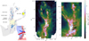 |
Fig. 1 Overview of the morphology and the position of the G202.3+2.5 cloud. Left: schema of the G202.3+2.5 cloud within the context of Mon OB1 East, summarising the results from Paper II. The light gray and light blue areas show the low-density and intermediate-density molecular gas. The five-branch stars mark the positions of the two known open clusters, NGC 2264 and NGC 2259. The four-branch red stars mark the location of groups of protostars. The inward arrows represent the potential global collapse. The outward dashed arrows represent the radiative and mechanical influence exerted by the NGC 2264 open cluster on its surrounding. The insert shows a zoom-in view of the junction region, represented by the hatched area. The triangles mark the location of dense cores. The blue area shows the gas of the filament to the north-east of the junction region. The red area shows the gas of the filament the relates the southern protocluster to the north clump. The directions and red and blue lobes of the two outflows reported in Paper II are also shown. Middle: H2 column density map of the G202.3+2.5 cloud derived from the Herschel/SPIRE data (Montillaud et al. 2015). The lines show the areas of our first IRAM 30-m observations (thin black line; Paper I), of our new IRAM 30-m observations (thick white line), and of our Effelsberg 100-m observations (thick yellow line). Right: zoom-in view of the middle frame with the same colour scale. Black crosses mark the six sources of the GCC catalogue this paper is focussed on. |
Observed emission lines.
2 Observations and data reduction
Here, we present our new datasets obtained with the Effelsberg 100-m and IRAM 30-m telescopes. Table 1 gives an overview of the observed lines, including the IRAM 30-m data obtained in 2017 (Paper I). We are also going to examine the general morphology and dynamics of the region in Sect. 2.3.
2.1 Effelsberg 100-m data
The NH3 mapping of the area was carried out with the Effelsberg 100-m radio telescope in February 2019. NH3 (1,1) and (2,2) inversion lines were observed simultaneously with the 1.3 cm SFK receiver, using the Fast Fourier Transform Spectrometer (XFFTS) backend with a 500 MHz bandwidth. The 17.7 kHz effective spectral resolution gives a velocity resolution of about 0.22 km s−1 at the frequency of 23.7 GHz. 166 points have been observed with 90 seconds ON and 90 seconds OFF times. The 166 points were made on a 15″ grid, covering the brightest area on the Herschel flux density map, represented by the yellow contour in Fig. 1. Deeper observations with 15 minutes ON time were done for six points marking the centre of the GCC sources 1446, 1448, 1450, 1451, 1453, and 1454. The rms noise for the map is 240 mK and 60–80 mK for the deep observations. The beam width of the telescope is 40″ at the frequencies of the NH3 lines, corresponding to a linear scale of about 0.14 pc at a distance of 723 pc.
2.2 IRAM 30m data
The area was first mapped with the IRAM 30-m telescope in March 2017 (black line in Fig. 1). The 13CO, C18O, 12CO, and N2H+ ground transitions were observed and were reported in Papers I and II (see Table 1). Further measurements were done with the IRAM 30-m telescope in May 2019 using the Eight MIxer Receiver (EMIR) receiver to a new set of transitions, as well as with improved spectral resolution in the case of N2H+. The 12 × 5 arcmin2 area represented by the white rectangle in Fig. 1 covers most of the junction region. To cover the molecular tracers (as summarised in Table 1), the area was mapped using on-the-fly observations with three different setups. The first setup targeted the 13CO and C18O J=1−0 lines using the VErsatile Spectrometric and Polarimetric Array (VESPA) autocorrelator with a resolution of 20 kHz (~0.06 km s−1). The Fast Fourier Transform Spectrometers (FTS) autocorrelator was set to observe simultaneously the 12CO (J=1−0) and CS (2−1) lines at a much lower resolution of 200 kHz (~0.6 km s−1). In the second setup, VESPA observed the N2H+ (1−0) lines. In the third setup, VESPA targeted the HCO+ (1−0) line while the FTS autocorrelator was able to detect SiO (2−1) and NH2D. The target rms noise levels were 200 mK, 100 mK, and 100 mK in  scale at the VESPA resolution in setup 1, 2, and 3, respectively. All observations were performed in the frequency-switching mode with a frequency throw of 7.9 MHz, a dump time of 0.2 s, 9″ between rows, a scanning speed of 21″/s leading to ~8.5″ between points along a scan. Sky calibrations and pointing corrections were done at most every 10 minutes and 1.5 h, respectively. The pointing accuracy was found to be generally better than 5.″ The conversion from
  to TMB was done following the IRAM documentation1 with the equation
  , where Feff = 0.95 and Feff = 0.81. The beam width of the telescope ranges from 21″at 115 GHz to 31″ at 77 GHz, corresponding to linear scales of about 0.07–0.11 pc at a distance of 723 pc.
The broad passband of IRAM observations with the FTS autocorrelator (16 GHz of passband in each setup) enabled us to detect approximately 15 lines simultaneously, 9 of which are analysed in the present study. For each line, the data were extracted for typically the 80 km s−1 range about the line and processed independently. For the baseline removal, masking windows were set manually, and the baseline was fitted with a second-order polynomial. The spectra of lines observed with VESPA and FTS were resampled onto 0.06 km s−1 and 0.6 km s−1 channels, respectively. The maps were then computed with the xy_map method of CLASS. Due to the frequency switching mode, the raw baselines were very irregular. For narrow and bright lines they could be removed easily. However, for lines with low S/N and broad profiles (e.g. for methanol, deuterated ammonia and SiO), the baseline removal was very difficult. For these lines the uncertainties are therefore significantly larger than for bright lines like HCO+ or N2H+.
2.3 Maps
Figure 2 shows the ammonia (1,1) and (2,2) integrated intensity maps, the (1,1) first moment map, and (as later detailed in Sect. 3.1) the kinetic temperature map derived from the ammonia observations. It also shows the N2H+, HCO+, CH3OH, SiO, N2D+, and o-NH2D integrated intensity and first moment maps for the junction region. The Her schel compact sources identified by Montillaud et al. (2015), as well as bright spots visible in SiO (northern) and CH3OH (southern), are denoted by black and red crosses, respectively. N2H+ is formed when CO is depleted, outlining the dense gas of the region (e.g. Jørgensen et al. 2004; Yu et al. 2018) Therefore, an N2H+ intensity contour at 1 K km s−1 is used as a reference for all the other maps to facilitate comparison. This contour delineates the dense ridge of the junction region along which lie five Her schel compact sources. It also shows an extension to the north-east of the source 1450 (hereafter the ‘north-eastern extension’), along part of the north-eastern filament. In N2H+ the brightest sources are 1446 and 1450; 1451 and 1453 are less pronounced, while 1448 has no particular shape, no compact source can be seen at its coordinates. In the N2H+ velocity map the velocity gradient outlined in Paper II can be clearly seen: the main filament with velocities of 7-12 km s−1 along the compact sources, with the north-eastern filament with lower velocities merging into 1450.
The brighter areas on the NH3 (1,1) integrated intensity map are well outlined by the N2H+ 1 K km s−1 contour. On this map the brightest source is 1450, and the other sources appear fainter. The velocity gradient visible on the NH3 velocity map is less pronounced than in N2H+. The NH3 (2,2) integrated intensity contrasts significantly with the (1,1) map; 1446 is the brightest source, while 1450 appears to be less strong, The morphology of the kinetic temperature map seems practically unrelated to the contrast between the (1,1) and (2,2). Instead, its morphology is very similar to that of the τm map of the (1,1) emission (not showed). We see lower kinetic temperatures for 1448 and 1451 than for the other sources and the map does not show the trends that may have been expected from the map of dust temperature, Td, as the higher temperature of 1446 (Td=17.1 K, Paper I) and the lower temperature of 1450 (Td=9.9 K, Paper I) do not appear in Tkin. There appears to be higher kinetic temperature around the CH3 OH bright spot, but that might be due to noise and the location close to the edge of the mapped area.
In contrast with N2H+, HCO+ traces intermediate volume densities and is therefore a tracer of more external layers of gas. The integrated intensity of HCO+ is in general agreement with that of N2H+ with notable exceptions: HCO+ is brightest around 1446, while 1450 and 1451 are equally bright. In addition, 1453 seems to form a ridge and not a compact source and it appears weaker in intensity compared to 1451. Again, no compact emission can be seen around 1448. In the HCO+ velocity map, the same gradient can be seen along the ridge as in N2H+, but here it is less pronounced. There is contrast in the north-eastern extension: a red spot can be seen instead of the blue extension visible in N2H+. This red spot seems to correspond to the 11.4 km s−1 contour of Fig. 12 in Paper II, where it was interpreted as a part of an outflow from 1446.
Methanol emission fills almost the whole N2H+ contour, except at its southern end, around source 1451. However, the morphology of its emission is dominated by three bright features. A bright spot is visible near source 1446, where the most evolved protostar (Class I) of this region is located. A second bright spot, marked by a red cross, appears to the north-east of 1446, along the direction of one of the two outflows from 1446 reported in Paper II (along ‘cut 2’ in their Fig. 12). The brightest CH3OH emission is detected in a third spot, also marked by a red cross, located within the north-eastern extension. Its location matches that of the other outflow from the source 1446 (along ‘cut 1’ in Fig. 12 of Paper II) and its velocity in methanol is much larger than in N2H+, similarly to what we noted for HCO+. Interestingly, this spot is connected to the source 1450 via a bright CH3OH linear structure, suggesting it could actually correspond to an outflow from 1450, contrary to the interpretation given in Paper II. We note that a last, less prominent compact source appears next to the source 1448, which is suspected to be protostellar (Montillaud et al. 2015).
The SiO emission resembles that of the bright methanol features, strengthening the idea that shocks are occurring in these places, leading to the desorption of CH3 OH. The SiO velocity map also shows similar structures in velocity to the CH3 OH map, particularly around the SiO bright spot, and the changes in velocity along the sources from 1446 to 1450. The SiO and CH3 OH bright spots seem to be independent of both NH3 (1,1) and (2,2) integrated intensity, consistent with the idea that these points have low density while ammonia traces relatively high- density gas.
Here, N2D+ is the brightest around 1450 and 1453, the latter showing an elongated structure. The rest of the sources do not show up as compact sources and are fainter. The velocity map shows an increase in velocities from 1450 to 1453, consistently with the velocity gradients observed with other tracers. Then, o-NH2D is the brightest around 1450 and 1446. The other sources do not show any structure. The velocity map does not show any structure either, with only a slight increase in velocities from 1450 to 1453.
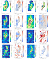 |
Fig. 2 NH3 (1,1) integrated intensity and first moment maps, NH3 (2,2) integrated intensity and kinetic temperature maps, N2H+, HCO+, CH3OH, SiO, N2D+, and o-NH2 D integrated intensity and first moment maps (from top left to bottom right). The white contours on the intensity maps and the black contours on the velocity maps mark N2H+ intensity contours at 1 K km s−1. The black crosses mark the compact sources from the GCC catalogue. The red crosses mark the brightest spots in SiO (northern) and CH3OH (southern). |
Target properties derived from Herschel observations from the source catalogue (Montillaud et al. 2015).
3 Data analysis
3.1 NH3
3.1.1 HFS structure
The NH3 data reduction was performed with the CLASS package of GILDAS2. Following the method of Wienen et al. (2012), for each observed position, we performed an initial fit using the CLASS method NH3(1,1) to determine appropriate windows around hyperfine components for the baseline removal (polynomials). These windows were then used for method NH3(1,1) for the (1,1) lines, and method gauss Gaussian fits for the (2,2) lines. The method NH3 fits assume Gaussian profiles and the same excitation temperature for all hyperfine structure components, and the main group opacity is limited to the range of 0.1–30. The fit gives the following parameters: 1) the product of the optical depth of the main line (τm) times the excitation temperature minus background temperature, 2) radial velocity, 3) the full width at half maximum (FWHM) of a Gaussian profile (∆υ), and 4) the optical depth of the main line (τm) with their respective error estimates. We computed the maximum main beam temperature and the signal-to-noise ratio (S/N) from these parameters. We obtained the rms noise of the spectra from the baseline fitting in CLASS. Three sources (1446, 1453, and 1454) had a single detected NH3 component and the other three sources (1448, 1450, and 1451) had two NH3 components. The mapping observations were finally combined with the xy_map method of CLASS to create maps with 10-arcsec pixels. From these data, we derived the rotational and kinetic temperatures, the NH3 column density, as well as the volume density with the methodology presented in Appendix A.
3.1.2 Line width, velocity dispersion, and gas pressure ratio
The width of the NH3 inversion lines results from the combination of thermal and non-thermal motions. The thermal line width is related to the kinetic temperature through
 (1)
(1)
where Tkin is the kinetic temperature, k the Boltzmann constant, and  is the mass of the ammonia molecule, while mH is the mass of a proton. The line width relates to the velocity dispersion, σv, as
  . The non-thermal velocity can be estimated using
  , where ∆υ is the observed line width and ∆υth the thermal line width.
From the thermal and non-thermal (or turbulent) line widths we obtain the gas pressure ratio (Urquhart et al. 2015) to show the relative contribution of thermal and non-thermal components in the gas pressure:  .
.
3.1.3 Virial parameter
Assuming virial equilibrium, the virial mass of a core of uniform density can be calculated using the NH3 (1,1) line width (Rohlfs & Wilson 2004) as  , where the line width ∆υ(1,1)corr is corrected for the resolution of the spectrometer
  and R is the radius of the source in pc. This equation neglects the magnetic energy. For our calculations, we are assuming a spherical core, and we are not including external pressure. We assume a power-law profile (ρ ∝ R−1.5, see Appendix A.3 in Paper I). The virial parameter is
  , which is ≲2 for clumps gravitationally bound and potentially collapsing cores (Bertoldi & McKee 1992). For Mgas, we used the average of the mass estimates from dust observations. The values of gas mass and source size used to obtain the virial mass and virial parameter are given in Table 2.
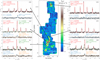 |
Fig. 3 N2H+ integrated intensity map (Montillaud et al. 2019a) with the NH3 spectra of the sources of the deep observations. The colours on the plots of the spectra separate the identified components and their parameters. Red: (1,1) first, stronger component, green: (1,1) second, weaker component, blue: (2,2) first, stronger component, orange: (2,2) second, weaker component. |
3.1.4 Uncertainties of the physical parameters
We performed Monte Carlo (MC) simulations to derive the uncertainties of the physical parameters from the observational uncertainties and to check the shape of the error distributions. The hyperfine structure fit of the NH3(1,1) line and the Gaussian fit of the NH3(2,2) line presented earlier were repeated in Python using the curvefit function to obtain the corresponding covariance matrices. These matrices and the errors obtained originally from CLASS were then fed to a multi-variate Gaussian random number generator to simulate, for each core, 1000 mock spectra parameters (Tant × τ, υLSR, FWHM(1,1), τm for NH3(1,1); Area, υLSR, FWHM(2,2) for NH3 (2,2)) with realistic distributions. From these parameters we derived distributions of core physical parameters: NH3(1,1) and NH3(2,2) main beam brightness temperatures, kinetic temperatures, column densities, H2 volume densities, thermal and non-thermal line widths, gas pressure ratios, and virial parameters according to the equations outlined in Sect. 3.1. The standard deviation of the distribution of each parameter was considered as an estimate of its uncertainty. Points with rotational temperature outside the 0–50 K range, or Ntot outside the 0–1017 cm−2 were deemed nonphysical and were excluded from the standard deviation calculation. Figure 4 illustrates that in spite of the non-linearity of the equations the final distributions are close to Gaussian shapes, which justifies the use of standard deviations to represent uncertainties.
3.2 N2H+, N2D+, and NH2D data analysis
The N2H+, N2D+, and NH2D spectra were analysed using the CASSIS software (Vastel et al. 2015). Excitation temperatures, column densities, central velocities, and line FWHM were evaluated using Markov chain Monte Carlo (MCMC), where the acceptance of a step is determined by the value of the χ2 difference between the model and the observations. Here, the observations consist of individual spectra obtained by averaging the IRAM position-position-velocity (PPV) cubes over the source area defined from the Herschel maps in the GCC catalogue. The source angular sizes were fixed to 70″, the typical size of these sources in the GCC catalogue, because we observed that the MCMC was not able to constrain this value, which acted as a nuisance parameter when we let it free.
We used the LTE model with one component to fit 1453, and two components to fit 1446, 1448, 1450, and 1451 in the case of N2H+. For the deuterated species, the S/N was too low to disentangle two components, thus, the entire analysis was performed assuming a single component. The model requires initial values and lower and upper limits for the following input parameters: molecular column density, excitation temperature, line FWHM, source angular size, and VLSR. Table 3 lists the values that we adopted. The script uses one walker which makes 100 000 steps during a run. The first half of the chain was considered as burnin and was dropped. We set step sizes (the ‘rpp’ parameter) to get the acceptance rates between 0.2 and 0.5. We repeated the MCMC chains ten times for each source to assess the stability and reproducibility of the results.
In the case of N2H+, we explored the impact of the initial excitation temperature on the MCMC, and observed that it favoured the excitation temperature we fed it. The χ2 values were found to be slightly better at low temperatures (~5 K), mostly due to a better fit of the line width that was obtained that way. We conclude that our N2H+ data, with a S/N value between 6 and 18 for the isolated component, is not sufficient to firmly constrain the excitation temperature. We adopted the 5 K value for the initial excitation temperature and left this parameter free in the MCMC. This value is broadly consistent with the excitation temperatures obtained from NH3 data. We assumed the same initial excitation temperature of 5 K for the other species.
Initial values and boundaries for the CASSIS MCMC.
4 Results
We present the NH3 pointed observations in Sect. 4.1, and the IRAM 30-m data on the compact sources in Sect. 4.2. Results on the dynamics of the region are presented in Sect. 4.3.
4.1 NH3 deep observations
Figure 3 shows the NH3 spectra of the compact sources observed with a longer integration time (see Sect. 2.1). Three sources had a two-component NH3 spectrum and three sources had a singlecomponent spectrum. We detected the hyperfine structure for all (1,1) measurements with significant S/N, however, we only detected the main hyperfine group of the (2,2) lines. We obtained high S/N values for the (1,1) lines ranging from 5.9 to 8.9 for the weaker velocity components and from 24.4 to 31.5 for the stronger velocity components. As for (2,2) lines we obtained weak S/N ratios for the weaker components between 1.6 and 3.6. For the stronger components, the S/N ratios range from 4.0 to 8.1.
The (1,1) spectrum of 1446 shows a wing on its blue-shifted side. For 1448 we see small lobes on both sides of the hyperfine structure, which were masked out to obtain a reasonable fit in CLASS. The second component of 1450 seems to be an uncertain detection, its hyperfine groups aside from the main component are barely detectable. Its main hyperfine component however, compared to the shape of e.g. the wing of 1446 made it reasonable to try fitting a second component. Having a second component for 1450 resulted in a more acceptable line width for its stronger component, improving the fit altogether.
Tables D.1 and D.2 show the parameters obtained from CLASS and the subsequent Python refit. Table D.3 shows the physical parameters obtained from both transitions. The uncertainties in both tables come from the MC simulations outlined in Sect. 3.1.4.
The NH3 (1,1) brightness temperatures range from 0.4 K (1450, weaker component) to 2.36 K (1453). If we only look at the first, stronger components, then the lowest value is 1.46 K (1448). Their uncertainties range from 0.03 to 0.06 K. The NH3 (2,2) brightness temperatures range from 0.94 K (1450, weaker component) to 0.45 K (1446). Among the stronger components, 1451 has the lowest (2,2) brightness temperature with 0.25 K. We obtained uncertainties between 0.02–0.05 K, and a large uncertainty for the weaker component of 1450 with 0.94 K.
We obtained kinetic temperatures between 10.0 K (1454) and 20.4 K (1448) with uncertainties between 0.2 and 6.0 K. Excitation temperatures range from 3.7 K (1451, second component) to 7.9 K (1451, first component) with uncertainties between 0.07 and 2.9 K. We obtained NH3 column densities between 2.5 × 10¹⁴ and 1.9 × 1015 cm−2 with uncertainties between 8 × 10¹³ and 1.2 × 1015 cm−2. Comparing these column densities to the H2 column densities from Paper I provides estimates of ammonia abundance in our targets. Figure 5 illustrates that the values we obtain are within the range of literature values. The H2 volume densities range from 2.3 × 10³ to 2.2 × 104 cm−3 with large uncertainties between 3.4 × 10² and 5.5 × 104 cm−3.
The ratios between thermal and non-thermal gas pressures range between 0.035 and 0.143, with uncertainties between 0.002 and 0.214, the latter belonging to the weaker component of 1450. The low values imply the dominance of non-thermal motions in the sources. Virial parameters range between 0.03 and 0.367, with uncertainties between 0.002 and 0.029. To imply that a source is gravitationally unstable, α ≪ 2 is needed, which applies to all of our sources. However, when calculating the virial parameters, we have not taken the effect of the magnetic field into account and it may contribute to support the cores against infall (Bertoldi & McKee 1992; Kauffmann et al. 2013; Evans et al. 2021). That is also the opposite what we observed at moderate density cold cores where Tdust > Tkin (e.g. Tóth et al. 2000). Since dust and gas are expected to be effectively coupled at densities higher than 104.5 cm−3 because of frequent collisions between dust grains and gas particles (e.g. Goldsmith 2001), we might have expected to obtain a good correlation between kinetic and dust temperatures, especially for the densest and coldest sources. Figure 6 shows that there is indeed a good correlation between the two temperatures in our sample, but there is a significant trend that sees kinetic temperatures growing larger than dust temperatures for lower temperature sources. This trend is especially striking for the source 1450, with a low kinetic temperature and high column and volume densities (for the stronger NH3 component). For this source, we got ~14 K for kinetic temperature while having ~10 K as dust temperature, and 8 × 1022 cm−2 H2 column density. This situation contrasts with many studies (e.g. Forbrich et al. 2014; Friesen et al. 2016; Sokolov et al. 2017), but it is not unusual. For example, based on NH3 data, Merello et al. (2019) found high Tkin/Tdust values in Hi-GAL prestellar clumps (sizes ~0.1- 1 pc). The main heating source for these clumps is cosmic ray heating and (to a lower extent) UV heating. They found an overall agreement between NH3 derived Tkin and T dust at volume densities n ≳ 1.2 × 104 cm−3. In prestellar clumps, they found a median Tkin /Tdust =1.24, suggesting that those sources are thermally decoupled. Our source 1450 exhibits a value of Tkin /Tdust =1.4. To further clarify the nature of this source and the NH3 measurements, we analysed the additional molecular data. We discuss these results regarding the NH3 data in Sect. 5.1.2, and 1450 in Sect. 5.3.1.
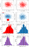 |
Fig. 4 Results of the MC simulations for 1446. Frames a, b and c show parameters obtained for the NH3 (1,1) line, c and d for the (2,2) line. Frames e and f show the distribution obtained for main beam brightness temperature, TMB(1, 1) and TMB(2, 2), g for rotational temperature and h for the NH3 column density. Black crosses mark the values obtained from the CLASS fitting. The black thick dashed lines show the values obtained with the best fit parameter, the black thin dashed lines show the standard deviation, and the red dashed lines indicate the 16th, 50th, and 84th percentiles. |
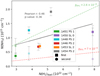 |
Fig. 5 NH3 column density vs H2 column density from the GCC catalogue (Montillaud et al. 2015). The dashed lines indicate NH3 abundance values: green dashed line: 2.6 × 10⁻⁸ (Harju et al. 1993, Orion & Cepheus NH3 clumps, median); red dashed line: 7 × 10⁻⁹ (Wienen et al. 2018, ATLASGAL sample, lowest value). The columns of the legend: (1) source name (2) source type: PS: protostellar source, SL: starless source (3) reliability of source classification: 0: unreliable, 1: candidate, 2: reliable. The square marks denote the stronger component, the circle the weaker component of the source. |
4.2 IRAM 30-m view of the compact sources
Figure 7 and Appendix C.1 show the spectra for all the tracers observed with the IRAM 30-m telescope, for each compact source and the two bright spots in SiO and CH3 OH (panels 3–4 in Fig. 7). We decompose the presentation of the results into several subsections, starting with the intermediate density tracers, then moving to the high density tracers and deuterated species, and we conclude with the shock tracers.
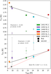 |
Fig. 6 Relationship between temperatures derived from NH3 and dust temperature. Top: NH3 (1,1) main beam temperature as a function of dust temperature (Montillaud et al. 2015). Bottom: kinetic temperature as a function of dust temperature. The red dashed line marks the 1–1 correlation line. The grey line of the least square fit slope is far from 1, two sources with dust temperatures below 10 K have significantly higher kinetic temperatures. The legend is the same as in Fig. 5. |
4.2.1 Intermediate density tracers
In terms of 12CO, we see that our sources have an asymmetric spectrum with a blue-shifted wing. The exceptions are 1454 and the CH3OH bright spot. 1454 has a small second component on the blue-shifted side, and its main component is rather symmetric. The CH3OH bright spot has an extended red-shifted wing.
The 13CO and C18O spectra show multiple components for 1448, 1450 (with possible self-absorption) and 1451 coinciding with the velocities of the NH3 components. We see the two components in HCO+ as well as for 1450 and 1451. The CS spectra are rather symmetric, except for 1451, which has an extended red-shifted wing, as well as for the CH3OH bright spot, where both CS and HCO+ show an extended wing similarly to its 12CO spectrum.
4.2.2 High-density tracers
The CASSIS results obtained for N2H+, N2D+, and NH2D are summarised in Table 4. The obtained reduced χ2 values are in the range of 0.7–2.7, indicating a satisfying match between the model and the observations. The corner plots used to assess the quality of the fit parameter estimated by CASSIS are presented in Figs. E1–E4. We see that N2H+ is very well detected in all the GCC sources, with a S/N of the isolated hyperfine component of 6.3 for 1448 and 18.2 for 1453. The velocity of this transition is well aligned with the velocity of the NH3 lines. Diazenylium remains completely undetected for the SiO bright spot, and we see two components at the CH3OH bright spot. This difference between the two spots is consistent with the fact that the SiO spot is rather off the filaments, while the methanol spot falls on the beginning of the north-eastern filament. Then, N2D+ and o- NH2D are detected in all the GCC sources, however with very low intensities: N2D+ and o-NH2D are approximately 10 and 5 times weaker than N2H+, respectively. Consequently, their S/N are very low and the baseline subtraction was difficult and sometimes very poor, for instance, for 1448. The consistency of the integrated emission maps in Fig. 2 supports the idea that the detections are real. The velocity range in Fig. 7 and Appendix C.1 was chosen to compare the different transitions. A better view of the spectra with hyperfine components can be seen in the top right frames of Figs. E1-E4. These transitions are undetected for both bright spots, indicating the lack of dense material in these locations. The velocities of N2D+ and o-NH2D do not align with the velocities of either of the NH3 components, except in 1448, where o-NH2D seems to align with the velocity of the weaker NH3 component. This indicates that the gas layers traced by ammonia and deuterated species are different.
Properties of N2H+, N2D+, and o-NH2D lines from the CASSIS MCMC fit.
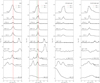 |
Fig. 7 Spectra of the observations to the GCC sources 1446 and 1450, and to the coordinates of the brightest SiO and CH3 OH emission, as indicated in the top-right corner of each frame. The red and green vertical lines denote the velocities of the NH3 (1,1) first (stronger) and second (weaker) components, respectively. |
4.2.3 Deuterium fractionation
Figure B.1 shows the MCMC column density distributions obtained with CASSIS (Sect. 3.2) for N2H+, N2D+, NH3, and o-NH2D, as well as the derived distribution of deuterium fractionation defined as the ratio of these column densities: N(N2D+)/N(N2H+) and N(o-NH2D)/N(NH3) (Busquet et al. 2010). The interest of this approach is to take advantage of the MCMC distributions to estimate the distribution of possible fractionation values and extract the maximum information available in the low S/N data of deuterated species. It helps in identifying the sources where the deuteration fraction is very uncertain, as 1451 for diazenylium and 1448 for ammonia, and reveals different regimes, 1446 being less deuterated than the other sources in diazenylium, and 1450 being more deuterated than the average in ammonia. When several velocity components were detected in the normal molecule and not in its deuterated counterpart, only the brightest component was used. The deuterium fractionation in our targets spans very different ranges in the two molecules analysed here: from ~0.1 for 1446 to ~0.5 as an upper limit for 1450 in diazenylium, and from ~0.005 as a lower limit for 1451 to ~0.8 as an upper limit for 1450. We discuss these values in Sects. 5.2.1 and 5.2.2.
4.3 Tracing the dynamics of the junction region
4.3.1 Infall diagnosis
Mardones et al. (1997) proposed a method to detect cores and clumps that may be infalling. This method was later on used by Lee et al. (1999). The method is based on the comparison of line profiles between an optically thin tracer and an optically thick one. The optically thin tracer is used to estimate the systemic velocity. The optically thick one is sensitive to the radiative transfer effects and is more prone to carry the information about the core dynamics. We performed this infall diagnosis for N2H+ and HCO+, which presents the advantage that both are molecular ions and therefore similarly sensitive to magnetic fields, so that the differences between the two lines are more likely to reflect the core dynamics.
The N2H+ line is a typical tracer for somewhat higher density gas because it forms only at high ISM density, making it a good tracer of the innermost parts of the target and, therefore, of its systemic velocity. In contrast, HCO+ may also form in diffuse molecular environment (Turner 1995).
The amount by which the HCO+ line is red- or blue-shifted compared to the N2H+ line is given by the normalised velocity difference  . A significant blue-shifted asymmetry is interpreted as a possible infall signature, arising from a so-called inverse P-Cyg profile, where the optically thick tracer is typically double-peaked (with one peak on each side of the optically thin tracer velocity).
The results of the infall diagnosis are shown in Fig. B.2 for the junction region and in Appendix F for a global view of the region, along with zoom-in views to the compact sources southwards of the junction region. To get the values we used 3×3 pixels for each point, averaging their values to obtain a spectrum and, thus, a point in the  colour map. The figures reveal a contrasted situation, where most of the junction region is blue-shifted, especially about the densest and most massive source, 1450. The outer parts of the junction region and the southern compact sources (Fig. F.2) are rather red-shifted. These results are consistent with the idea that the densest parts of the junction region are collapsing, while the surrounding may correspond to transient structures.
On the other hand, the junction region spectra generally do not present a typical inverse P Cyg profile, since the HCO+ line mostly peaks at the same velocity as the N2H+ line. In these cases, the blue asymmetry may occur accidentally from a distinct velocity component.
Important exceptions are the pixels #51 45 to #51 51, where the HCO+ peak is clearly blue-shifted compared to N2H+. A shoulder is visible on the red side, making these pixels good infall candidates. Interestingly, source 1450 is located within the middle of this range of pixels. We cannot exclude, however, that these features arise from multiple velocity components. In a few cases, we judged the diagnosis to be unreliable and marked the infall map with a cross in Fig. B.2. This is the case, for instance, at location # 48 54, where the low S/N of the N2H+ line prevented a good fit, or at location # 54 42, where the presence of two distinct N2H+ components made the asymmetry estimate unclear.
4.3.2 Shock tracers
The spatial distribution and the velocities of SiO and CH3OH are shown in the second row of Fig. 2. The integrated intensity map of SiO is reproduced in Fig. 8 and shows the directions of the two crossed outflows from 1446 reported in Paper II. The SiO emission appears strongest in one of these two outflows. It is detected in 1450, 1448, and 1446 along the ridge of the junction region, and we do not detect it in 1451 and 1453. Figure 9 shows the tight correlation between SiO peak temperatures and CH3OH peak temperatures for the three GCC sources with SiO detection. In Fig. 10, we show the peak temperatures as a function of the gas pressure ratio calculated from NH3 line widths, as we may expect that a strong shock pressure may result in a lower value of the thermal to non-thermal gas pressure ratio, Rp. However, Fig. 10 shows no clear correlations between the SiO or methanol lines and the Rp parameter.
Figure 8 shows the SiO spectra for three regions defined by an isocontour in the SiO integrated intensity map at the level of 0.77 K km s−1 in TMB scale. The three regions are represented by the red contours in the inset of Fig. 8. Interestingly, the elongated shape of the 1450 bar is suggestive of an outflow and intersects with the direction of one of the two 1446 outflows at the location of the methanol bright spot. Figure 8 shows that the SiO line widths are much larger than for the other tracers, with FWHM of 9.0 km s−1, 8.5 km s−1, and 4.8 km s−1, respectively, consistent with the idea that this SiO emission is related to shocks. The SiO spot contrasts with the other two regions by its greater peak and integrated intensities, as well as by its smaller FWHM and its symmetrical line profile. It is well fitted by a Gaussian function, while the other two regions present notably skewed profiles. We fitted them with a skew normal distribution:
 (2)
(2)
 (3)
(3)
 (4)
(4)
 (5)
(5)
where υ, υ0, and σ have their usual meaning for a Gaussian line fitting and α is the so-called ’shape’ of the distribution that characterises the asymmetry of the distribution. It is related to the skewness, γ, by the relation:

The skewness values we obtained are 0.79, 0.79, and 0.08 for the three regions, respectively, confirming that the first two regions are significantly skewed, while the SiO spot is only marginally skewed.
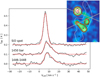 |
Fig. 8 SiO (2–1) spectra for the three main SiO bright regions (thick grey lines). The red lines show the Gaussian best fit for the SiO spot region, and the skew normal distribution best fit for the other two regions. The insert reproduces the integrated intensity map of SiO shown in Fig. 2. Red contours were added to show the regions where the SiO spectra were considered (SiO spot, 1446–1448, and 1450 bar, from north to south). The grey lines represent the outflow directions from 1446 according to Paper II (their Fig. 12). |
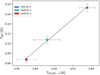 |
Fig. 9 Correlation between the peak temperatures of SiO (2–1) and CH3OH in the three GCC sources where these transitions were detected. |
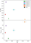 |
Fig. 10 Relationship between shock tracer temperatures and gas pressure ratio. Top: SiO main-beam peak temperature as a function of gas pressure ratio calculated from NH3 line widths. The arrows mark the upper limits of SiO detection of the sources 1451 and 1453. Bottom: CH3OH peak temperature as a function of gas pressure ratio calculated from NH3 [line widths]. The columns of the legend are as in Fig. 5. |
5 Discussion
In this section, we discuss three main questions. In the first part, we compare the data obtained from the various molecules to identify the relevant density tracers for this region. In the following part, we take a close look at the deuteration of ammonia and diazenylium in G202 and put it in perspective with the data reported in the literature for other regions. Finally, we examine whether putting all our data together helps us in proposing a scenario on the nature, origin, and fate of the G202 junction region.
5.1 Considering the relevant dense gas tracers in G202
5.1.1 Correlations between ammonia and other tracers
Figures B.3 and B.4 display the correlations between ammonia line characteristics and derived physical parameters with the main beam peak temperatures of 12CO, 13CO, C18O, CS, and N2H+. Figure B.3 shows that there are no correlations between N2H+ and the parameters from NH3 analysis. This could imply that in our sample the NH3 emission is dominated by densities just below 104 cm−3, namely, before N2H+ can be abundant. The optical depth of ammonia may also play a role, although the transitions are only marginally thick with values in the range τ ~ 0.5–1.5, except for the GCC source 1454 where τ = 3.24. The correlations of ammonia line characteristics with CS look very similar to those with 12CO, which contradicts the notion that CS would be a good density tracer. The fact that 12CO peak temperature is so similar to NH3 kinetic temperature (Fig. B.4) also indicates that NH3 does not probe the densest layers of this cloud.
The anti-correlation between C18O peak temperature and NH3 kinetic temperature is particularly tight. It could reflect the other typical limit case, that is when a line is optically thin, as C18 O is here. Then its brightness temperature reflects the column density. More generally, in our sample, C18O peak temperature appears as a good predictor of the three physical quantities represented here, Tkin, Rp, and α.
Other noticeable correlations are between the peak temperatures of 12CO and CS, and the gas pressure ratio obtained from NH3 [line widths]. All these elements point to the idea that in G20212 CO, 13CO, CS, and even ammonia tend to trace low to intermediate density layers of gas. The fact that diazenylium becomes abundant only when polar molecules like CO or CS freeze out on dust grains makes this molecule the best bright tracer of dense gas. To go beyond diazenylium-based diagnostics, we discuss deuterated species in the next section. Before that, we take a closer look at ammonia properties.
5.1.2 NH3 in characterising dense gas
The fact that we observe a good correlation between the ammonia-based virial parameter and dust temperature (Fig. 11) and the kinetic temperature we obtained was higher than their dust temperatures (Sect. 4.1) suggests that the estimates of N (NH3) and n(H2) do not include the densest layers so that NH3 is not sufficient alone for the characterisation of gas parameters. This is in line with other studies. For example, Manjarrez Esquivel (2018) pointed out the importance of using different molecular tracers in order to get a more complete understanding of gas parameters of a region.
A limitation to NH3 is that it cannot be used within the central ∼1000 AU of a core because of its relatively low critical density. Additionally, NH3 depletes in the coldest, densest regions of prestellar cores. Even with interferometric studies, NH3 shows depletion in a prestellar core (see Sect. 1). According to recent chemical models of star-forming regions, NH3 freezes out onto grain surfaces at low temperatures and medium densities (T ~ 10K, n ~ a few times 105 cm−3; e.g. Sipilä et al. 2019). Therefore, NH3 may not, in fact, be a good tracer of the gas kinetic temperature in the densest and coldest regions (Friesen et al. 2009). However, in L1544, a prestellar core in Taurus, it has been found that NH3 abundance increases toward the dust peak and shows no sign of depletion in the centre of the core, even though it has high volume density (n(H2) > 106 cm−3, Crapsi et al. 2007). Recent chemical models (e.g. Sipilä et al. 2019) have not been able to reproduce this NH3 profile.
Regarding deuterated ammonia, Caselli et al. (2022) presented the first observational evidence of complete NH2D freeze-out towards the prestellar core L1544 based on ALMA data. Their chemical model coupled with a non-LTE radiative transfer code shows that NH2D already starts freezing out at around a distance of 7000 AU.
These elements explain the inadequacy of ammonia to characterise dense gas when the volume density is very large, but it is unclear whether such high densities are reached in the G202 compact sources. In the case of the densest source of our sample, 1450, no NH3 depletion could be observed, although the low resolution of the Effelsberg 100-m telescope at this frequency may not enable such a detection. Radiative transfer modelling may be necessary to address these questions further but this is beyond the scope of the present study.
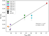 |
Fig. 11 Correlation between the virial parameter from NH3 data and dust temperature. The symbols are is in Fig. B.3. |
5.2 Deuteration in the G202 region and elsewhere
5.2.1 Comparison of NH3 deuteration in the G202 region with other samples
We compared the NH3 deuterium fractionation, Dfrac(NH3), we obtained with other samples from different star forming regions. Table 5 provides a short summary of these samples. Figure 12 shows the NH3 column densities and the NH2D/NH3 deuterium fractionation ratios of these samples with our sample.
We found some disagreement among the various studies reporting Dfrac(NH3) measurements. Following some authors, this quantity could be a good indicator of the evolutionary stage of cores. In their analysis of Plateau de Bure interferometric observations of two high-mass star-forming regions, Pillai et al. (2011) reported that NH2D is destroyed when embedded protostars are present. Similarly, Busquet et al. (2010) observed pre-protostellar cores around the UCHII region in IRAS 20293+3952 and found strong NH2D emission towards starless cores, but didn’t find such emission towards protostellar ones. Regarding low-mass star formation, Li et al. (2021) studied a cluster of low-mass starless and prestellar core candidates in a massive star protocluster-forming cloud, NGC 6334S. They stated that NH2D could be a powerful tracer to reveal the starless and prestellar cores that do not show significant dust continuum emission.
In contrast, Fontani et al. (2015) concluded, based on a sample from high-mass star-forming regions (as in Fontani et al. 2011, see Sect. 5.2.2) that Dfrac(NH3) does not show significant changes across different evolutionary phases and they found the highest values in protostellar sources. In their sample of massive star-forming regions, Wienen et al. (2021) found no correlation between Dfrac(NH3) evolutionary tracers.
Galloway-Sprietsma et al. (2022) observed 22 dense cores in the low-mass star forming region L1251, out of which 20 are starless or prestellar, and 2 contain a protostar. They found no discernible trends in plots of median deuterium fractionation of [o-NH2D]/[p-NH3] with any physical or evolutionary parameters.
Wienen et al. (2021) selected massive clumps from the ATLASGAL survey (Schuller et al. 2009) to observe in o-NH2D at ∼86 GHz and p-NH2D at 74 GHz and at 110 GHz to determine their temperature. They observed 992 clumps, and detected NH2D in 390 clumps with S/N > 3, with the hyperfine structure of o-NH2D at 86 GHz being visible in 79 clumps. Altogether, the authors conclude that they found no correlation between evolutionary phase and NH3 deuteration.
In our sample, the NH3 deuterium fractionation values fall in the range 0.02–0.3. The core 1451, a candidate protostellar core, has the lowest NH3 deuterium fractionation. The massive starless core candidate at the junction of the filaments, 1450, has the highest value. The protostellar cores 1446, 1448, along with the protostellar candidate core 1451, display scattered values. However, according to Fig. 2, the ammonia emission of source 1448 is broadly contaminated by that coming from 1450, which may explain the similar Dfrac values seen for these two sources. The starless core candidate 1453 falls between them all. Regarding NH3 column densities, our sample falls between the low-mass cores of L1251 (Galloway-Sprietsma et al. 2022) and the high-mass ATLASGAL clumps (Wienen et al. 2021), and mostly are similar to those of the pre-protostellar cores of a UCHII region examined by Busquet et al. (2010), and the low-mass cores in the massive star protocluster examined by Li et al. (2021). As for NH3 deuterium fractionation, the difference between the samples seems to be within their scatter. The low-mass core sample of Li et al. (2021) from a high-mass star-forming region has the lowest scatter. The ATLASGAL sample has the biggest scatter of NH3 deuterium fractionation values. These sources are sampled from various environments in the inner Galactic plane.
The values found for our sample are in line with the conclusion of Fontani et al. (2015) and Wienen et al. (2021), finding no correlation between evolutionary phase and NH3 deuteration. The left column of Fig. 13 shows the NH3 deuterium fractionation plotted against NH3 (1,1) line width and rotational temperature, similarly to Fig. 6 of Wienen et al. (2021). They used the NH3 (1,1) line width and rotational temperature as evolutionary phase indicators because Wienen et al. (2012) obtained a statistically significant correlation between these parameters and the evolutionary phase of the source. Similarly to their 2021 study, where they found no correlation between Dfrac(NH3) and these parameters, we find no correlation for our sample either.
Samples used for comparison of NH3 deuteration in the G202 region.
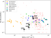 |
Fig. 12 NH2D/NH3 deuterium fractionation ratio versus NH3 column density. Orange marks denote the dense core sample from a low-mass star forming region of Galloway-Sprietsma et al. (2022), blue marks the low-mass sample from a high-mass protocluster in Li et al. (2021), green marks the pre-protostellar cores of a UCHII region in Busquet et al. (2010), red marks the high-mass ATLASGAL clumps of Wienen et al. (2021), and light blue marks with a black outline denote the NH2D cores (squares) and the NH3 cores (stars) from the pre-protoclusters in Pillai et al. (2011). Our sample is depicted by black crosses, showing the estimates for NH3 column density. The downward arrows mark upper limits for the values depicted. Regarding the sample of Wienen et al. (2021), the rounding of values in the CDS table provided by the authors result in many sources having the exact same values. |
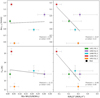 |
Fig. 13 Parameters from NH3 analysis: (1,1) line width and rotational temperature as a function of NH3 and N2H+ deuterium fractionation. The legend is the same as in Fig. 5. The square marks denote the stronger component, the circle the weaker component of the source. For NH3 deuteration, we see no correlation between the parameters. For N2H+ deuteration, we see a correlation between the evolutionary phase of the sources and the rotational temperature. |
5.2.2 Comparison of N2H+ deuteration in the G202 region with other samples
Figure 14 shows the N2H+ and N2D+ column densities of our sample compared to three other samples: high mass cores in different evolutionary stages from Fontani et al. (2011), Class 0 and borderline Class 0/I objects from nearby low-mass star forming regions from Emprechtinger et al. (2009), and low mass starless cores from Crapsi et al. (2005).
These three studies used the IRAM 30-m telescope to observe between 20 and 31 cores each, in N2H+ at 93 GHz and N2D+ at 154 GHz (Crapsi et al. 2005; Fontani et al. 2011) or 77 GHz (Emprechtinger et al. 2009). The distances to the examined regions are different, leading to differences in physical resolutions, as summarised in Table 6. All three studies con- elude that the N(N2D+)/N(N2H+) ratio correlates significantly with evolutionary tracers; for instance, the CO depletion factor (Crapsi et al. 2005; Emprechtinger et al. 2009), the dust temperature (Emprechtinger et al. 2009), or the presence or absence of protostellar objects in the cores (Fontani et al. 2011). The latter authors emphasise that the N2D+ abundance is higher in the prestellar phase, similarly to low-mass star formation it decreases during the formation of the protostar (or protostars), and it stays relatively constant in the UCHII region phase.
In Fig. 14, the low-mass and high-mass nature of the sample does not seem to influence the azenylium deuterium fractionation, all the sample having values typically in the range between 0.04 (average Dfrac of the high mass protostellar objects, and ultracompact HII regions groups, Fontani et al. 2011) and 0.26 (average Dfrac of the high mass starless cores group, Fontani et al. 2011).
The N2H+ deuteration fraction values of our sample fall in the range 0.07–0.32, consistently with the studies discussed above. The Class I/II protostellar core 1446, which is the most evolutionarily advanced source of our sample, has the lowest value. The massive starless or Class 0 core 1450 has the highest value. The starless core candidate 1453 has a similar value to that of 1450. The right column in Fig. 13 shows the N2H+ deuterium fractionation plotted against the NH3 (1,1) line width and rotational temperature considered as evolutionary indicators (Sect. 5.2.1). We see a possible correlation between the N2H+ deuterium fractionation and NH3 (1,1) line width and a significant correlation with the rotational temperature, implying that they trace the evolution of the sources. This is in line with the conclusions of the articles cited above, although with large uncertainties in both cases. These results confirm that all sources but 1446 are in a young evolutionary stage. In Fig. 14, it is striking that all the sources but 1446 fall about the Dfrac average value of high-mass starless cores reported by Fontani et al. (2011), while 1446 is near the Dfrac average value of high-mass protostellar objects.
Samples used for comparison of N2H+ deuteration in the G202 region.
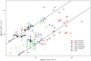 |
Fig. 14 N2D+ column density versus N2H+ column density. Red symbols denote high mass starless cores (HMSCs), high mass protostellar objects (HMPOs), and ultracompact HII regions (UCHIIs) from Fontani et al. (2011), blue circles denote Class 0 objects from Emprechtinger et al. (2009), and green circles denote low mass starless cores from Crapsi et al. (2005). Our sample is indicated with thick black crosses. The two solid black lines indicate Dfrac values of 0.26 (average Dfrac of the HMSC group) and 0.04 (average Dfrac of the HMPO and UCHII groups), similarly to Fig. 1 of Fontani et al. (2011) to aid comparison. |
5.3 Considering the nature of G202
The original motivation for this study was to unveil the exact nature, origin, and fate of the G202 massive clump, following Montillaud et al. (2019b), who showed that it corresponds to the junction between two colliding or inflowing filaments. In particular, we question whether this clump is gravitationally unstable: whether it arose from the global gravitational collapse of its parent molecular complex or from a fortuitous collision between filaments pushed by the expansion of the cavity powered by the massive star S Mon, a few parsecs southwards. In this last discussion section, we examine how the elements presented above help understanding the nature of two sources of the region to shed some light on these questions.
5.3.1 1450: a massive core at the confluence of two filaments
1450 is the source that surpasses all the G202 sources in almost every physical quantity. It is the only source detected in all the molecular tracers studied in this work and in dust continuum (Juvela et al. 2010; Montillaud et al. 2015) from 100 µm to 500 µm. It is also the brightest seen in most data. According to Papers I and II, it is shown to be the most massive (52 M⊙), densest (with a column density of almost 1023 cm−2), among the coldest (Tdust ≈ 10 K), and the most gravitationally bound ( and 1.0,
  and 0.5, and
  and 0.04 for the components at υLSR ≈ 7.2 and 5.6 km s−1, respectively). We found here that it is also the most deuterated source, both in ammonia and diazenylium, the latter suggesting that it might be closest to the onset of gravitational collapse (Sect. 5.2.2).
It is likely that the location of the core 1450 close to the junction of the two colliding filaments is related to these physical and chemical characteristics. In Section 4.3.1, we found that the only region with important signs of gravitational infall is the immediate surrounding of this source. It also presents unique characteristics in the shock tracer maps of SiO and methanol, with a ∼0.3 pc-long linear structure from 1450 to the methanol bright spot north-east of it. The linear shape of this structure suggests that it might be an outflow from a possible embedded protostar. In Fig. 15, we show some contours of the SiO emission integrated on the velocity range 3.0–6.75 km s−1 in blue and 7.0– 15.75 km s−1 in red, while the optically thin N2H+ and N2D+ emissions peak approximately at 7 km s−1. The bipolar distribution of the red and blue contours about this source support the outflow hypothesis. The evolutionary stage of 1450 remained undetermined in our previous studies, the range of possibilities spanning from starless to Class 0. The SiO data rule out the starless hypothesis. An evolutionary stage later than Class 0 seems unlikely, considering the lack of a mid-IR detection. The youth suggested by diazenylium deuteration and the compact source detected at 100 µm point to a young Class 0 object. The extent of the outflow (∼0.3 pc) is somewhat surprising compared to the typical scales of 0.05 pc reported by Duarte-Cabral et al. (2013) for massive Class 0 to Class I protostars in Cygnus- X with masses in the range ∼10 – 50 M⊙. A puzzling element is the strong asymmetry of the structure with respect to 1450. Interestingly, the situation is similar to that reported for 1446 in Paper II, with a long red outflow to the east and a short blue outflow to the west. Another peculiarity is the modest FWHM of 8.5 km s−1 in the SiO line profile of the 1450 bar displayed in Fig. 8, which suggests that it takes its origin in a shock whose velocity has a similar order of magnitude. To get an alternative estimate of the shock velocity, we can follow Louvet et al. (2016) and compare the SiO line integrated intensity to the predictions of the Paris-Durham shock models, as reported in their Fig. 8. In the 1450 bar, we measured an SiO integrated intensity of 1.1 K km s−1 ; according to the chosen model assumptions, this could correspond to shock velocities between 7 and 11 km s−1. According to Louvet et al. (2016), this falls in the range of low velocity shocks, which they interpreted as a signature of converging flows in the case of the W43-MM1, a much more massive ridge than G202. In our case, the SiO emission spreads to some extent to the north of 1450, between 1448 and 1446, but here it is again difficult to conclude whether it corresponds to outflows from the known protostars in 1448 and 1446 or from the filament collision. Higher spatial resolution observations would help gain progress in answering these questions.
Regardless of the origin of the shock tracer emission, the fact that all sources but 1446 are found to be in younger evolutionary stages than Class II suggests that they all originate in the same compression process at clump scale, related to the filament collision or convergence analysed in Paper II. This is compatible with the compression time scale of ∼105 years proposed in Paper II.
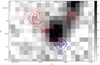 |
Fig. 15 SiO (2–1) integrated intensity over the velocity ranges 3.0– 6.75 km s−1 and 7.0–15.75 km s−1, respectively, in the vicinity of the GCC source 1450 (shown as red and blue contours). The contours levels are 1, 2, and 3 K km s−1 in blue and 2, 3, and 4 Kkm s−1 in red. The background map is the integrated intensity of N2D+, assumed to show the location of the core. The length of the red elongated structure is approximately 0.3 pc. |
5.3.2 The isolated source 1454
The source located in the north clump, 1454, could only be observed with the Effelsberg 100-m telescope in ammonia, which already provides strong indications that it departs from the other sources of the area. It has the highest NH3 column density among the sources (Table D.3). It also has the lowest kinetic temperature and its dust temperature is among the lowest of our sample. It has the highest gas pressure ratio and the lowest α, along with the lowest 12CO, 13CO, and CS peak temperatures, and the highest C18O peak temperature (Figs. B.3 and B.4).
In their Fig. 6 d, Montillaud et al. (2019b) showed that the north clump has lower 12CO excitation temperature (∼14 K) than the rest of the region (∼20–26 K). Since 1454 is part of one of the two filaments colliding at the level of G202, it may be representative of the physical state of the region prior to the collision. As such, it would deserve additional observations to better characterise the evolution of G202 through the collision.
6 Summary
We have examined the G202.3+2.5 region, a clump at the junction of colliding filaments resulting in active star formation at the edge of the Monoceros OB 1 molecular complex. Multiple molecular line observations were analysed to characterise the evolution of the clump and of five of its cores in different phases of star formation. We also analysed a core located approximately 4 pc to the north, which belongs to the same region but is not engaged in the collision process.
We concluded, similarly to other studies, that NH3 in itself is not sufficient to fully characterise dense or moderately dense gas. It is a good intermediate density tracer and when used alongside other density tracers, it can provide a better view of the properties of a region. In this study, it was particularly useful to characterise the evolutionary stage of the cores.
For the six sources, we obtained kinetic temperatures between 10.0 K and 20.4 K, NH3 column densities between 2.5 × 10¹⁴ and 1.9 × 1015 cm−2, and gas pressure ratio values between 0.035 and 0.143, the latter implying the dominance of non-thermal motions in the sources.
For the six cores, we obtained virial parameters in the range 0.002–0.029, implying that the cores are gravitationally unstable. For this calculation we did not take the effect of magnetic field into account, which may contribute to support the cores against infall.
The infall diagnosis based on the comparison of the optically thick HCO+ and optically thin N2H+ lines suggests that the junction region is collapsing in the vicinity of its densest point, about core 1450.
For the five sources of the junction region, N2H+, N2D+, and o-NH2D were detected in all sources.
We found no correlations between N2H+ main beam peak temperature and the parameters from NH3 analysis: NH3 (1,1), FWHM, (1,1), and (2,2) main beam brightness temperatures, kinetic temperature, gas pressure ratio, and virial parameter. This could imply that in our sample NH3 emission is dominated by densities below the threshold for N2H+ to be abundant. The good correlation between the 12CO peak temperature and the NH3 parameters suggests that in our sample NH3 traces more external layers where we detect 12CO.
The NH3 deuterium fractionation values typically between 0.01 and 0.3 are found for our sample with large uncertainties. Similarly to the conclusion of Fontani et al. (2015) and Wienen et al. (2021), we found no correlation between the evolutionary phase of a core and its NH3 deuteration.
The N2H+ deuteration values of our sample distribute between approximately 0.1 and 0.3. They seem to be in line with the conclusion of previous articles that N2H+ deuteration is an evolutionary indicator. Our results confirm that all sources except 1446 are in a young evolutionary stage.
The source 1450, the most massive and the densest among the sources, shows the most deuteration both in NH3 and N2H+, suggesting that it might be close to the onset of gravitational collapse. The N2H+ deuteration and the compact source detected at 100 µm suggest that this source is a young Class 0 object. The nearby linear structure seen in the shock tracer maps of SiO and CH3 OH suggest an outflow from a possible embedded protostar. This interpretation is strengthen by the close-to-bipolar shape of the velocity field in this linear structure. However, based on the Paris-Durham shock models the SiO integrated intensity of this linear structure corresponds to a low velocity shock, which Louvet et al. (2016) interpreted as a sign of converging flows for their studied source. Higher resolution observations would be needed to clarify the nature of this structure.
The source in the northern clump, 1454, based on its NH3, dust, and CO parameters, may represent a physical state of the region before the collision of the filaments. Further studies of the north clump would aid in characterising the evolution of the collision.
Overall, this study strengthened the idea that the junction region arose from the collision or convergence of two filaments. However, it was not possible to draw any conclusions on the origin of this event. In a future study, we will analyse the large scale motions of the gas to investigate the contribution of global collapse and of the expansion of the cavity.
Data availability
Appendices C–F are available on Zenodo.
Acknowledgements
This work is based on observations with the 100-m telescope of the MPIfR (Max-Planck-Institut für Radioastronomie) at Effelsberg and observations carried out under project numbers 113-16 and 151-18 with the IRAM 30-m telescope. IRAM is supported by INSU/CNRS (France), MPG (Germany) and IGN (Spain). The results of this paper are based on an analysis carried out with the CASSIS software and the CDMS and the JPL spectroscopic databases. CASSIS has been developed by IRAP-UPS/CNRS (http://cassis.irap.omp.eu). J.M. and R.B. thank the French ministry of foreign affairs (French embassy in Budapest) and the Hungarian national office for research and innovation (NKFIH) for financial support (Balaton program 40470VL/ 2017-2.2.5-TÉT-FR-2017-00027). R.B. acknowledges support from the French Institute of Hungary, the Carnot-Pasteur Doctoral School of Université de Franche-Comté, and the Physics Doctoral School of Eötvös Loránd University. J.M. thanks the Region Bourgogne Franche-Comté for financial support through the PASCOA project. This work has been achieved in the frame of the EIPHI Graduate school (contract ANR-17-EURE-0002). M.J. acknowledges support from the Research Council of Finland grant No. 348342.
Appendix A Derivation of physical parameters from ammonia data
A.1 Rotational and kinetic temperatures
Rotational temperature between the (1,1) and (2,2) inversion transition can be calculated as outlined by Ho & Townes (1983):
 (A.1)
(A.1)
where τm is the optical depth of the main (1,1) line, T0 = 41.5 K, and TMB is the main beam brightness temperature of the indicated transition.
Excitation temperature of the (1,1) transition can be derived following Harju et al. (1993):
![Mathematical equation: ${T_{{\rm{MB}}}}(1,1) = \eta {{hv} \over k}\left[ {F\left( {{T_{ex}}} \right) - F\left( {{T_{bg}}} \right)} \right]\left( {1 - \exp \left( { - {\tau _{\rm{m}}}(1,1)} \right)} \right),$](/articles/aa/full_html/2025/02/aa48883-23/aa48883-23-eq23.png) (A.2)
(A.2)
where
 (A.3)
(A.3)
Here, η is the beam filling factor, and Tbg is the cosmic background temperature (2.73 K). We used a beam filling factor of 1 for all the calculations we present here, since the emission is extended (Fig. 2).
Kinetic temperature is calculated from the rotational temperature (Tafalla et al. 2004):
 (A.4)
(A.4)
where the energy difference between the (1,1) and (2,2) inversion levels is 41.5 K. In practice we only computed Tkin for S/N values above 4 and 3 for the (2,2) and (1,1) lines, respectively.
A.2 NH3 column density
We derive NH3 column density by calculating the population of the upper or lower energy state of the (J,K)=(1,1) inversion transition first. Assuming a Gaussian line profile for the main line group the population of the upper energy state is taken from
 (A.5)
(A.5)
where ν is the inversion frequency in GHz, Aul is the Einstein A coefficient, ∆υ is the line width, and τm(1,1) is the optical depth of the (1,1) inversion transition (Harju et al. 1993; Fehér et al. 2016). The total column density is then obtained as
 (A.6)
(A.6)
where
 (A.7)
(A.7)
Here, ɡu = 1 and ɡ1 = 1 are the statistical weights of the upper and lower inversion level for the (1,1) inversion transition, respectively.
A.3 Volume density
The H2 volume density can be calculated using the formalism of Harju et al. (1993) and Ho & Townes (1983):
![Mathematical equation: $n\left( {{{\rm{H}}_2}} \right) = {{{A_{{\rm{ul}}}}} \over C}{{F\left( {{T_{{\rm{ex}}}}} \right) - F\left( {{T_{{\rm{bg}}}}} \right)} \over {F\left( {{T_{{\rm{kin}}}}} \right) - F\left( {{T_{{\rm{ex}}}}} \right)}}\left[ {1 + F\left( {{T_{{\rm{kin}}}}} \right)} \right],$](/articles/aa/full_html/2025/02/aa48883-23/aa48883-23-eq29.png) (A.8)
(A.8)
where C is the collisional de-excitation rate (8.5 ×10⁻¹¹ cm3s−1, Danby et al. (1988)), and  .
.
References
- Aikawa, Y., Wakelam, V., Hersant, F., Garrod, R. T., & Herbst, E. 2012, ApJ, 760, 40 [NASA ADS] [CrossRef] [Google Scholar]
- Anathpindika, S. V., & Di Francesco, J. 2022, MNRAS, 513, 1275 [NASA ADS] [CrossRef] [Google Scholar]
- Bergin, E. A., Ciardi, D. R., Lada, C. J., Alves, J., & Lada, E. A. 2001, ApJ, 557, 209 [NASA ADS] [CrossRef] [Google Scholar]
- Bertoldi, F., & McKee, C. F. 1992, ApJ, 395, 140 [NASA ADS] [CrossRef] [Google Scholar]
- Busquet, G., Palau, A., Estalella, R., et al. 2010, A&A, 517, L6 [NASA ADS] [CrossRef] [EDP Sciences] [Google Scholar]
- Cantat-Gaudin, T., Jordi, C., Vallenari, A., et al. 2018, A&A, 618, A93 [NASA ADS] [CrossRef] [EDP Sciences] [Google Scholar]
- Caselli, P. 2002, Planet. Space Sci., 50, 1133 [NASA ADS] [CrossRef] [Google Scholar]
- Caselli, P., Walmsley, C. M., Terzieva, R., & Herbst, E. 1998, ApJ, 499, 234 [Google Scholar]
- Caselli, P., Pineda, J. E., Sipilä, O., et al. 2022, ApJ, 929, 13 [NASA ADS] [CrossRef] [Google Scholar]
- Chevance, M., Kruijssen, J. M. D., Vazquez-Semadeni, E., et al. 2020, Space Sci. Rev., 216, 50 [NASA ADS] [CrossRef] [Google Scholar]
- Crapsi, A., Caselli, P., Walmsley, C. M., et al. 2005, ApJ, 619, 379 [Google Scholar]
- Crapsi, A., Caselli, P., Walmsley, M. C., & Tafalla, M. 2007, A&A, 470, 221 [NASA ADS] [CrossRef] [EDP Sciences] [Google Scholar]
- Dahm, S. E. 2008, in Handbook of Star Forming Regions, Volume I, 4, ed. B. Reipurth, 966 [NASA ADS] [Google Scholar]
- Danby, G., Flower, D. R., Valiron, P., Schilke, P., & Walmsley, C. M. 1988, MNRAS, 235, 229 [NASA ADS] [CrossRef] [Google Scholar]
- Duarte-Cabral, A., Bontemps, S., Motte, F., et al. 2013, A&A, 558, A125 [NASA ADS] [CrossRef] [EDP Sciences] [Google Scholar]
- Emprechtinger, M., Caselli, P., Volgenau, N. H., Stutzki, J., & Wiedner, M. C. 2009, A&A, 493, 89 [NASA ADS] [CrossRef] [EDP Sciences] [Google Scholar]
- Evans, Neal J., I., Heyer, M., Miville-Deschênes, M.-A., Nguyen-Luong, Q., & Merello, M. 2021, ApJ, 920, 126 [NASA ADS] [CrossRef] [Google Scholar]
- Fehér, O., Tóth, L. V., Ward-Thompson, D., et al. 2016, A&A, 590, A75 [Google Scholar]
- Fontani, F., Palau, A., Caselli, P., et al. 2011, A&A, 529, L7 [NASA ADS] [CrossRef] [EDP Sciences] [Google Scholar]
- Fontani, F., Busquet, G., Palau, A., et al. 2015, A&A, 575, A87 [NASA ADS] [CrossRef] [EDP Sciences] [Google Scholar]
- Forbrich, J., Öberg, K., Lada, C. J., et al. 2014, A&A, 568, A27 [NASA ADS] [CrossRef] [EDP Sciences] [Google Scholar]
- Friesen, R. K., Di Francesco, J., Shirley, Y. L., & Myers, P. C. 2009, ApJ, 697, 1457 [Google Scholar]
- Friesen, R. K., Bourke, T. L., Di Francesco, J., Gutermuth, R., & Myers, P. C. 2016, ApJ, 833, 204 [Google Scholar]
- Galloway-Sprietsma, M., Shirley, Y. L., Di Francesco, J., et al. 2022, MNRAS, 515, 5219 [NASA ADS] [CrossRef] [Google Scholar]
- Goldsmith, P. F. 2001, ApJ, 557, 736 [Google Scholar]
- Gómez, G. C., Walsh, C., & Palau, A. 2022, MNRAS, 513, 1244 [CrossRef] [Google Scholar]
- Harju, J., Walmsley, C. M., & Wouterloot, J. G. A. 1993, A&AS, 98, 51 [NASA ADS] [Google Scholar]
- Herbst, E., & van Dishoeck, E. F. 2009, ARA&A, 47, 427 [NASA ADS] [CrossRef] [Google Scholar]
- Ho, P. T. P., & Townes, C. H. 1983, ARA&A, 21, 239 [NASA ADS] [CrossRef] [Google Scholar]
- Jiménez-Serra, I., Caselli, P., Tan, J. C., et al. 2010, MNRAS, 406, 187 [Google Scholar]
- Jørgensen, J. K., Schöier, F. L., & van Dishoeck, E. F. 2004, A&A, 416, 603 [Google Scholar]
- Juvela, M., Ristorcelli, I., Montier, L. A., et al. 2010, A&A, 518, L93 [NASA ADS] [CrossRef] [EDP Sciences] [Google Scholar]
- Juvela, M., Harju, J., Ysard, N., & Lunttila, T. 2012, A&A, 538, A133 [NASA ADS] [CrossRef] [EDP Sciences] [Google Scholar]
- Kauffmann, J., Pillai, T., & Goldsmith, P. F. 2013, ApJ, 779, 185 [NASA ADS] [CrossRef] [Google Scholar]
- Keown, J., Di Francesco, J., Kirk, H., et al. 2017, ApJ, 850, 3 [NASA ADS] [CrossRef] [Google Scholar]
- Krumholz, M. R. 2015, The Formation of Very Massive Stars, 412, ed. J. S. Vink, 43 [NASA ADS] [Google Scholar]
- Kumar, M. S. N., Palmeirim, P., Arzoumanian, D., & Inutsuka, S. I. 2020, A&A, 642, A87 [EDP Sciences] [Google Scholar]
- Lee, C. W., Myers, P. C., & Tafalla, M. 1999, ApJ, 526, 788 [NASA ADS] [CrossRef] [Google Scholar]
- Li, S., Lu, X., Zhang, Q., et al. 2021, ApJ, 912, L7 [NASA ADS] [CrossRef] [Google Scholar]
- Louvet, F., Motte, F., Gusdorf, A., et al. 2016, A&A, 595, A122 [NASA ADS] [CrossRef] [EDP Sciences] [Google Scholar]
- Manjarrez Esquivel, G. 2018, PhD thesis, University of Granada, Spain [Google Scholar]
- Mardones, D., Myers, P. C., Tafalla, M., et al. 1997, ApJ, 489, 719 [Google Scholar]
- Men’shchikov, A., André, P., Didelon, P., et al. 2012, A&A, 542, A81 [Google Scholar]
- Merello, M., Molinari, S., Rygl, K. L. J., et al. 2019, MNRAS, 483, 5355 [NASA ADS] [CrossRef] [Google Scholar]
- Montillaud, J., Juvela, M., Rivera-Ingraham, A., et al. 2015, A&A, 584, A92 [NASA ADS] [CrossRef] [EDP Sciences] [Google Scholar]
- Montillaud, J., Juvela, M., Vastel, C., et al. 2019a, A&A, 631, L1 [NASA ADS] [CrossRef] [EDP Sciences] [Google Scholar]
- Montillaud, J., Juvela, M., Vastel, C., et al. 2019b, A&A, 631, A3 [NASA ADS] [CrossRef] [EDP Sciences] [Google Scholar]
- Motte, F., Bontemps, S., & Louvet, F. 2018, ARA&A, 56, 41 [NASA ADS] [CrossRef] [Google Scholar]
- Naranjo-Romero, R., Vázquez-Semadeni, E., & Loughnane, R. M. 2022, MNRAS, 512, 4715 [NASA ADS] [CrossRef] [Google Scholar]
- Padoan, P., Pan, L., Juvela, M., Haugbølle, T., & Nordlund, Å. 2020, ApJ, 900, 82 [NASA ADS] [CrossRef] [Google Scholar]
- Palau, A., Estalella, R., Girart, J. M., et al. 2007, A&A, 465, 219 [NASA ADS] [CrossRef] [EDP Sciences] [Google Scholar]
- Panessa, M., Seifried, D., Walch, S., et al. 2023, MNRAS, 523, 6138 [NASA ADS] [CrossRef] [Google Scholar]
- Parker, R. J., & Schoettler, C. 2022, MNRAS, 510, 1136 [Google Scholar]
- Pelkonen, V. M., Padoan, P., Haugbølle, T., & Nordlund, Å. 2021, MNRAS, 504, 1219 [NASA ADS] [CrossRef] [Google Scholar]
- Pillai, T., Kauffmann, J., Wyrowski, F., et al. 2011, A&A, 530, A118 [CrossRef] [EDP Sciences] [Google Scholar]
- Rawlings, J. M. C., Taylor, S. D., & Williams, D. A. 2000, MNRAS, 313, 461 [NASA ADS] [CrossRef] [Google Scholar]
- Rawlings, J. M. C., Redman, M. P., Keto, E., & Williams, D. A. 2004, MNRAS, 351, 1054 [Google Scholar]
- Rohlfs, K., & Wilson, T. L. 2004, Tools of radio astronomy (Springer) [Google Scholar]
- Schuller, F., Menten, K. M., Contreras, Y., et al. 2009, A&A, 504, 415 [NASA ADS] [CrossRef] [EDP Sciences] [Google Scholar]
- Sipilä, O., Caselli, P., Redaelli, E., Juvela, M., & Bizzocchi, L. 2019, MNRAS, 487, 1269 [Google Scholar]
- Sokolov, V., Wang, K., Pineda, J. E., et al. 2017, A&A, 606, A133 [NASA ADS] [CrossRef] [EDP Sciences] [Google Scholar]
- Tafalla, M., Myers, P. C., Caselli, P., & Walmsley, C. M. 2004, A&A, 416, 191 [NASA ADS] [CrossRef] [EDP Sciences] [Google Scholar]
- Toth, L. V., & Walmsley, C. M. 1996, A&A, 311, 981 [NASA ADS] [Google Scholar]
- Tóth, L. V., Hotzel, S., Krause, O., et al. 2000, A&A, 364, 769 [NASA ADS] [Google Scholar]
- Tóth, L. V., Haas, M., Lemke, D., Mattila, K., & Onishi, T. 2004, A&A, 420, 533 [NASA ADS] [CrossRef] [EDP Sciences] [Google Scholar]
- Turner, B. E. 1995, ApJ, 449, 635 [NASA ADS] [CrossRef] [Google Scholar]
- Urquhart, J. S., Figura, C. C., Moore, T. J. T., et al. 2015, MNRAS, 452, 4029 [NASA ADS] [CrossRef] [Google Scholar]
- Vastel, C., Bottinelli, S., Caux, E., Glorian, J. M., & Boiziot, M. 2015, in SF2A-2015: Proceedings of the Annual meeting of the French Society of Astronomy and Astrophysics, 313 [Google Scholar]
- Vázquez-Semadeni, E., Palau, A., Ballesteros-Paredes, J., Gómez, G. C., & Zamora-Avilés, M. 2019, MNRAS, 490, 3061 [Google Scholar]
- Walmsley, C. M., Hermsen, W., Henkel, C., Mauersberger, R., & Wilson, T. L. 1987, A&A, 172, 311 [NASA ADS] [Google Scholar]
- Walmsley, C. M., Flower, D. R., & Pineau des Forêts, G. 2004, A&A, 418, 1035 [NASA ADS] [CrossRef] [EDP Sciences] [Google Scholar]
- Watson, W. D. 1977, in Astrophysics and Space Science Library, 70, Topics in Interstellar Matter, eds. H. van Woerden, 135 [CrossRef] [Google Scholar]
- Wienen, M., Wyrowski, F., Schuller, F., et al. 2012, A&A, 544, A146 [NASA ADS] [CrossRef] [EDP Sciences] [Google Scholar]
- Wienen, M., Wyrowski, F., Menten, K. M., et al. 2018, A&A, 609, A125 [NASA ADS] [CrossRef] [EDP Sciences] [Google Scholar]
- Wienen, M., Wyrowski, F., Walmsley, C. M., et al. 2021, A&A, 649, A21 [NASA ADS] [CrossRef] [EDP Sciences] [Google Scholar]
- Yu, N.-P., Xu, J.-L., Wang, J.-J., & Liu, X.-L. 2018, ApJ, 865, 135 [NASA ADS] [CrossRef] [Google Scholar]
- Zucker, C., Speagle, J. S., Schlafly, E. F., et al. 2020, A&A, 633, A51 [NASA ADS] [CrossRef] [EDP Sciences] [Google Scholar]
All Tables
Target properties derived from Herschel observations from the source catalogue (Montillaud et al. 2015).
All Figures
|
Fig. 1 Overview of the morphology and the position of the G202.3+2.5 cloud. Left: schema of the G202.3+2.5 cloud within the context of Mon OB1 East, summarising the results from Paper II. The light gray and light blue areas show the low-density and intermediate-density molecular gas. The five-branch stars mark the positions of the two known open clusters, NGC 2264 and NGC 2259. The four-branch red stars mark the location of groups of protostars. The inward arrows represent the potential global collapse. The outward dashed arrows represent the radiative and mechanical influence exerted by the NGC 2264 open cluster on its surrounding. The insert shows a zoom-in view of the junction region, represented by the hatched area. The triangles mark the location of dense cores. The blue area shows the gas of the filament to the north-east of the junction region. The red area shows the gas of the filament the relates the southern protocluster to the north clump. The directions and red and blue lobes of the two outflows reported in Paper II are also shown. Middle: H2 column density map of the G202.3+2.5 cloud derived from the Herschel/SPIRE data (Montillaud et al. 2015). The lines show the areas of our first IRAM 30-m observations (thin black line; Paper I), of our new IRAM 30-m observations (thick white line), and of our Effelsberg 100-m observations (thick yellow line). Right: zoom-in view of the middle frame with the same colour scale. Black crosses mark the six sources of the GCC catalogue this paper is focussed on. |
| In the text | |
|
Fig. 2 NH3 (1,1) integrated intensity and first moment maps, NH3 (2,2) integrated intensity and kinetic temperature maps, N2H+, HCO+, CH3OH, SiO, N2D+, and o-NH2 D integrated intensity and first moment maps (from top left to bottom right). The white contours on the intensity maps and the black contours on the velocity maps mark N2H+ intensity contours at 1 K km s−1. The black crosses mark the compact sources from the GCC catalogue. The red crosses mark the brightest spots in SiO (northern) and CH3OH (southern). |
| In the text | |
|
Fig. 3 N2H+ integrated intensity map (Montillaud et al. 2019a) with the NH3 spectra of the sources of the deep observations. The colours on the plots of the spectra separate the identified components and their parameters. Red: (1,1) first, stronger component, green: (1,1) second, weaker component, blue: (2,2) first, stronger component, orange: (2,2) second, weaker component. |
| In the text | |
|
Fig. 4 Results of the MC simulations for 1446. Frames a, b and c show parameters obtained for the NH3 (1,1) line, c and d for the (2,2) line. Frames e and f show the distribution obtained for main beam brightness temperature, TMB(1, 1) and TMB(2, 2), g for rotational temperature and h for the NH3 column density. Black crosses mark the values obtained from the CLASS fitting. The black thick dashed lines show the values obtained with the best fit parameter, the black thin dashed lines show the standard deviation, and the red dashed lines indicate the 16th, 50th, and 84th percentiles. |
| In the text | |
|
Fig. 5 NH3 column density vs H2 column density from the GCC catalogue (Montillaud et al. 2015). The dashed lines indicate NH3 abundance values: green dashed line: 2.6 × 10⁻⁸ (Harju et al. 1993, Orion & Cepheus NH3 clumps, median); red dashed line: 7 × 10⁻⁹ (Wienen et al. 2018, ATLASGAL sample, lowest value). The columns of the legend: (1) source name (2) source type: PS: protostellar source, SL: starless source (3) reliability of source classification: 0: unreliable, 1: candidate, 2: reliable. The square marks denote the stronger component, the circle the weaker component of the source. |
| In the text | |
|
Fig. 6 Relationship between temperatures derived from NH3 and dust temperature. Top: NH3 (1,1) main beam temperature as a function of dust temperature (Montillaud et al. 2015). Bottom: kinetic temperature as a function of dust temperature. The red dashed line marks the 1–1 correlation line. The grey line of the least square fit slope is far from 1, two sources with dust temperatures below 10 K have significantly higher kinetic temperatures. The legend is the same as in Fig. 5. |
| In the text | |
|
Fig. 7 Spectra of the observations to the GCC sources 1446 and 1450, and to the coordinates of the brightest SiO and CH3 OH emission, as indicated in the top-right corner of each frame. The red and green vertical lines denote the velocities of the NH3 (1,1) first (stronger) and second (weaker) components, respectively. |
| In the text | |
|
Fig. 8 SiO (2–1) spectra for the three main SiO bright regions (thick grey lines). The red lines show the Gaussian best fit for the SiO spot region, and the skew normal distribution best fit for the other two regions. The insert reproduces the integrated intensity map of SiO shown in Fig. 2. Red contours were added to show the regions where the SiO spectra were considered (SiO spot, 1446–1448, and 1450 bar, from north to south). The grey lines represent the outflow directions from 1446 according to Paper II (their Fig. 12). |
| In the text | |
|
Fig. 9 Correlation between the peak temperatures of SiO (2–1) and CH3OH in the three GCC sources where these transitions were detected. |
| In the text | |
|
Fig. 10 Relationship between shock tracer temperatures and gas pressure ratio. Top: SiO main-beam peak temperature as a function of gas pressure ratio calculated from NH3 line widths. The arrows mark the upper limits of SiO detection of the sources 1451 and 1453. Bottom: CH3OH peak temperature as a function of gas pressure ratio calculated from NH3 [line widths]. The columns of the legend are as in Fig. 5. |
| In the text | |
|
Fig. 11 Correlation between the virial parameter from NH3 data and dust temperature. The symbols are is in Fig. B.3. |
| In the text | |
|
Fig. 12 NH2D/NH3 deuterium fractionation ratio versus NH3 column density. Orange marks denote the dense core sample from a low-mass star forming region of Galloway-Sprietsma et al. (2022), blue marks the low-mass sample from a high-mass protocluster in Li et al. (2021), green marks the pre-protostellar cores of a UCHII region in Busquet et al. (2010), red marks the high-mass ATLASGAL clumps of Wienen et al. (2021), and light blue marks with a black outline denote the NH2D cores (squares) and the NH3 cores (stars) from the pre-protoclusters in Pillai et al. (2011). Our sample is depicted by black crosses, showing the estimates for NH3 column density. The downward arrows mark upper limits for the values depicted. Regarding the sample of Wienen et al. (2021), the rounding of values in the CDS table provided by the authors result in many sources having the exact same values. |
| In the text | |
|
Fig. 13 Parameters from NH3 analysis: (1,1) line width and rotational temperature as a function of NH3 and N2H+ deuterium fractionation. The legend is the same as in Fig. 5. The square marks denote the stronger component, the circle the weaker component of the source. For NH3 deuteration, we see no correlation between the parameters. For N2H+ deuteration, we see a correlation between the evolutionary phase of the sources and the rotational temperature. |
| In the text | |
|
Fig. 14 N2D+ column density versus N2H+ column density. Red symbols denote high mass starless cores (HMSCs), high mass protostellar objects (HMPOs), and ultracompact HII regions (UCHIIs) from Fontani et al. (2011), blue circles denote Class 0 objects from Emprechtinger et al. (2009), and green circles denote low mass starless cores from Crapsi et al. (2005). Our sample is indicated with thick black crosses. The two solid black lines indicate Dfrac values of 0.26 (average Dfrac of the HMSC group) and 0.04 (average Dfrac of the HMPO and UCHII groups), similarly to Fig. 1 of Fontani et al. (2011) to aid comparison. |
| In the text | |
|
Fig. 15 SiO (2–1) integrated intensity over the velocity ranges 3.0– 6.75 km s−1 and 7.0–15.75 km s−1, respectively, in the vicinity of the GCC source 1450 (shown as red and blue contours). The contours levels are 1, 2, and 3 K km s−1 in blue and 2, 3, and 4 Kkm s−1 in red. The background map is the integrated intensity of N2D+, assumed to show the location of the core. The length of the red elongated structure is approximately 0.3 pc. |
| In the text | |
Current usage metrics show cumulative count of Article Views (full-text article views including HTML views, PDF and ePub downloads, according to the available data) and Abstracts Views on Vision4Press platform.
Data correspond to usage on the plateform after 2015. The current usage metrics is available 48-96 hours after online publication and is updated daily on week days.
Initial download of the metrics may take a while.