| Issue |
A&A
Volume 631, November 2019
|
|
|---|---|---|
| Article Number | L1 | |
| Number of page(s) | 20 | |
| Section | Letters to the Editor | |
| DOI | https://doi.org/10.1051/0004-6361/201936377 | |
| Published online | 11 October 2019 | |
Letter to the Editor
Multi-scale analysis of the Monoceros OB 1 star-forming region
I. The dense core population
1
Institut UTINAM – UMR 6213 – CNRS – Univ. Bourgogne Franche Comté, OSU THETA, 41bis avenue de l’Observatoire, 25000 Besançon, France
e-mail: This email address is being protected from spambots. You need JavaScript enabled to view it.
2
Department of Physics, University of Helsinki, PO Box 64 00014 Helsinki, Finland
3
IRAP, Université de Toulouse, CNRS, UPS, CNES, 31400 Toulouse, France
4
Yunnan Observatories, Chinese Academy of Sciences, 396 Yangfangwang, Guandu District, Kunming 650216, PR China
5
Chinese Academy of Sciences, South America Center for Astrophysics (CASSACA), Camino El Observatorio 1515, Las Condes, Santiago, Chile
6
Departamento de Astronomía, Universidad de Chile, Las Condes, Santiago, Chile
7
Shanghai Astronomical Observatory, Chinese Academy of Sciences, 80 Nandan Road, Shanghai 200030, PR China
8
Korea Astronomy and Space Science Institute, 776 Daedeokdaero, Yuseong-gu, Daejeon 34055, Republic of Korea
9
East Asian Observatory, 660 N. A’ohoku Place, Hilo, HI 96720, USA
10
Astrophysics Research Institute, Liverpool John Moores University, IC2, Liverpool Science Park, 146 Brownlow Hill, Liverpool L3 5RF, UK
11
University of Science & Technology, 176 Gajeong-dong, Yuseong-gu, Daejeon, Republic of Korea
12
Academia Sinica, Institute of Astronomy and Astrophysics, Taipei, Taiwan
13
National Astronomical Observatory of Japan, National Institutes of Natural Sciences, 2-21-1 Osawa, Mitaka, Tokyo 181-8588, Japan
14
SOFIA Science Centre, USRA, NASA Ames Research Centre, MS N232-12, Moffett Field, CA 94035, USA
15
Department of Physical Science, Graduate School of Science, Osaka Prefecture University, 1-1 Gakuen-cho, Naka-ku, Sakai, Osaka 599-8531, Japan
16
Department of Physics, School of Science and Humanities, Kabanbay Batyr Ave, 53, Nur-Sultan 010000, Kazakhstan
17
Eötvös Loránd University, Department of Astronomy, Pázmány Péter sétány 1/A, 1117 Budapest, Hungary
18
Department of Earth Science and Astronomy, Graduate School of Arts and Sciences, The University of Tokyo, 3-8-1 Komaba, Meguro, Tokyo 153-8902, Japan
19
Institute of Physics I, University of Cologne, Zülpicher Str. 77, 50937 Cologne, Germany
20
AIM, CEA, CNRS, Université Paris-Saclay, Université Paris Diderot, Sorbonne Paris Cité, 91191 Gif-sur-Yvette, France
21
ICC, University of Barcelona, Marti i Franquès 1, 08028 Barcelona, Spain
22
Konkoly Observatory of the Hungarian Academy of Sciences, Konkoly Thege Miklósút 15-17, 1121 Budapest, Hungary
23
IAPS-INAF, Via Fosso del Cavaliere 100, 00133 Rome, Italy
24
Kavli Institute for Astronomy and Astrophysics, Peking University, 5 Yiheyuan Road, Haidian District, Beijing 100871, PR China
25
European Southern Observatory (ESO) Headquarters, Karl-Schwarzschild-Str. 2, 85748 Garching bei München, Germany
Received:
25
July
2019
Accepted:
9
September
2019
Abstract
Context. Current theories and models attempt to explain star formation globally, from core scales to giant molecular cloud scales. A multi-scale observational characterisation of an entire molecular complex is necessary to constrain them. We investigate star formation in G202.3+2.5, a ∼10 × 3 pc sub-region of the Monoceros OB1 cloud with a complex morphology that harbours interconnected filamentary structures.
Aims. We aim to connect the evolution of cores and filaments in G202.3+2.5 with the global evolution of the cloud and to identify the engines of the cloud dynamics.
Methods. In this first paper, the star formation activity is evaluated by surveying the distributions of dense cores and protostars and their evolutionary state, as characterised using both infrared observations from the Herschel and WISE telescopes and molecular line observations with the IRAM 30 m telescope.
Results. We find ongoing star formation in the whole cloud, with a local peak in star formation activity around the centre of G202.3+2.5, where a chain of massive cores (10 − 50 M⊙) forms a massive ridge (≳150 M⊙). All evolutionary stages from starless cores to Class II protostars are found in G202.3+2.5, including a possibly starless and massive (52 M⊙) core, which presents a high column density (8 × 1022 cm−2).
Conclusions. All the core-scale observables we examined point to an enhanced star formation activity that is centred on the junction between the three main branches of the ramified structure of G202.3+2.5. This suggests that the increased star formation activity results from the convergence of these branches. To further investigate the origin of this enhancement, it is now necessary to extend the analysis to larger scales in order to examine the relationship between cores, filaments, and their environment. We address these points through the analysis of the dynamics of G202.3+2.5 in a joint paper.
Key words: stars: formation / ISM: clouds / dust / extinction
© J. Montillaud et al. 2019
 Open Access article, published by EDP Sciences, under the terms of the Creative Commons Attribution License (http://creativecommons.org/licenses/by/4.0), which permits unrestricted use, distribution, and reproduction in any medium, provided the original work is properly cited.
1. Introduction
Star formation is a key topic in astrophysics that has stimulated the development of many observational programmes and simulation codes. The dramatic increase in computing capabilities over the last decades has made large-scale and high-resolution simulations tractable (e.g. Vázquez-Semadeni et al. 2019; Williams 2018; Sanhueza et al. 2012; Padoan et al. 2017), in contrast to observational projects that are generally more focused on a given scale. Although demanding in observing time, multi-scale observational programmes are now necessary for proper comparison with models. The feasibility and success of such multi-scale observational programmes was demonstrated for example by the ORION B project (Pety et al. 2017; Orkisz et al. 2017, 2019; Gratier et al. 2017) with the IRAM-30 m telescope, the Green Bank ammonia survey (GAS) with the Green Bank Telescope (GBT) 100 m telescope on Gould Belt clouds (Friesen et al. 2017), or the high-resolution study of the infrared dark cloud SDC13 with the Jansky Very Large Array (JVLA) interferometer (Planck Collaboration XI 2011). Increasing the number and diversity of studied star formation regions is a key to improve our understanding of star formation.
We took advantage of the Planck Galactic cold clump catalogue (PGCC; Montier et al. 2010; Poglitsch et al. 2010; Planck Collaboration XIII 2016) and its Herschel follow-up in the frame of the open time key programme Galactic cold cores (GCC; Juvela et al. 2012) to select G202.3+2.5, a nearby filament (760 pc, Montillaud et al. 2015) at the edge of the Monoceros OB1 molecular complex. Its morphology is suggestive of a complex dynamics (Fig. 1), and an intense star formation activity was revealed there by the identification of almost a hundred candidate cold dense cores (Montillaud et al. 2015). Its rich environment includes the young (∼3 Myr) open cluster NGC 2264, an HII region, and a large reservoir of molecular gas. A multi-scale study of this region is needed to shed light on the interplay between the cores, the filaments, and their environment.
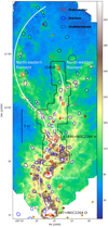 |
Fig. 1. Compact and point source distribution in G202.3+2.5 overlaid on the surface brightness map of PACS 160 μm in MJy sr−1. Red, blue, and black ellipses show GCC sources classified as protostellar, starless, and undetermined. Red four- and six-pointed stars correspond to Class I/II and Class III (or more) YSOs from Marton et al. (2016), respectively. Orange symbols are from Renaud et al. (2013) and circles, four-, and five-pointed stars correspond to Class 0/I, Class II, and transition disks, respectively. The black contour shows the coverage of the IRAM observations. The curved white lines sketch the general structure of the cloud. The white rectangle shows the junction region as represented in Fig. 2. |
In this paper, the first of a series of papers on the Monoceros OB 1 region, we focus on the core scale (∼0.1 pc) and characterise the dense cores in the G202.3+2.5 filaments. We analyse the dust emission in the far-IR (FIR) observed by Herschel and in the mid-IR (MIR) by Wide-Field Infrared Survey Explorer over a 0.5 deg2 area that covers a physical length of approximately 10 pc along the filament. This is combined with the molecular gas emission observed in the millimetre range with the IRAM 30 m telescope. The dynamics at larger scales and its relationship with the core scale are addressed in the next papers of the series.
2. Observations
G202.3+2.5 was mapped with the Herschel instruments Spectral and Photometric Imaging REceiver (SPIRE; Griffin et al. 2010, 250 μm, 350 μm and 500 μm) and Photodetector Array Camera and Spectrometer (PACS; Rapson et al. 2014, 100 μm and 160 μm), as part of the Herschel open time key programme GCC (Juvela et al. 2010). The data were reduced as explained by Juvela et al. (2012). The resolutions are 18, 25, and 37″ (0.07, 0.09, and 0.14 pc) for the 250, 350, and 500 μm bands of SPIRE, and 7.7 and 12″ (0.03 and 0.04 pc) for the 100 and 160 μm bands of PACS. The calibration accuracies of the Herschel SPIRE and PACS surface brightness are expected to be better than 7%1 and 10%2, respectively.
Part of the G202.3+2.5 cloud was observed with the IRAM 30 m telescope during March 2017 at 110 GHz with the Eight mixer receiver (EMIR), targeting the lines of 13CO (J = 1 − 0) and C18O (J = 1 − 0). EMIR was connected to both the versatile spectrometric and polarimetric array (VESPA) and the fast Fourier transform spectrometers (FTS) autocorrelators with spectral resolutions Δν = 20 and 200 kHz (0.055 km s−1 and 0.55 km s−1 at 110 GHz), respectively. The wide passband of the FTS enabled us to also observe 12CO (J = 1 − 0) and N2H+ (J = 1 − 0) lines. Table 1 summarises the observations.
Detected lines in our IRAM observations.
We observed 14 tiles of typically 200″ × 180″, and built a mosaic that covers some 130 arcmin2 around the position  . Each tile was observed multiple times and in orthogonal directions in on-the-fly (OTF) mode and position-switching mode, with a scan velocity of at most 9″ s−1, a dump time of 1 s, and a maximum row spacing of 12″. The beam full width at half-maximum (FWHM) ranges from 21″ (0.08 pc) at 115 GHz to 26″ (0.1 pc) at 93 GHz. The off position was observed every 1 to 1.5 minutes. It was chosen at
  after searching the SPIRE 250 μm map for a minimum in surface brightness. Pointing corrections and focus corrections were performed every 1.5 h and 3 h, respectively, leading to a pointing accuracy measured to be ≲5″. We converted the antenna temperature into the main beam temperature assuming a standard telescope main-beam efficiency3 of 0.78 for CO observations and 0.80 for N2H+.
We also used archival data from the WISE satellite (Wright et al. 2010) at 3.4, 4.6, 12, and 22 μm with a spatial resolution ranging from 6.1″ (0.02 pc) at the shortest wavelength to 12″ (0.04 pc) at 22 μm. We used these data to complement the spectral energy distributions (SEDs) of cores in the MIR range. The data were converted into surface brightness units with the conversion factors given in the explanatory supplement (Cutri et al. 2011). The calibration uncertainty is approximately 6% for the 22 μm band and less for the shorter wavelengths.
3. Method
3.1. Analysis of the molecular line data
For the following analysis, we used multi-component Gaussian fits to characterise the emission lines. For compact sources, spectra in all CO isotopologues were first averaged within the ellipse of the source as defined in the GCC catalogue by Montillaud et al. (2015). A combined single-component Gaussian fit of the 12CO, 13CO, and C18O lines with the same centroid for the three lines was attempted. If the residuals showed features with a signal-to-noise ratio (S/N) greater than five, a new fit with one more component was made, again using the same centroid for all three lines. The residuals were examined again, and new fits with additional components were attempted until the residuals were below 5σ. We found three components at most. Examples for a few sources are shown in Appendix A.1. The constraint that each Gaussian component must have the same centroid in all CO isotopologues was motivated by the following virial analysis, which combines characteristics of two isotopologues. Although the C18O emission is generally weak, it was found to help the fitting procedure significantly to identify reasonable components, especially when two velocity components were not well separated in the spectra of the other isotopologues. Finally, to avoid including extended structures, only components with a significantly peaked radial profile were included (Appendix A.1).
Following the method described by Wilson et al. (2013), we assumed that all CO isotopologues shared the same excitation temperature Tex that was derived from the (assumed) optically thick 12CO (1–0) line. The optical depth of the 13CO and C18O (1–0) lines were then obtained, and their column densities were derived (Appendix A.2). The line widths were used as proposed by MacLaren et al. (1988) to derive the virial parameters by separating the thermal and non-thermal velocity dispersions (Appendix A.3).
3.2. Submillimetre compact sources
To characterise the star formation activity of G202.3+2.5, we investigated the distribution of dense cores and young stellar objects (YSOs) in the cloud, together with their stages of evolution (starless or protostellar). We do not intend to provide an accurate classification (Class I, Class II, etc.) of each embedded YSO, but we used such classification from available public catalogues.
Montillaud et al. (2015) compiled the GCC catalogue, which contains 4466 compact sources extracted from the GCC Herschel maps, including that of G202.3+2.5. They provide the physical characteristics of each source. It includes the mass, dust temperature (Tdust), and the evolutionary stage. Because of the large number of sources and of the variety in their distances, the classification criteria provide good statistical results, but could be optimised for individual clouds.
We here focus on G202.3+2.5, where 98 sources were listed in the GCC catalogue, which enables a more careful examination of individual sources. In Appendix B.2 we present a refinement of the classification method adopted by Montillaud et al. (2015), based on the analysis of the source SED from near-IR (NIR) to FIR wavelengths. We define starless cores as dense sources without protostars, regardless of their ability to eventually form a star, and protostellar cores as dense sources hosting at least one YSO. We also distinguish between candidate protostellar (or starless) sources, for which the proposed evolutionary stage still remains to be confirmed, and reliable protostellar (or starless) sources, when several independent diagnoses lead to the same conclusion (Appendix B.2).
4. Results
Figure 1 shows the distribution of submillimetre compact sources from the GCC catalogue. The range of angular sizes (40–130″) corresponds to approximately 0.15–0.50 pc, implying that each source is likely an individual dense core, although in some cases the better resolution of short-wavelength maps reveals that the source is substructured. Notable examples are (i) the source 1447 in the GCC catalogue where four sources are resolved at 100 μm; (ii) the source 1454 where three sources appear in all PACS and WISE maps; and (iii) source 1457, where two compact sources are resolved in PACS and SPIRE 250 μm maps, one of which is classified as Class 0/I by Renaud et al. (2013).
The blue and red ellipses in Fig. 1 show the starless and protostellar sources, respectively. The individual classification is given in Table D.2. Overall, we obtained 78 starless cores (21 candidates and 57 confirmed cores), 12 protostellar cores (4 candidates and 8 confirmed cores), 1 galaxy, and 7 sources remain unclassified, while in Montillaud et al. (2015) these numbers were 33 (33 and 0), 19 (15 and 4), 0, and 46, respectively. Most differences come from unclassified sources for which our more careful analysis enabled us to propose a classification. Figure 2 shows the example of s1458, where the morphology of the MIR emission reveals that the fluxes measured in WISE bands are not due to a point source associated with the core. Interestingly, this source matches a compact source of N2H+ emission (Fig. 2, left), confirming that s1458 is a genuine starless dense core. The figure also shows s1446, with a typical protostellar SED and a 4.2 ± 0.8 K increase in Tdust. Finally, s1449 is classified as a candidate protostellar source because of its SED, despite a significant decrease in Tdust (−2.1 ± 0.4 K) that is probably due to the envelope of the protostar. We found the latter situation to be widespread and therefore excluded the temperature profiles from the classification scheme (Appendix B.2).
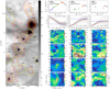 |
Fig. 2. Left: surface brightness map (in MJy sr−1) of PACS 100 μm in the junction region. The colour scale is cut to reveal the cloud structure because the brightest source (s1446) peaks over 60 000 MJy sr−1. The red contours show the integrated emission of N2H+ at 1, 2, 3, 4, and 5 K km s−1. The yellow ellipses show the FWHM of the GCC sources, whose ID numbers are written in black. Right: three columns show for sources 1446, 1449, and 1458 the source SED, its Tdust profile, and maps of WISE 3.4 μm, WISE 12 μm, PACS 100 μm, and SPIRE 250 μm bands. In the SEDs, blue diamonds are 2MASS J, H, and Ks fluxes from the 2MASS PSC. Green upward-pointing triangles are Spitzer 3.6, 4.5, 5.8, 8.0, and 24 μm fluxes from the YSO catalogue of Renaud et al. (2013). Green downward-pointing triangles are WISE 3.4, 4.6, 12, and 22 μm fluxes from our photometry measurements. Orange diamonds are AKARI 9, 18, 65, 90, 140, and 160 μm fluxes from the AKARI MIR and FIR point source catalogues. Red squares show the fluxes of PACS 100 and 160 μm from our photometry measurements. Black circles are fluxes of PACS 160 and SPIRE 250, 350, and 500 μm from the GCC catalogue of compact sources. For the fluxes selected from public point source catalogues, we considered only the source nearest to the GCC source centre. The source number in the GCC catalogue is indicated in the top left corner of the SED plot, as is the final classification (SL = starless, PS = protostellar, 1 = candidate, and 2 = confirmed). In the Tdust profiles, the black points are individual pixels, the blue lines show the background Tdust, the red lines are Gaussian fits, and the grey area shows the 1σ fit uncertainties. |
We computed the virial masses of the 33 GCC sources in the IRAM map from both 13CO and C18O data. The masses M13 and M18 of 13CO and C18O emitting gas, respectively, were also computed using the abundances presented in Appendix A.4. Table D.1 summarises the characteristics of the 26 sources (totalling 35 velocity components) where the peak emission is determined with an S/N > 3 for at least one of the three isotopologues. We computed the virial parameter  , where Mdust is the mass estimate from the GCC catalogue inferred from dust emission. We similarly computed
  . These values should be used carefully because in most cases the line widths of the Gaussian fits are such that σ12 > σ13 > σ18, suggesting that in our sample, optical depth effects often contribute to the line widths and therefore to the virial mass (over-) estimates. In addition, the fact that C18O probes denser layers than 13CO can contribute to differences in line widths. Moreover, when several velocity components are present, Mdust is over-estimated because it includes the emission from all the components.
In our sample, counting each velocity component individually, 15 sources have  . Except for s1461, s1463, s1469, and s1471, all these sources correspond to peaks in N2H+ emission with integrated intensities 1.2 < W < 6.2 K km s−1. Of the 20 unbound sources, only s1459, s1464, and s1472 correspond to a genuine N2H+ emission peak, with W = 1.0, 1.5, 1.4 K km s−1, respectively. Hence, the overall correlation between N2H+ emission and boundedness is very good, as expected considering the N2H+ (1–0) critical density (3 × 105 cm−3, Venuti et al. 2018). Seven of the bound sources are classified as protostellar, six as starless, and the two components of s1450 are undetermined. Of the 20 unbound sources, one is protostellar, 18 are starless, and one is unclassified, which is broadly consistent with a correlation between the source boundedness and its evolutionary stage. The virial parameters
  are generally lower than
  , but the trends remain similar.
5. Discussion: A peak in star formation activity
The star formation activity can be characterised by several tracers. Renaud et al. (2013) classified all the Spitzer sources around NGC 2264 up to the region of the northern filaments of G202.3+2.5. Their Fig. 1 shows that the surface density of protostars decreases from NGC 2264 to G202.3+2.5, and that younger objects (mostly Class 0/I) are found in G202.3+2.5 than in NGC 2264 (mostly Class II). This could support the idea of a gradient and/or a regular time sequence in star formation activity along the south-north direction. Alternatively, the younger sources observed in G202.3+2.5 could be the product of a new episode of star formation in this region.
The distribution of masses from dust observations reported in Table D.1 reveals that six of the nine sources with Mdust > 10 M⊙, including the 52 M⊙ core s1450, where no firm signs of protostellar activity were found, form a chain along the N2H+ bright ridge (Fig. 2) at the junction between the three main filaments of the ramified structure of the cloud (Fig. 1, hereafter “the junction region”). Interestingly, the ridge also hosts the massive protostellar core s1446 (=NGC 2264 H), where Wolf-Chase et al. (2003), using 12CO (2–1) observations, have detected an outflow associated with the nearby Herbig–Haro objects HH 576 and HH 577. We further investigate this outflow in the next paper of this series. Adding only the massive source masses, the ridge is at least 150M⊙. The second most massive source in Table D.1 is s1454 (32 M⊙), where a secondary N2H+ peak is observed (hereafter “the north clump”).
We use our source classification to estimate the star formation activity as a function of declination, a good measure of the distance to the open cluster. Figure 3 shows the variations in the number of sources with declination. The distribution peaks near δ = 10.7°, slightly north of the junction region. The distribution of protostellar sources peaks near δ = 10.6°, at the junction region, where most of the N2H+ bright sources (Fig. 2) are located. The protostellar-to-starless source ratio also peaks in the junction region, and presents a secondary peak at δ = 10.9°, near the north clump.
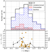 |
Fig. 3. Distributions of submillimetre sources as a function of declination. The blue histogram is for starless cores, the red histogram for protostellar cores, the grey one for sources with undetermined stage of evolution, and the black histogram for all sources. In the lower panel, the black circles show the ratio between the numbers of protostellar and starless cores in each bin, and the orange diamonds show the ratio |

These trends are strengthened by the distribution of the virial parameter  , where 10 out of the 15 bound sources (
 in Fig. 3) are located in the junction region (10.5 ° < δ < 10.7°), 3 are near the north clump (10.8 ° < δ < 11.0°), and the unbound sources are evenly distributed between δ = 10.5° and 10.9°.
Hence, our results strongly suggest a local increase in star formation activity near s1446. This is consistent with the scenario of a new episode of star formation in this region at the northern outskirts of the Mon OB1 complex.
6. Conclusion and perspectives
We have examined the core-scale dust and gas observables in the cloud G202.3+2.5. The evolutionary classification of compact sources was improved compared to Montillaud et al. (2015) to analyse the star formation activity. We have shown that the junction region in G202.3+2.5 is (i) a massive and dense ridge hosting several massive cores, including the active source 1446, responsible for an outflow, and the possibly starless 52 M⊙ core s1450; and (ii) a local peak in the star formation activity of the Mon OB 1 complex. It is striking that this region lies at the junction of three branches of the ramified structure of G202.3+2.5, suggesting that these branches follow a convergent dynamics that has enhanced the star formation activity in the junction region. Determining the origin of this enhancement now requires extending the analysis to larger scales, to examine the relationship between cores, filaments, and their environment. This multi-scale analysis is the focus of the next paper in this series.
The expansion to the third order is accurate to better than 0.1% for Tex > 3 K, and to better than 10−6 for Tex > 12 K.
Acknowledgments
DA acknowledges the funding from Ministry of Education and Science of the Republic of Kazakhstan state-targeted programme BR05236454. DA acknowledges the funding from Nazarbayev University FCDRG110119FD4503 grant support. This work is based on observations carried out under project number 113-16 with the IRAM 30 m telescope. IRAM is supported by INSU/CNRS (France), MPG (Germany), and IGN (Spain). JMo warmly thanks the staff of the 30 m for its kind and efficient help, and in particular Pablo Garcia for stimulating discussions. The project leading to this publication has received funding from the “Soutien à la recherche de l’observatoire” by the OSU THETA. This work was supported by the Programme National “Physique et Chimie du Milieu Interstellaire” (PCMI) of CNRS/INSU with INC/INP co-funded by CEA and CNES. JMo, RB, DC, and VLT thank the French ministry of foreign affairs (French embassy in Budapest) and the Hungarian national office for research and innovation (NKFIH) for financial support (Balaton program 40470VL/ 2017-2.2.5-TÉT-FR-2017-00027). The project leading to this publication has received funding from the European Union’s Horizon 2020 research and innovation programme under grant agreement No 730562 [RadioNet] This research used data from the Second Palomar Observatory Sky Survey (POSS-II), which was made by the California Institute of Technology with funds from the National Science Foundation, the National Geographic Society, the Sloan Foundation, the Samuel Oschin Foundation, and the Eastman Kodak Corporation. MJ and ERM acknowledge the support of the Academy of Finland Grant No. 285769. This research has made use of the SVO Filter Profile Service (http://svo2.cab.inta-csic.es/theory/fps/) supported from the Spanish MINECO through grant AyA2014-55216. J. H. He is supported by the NSF of China under Grant Nos. 11873086 and U1631237, partly by Yunnan province (2017HC018), and also partly by the Chinese Academy of Sciences (CAS) through a grant to the CAS South America Center for Astronomy (CASSACA) in Santiago, Chile. CWL was supported by the Basic Science Research Program through the National Research Foundation of Korea (NRF) funded by the Ministry of Education, Science and Technology (NRF-2019R1A2C1010851). SZ acknowledges the support of NAOJ ALMA Scientific Research Grant Number 2016-03B. KW acknowledges support by the National Key Research and Development Program of China (2017YFA0402702), the National Science Foundation of China (11973013, 11721303), and the starting grant at the Kavli Institute for Astronomy and Astrophysics, Peking University (7101502016). This work has made use of data from the European Space Agency (ESA) mission Gaia (https://www.cosmos.esa.int/gaia), processed by the Gaia Data Processing and Analysis Consortium (DPAC, https://www.cosmos.esa.int/web/gaia/dpac/consortium). Funding for the DPAC has been provided by national institutions, in particular the institutions participating in the Gaia Multilateral Agreement.
References
- Cutri, R. M., Wright, E. L., Conrow, T., et al. 2011, Explanatory Supplement to the WISE Preliminary Data Release Products, Tech. rep. [Google Scholar]
- Endres, C. P., Schlemmer, S., Schilke, P., Stutzki, J., & Müller, H. S. P. 2016, J. Mol. Spectr., 327, 95 [NASA ADS] [CrossRef] [Google Scholar]
- Fehér, O., Juvela, M., Lunttila, T., et al. 2017, A&A, 606, A102 [NASA ADS] [CrossRef] [EDP Sciences] [Google Scholar]
- Friesen, R. K., Pineda, J. E. (co PIs), Rosolowsky, E., et al. 2017, ApJ, 843, 63 [NASA ADS] [CrossRef] [Google Scholar]
- Gaia Collaboration (Prusti, T., et al.) 2016, A&A, 595, A1 [NASA ADS] [CrossRef] [EDP Sciences] [Google Scholar]
- Gratier, P., Bron, E., Gerin, M., et al. 2017, A&A, 599, A100 [NASA ADS] [CrossRef] [EDP Sciences] [Google Scholar]
- Griffin, M. J., Abergel, A., Abreu, A., et al. 2010, A&A, 518, L3 [Google Scholar]
- Juvela, M., Ristorcelli, I., Montier, L. A., et al. 2010, A&A, 518, L93 [NASA ADS] [CrossRef] [EDP Sciences] [Google Scholar]
- Juvela, M., Ristorcelli, I., Pagani, L., et al. 2012, A&A, 541, A12 [NASA ADS] [CrossRef] [EDP Sciences] [Google Scholar]
- MacLaren, I., Richardson, K. M., & Wolfendale, A. W. 1988, ApJ, 333, 821 [NASA ADS] [CrossRef] [Google Scholar]
- Marton, G., Tóth, L. V., Paladini, R., et al. 2016, MNRAS, 458, 3479 [NASA ADS] [CrossRef] [Google Scholar]
- Montier, L. A., Pelkonen, V.-M., Juvela, M., Ristorcelli, I., & Marshall, D. J. 2010, A&A, 522, A83 [NASA ADS] [CrossRef] [EDP Sciences] [Google Scholar]
- Montillaud, J., Juvela, M., Rivera-Ingraham, A., et al. 2015, A&A, 584, A92 [NASA ADS] [CrossRef] [EDP Sciences] [Google Scholar]
- Orkisz, J. H., Pety, J., Gerin, M., et al. 2017, A&A, 599, A99 [NASA ADS] [CrossRef] [EDP Sciences] [Google Scholar]
- Orkisz, J. H., Peretto, N., Pety, J., et al. 2019, A&A, 624, A113 [NASA ADS] [CrossRef] [EDP Sciences] [Google Scholar]
- Padoan, P., Haugbølle, T., Nordlund, A., & Frimann, S. 2017, ApJ, 840, 48 [NASA ADS] [CrossRef] [Google Scholar]
- Pagani, L., Daniel, F., & Dubernet, M.-L. 2009, A&A, 494, 719 [NASA ADS] [CrossRef] [EDP Sciences] [Google Scholar]
- Pety, J., Guzmán, V. V., Orkisz, J. H., et al. 2017, A&A, 599, A98 [NASA ADS] [CrossRef] [EDP Sciences] [Google Scholar]
- Pineda, J. L., Goldsmith, P. F., Chapman, N., et al. 2010, ApJ, 721, 686 [NASA ADS] [CrossRef] [Google Scholar]
- Planck Collaboration XI. 2011, A&A, 536, A23 [NASA ADS] [CrossRef] [EDP Sciences] [Google Scholar]
- Planck Collaboration XIII. 2016, A&A, 594, A28 [NASA ADS] [CrossRef] [EDP Sciences] [Google Scholar]
- Poglitsch, A., Waelkens, C., Geis, N., et al. 2010, A&A, 518, L2 [NASA ADS] [CrossRef] [EDP Sciences] [Google Scholar]
- Rapson, V. A., Pipher, J. L., Gutermuth, R. A., et al. 2014, ApJ, 794, 124 [NASA ADS] [CrossRef] [EDP Sciences] [Google Scholar]
- Renaud, F., Bournaud, F., Emsellem, E., et al. 2013, MNRAS, 436, 1836 [NASA ADS] [CrossRef] [Google Scholar]
- Sanhueza, P., Jackson, J. M., Foster, J. B., et al. 2012, ApJ, 756, 60 [NASA ADS] [CrossRef] [Google Scholar]
- Venuti, L., Prisinzano, L., Sacco, G. G., et al. 2018, A&A, 609, A10 [NASA ADS] [CrossRef] [EDP Sciences] [Google Scholar]
- Vázquez-Semadeni, E., Gómez, G. C., Jappsen, A.-K., Ballesteros-Paredes, J., & Klessen, R. S. 2009, ApJ, 707, 1023 [NASA ADS] [CrossRef] [Google Scholar]
- Vázquez-Semadeni, E., Palau, A., Ballesteros-Paredes, J., Gómez, G. C., & Zamora-Avilés, M. 2019, MNRAS, submitted [arXiv:1903.11247] [Google Scholar]
- Williams, G. M. 2018, PhD Thesis, Cardiff University [Google Scholar]
- Wilson, T. L., & Rood, R. 1994, ARA&A, 32, 191 [NASA ADS] [CrossRef] [Google Scholar]
- Wilson, T. L., Rohlfs, K., & Hüttemeister, S. 2013, Tools of Radio Astronomy (Berlin: Springer Science & Business Media) [CrossRef] [Google Scholar]
- Wolf-Chase, G., Moriarty-Schieven, G., Fich, M., & Barsony, M. 2003, MNRAS, 344, 809 [NASA ADS] [CrossRef] [Google Scholar]
- Wright, E. L., Eisenhardt, P. R. M., Mainzer, A. K., et al. 2010, AJ, 140, 1868 [Google Scholar]
- Zhao, D., Galazutdinov, G. A., Linnartz, H., & Krełowski, J. 2015, A&A, 579, L1 [NASA ADS] [CrossRef] [EDP Sciences] [Google Scholar]
Appendix A: Analysis of molecular lines
A.1. Examples of combined line fitting
As presented in Sect. 3, we performed a combined line fitting of 12CO, 13CO, and C18O data where the same number of velocity components was used for the three lines, and the central velocity of each component was locked between the three transitions. The fitting procedure was semi-automatic, but the small number of sources enabled us to check each fit by eye. Figure A.1 shows a few examples of typical cases with one Gaussian component (s1472), two Gaussian components (s1458), and three Gaussian components (s1521 and s1449).
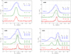 |
Fig. A.1. Examples of combined line fitting with locked velocities for sources s1472, s1458, s1449, and s1521, as indicated in the top left corner of each frame. The best-fit values are also given in the frames in units of km s−1, km s−1, and K for the central velocity vLSR, the velocity dispersion σ, and the peak main-beam temperature Tmb, respectively. |
The radial profiles in integrated intensities W of 12CO, 13CO, and C18O were computed with a running median, and fit by a Gaussian function added to an offset in W. This offset is a measure of the background level. The Gaussian parameters are the maximum integrated intensities Wmax, and the velocity dispersion σ. We kept in the analysis of this paper only sources with a significant Wmax, that is, Wmax/err(Wmax) > 3, where err(Wmax) is the fitting error on Wmax. This enabled us to exclude the components corresponding to extended structures. As an example, Fig. A.2 shows the radial profiles of the three components and three CO isotopologues of s1449. Only the second component corresponds to a significantly peaked profile and is kept in the analysis.
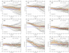 |
Fig. A.2. Radial profiles in CO (top row), 13CO (middle row), and C18O (bottom row) integrated intensities W of the three components (columns) in s1449. Each pixel within a distance of 80″ is shown by a black dot. The running median is shown in orange, with the error bars showing the standard deviation of W in each radius bin. The Gaussian fit to the running median is shown in red, and the offset in blue. The grey area shows the one-sigma uncertainty on the best-fit profiles. The value of the Gaussian amplitude and its uncertainty are shown at the top of each frame. |
A.2. Temperature and density calculations
We calculated the excitation temperatures Tex and column densities of 13CO and C18O following the method described by Wilson et al. (2013). The radiative transfer equation, expressed with the main-beam brightness temperature Tmb, gives
 (A.1)
(A.1)
where T0 = hν/kB (=5.53, 5.26, and 5.25 K for 12CO, 13CO, and C18O, respectively), τν is the optical depth at the frequency ν, and the beam filling factor was taken as 1 because the sources are extended clouds.
When the 12CO (J = 1 − 0) line was optically thick, we derived its excitation temperature:
![Mathematical equation: $$ \begin{aligned} T_{\rm ex} = 5.53 / \ln \left[ 1 + \left( \frac{5.53}{T_{\rm mb}(\mathrm {CO}) + 0.836} \right) \right]. \end{aligned} $$](/articles/aa/full_html/2019/11/aa36377-19/aa36377-19-eq13.gif) (A.2)
(A.2)
In practice, we computed Tex from the brightest channel of Tmb(CO). Because 12CO was observed with FTS200 in parallel to the VESPA observations of 13CO and C18O, it has a coarse resolution of 0.6 km s−1 and therefore an excellent S/N (≳50). Hence, no further smoothing or Gaussian fitting was necessary to derive Tex.
When we assume that 12CO, 13CO, and C18O have the same Tex for the J = 1-0 transition and that this is uniform along the sightline, the optical depth τν of each of the 13CO and C18O J = 1 − 0 lines can be computed by inverting Eq. (A.1). In our data, many pixels exhibit complex line profiles that cannot be fitted by a single Gaussian function. Therefore, instead of classically deriving the column density from the integrated line intensity as in Fehér et al. (2017), for example, we directly integrated τν:
 (A.3)
(A.3)
where we computed the partition function Z(Tex) using the Euler–Maclaurin formula4, the Einstein coefficients were taken from the CDMS database5 (Endres et al. 2016, A10(13CO) = 6.33 × 10⁻⁸ s−1, A10(C18O) = 6.27 × 10⁻⁸ s−1 ), ν10 is the rest frequency of the J = 1 − 0 transition expressed in GHz, and the integral is over the line width in km s−1.
A.3. Virial mass calculation
To estimate the boundedness of sources, we computed the virial mass Mvir of each core mapped with IRAM using the equation by MacLaren et al. (1988):
 (A.4)
(A.4)
where R is the radius of the core, σH2 is the total velocity dispersion of H2, and k = 168 M⊙ pc−1 (km s−1)−2 is a factor that assumes a Gaussian velocity distribution and that the density profile varies as ρ ∝ R−1.5 (MacLaren et al. 1988).
In practice, we computed the effective radius of the cores as the deconvolved geometric average of the semi-major A and semi-minor B axes provided in the GCC catalogue for the opacity map:  , with θ = 38.5″ (Montillaud et al. 2015). The H2 velocity dispersion σH2 was derived from the FWHM line width of a CO isotopologue:
 (A.5)
(A.5)
with σNT the non-thermal velocity dispersion defined as
 (A.6)
(A.6)
where kB is the Boltzmann constant, Tkin is the kinetic temperature, and m and Δv are the mass and the FWHM line width of the CO isotopologue used for the calculation. The latter value was taken for each component of each compact source from the multi-component Gaussian fits presented in Appendix A.1. The calculation was performed for the 13CO and the C18O lines to enable the comparison.
When we assume that local thermal equilibrium (LTE) is satisfied, the kinetic temperature is equal to the excitation temperature Tex. As in Appendix A.2, we used the optically thick 12CO emission to estimate Tex, except that here the value of Tmb(CO) used in Eq. (A.2) is the peak value of the Gaussian fit to the analysed velocity component. As shown by Fehér et al. (2017), the line width fitting uncertainty results in virial mass errors of less than 1%, while optical depth effects in 13CO, considering τ13 ≲ 3, can lead one to overestimate the true FWHM by up to 30% and therefore the virial mass by up to a factor of two. In Sect. 4 we presented the virial analysis for both 13CO and C18O, whose low optical depth alleviates the overestimation problem of 13CO. The distance uncertainty also affects the virial mass linearly, but because we here focused on a single cloud, it acts as a systematic error rather than a random error on the stability analysis.
A.4. Abundances
To estimate the gas mass from CO isotopologue observations, we assumed a ratio XCO/H2 = 1.0 × 10⁻⁴ (e.g. Pineda et al. 2010), and we used the Galactic gradient in C isotopes reported by Wilson & Rood (1994) to compute the ratios X12CO/13CO = 75.9 and X12CO/C18O = 618 for the galactocentric distance of G202.3+2.5 (9.11 kpc, Montillaud et al. 2015).
Appendix B: Source characterisation from IR data
B.1. Spectral energy distributions of GCC sources
To classify and characterise each source, we considered its spectral energy distribution from NIR to FIR wavelengths, as presented in Figs. B.1–B.3. We used the total flux estimates and their associated uncertainties provided for PACS 160 μm and the three SPIRE bands in the GCC catalogue. In addition, we computed the total fluxes and their associated uncertainties for PACS 100 μm, and the four WISE bands at 3.4, 4.6, 12, and 22 μm directly from their maps. To do so, we summed the emission of pixels near the source weighted by a 2D Gaussian defined with the ellipse properties reported for the PACS 160 μm in the GCC catalogue (“AFWHM1”, “BFWHM1”, and “PA1”), and cut at a distance of 3σ from the source centre. We subtracted the background estimated from the median of the pixels in an elliptical annulus between 3.5σ and 5σ from the source centre. The same method applied to the PACS 160 μm map provides results in good agreement with the values in the GCC catalogue, with approximately 55% of sources with relative differences smaller than 30%, and approximately 40% between 30% and 100%. Disagreement typically occurs for sources with complex backgrounds, such as gradients or nearby bright compact sources (e.g. s1488, Fig. C.5).
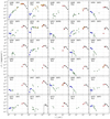 |
Fig. B.1. Spectral energy distributions of GCC sources 1446 to 1475. Blue diamonds are 2MASS J, H, and Ks fluxes from the 2MASS PSC. Green upwards-pointing triangles are Spitzer 3.6, 4.5, 5.8, 8.0, and 24 μm fluxes from the YSO catalogue of Renaud et al. (2013). Green downwards-pointing triangles are WISE 3.4, 4.6, 12, and 22 μm fluxes from our photometry measurements. Orange diamonds are AKARI 9, 18, 65, 90, 140, and 160 μm fluxes from the AKARI MIR and FIR point source catalogues. Red squares show the fluxes of PACS 100 and 160 μm from our photometry measurements. Black circles are fluxes of PACS 160 and SPIRE 250, 350, and 500 μm from the GCC catalogue of compact sources. For the fluxes selected from public point source catalogues, only the source nearest to the GCC source centre was considered. Error bars show the flux uncertainties, but can be smaller than the marker size. The source number in the GCC catalogue is indicated in the top left corner of each frame, along with our evolutionary state classification (SL and PS stand for starless and protostellar, respectively, and the numbers 1 and 2 for candidate and confirmed classification, respectively). The Spitzer-based classification by Renaud et al. (2013) is shown in parentheses. |
We complemented these values with the fluxes found in the 2MASS point source catalogue (PSC, bands J, H, and Ks), the AKARI MIR and FIR PSCs (bands at 9, 18, 65, 90, 140, and 160 μm), and the Spitzer sources reported in the YSO catalogue by Renaud et al. (2013), at 3.6, 4.5, 5.8, 8.0, and 24 μm. For each GCC source, only the nearest source from each of the 2MASS, AKARI, and Spitzer catalogues was considered. In some cases several point sources could be associated with the GCC source, but a single candidate YSO is sufficient to make the GCC source a candidate protostellar core. The YSO catalogue by Renaud et al. (2013) was compiled from cuts in colour-magnitude and colour-colour diagrams. Finally, we also correlated the GCC sources with the YSO catalogue by Marton et al. (2016). This catalogue was built using a support vector machine method on the WISE PSC, leading to an all-sky YSO catalogue. The cross-correlation between this catalogue and the GCC catalogue provides only a few matches, therefore we did not use the fluxes reported in this catalogue.
B.2. Starless versus protostellar: Classification scheme
From the analysis of the SEDs, a first phase of classification of GCC sources was performed as follows. Sources without any associated emission at wavelengths shorter than 100 μm were classified as confirmed starless cores (code 2 in our tables). Sources with an associated MIR source classified as class 0/I or class II by Renaud et al. (2013) were classified as protostellar. In most cases, additional evidence that the core is protostellar could be found, such as the outflows and Herbig–Haro objects associated with s1446 and s1447, or the fact that the compact source is visible at all wavelengths from 3 to 500 μm. The source was then considered a confirmed protostellar core (code 4 in our tables). For s1481 and s1497, no compact emission was detected at 100 μm and the sources were classified as candidate protostellar cores (code 3 in our tables). The Rapson et al. classification of active galactic nuclei (AGNs) and polycyclic aromatic hydrocarbon (PAH) emission was also used to identify six starless cores.
In the second phase, the morphology of the emission in all WISE and Herschel maps for the remaining sources was checked by eye to identify whether it corresponded to a point (or compact) source associated with the core, or to structured background emission. In the latter case, the source was classified as a candidate starless core (code 1 in our tables) when a 2MASS point source was detected, and as a confirmed starless core when no 2MASS emission was found. When MIR compact emission was observed, we searched for evidence that it is (or is not) physically associated with the GCC source. Sources where a large spatial shift (> 80% of the half-width of the GCC source) between the compact MIR and FIR emissions is observed (e.g. s1479) were considered confirmed starless cores. We also searched the Gaia DR2 archive (Gaia Collaboration 2016; Vázquez-Semadeni et al. 2009) for an optical counterpart of the near- and MIR source to compare its parallax with the cloud distance (1.3 mas for a distance of 760 pc). This enabled us to rule out about 40 IR sources whose parallaxes are incompatible with that of the cloud. The corresponding GCC sources (e.g. s1460) were classified as candidate starless cores when 1.3 mas ∉ [π − δπ, π + δπ], where π is the source parallax and δπ its uncertainty, and as confirmed starless cores when 1.3 mas ∉ [π − 3δπ, π + 3δπ]. In two cases (s1451 and s1468), compact emission is visible at all wavelengths from 3 to 500 μm, and we classified the sources as candidate protostellar sources. In the case of s1468, the parallax is compatible with that of the cloud. These two sources were classified as “class III/field star” by Renaud et al. (2013), and might be some of the few genuine class III in this category, which is very likely to be dominated by field stars. For this reason, except for s1451 and s1468, we classified as candidate starless the source where the MIR emission was classified as class III/field star by Renaud et al. (2013). Finally, sources with column densities lower than 2 × 1021 cm−2 were classified as candidate starless cores because this range of densities corresponds to low-density translucent cores rather than dense cores (e.g. Zhao et al. 2015). When cores were classified as candidate starless cores from several independent criteria, we upgraded them to confirmed starless cores.
This scheme enabled us to propose a classification for the 98 GCC sources as summarised in Table D.2. However, it failed to identify a few special cases. We changed the classification of s1509 to extragalactic because of its SED, which peaks at 50 μm, its very low column density (8.4 × 1020 cm−2), and its location, which is very isolated from the filaments. For seven sources, we chose to keep an “undetermined” classification because of contradictory arguments, as summarised in the last column of Table D.2. This is for example the case of s1450, the densest and most massive source in this region, where the Gaia, 2MASS, and MIR detections correspond to a point source that is unlikely to be physically related with the core, but where the compact and relatively strong emission at 100 μm is compatible with a class 0 object. The lack of data near 70 μm makes it difficult to conclude.
In addition, we examined the dust temperature profiles of each source by searching for significant radial increase or decrease in Tdust. From the Tdust map, the pixels within a radius Rmax = 1.5 × AFWHM, where AFWHM is the FWHM of the major axis of the source, were plotted as a function of the distance to the source centre, and the profile was fitted by a 1D Gaussian function. The uncertainty δT on the amplitude ΔT was computed as the standard deviation of the residuals for r < 0.5Rmax. An increase or decrease in Tdust was considered significant where |ΔT|/δT > 3. Table D.2 shows that s1446 is the only protostellar core where the temperature significantly increases towards the centre of the core. For the other protostellar sources, the temperature profile often decreases towards the centre of the core, probably because of the low physical resolution of our Tdust maps at this distance (40″, corresponding to 0.15 pc at 760 pc). Interestingly, the other five sources with a significant Tdust increase towards their centre (s1489, s1499, s1519, s1526, and s1531) have column densities of the order of 2 × 1021 cm−2 and relatively warm temperatures (≳15 K). Most of them also show bright PAH emission at their edges or in their volume. Several other translucent cores show similar MIR morphologies and are tagged as “warm starless” in the last column of Table D.2. We conclude that the Tdust profiles are not a good indication of the starless or protostellar nature of the cores at this distance (and with this resolution), and we do not use them in our classification scheme. The results of this classification are analysed in Sect. 4.
Appendix C: Summary plots of noteworthy sources
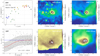 |
Fig. C.1. Same as Fig. 2 for the GCC source 1447, also referred to as IRAS 25 or NGC 2264 O. The cross and plusshow the locations of the 2MASS and Spitzer (as reported by Renaud et al. 2013) point sources, respectively. |
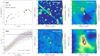 |
Fig. C.3. Same as Fig. C.1 for the GCC source 1454, also referred to as the north clump in this paper. The straight line in the WISE 4.6 μm map is an artefact caused by a bright star ∼7′ to the north-east. |
Appendix D: Additional tables
Fit parameters and virial masses of sources with a peaked emission in 12CO, 13CO or C18O.
Evolutionary state classification of the submillimetre compact sources.
All Tables
Fit parameters and virial masses of sources with a peaked emission in 12CO, 13CO or C18O.
All Figures
|
Fig. 1. Compact and point source distribution in G202.3+2.5 overlaid on the surface brightness map of PACS 160 μm in MJy sr−1. Red, blue, and black ellipses show GCC sources classified as protostellar, starless, and undetermined. Red four- and six-pointed stars correspond to Class I/II and Class III (or more) YSOs from Marton et al. (2016), respectively. Orange symbols are from Renaud et al. (2013) and circles, four-, and five-pointed stars correspond to Class 0/I, Class II, and transition disks, respectively. The black contour shows the coverage of the IRAM observations. The curved white lines sketch the general structure of the cloud. The white rectangle shows the junction region as represented in Fig. 2. |
| In the text | |
|
Fig. 2. Left: surface brightness map (in MJy sr−1) of PACS 100 μm in the junction region. The colour scale is cut to reveal the cloud structure because the brightest source (s1446) peaks over 60 000 MJy sr−1. The red contours show the integrated emission of N2H+ at 1, 2, 3, 4, and 5 K km s−1. The yellow ellipses show the FWHM of the GCC sources, whose ID numbers are written in black. Right: three columns show for sources 1446, 1449, and 1458 the source SED, its Tdust profile, and maps of WISE 3.4 μm, WISE 12 μm, PACS 100 μm, and SPIRE 250 μm bands. In the SEDs, blue diamonds are 2MASS J, H, and Ks fluxes from the 2MASS PSC. Green upward-pointing triangles are Spitzer 3.6, 4.5, 5.8, 8.0, and 24 μm fluxes from the YSO catalogue of Renaud et al. (2013). Green downward-pointing triangles are WISE 3.4, 4.6, 12, and 22 μm fluxes from our photometry measurements. Orange diamonds are AKARI 9, 18, 65, 90, 140, and 160 μm fluxes from the AKARI MIR and FIR point source catalogues. Red squares show the fluxes of PACS 100 and 160 μm from our photometry measurements. Black circles are fluxes of PACS 160 and SPIRE 250, 350, and 500 μm from the GCC catalogue of compact sources. For the fluxes selected from public point source catalogues, we considered only the source nearest to the GCC source centre. The source number in the GCC catalogue is indicated in the top left corner of the SED plot, as is the final classification (SL = starless, PS = protostellar, 1 = candidate, and 2 = confirmed). In the Tdust profiles, the black points are individual pixels, the blue lines show the background Tdust, the red lines are Gaussian fits, and the grey area shows the 1σ fit uncertainties. |
| In the text | |
|
Fig. 3. Distributions of submillimetre sources as a function of declination. The blue histogram is for starless cores, the red histogram for protostellar cores, the grey one for sources with undetermined stage of evolution, and the black histogram for all sources. In the lower panel, the black circles show the ratio between the numbers of protostellar and starless cores in each bin, and the orange diamonds show the ratio |
| In the text | |
|
Fig. A.1. Examples of combined line fitting with locked velocities for sources s1472, s1458, s1449, and s1521, as indicated in the top left corner of each frame. The best-fit values are also given in the frames in units of km s−1, km s−1, and K for the central velocity vLSR, the velocity dispersion σ, and the peak main-beam temperature Tmb, respectively. |
| In the text | |
|
Fig. A.2. Radial profiles in CO (top row), 13CO (middle row), and C18O (bottom row) integrated intensities W of the three components (columns) in s1449. Each pixel within a distance of 80″ is shown by a black dot. The running median is shown in orange, with the error bars showing the standard deviation of W in each radius bin. The Gaussian fit to the running median is shown in red, and the offset in blue. The grey area shows the one-sigma uncertainty on the best-fit profiles. The value of the Gaussian amplitude and its uncertainty are shown at the top of each frame. |
| In the text | |
|
Fig. B.1. Spectral energy distributions of GCC sources 1446 to 1475. Blue diamonds are 2MASS J, H, and Ks fluxes from the 2MASS PSC. Green upwards-pointing triangles are Spitzer 3.6, 4.5, 5.8, 8.0, and 24 μm fluxes from the YSO catalogue of Renaud et al. (2013). Green downwards-pointing triangles are WISE 3.4, 4.6, 12, and 22 μm fluxes from our photometry measurements. Orange diamonds are AKARI 9, 18, 65, 90, 140, and 160 μm fluxes from the AKARI MIR and FIR point source catalogues. Red squares show the fluxes of PACS 100 and 160 μm from our photometry measurements. Black circles are fluxes of PACS 160 and SPIRE 250, 350, and 500 μm from the GCC catalogue of compact sources. For the fluxes selected from public point source catalogues, only the source nearest to the GCC source centre was considered. Error bars show the flux uncertainties, but can be smaller than the marker size. The source number in the GCC catalogue is indicated in the top left corner of each frame, along with our evolutionary state classification (SL and PS stand for starless and protostellar, respectively, and the numbers 1 and 2 for candidate and confirmed classification, respectively). The Spitzer-based classification by Renaud et al. (2013) is shown in parentheses. |
| In the text | |
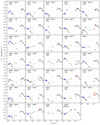 |
Fig. B.2. Same as Fig. B.1 for the GCC sources 1476–1509. |
| In the text | |
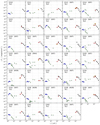 |
Fig. B.3. Same as Fig. B.1 for the GCC sources 1510–1543. |
| In the text | |
|
Fig. C.1. Same as Fig. 2 for the GCC source 1447, also referred to as IRAS 25 or NGC 2264 O. The cross and plusshow the locations of the 2MASS and Spitzer (as reported by Renaud et al. 2013) point sources, respectively. |
| In the text | |
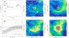 |
Fig. C.2. Same as Fig. C.1 for the GCC source 1452. |
| In the text | |
|
Fig. C.3. Same as Fig. C.1 for the GCC source 1454, also referred to as the north clump in this paper. The straight line in the WISE 4.6 μm map is an artefact caused by a bright star ∼7′ to the north-east. |
| In the text | |
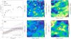 |
Fig. C.4. Same as Fig. C.1 for the GCC source 1457. |
| In the text | |
 |
Fig. C.5. Same as Fig. C.1 for the GCC source 1488. |
| In the text | |
Current usage metrics show cumulative count of Article Views (full-text article views including HTML views, PDF and ePub downloads, according to the available data) and Abstracts Views on Vision4Press platform.
Data correspond to usage on the plateform after 2015. The current usage metrics is available 48-96 hours after online publication and is updated daily on week days.
Initial download of the metrics may take a while.