| Issue |
A&A
Volume 618, October 2018
|
|
|---|---|---|
| Article Number | A46 | |
| Number of page(s) | 22 | |
| Section | Interstellar and circumstellar matter | |
| DOI | https://doi.org/10.1051/0004-6361/201732548 | |
| Published online | 11 October 2018 | |
Core fragmentation and Toomre stability analysis of W3(H2O)
A case study of the IRAM NOEMA large program CORE★,★★
1
Max Planck Institute for Astronomy,
Königstuhl 17,
69117
Heidelberg, Germany
e-mail: This email address is being protected from spambots. You need JavaScript enabled to view it.
2
International Max Planck Research School for Astronomy and Cosmic Physics at the University of Heidelberg (IMPRS-HD)
3
IRAM,
300 Rue de la Piscine, Domaine Universitaire de Grenoble,
38406
St.-Martin-d’Hères, France
4
Institute of Astronomy and Astrophysics, University of Tübingen,
Auf der Morgenstelle 10,
72076
Tübingen, Germany
5
Department of Physics and Astronomy, McMaster University,
1280 Main St. W,
Hamilton,
ON L8S 4M1, Canada
6
I. Physikalisches Institut, Universität zu Köln,
Zülpicher Str. 77,
50937
Köln, Germany
7
Harvard-Smithsonian Center for Astrophysics,
160 Garden St,
Cambridge,
MA 02420, USA
8
INAF, Osservatorio Astrofisico di Arcetri,
Largo E. Fermi 5,
50125
Firenze, Italy
9
Laboratoire d’Astrophysique de Bordeaux – UMR 5804,
CNRS – Université Bordeaux 1, BP 89,
33270
Floirac, France
10
Max-Planck-Institut für Radioastronomie,
Auf dem Hügel 69,
53121
Bonn, Germany
11
Max-Planck-Institut für Extraterrestrische Physik,
Gissenbachstrasse 1,
85748
Garching, Germany
12
Instituto de Radioastronomía y Astrofísica, Universidad Nacional Autonóma de México,
PO Box 3-72,
58090
Morelia,
Michoacan, Mexico
13
School of Physics & Astronomy, E.C. Stoner Building, The University of Leeds,
Leeds
LS2 9JT, UK
14
UK Astronomy Technology Centre, Royal Observatory Edinburgh,
Blackford Hill,
Edinburgh
EH9 3HJ, UK
15
INAF – Osservatorio Astronomico di Cagliari,
Via della Scienza 5,
Selargius
CA 09047, Italy
16
Astrophysics Research Institute, Liverpool John Moores University,
146 Brownlow Hill,
Liverpool
L3 5RF, UK
17
Leiden Observatory, Leiden University,
PO Box 9513,
2300
RA Leiden, The Netherlands
18
CNRS, Institut de Planétologie et d’Astrophysique de Grenoble, Université Grenoble Alpes,
38000
Grenoble, France
19
Max-Planck-Institut für Astrophysik,
Karl-Schwarzschild-Str. 1,
85748
Garching, Germany
20
School of Physics and Astronomy, Cardiff University,
Cardiff
CF24 3AA, UK
21
Centre for Astrophysics and Planetary Science, University of Kent,
Canterbury
CT2 7NH, UK
22
SOFIA Science Center, Deutsches SOFIA Institut, NASA Ames Research Center,
Moffett Field,
CA 94035, USA
23
Universidad Autónoma de Chile,
Av. Pedro de Valdivia 425,
Santiago, Chile
Received:
24
December
2017
Accepted:
21
July
2018
Abstract
Context. The fragmentation mode of high-mass molecular clumps and the properties of the central rotating structures surrounding the most luminous objects have yet to be comprehensively characterised.
Aims. We study the fragmentation and kinematics of the high-mass star-forming region W3(H2O), as part of the IRAM NOrthern Extended Millimeter Array (NOEMA) large programme CORE.
Methods. Using the IRAM NOEMA and the IRAM 30 m telescope, the CORE survey has obtained high-resolution observations of 20 well-known highly luminous star-forming regions in the 1.37 mm wavelength regime in both line and dust continuum emission.
Results. We present the spectral line setup of the CORE survey and a case study for W3(H2O). At ~0.′′35 (700 AU at 2.0 kpc) resolution, the W3(H2O) clump fragments into two cores (west and east), separated by ~2300 AU. Velocity shifts of a few km s−1 are observed in the dense-gas tracer, CH3CN, across both cores, consistent with rotation and perpendicular to the directions of two bipolar outflows, one emanating from each core. The kinematics of the rotating structure about W3(H2O) W shows signs of differential rotation of material, possibly in a disk-like object. The observed rotational signature around W3(H2O) E may be due to a disk-like object, an unresolved binary (or multiple) system, or a combination of both. We fit the emission of CH3CN (12K−11K), K = 4−6 and derive a gas temperature map with a median temperature of ~165 K across W3(H2O). We create a Toomre Q map to study thestability of the rotating structures against gravitational instability. The rotating structures appear to be Toomre unstable close to their outer boundaries, with a possibility of further fragmentation in the differentially rotating core, W3(H2O) W. Rapid cooling in the Toomre unstable regions supports the fragmentation scenario.
Conclusions. Combining millimetre dust continuum and spectral line data toward the famous high-mass star-forming region W3(H2O), we identify core fragmentation on large scales, and indications for possible disk fragmentation on smaller spatial scales.
Key words: stars: formation / stars: massive / stars: early-type / stars: kinematics and dynamics / stars: individual: W3(H2O)/(OH) / techniques: interferometric
Based on observations from an IRAM large program. IRAM is supported by INSU/CNRS (France), MPG (Germany), and IGN (Spain).
Observational data are only available at the CDS via anonymous ftp to cdsarc.u-strasbg.fr (130.79.128.5) or via http://cdsarc.u-strasbg.fr/viz-bin/qcat?J/A+A/618/A46, or alternatively at http://www.mpia.de/core.
© ESO 2018
1 Introduction
Fundamental questions pertaining to the fragmentation of high-mass clumps and the accretion processes that result in the birth of the most massive stars (M ≳ 8 M⊙) still remain unanswered. This is in part due to the clustered nature of star formation and the typically large distances involved. For a long time the existence of high-mass stars had been puzzling as it was thought that the expected intense radiation pressure would prevent the accretion of enough material onto the protostar (e.g. Kahn 1974; Wolfire & Cassinelli 1987). More recently, two- and three-dimensional (magneto)hydrodynamical simulations of collapsing cores have validated the need for accretion disks in the formation of very massive stars, analogous to low-mass star formation (e.g. Yorke & Sonnhalter 2002; Krumholz et al. 2009; Kuiper et al. 2010, 2011; Peters et al. 2010; Kuiper & Yorke 2013; Klassen et al. 2016). Furthermore, different fragmentation processes can contribute to the final stellar mass distribution within a single region, including fragmentation from clouds down to core scales (e.g. Bontemps et al. 2010; Palau et al. 2013, 2015; Beuther et al. 2018; see review by Motte et al. 2018) and disk fragmentation at smaller spatial scales (e.g. Matsumoto & Hanawa 2003; see review by Kratter & Lodato 2016).
In the disk-mediated accretion scenario, the non-isotropic treatment of the radiation field reduces the effect of radiation pressure in the radial direction, such that radiation can escape through the poles along the disk rotation axis, while the disk is shielded due to the high densities. Observationally, the existence of these disks is expected due to ubiquitous observations of collimated outflows (e.g. Beuther et al. 2002; Fallscheer et al. 2009; Leurini et al. 2011; Frank et al. 2014; Maud et al. 2015), which have also been predicted by theoretical models (e.g. Pudritz et al. 2007). Although some accretion disks in differential, Keplerian-like rotation about B-type (proto)stars have been found in recent years (e.g. Carrasco-González et al. 2012; Sánchez-Monge et al. 2013; Beltrán et al. 2014; see reviews by Cesaroni et al. 2007 and Beltrán & de Wit 2016), the existence of such rotating structures around the most massive, O-type protostars is still elusive; only a few cases have been reported to date (Johnston et al. 2015; Ilee et al. 2016; Cesaroni et al. 2017).
As higher resolution observations are becoming more accessible, thus allowing structures to be resolved on scales <1000 AU, it is important to determine whether disks around intermediate to high-mass stars (OB-type) are ubiquitous, and if so, to characterise their properties. What is the typical extent of these disks? Are they in differential rotation about a centrally dominating protostar, similar to their low-mass counterparts, and if so, over what range of radii? Is there any scale where a core stops fragmenting1? At what scales do we see the fragmentation of disks? Are close binary/multiple systems an outcome of disk fragmentation (as suggested by e.g. Meyer et al. 2018)? If so, stability analyses of these high-mass rotating cores and disks are needed to shed light on fragmentation at disk scales. These questions can only be answered with a statistical approach for a large sample of high-mass star-forming regions.
We have undertaken a large programme at IRAM, called CORE (Beuther et al. 2018), making use of the IRAM NOrthern Extended Millimeter Array (NOEMA, formerly Plateau de Bure Interferometer) at 1.37 mm in both line and continuum emission to study the early phases of star formation for a sample of 20 highly luminous (L > 104 L⊙) star-forming regions at high angular resolution (~0.4′′) to analyse their fragmentation and characterise the properties of possible rotating structures. Additionally, observations with the IRAM 30 mtelescope are included to complement the interferometric data, allowing us to understand the role of the environment by studying high-mass star formation at scales larger than those covered by the interferometer. Observations in the 1.3 mm wavelength regime of the CORE project began in June 2014 and finished in January 2017, consisting of a total of more than 400 h of observations with NOEMA. The sample selection criteria and initial results from the observed level of fragmentation in the full sample are presented in Beuther et al. (2018), and details of the 30 m observations and the merging of single-dish observations with interferometric observations can be found in Mottram et al. (2018). In this work, we describe ourspectral setup and present a case study of one of the most promising star-forming clouds in our sample, W3(H2O).
W3(H2O), also known as the Turner–Welch object, resides in the W3 high-mass star-forming region and was initially identified through observations of the dense-gas tracer HCN at 88.6 GHz (Turner & Welch 1984). It is located ~0.05 pc (5′′) east of the well-known ultra compact H II region (UCHII) W3(OH). The name W3(H2O) stems from the existence of water masers in the vicinity of the source (Dreher & Welch 1981), allowing for an accurate distance measurement of 2.0 kpc for this region (Hachisuka et al. 2006; cf. Xu et al. 2006). The relative proper motions of these masers are further explained by an outflow model oriented in the east–west direction (Hachisuka et al. 2006). A continuum source elongated in the east–west direction and spanning the same extent as the water maser outflow has been observed in subarcsecond VLA observations in the radio regime with a spectral index of –0.6, providing evidence for synchrotron emission (Reid et al. 1995; Wilner et al. 1999). This source of synchrotron emission has been characterised by a jet-like model due to its morphology, and the point symmetry of its wiggly bent structure about the centre hints at the possibility of jet precession. Moreover, Shchekinov & Sobolev (2004) attribute this radio emission to a circumstellar jet or wind ionised by the embedded (proto)star at this position. Additional radio continuum sources have been detected in the vicinity of the synchrotron jet, the closest of which is to the west of the elongated structure and has a spectral index of 0.9 (Wilner et al. 1999; Chen et al. 2006), consistent with a circumstellar wind being ionised by another embedded protostellar source. In fact, the high angular resolution (~0.′′7) observations of Wyrowski et al. (1999) in the 1.36 mm band allowed for the detection of three continuum peaks in thermal dust emission, one of which peaks on the position of the water maser outflow and synchrotron jet, and another on the position of the radio continuum source with positive spectral index, confirming the existence of a second source at this position. The detection of two bipolar molecular (CO) outflows further supports the protobinary scenario, suggesting that W3(H2O) may be harbouring at least two rotating structures (Zapata et al. 2011). The two cores within W3(H2O) have individual luminosities on the order of 2 × 10⁴ L⊙, suggesting two 15 M⊙ stars of spectral type B0 (see Sect. 4.3).
In this paper, we study the fragmentation properties of W3(H2O) and the kinematics of the rotating structures within it. We use this source as a test-bed for an expanded study in a forthcoming paper which will focus on the kinematic properties of a larger sample within our survey. The structure of the paper is as follows. Section 2 presents our spectral line setup within the CORE survey with the details of our observations and data reduction for W3(H2O). The observational results are described in Sect. 3. The kinematics, temperature, and stability analysis of W3(H2O) is presented inSect. 4. The main findings are summarised in Sect. 5.
2 Observations and data reduction
2.1 NOEMA observations
Observations of W3(H2O) at 1.37 mm were made between October 2014 and March 2016 in the A-, B-, and D-array configurations of NOEMA in track-sharing mode with W3 IRS4. The compact D-array observations were made with six antennas, while seven antennas were used for the more extended A- and B-array observations. Baselines in the range of 19− 760 m were covered, therefore, the NOEMA observations are not sensitive to structures larger than 12′′ (0.1 pc) at 220 GHz. On-source observations were taken in roughly 20 min increments distributed over an observing run and interleaved with observations of various calibration sources. The phase centre for the observations of W3(H2O) is α(J2000) = 02h 27m03. s87, δ(J2000) = 61°52′24.′′5. A summary of the observations can be found in Table 1.
The full CORE sample of 20 regions has been observed simultaneously with a narrow- and a wide-band correlator. The wide-band correlator, WideX, has four units, each with 1.8 GHz bandwidth, covering two overlapping ranges in frequency inboth horizontal and vertical polarisations (H and V) with a fixed spectral resolution of 1.95 MHz (~2.7 km s−1 at 219 GHz). The full coverage of the WideX correlator is shown in Fig. 1 with bright lines marked. The narrow-band correlator has eight units, each with 80 MHz bandwidth and a spectral resolution of 0.312 MHz (~0.43 km s−1), placed in the 1.37 mm wavelength regime. The frequency coverage of the correlator bands are listed in Table 2. The narrow-band correlator can only process the signal from six antennas; therefore, in cases where the sources were observed with more than six antennas, the correlator automatically accepts the signal from the antennas that yield the best uv-coverage. Important lines covered by the narrow-band receiver are listed in Table 3 and presented in Fig. 2 for the pixel at the phase centre toward W3(H2O).
Data reduction and imaging were performed with the CLIC and MAPPING program of the GILDAS2 software package developed by the IRAM and Observatoire de Grenoble. The continuum was extracted by identifying line-free channels in the range 217 078.6−220 859.5 MHz covered by all four spectral units of the WideX correlator. As we are interested in achieving the highest possible angular resolution, we CLEANed the cubes using the CLARK algorithm (Clark 1980) with a uniform weighting (robust parameter of 0.1)3 yielding a synthesised beam size of 0.′′ 43×0.′′32, PA = 86°, and an rms noise of 3.2 mJy beam−1 for the continuum emission using the combined set of observations in the A-, B-, and D-array configurations (hereafter ABD). We also imaged the data from just the A- and B-array configurations (hereafter AB), as well as the A-array only, for which the synthesised beam sizes and rms noise values are summarised in Table 4.
Continuum subtraction for the lines was performed in the uv-plane by subtracting the emission in the line-free channels in the spectral unit in which the line was observed. Due to line contamination in spectral unit L03, we used the continuum from spectral unit L02 to remove the continuum from spectral unit L03, under the assumption that there is no significant spectral slope between the two adjacent spectral windows. For the WideX continuum subtraction, we subtracted the continuum obtained from line-free channels in all four spectral units. All narrow-band spectra were resampled to a spectral resolution of 0.5 km s−1 and when imaged with the CLARK algorithm and uniform weighting have a negligibly smaller synthesised beam than the continuum images. The average rms noise of the line images in the ABD configuration is 11.2 mJy beam−1 km s−1. The synthesised beam size and the average rms noise of the line data for all imaged combinations of array configurations are listed in Table 4.
Observations of W3(H2O) and W3(OH).
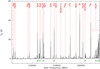 |
Fig. 1 Full WideX spectrum of W3(H2O) averaged over a 4′′ × 4′′ region encompassing two cores, W3(H2O) E and W3(H2O) W, showing the chemical richness of the source. The coverage of the narrow-band correlator units are shown as horizontal green lines and labelled accordingly. The units of the spectrum have been converted from Jy beam−1 to K by multiplying the flux by 188 K Jy−1 under the Rayleigh–Jeans approximation. |
Correlator units and frequency ranges observed with NOEMA.
Bright lines covered in the narrow-band correlator setup.
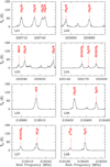 |
Fig. 2 Spectra of the frequency range covered by the narrow-band correlator for the pixel at the phase centre toward W3(H2O). The name of the correlator unit is listed in the bottom left corner of each panel; some of the detected lines are marked. |
Details of CLEANed images.
2.2 IRAM 30 m observations
Observations of W3(H2O) with the 30 m telescope were obtained on March 13, 2015, centred on the same position as the phase centre of the interferometric observations. We used the Eight MIxer Receiver (EMIR) covering the range 213− 236 GHz, reaching a spectral resolution of 0.3 km s−1. In this work, we have merged the NOEMA observations of 13CO with the single-dish observations using the MAPPING software and CLEANed the merged cube with the Steer-Dewdney-Ito (SDI) method (Steer et al. 1984) in order to recover more of the extended features to study molecular outflows. Further details of the 30 m observations and data reduction, as well as the merging process, can be found in Mottram et al. (2018). The resulting merged image has an angular resolution of 1.′′ 14 × 0.′′92, PA = 49°, and an rms noise of 8.4 mJy beam−1 km s−1. We also make use of our single-dish 13CO data which have been reduced and converted to brightness temperatures for a detailed outflow analysis (see Sect. 3.3).
3 Observational results
In the following, we present our detailed analysis for W3(H2O), and when applicable, we also showcase our observational results for W3(OH). Our analysis mainly uses the continuum and CH 3CN spectral line emission. Maps of the other lines are shown in Appendix A.
3.1 Continuum emission
Figure 3 shows the 1.37 mm (219 GHz) continuum emission map of W3(H2O) and W3(OH) in the ABD configuration. At this wavelength, the continuum emission in our field of view is dominated in W3(OH) by free–free emission, while the emission in W3(H2O) is due to dust (Wyrowski et al. 1999). In the following, we focus on the fragmentation and kinematics of the younger region, W3(H2O).
Figure 4 shows a comparison of the continuum emission maps of W3(H2O) obtained by imaging the ABD, AB, and A-array only observations. The integrated flux within the 6σ contours is 1220, 656, and 364 mJy for the ABD, AB, and A-array images, respectively. The fragmentation of W3(H2O) into two cores, separated by ~2300 AU, is best seen in the AB image at 700 AU scales. The two cores are labelled W3(H2O) E and W3(H2O) W, and their peak continuum positions are depicted by stars in Fig. 4, marking the positions of embedded (proto)stars. The peak position of W3(H2O) E is α(J2000) = 02h 27m04. s73, δ(J2000) = 61°52′24.′′66, and that of W3(H2O) W is α(J2000) = 02h27m04. s57, δ(J2000) = 61°52′24.′′59. The approximate separation boundary between W3(H2O) E and W is marked with a vertical dashed line. The integrated flux within 6σ contours and the separation boundary are 377 and 279 mJy for W3(H2O) E and W3(H2O) W, respectively. Furthermore, there is an additional emission peak to the northwest of W3(H2O) at an offset of −1.′′6, 1.′′ 6 (α(J2000) = 02h 27m04. s37, δ(J2000) = 61°52′26.′′35), which is best seen in the ABD image as it has the best sensitivity. This is most likely a site for the formation of lower mass stars.
Radiative transfer models by Chen et al. (2006) for W3(H2O) in the 1.4 mm wavelength regime show that the averaged dust optical depth is less than 0.09; therefore, we assume the thermal dust emission to be optically thin in our observations. The positions of continuum peaks A and C from Wyrowski et al. (1999) coincide well with the continuum peaks W3(H2O) E and W3(H2O) W in our observations to within a synthesised beam (see Fig. 4). Wyrowski et al. (1999) had attributed the third peak in their observations between the other two cores to an interplay of high column density and low temperatures in the central region, and concluded that W3(H2O) is harbouring two cores at the positions of continuum peaks A and C. Our double-peaked continuum image in AB, with a better spatial resolution than that of Wyrowski et al. (1999) by a factor of 3.3, supports this interpretation. Furthermore, peak B coincides well with the northeast extension of W3(H2O) W in our observations, best seen in the middle panel of Fig. 4.
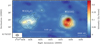 |
Fig. 3 NOEMA 1.37 mm (219 GHz) continuum image toward W3(H2O) and W3(OH) in the ABD configuration. The solid contours start at 6σ and increase in steps of 6σ (1σ = 3.2 mJy beam−1). The dotted contours show the same negative levels. A scale bar and the synthesised beam (0.′′ 43×0.′′32, PA = 86°) are shown at the bottom. |
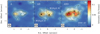 |
Fig. 4 1.37 mm continuum image toward W3(H2O) observed with the A (left panel), AB (middle panel), and ABD (right panel) configurations of NOEMA. The solid contours start at 6σ and increase in steps of 3σ (see Table 4). Synthesised beams are shown in the bottom left corners of each panel, along witha scale bar in the bottom right of the right-hand panel. The black stars in the middle panel correspondto the positions of the continuum peaks, marking the locations of the two individual cores, W3(H2O) W and W3(H2O) E, with the dashed line as the approximate separation boundary. The white stars in the right panel correspond to the positions of the continuum peaks A, B, and C from Wyrowski et al. (1999). The offset zero position is the phase centre of the observations: α(J2000) = 02h 27m03. s87, δ(J2000) = 61°52′24.′′5. |
3.2 Line emission
W3(H2O) is one of the most chemically rich sources in our sample (see Fig. 1) with detections of sulphur-bearing species such as 33SO and 34SO2, complex species such as HCOOCH3, and vibrationally excited linesof HC3N, among many others. Figure 5 shows integrated intensity (zeroth moment) and intensity-weighted peak velocity (first moment) maps of CH3CN (123−113) for W3(H2O) and W3(OH). The zeroth moment map confirms the fragmentation of W3(H2O) into two cores. The moment maps of most lines covered by the narrow-band receiver (see Table 3 and Fig. 2) are presented in Appendix A. All moment maps have been created inside regions where the signal-to-noise ratio (S/N) is greater than 5σ. The integrated intensity maps of most tracers for W3(H2O) also show two peaks coincident with the locations of W3(H2O) E and W3(H2O) W. While the continuum emission is stronger for W3(H2O) E, some dense gas tracers (e.g. CH3CN, HC3N) show stronger line emission towards W3(H2O) W.
The bottom panels in Fig. 5 show the intensity-weighted peak velocity (first moment) map of the region in CH 3CN (123−113). We chose to do our kinematic analyses on this transition as it is the strongest unblended line in the methyl cyanide (CH 3CN) K-ladder. There is a clear velocity gradient in the east–west direction across W3(H2O), and in the NW–SE direction across W3(OH). The systemic velocities of both clumps are determined by averaging the spectra of CH 3CN (123−113) over a 4′′ × 4′′ area centred on each source and fitting a Gaussian line to the resulting averaged spectrum. In this way, W3(H2O) and W3(OH) have average velocities of –49.1 and –45.0 km s−1, respectively.
The velocity gradient across W3(H2O) is detected in most of the high spectral resolution lines in our survey (see Fig. A.2) and spans ~6000 AU in size, corresponding to an amplitude of 170 km s−1 pc−1. The velocity gradient resolved in W3(OH) has an amplitude of ~100 km s−1 pc−1 and is roughly perpendicular to the motion of the ionised gas in the east–west direction as traced by the H92α line in observations of Keto et al. (1995), and is perpendicular to the direction of the “champagne flow” observed to the northeast at radio frequencies (Keto et al. 1995; Wilner et al. 1999). Thus, in W3(OH) we seem to be witnessing the large-scale motion of the remnant molecular gas. The interpretation of line emission for W3(OH) is complex because most of the continuum emission at 1.37 mm is due to free–free emission which affects the appearance of molecular lines. In practice, free–free emission at 1.3 mm reduces the molecular line emission which is reflected by the reduced integrated line emission towards the peaks of W3(OH). As this is beyond the scope of this paper, we refrain from further analysis of W3(OH).
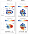 |
Fig. 5 Top row: integrated intensity (zeroth moment) map of CH3CN (123−113) for W3(H2O) (left panel) and W3(OH) (right panel) in the ABD configuration. Bottom row: intensity-weighted peak velocity (first moment) map of CH3CN (123−113) for W3(H2O) (left panel) and W3(OH) (right panel) in the ABD configuration. The dashed line corresponds to the cut made for the PV plot of W3(H2O) presented in Fig. 8. The solid contours correspond to the 1.37 mm continuum, starting at 6σ and increasing in steps of 6σ (1σ = 3.2 mJy beam−1). The dotted contours correspond to the same negative levels. A scale bar and the synthesised beam (0.′′ 43×0.′′32, PA = 86°) are shown in the top right panel. |
3.3 Outflow structure
In Fig. 6, we show integrated intensity (zeroth moment) maps of outflow-tracing molecules (12 CO and 13CO) for the redshifted and blueshifted gas. The minimum intensity below which a pixel is not considered in the creation of the moment maps is based on 5σ rms noise level in emission-free channels. The single-dish CO (2–1) map (see top left panel of Fig. 6) shows the existence of a bipolar outflow in the overall vicinity of W3(H2O) but also encompassing W3(OH) in an approximately NE–SW direction. The 13CO (2–1) single-dish map (see top right panel of Fig. 6) shows less extended emission than the 12CO as the 13C isotopologue is a factor of ~76 less abundant (Henkel et al. 1982), and the map highlights the general NE–SW direction of the outflow even better.
The integrated intensity map of 12CO from SMA interferometric data of Zapata et al. (2011) allows for the detection of two bipolar outflows (see bottom left panel of Fig. 6). The outflow emanating from W3(H2O) E has its blueshifted side to the southwest and its redshifted lobe to the northeast, while the second outflow emanating from W3(H2O) W has its blueshifted side extending to the northeast with its redshifted side to the southwest (Zapata et al. 2011). The difference between the position angles of the two outflows (in the plane of the sky) is 25°. Furthermore, the resulting zeroth moment map of 13CO emission from our combined NOEMA and 30 m single-dish observations, presented in the bottom right panel of Fig. 6, confirms thefindings of Zapata et al. (2011) with regards to the directions and origin of the redshifted outflow lobe from W3(H2O) W and the origins of the blueshifted outflow lobe from W3(H2O) E. However, we miss much of the emission that is detected in the 12CO SMA interferometric data, mainly due to the lower abundance of the 13C isotopologue, and thus its lower sensitivity to the outflowing gas. The same coloured arrows obtained from Zapata et al. (2011) are redrawn in a zoom panel inside the bottom right panel of this figure, highlighting that the two outflows are in fact emanating from different positions.
In Fig. 7, we show how the centimetre emission aligns with the millimetre continuum emission. The directions of bipolar molecular outflows emanating from the cores are shown by red and blue arrows, and the positions of water masers shown by yellow triangles. The elongated radio source centred on W3(H2O) E has a spectral index of –0.6 and is a source of synchrotron emission, best described by a jet-like model due to its morphology (Reid et al. 1995; Wilner et al. 1999). The radio source centred on W3(H2O) W, however, has a rising spectral index, possibly due to a circumstellar wind being ionised by an embedded (proto)stellar source at this position. Furthermore, the discrepancy between the direction of the synchrotron jet-like object and the molecular outflow could be due to the existence of multiple objects in this core, unresolved by our observations. Interestingly, it has been shown that synchrotron radiation can be produced not only via jets, but also through the acceleration of relativistic electrons in the interaction of disk material with a stellar wind (Shchekinov & Sobolev 2004), providing an alternative explanation for the maser and cm emission.
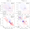 |
Fig. 6 Top left panel: intensity map of CO (2–1) emission from IRAM 30 m integrated over the velocity range from − 40 to − 20 km s−1 for the redshifted and from − 80 to − 55 km s−1 for the blueshifted gas. Contours start at 5σ and increase in steps of 5σ (1σ = 1.9 K km s−1). Top right panel: intensity map of 13CO (2–1) emission from IRAM 30 m integrated over the velocity range from − 40 to − 20 km s−1 for the redshifted and from − 80 to − 55 km s−1 for the blueshifted gas. Contours start at 3σ and increase in steps of 2σ (1σ = 0.42 K km s−1). Bottom left panel: intensity map of CO (2–1) emission obtained by Zapata et al. (2011) with the SMA integrated over the velocity range from − 45 to − 25 for the redshifted and from − 75 to − 55 for the blueshifted gas. Contours start at 5σ and increase in steps of 5σ (1σ = 1.1 mJy beam−1 km s−1). The blue and red arrows highlight the positions and directions of the CO outflows emanating from each source. Bottom right panel: intensity map of 13CO (2–1) emission from IRAM 30 m merged with NOEMA observations integrated over the velocity range from − 41 to − 30 for the redshifted and from − 70 to − 53 for the blueshifted gas. Contours start at 3σ and increase in steps of 3σ (1σ = 0.03 mJy beam−1 km s−1 for redshifted and 0.17 mJy beam−1 km s−1 for blueshifted sides). The zoom panel in the top left corner highlights the launching positions of each outflow, with the red and blue arrows showing the directions of the two bipolar outflows from Zapata et al. (2011). The rms noise used in drawing the contours of the integrated intensity maps have been determined by first creating the maps without any constraints on the minimum emission level (threshold of 0) and calculating the noise in an emission-free part of the resulting map. |
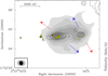 |
Fig. 7 NOEMA 1.37 mm (219 GHz) continuum image toward W3(H2O) in grey with levels starting at 6σ and increasing in steps of 6σ. The black contours correspond to the cm emission from Wilner et al. (1999). The positions of H2O masers obtained from Hachisuka et al. (2006) are plotted as yellow triangles. The blue and red arrows show the directions of bipolar molecular outflows from Zapata et al. (2011; see Fig. 6). The synthesised beam size of the cm emission (0.′′ 21×0.′′19, PA = 68°) is shown in black in the bottom left corner. The synthesised beam size of our mm continuum image is shown in grey in the bottom left corner. |
4 Analysis and discussion
4.1 Dense gas kinematics
The kinematics of W3(H2O) can be further analysed by looking at position–velocity (PV) diagrams for various transitions of dense gas and potentially disk-tracing molecules such as CH3CN and HCOOCH3 (e.g. Beuther et al. 2005). In the following, we divide our focus between the large-scale kinematics of the entire W3(H2O) region, where we put forward arguments for the observed velocity gradients in CH 3CN and HCOOCH3 being due to rotation instead of infall (Sect. 4.1.1), and the small-scale kinematics of the two separate cores within W3(H2O) (Sect. 4.1.2). Although the alignment of the elongated radio emission with the water masers can be described by an outflow model oriented in the east–west direction, the detection of two molecular outflows emanating from the positions of the two continuum peaks, roughly perpendicular to the observed velocity gradient in CH 3CN at large scale and perpendicular to the observed velocity gradients on smaller scales (see Sect. 4.1.2), make it unlikely that the motions in CH 3CN would be due to expansion or outflow. Furthermore, CH3CN and HCOOCH3 line profiles do not show the broad components typically seen in emission from expanding gas, and these species are nevertheless too complex to exist in an ionised jet. We, therefore, conclude that the observed velocity gradient is most likely due to rotation, which we will assume for the remainder of this paper.
4.1.1 Large-scale kinematics
The PV plots of CH3CN and HCOOCH3 for W3(H2O) are shown in Fig. 8 for a cut in the direction of the velocity gradient going through the continuum peaks (dashed line in bottom left panel of Fig. 5) obtained from the NOEMA observations. The white curves in the top left panel correspond to gas in Keplerian rotation with V rot ∝ R−1∕2 about a 10, 25, and 50 M⊙ central object. These white curves are not fits to the PV diagram, but are merely drawn to guide the eye. It is clear that the gasis not in Keplerian rotation; however, higher velocity gas is observed closer to the centre of W3(H2O) which can be a signpost for differential rotation.
Ohashi et al. (1997) created models for comparison to their interferometric data of the low-mass protostar L1527, using a thin disk with 2000 AU extent configured edge-on and present PV diagrams for cases with various degrees of infall and rotation. In the case of infall-only motions, their PV plots are axisymmetric with two peaks offset symmetrically in the velocity axis. With the addition of rotation, the peaks become blueshifted and redshifted away from the central positions such that in the case of a pure Keplerian rotation and in the absence of infall we would recover the classical butterfly-shaped rotation curve. Comparing our PV plots to the Ohashi et al. (1997) scenarios, we observe minimal contributions in the top left and bottom right quadrants of our plots where one would expect some emission in the cases including infall motions. Therefore, we do not detect infall motions in our interferometric data probably because the infalling envelope is too diffuse and filtered out. Furthermore, models by Tobin et al. (2012) for spherical rotating collapse and filamentary rotating collapse showed similar results to that of Ohashi et al. (1997), confirming that the absence of infall results in the lack of emission in those quadrants and not the projection or source morphology. Moreover, the PV plots of HCOOCH3, which is a less abundant species than CH3CN, are more representative of rigid body-like rotation.
Chen et al. (2006) generated a binary model with radiative transfer post-processing of methyl cyanide for each source within W3(H2O), showing that the high-velocity deviations from solid body rotation in their PV plots could be a result of two spatially unresolved cores (on similar scales to our observations) with a small radial velocity difference. The detection of a smooth velocity gradient in all tracers across W3(H2O) E and W suggests that the observed angular velocity difference cannot be solely due to binary motion of the cores, but that there is also a large-scale toroidal structure encompassing and rotating about the two resolved cores. Such circumbinary toroidal structures have indeed been observed previously at lower angular resolutions in other sources (e.g. Beltrán et al. 2005; Beuther et al. 2007).
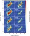 |
Fig. 8 Position–velocity plots of W3(H2O) for a cut in the direction of rotation as depicted by a dashed line in the bottom left panel of Fig. 5 for various species and transitions in the ABD configuration. The vertical dashed lines correspond to the centre of the cut. The vertical dotted lines correspond to the positions of continuum peaks corresponding to W3(H2O) E and W3(H2O) W. The horizontal dashed lines correspond to the LSR velocity of W3(H2O). The black contours start at 4σ and increase in steps of 6σ. The white solid, dashed, and dotted lines in the top left panel correspond to the region within which emission is expected if the gas is in a disk in Keplerian rotation about a 10, 25, 50 M⊙ star, respectively.The white curves are not fits to the rotation curve, but are drawn to guide the eye. A scale bar and a cross that corresponds to the spatial and spectral resolutions are shown in the bottom right panel. |
4.1.2 Small-scale kinematics
Although we see a smooth velocity gradient in CH3CN across the entire W3(H2O) structure, the existence of at least two cores within it as presented by our continuum results, and two collimated outflows requires further analysis. Imaging the data in the most extended configuration and therefore reaching our highest resolution, we can filter out the large-scale envelope to analyse the kinematics of gas around each of the cores. Figure 9 shows the first moment map of CH 3CN (123−113) for the cores to the east and west using the A-array observations exclusively. The maps have been scaled and masked to highlight the velocity structure of each core. The mean line-of-sight velocity difference between the two main cores, W3(H2O) W and E, is a few km s−1. Velocity differences of a few km s−1 are observed across each core, approximately perpendicular to the directions of the bipolar molecular outflows emanating from each core (Zapata et al. 2011). This indicates that the small-scale gradients across each individual core are most likely due to rotation. The two line-of-sight velocity gradients are on the order of ~1000 km s−1 pc−1, depending on the choice for the extent of the gradient, much faster than the rotational motion of 170 km s−1 pc−1 for the whole of W3(H2O) from the ABD data. Furthermore, the directions of the velocity gradients observed for each core are slightly inclined with respect to the overall east–west motion of the gas on larger scales (Fig. 5), suggesting that the general rotation seen around the two cores may be inherited from the large-scale rotation. Meanwhile, the direction of the blueshifted (redshifted) outflow emanating from W3(H2O) W is almost inthe opposite direction of the blueshifted (redshifted) outflow ejected from W3(H2O) E. This impliesthat the inclination angles of the two rotating structures with respect to the plane of the sky are likely different.
Figure 10 shows PV diagrams for W3(H2O) E (left) and W3(H2O) W (right) corresponding to cuts in the directions of rotation as depicted by dashed lines in Fig. 9. Based on the PV plots, the LSR velocities of W3(H2O) E and W3(H2O) W are estimated tobe −51 and −47 km s−1, respectively.White curves correspond to gas in Keplerian rotation about a 5, 10, and 15 M⊙ centrally dominated object. As on larger scales, these PV diagrams do not show the symmetric four-quadrant shape expected if the velocity gradients were due to infall.
The PV plot for W3(H2O) W contains contributions from W3(H2O) E due to the angle and extent of the cut, hence there is added emission in quadrants toward positive offset, making it difficult to infer rotational signatures pertaining to the blueshifted emission of W3(H2O) W. The redshifted rotational signatures seen in the quadrants toward negative offsets, however, show signatures of increased gas velocities closer to thecentre of the core. Such a trend in the PV plot implies differential rotation of material, possibly within a disk-like object.
Position–velocity plots for W3(H2O) E have a lower S/N than W3(H2O) W as line emission is typically weaker for this fragment even though its 1.37 mm dust continuum peak is stronger. The linearity of the rotation curves in CH3CN does not reveal Keplerian signatures, but is more consistent with rigid body-like rotation. In order to increase the S/N, we stacked the PV plots of CH3CN (12K−11K), K = 2−5 and show this stacked PV plot in the bottom right panel of Fig. 10 for W3(H2O) E. Stacking is a reasonable strategy as the variation in average linewidths of these transitions around this core is below our spectral resolution; therefore, assuming these lines to be probing the same surface is valid. In the stacked image, the 4σ contour reveals a high-velocity feature close to the centre of the core toward positive offsets. As this feature has an extent of the order of our spatial resolution, it is unclear whether the rotation observed for W3(H2O) E is due to a disk-like object, an unresolved binary (or multiple) system, or a combination of the two.
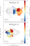 |
Fig. 9 Intensity-weighted peak velocity (first moment) map of CH3CN (123−113) using only the A-array observations and masked out to show contributions from W3(H2O) W (top panel) and W3(H2O) E (bottom panel). The solid contours correspond to the 1.37 mm continuum in the A-array only observations and start at 6σ and increase in steps of 3σ (1σ = 2.5 mJy beam−1). The dashedlines correspond to the cuts made for the PV plots (Fig. 10). The blue and red arrows show the directions of bipolar molecular outflows (Fig. 6). A scale bar and the synthesised beam (0.′′ 39×0.′′28, PA = 88°) are shown in the bottom. The velocity ranges are different for the two cores. |
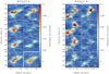 |
Fig. 10 Position–velocity plots along a cut in the direction of rotation as depicted by dashed lines in Fig. 9 for a fragment to the east (left panel) and to the west (right panel). The black contours start at 4σ and increase in steps of 6σ. The white solid, dashed, and dotted lines correspond to the region within which emission is expected if the gas is in a disk in Keplerian rotation about a 5, 10, and 15 M⊙ star, respectively. The crosses in the bottom right corners correspond to the spatial and spectral resolutions. Regions to the left of the dotted vertical line in the right figure contain contributions from W3(H2O) E. |
4.2 Temperature distribution
As a symmetric top molecule, CH3CN is an excellent thermometer of hot molecular gas (e.g. Loren & Mundy 1984; Zhang et al. 1998) since its relative populations in different K-levels are dominated by collisions. Our high spectral resolution observations of CH 3CN covers its J = 12−11, K = 0−6 transitions and some of their isotopologues which have upper energy levels in the range 70–325 K with 0.5 km s−1 spectral resolution (see Table 3).
We made use of the eXtended CASA Line Analysis Software Suite (XCLASS4; Möller et al. 2017)to model the observed spectra under the assumption of Local Thermodynamical Equilibrium (LTE), which is typically valid for CH3CN in such high-densityenvironments (see Sect. 4.3). In summary, XCLASS solves the radiative transfer equation in one dimension for a set of initial conditions (source size, column density, temperature, linewidth, and peak velocity) provided by the user, and through a χ2 minimisation routine changes the initial conditions within ranges that have been provided by the user to obtain the best fit to the observed spectra. The details of our XCLASS modelling are summarised in Appendix B.
In Fig. 11, we present our results of pixel-by-pixel XCLASS modelling of CH 3CN (12K−11K), K = 4−6, including  , in AB configuration which produces rotational temperature, column density, peak velocity, and linewidth maps for CH 3CN. The column density map is double peaked, similar to the continuum emission, although the column density peaks are slightly offset to the northwest by a synthesised beam. This offset is consistent with the offset found between the continuum peaks and the integrated intensity maps of CH3CN (123−113; see Fig. 5) and most high-density tracers (see Fig. A.1). The median CH 3CN column density is 1.4 × 1015 cm−2. The velocity gradient derived in this way is consistent with the large-scale east–west velocity gradient observed in the first moment map of CH3CN, confirming that our modelling strategy captures this accurately, regardless of its origin. The linewidths are also larger by a few km s−1 for W3(H2O) W, also seen in the second moment maps. The median rotational temperature of W3(H2O) is ~165 K and the temperature structure does not follow any particular pattern within either core. Two high-temperature features can be seen which may be associated with regions carved out by the molecular outflows allowing a deeper look into the cores, or regions that may have been additionally heated by the outflow. Nevertheless, the compactness of these features, which are of the same order as the size of our synthesised beam, along with decreased S/N at the edges of the map, prevent us from making firm conclusions in this regard.
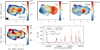 |
Fig. 11 Column density (top left panel), velocity offset (top middle panel), full width at half maximum linewidth (top right panel), and rotational temperature (bottom left panel) maps obtained by fitting CH3CN (12K−11K), K = 4−6 and |


4.3 Massestimates
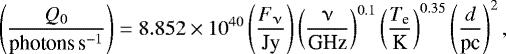
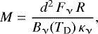
The combined bolometric luminosity of W3(H2O) and W3(OH), determined from fitting the SED from the near-IR to sub-mm, is 8.3 × 10⁴ L⊙ (Mottram et al. 2011). The contribution from OH can be estimated by first calculating the corresponding flux of ionising photons (see e.g. Appendix B.2 of Sánchez-Monge 2011, for more details) using
 (1)
(1)
where Fν is the flux density of the free–free radio continuum emission at frequency ν, Te is the electron temperature, and d is the distance. The observed integrated radio flux at 15 GHz for W3(OH) is 2.53 Jy (Kurtz et al. 1994), and assuming a typical electron temperature of 104 K, this results in a value of Q0 = 1.2 × 1048 photons s−1. Interpolating from Table 1 of Davies et al. (2011) and the relationships between spectral type and photospheric temperature from Martins et al. (2005) and Boehm-Vitense (1981) for O and B stars, respectively, this ionising photon flux approximately corresponds to an O8.5 main sequence star, with M ≈ 20M⊙ and L ≈ 4.4 × 10⁴ L⊙. This leaves a total bolometric luminosity of 3.9 × 10⁴ L⊙, which we assume to be evenly distributed between the two cores within W3(H2O), 1.95 × 10⁴ L⊙ each; using the same tables this would correspond to two 15 M⊙ stars of spectral type B0.
The above estimates are based on Davies et al. (2011) for zero age main sequence (ZAMS) stars. High-mass protostars growing by accretion resemble ZAMS stars in terms of their luminosities and temperatures when core nuclear burning dominates other sources of luminosity such as accretion and envelope burning. When this occurs depends primarily on when the protostar gains sufficient mass, but also on the accretion rate. Stellar structure calculations suggest that this occurs at 5–10 M⊙ for accretion rates of 10−5–10−4 M⊙ yr−1, respectively (Norberg & Maeder 2000; Behrend & Maeder 2001; Keto & Wood 2006). The mass estimates further assume that all the emitted energy has been produced within the (proto)stars, ignoring contributions from episodic accretion to the luminosity. Therefore, the 15 M⊙ estimates can be taken as upper limits, in agreement with calculations of Chen et al. (2006) who find a minimum binary mass of 22 M⊙ for the protostars within W3(H2O). Furthermore, assuming the gas to be in gravito-centrifugal rotation around the two individual cores, our PV plots (see Fig. 10) suggest that the range of 5− 15 M⊙ is a reasonable estimate for the protostellar masses.
As dust is typically optically thin in the 1.3 mm wavelength regime and proven to be for this region in particular (Chen et al. 2006), we use the prescription by Hildebrand (1983) to convert the flux density, Fν, of the continuum observations to a mass. In the form presented by Schuller et al. (2009),
 (2)
(2)
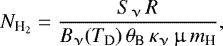
where R is the gas-to-dust mass ratio, Bν(TD) is the Planck function at a dust temperature of TD, and κν is the dust absorption coefficient. We adopt a gas-to-dust mass ratio of R = 150 (Draine 2011) and a value of κν = 0.9 cm2 g−1 for the dust absorption coefficient from Ossenkopf & Henning (1994), corresponding to thin ice mantles after 105 yr of coagulation at a density of 106 cm−3.
High-mass cores, such as the ones we are studying, typically have densities high enough to thermalise the methyl cyanide lines. To check this, using the spontaneous decay rate of CH 3CN (124−114) obtained from the LAMDA database5, 7.65× 10⁻⁴ s−1, and the collision rate of 2.05 × 10⁻¹⁰ cm3 s−1 with H2 at 140 K (Green 1986), we calculate the simplified two-level critical density of this line to be ncrit ≈ 3.7 × 106 cm−3. The effective density, once the radiation field is taken into account, is typically an order of magnitude lower (Evans 1999; Shirley 2015). Following Schuller et al. (2009), the H2 column density is calculated via
 (3)
(3)
where Sν is the peak intensity, θB is the beam solid angle, μ is the mean molecular weight assumed to be equal to 2.8, and mH is the mass of the hydrogen atom. At a temperature of 140 K and using our continuum intensity of a given position near the centre, we can estimate the H2 column density to be 4.5 × 1024 cm−2. This can be converted to a volume density of 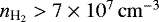 , assuming the maximum extent of the third dimension to be the plane-of-sky size of the clump (~4000 AU). Therefore, since the density of molecular hydrogen is much higher than the critical density of the lines, the LTE assumption is valid and the rotational temperature map of CH3CN obtained from our modelling can be assumed to be tracing the gas kinetic temperature.
Using Eq. (2), our continuum map with its unit converted to Jy pixel−1 and the temperature map obtained from XCLASS, assuming dust and gas temperatures are coupled, we obtain a pixel-by-pixel mass density map (see Fig. C.1). Summing over the pixels in our mass density map in the ABD observations, the total mass for W3(H2O) is calculated to be ~26.8 M⊙, with 15.4 M⊙ contributed from the core to the east, and 11.4 M⊙ from the core to the west. Similarly, using the AB observations, we obtain a total mass of ~11.4 M⊙ for W3(H2O), with a core mass of 6.7 and 4.7 M⊙ from the cores to the east and west, respectively. The effect of spatial filtering of the interferometer is clear in these mass estimates as the exclusion of the D-array data removes more than half of the mass.
Comparing our NOEMA observations to SCUBA-2 850 μm single-dish observations, about 25% of the flux is filtered out by the interferometer in our ABD observations (assuming a ν−3.5 frequency-relation; Beuther et al. 2018), implying that our core mass estimates of 15.4 and 11.4 M⊙ are lower limits, but nevertheless reasonable. Masses estimated in this manner have contributions from the cores and the disk-like structures and not from any embedded (proto)stars.
4.4 Toomre stability
For a differentially rotating disk, the shear force and gas pressure can provide added stability against gravitational collapse. This idea was originally introduced by Safronov (1960) and further quantified by Toomre (1964) for a disk of stars, and has since been used in various applications ranging from planet formation to galaxy dynamics. We investigate the stability of the rotating structures in W3(H2O), assuming that they are disks in gravito-centrifugal equilibrium, against axisymmetric instabilities using the Toomre Q parameter,
 (4)
(4)
where cs is the sound speed, and Ω is the epicyclic frequency of the disk which is equivalent to its angular velocity. The surface density of the disk, Σ, is calculated by multiplying the column density (Eq. (3)) by the mean molecular weight and mass of the hydrogen atom (μmH) to convert the number column density to a mass surface density. A thin disk becomes unstable against axisymmetric gravitational instabilities if Q < 1.
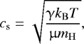
Having obtained a temperature map representative of the kinetic temperature, we are able to calculate the Toomre Q parameter pixel by pixel. In particular, the temperature is used in the calculation of Bν (TD) and the sound speed,
 (5)
(5)
where γ is the adiabatic index with avalue of 5∕3.
We assume two 10 M⊙ (proto)stellar objects to be present, one at the position of each of the two continuum peaks (see AB image in Fig. 4). The angular velocity maps are created by adding up mass within concentric circles starting at the position of each core and going outwards. In this way, we incorporate the mass of the rotating structures, calculated via Eq. (2), and the mass of the central objects. The angular velocity of a disk in gravito-centrifugal equilibrium at a radius r is
 (6)
(6)
where the mass of the central object, M*, is 10 M⊙ and Mdisk(r) is the gas mass enclosed within r. Given the radii involved, this means that in practice, most parts of the maps are dominated by Mdisk rather than M*.
In Fig. 12, we present our Toomre Q map of W3(H2O), which is created by stitching together the Toomre Q maps of the two individual cores. The stitching boundary is shown by a solid vertical line and the positions of the two central objects corresponding to our continuum peaks in the AB image (see Fig. 4) are indicated by stars. While the Toomre Q calculations were performed on the AB-array data, we have drawn the continuum contours from the A-array only observations. The boundary where Q = 1 is shown by a dashed line.
The most significant factor stabilising the disk against Toomre instability is the high gas temperatures and the fastdifferential rotation of material closest to the (proto)star; therefore, we find the highest Toomre Q values closest to the presumed locations of the (proto)stars depicted by stars in Fig. 12 as expected. We find low Toomre Q values at the periphery of W3(H2O) E and W, suggesting that both rotating structures are only marginally stable against axisymmetric instabilities. Moreover, W3(H2O) W shows low Toomre Q values at the positions of additional continuum peaks in the highest resolution A-array data (solid contours in Fig. 12), suggesting further fragmentation at these positions may be possible. As the dimensions of the observed continuum peaks are smaller than the size of our synthesised beam, the validity of this hypothesis needs to be confirmed with higher resolution observations(at 345 GHz) to be taken with NOEMA.
A Toomre stability analysis performed by Chen et al. (2016) for the high-mass protostar IRAS 20126+4104showed that the massive disk around that protostar is hot and stable to fragmentation, with Toomre Q > 2.8 at all radii. Hydrodynamic simulations of collapsing protostellar cores by Klassen et al. (2016) find massive accretion disks which evolve to become asymmetrically Toomre-unstable, creating large spiral arms with an increased rate of accretion of material onto the central object. They find that the self-gravity of these spiral arm segments is lower than the tidal forces from the star, causing the spiral arms in their simulations to remain stable against collapse. However, they find that the Toomre conditions combined with the cooling of the disk (Gammie 2001) would potentially yield the formation of a binary companion. Similarly, simulations by Kuiper et al. (2011) see such spiral arms in a massive disk, and simulations by Krumholz et al. (2009) and more recently Meyer et al. (2017, 2018) see disk fragmentation on even smaller spatial scales, on the order of hundreds of AU. Therefore, disk fragmentation scenarios in the high-mass regime are valid from a theoretical stand point.
Among the assumptions that go into this Toomre analysis is the thin-disk approximation. According to Gammie (2001), the critical value of Q for an isothermal disk of finite thickness should be 0.676 (as derived from Goldreich & Lynden-Bell 1965). Even with such a low critical value, the rotating structures around each core would still show signs of instability in their outskirts. To get an estimate on the importance of disk thickness, following Gammie (2001), the instability condition for a disk with scale height, H ≃ cs∕Ω, can be written as
 (7)
(7)
Using our temperature and angular velocity maps, we create a map of the H∕r ratio. In this way, we calculate an average value of H∕r ≈ 0.3. Assuming the mass of each (proto)star is roughly 10 M⊙, we calculate that for the candidate disks to be unstable against gravitational collapse, the mass of the candidate disk must be Mdisk ≳ 3 M⊙. Since the mass estimates for the cores obtained from the continuum maps using Eq. (2) are 15 and 11 M⊙, the masses are large enough to result in the rotating structures being Toomre-unstable. Therefore, the thickness of the candidate disks does not affect the general interpretation of our results.
The angular velocity maps used in the calculation of the Toomre Q map have been created assuming a face-on geometry for the candidate disks. If the objects are inclined, we would be overestimating the surface density of the candidate disks and the line-of-sight angular velocities. Since these two parameters have the opposite effect on the Toomre Q value (see Eq. (4)), our results are still reasonable. Furthermore, W3(H2O) E may harbour multiple (proto)stars within it (see Sect. 4.1) such that the possibility of rotational contributions from multi-body rotation would require a different prescription for the epicyclic frequency than what we have assumed.
The estimation of 10 M⊙ for the central (proto)stars have been deduced from our own and previous mass estimations (see Sect. 4.3), and by examining the emission in the PV plots with Keplerian curves that are just “grazing” the emission. The latter method has the caveat that the observed PV plot is the result of the convolution with the instrumental beam and the line width. Therefore, the real emission is less extended in space and velocity than we observe, and as a result we may be overestimating the mass of the (proto)stars. Performing our Toomre calculations, but with the assumption of 5 M⊙ (proto)stars, we obtain median Toomre Q values of 1.3 compared to a value of 1.7 in the 10 M⊙ calculations. Therefore, lower protostellar masses would lead to the decrease in the Toomre Q value, and thus larger unstable regions, making the disk fragmentation scenario even more plausible. On the other hand, as the mass estimates using the bolometric luminosities suggest the central (proto)stellar masses to be in the 15 M⊙ regime, the median Toomre Q value would be 2.0, with unstable regions still present in the outskirts. The Toomre Q maps created assuming two 5 and 15 M⊙ (proto) stars at the position of the continuum peaks can be found in Appendix D. The change of ±5 M⊙ does not strongly affect the Toomre Q maps because we add the mass of the candidate disks, estimated from the continuum emission to be 15 and 11 M⊙, in rings (see Eq. (6)) and they dominate over an addition or subtraction of 5 M⊙, especially in the outermost regions. This, together with the root dependence on mass lead to uncertainties in M* to only have a small effect on the Toomre Q results.
We are currently conducting simulated observations from 3D hydrodynamic simulations to investigate the reliability of our methods in even more depth (Ahmadi et al. in prep.). Our preliminary results on the effect of inclination and (proto)stellar mass on the calculation of Toomre Q maps using hydrodynamic simulations suggest that the Toomre Q value is not strongly dependent on these parameters. A forthcoming paper is dedicated to this topic.
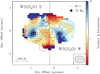 |
Fig. 12 Toomre Q map obtained by assuming two disk-like structures in gravito-centrifugal rotation about the positions of peak continuum emission as depicted by the two stars, each with a mass of 10 M⊙. The Toomre Q calculations and the positions of (proto)stars are based on the AB-array data (see Fig. 4) with regions outside the 6σ mm continuum emission masked out. Solid contours correspond to our continuum data in the most extended configuration (A-array), starting at 6σ and increasing in steps of 3σ (1σ = 2.5 mJy beam−1). The solid vertical line corresponds to the stitching boundary. The dashed lines correspond to Q = 1. |
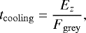
4.5 Cooling
For a marginally stable disk (Q ~ 1), the locally unstable regions compress as they start to collapse, providing compressional heating in these regions. This increase in the local thermal pressure can counteract the local collapse and put the disk back into a state of equilibrium such that the region will not fragment unless heat can be dissipated on a short timescale. Through numerical simulations, Gammie (2001) and Johnson & Gammie (2003) have introduced a cooling parameter, β, to study the effect of cooling for marginally stable thin disks in gravito-centrifugal equilibrium. In their prescription
 (8)
(8)
where the cooling time, tcooling, is assumed to be constant and a function of the surface density and internal energy of the disk. If the local collapse needs more than a few orbits, due to a long cooling timescale, a locally collapsing region within the disk can be ripped apart by shear. Therefore, there is a critical β value below which a locally collapsing region would be rapidly cooling, and if it is sufficiently self-gravitating, it would be prone to fragmentation. Conversely, values above this critical β value would put a marginally stable disk into a self-regulating scenario such that heating acts as a stabilising force and directly counteracts the cooling rate.
The Gammie cooling criterion is relevant only if the disk is marginally stable, with regions that are locally unstable against axisymmetric gravitational instabilities. A Toomre-stable disk will not fragment regardless of how quickly it may be cooling.
This critical value is determined through numerical simulations and varies depending on the heating and cooling recipes and convergence issues. For an overview of these issues, see Kratter & Lodato (2016) and Baehr et al. (2017). Regardless of the specific numerical simulation issues, it is generally assumed that the critical β value rangesbetween 1 and 5.
Following the prescription of Klassen et al. (2016),
 (9)
(9)
where Ez is the column internal energy integrated in the z-direction (along the axis of rotation) and Fgrey is the radiative flux away from the disk adopting a grey-body approximation. The internal energy of an ideal gas is calculated via
 (10)
(10)
where ρ is the volume density and cv is the specific heat capacity defined as
 (11)
(11)
with NA as Avogadro’s number and Mu the molar mass. By replacing the volume density with the surface density, the column internal energy is then
 (12)
(12)
Knowing the cooling time, which is of the order of months, and the rotation rate at each pixel, we construct a local β map. Figure 13 shows the β map for the two disks presumed in gravito-centrifugal equilibrium about the positions of peak continuum emission as depicted by stars. The median β value is 1.8 × 10⁻⁴, and the maximum value found in the outskirts is on the order of 10−2, which is much lower than the critical value of 1–5. This finding is consistent with that of Klassen et al. (2016) and Meyer et al. (2018) who also find β ≪ 1 in their simulation of collapsing protostellar cores with a mass of 100 M⊙ at later times. The rotating bodies within W3(H2O) are therefore able to cool rapidly and any local collapse induced by the gravitational instabilities in the disks will lead to fragmentation. Rapid cooling in this context means that the cooling timescale is comparable to the local dynamical timescale.
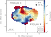 |
Fig. 13 Map of β cooling parameter obtained by assuming two disk-like structures in gravito-centrifugal rotation about the positions of peak continuum emission as depicted by stars. The solid contours correspond to our continuum data in the most extended configuration, starting at 6σ and increasing in steps of 3σ (1σ = 2.5 mJy beam−1). The solid vertical line corresponds to the stitching boundary. The dashed line corresponds to Toomre Q = 1. Regions outside of the 6σ mm continuum emission contour in the AB configuration are masked out. |
5 Conclusions and summary
Our IRAM large programme, CORE, aims to study fragmentation and the kinematics of a sample of 20 high-mass star-formingregions. We have performed a case-study for one of the sources in our sample, the prototypical hot core W3(H2O). In this paper we present details of the spectral line setup for our NOEMA observations in the 1.37 mm band which covers transitions of important tracers of dense gas and disks (e.g. CH3CN, HCOOCH3, CH3OH), inner envelopes (e.g. H2CO), and outflows (e.g. 13CO, SO). We cover the range of 217 078.6−220 859.5 MHz with a spectral resolution of 2.7 km s−1, and eight narrower bands centred on specific transitions to provide higher spectral resolution of 0.5 km s−1.
With the aim of studying the fragmentation and kinematic properties of W3(H2O), the following is a summary of our findings:
At an angular resolution of ~0.′′35 (~700 AU at 2 kpc), W3(H2O) fragments into two cores, which we refer to as W3(H2O) E and W3(H2O) W, separated by ~2300 AU, as seen in both line and thermal dust continuum emission.
Based onthe integrated dust continuum emission, W3(H2O) has a total mass of ~26.8 M⊙, with 15.4 M⊙ contributed from W3(H2O) E, and 11.4 M⊙ from W3(H2O) W.
On large scales, there is a clear velocity gradient in the east–west direction across W3(H2O), spanning ~6000 AU, attributed to a combination of circumbinary and circumstellar motions. On smaller scales, velocity gradients of a few km s−1 are observed across each of the cores, perpendicular to the directions of two bipolar molecular outflows, one emanating from each core, as traced by 12CO and 13CO. The direction of motion of the gas around the individual cores deviates little from the overall larger scale rotation of W3(H2O), suggesting that these motions seen around the cores, which we interpret as rotation, may be inherited from the large-scale rotation.
The kinematics of the rotating structure about W3(H2O) W shows differential rotation of material about a (proto)star as deduced from the redshifted part of its PV plot, suggesting that the rotating structure may be a disk-like object. The radio source with a rising spectrum at this position can be attributed to a circumstellar jet or wind ionised by the embedded (proto)star at this position.
The PV plots of the rotating structure about W3(H2O) E is inconclusive on whether the observed rotation is due to a disk-like rotating object, an unresolved binary (or multiple) system, or a combination of the two.
We fit the emission of CH3CN (12K−11K), K = 4−6 and
 with XCLASS and produce temperature, column density, peak velocity, and velocity dispersion maps. On average, the entire structure is hot (~165 K) with no particular temperature structure. The column density map of CH3CN is double peaked, similar to the continuum and line emission maps, with a median column density of ~1.4 × 1015 cm-2. Close to the centre of the cores the H2 column density is estimated to be ~ 5 × 1024 cm-2.
-
We investigate the axisymmetric stability of the two rotating structures using the Toomre criterion. Our Toomre Q map shows low values in the outskirts of both rotating structures, suggesting that they are unstable to fragmentation. Some regions with low Toomre Q values in the vicinity of W3(H2O) W coincidewith unresolved thermal dust continuum peaks (in our highest resolution observations), hinting at the possibility of further fragmentation in this core.
-
The Toomre-unstable regions within W3(H2O) E and W3(H2O) W are able to cool rapidly, and any local collapse induced by the gravitational instabilities will lead to further fragmentation.
In this work, we showcase our in-depth analysis for the kinematics and stability of the rotating structures within W3(H2O). We showed that high-mass cores can be prone to fragmentation induced by disk instabilities at ~1000 AU scales, and core fragmentation at larger scales. Therefore, different modes of fragmentation contribute to the final stellar mass distribution of a given region. One question still remains: How universal are these findings? To this end, we aim to benchmark our methods using hydrodynamic simulations and extend our analysis to the full CORE sample in future papers.
Acknowledgements
The authors would like to thank the anonymous referee whose comments helped the clarity of this paper. We also thank Thomas Möller for his technical support with the XCLASS analysis, and Kaitlin Kratter for fruitful discussions regarding the Toomre Q stability analysis. A.A., H.B., J.C.M., and F.B. acknowledge support from the European Research Council under the European Community’s Horizon 2020 framework programme (2014–2020) via the ERC Consolidator Grant “From Cloud to Star Formation (CSF)” (project number 648505). R.K. acknowledges financial support via the Emmy Noether Research Group on Accretion Flows and Feedback in Realistic Models of Massive Star Formation funded by the German Research Foundation (DFG) under grant no. KU 2849/3-1. T.Cs. acknowledges support from the Deutsche Forschungsgemeinschaft, DFG via the SPP (priority programme)1573 “Physics of the ISM”. A.P. acknowledges financial support from UNAM and CONACyT, México.
Appendix A Moment maps
In this section, we present zeroth (Fig. A.1), first (Fig. A.2), and second (Fig. A.3) moment maps of various detected lines in the narrow-band receiver for W3(H2O) (top panels) and W3(OH) (bottom panels) in the combined A-, B-, and D-array observations. All moment maps have been created inside regions where the S/N is greater than5σ.
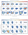 |
Fig. A.1 Integrated intensity (zeroth moment) maps of most important lines covered in the narrow-band receiver for the observations in the ABD configuration for W3(H2O) (top panel) and W3(OH) (bottom panel). The solid contours correspond to the dust continuum and start at and increase by 6σ (1σ = 3.2 mJy beam−1). The sizeof the synthesised beam is shown in the bottom left of each panel. The map of CH3CN (125−115) may not be accurate because it is blended with other lines. |
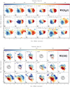 |
Fig. A.2 Intensity-weighted peak velocity (first moment) maps of most important lines covered in the narrow-band receiver for the observations in the ABD configuration for W3(H2O) (top panel) and W3(OH) (bottom panel). The solid contours correspond to the dust continuum and start at and increase by 6σ (1σ = 3.2 mJy beam−1). The sizeof the synthesised beam is shown in the bottom left of each panel. The map of CH3CN (125−115) may not be accurate because it is blended with other lines. |
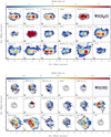 |
Fig. A.3 Root mean square velocity dispersion (second moment) maps of most important lines covered in the narrow-band receiver for the observations in the ABD configuration for W3(H2O) (top panel) and W3(OH) (bottom panel). The solid contours correspond to the dust continuum and start at and increase by 6σ (1σ = 3.2 mJy beam−1). The sizeof the synthesised beam is shown in the bottom left of each panel. The map of CH3CN (125−115) may not be accurate because it is blended with other lines. |
Appendix B Details of XCLASS fitting
XCLASS explores the parameter space (source size, column density, temperature, linewidth, and peak velocity) using as many algorithms as the user demands, and stops when the maximum number of iterations has been reached. In our analysis, we employed a combination of the Genetic and Levenberg–Marquardt algorithms6, and an isothermal model such that one temperature is used to reproduce the observed population of lines for a given species in a given spectrum. We assumed that the size of the source was larger than the beam and therefore did not fit the beam filling factor parameter. Our initial fits to the spectra of CH 3CN included the full K = 0−6 ladder, along with its  isotopologue, prescribing the 12C/13C ratio to be 76, which is consistent with the findings of Henkel et al. (1982) and the calculations of Qin et al. (2015) for W3(H2O). The top panel of Fig. B.1 shows an example of the best-fit spectrum for one pixel in the AB observations, which yielded a high rotational temperature of 835 K. The lower intensities of the low-K lines of CH 3CN compared to the transitions higher on the K-ladder indicates that the low-K transitions are optically thick. Furthermore, the fits to the optically thinner high-K lines are not satisfactory. Repeating the same procedure, but only fitting the CH 3CN (12K−11K), K = 4−6 lines along with the
  isotopologues results in a better fit to these lines for a lower rotational temperature of 207 K (see bottom panel of Fig. B.1). These findings are in agreement with line fitting analysis of Feng et al. (2015) in Orion KL in which they find that fitting all CH 3CN lines, assuming they are optically thin and in LTE, yields higher temperatures than when fitting them with an optical depth correction (see their Fig. 8). The exclusion of the optically thick and low-energy lower-K lines along with the inclusion of the 13C isotopologues, although barely detected, allows the software to avoid prioritising the fitting of these optically thick lines and therefore derives the temperature more accurately. This finding is also related to the existence of temperature and density gradients which our one-component model cannot properly reproduce. As lower-K lines are more easily excited than the higher-K lines, they can probe the temperature in the envelope and in the disk surface, while the higher-K lines are better at tracing the disk and may not be as excited in the envelope. In fact, the reason why the brightness temperature of the low-K lines is lower than the high-K lines may be due to self-absorption of the photons from the warmer inner region by molecules in the cooler envelope material between the disk and the observer. Another explanation can be that the optically thick low-K transitions are more extended and therefore may be partially resolved out.
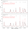 |
Fig. B.1 Top panel: spectrum of a given pixel (in black) along with the XCLASS fit for CH3CN (12K−11K), K = 0−6 and |


Appendix C Mass density map
In this section we present the mass density map for W3(H2O) in Fig. C.1, which was constructed using Eq. (2) with the continuum map converted to Jy pixel−1 units, and the temperature map obtained from modelling CH3CN (12K−11K), K = 4−6 lines with XCLASS. This map is used in the calculation of the angular velocity in the construction of the Toomre Q map.
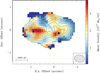 |
Fig. C.1 Mass density map obtained using the temperature and continuum maps in Eq. (2). The solid contours correspond to our continuum observations in the AB configuration, starting at 6σ and increasing in steps of 3σ (1σ = 2.5 mJy beam−1). Each of the peak continuum positions, as depicted by stars, is expected to host at least one 10 M⊙ (proto)star or more lower mass sources. |
Appendix D Toomre Q maps
In Fig. D.1, we present Toomre Q maps created assuming either two 5 M⊙ (proto)stars at the positions of the two continuum peaks (top panel), or two 15 M⊙ (proto)stars (bottom panel).
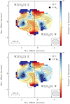 |
Fig. D.1 Toomre Q map obtained by assuming two disks in gravito-centrifugal rotation about two 5 M⊙ (proto)stars (top panel) and two 15 M⊙ (proto)stars (bottom panel) at the positions of peak continuum emission as depicted by the two stars. The solid contours correspond to our continuum data in the most extended configuration, starting at 6σ and increasing in steps of 3σ (1σ = 2.5 mJy beam−1). The solid vertical line corresponds to the stitching boundary. The dashed line corresponds to Q = 1. Regions outside of the 6σ mm continuum emission contour in the AB configuration are masked out. |
References
- Baehr, H., Klahr, H., & Kratter, K. M. 2017, ApJ, 848, 40 [NASA ADS] [CrossRef] [Google Scholar]
- Behrend, R., & Maeder, A. 2001, A&A, 373, 190 [NASA ADS] [CrossRef] [EDP Sciences] [Google Scholar]
- Beltrán, M. T., & de Wit W. J. 2016, A&ARv, 24, 6 [NASA ADS] [CrossRef] [Google Scholar]
- Beltrán, M. T., Cesaroni, R., Neri, R., et al. 2005, A&A, 435, 901 [NASA ADS] [CrossRef] [EDP Sciences] [Google Scholar]
- Beltrán, M. T., Sánchez-Monge, Á., Cesaroni, R., et al. 2014, A&A, 571, A52 [NASA ADS] [CrossRef] [EDP Sciences] [Google Scholar]
- Beuther, H., Schilke, P., Gueth, F., et al. 2002, A&A, 387, 931 [NASA ADS] [CrossRef] [EDP Sciences] [Google Scholar]
- Beuther, H., Zhang, Q., Sridharan, T. K., & Chen, Y. 2005, ApJ, 628, 800 [NASA ADS] [CrossRef] [Google Scholar]
- Beuther, H., Zhang, Q., Hunter, T. R., Sridharan, T. K., & Bergin, E. A. 2007, A&A, 473, 493 [NASA ADS] [CrossRef] [EDP Sciences] [Google Scholar]
- Beuther, H., Mottram, J. C., Ahmadi, A., et al. 2018, A&A, 617, A100 [NASA ADS] [CrossRef] [EDP Sciences] [Google Scholar]
- Boehm-Vitense, E. 1981, ARA&A, 19, 295 [NASA ADS] [CrossRef] [Google Scholar]
- Bontemps, S., Motte, F., Csengeri, T., & Schneider, N. 2010, A&A, 524, A18 [NASA ADS] [CrossRef] [EDP Sciences] [Google Scholar]
- Carrasco-González, C., Galván-Madrid, R., Anglada, G., et al. 2012, ApJ, 752, L29 [NASA ADS] [CrossRef] [Google Scholar]
- Cesaroni, R., Galli, D., Lodato, G., Walmsley, C. M., & Zhang, Q. 2007, in Protostars and Planets V, eds. B. Reipurth, D. Jewitt, & K. Keil (Tucson, AZ: Arizona University Press), 197 [Google Scholar]
- Cesaroni, R., Sánchez-Monge, Á., Beltrán, M. T., et al. 2017, A&A, 602, A59 [NASA ADS] [CrossRef] [EDP Sciences] [Google Scholar]
- Chen, H.-R., Welch, W. J., Wilner, D. J., & Sutton, E. C. 2006, ApJ, 639, 975 [NASA ADS] [CrossRef] [Google Scholar]
- Chen, H.-R. V., Keto, E., Zhang, Q., et al. 2016, ApJ, 823, 125 [NASA ADS] [CrossRef] [Google Scholar]
- Clark, B. G. 1980, A&A, 89, 377 [NASA ADS] [Google Scholar]
- Davies, B., Hoare, M. G., Lumsden, S. L., et al. 2011, MNRAS, 416, 972 [NASA ADS] [CrossRef] [Google Scholar]
- Draine, B. T. 2011, Physics of the Interstellar and Intergalactic Medium (Princeton: Princeton University Press) [Google Scholar]
- Dreher, J. W., & Welch, W. J. 1981, ApJ, 245, 857 [NASA ADS] [CrossRef] [Google Scholar]
- Evans, II, N. J. 1999, ARA&A, 37, 311 [NASA ADS] [CrossRef] [Google Scholar]
- Fallscheer, C., Beuther, H., Zhang, Q., Keto, E., & Sridharan, T. K. 2009, A&A, 504, 127 [NASA ADS] [CrossRef] [EDP Sciences] [Google Scholar]
- Feng, S., Beuther, H., Henning, T., et al. 2015, A&A, 581, A71 [NASA ADS] [CrossRef] [EDP Sciences] [Google Scholar]
- Frank, A., Ray, T. P., Cabrit, S., et al. 2014, in Protostars and Planets VI, eds. H. Beuther, R. Klessen, C. Dullemond, & T. Henning (Tucson, AZ: University of Arizona Press), 451 [Google Scholar]
- Gammie, C. F. 2001, ApJ, 553, 174 [NASA ADS] [CrossRef] [Google Scholar]
- Goldreich, P., & Lynden-Bell, D. 1965, MNRAS, 130, 125 [NASA ADS] [CrossRef] [Google Scholar]
- Green, S. 1986, ApJ, 309, 331 [NASA ADS] [CrossRef] [Google Scholar]
- Hachisuka, K., Brunthaler, A., Menten, K. M., et al. 2006, ApJ, 645, 337 [NASA ADS] [CrossRef] [Google Scholar]
- Henkel, C., Wilson, T. L., & Bieging, J. 1982, A&A, 109, 344 [NASA ADS] [Google Scholar]
- Hildebrand, R. H. 1983, QJRAS, 24, 267 [NASA ADS] [Google Scholar]
- Ilee, J. D., Cyganowski, C. J., Nazari, P., et al. 2016, MNRAS, 462, 4386 [NASA ADS] [CrossRef] [Google Scholar]
- Johnson, B. M., & Gammie, C. F. 2003, ApJ, 597, 131 [NASA ADS] [CrossRef] [Google Scholar]
- Johnston, K. G., Robitaille, T. P., Beuther, H., et al. 2015, ApJ, 813, L19 [NASA ADS] [CrossRef] [Google Scholar]
- Kahn, F. D. 1974, A&A, 37, 149 [NASA ADS] [Google Scholar]
- Keto, E., & Wood, K. 2006, ApJ, 637, 850 [NASA ADS] [CrossRef] [Google Scholar]
- Keto, E. R., Welch, W. J., Reid, M. J., & Ho, P. T. P. 1995, ApJ, 444, 765 [NASA ADS] [CrossRef] [Google Scholar]
- Klassen, M., Pudritz, R. E., Kuiper, R., Peters, T., & Banerjee, R. 2016, ApJ, 823, 28 [NASA ADS] [CrossRef] [Google Scholar]
- Kratter, K., & Lodato, G. 2016, ARA&A, 54, 271 [NASA ADS] [CrossRef] [Google Scholar]
- Krumholz, M. R., Klein, R. I., McKee, C. F., Offner, S. S. R., & Cunningham, A. J. 2009, Science, 323, 754 [NASA ADS] [CrossRef] [PubMed] [Google Scholar]
- Kuiper, R., & Yorke, H. W. 2013, ApJ, 772, 61 [NASA ADS] [CrossRef] [Google Scholar]
- Kuiper, R., Klahr, H., Beuther, H., & Henning, T. 2010, ApJ, 722, 1556 [CrossRef] [Google Scholar]
- Kuiper, R., Klahr, H., Beuther, H., & Henning, T. 2011, ApJ, 732, 20 [NASA ADS] [CrossRef] [Google Scholar]
- Kurtz, S., Churchwell, E., & Wood, D. O. S. 1994, ApJS, 91, 659 [NASA ADS] [CrossRef] [Google Scholar]
- Leurini, S., Codella, C., Zapata, L., et al. 2011, A&A, 530, A12 [NASA ADS] [CrossRef] [EDP Sciences] [Google Scholar]
- Loren, R. B., & Mundy, L. G. 1984, ApJ, 286, 232 [NASA ADS] [CrossRef] [Google Scholar]
- Martins, F., Schaerer, D., & Hillier, D. J. 2005, A&A, 436, 1049 [NASA ADS] [CrossRef] [EDP Sciences] [Google Scholar]
- Matsumoto, T., & Hanawa, T. 2003, ApJ, 595, 913 [NASA ADS] [CrossRef] [Google Scholar]
- Maud, L. T., Moore, T. J. T., Lumsden, S. L., et al. 2015, MNRAS, 453, 645 [NASA ADS] [CrossRef] [Google Scholar]
- Meyer, D. M.-A., Vorobyov, E. I., Kuiper, R., & Kley, W. 2017, MNRAS, 464, L90 [NASA ADS] [CrossRef] [Google Scholar]
- Meyer, D. M.-A., Kuiper, R., Kley, W., Johnston, K. G., & Vorobyov, E. 2018, MNRAS, 473, 3615 [NASA ADS] [CrossRef] [Google Scholar]
- Möller, T., Endres, C., & Schilke, P. 2017, A&A, 598, A7 [NASA ADS] [CrossRef] [EDP Sciences] [Google Scholar]
- Motte, F., Bontemps, S., & Louvet, F. 2018, ARA&A, 56, 41 [NASA ADS] [CrossRef] [Google Scholar]
- Mottram, J. C., Hoare, M. G., Urquhart, J. S., et al. 2011, A&A, 525, A149 [NASA ADS] [CrossRef] [EDP Sciences] [Google Scholar]
- Mottram, J. C., et al. 2018, A&A, submitted [Google Scholar]
- Müller, H. S. P., Thorwirth, S., Roth, D. A., & Winnewisser, G. 2001, A&A, 370, L49 [NASA ADS] [CrossRef] [EDP Sciences] [Google Scholar]
- Müller, H. S. P., Schlöder, F., Stutzki, J., & Winnewisser, G. 2005, J. Mol. Struct., 742, 215 [NASA ADS] [CrossRef] [Google Scholar]
- Norberg, P., & Maeder, A. 2000, A&A, 359, 1025 [Google Scholar]
- Ohashi, N., Hayashi, M., Ho, P. T. P., & Momose, M. 1997, ApJ, 475, 211 [Google Scholar]
- Ossenkopf, V., & Henning, T. 1994, A&A, 291, 943 [NASA ADS] [Google Scholar]
- Palau, A., Fuente, A., Girart, J. M., et al. 2013, ApJ, 762, 120 [NASA ADS] [CrossRef] [Google Scholar]
- Palau, A., Ballesteros-Paredes, J., Vázquez-Semadeni, E., et al. 2015, MNRAS, 453, 3785 [NASA ADS] [CrossRef] [Google Scholar]
- Peters, T., Banerjee, R., Klessen, R. S., et al. 2010, ApJ, 711, 1017 [NASA ADS] [CrossRef] [Google Scholar]
- Pickett, H. M., Poynter, R. L., Cohen, E. A., et al. 1998, J. Quant. Spectr. Rad. Transf., 60, 883 [NASA ADS] [CrossRef] [Google Scholar]
- Pudritz, R. E., Ouyed, R., Fendt, C., & Brandenburg, A. 2007, in Protostars and Planets V, eds. B. Reipurth, D. Jewitt, & K. Keil (Tucson, AZ: University of Arizona Press), 277 [Google Scholar]
- Qin, S.-L., Schilke, P., Wu, J., et al. 2015, ApJ, 803, 39 [NASA ADS] [CrossRef] [Google Scholar]
- Reid, M. J., Argon, A. L., Masson, C. R., Menten, K. M., & Moran, J. M. 1995, ApJ, 443, 238 [NASA ADS] [CrossRef] [Google Scholar]
- Safronov, V. S. 1960, Ann. Astrophys., 23, 979 [Google Scholar]
- Sánchez-Monge, Á. 2011, PhD Thesis, Universitat de Barcelona, Spain [Google Scholar]
- Sánchez-Monge, Á., Cesaroni, R., Beltrán, M. T., et al. 2013, A&A, 552, L10 [NASA ADS] [CrossRef] [EDP Sciences] [Google Scholar]
- Schuller, F., Menten, K. M., Contreras, Y., et al. 2009, A&A, 504, 415 [NASA ADS] [CrossRef] [EDP Sciences] [Google Scholar]
- Shchekinov, Y. A., & Sobolev, A. M. 2004, A&A, 418, 1045 [NASA ADS] [CrossRef] [EDP Sciences] [Google Scholar]
- Shirley, Y. L. 2015, PASP, 127, 299 [NASA ADS] [CrossRef] [Google Scholar]
- Steer, D. G., Dewdney, P. E., & Ito, M. R. 1984, A&A, 137, 159 [NASA ADS] [Google Scholar]
- Tobin, J. J., Hartmann, L., Bergin, E., et al. 2012, ApJ, 748, 16 [Google Scholar]
- Toomre, A. 1964, ApJ, 139, 1217 [NASA ADS] [CrossRef] [Google Scholar]
- Turner, J. L., & Welch, W. J. 1984, ApJ, 287, L81 [NASA ADS] [CrossRef] [Google Scholar]
- Williams, J. P., Blitz, L., & McKee, C. F. 2000, in Protostars and Planets IV, eds. V. Mannings, A. Boss, & S. Russell (Tucson, AZ: Arizona University Press), 97 [Google Scholar]
- Wilner, D. J., Reid, M. J., & Menten, K. M. 1999, ApJ, 513, 775 [NASA ADS] [CrossRef] [Google Scholar]
- Wolfire, M. G., & Cassinelli, J. P. 1987, ApJ, 319, 850 [NASA ADS] [CrossRef] [Google Scholar]
- Wyrowski, F., Schilke, P., Walmsley, C. M., & Menten, K. M. 1999, ApJ, 514, L43 [NASA ADS] [CrossRef] [Google Scholar]
- Xu, Y., Reid, M. J., Zheng, X. W., & Menten, K. M. 2006, Science, 311, 54 [NASA ADS] [CrossRef] [PubMed] [Google Scholar]
- Yorke, H. W.,& Sonnhalter, C. 2002, ApJ, 569, 846 [NASA ADS] [CrossRef] [Google Scholar]
- Zapata, L. A., Rodríguez-Garza, C., Rodríguez, L. F., Girart, J. M., & Chen, H.-R. 2011, ApJ, 740, L19 [NASA ADS] [CrossRef] [Google Scholar]
- Zhang, Q., Ho, P. T. P., & Ohashi, N. 1998, ApJ, 494, 636 [NASA ADS] [CrossRef] [Google Scholar]
Here a core is defined as a gravitationally bound region that forms single or multiple stars, following Williams et al. (2000).
This corresponds to the CASA robust weighting with a robustness parameter of –2.
See the XCLASS manual for algorithm descriptions.
All Tables
All Figures
|
Fig. 1 Full WideX spectrum of W3(H2O) averaged over a 4′′ × 4′′ region encompassing two cores, W3(H2O) E and W3(H2O) W, showing the chemical richness of the source. The coverage of the narrow-band correlator units are shown as horizontal green lines and labelled accordingly. The units of the spectrum have been converted from Jy beam−1 to K by multiplying the flux by 188 K Jy−1 under the Rayleigh–Jeans approximation. |
| In the text | |
|
Fig. 2 Spectra of the frequency range covered by the narrow-band correlator for the pixel at the phase centre toward W3(H2O). The name of the correlator unit is listed in the bottom left corner of each panel; some of the detected lines are marked. |
| In the text | |
|
Fig. 3 NOEMA 1.37 mm (219 GHz) continuum image toward W3(H2O) and W3(OH) in the ABD configuration. The solid contours start at 6σ and increase in steps of 6σ (1σ = 3.2 mJy beam−1). The dotted contours show the same negative levels. A scale bar and the synthesised beam (0.′′ 43×0.′′32, PA = 86°) are shown at the bottom. |
| In the text | |
|
Fig. 4 1.37 mm continuum image toward W3(H2O) observed with the A (left panel), AB (middle panel), and ABD (right panel) configurations of NOEMA. The solid contours start at 6σ and increase in steps of 3σ (see Table 4). Synthesised beams are shown in the bottom left corners of each panel, along witha scale bar in the bottom right of the right-hand panel. The black stars in the middle panel correspondto the positions of the continuum peaks, marking the locations of the two individual cores, W3(H2O) W and W3(H2O) E, with the dashed line as the approximate separation boundary. The white stars in the right panel correspond to the positions of the continuum peaks A, B, and C from Wyrowski et al. (1999). The offset zero position is the phase centre of the observations: α(J2000) = 02h 27m03. s87, δ(J2000) = 61°52′24.′′5. |
| In the text | |
|
Fig. 5 Top row: integrated intensity (zeroth moment) map of CH3CN (123−113) for W3(H2O) (left panel) and W3(OH) (right panel) in the ABD configuration. Bottom row: intensity-weighted peak velocity (first moment) map of CH3CN (123−113) for W3(H2O) (left panel) and W3(OH) (right panel) in the ABD configuration. The dashed line corresponds to the cut made for the PV plot of W3(H2O) presented in Fig. 8. The solid contours correspond to the 1.37 mm continuum, starting at 6σ and increasing in steps of 6σ (1σ = 3.2 mJy beam−1). The dotted contours correspond to the same negative levels. A scale bar and the synthesised beam (0.′′ 43×0.′′32, PA = 86°) are shown in the top right panel. |
| In the text | |
|
Fig. 6 Top left panel: intensity map of CO (2–1) emission from IRAM 30 m integrated over the velocity range from − 40 to − 20 km s−1 for the redshifted and from − 80 to − 55 km s−1 for the blueshifted gas. Contours start at 5σ and increase in steps of 5σ (1σ = 1.9 K km s−1). Top right panel: intensity map of 13CO (2–1) emission from IRAM 30 m integrated over the velocity range from − 40 to − 20 km s−1 for the redshifted and from − 80 to − 55 km s−1 for the blueshifted gas. Contours start at 3σ and increase in steps of 2σ (1σ = 0.42 K km s−1). Bottom left panel: intensity map of CO (2–1) emission obtained by Zapata et al. (2011) with the SMA integrated over the velocity range from − 45 to − 25 for the redshifted and from − 75 to − 55 for the blueshifted gas. Contours start at 5σ and increase in steps of 5σ (1σ = 1.1 mJy beam−1 km s−1). The blue and red arrows highlight the positions and directions of the CO outflows emanating from each source. Bottom right panel: intensity map of 13CO (2–1) emission from IRAM 30 m merged with NOEMA observations integrated over the velocity range from − 41 to − 30 for the redshifted and from − 70 to − 53 for the blueshifted gas. Contours start at 3σ and increase in steps of 3σ (1σ = 0.03 mJy beam−1 km s−1 for redshifted and 0.17 mJy beam−1 km s−1 for blueshifted sides). The zoom panel in the top left corner highlights the launching positions of each outflow, with the red and blue arrows showing the directions of the two bipolar outflows from Zapata et al. (2011). The rms noise used in drawing the contours of the integrated intensity maps have been determined by first creating the maps without any constraints on the minimum emission level (threshold of 0) and calculating the noise in an emission-free part of the resulting map. |
| In the text | |
|
Fig. 7 NOEMA 1.37 mm (219 GHz) continuum image toward W3(H2O) in grey with levels starting at 6σ and increasing in steps of 6σ. The black contours correspond to the cm emission from Wilner et al. (1999). The positions of H2O masers obtained from Hachisuka et al. (2006) are plotted as yellow triangles. The blue and red arrows show the directions of bipolar molecular outflows from Zapata et al. (2011; see Fig. 6). The synthesised beam size of the cm emission (0.′′ 21×0.′′19, PA = 68°) is shown in black in the bottom left corner. The synthesised beam size of our mm continuum image is shown in grey in the bottom left corner. |
| In the text | |
|
Fig. 8 Position–velocity plots of W3(H2O) for a cut in the direction of rotation as depicted by a dashed line in the bottom left panel of Fig. 5 for various species and transitions in the ABD configuration. The vertical dashed lines correspond to the centre of the cut. The vertical dotted lines correspond to the positions of continuum peaks corresponding to W3(H2O) E and W3(H2O) W. The horizontal dashed lines correspond to the LSR velocity of W3(H2O). The black contours start at 4σ and increase in steps of 6σ. The white solid, dashed, and dotted lines in the top left panel correspond to the region within which emission is expected if the gas is in a disk in Keplerian rotation about a 10, 25, 50 M⊙ star, respectively.The white curves are not fits to the rotation curve, but are drawn to guide the eye. A scale bar and a cross that corresponds to the spatial and spectral resolutions are shown in the bottom right panel. |
| In the text | |
|
Fig. 9 Intensity-weighted peak velocity (first moment) map of CH3CN (123−113) using only the A-array observations and masked out to show contributions from W3(H2O) W (top panel) and W3(H2O) E (bottom panel). The solid contours correspond to the 1.37 mm continuum in the A-array only observations and start at 6σ and increase in steps of 3σ (1σ = 2.5 mJy beam−1). The dashedlines correspond to the cuts made for the PV plots (Fig. 10). The blue and red arrows show the directions of bipolar molecular outflows (Fig. 6). A scale bar and the synthesised beam (0.′′ 39×0.′′28, PA = 88°) are shown in the bottom. The velocity ranges are different for the two cores. |
| In the text | |
|
Fig. 10 Position–velocity plots along a cut in the direction of rotation as depicted by dashed lines in Fig. 9 for a fragment to the east (left panel) and to the west (right panel). The black contours start at 4σ and increase in steps of 6σ. The white solid, dashed, and dotted lines correspond to the region within which emission is expected if the gas is in a disk in Keplerian rotation about a 5, 10, and 15 M⊙ star, respectively. The crosses in the bottom right corners correspond to the spatial and spectral resolutions. Regions to the left of the dotted vertical line in the right figure contain contributions from W3(H2O) E. |
| In the text | |
|
Fig. 11 Column density (top left panel), velocity offset (top middle panel), full width at half maximum linewidth (top right panel), and rotational temperature (bottom left panel) maps obtained by fitting CH3CN (12K−11K), K = 4−6 and |
| In the text | |
|
Fig. 12 Toomre Q map obtained by assuming two disk-like structures in gravito-centrifugal rotation about the positions of peak continuum emission as depicted by the two stars, each with a mass of 10 M⊙. The Toomre Q calculations and the positions of (proto)stars are based on the AB-array data (see Fig. 4) with regions outside the 6σ mm continuum emission masked out. Solid contours correspond to our continuum data in the most extended configuration (A-array), starting at 6σ and increasing in steps of 3σ (1σ = 2.5 mJy beam−1). The solid vertical line corresponds to the stitching boundary. The dashed lines correspond to Q = 1. |
| In the text | |
|
Fig. 13 Map of β cooling parameter obtained by assuming two disk-like structures in gravito-centrifugal rotation about the positions of peak continuum emission as depicted by stars. The solid contours correspond to our continuum data in the most extended configuration, starting at 6σ and increasing in steps of 3σ (1σ = 2.5 mJy beam−1). The solid vertical line corresponds to the stitching boundary. The dashed line corresponds to Toomre Q = 1. Regions outside of the 6σ mm continuum emission contour in the AB configuration are masked out. |
| In the text | |
|
Fig. A.1 Integrated intensity (zeroth moment) maps of most important lines covered in the narrow-band receiver for the observations in the ABD configuration for W3(H2O) (top panel) and W3(OH) (bottom panel). The solid contours correspond to the dust continuum and start at and increase by 6σ (1σ = 3.2 mJy beam−1). The sizeof the synthesised beam is shown in the bottom left of each panel. The map of CH3CN (125−115) may not be accurate because it is blended with other lines. |
| In the text | |
|
Fig. A.2 Intensity-weighted peak velocity (first moment) maps of most important lines covered in the narrow-band receiver for the observations in the ABD configuration for W3(H2O) (top panel) and W3(OH) (bottom panel). The solid contours correspond to the dust continuum and start at and increase by 6σ (1σ = 3.2 mJy beam−1). The sizeof the synthesised beam is shown in the bottom left of each panel. The map of CH3CN (125−115) may not be accurate because it is blended with other lines. |
| In the text | |
|
Fig. A.3 Root mean square velocity dispersion (second moment) maps of most important lines covered in the narrow-band receiver for the observations in the ABD configuration for W3(H2O) (top panel) and W3(OH) (bottom panel). The solid contours correspond to the dust continuum and start at and increase by 6σ (1σ = 3.2 mJy beam−1). The sizeof the synthesised beam is shown in the bottom left of each panel. The map of CH3CN (125−115) may not be accurate because it is blended with other lines. |
| In the text | |
|
Fig. B.1 Top panel: spectrum of a given pixel (in black) along with the XCLASS fit for CH3CN (12K−11K), K = 0−6 and |
| In the text | |
|
Fig. C.1 Mass density map obtained using the temperature and continuum maps in Eq. (2). The solid contours correspond to our continuum observations in the AB configuration, starting at 6σ and increasing in steps of 3σ (1σ = 2.5 mJy beam−1). Each of the peak continuum positions, as depicted by stars, is expected to host at least one 10 M⊙ (proto)star or more lower mass sources. |
| In the text | |
|
Fig. D.1 Toomre Q map obtained by assuming two disks in gravito-centrifugal rotation about two 5 M⊙ (proto)stars (top panel) and two 15 M⊙ (proto)stars (bottom panel) at the positions of peak continuum emission as depicted by the two stars. The solid contours correspond to our continuum data in the most extended configuration, starting at 6σ and increasing in steps of 3σ (1σ = 2.5 mJy beam−1). The solid vertical line corresponds to the stitching boundary. The dashed line corresponds to Q = 1. Regions outside of the 6σ mm continuum emission contour in the AB configuration are masked out. |
| In the text | |
Current usage metrics show cumulative count of Article Views (full-text article views including HTML views, PDF and ePub downloads, according to the available data) and Abstracts Views on Vision4Press platform.
Data correspond to usage on the plateform after 2015. The current usage metrics is available 48-96 hours after online publication and is updated daily on week days.
Initial download of the metrics may take a while.