| Issue |
A&A
Volume 632, December 2019
|
|
|---|---|---|
| Article Number | A50 | |
| Number of page(s) | 21 | |
| Section | Interstellar and circumstellar matter | |
| DOI | https://doi.org/10.1051/0004-6361/201935783 | |
| Published online | 26 November 2019 | |
Disc kinematics and stability in high-mass star formation
Linking simulations and observations
1
Max Planck Institute for Astronomy,
Königstuhl 17,
69117
Heidelberg,
Germany
e-mail: This email address is being protected from spambots. You need JavaScript enabled to view it.
2
Institute of Astronomy and Astrophysics, University of Tübingen,
Auf der Morgenstelle 10,
72076
Tübingen,
Germany
Received:
26
April
2019
Accepted:
6
September
2019
Abstract
Context. In the disc-mediated accretion scenario for the formation of the most massive stars, high densities and high accretion rates could induce gravitational instabilities in the disc, forcing it to fragment and produce companion objects.
Aims. We investigate the effects of inclination and spatial resolution on the observable kinematics and stability of discs in high-mass star formation.
Methods. We studied a high-resolution 3D radiation-hydrodynamic simulation that leads to the fragmentation of a massive disc. Using RADMC-3D we produced 1.3 mm continuum and CH3CN line cubes at different inclinations. The model was set to different distances, and synthetic observations were created for ALMA at ~80 mas resolution and NOEMA at ~0.4′′.
Results. The synthetic ALMA observations resolve all fragments and their kinematics well. The synthetic NOEMA observations at 800 pc with linear resolution of ~300 au are able to resolve the fragments, while at 2000 pc with linear resolution of ~800 au only a single structure slightly elongated towards the brightest fragment is observed. The position–velocity (PV) plots show the differential rotation of material best in the edge-on views. A discontinuity is seen at a radius of ~250 au, corresponding to the position of the centrifugal barrier. As the observations become less resolved, the inner high-velocity components of the disc become blended with the envelope and the PV plots resemble rigid-body-like rotation. Protostellar mass estimates from PV plots of poorly resolved observations are therefore overestimated. We fit the emission of CH3CN (12K−11K) lines and produce maps of gas temperature with values in the range of 100–300 K. Studying the Toomre stability of the discs, we find low Q values below the critical value for stability against gravitational collapse at the positions of the fragments and in the arms connecting the fragments for the resolved observations. For the poorly resolved observations we find low Q values in the outskirts of the disc. Therefore, although we could not resolve any of the fragments, we are able to predict that the disc is unstable and fragmenting. This conclusion is valid regardless of our knowledge about the inclination of the disc.
Conclusions. These synthetic observations reveal the potential and limitations of studying discs in high-mass star formation with current (millimetre) interferometers. While the extremely high spatial resolution of ALMA reveals objects in extraordinary detail, rotational structures and instabilities within accretion discs can also be identified in poorly resolved observations.
Key words: stars: formation / stars: massive / stars: kinematics and dynamics / accretion, accretion disks / methods: numerical / techniques: interferometric
Fellow of the International Max Planck Research School for Astronomy and Cosmic Physics at the University of Heidelberg (IMPRS-HD).
© A. Ahmadi et al. 2019
 Open Access article, published by EDP Sciences, under the terms of the Creative Commons Attribution License (http://creativecommons.org/licenses/by/4.0), which permits unrestricted use, distribution, and reproduction in any medium, provided the original work is properly cited.
Open Access funding provided by Max Planck Society.
1 Introduction
High-mass stars (M ≳ 8 M⊙) live short and violent lives, ejecting a significant amount of mechanical and radiative energy into the Universe, enriching the interstellar medium with the heavy material needed for the creation of organic life as we know it. They affect not only subsequent star and planet formation, but also the evolution of the galaxy. Despite their importance, the short-lived nature of their existence makes studying their birth and evolution extremely difficult. To make matters worse, high-mass stars are rare (Kroupa 2001; Chabrier 2003) and are typically found at much greater distances than low-mass star-forming regions.
High-mass stars experience rapid Kelvin–Helmholtz contractions, allowing them to start burning hydrogen while still accreting material (Palla & Stahler 1993). This lack of a pre-main-sequence phase in the evolution of high-mass stars would mean that intense (ionising) radiation from the protostar is present in the main accretion phase of the protostar. For many years, the effect of radiation pressure on dust was thought to hinder the formation of stars more massive than ~40 M⊙ (e.g. Larson & Starrfield 1971; Kahn 1974; Wolfire & Cassinelli 1987). Such studies would adopt nearly dust-free cloud conditions and extremely high accretion rates to allow the build-up of enough material onto the protostar to even reach such stellar upper mass limits. Subsequent works showed that the unrealistic restrictions on the dust opacity and accretion rates can be removed if non-spherical accretion flows are considered (e.g. Nakano 1989). In particular, magnetic fields, rotation, or even simple contractionsof the cloud could provide such deviations from spherical symmetry. In more recent years, 2D and 3D radiation-hydrodynamical simulations of collapsing cores have shown support for disc-mediated accretion in the formation of very massive stars, analogous to the formation of low-mass stars (e.g. Yorke & Sonnhalter 2002; Krumholz et al. 2009; Kuiper et al. 2010a, 2011; Kuiper & Yorke 2013; Klassen et al. 2016; Rosen et al. 2016; Kuiper & Hosokawa 2018). In the disc-mediated accretion, the effect of radiation pressure would be reduced as the radiation could escape through the poles along the disc rotation axis, and the disc would be shielded from radiation due to its high optical depth.
While the formation mechanism of high-mass stars through accretion discs is being comprehensively studied from a theoretical perspective, the observational evidence of discs around O- and B-type stars is still elusive. This is in part due to their scarcity, fast evolution, and the fact that high-mass stars form in dense distant clusters, making disentangling individual stellar contributions difficult (see review by Motte et al. 2018). Perhaps the best observational evidence forthe existence of discs is the ubiquitous observations of collimated bipolar outflows (e.g. Beuther et al. 2002; Fallscheer et al. 2009; Leurini et al. 2011; Frank et al. 2014; Maud et al. 2015; Sanna et al. 2019), which has also been predicted by theoretical models (e.g. Pudritz et al. 2007; Banerjee & Pudritz 2008; Kölligan & Kuiper 2018). A review by Beltrán & de Wit (2016) summarises our current understanding of the properties of accretion discs around young intermediate- to high-mass stars. They refer to large structures for which a rotational velocity field could be established, extending thousands of au in space, as “toroids” which host a (proto)cluster of stars. Furthermore, with the advent of long-baseline interferometry, a handful of disc candidates around the most massive stars have recently been detected (Johnston et al. 2015; Zapata et al. 2015, 2019; Ilee et al. 2016, 2018; Chen et al. 2016; Cesaroni et al. 2017; Csengeri et al. 2018; Ahmadi et al. 2018; Maud et al. 2018, 2019; Sanna et al. 2019).
Even though disc-mediated accretion has solved the radiation-pressure problem, high accretion rates (≳ 10−4 M⊙ yr−1) through the disc are still required for the creation of the most massive stars. Gas densities needed to provide such high rates of accretion could induce gravitational instabilities in the disc forcing it to fragment and produce companion objects (Kratter & Matzner 2006). While high densities can induce instabilities in the disc, thermal gas pressure and the shear force as a result of differential rotation of material in the disc can provide added stability against local collapse. The balance between these forces ultimately determines the fate of the disc. Originally introduced by Safronov (1960) and later quantified by Toomre (1964), a disc in Keplerian rotation is unstable against axisymmetric gravitational instabilities when the Toomre Q parameter
 (1)
(1)
where the stabilising effect of pressure is accounted for in the equation of sound speed cs, shear is considered in the epicyclic frequency (or angular velocity) Ω of the disc, and the self-gravitational force is represented as the surface density Σ of the disc.
Discs are prone to fragmentation when their mass exceeds 50% of the mass of the entire system (Kratter et al. 2010). Numerical simulations have found that disc fragmentation can result in the creation of short-period binaries on the scales of hundreds of au (Meyer et al. 2017, 2018). The highest resolution observations with the Atacama Large Millimeter Array (ALMA) that are able to resolve such structures on scales of a few hundred au are also starting to see fragmentation of the discs (Ilee et al. 2018). Considering the large fraction (> 70%) of OB stars that are found in close binary systems through radial velocity surveys (Chini et al. 2012), it is important to understand the role of disc fragmentation in affecting the observed stellar mass distribution.
As we obtain the observational capabilities to resolve high-mass protostellar discs, it is important to create frameworks with which to study their properties. Synthetic observations play a crucial role in this effort as they not only allow meaningful predictions to be made from theoretical models, but they also provide valid interpretations for observations (for a review, see Haworth et al. 2018). To date, only a few works have created synthetic observations from radiation-hydrodynamic simulations of high-mass star formation with the aim of providing predictions for long-baseline interferometry (Krumholz et al. 2007; Harries et al. 2017; Meyer et al. 2018). Due to the computational cost of running numerical simulations and radiative transfer models for a wide range of parameters, such studies have not been very comprehensive. Jankovic et al. (2019) were able to explore a larger parameter space by adopting a semi-analytical treatment of the density, temperature, and velocity fields with prescriptions for molecular freeze-out and thermaldissociation. Their synthetic dust continuum and molecular line observations probe different disc masses, distances, inclinations, thermal structures, dust distributions, and number and orientation of spirals and fragments.
In the following work, we report on our study of the kinematics and stability of high-mass protostellar discs in detail; we created synthetic observations for the highest resolution 3D radiation-hydrodynamic simulations that lead to the fragmentation of a massive disc. In particular, we studied the effect of inclination and spatial resolution on the derived disc and protostellar properties. To investigate the effects of spatial resolution, we assumed a close distance of 800 pc and a more typical distance of 2 kpc, and created synthetic observations in the millimetre regime for ALMA at long baselines reaching very high resolutions (~80 mas) and for the NOrthern Extended Millimeter Array (NOEMA) with six antennas covering much shorter baselines currently providing the highest resolutions possible (~0.4′′) in the northern sky. In this way, we were able to study the properties of high-mass protostellar discs when they are resolved, and we studied unresolved discs which resemble toroidal-like structures often seen in observationsof intermediate- to high-mass stars. The motivation for this work arrived in part because we have observed the largest sample of 20 high-mass young stellar objects in the northern sky with NOEMA (Beuther et al. 2018)1 and aim to study the stability of the candidate discs and characterise their properties in a follow-up paper. It is therefore paramount to understand the observational limitations in detail and benchmark our methods. From the analysis of synthetic observations, not only do we learn about the observational limitations but we will also be able to use the observations to their full potential and gain higher confidence in the conclusions.
The paper is organised as follows. Section 2 outlines the details of the simulations. The radiative transfer modelling scheme is summarised in Sect. 3. In Sect. 4 we describe how the synthetic observations for ALMA and NOEMA were created. In Sect. 5 we summarise our analysis and results, divided into subsections describing the continuum (Sect. 5.1) and gas kinematics (Sect. 5.2), temperature distribution (Sect. 5.3), mass estimates from dust and position–velocity (PV) diagrams (Sect. 5.4), and the Toomre stability of the discs (Sect. 5.5). A summary of the work and main conclusions can be found in Sect. 6.
2 Simulations
The numerical simulation starts from a collapsing reservoir of dusty gas and follows the evolution of the system including the formation and evolution of a central massive protostar and the formation and fragmentation of its surrounding accretion disc. A theoretical investigation of this simulation (plus a convergence study) will be presented in Oliva et al. (in prep.) and covers an analysis of the disc’s stability against non-axially symmetric features such as spiral arms; an analysis of its fragmentation probability; and a determination of the fragment statistics, their masses, and orbital parameters. For the purpose of the synthetic observations presented here, we summarise in the following the physics covered in the simulation, the limitations of the model, the physical initial conditions, and the numerical grid setup, highlighting the uniqueness of the extremely high spatial resolution of the disc fragmentation simulation. We refer to Kuiper et al. (2011), and Meyer et al. (2017, 2018) for previous 3D studies of disc evolution around high-mass protostars that use the same numerical framework.
For the hydrodynamic evolution, we utilise version 4.1. of the open source code Pluto (Mignone et al. 2007, 2012). Self-gravity of the gas is included via the Haumea module (Kuiper et al. 2010a, 2011). Stellar irradiation and disc cooling are modelled using the hybrid radiation transport module Makemake (Kuiper et al. 2010b; Kuiper & Klessen 2013), updated to a so-called two-temperature scheme (Commerçon et al. 2011). The first application of this scheme is presented in Kuiper & Hosokawa (2018) and Bhandare et al. (2018). The evolution of the central protostar follows the tracks outlined by Hosokawa & Omukai (2009). Details on the numerical implementation and coupling to the hydrodynamics are given in Kuiper et al. (2010a) and Kuiper & Yorke (2013).
The simulation focusses on the formation, evolution, and fragmentation of the circumstellar accretion disc. In order to be able to achieve the required high spatial resolution (discussed in detail below), we have to neglect other potential feedback effects from the forming protostar. First, radiation forces are not taken into account. Because we analyse a snapshot of the simulation in which the central protostar has reached 10 M⊙, radiation forces are indeed much lower than gravity and centrifugal forces. Second, photoionisation feedback and the formation of an HII region is not taken into account. Again, these physics take place at a later evolutionary stage than considered here, namely after the contraction of the central protostar to the zero age main sequence, when it starts to emit copious radiation in the extreme UV (EUV) regime. With respect to feedback of radiation and pressure and photoionisation, we refer to Kuiper & Hosokawa (2018). Third, no feedback by protostellar outflows is taken into account in this simulation unlike in our previous feedback studies (Kuiper et al. 2015, 2016). The injection of a fast outflow would reduce the numerical timestep per main iteration due to the CFL condition (Courant et al. 1967) of the explicitly solved hydrodynamics. This would make the simulation computationally too expensive, and modelling the entire disc fragmentation phase would become infeasible. From a physical point of view, the outflow itself only marginally impacts the disc physics by lowering the optical depth in the bipolar outflow cavity. The most severe limitation of the current disc fragmentation model is the negligence of large-scale magnetic fields pervading the initial collapsing mass reservoir. Although we have previously used the same numerical framework to model the collapse of magnetised high-mass star-forming regions (Kölligan & Kuiper 2018), the effect of magnetic fields are neglected here. The collapseof a magnetised mass reservoir would not only lead to the launching of fast collimated jets and wide-angle outflows, but would also impact the morphology and dynamics, especially of the innermost disc structure via additional magnetic pressure and angular momentum transport. The final impact of magnetic fields on disc fragmentation will have to be investigated in future studies.
The initial mass reservoir of the simulation is described by a spherically symmetric mass density profile ρ(r) ∝ r−1.5 and an axially symmetric rotation profile Ω(R) ∝ R−0.75, where r and R denote the spherical and cylindrical radii, respectively. The outer radius of the reservoir is set to 0.1 pc and its total mass to 200 M⊙. The corresponding free-fall time is tff ≈ 37 kyr. The ratio of rotational energy to gravitational energy of the initial mass reservoir is set to 5%, corresponding to an angular rotation frequency normalised to a value ofroughly 10−10 Hz at R = 10 au. The temperature of the gas and dust is initially set to 10 K.
The uniqueness of this simulation is based on its extremely high spatial resolution of the forming accretion disc and its fragments. The gravito-radiation-hydrodynamical evolution of the system is computed on a numerical grid in spherical coordinates. In order to achieve a high dynamic range, we refined the grid cells in the radial direction towards the inner disc rim and in the polar direction towards the disc midplane. The refinement was done such that the grid cells in the disc midplane (at θ = 90°) have the same extent in the radial, the polar, and the azimuthal direction (Δr = rΔθ = rΔϕ). The radial extent of the inner sink cell is 30 au. The outer radius of the computational domain is 0.1 pc. In the polar direction, the grid extends from the upper to the lower polar axis (0° ≤ θ ≤ 180°). In the azimuthal direction, the grid covers the full angle range as well (0° ≤ ϕ ≤ 360°). The number of grid cells in the radial, the polar, and the azimuthal directions are 268 × 81 × 256, respectively. This grid configuration results in a spatial resolution of the disc’s midplane layer as function of distance to the host star r of
 (2)
(2)
Hence, at the inner rim of the computational domain at 30 au, the disc is resolved down to 0.75 au. We analysed the disc structure at 12 kyr after the onset of collapse when the disc had grown to ≈ 1000 au (see Fig. 1). At this outer disc edge, the disc is resolved down to 25 au. In conclusion, the circumstellar disc (defined as gas with densities higher than 10−16 g cm−3) is represented by more than a million grid cells in total. Both important physical length scales associated with disc evolution, namely the disc’s pressure scale height H (which is related to disc cooling) and the disc’s Jeans length λJ (which is related to the fragmentation process of the disc) are resolved. In comparison, to achieve the same dynamic range on a Cartesian grid with adaptive-mesh-refinement or nested levels, 15 levels of refinement would be required. This is calculated as follows: to resolve the entire computational domain with Lbox = 2 × 0.1 pc down to a minimum spatial resolution of dx = 0.75 au requires 2n = Lbox∕dx, so that the levels of refinement n ~ 15.7.
In addition to the high spatial resolution, another important and unique feature of this simulation is that no subgrid models such as sinkparticles are used to represent fragments in the disc. A strongly self-gravitating subregion of the disc can undergolocal collapse, and fragmentation barriers such as the required disc cooling and disc shear timescale are self-consistently taken into account because the model solves for the hydrodynamics, radiation transport, and self-gravity, while resolving the pressure scale height and Jeans length. The high spatial resolution of the grid even allows us to resolve the hydrostatic physics of the forming first Larson cores, at least in the inner parts of the disc where fragmentation occurs first; fragments, which are expelled from the disc towards larger radii (r > 1000 au) are not resolvedas first Larson cores anymore. Those first Larson cores, where self-gravity is in balance with internal thermal pressure, further interact with the large-scale accretion disc in which they are embedded. They accrete gas and dust from their own smaller-scale accretion discs (discussed later in Sect. 5.2). The fragments migrate due to angular momentum exchange with the disc via gravitational torques, and sometimes merge, losing parts of their outer atmospheres back into the disc phase. Some fragments even get fully disrupted, for example in the case of interactions with a spiral arm.
From this simulation, we take a snapshot at 12 kyr after the onset of collapse, when the host star has grown to 10 M⊙. While at this snapshot the protostar would be classified as a B-type star, the set-up of the simulation is valid for the formation of a more massive O-type star as it will continue to accrete through the disc and the migration of the fragments, which induces episodic accretion onto the central protostar. Therefore, we expect this snapshot to also be representative of a slightly later evolutionary phase in which the protostar will be classified as an O-type star. In the simulations of Meyer et al. (2018), which follow a similar numerical set-up to ours and reach stellar masses as high as 35 M⊙, the effects of stellar irradiation and the initial angular velocity distribution are tested. In all cases the disc forms spiral arms that fragment due to gravitational instabilities, as in the simulation analysed in this work. What the change in the initial angular velocity distribution affects is the disc size and the temporal evolution of the disc-to-star mass ratio, but the fact that the disc would eventually fragment remains unchanged. Similarly, the adoption of a steeper density distribution, as done in some other works (e.g. ρ(r) ∝ r−2 in Kuiper & Yorke 2013 and Kuiper & Hosokawa 2018), would make the disc initially more stable as more mass is concentrated in the centre rather than distributed in the envelope/disc, and this lower disc-to-star mass ratio would make the disc more Toomre-stable initially, but not enough to hinder spiral arm formation and ultimately the fragmentation of the disc (Kuiper et al. 2011). Therefore, the initial conditions we have chosen for this simulation are reasonable for the formation of massive protostar(s) and the study of disc fragmentation.
Figure 1 shows the surface density map extracted from the numerical simulations and inclined to 10°, 30°, 60°, and 80°, where 0° denotes a face-on view of the circumstellar disc and 90° denotes an edge-on view. To extract the surface density map, we have made use of the pressure scale height
 (3)
(3)
where cs is the sound speed and vKSG the Keplerian velocity taking into account the central host mass as well as the disc mass interior to that radius R. The surface density is then calculated via
 (4)
(4)
where ρ(x, y) is the gas mass density of the midplane. Since the calculation of the pressure scale height is only meaningful inside the disc region, the high column densities seen in the outskirts of the maps which are especially visible in the 80° inclined map are not valid. The fragmented accretion disc of the snapshot at 12 kyr is further analysed by radiative transfer post-processing, as described in the following section.
3 Radiative transfer post-processing
The simulation snapshot under investigation consists of a central protostar with 10 M⊙, a radius of ≈9 R⊙, and an effective surface temperature of 17 700 K, surrounded by a fragmented accretion disc of ≈ 2000 au in diameter, harbouring spiral arms and a number of first Larson cores. We used the open source software RADMC-3D (Dullemond et al. 2012) to create synthetic dust continuum observations at 1.3 mm and molecular line emission for the 12K −11K, K = 0−8 rotational transitions of CH3CN. We present the generated models in subsequent sections, and in the following paragraph we summarise the parameters used in RADMC-3D.
Gas and dust densities, temperatures, and gas velocity are extracted from the hydrodynamics simulation snapshot. Gas and dust temperatures are assumed to be in equilibrium, as was done for the radiation-hydrodynamics simulation. Dust opacities are from Laor & Draine (1993), used also for the continuum radiation transport in the hydrodynamics simulation. The CH3 CN abundance (with respect to H2) is set to 10−10 for temperatures ≤90 K, 5 × 10⁻⁹ for temperatures >90 K, and 10−8 for temperatures >100 K based on Collings et al. (2004) and Gerner et al. (2014). The spectral width of the ray-tracer is set to ± 247.8 km s−1 around the central frequency of the non-Doppler-shifted line profile. The spectral resolution is set to 1400 frequency bins. The spatial resolution is 400 × 400 pixels for a region of theinner 8400 au × 8400 au around the protostar. The inclination-dependent output of this radiative transfer post-processing task, mimicking an observation by a perfect telescope, is further processed to generate synthetic observational data cubes. Details are given in the following section.
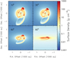 |
Fig. 1 Disc surface density extracted from the numerical simulation at a snapshot of 12 kyr, inclined to 10°, 30°, 60°, and 80°, as denoted in the panels. |
4 Synthetic observations
We shift theinclined post-processed snapshot of the model simulations at 12 kyr in both dust continuum and lines to two different distances of 800 and 2000 pc by dividing the fluxes by a factor of distance squared and adjusting the pixel resolution accordingly. The generation of the synthetic observations for ALMA and NOEMA are described in detail in the following subsections.
Details of synthetic observations.
4.1 ALMA
To create synthetic ALMA observations, we use the ALMA simulator task simalma within the Common Astronomy Software Applications (CASA) software package2 to create visibility files. The model simulations adjusted to the desired distance and in units of jansky per pixel are used as the “sky model”. The location of the sky model is set to a generic position in the southern sky, with the coordinates of the centre of the map at α(J2000) = 24h 00m 00s, δ(J2000) = −35d 00h 00s. The observed sky frequency is set to 220.679 GHz with the widths of the channels for the line cubes set to 260.3 MHz (~0.35 km s−1). We use a combination of two ALMA Cycle 5 configurations, 5–6 and 5–9, to reach a desired angular resolution of ~0.08′′. The configuration files containing the information about the distribution of the antennas were obtained within CASA (version 5.1.2-4) and were labelled “alma.cycle5.6.cfg” and “alma.cycle5.9.cfg” for configurations 5–6 and 5–9, respectively. In Cycle 5, ALMA made use of 43 antennas in the 12 m arrays. The uv-coverage of the ALMA array in configuration 5–6 has baselines in the range of 15 m–2.5 km, and in configuration 5–9 covers a range of 375 m–13.9 km. We set the integration time of the synthetic observations to 30-second intervals for a total time of 18 min in configuration 5–6 and 35 min in configuration 5–9. Figure 2 shows the uv-coverage of the synthetic observations. Thermal noise was automatically added to the observations assuming precipitable water vapour of 0.5 mm.
The images were generated in CASA using the clean task with the högbom algorithm (Högbom 1974) and a natural weighting. Considering the large number of channels in the data cubes (1400), we clean the line cubes using a circular mask spanning the extent of the input sky model to make the imaging process run faster. The images at 800 and 2000 pc have synthesised beam sizes of 0.09′′× 0.06′′, PA = 88° and 0.07′′× 0.06′′, PA = 90°, respectively. The reason for the slight increase in the size of the beam for the images at 800 pc is due to the more prominent contribution of side-lobe noise at 800 pc as the source is observed to be more extended. The synthesised beam sizes and root mean square (rms) noise values for both continuum and line observations are summarised in Table 1.
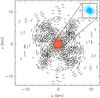 |
Fig. 2 uv-coverage of simulated ALMA observations in configuration 5–9 (in black) and configuration 5–6 (in red). The uv-coverage of simulated NOEMA observations is shown in the zoom box to the top right (in blue). |
4.2 NOEMA
For the synthetic NOEMA observations, we use the uv_fmodel task in the GILDAS3 software package developed by IRAM and Observatoire de Grenoble. To this end, we created a uv table from the input sky model by providing a uv table that specifies the desired sampling of the antennas in the uv-plane. In order to make direct comparisons to our NOEMA large program, CORE, we used the uv-coverage of our NOEMA observations in the A, B, and D arrays for source W 3(H2O) (Ahmadi et al. 2018). Six 15 m antennas were used at the time of the observations of W 3(H2O), with baselines extending the range of 19–760 m. The upper right panel of Fig. 2 shows the uv-coverage of the synthetic NOEMA observations. The integration time of the synthetic observations were made in 20-min intervals for a total time of ~11 h spread among the three different arrays. The details of the observing sequence is described in detail in Ahmadi et al. (2018). To achieve the highest possible angular resolution, we cleaned the synthetic visibilities using the MAPPING program of the GILDAS package with the clark algorithm (Clark 1980) and a uniform weighting (robust parameter of 0.1). The images have synthesised beam sizes of 0.44′′× 0.34′′, PA = 44°. The synthesised beam sizes and rms noise values for both continuum and line observations are summarised in Table 1.
5 Analysis and results
In the following, we present the continuum maps, and study the kinematics, physical conditions, and stability of the discs. We refer to the numerical simulations as “model simulations” and the synthetic ALMA and NOEMA observations accordingly.
5.1 Continuum maps
Figure 3 shows the 1.3 mm dust continuum models of the simulations at distances of 800 and 2000 pc at four different inclinations (10°, 30°, 60°, and 80°) and the corresponding synthetic ALMA and NOEMA observations. The synthesised beam sizes, linear resolutions, and rms noise values are summarised in Table 1. At this snapshot, after about 12 kyr of evolution, the fragmented accretion disc spans an extent of ~1000 au in dust continuum with four fragments seen on scales of ≤500 au, which are actively accreting material from their own smaller accretion discs (described in detail in the following section). Overdense regions connecting the fragments are a result of gravitational instabilities in the disc which had initially formed spiral arms and resulted in the creation of the fragments. The disc at this stage is still highly dynamic, with the fragments rotating about the central protostar, migrating inwards, and encountering orbital interactions and mass transfer with each other. The centre, where the protostar is actively accreting material from the disc and envelope, has a half doughnut shape as a result of the boundary conditions of the numerical simulations. The central sink has a radius of 30 au; the region within the sink is not included in the computation domain. As a result, the strongest continuum peak is the fragment found to the north-west of the protostar. The arc of material seen in the lower part of the disc shows the ejection of some material from the system. The halo seen around the disc corresponds to the envelope, which is much less dense than the disc.
The synthetic ALMA observations at 800 pc, corresponding to a linear resolution of 60 au, resolve all fragments at all inclinations. The rms noise of the continuum ALMA images at 800 au is higher than the case of the ALMA images at 2000 au as the extended nature of the structure results in more prominent side-lobe noise. Therefore, although the arc of material being ejected in the bottom is visible, it is not detected with 6σ or higher certainty. On the contrary, the synthetic ALMA observations at 2000 pc have lower side-lobe noise and therefore detect this arc with 6σ confidence. At this distance, with a linear resolution of 130 au, ALMA is able to detect all fragments, but just barely detects the closest one to the protostar, and detangling the fragments at an inclination of 80° becomes difficult. This disparity in the nature of the noise and the more prominent contribution of side-lobe noise at 800 pc is the reason why the synthesised beam at 800 pc has a slightly larger size than at 2000 pc.
The synthetic NOEMA observations at 800 pc, corresponding to a linear resolution of ~300 au, are able to resolve all the fragments at 10° and 30° inclinations, while only three are resolved at 60° inclination, and two at a near edge-on view of 80° inclination. At 2000 pc, corresponding to a linear resolution of ~800 au, only one structure is resolved regardless of the inclination. However, the structure has an elongated shape in the direction of the brightest fragment in the north-west, hinting at the possibility of unresolved fragmentation. At both distances the disc is seen to have a larger extent due to beam smearing. The angular resolution of NOEMA is expected to improve by roughly a factor of two with the expected baseline extension in the coming years. With the upgraded NOEMA, our synthetic NOEMA observations at 2000 pc will roughly resemble the presented observations at 800 pc.
5.2 Kinematics
In the following, we study the kinematics of the disc through moment analysis and PV diagrams.
5.2.1 Moment maps
We create moment maps of CH3CN (124−114) to study the disc kinematics in more detail. For the model simulations, we add arbitrary Gaussian noise to the cubes and create the moment maps with constraints on the minimum emission level set at 6σ. While there is no need to add noise to the model simulations, it makes for a cleaner presentation of the data and easier comparison with maps of the synthetic observations, and allows for the automation of the procedures with the observations. For the synthetic observations, due to the non-Gaussian nature of noise and the large contribution of side-lobe noise in the imaged cubes, we take a higher threshold of 18σ to constrain our study of the kinematics to the disc region. The range of velocities over which the moment maps have been integrated isthe same for the model simulations and the synthetic observations.
Figure 4 shows the integrated intensity (zeroth moment) map of CH3CN (124−114) for the model and synthetic observations, with continuum contour overlays. The distribution of CH3CN gas is found to be extended by a few hundred astronomical units beyond the compact dust emission, with the peaks of gas emission coinciding with dust emission peaks as expected. This extension of gas is due to the contribution of the envelope. The envelope itself is rotating and infalling onto a ring-like structure at the location of the centrifugal barrier which can best be seen in the zeroth moment maps of the 10° and 30° inclined cubes (further discussed in Sect. 5.2.2). The arc of ejected material in the bottom is also seen in the integrated intensity maps and is clearly recovered in some of the synthetic observations. The distribution of gas in the synthetic NOEMA observations at 2000 pc are more symmetrically distributed than the dust emission, which has an elongated shape. This occurs because the fraction of gas that is being accreted onto each of the fragments iscompletely washed out by the large beam, and therefore the main contribution left is the larger scale disc component that is feeding the protostar at the centre. Similarly, in the synthetic NOEMA observations at 800 pc the peak of the integrated intensity map is at the centre, whereas the dust continuum peaks at the location of the fragment to the north-west. This is because the innermost 30 au around the accreting protostar is not included in the computation domain, due to the existence of the sink particle, and is therefore not bright in the continuum observations.
Figure 5 shows the intensity-weighted peak velocity (first moment) map of CH3CN (124−114) for the numerical simulations and synthetic observations, with continuum contour overlays. The velocity gradient seen at 10° inclinations mainly showthe contribution from the infalling and rotating envelope with the edges of the envelope shell clearly visible as it has the highest velocity offset from the local standard of rest (LSR) velocity. As the structure gets more inclined, the disc contributionbecomes more clearly visible with larger velocity variation seen between the red-shifted and blue-shifted gas. The synthetic observations are able to recover the kinematics of the gas well, with the envelope and disc contributions becoming heavily blended in the poorly resolved NOEMA observations making the amplitude of the velocity gradient smaller. The Yin-Yang appearance of the first moment map is due to the fragments accreting some of the infallinggas that would have otherwise accreted onto the central protostar had the fragments not existed. This can be seen more clearly in Fig. 6, which shows zoom panels of the first moment map of CH3CN (124−114) on the positions of the fragments for the model simulations at 800 pc and inclined by 60°. The line-of-sight velocity gradient across the central protostar is in the east–west direction and has the largest amplitude as the accretion rate is highest onto the central protostar. The rotation axis of small accretion discs surrounding each of the fragments isnot necessarily inherited from the east–west rotational motion of the large-scale disc, but is set according to local dynamics. In the more inclined views towards edge-on, the Yin-Yang effect is less prominent than in the more face-on views as the fragments and their small discs are seen in one plane and start to obscure each other.
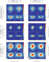 |
Fig. 3 1.37 mm continuum images of the model simulations (top row), synthetic ALMA observations (middle row), and synthetic NOEMA observations (bottom row,) shifted to a distance of 800 pc (left column) and 2000 pc (right column). Each panel contains four sub-panels corresponding to the image inclined by 10° (top left), 30° (top right), 60° (bottom left), and 80° (bottom right). The contours for the model simulations are drawn at 1, 5, 9, 20, 40, and 60% of the peak of the emission. The two outermost contours for the synthetic observations correspond to the 6σ and 12σ levels, the rest start at 30σ and increase in steps of 80σ (see Table 1 for the noise values). The synthesised beam is shown in the bottom left corner and a scale bar in the bottom right corner of each set of synthetic observations. The intensity scale is different in each panel. |
 |
Fig. 4 Integrated intensity (zeroth moment) maps of CH3CN (124−114) for the model simulations (top row), synthetic ALMA observations (middle row), and synthetic NOEMA observations (bottom row,) shifted to a distance of 800 pc (left column) and 2000 pc (right column). Each panel contains four sub-panels corresponding to the image inclined by 10° (top left), 30° (top right), 60° (bottom left), and 80° (bottom right). The contours correspond to 1.37 mm continuum as shown in Fig. 3. The synthesised beams is shown in the bottom left corner and a scale bar in the bottom right corner of each set of synthetic observations. The scale is different in each panel. |
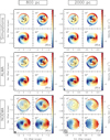 |
Fig. 5 Intensity-weighted peak velocity (first moment) maps of CH3CN (124−114) for the model simulations (top row), synthetic ALMA observations (middle row), and synthetic NOEMA observations (bottom row,) shifted to a distance of 800 pc (left column) and 2000 pc (right column). Each panel contains four sub-panels corresponding to the image inclined by 10° (top left), 30° (top right), 60° (bottom left), and 80° (bottom right). The contours correspond to 1.37 mm continuum as shown in Fig. 3. The synthesised beam is shown in the bottom left corner and a scale bar in the bottom right corner of each set of synthetic observations. |
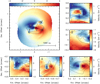 |
Fig. 6 Intensity-weighted peak velocity (first moment) map of CH3CN (124−114) for the model simulations at an inclination of 60° and shifted to a distance of 800 pc (top left). The surrounding panels show zoomed views of the kinematics of each fragment as marked by the numbers in the main panel. The contours correspond to the 1.37 mm continuum shown in Fig. 3. |
5.2.2 Position–velocity diagrams
To study the kinematics in more detail, we created PV plots for a cut in the east–west direction, perpendicular to the direction of the rotation axis. Figure 7 shows the PV plots of CH3CN (124−114) for the model simulations and synthetic observation. The PV plots of the model simulations show the effect of inclination clearly in that the inner disc contribution (r < 250 au) is not strong in the more face-on views. As the source is more inclined towards edge-on, the disc component becomes prominent, with high-velocity contributions seen very close to the central protostar. The inner disc is in clear differential rotation with a Keplerian profile  about a central object with a mass of ~10 M⊙, as depicted by the green curve. The contribution seen at r > 250 au corresponds to the region where the rotating envelope is falling onto the inner disc, which has a lower radial velocity than the infall velocity of the envelope. In recent years this transition has been observed around low-mass protostars (e.g. Sakai et al. 2014; Oya et al. 2016; Lee et al. 2017; Alves et al. 2017). These studies have found that at this position, accretion shocks lead to local heating, causing a change in the chemistry as material is liberated off the ice mantles to the gas phase. Furthermore, evidence for the centrifugal barrier around a high-mass protostellar envelope has recently been reported by Csengeri et al. (2018). This transition region is estimated to be an order of magnitude closer to the central protostar in the low-mass regime (e.g. 30–50 au for IRAS 16293–2422 Source B; Oya et al. 2018) than in the reported high-mass case (300–800 au; Csengeri et al. 2018). Our estimate of the centrifugal barrier located at r~250 au is in agreement with the lower end of the estimates from the observations of Csengeri et al. (2018).
The sharpness of this discontinuity feature seen in the PV plots is a function of resolution and inclination angle. It can be seen in the NOEMA observations at 2000 au that the “kink” seen in the other PV plots as a result of this transition is completely smoothed out. Furthermore, the velocity profile of the infalling rotating envelope would look different depending on the offset between the line of sight and the source position, as depicted in Fig. 3b of Sakai et al. (2014), which can have an effect on the sharpness of this discontinuity. The PV plots presented in this work have been made for a cut that goes through the protostar as we have knowledge of the precise location of the protostar.
The PVplots of the synthetic ALMA observations resemble the PV plots of the model simulations, but smoothed in the position direction. The high-velocity components are still clearly detected in the more inclined cases, but the spreading ofemission would mean that the Keplerian curve corresponding to rotation of matter about a ~10 M⊙ star does not perfectly fit anymore, especially in the 2000 pc case. As we move to the synthetic NOEMA observations and the emission gets even more smeared in the position direction, the high-velocity components seen in the more inclined views become hard to detect and the Keplerian curve does not fit the observations well. This is best seen in the synthetic NOEMA observations at 2000 pc where the inner disc and envelope contributions are completely blended and the resulting PV plots more closely resemble rigid-body rotation than differential rotation, similar to many observational data sets in the last decade at comparable resolutions.
As temperature is expected to be higher in regions of the disc closer to the protostar, we would expect line transitions that require higher excitation energies to be present in regions closer to the star. One signpost of differential rotation in observations is often seen in the steepening of the slope of the emission in the PV diagrams for the higher excited lines, such that a transition that is tracing the innermost regions of the disc would have higher velocities at smaller radii than the transitions that trace the entire disc region. This has been observed in the case of higher K transitions of CH3CN (Johnston et al. 2015), or vibrationally excited CH3CN transitions (Cesaroni et al. 2017). Comparing the PV plots of CH3CN (122−112) to CH3CN (124−114) and CH3CN (126−116), we do not see this steepening of the slope with higher K levels because all lines trace regions with similar optical depths and therefore probe similar regions.
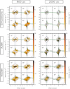 |
Fig. 7 Position–velocity plots of CH3CN (124−114) for a cut in the east–west direction across the model simulations (top row), synthetic ALMA observations (middle row), and synthetic NOEMA observations (bottom row,) shifted to a distance of 800 pc (left column) and 2000 pc (right column). Each panel contains four sub-panels corresponding to the image inclined by 10° (top left), 30° (top right), 60° (bottom left), and 80° (bottom right). The three outermost black contours correspond to the 6, 12, and 18σ levels. The remaining black contours increase in steps of 150σ. The green curves correspond to the region within which emission is expected if the gas is in a disc in Keplerian rotation about a 10 M⊙ star. The colour scale is the same for each row to show the effect of loss of emission with increasing distance. The vertical and horizontal dashed lines correspond to the position of the protostar and zero LSR velocity. The vertical dotted lines correspond to the radii at which the centrifugal barrier is seen (± 250 au). The positionresolution is shown as a scale bar in the bottom right corner of each set of synthetic observations. The velocity resolution is 0.35 km s−1 . |
5.3 Temperature distribution
To gain a better understanding of the disc structure, we calculated the rotational temperature and column density of the dense-gas tracer CH3CN under the assumption of local thermodynamical equilibrium (LTE). To do so, we used the eXtended CASA Line Analysis Software Suite (XCLASS4, Möller et al. 2017)software in CASA. In Fig. 8 we show the resulting rotational temperature maps obtained from pixel-by-pixel XCLASS modelling ofCH3CN (12K−11K) K = 4−6 for the synthetic observations. The recipe is as outlined in Appendix B of Ahmadi et al. (2018) where we discuss the reasoning behind not including the lower K-ladder transitions in the fitting routine. In these runs, we also allowed the size of the source to be a fitting parameter rather than fixing it to a value larger than the beam. This strategy was tested and it yields smoother temperature maps. For each synthetic observation,we calculated the rms noise in the emission-free region in the channel that has the peak of emission for CH3CN (124−114), and only fit pixels with signal higher than six times this noise. We note that the spectra at the positions where the envelope is directly falling onto the disc are triply peaked corresponding to red- and blue-shifted infall from the envelope onto the disc with a third component corresponding to the rotational motion of the disc itself. This is particularly prominent in the views closer to face-on. Since performing a three-component fit to the entire map was not feasible, we smoothed the velocity resolution by a factor of eight, reaching a spectral resolution of 2.8 km s−1, to blend all three components of the lines enough to perform a one-component fit to the spectrally smoothed data cubes.
Figure 8 shows the resulting rotational temperature maps for the synthetic observations. Under the LTE assumption, the rotational temperatureof CH3CN can be accepted as the kinetic temperature of the gas. The median gas temperatures obtained from the synthetic observationsat each inclination are listed in Table 2. On average, temperature decreases as the system becomes more inclined, which is expected as the observed column densities are higher in the more inclined views. In addition, the arc of material being ejected from the system seen at the bottom of the disc has a higher temperaturethan its surroundings. For comparison, the face-on view of the disc mid-plane temperature from the model simulations is presented in Fig. 9 on the same logarithmic scale. Mid-plane temperatures at the location of fragments can reach values higher than 1000 K, but on average the median temperature for the inner disc (r < 400 au) is 177 K, about 50 K warmer than the outer envelope (400 au < r < 800 au), which has a median temperature of 128 K. In Table 2 we also list median temperature values calculated for the regions within 12σ dust continuum contours (the second outermost contours in Fig. 8), which more closely correspond to the disc. On average, and as expected, the temperatures are higher in the disc than in the outer envelope. Moreover, the temperature decreases as angular resolution worsens when the disc structure is no longer recovered. Interestingly, the temperature distributions for the synthetic NOEMA observations at 2000 pc at 10° and 30° inclinations are elongated in the same direction as the continuum, while this elongation feature is not seen in the respective zeroth moment maps of CH3CN (124−114) (bottom right panel of Fig. 4).
5.4 Massestimates
At the snapshot of the numerical simulations under investigation, the protostar has gained a mass of ~10 M⊙. In the following, we describe the different techniques often used in observations for determining core and protostellar masses.
5.4.1 Masses from dust emission
Because dust opacity decreases with increasing wavelength, thermal emission of dust at longer wavelengths in the Rayleigh-Jeans limit can trace large column densities and provide estimates for the dust mass if the dust emissivity is known (Hildebrand 1983). Assuming optically thin dust emission at 1.3 mm, for a gas-to-dust mass ratio R and a dust absorption coefficient κν, we can convert the flux density Fν of the continuum observations to a mass value via
 (5)
(5)
where d is the distance to the source and Bν (TD) is the Planck function, which at the wavelengths under investigation follows the Rayleigh-Jeans law and is linearly dependent on the dust temperature TD. We adopt a value of 150 for the gas-to-dust mass ratio (Draine 2011) and κν = 0.9 cm2 g−1 corresponding to thin ice mantles after 105 yr of coagulation at a density of 106 cm−3 (Ossenkopf & Henning 1994). We assume the kinetic temperature of the gas, derived from the radiative transfer modelling of CH3CN (12K−11K) K = 4−6 (see Sect. 5.3) to be coupled to the dust temperature. Therefore, we use the temperature maps presented in Fig. 8 together with the continuum maps shown in Fig. 3 to create mass maps. Summing over all pixels, we then obtain a total mass for each synthetic observation, summarised in Table 2. The values are on average between 2.5–3.5 M⊙. For comparison, the total mass within the inner 8400 × 8400 au box for the model simulations is ~14 M⊙ calculated in the same manner by using the face-on continuum map and the mid-plane temperature shown in Fig. 9, which accounts for the total gas mass in this area. The bulk of the remaining mass is on larger scales and is not included in our analysis. Therefore, the mass estimates from the synthetic observations recover roughly 20% of the total mass calculated from the model simulations and the bulk of the flux is filtered out by the interferometer.
Considering only the synthetic ALMA observations, the mass estimates at 2000 pc are on average smaller than at 800 pc, by roughly 10%. Since the average temperature distribution does not vary significantly between the two cases, we would expect the mass estimate to also be consistent. This small excess of mass corresponds to the contribution from the halo of material found outside of the 6σ continuum contours in the middle panels of Fig. 3. Since the continuum maps at 800 pc are noisier than at 2000 pc (see Table 1) the mass estimates at 800 pc are higher than at 2000 pc. Conversely, the mass estimates at 2000 pc for the synthetic NOEMA observations are roughly 20% higher than at 800 pc. While the average temperature is not significantly different in the two cases (see Table 2), the distribution of temperatures in the innermost regions where the bulk of continuum emission is concentrated is significantly cooler in the 2000 pc case than at 800 pc (see bottom row of Fig. 8), resulting in a higher mass estimate at the greater distance.
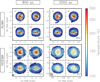 |
Fig. 8 Rotational temperature maps of synthetic ALMA observations (top row) and synthetic NOEMA observations (bottom row,) shifted to a distance of 800 pc (left column) and 2000 pc (right column), obtained by fitting CH3 CN (12K−11K) K = 4−6 lines simultaneously with XCLASS. Each panel contains four sub-panels corresponding to the image inclined by 10° (top left), 30° (top right), 60° (bottom left), and 80° (bottom right). The synthesised beam is shown in the bottom left corner of each set of synthetic observations. The contours correspond to the 1.37 mm continuum shown in Fig. 3. The scale used in the plots is for ease of comparison to the “true” disc mid-plane temperature shown in Fig. 9. |
Summary of temperatures, masses, and Q values for the synthetic observations.
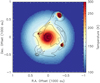 |
Fig. 9 Face-on view of the disc mid-plane temperature from the model simulations. The contours correspond to the continuum image and are drawn at 1, 5, 9, 20, 40, and 60% of the peak of the emission. The scale used in the figure is for ease of comparison to the synthetic observations shown in Fig. 8. Temperatures at the locations of the fragments get as high as 1000 K. |
5.4.2 Protostellar masses from PV plots
Protostellar masses are often estimated from fitting Keplerian profiles with  to PV diagrams. In Fig. 7 we show the PV plots for the model simulations and synthetic observations for a cut along the east–west direction going through the centre of the sink particle where the protostar is located. While the green curves correspond to the region within which emission is expected if the gas is in a disc in Keplerian rotation about a 10 M⊙ star, they do not represents fits to the PV plots. In order to estimate protostellar masses from these PV plots, we use the KeplerFit package5 (described in Bosco et al. 2019), which uses the method presented in Seifried et al. (2016). The method first identifies the two quadrants of the PV plot that contain most of the emission and then, starting from the positions closest to the protostar and moving outwards, it determines the highest velocity at which the signal becomes higher than a given threshold. This then determines the boundary which these authors call the “upper edge” of the PV plot which is then fit with a Keplerian profile to determine the enclosed mass. This method has proven to yield more accurate mass estimates than fitting the pixels with the maximum intensity for each radius or for each velocity channel (Seifried et al. 2016).
It can clearly be seen from the PV plots shown in Fig. 7 that the rotating and infalling envelope (regions outside the vertical dashed lines) shows different kinematic signatures than the inner disc, as discussed in Sect. 5.2.2. More specifically, there is a discontinuity in the resolved PV plots as a result of the infalling and rotating envelope having a higher infall velocity than the inner disc. Therefore, fits to the inner regions would be expected to yield lower mass estimates than to the outer envelope, which at a given position has higher velocities. For this reason we fit the inner and outer part of the disc separately and compare the results to the case where the entire PV diagram is fitted. An example is shown in Fig. 10 for the model simulations at 800 pc. We always fit the 6σ outer edge for a range of radii and always exclude in the fitting the regions closest to the protostar where the velocity decreases with decreasing distance to the protostar as a result of finite resolution (see Appendix A.3.2 of Bosco et al. 2019). The resulting mass estimates from fitting the inner, outer, and entire PV curves for the model simulations and synthetic observations are presented in Fig. 11. Knowing that the central protostar has gained a mass of ~10 M⊙ and that the disc mass is ~8 M⊙ at this snapshot of the simulation, we can test the accuracy of estimating the enclosed masses using this method in each scenario. We first focus on the general findings.
As rotational velocity is expected to scale with inclination angle i by a factor of sin (i), the mass estimates are expected to scale by a factor of sin2 (i). Therefore, it is expected that fitting the kinematics of the more inclined discs would result in higher mass estimates than their less inclined counterparts (grey curves in Fig. 11). While this general trend is seen in our fitting results, we find that the fitted masses are on average higher than the theoretical expectation, similar to the findings of Seifried et al. (2016). For example, we would expect the enclosed mass estimate at 30° to be 0.25 times lower than the true value of 18 M⊙ at 90° inclination; however, the mass estimate from the fitting the inner region of the model simulation is higher than the expected 4.5 M⊙ by 35%. Seifried et al. (2016) attribute this increase to the existence of considerable radial motions, which in the more inclined views noticeably contributes to the line-of-sight velocities. It is worth noting that while the 10 M⊙ protostar is located at the centre of the computational domain at zero offset in the PV diagrams, the disc which contains roughly 8 M⊙ spans a range of radii, such that the mass-velocity relation is  . Therefore, the enclosed mass is not exactly 18 M⊙ at all radiiand the true theoretical curve lies somewhere between the solid and dashed lines in Fig. 11. Interestingly, the fits to the inner disc of the model simulations inclined to 60° and 80° provide mass estimates in this range.
For the model simulations where we fit the PV curves of the model simulations and the ALMA observations at 800 pc, the protostellar mass estimates obtained from fitting the inner disc regions are, as expected, smaller than the estimates from fitting the outer or entire regions, and provide estimates closer to the expected values. For these cases, fits tothe entire region yield masses that are less than the mass estimates obtained from fitting the outer regions. In these cases, fits to the outer regions overestimate the masses because the component that is fitted is mainly the envelope within which more mass is contained and which does not necessarily have a Keplerian rotation profile.
For all observations, the method overestimates the mass, even when fitting the inner disc regions. The mass is much more overestimated for discs with lower inclinations (i.e. views closer to face-on). The fact that we generally overestimate the masses especially at lower inclinations can be seen as favourable since without knowing the inclination in most observations, the mass estimate obtained from fitting the PV diagram is typically adopted as the protostellar mass without any corrections for inclination. Therefore, it is somewhat reassuring that fits to the entire region for the model simulations and all ALMA observations, which properly resolve the disc, are quite close to the expected enclosed mass of ~18 M⊙ at all inclinations.
As resolution worsens, in the case of the synthetic ALMA observations at 2000 pc and synthetic NOEMA observations at both distances, the fits to the outer regions provide the lowest mass estimates, which are also closer to the expected value. For the ALMA observations, the variations in the mass estimates from fits to different regions are not as significant as for the NOEMA observations at 800 and 2000 pc, where the fits to the inner regions can yield masses that are larger than the fits to the outer regions by almost a factor of 2 and 4, respectively.
While the Seifried et al. (2016) method of fitting the outer edge of the PV diagram used to determine the enclosed mass is the most accurate method currently used, we find that fitting the entire PV diagram of poorly resolved observations yields masses that are highly overestimated. This is expected as the emission is smeared over a larger area with the envelope and disc components completely blended, resulting in the PV diagrams not having a Keplerian shape (see bottom row of Fig. 7). In these cases, we find that fitting the outer regions of the PV diagram (in our cases, regions beyond 1600 au) provides better estimates for the protostellar mass. The same analysis was done for the PV plots of CH3CN (12K−11K), K = 3, 5, 6 lines, and the variations in the mass estimates were marginal compared with those presented in Fig. 11 for the K = 4 transition. The only noticeable difference was that the mass estimates obtained from fitting the PV diagrams of the K = 3 transition were slightly higher than those obtained from the other lines as this transition is more easily excited than the others and the emission is hence distributed over a larger area.
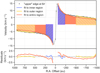 |
Fig. 10 Example of the Keplerian fitting approach based on Seifried et al. (2016) to the 6σ outer edge of the PV plot of CH3CN (124−114) for the model simulation inclined to 60° at a distance of 800 pc in order to determine the protostellar mass. The fits to the inner, outer, and entire regions yield protostellar mass estimates of 12.4, 21.4, and 15.4 M⊙, respectively. The inner region traces the disc that follows a Keplerian rotation curve better than the outer region, which has contributions from the rotating and infalling envelope. The bottom panel shows the residuals. The protostar has a mass of ~10 M⊙ while the disc has a mass of ~8 M⊙ . |
5.5 Toomre stability
As mentioned in the Introduction, the Toomre Q parameter can be used to study the stability of a disc against gravitational collapse (Toomre 1964). The stabilising force of gas pressure is included in the expression of Q (Eq. (1)) via the sound speed,
 (6)
(6)
where γ is the adiabatic index with a value of 7∕5 for diatomic gas, kB is the Boltzmann constant, μ is the mean molecular weight with a value of 2.8, and mH is the mass of the hydrogen atom. Furthermore, we account for the stabilising force of shear by assuming the disc is in Keplerian-like rotation such that the angular velocity of the disc at a given radius r would be
 (7)
(7)
In Fig. 12 we show the “true” Q map obtained from the model simulations. As expected, we see low Q values at the positions of the fragments since these regions have already collapsed to form protostars; we also see low Q values in a ring coincident with the edge of the disc. Since the mid-plane temperature decreases smoothly towards the edges of the disc (see Fig. 9), we would expect a decrease in the Q parameter in the outskirts of the disc, butthe existence of low Q values in a ring-like structure is due to enhanced disc surface density in a ring of material in this region (see Fig. 1). It is important to note that the Toomre analysis is meaningless outside of the disc region; therefore, the transition from stable (high Q) on envelope scales to unstable (low Q) at larger radii in the outskirts of the maps has no physical meaning. This transition is best seen inthe view closest to edge-on in Fig. 12 at a declination offset of about ± 800 au.
In the following, we estimate the distribution of Q for the synthetic observations and start the analysis by adopting the known protostellar mass at this snapshot and correcting the angular velocities for the known inclinations. The effects of not correcting the velocities properly and uncertainties in mass estimates are further discussed in Sects. 5.5.1 and 5.5.2, respectively. We assume thatthe LTE assumption is valid in such a high-density environment, and use the rotational temperature of CH3CN modelled in Sect. 5.3 as representative of the kinetic temperature of the gas. To account for the self-gravity of the disc, we include the mass of the disc within a given radius (Mdisc(r)) to the mass of the protostar M* assumed to be 10 M⊙. The angular velocity is further corrected to account for the inclination of the disc such that
 (8)
(8)
In particular, the radius at each pixel in a face-on disc is calculated as  , where Δx is the distance from the protostar in right ascension and Δy is the distance from the protostar in declination. Since we do not rotate the structure, but only incline it about the x-axis, the projected radius is
  .
.
The mass of the disc is calculated as discussed in Sect. 5.4.1 from the continuum emission maps by summing up the mass contained within each projected radius using the aperture photometry tools of the photutils package (Bradley et al. 2016) within the astropy package (Astropy Collaboration 2013) in Python. Furthermore, the beam-averaged surface density of the disc is calculated via
 (9)
(9)
where Sν is the peak intensity and ΩB is the beam solid angle.
In Fig. 13, we show the Q maps for the synthetic observations. Again, as expected, we find low Q values below the critical value of 1 at the positions of the fragments in the synthetic observations which resolve them. This is attributed to the enhanced surface density at the positions of the fragments that have already collapsed to form stars. We also find low Q values (~1–2) in the arms connecting the fragments, as well as the arc of material to the south being expelled from the system. The arms connecting the fragments can be locations where further disc fragmentation can take place. The extremely low Q values above and below where the continuum contours are drawn in the view closest to edge-on (80°) are a result of lowangular velocities at these positions since the disc only extends a small distance in declination. The gas contribution at these locations comes from the rotating and infalling envelope, and the Toomre analysis is actually not applicable for this envelope medium.
The ring of low Q values seen in the model simulations (see Fig. 12) is not seen in the Toomre maps of the synthetic observations. Since the produced dust continuum images are essentially a convolution of the temperature with the density, the radial decrease in temperature in the outskirts (see Fig. 9) where the ring exists in the density (see Fig. 1) results in this component not being prominent in the final continuum images (see Fig. 3). Therefore, because we use the continuum maps to calculate the surface density of the discs in the Toomre equation, this component is also non-existent. Interestingly, we find high Q values in a ring just outside of the lowest continuum contours, best seen in the synthetic ALMA observations inclined 10° and 30°. This is a result of high gas temperatures in these regions, due to shock heating of gas falling from the rotating envelope onto the disc.
The synthetic NOEMA observations at 800 pc still show low Q values at the positions of the fragments, but the low values expected to be seen in the arms connecting the fragments are absent because the temperature distribution is uniform in the inner regions (see bottom left panel of Fig. 8). Most interestingly, although the synthetic NOEMA observations at 2000 pc do not resolve the individual fragments, we find low Q values ~2 in the outskirts of the disc. This is a result of the structure having a non-circular elongated shape in the direction of the brightest fragment in the north-west in both the continuum and temperature distributions.
The critical value of Q is often taken to be 1 in theoretical calculations, and lowers to ~0.7 for an isothermal disc of finite thickness (Goldreich & Lynden-Bell 1965; Gammie 2001). Considering that our modelling of the level populations of the CH3CN K-ladder provides gas temperatures that may probe layers above the disc mid-plane, we assume that regions where Q is less than ~2 are unstable against gravitational collapse. The median Q values are listed in Table 2 and follow a trend opposite to that of the mass estimates; the Toomre parameter is inversely proportional to the surface density of the disc, which is calculated in a manner similar to that used for the mass estimates but without the distance dependence.
At first glance we see that, on average, the Q parameter gets lower with increasing inclination. This is naively expected as in the edge-on views one looks through a larger column. To investigate the effect of inclination further in the resolved observations, the histogram of Q values for synthetic ALMA observations at 2000 pc is shown as an example in the top panels of Fig. 14. We attempt to remove as much of the contribution as possible from the envelope by only plotting the histogram of Q values for the pixels that lie within 6σ continuum contours, which are the outermost contours drawn on the maps in Fig. 13. The Q distributions in these inner regions do not vary much for the 10°, 30°, and 60° views, but still a large portion of the contribution for the 80° inclined map comes from the envelope since the disc contribution is just a narrow region spanning a few pixels in declination. The angular velocities in the envelope for the case closest to edge-on are low and therefore result in low Q values there. For comparison, in the bottom panel of Fig. 14 we show the histogram of Q values for the inclined models where only pixels within a radius of 1600 au are included in order to exclude the meaningless contribution from the larger scale cloud. While the distribution is broader, as there are more pixels with low Q values for each fragment, the findings remain the same.
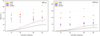 |
Fig. 11 Massestimates from fitting the 6σ edges of the PV diagrams of CH3CN (124−114) shown in Fig. 7 using the method introduced by Seifried et al. (2016) for the model simulations (yellow), ALMA (purple), and NOEMA observations (orange) at 800 pc (left) and 2000 pc (right). The triangles pointing to the left and right correspond to fits to the inner and outer regions, respectively. The diamonds correspond to fits to the entire PV curves. The transparency of the markers correspond to the χ2 value of the fit, weighted by the χ2 value of the best-fit curve for a given region. The more opaque the marker, the better the fit. The solidand dashed grey curves correspond to the true estimate for the mass of the protostar (10 M⊙), and the mass of the protostar + disc (18 M⊙), respectively, corrected by sin2 (i) for each inclination i. |
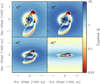 |
Fig. 12 True Q map obtained from the model simulations inclined by 10° (top left), 30° (top right), 60° (bottom left), and 80° (bottom right). The contours correspond to 1.37 mm continuum as shown in Fig. 3. Q values of less than 1 correspond to regions unstable against gravitational collapse. |
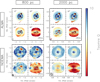 |
Fig. 13 Toomre Q map of synthetic ALMA observations (top row) and synthetic NOEMA observations (bottom row,) shifted to a distance of 800 pc (left column) and 2000 pc (right column). Each panel contains four sub-panels corresponding to the image inclined by 10° (top left), 30° (top right), 60° (bottom left), and 80° (bottom right). In each case, the disc is assumed to be in Keplerian rotation about a 10 M⊙ star at the centre. The angular velocities have been corrected for the inclination (see text). The contours correspond to the 1.37 mm continuum shown in Fig. 3. The synthesised beam is shown in the bottom left corner and a scale bar in the bottom right corner of each set of synthetic observations. Q values of less than 1 correspond to regions unstable against gravitational collapse. |
5.5.1 Inclination of the angular velocity field
In true observations, we seldom have information about the inclination of the source. Sometimes the outflow geometry can help, but high-mass stars form in highly clustered environments, and with the outflow angles widening with time (Beuther & Shepherd 2005) there is a very good chance that outflows emanating from different sources may overlap, making the deduction of an inclination angle for the disc difficult. To check how the lack of knowledge about the inclination of the disc would affect our analysis, we produced an angular velocity map where at each pixel  , which essentially means we assume the angular velocity at each position is what it would be if the disc was edge-on in that direction.
Figure 15 shows the Q maps for the synthetic observations without the inclination correction. In the resolved ALMA observations at both distances and NOEMA observations at 800 pc, we still find low Q values, as expected, at the positions of the fragments, but the higher inclined views show higher Q values at the locations of the fragments than in the inclination-corrected cases, precisely because the angular velocities at a given point above and below the zero declination line are higher in the uncorrected maps. Interestingly, in the synthetic NOEMA observations at 2000 pc where the fragments are not resolved, we still see the low Q values in the outskirts of the structure. Therefore, the conclusion from the corrected case still holds that we are able to predict fragmentation of the disc without actually resolving the fragments.
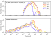 |
Fig. 14 Top: histogram of Q values for synthetic ALMA observations at 2000 pc (see top right panel of Fig. 13), including only pixels that lie within 6σ continuum contours to show the Q distribution mostly associated with the disc rather than the envelope. Bottom: histogram of Q values for model simulations (see Fig. 12), including only pixels within a radius of 1600 au. |
5.5.2 Uncertainties in the mass of the central object
In our Toomre analysis, we have assumed the mass of the protostar at the centre to be 10 M⊙ as we have access to this information. In Sect. 5.4.2 we outlined how the mass of the central object is often estimated from the kinematics of the disc, and explained that with loss of resolution, the shape of the rotation curve of the disc changes from differential to a more rigid-body appearance. Therefore, fitting Keplerian curves to the PV plots of poorly resolved structures would overestimate the mass of the central object. Since the mass of the protostar has a square root dependence in the expression of Q (Eq. (1)), overestimating the protostellar mass by a factor of 4 would yield Q values that are on average higher by a factor of two, making the discs seem more stable.
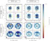 |
Fig. 15 Same as Fig. 13, but assuming the inclination of the object is not known, and therefore with the velocities not corrected to the actual rotation velocities. |
6 Summary and conclusions
In this work, we have presented synthetic ALMA and NOEMA observations for a high-resolution 3D radiation-hydrodynamic simulation of a high-mass protostellar disc that fragments into a highly dynamic system. At the snapshot of the simulation at 12 kyr, the system comprises a central protostar and four companion fragments on scales ≤500 au, all accretingmaterial from the infalling and rotating envelope that feeds the disc that is in Keplerian rotation. Smaller accretion discs are formed around each of the fragments, through which some of the large-scale disc and envelope material is accreted onto the fragments. The aim of the investigation has been to study the effect of inclination and spatial resolution in recovering disc structure and to study the stability of the disc in order to predict disc fragmentation and better understand recent and future high-resolution observations. The following is a summary of our findings:
-
Synthetic ALMA observation at 800 pc are able to detect all fragments at all inclinations in both continuum and line emission at 1.3 mm. At 2000 pc, the ALMA observations at 80° inclination cannot resolve the closest fragment to the protostar. The NOEMA observations at 800 pc can resolve all fragments at 10° and 30° inclinations, but not all at higher inclinations. At 2000 pc, NOEMA observations only show a single structure that looks slightly elongated towards the brightest fragment.
-
In the zeroth moment maps of CH3CN (12–11) rotational transitions, the peak of emission is at the position of the protostar. For the ALMA observations at both 800 and 2000 pc, we are able to detect the rotating envelope that is infalling onto a ring-like structure at the position of the centrifugal barrier. The effect is best seen in the 10° and 30° inclined views.
-
In the first moment maps of CH3CN (12–11) rotational transitions the disc contribution is best seen in the higher inclined views, as expected. There are small accretion discs around each fragment feeding them part of the disc material; this leads to the large-scale velocity field of the disc having a Yin-Yang shape. Envelope and disc contributions are heavily blended in the poorly resolved case of NOEMA observations at 2000 pc (linear resolutions ~800 au) where the emission is also smeared over a larger distance, making the amplitude of the observed velocity gradient smaller.
-
PV diagrams of CH3CN (12–11) rotational transitions for a cut through the disc perpendicular to its rotation axis show the differential (Keplerian) rotation of material best in the close to edge-on view. At a radius of ~250 au a discontinuity is seen, corresponding to the position of the centrifugal barrier because the infalling envelope has a higher infalling velocity than the radial velocity of the disc. As the entire structure becomes less resolved in the NOEMA observations, the high-velocity components of the disc become washed out and blended with the envelope component, making the PV diagrams resemble rigid-body rotation.
-
We fit the emission of CH3CN (12K−11K) K = 4−6 with XCLASS to obtain rotational temperature maps for the discs. On average we find temperatures in the range of 100–300 K, decreasing as the system becomes more inclined. The envelope is roughly a factor of 2 cooler than the disc. In the poorly resolved NOEMA observations, the envelope and inner disc contributions become blended and the difference between the temperature of the inner and outer regions is not as apparent as in the resolved cases.
-
Assuming gas and dust temperatures are coupled, mass estimates from dust for the synthetic observations account for roughly 20% of the mass calculated from the model simulations for the inner 8400 × 8400 au, and the rest is filtered out by the interferometers.
-
We make use of the method presented in Seifried et al. (2016) to fit the PV plots with Keplerian models to obtain protostellar mass estimates. Since there is a discontinuity in the 6σ outer edge of the PV plots as a result of material falling from the envelope onto the disc, we fit the inner disc and outer envelope regions separately. In the case of well-resolved discs with Keplerian profiles, we find the fits to the inner regions the most accurate and the fits to the entire PV curves adequate for estimating enclosed masses. For poorly resolved discs, the fits to the outer regions of the PV diagrams yield much more accurate mass estimates as opposed to fits to the entire region which overestimate the mass. The factor by which the mass is overestimated depends on how poorly the disc is resolved.
-
Studying the Toomre stability of the discs, we find low Q values below the critical value for stability against gravitational collapse at the positions of the fragments and in the arms connecting the fragments for the resolved synthetic ALMA observations. For the synthetic NOEMA observations at 800 pc (linear resolutions ~300 au), low Q values are seen at the locations of the fragments, but the unstable region in the disc is no longer seen since the temperature structure is uniformly warm for the inner disc. For the NOEMA observations at 2000 pc (linear resolutions ~800 au) where only one structure is resolved, we find low Q values in the outskirts of the disc. This is an important result as it implies that despite the lack of ability in resolving any of the fragments, we are able to predict that the disc is unstable and fragmenting.
-
Assuming that the inclination of the disc is not known, recalculating the Q maps using Keplerian velocities of an edge-on disc to all radial directions for all inclinations provide slightly higher values for the Q parameter, but the conclusions from the previous point still hold. This is reassuring as disc inclinations are difficult to establish.
In this work, we showcased the potential and limitations of studying discs in high-mass star formation with current (millimetre) interferometers. We benchmarked a method for studying the stability of such discs, showing that even with poorly resolved observations it is possible to predict whether a disc is prone to fragmentation. We aim to apply our methods to the study of a large sample of high-mass disc candidates within the IRAM large programme CORE in an upcoming paper.
Acknowledgements
We thank the anonymous referee for providing detailed comments on the manuscript which helped with the clarity and quality of the work. A.A. and H.B. acknowledge support from the European Research Council under the European Community’s Horizon 2020 framework programme (2014–2020) via the ERC Consolidator Grant “From Cloud to Star Formation (CSF)” (project number 648505). R.K. acknowledges financial support via the Emmy Noether Research Group on Accretion Flows and Feedback in Realistic Models of Massive Star Formation funded by the German Research Foundation (DFG) under grant no. KU 2849/3-1 and KU 2849/3-2.
References
- Ahmadi, A., Beuther, H., Mottram, J. C., et al. 2018, A&A, 618, A46 [NASA ADS] [CrossRef] [EDP Sciences] [Google Scholar]
- Alves, F. O., Girart, J. M., Caselli, P., et al. 2017, A&A, 603, L3 [NASA ADS] [CrossRef] [EDP Sciences] [Google Scholar]
- Astropy Collaboration (Robitaille, T. P., et al.) 2013, A&A, 558, A33 [NASA ADS] [CrossRef] [EDP Sciences] [Google Scholar]
- Banerjee, R., & Pudritz, R. E. 2008, ASP Conf. Ser., 387, 216 [NASA ADS] [Google Scholar]
- Beltrán, M. T., & de Wit, W. J. 2016, A&ARv, 24, 6 [NASA ADS] [CrossRef] [Google Scholar]
- Beuther, H., & Shepherd, D. 2005, Astrophys. Space Sci. Lib., 324, 105 [NASA ADS] [CrossRef] [Google Scholar]
- Beuther, H., Schilke, P., Gueth, F., et al. 2002, A&A, 387, 931 [NASA ADS] [CrossRef] [EDP Sciences] [Google Scholar]
- Beuther, H., Mottram, J. C., Ahmadi, A., et al. 2018, A&A, 617, A100 [NASA ADS] [CrossRef] [EDP Sciences] [Google Scholar]
- Bhandare, A., Kuiper, R., Henning, T., et al. 2018, A&A, 618, A95 [NASA ADS] [CrossRef] [EDP Sciences] [Google Scholar]
- Bosco, F., Beuther, H., Ahmadi, A., et al. 2019, A&A, 629, A10 [NASA ADS] [CrossRef] [EDP Sciences] [Google Scholar]
- Bradley, L., Sipocz, B., Robitaille, T., et al. 2016, Astrophysics Source Code Library [record ascl:1609.011] [Google Scholar]
- Cesaroni, R., Sánchez-Monge, Á., Beltrán, M. T., et al. 2017, A&A, 602, A59 [NASA ADS] [CrossRef] [EDP Sciences] [Google Scholar]
- Chabrier, G. 2003, PASP, 115, 763 [NASA ADS] [CrossRef] [Google Scholar]
- Chen, H.-R. V., Keto, E., Zhang, Q., et al. 2016, ApJ, 823, 125 [NASA ADS] [CrossRef] [Google Scholar]
- Chini, R., Hoffmeister, V. H., Nasseri, A., Stahl, O., & Zinnecker, H. 2012, MNRAS, 424, 1925 [NASA ADS] [CrossRef] [Google Scholar]
- Clark, B. G. 1980, A&A, 89, 377 [NASA ADS] [Google Scholar]
- Collings, M. P., Anderson, M. A., Chen, R., et al. 2004, MNRAS, 354, 1133 [NASA ADS] [CrossRef] [Google Scholar]
- Commerçon, B., Teyssier, R., Audit, E., Hennebelle, P., & Chabrier, G. 2011, A&A, 529, A35 [NASA ADS] [CrossRef] [EDP Sciences] [Google Scholar]
- Courant, R., Friedrichs, K., & Lewy, H. 1967, IBM J. Res. Dev., 11, 215 [NASA ADS] [CrossRef] [Google Scholar]
- Csengeri, T., Bontemps, S., Wyrowski, F., et al. 2018, A&A, 617, A89 [NASA ADS] [CrossRef] [EDP Sciences] [Google Scholar]
- Draine, B. T. 2011, Physics of the Interstellar and Intergalactic Medium (Princeton: Princeton University Press) [Google Scholar]
- Dullemond, C. P., Juhasz, A., Pohl, A., et al. 2012, Astrophysics Source Code Library [record ascl:1202.015] [Google Scholar]
- Fallscheer, C., Beuther, H., Zhang, Q., Keto, E., & Sridharan, T. K. 2009, A&A, 504, 127 [NASA ADS] [CrossRef] [EDP Sciences] [Google Scholar]
- Frank, A., Ray, T. P., Cabrit, S., et al. 2014, in Protostars and Planets VI, eds. H. Beuther, R. Klessen, C. Dullemond, & T. Henning (Tucson: University of Arizona Press) 451 [Google Scholar]
- Gammie, C. F. 2001, ApJ, 553, 174 [NASA ADS] [CrossRef] [Google Scholar]
- Gerner, T., Beuther, H., Semenov, D., et al. 2014, A&A, 563, A97 [NASA ADS] [CrossRef] [EDP Sciences] [Google Scholar]
- Goldreich, P., & Lynden-Bell, D. 1965, MNRAS, 130, 125 [NASA ADS] [CrossRef] [Google Scholar]
- Harries, T. J., Douglas, T. A., & Ali, A. 2017, MNRAS, 471, 4111 [NASA ADS] [CrossRef] [Google Scholar]
- Haworth, T. J., Glover, S. C. O., Koepferl, C. M., Bisbas, T. G., & Dale, J. E. 2018, New Astron. Rev., 82, 1 [Google Scholar]
- Hildebrand, R. H. 1983, QJRAS, 24, 267 [NASA ADS] [Google Scholar]
- Högbom, J. A. 1974, A&AS, 15, 417 [Google Scholar]
- Hosokawa, T., & Omukai, K. 2009, ApJ, 691, 823 [NASA ADS] [CrossRef] [Google Scholar]
- Ilee, J. D., Cyganowski, C. J., Nazari, P., et al. 2016, MNRAS, 462, 4386 [NASA ADS] [CrossRef] [Google Scholar]
- Ilee, J. D., Cyganowski, C. J., Brogan, C. L., et al. 2018, ApJ, 869, L24 [NASA ADS] [CrossRef] [Google Scholar]
- Jankovic, M. R., Haworth, T. J., Ilee, J. D., et al. 2019, MNRAS, 482, 4673 [NASA ADS] [CrossRef] [Google Scholar]
- Johnston, K. G., Robitaille, T. P., Beuther, H., et al. 2015, ApJ, 813, L19 [NASA ADS] [CrossRef] [Google Scholar]
- Kahn, F. D. 1974, A&A, 37, 149 [NASA ADS] [Google Scholar]
- Klassen, M., Pudritz, R. E., Kuiper, R., Peters, T., & Banerjee, R. 2016, ApJ, 823, 28 [NASA ADS] [CrossRef] [Google Scholar]
- Kölligan, A., & Kuiper, R. 2018, A&A, 620, A182 [NASA ADS] [CrossRef] [EDP Sciences] [Google Scholar]
- Kratter, K. M., & Matzner, C. D. 2006, MNRAS, 373, 1563 [NASA ADS] [CrossRef] [Google Scholar]
- Kratter, K. M., Matzner, C. D., Krumholz, M. R., & Klein, R. I. 2010, ApJ, 708, 1585 [NASA ADS] [CrossRef] [Google Scholar]
- Kroupa, P. 2001, MNRAS, 322, 231 [NASA ADS] [CrossRef] [Google Scholar]
- Krumholz, M. R., Klein, R. I., & McKee, C. F. 2007, ApJ, 665, 478 [NASA ADS] [CrossRef] [Google Scholar]
- Krumholz, M. R., Klein, R. I., McKee, C. F., Offner, S. S. R., & Cunningham, A. J. 2009, Science, 323, 754 [NASA ADS] [CrossRef] [PubMed] [Google Scholar]
- Kuiper, R., & Hosokawa, T. 2018, A&A, 616, A101 [NASA ADS] [CrossRef] [EDP Sciences] [Google Scholar]
- Kuiper, R., & Klessen, R. S. 2013, A&A, 555, A7 [NASA ADS] [CrossRef] [EDP Sciences] [Google Scholar]
- Kuiper, R., & Yorke, H. W. 2013, ApJ, 772, 61 [NASA ADS] [CrossRef] [Google Scholar]
- Kuiper, R., Klahr, H., Beuther, H., & Henning, T. 2010a, ApJ, 722, 1556 [CrossRef] [Google Scholar]
- Kuiper, R., Klahr, H., Dullemond, C., Kley, W., & Henning, T. 2010b, A&A, 511, A81 [NASA ADS] [CrossRef] [EDP Sciences] [Google Scholar]
- Kuiper, R., Klahr, H., Beuther, H., & Henning, T. 2011, ApJ, 732, 20 [NASA ADS] [CrossRef] [Google Scholar]
- Kuiper, R., Yorke, H. W., & Turner, N. J. 2015, ApJ, 800, 86 [NASA ADS] [CrossRef] [Google Scholar]
- Kuiper, R., Turner, N. J., & Yorke, H. W. 2016, ApJ, 832, 40 [NASA ADS] [CrossRef] [Google Scholar]
- Laor, A., & Draine, B. T. 1993, ApJ, 402, 441 [NASA ADS] [CrossRef] [Google Scholar]
- Larson, R. B., & Starrfield, S. 1971, A&A, 13, 190 [NASA ADS] [Google Scholar]
- Lee, C.-F., Ho, P. T. P., Li, Z.-Y., et al. 2017, Nat. Astron., 1, 0152 [NASA ADS] [CrossRef] [Google Scholar]
- Leurini, S., Codella, C., Zapata, L., et al. 2011, A&A, 530, A12 [NASA ADS] [CrossRef] [EDP Sciences] [Google Scholar]
- Maud, L. T., Moore, T. J. T., Lumsden, S. L., et al. 2015, MNRAS, 453, 645 [NASA ADS] [CrossRef] [Google Scholar]
- Maud, L. T., Cesaroni, R., Kumar, M. S. N., et al. 2018, A&A, 620, A31 [NASA ADS] [CrossRef] [EDP Sciences] [Google Scholar]
- Maud, L. T., Cesaroni, R., Kumar, M. S. N., et al. 2019, A&A, 627, L6 [NASA ADS] [CrossRef] [EDP Sciences] [Google Scholar]
- Meyer, D. M.-A., Vorobyov, E. I., Kuiper, R., & Kley, W. 2017, MNRAS, 464, L90 [NASA ADS] [CrossRef] [Google Scholar]
- Meyer, D. M. A., Kuiper, R., Kley, W., Johnston, K. G., & Vorobyov, E. 2018, MNRAS, 473, 3615 [NASA ADS] [CrossRef] [Google Scholar]
- Mignone, A., Bodo, G., Massaglia, S., et al. 2007, ApJS, 170, 228 [Google Scholar]
- Mignone, A., Zanni, C., Tzeferacos, P., et al. 2012, ApJS, 198, 7 [Google Scholar]
- Möller, T., Endres, C., & Schilke, P. 2017, A&A, 598, A7 [NASA ADS] [CrossRef] [EDP Sciences] [Google Scholar]
- Motte, F., Bontemps, S., & Louvet, F. 2018, ARA&A, 56, 41 [NASA ADS] [CrossRef] [Google Scholar]
- Nakano, T. 1989, ApJ, 345, 464 [NASA ADS] [CrossRef] [Google Scholar]
- Ossenkopf, V.,& Henning, T. 1994, A&A, 291, 943 [NASA ADS] [Google Scholar]
- Oya, Y., Sakai, N., López-Sepulcre, A., et al. 2016, ApJ, 824, 88 [NASA ADS] [CrossRef] [Google Scholar]
- Oya, Y., Moriwaki, K., Onishi, S., et al. 2018, ApJ, 854, 96 [NASA ADS] [CrossRef] [Google Scholar]
- Palla, F., & Stahler, S. W. 1993, ApJ, 418, 414 [NASA ADS] [CrossRef] [Google Scholar]
- Pudritz, R. E., Ouyed, R., Fendt, C., & Brandenburg, A. 2007, in Protostars and Planets V, eds. B. Reipurth, D. Jewitt, & K. Keil (Tucson: University of Arizona Press), 277 [Google Scholar]
- Rosen, A. L., Krumholz, M. R., McKee, C. F., & Klein, R. I. 2016, MNRAS, 463, 2553 [NASA ADS] [CrossRef] [Google Scholar]
- Safronov, V. S. 1960, Annales d’Astrophysique, 23, 979 [NASA ADS] [Google Scholar]
- Sakai, N., Sakai, T., Hirota, T., et al. 2014, Nature, 507, 78 [NASA ADS] [CrossRef] [Google Scholar]
- Sanna, A., Kölligan, A., Moscadelli, L., et al. 2019, A&A, 623, A77 [NASA ADS] [CrossRef] [EDP Sciences] [Google Scholar]
- Seifried, D., Sánchez-Monge, Á., Walch, S., & Banerjee, R. 2016, MNRAS, 459, 1892 [Google Scholar]
- Toomre, A. 1964, ApJ, 139, 1217 [Google Scholar]
- Wolfire, M. G., & Cassinelli, J. P. 1987, ApJ, 319, 850 [NASA ADS] [CrossRef] [Google Scholar]
- Yorke, H. W., & Sonnhalter, C. 2002, ApJ, 569, 846 [NASA ADS] [CrossRef] [Google Scholar]
- Zapata, L. A., Palau, A., Galván-Madrid, R., et al. 2015, MNRAS, 447, 1826 [NASA ADS] [CrossRef] [Google Scholar]
- Zapata, L. A., Garay, G., Palau, A., et al. 2019, ApJ, 872, 176 [NASA ADS] [CrossRef] [Google Scholar]
Developed by Felix Bosco, available at https://github.com/felixbosco/KeplerFit.
All Tables
All Figures
|
Fig. 1 Disc surface density extracted from the numerical simulation at a snapshot of 12 kyr, inclined to 10°, 30°, 60°, and 80°, as denoted in the panels. |
| In the text | |
|
Fig. 2 uv-coverage of simulated ALMA observations in configuration 5–9 (in black) and configuration 5–6 (in red). The uv-coverage of simulated NOEMA observations is shown in the zoom box to the top right (in blue). |
| In the text | |
|
Fig. 3 1.37 mm continuum images of the model simulations (top row), synthetic ALMA observations (middle row), and synthetic NOEMA observations (bottom row,) shifted to a distance of 800 pc (left column) and 2000 pc (right column). Each panel contains four sub-panels corresponding to the image inclined by 10° (top left), 30° (top right), 60° (bottom left), and 80° (bottom right). The contours for the model simulations are drawn at 1, 5, 9, 20, 40, and 60% of the peak of the emission. The two outermost contours for the synthetic observations correspond to the 6σ and 12σ levels, the rest start at 30σ and increase in steps of 80σ (see Table 1 for the noise values). The synthesised beam is shown in the bottom left corner and a scale bar in the bottom right corner of each set of synthetic observations. The intensity scale is different in each panel. |
| In the text | |
|
Fig. 4 Integrated intensity (zeroth moment) maps of CH3CN (124−114) for the model simulations (top row), synthetic ALMA observations (middle row), and synthetic NOEMA observations (bottom row,) shifted to a distance of 800 pc (left column) and 2000 pc (right column). Each panel contains four sub-panels corresponding to the image inclined by 10° (top left), 30° (top right), 60° (bottom left), and 80° (bottom right). The contours correspond to 1.37 mm continuum as shown in Fig. 3. The synthesised beams is shown in the bottom left corner and a scale bar in the bottom right corner of each set of synthetic observations. The scale is different in each panel. |
| In the text | |
|
Fig. 5 Intensity-weighted peak velocity (first moment) maps of CH3CN (124−114) for the model simulations (top row), synthetic ALMA observations (middle row), and synthetic NOEMA observations (bottom row,) shifted to a distance of 800 pc (left column) and 2000 pc (right column). Each panel contains four sub-panels corresponding to the image inclined by 10° (top left), 30° (top right), 60° (bottom left), and 80° (bottom right). The contours correspond to 1.37 mm continuum as shown in Fig. 3. The synthesised beam is shown in the bottom left corner and a scale bar in the bottom right corner of each set of synthetic observations. |
| In the text | |
|
Fig. 6 Intensity-weighted peak velocity (first moment) map of CH3CN (124−114) for the model simulations at an inclination of 60° and shifted to a distance of 800 pc (top left). The surrounding panels show zoomed views of the kinematics of each fragment as marked by the numbers in the main panel. The contours correspond to the 1.37 mm continuum shown in Fig. 3. |
| In the text | |
|
Fig. 7 Position–velocity plots of CH3CN (124−114) for a cut in the east–west direction across the model simulations (top row), synthetic ALMA observations (middle row), and synthetic NOEMA observations (bottom row,) shifted to a distance of 800 pc (left column) and 2000 pc (right column). Each panel contains four sub-panels corresponding to the image inclined by 10° (top left), 30° (top right), 60° (bottom left), and 80° (bottom right). The three outermost black contours correspond to the 6, 12, and 18σ levels. The remaining black contours increase in steps of 150σ. The green curves correspond to the region within which emission is expected if the gas is in a disc in Keplerian rotation about a 10 M⊙ star. The colour scale is the same for each row to show the effect of loss of emission with increasing distance. The vertical and horizontal dashed lines correspond to the position of the protostar and zero LSR velocity. The vertical dotted lines correspond to the radii at which the centrifugal barrier is seen (± 250 au). The positionresolution is shown as a scale bar in the bottom right corner of each set of synthetic observations. The velocity resolution is 0.35 km s−1 . |
| In the text | |
|
Fig. 8 Rotational temperature maps of synthetic ALMA observations (top row) and synthetic NOEMA observations (bottom row,) shifted to a distance of 800 pc (left column) and 2000 pc (right column), obtained by fitting CH3 CN (12K−11K) K = 4−6 lines simultaneously with XCLASS. Each panel contains four sub-panels corresponding to the image inclined by 10° (top left), 30° (top right), 60° (bottom left), and 80° (bottom right). The synthesised beam is shown in the bottom left corner of each set of synthetic observations. The contours correspond to the 1.37 mm continuum shown in Fig. 3. The scale used in the plots is for ease of comparison to the “true” disc mid-plane temperature shown in Fig. 9. |
| In the text | |
|
Fig. 9 Face-on view of the disc mid-plane temperature from the model simulations. The contours correspond to the continuum image and are drawn at 1, 5, 9, 20, 40, and 60% of the peak of the emission. The scale used in the figure is for ease of comparison to the synthetic observations shown in Fig. 8. Temperatures at the locations of the fragments get as high as 1000 K. |
| In the text | |
|
Fig. 10 Example of the Keplerian fitting approach based on Seifried et al. (2016) to the 6σ outer edge of the PV plot of CH3CN (124−114) for the model simulation inclined to 60° at a distance of 800 pc in order to determine the protostellar mass. The fits to the inner, outer, and entire regions yield protostellar mass estimates of 12.4, 21.4, and 15.4 M⊙, respectively. The inner region traces the disc that follows a Keplerian rotation curve better than the outer region, which has contributions from the rotating and infalling envelope. The bottom panel shows the residuals. The protostar has a mass of ~10 M⊙ while the disc has a mass of ~8 M⊙ . |
| In the text | |
|
Fig. 11 Massestimates from fitting the 6σ edges of the PV diagrams of CH3CN (124−114) shown in Fig. 7 using the method introduced by Seifried et al. (2016) for the model simulations (yellow), ALMA (purple), and NOEMA observations (orange) at 800 pc (left) and 2000 pc (right). The triangles pointing to the left and right correspond to fits to the inner and outer regions, respectively. The diamonds correspond to fits to the entire PV curves. The transparency of the markers correspond to the χ2 value of the fit, weighted by the χ2 value of the best-fit curve for a given region. The more opaque the marker, the better the fit. The solidand dashed grey curves correspond to the true estimate for the mass of the protostar (10 M⊙), and the mass of the protostar + disc (18 M⊙), respectively, corrected by sin2 (i) for each inclination i. |
| In the text | |
|
Fig. 12 True Q map obtained from the model simulations inclined by 10° (top left), 30° (top right), 60° (bottom left), and 80° (bottom right). The contours correspond to 1.37 mm continuum as shown in Fig. 3. Q values of less than 1 correspond to regions unstable against gravitational collapse. |
| In the text | |
|
Fig. 13 Toomre Q map of synthetic ALMA observations (top row) and synthetic NOEMA observations (bottom row,) shifted to a distance of 800 pc (left column) and 2000 pc (right column). Each panel contains four sub-panels corresponding to the image inclined by 10° (top left), 30° (top right), 60° (bottom left), and 80° (bottom right). In each case, the disc is assumed to be in Keplerian rotation about a 10 M⊙ star at the centre. The angular velocities have been corrected for the inclination (see text). The contours correspond to the 1.37 mm continuum shown in Fig. 3. The synthesised beam is shown in the bottom left corner and a scale bar in the bottom right corner of each set of synthetic observations. Q values of less than 1 correspond to regions unstable against gravitational collapse. |
| In the text | |
|
Fig. 14 Top: histogram of Q values for synthetic ALMA observations at 2000 pc (see top right panel of Fig. 13), including only pixels that lie within 6σ continuum contours to show the Q distribution mostly associated with the disc rather than the envelope. Bottom: histogram of Q values for model simulations (see Fig. 12), including only pixels within a radius of 1600 au. |
| In the text | |
|
Fig. 15 Same as Fig. 13, but assuming the inclination of the object is not known, and therefore with the velocities not corrected to the actual rotation velocities. |
| In the text | |
Current usage metrics show cumulative count of Article Views (full-text article views including HTML views, PDF and ePub downloads, according to the available data) and Abstracts Views on Vision4Press platform.
Data correspond to usage on the plateform after 2015. The current usage metrics is available 48-96 hours after online publication and is updated daily on week days.
Initial download of the metrics may take a while.