| Issue |
A&A
Volume 575, March 2015
|
|
|---|---|---|
| Article Number | A11 | |
| Number of page(s) | 24 | |
| Section | Stellar atmospheres | |
| DOI | https://doi.org/10.1051/0004-6361/201424621 | |
| Published online | 11 February 2015 | |
Dust in brown dwarfs and extra-solar planets
IV. Assessing TiO2 and SiO nucleation for cloud formation modelling⋆
1 SUPA, School of Physics and Astronomy, University of St. Andrews, North Haugh, St. Andrews KY16 9SS, UK
e-mail: ch80@st-and.ac.uk
2 Departament de Quimica Fisica and IQTCUB, Universitat de Barcelona, Marti i Franques 1, 08028 Barcelona, Spain
3 Institucio Catalana de Recerca i Estudis Avancats (ICREA), 08010 Barcelona, Spain
Received: 16 July 2014
Accepted: 23 October 2014
Context. Clouds form in atmospheres of brown dwarfs and planets. The cloud particle formation processes, seed formation and growth/evaporation are very similar to the dust formation process studied in circumstellar shells of AGB stars and in supernovae. Cloud formation modelling in substellar objects requires gravitational settling and element replenishment in addition to element depletion. All processes depend on the local conditions, and a simultaneous treatment is required.
Aims. We apply new material data in order to assess our cloud formation model results regarding the treatment of the formation of condensation seeds. We look again at the question of the primary nucleation species in view of new (TiO2)N-cluster data and new SiO vapour pressure data.
Methods. We applied the density functional theory (B3LYP, 6-311G(d)) using the computational chemistry package Gaussian 09 to derive updated thermodynamical data for (TiO2)N clusters as input for our TiO2 seed formation model. We tested different nucleation treatments and their effect on the overall cloud structure by solving a system of dust moment equations and element conservation for a prescribed Drift-Phoenixatmosphere structure.
Results. Updated Gibbs free energies for the (TiO2)N clusters are presented, as well as a slightly temperature dependent surface tension for T = 500 ... 2000 K with an average value of σ∞ = 480.6 erg cm-2. The TiO2 seed formation rate changes only slightly with the updated cluster data. A considerably larger effect on the rate of seed formation, and hence on grain size and dust number density, results from a switch to SiO nucleation. The question about the most efficient nucleation species can only be answered if all dust/cloud formation processes and their feedback are taken into account. Despite the higher abundance of SiO over TiO2 in the gas phase, TiO2 remains considerably more efficient at forming condensation seeds by homogeneous nucleation. The paper discusses the effect on the cloud structure in more detail.
Key words: astrochemistry / methods: numerical / planets and satellites: atmospheres / stars: AGB and post-AGB / brown dwarfs / supernovae: general
Appendices are available in electronic form at http://www.aanda.org
© ESO, 2015
1. Introduction
Brown dwarfs have long been known to form dust in atmospheres and recent detections demonstrate their observational comparability to giant exoplanets like 2M0355 and 2M1207b (see Faherty et al. 2013). Transit spectroscopy observations of exoplanets suggest the presence of haze layers in HD 189733b (Lecavelier Des Etangs et al. 2008; Sing et al. 2011; Pont et al. 2013), GJ 1214b (Miller-Ricci Kempton et al. 2012), WASP-12b (Copperwheat et al. 2013; Sing et al. 2013) and CoRot-1b (Schlawin et al. 2014). The formation of cloud particles affects the observed spectrum of all of these objects by depleting the local gas phase and by providing an additional opacity source. The interpretation of such observations requires understanding and modelling of the cloud formation processes. We will demonstrate that the processes involved in cloud formation cannot be treated independently a priori, instead their interacting feedback needs to be considered. This includes formation of new particles (nucleation), the growth and evaporation of existing particles, their gravitational settling (or other large-scale relative motions), convective mixing, and element depletion.
Nucleation rates of various chemical species are important for the formation of cloud layers, but also for modelling the element enrichment by winds of asymptotic giant branch (AGB) stars and supernovae. In oxygen rich atmospheres TiO2 molecules have been identified as important players in seed formation due to its chemically reactive sites. In addition, the stability of TiO2[s] has been proven experimentally (Demyk et al. 2004) which further supports it as a likely candidate for nucleation seeds.
Previous work on (TiO2)N clusters as precursors for condensation seeds, that form through a step-wise increase of cluster size, in astrophysics comes mostly from Jeong et al. (2000, 2003) who investigated (TiO2)N nucleation in pulsating AGB stars. They computed the most probable cluster geometries for N = 1 ... 6 and recommend a surface tension value of σ∞ = 618 erg cm-2. Since then, more stable (TiO2)N cluster geometries up to N = 10 have been published (e.g Calatayud et al. 2008; Syzgantseva et al. 2011). Efforts to link these small-scale nano regime properties to the large-scale micron-sized bulk properties and vice versa has been undertaken by Bromley et al. (2009) which noted problems in acquiring stable TiO2 nanocluster geometries. In the present paper, we use these cluster geometries from the chemistry literature and compute Gibbs formation energies for these clusters using the Gaussian package (Frisch et al. 2009; Sects. 2.2, 2.3) and then update the surface tension value. After demonstrating the relative abundances of the individual clusters (Sect. 3), we assess the results for seed formation rates resulting from the classical nucleation theory and from directly applying the cluster data (Sect. 4). We note that the need for calculating a seed formation rate arises from our kinetic treatment of cloud particle formation. Other authors chose to treat the cloud particles as in phase-equilibrium. For a comparison of these approaches, please refer to Helling et al. (2008a). Section 4.2 compares the TiO2 seed formation rates with SiO nucleation for which updated vapour pressure data is available. Section 5 demonstrates the influence of the nucleation data on the details of the cloud structure. We show that the question regarding the most suitable nucleation species cannot be answered without taking into account the surface growth (or evaporation) processes as they reduce (or enrich) the gas reservoir from which the seed particles form.
2. Modelling seed formation as the first step of astrophysical dust and cloud formation
Cloud formation in brown dwarfs and planets as well as dust formation in AGB stars and supernovae require knowledge of how the individual (cloud) particles/grains form. The very first process is the formation of condensation seeds, unless seeds are injected into a condensible gas like that present on Earth or into the interstellar medium through supernovae and AGB star winds. Only the presence of condensation seeds allows the growth to massive (μm-sized) particles (dust grains or cloud particles). Recent developments in computational chemistry and progress in laboratory astrophysics allow for the assessment of the seed formation modelling as in Helling & Woitke (2006) who apply the modified classical nucleation theory to model the homogeneous nucleation of TiO2 condensation seeds. Based on updated dust data, we further assess the impact of the nucleation treatment on the results of our cloud formation model in Sect. 5.
2.1. Nucleation theory
We only summarise essential steps and definitions needed for this paper. We refer the reader to Helling & Fomins (2013) and Gail & Sedlmayr (2014) for further background reading.
2.1.1. Classical nucleation theory
The stationary rate for a homogeneous, homomolecular nucleation process is given by 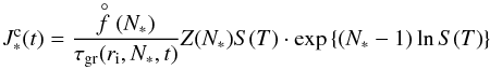 (1)with N∗ the critical cluster size (see Eq. (12)). The equilibrium cluster size distribution,
  [cm-3], can be considered a Boltzmann-like distribution in local thermal equilibrium,
 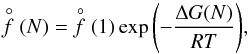 (2)where
  (1) [cm-3] is the equilibrium number density of the monomer (smallest cluster unit like TiO2 or SiO) and ΔG(N) [kJ mol-1] the Gibbs free energy change due to the formation of a cluster of size N from the saturated vapour at temperature T. The rate of growth for each individual cluster of size N is
  (3)where
  [cm2] is the reaction surface area of an N-sized cluster, N is the number of monomers in a cluster, a0 the hypothetical monomer radius, α is the efficiency of the reaction (assumed to be 1), vrel [cm2s-1] is the relative velocity between a monomer and the cluster and nf [cm-3] the particle density of the molecule for the growth (forward) reaction (≡(1)). The relative velocity is approximated by the thermal velocity (see Eq. (15) in Helling et al. 2001)
 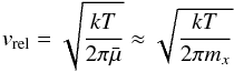 (4)with
  , where mx is the mass of the monomer molecule (e.g. TiO2) and mV the mass of a grain with volume V. For macroscopic grains, mV ≫ mx, hence
  . Equation (1) also contains the supersaturation ratio SN of a cluster with N monomers
  with the saturation vapour pressure
  (5)ΔG(N) can be expressed by a relationship to the standard molar Gibbs free energies in reference state “°−” (measured at a standard gas pressure and gas temperature) of formation for cluster size N
 (6)Combining Eqs. (5) and (6) results in
  (7)where the right-hand side contains standard state values only (
 (N) – standard Gibbs free energy of formation of cluster size N, (1) – standard Gibbs free energy of the monomer,
  (s) – standard Gibbs free energy of formation of the solid phase) which can be found by experiment or computational chemistry. We use the JANAF thermochemical table (Chase et al. 1985) where the standard states are given at
  K and
K and  bar.
bar.
The classical nucleation theory assumes that the detailed knowledge about ΔG(N) can be encapsulated by the value of the surface tension, σ∞, of the macroscopic solid such that  (8)The dependence of the surface energy on cluster size is therefore neglected. The Zeldovich factor (contribution from Brownian motion to nucleation rate) in Eq. (1) is
  (9)The nucleation rate can now be expressed as
 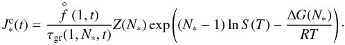 (10)
(10)
2.1.2. Modified classical nucleation theory
A modified nucleation theory was proposed by Draine et al. (1977) and Gail et al. (1984) by taking into account the curvature on the surface energy for small clusters (Gail et al. 1984). Equation (8) changes to 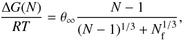 (11)where Nf is a fitting factor representing the particle size at which the surface energy is reduced to half of the bulk value. This fitting factor allows a critical cluster N∗ to be calculated as
 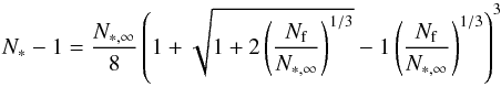 (12)with
 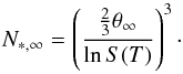 (13)
(13)
2.1.3. Non-classical nucleation theory
If cluster data are available, J∗ can be calculated using cluster number densities, growth rates and evaporation rates of each cluster size as J∗ is a flux through cluster space, 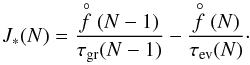 (14)Applying the Becker-Döring method (see Gail & Sedlmayr 2014), f(2) can be eliminated from the N = 2 equation using the N = 3 equation, then again for f(3) and so on, resulting in the summation
 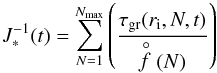 (15)with Eq. (3) for τgr. The number density of a cluster of size N is
 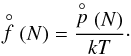 (16)The partial pressures can be calculated from the law of mass action applied to an N-cluster,
 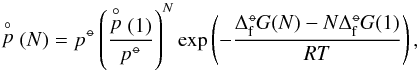 (17)with
  (1) [dyn cm-2] the partial pressure of the monomer number density; (1) will be calculated as local thermodynamic equilibrium (LTE) allowing the application of our equilibrium chemistry routine (Sect. 3.1.2).
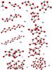 |
Fig. 1 Geometry of the calculated (TiO2)N structures. Molecules labelled “a” are the molecules calculated by Jeong et al. (2000) and those labelled “b” or unlabelled are the current most stable cluster geometries (Calatayud et al. 2008; Syzgantseva et al. 2011). Grey balls represent Ti atoms while red represent O atoms. |
2.2. Approach
2.2.1. Computational aspects
All cluster calculations were performed using the B3LYP (Lee et al. 1988) density functional theory with basis set 6-311G(d) as part of the Gaussian (Frisch et al. 2009) computational chemistry package. This level of theory was used for its mix of accuracy and computational speed and to keep in line the previous investigations on the same molecules (Jeong et al. 2000; Calatayud et al. 2008; Syzgantseva et al. 2011). B3LYP is a popular and well regarded density functional theory for metal oxides and other inorganic compounds. The reference state of the clusters was at temperature T°− = 298.15 K and pressure p°− = 1 bar. These were chosen so that the JANAF thermochemical tables for the elemental thermochemical values could be used to calculate the Gibbs free energies of the molecules. Gaussian calculates the partition function of a molecule using thermodynamical laws with contributions from the rotational, translational, vibrational and electronic motions of the molecule. Therefore, it can generate enthalpies (Δ H) and Gibbs energies (Δ G) for any molecule to a good degree of accuracy depending only on the functional and basis set used. These enthalpies and Gibbs free energies can then be used to find the formation energies of the molecules with basic thermodynamics (Sect. 2.3). Previous studies of these TiO2 cluster geometries (Calatayud et al. 2008; Syzgantseva et al. 2011) have focused on the reactivity and electronic structure of the clusters and not specifically on the thermodynamics of the formation of the clusters themselves.
2.2.2. Cluster geometries
The main difference between past investigations and the current study are the calculation of updated TiO2 cluster geometries. Figure 1 summarises both the original geometries from Jeong et al. (2000) labelled “a”, with the new results labelled “b” or unlabelled. These geometries can mostly be found in the chemistry literature (Calatayud et al. 2008; Syzgantseva et al. 2011; Richard et al. 2010) except for a new stable N = 7.
The linear, polymer-like (TiO2)N chains investigated in Jeong et al. (2000) are less stable than their more compressed counterparts published by Calatayud et al. (2008) and Syzgantseva et al. (2011). This is shown by the higher binding energies for the compressed structures (Appendix A). These binding energies have a direct impact on the Gibbs formation energies of the clusters and there will be significant differences between the two geometries. Furthermore, it is assumed that over time the molecules will configure to their lowest energy state geometry and so other less stable configurations are not considered further.
2.3. Results for thermodynamic quantities for TiO2 clusters
Applying the results of the computation to thermodynamical identities allows the calculation of the Gibbs free energies of the clusters. The Gibbs energy of formation can be calculated from 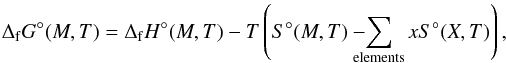 (18)where M is the molecular/cluster values and X the constituent atoms. In order to find the enthalpy of formation of a cluster at temperature T the enthalpy of formation at 0 K must first be calculated. This is given by
 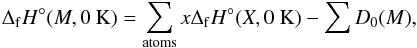 (19)where x is the total number of elements X in the molecule and D0(M) the reduced atomization energy of the molecule. The ΔfH°(X,0K) of Ti and O can be found in the JANAF thermochemical tables. The reduced atomization energy is defined as
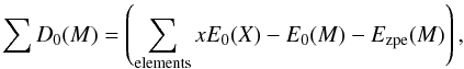 (20)where E0(X) and E0(M) are the internal energy of the elements and the molecule and Ezpe(M) the zero-point energy of the molecule. All the total energy terms (E0(X), E0(M), and Ezpe(M)) can be calculated from the Gaussian 09 output. The crucial quantity of the elemental atomization energies(E0(X)) of both Ti and O was computed using the same level of theory (B3LYP 6-311G(d)) as the clusters.
When the enthalpy of formation at 0 K is calculated for each cluster, we can find the enthalpy of formation at a reference temperature (T°− = 298.15 K) as 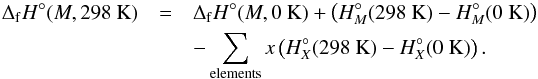 (21)The enthalpy of formation at arbitrary temperature T can then be found by a similar calculation:
 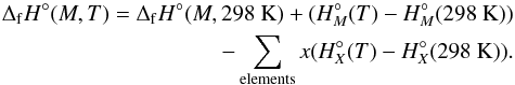 (22)The entropy of the clusters are calculated from the relation S = (H − G) /T where H and G are the enthalpy and Gibbs energies, respectively. The entropy of the constituent elements at various temperatures are from the JANAF thermochemical tables.
Calculated thermochemical tables and Gibbs free energies for the (TiO2)N clusters are provided in Appendix B.
 |
Fig. 2 TiO2ΔfG(N) /N with respect to N for T = 1000 K. The blue triangles represent the new geometry isomers while red represent the molecules found in Jeong et al. (2003). The red line is the modified expression with σ∞ = 618 erg cm-2 and the black with σ∞ = 490 erg cm-2. |
2.3.1. Surface tension of TiO2
Surface tension is a measure of surface energy density of the bulk property of a solid. We approximate the bulk surface tension, σ∞, by fitting the small clusters to the modified nucleation theory using the calculated Gibbs free energies. Combining Eqs. (6) and (11), the Gibbs formation energy of cluster size N is 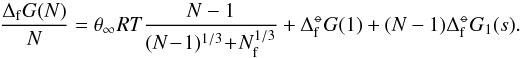 (23)By plotting ΔGf(N) /N against N for the clusters, a best fit σ∞ can be found for different temperatures. Figure 2 shows this fitting process for T = 1000 K. The original surface tension value from Jeong et al. (2000), σ∞ = 618 erg cm-2, is also shown for comparison. The values for
  are from the JANAF tables and Nf = 0 is used for all calculations. The new cluster geometries have a lower Gibbs energy of formation than the old clusters as a consequence of their increased stability. By fitting σ∞ we show that there is a slight temperature dependence (Fig. 3) on the best fit value. In the range Tgas = 500 − 2000 K the surface tension can be approximated by the linear relationship
  (24)The mean value over this temperature range yields an approximate surface tension of σ∞ = 480.6 erg cm-2.
3. The abundances of molecules and clusters in the gas phase
The seed formation rates depend on the gas-phase composition and the abundance of the monomer gas-species in comparison. We therefore summarise the abundances of the Ti-binding gas-species and we include Si-binding molecules for later considerations of SiO nucleation based on updated SiO vapour pressure data. We apply our thermodynamic cluster data to explore the abundance of the TiO2 clusters shown in Fig. 1 and their relative changes.
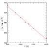 |
Fig. 3 Temperature dependence of best fit σ∞ for the range Tgas = 500 − 2000 K. Triangles denote best fit values to the modified nucleation expression. |
3.1. Approach
We utilize one example model atmosphere structure (Teff = 1600 K, log(g) = 3.0, solar metallicity) from the Drift-Phoenix atmosphere grid that is representative for the atmosphere of a giant gas planet and for brown dwarfs. This combination of global parameters also includes the atmosphere of the group of recently discovered low-gravity brown dwarfs (Faherty et al. 2013). We use the model (Tgas, pgas) structure as input for our external chemical equilibrium program to calculate the chemical gas composition in more detail than necessary for the Drift-Phoenix models.
3.1.1. Drift-Phoenix model atmosphere
Drift-Phoenix (Dehn 2007; Helling et al. 2008b; Witte et al. 2009) model atmosphere simulations solve the classical 1D model atmosphere problem coupled to a kinetic phase-non-equilibrium cloud formation model. Each of the model atmospheres is determined by the effective temperature (Teff [K]), the surface gravity (log(g), with g in cm/s2) and element abundances. The cloud’s opacity is calculated applying Mie and effective medium theory.
In addition to details of the dust clouds like height-dependent grain sizes and the height-dependent composition of the mixed-material cloud particles, the atmosphere model provides us with atmospheric properties such as the local convective velocity, the temperature-pressure (Tgas [K], pgas [dyn/cm2]) structure and the dust-depleted element abundances. The local temperature is the result of the radiative transfer solution, the local gas pressure of the hydrostatic equilibrium and the element abundances are the result of the element conservation equations that include the change of elements by dust formation and evaporation.
3.1.2. Chemical equilibrium routine
A combination of 155 gas-phase molecules (including 33 complex carbon-bearing molecules), 16 atoms and various ionic species were used under the assumption of LTE. For more details, please refer to Bilger et al. (2013) and Helling et al. (2000) for the thermodynamical data used. The Grevesse et al. (2007) solar composition is used to calculate the gas-phase chemistry outside the metal depleted cloud layers and before cloud formation. No solid particles were included in the chemical equilibrium calculations. However, their presence influences the gas phase by reducing element abundances from cloud formation and the impact of the cloud opacity on the radiation field, both accounted for in the Drift-phoenix model simulations. We utilize Drift-Phoenix model atmosphere (Tgas, pgas) structures as input for our calculations.
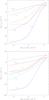 |
Fig. 4 Comparison of number densities (cm-3) for different Ti-binding (top) and Si-binding (bottom) molecules for a Drift-Phoenix (Tgas, pgas) structure for Teff = 1600 K, log(g) = 3.0 and solar metallicity. |
3.2. Results for molecule and cluster abundances
As pressure and temperature increase in the atmosphere, the abundance of all gas species increase in chemical equilibrium (Fig. 4). For comparison, both Ti and Si combinations are shown because the number densities of TiO2 and SiO are input properties for Eqs. (10) and (17). The SiO molecule generally has a higher number density than TiO2 since the element abundance of Si is considerably larger than that of Ti. This might suggest that SiO is a more suitable nucleation species than TiO2 and we will investigate this question in Sects. 4.2 and 5. Figure 4 (top) demonstrates that TiO2 is the most abundant Ti-binding gas species in almost the entire atmosphere followed by TiO and the Ti atom. The molecule TiO is more abundant than TiO2 in the high-temperature part of the atmospheric structure; SiO is the most abundant Si-binding molecules followed by SiO2 and Si.
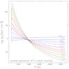 |
Fig. 5 Partial pressures |
As part of our assessment of the TiO2 nucleation, we show the partial pressure,  [dyn cm-2] (Eq. (17)), for each (TiO2)N cluster in Fig. 5. Both (1) (=nTiO2kTgas) and (2) maintain fairly constant pressures. For N> 2, the curves become more dynamic. They start at higher and higher magnitudes, increase quickly, and then drop off. The order of the curves is also interesting, with the higher N partial pressures reaching higher values at lower temperature (lower gas pressures). These findings support our expectation that bigger clusters become more stable and more abundant with decreasing temperatures and that they are unstable and of low abundance at high temperatures.
4. Seed formation rates
Based on the results from Sects. 2.3.1 and 2.3.2, we are now in the position to calculate and compare seed formation rates (nucleation rates). We present our updated results for TiO2 as the nucleation species considered in our previous works. We compare SiO nucleation based on updated vapour pressure data. Gail et al. (2013) has recently suggested that SiO nucleation could be more efficient than TiO2 nucleation. We will test this hypothesis here and as part of our cloud formation model in Sect. 5.
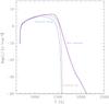 |
Fig. 6 Nucleation rates J∗ with three methods: classical with σ∞ = 618 erg cm-2, Jeong et al. (2000); classical with temperature dependent σ∞; and non-classical based on Gibbs free energies for TiO2. |
4.1. TiO2 nucleation rate
Results for classical nucleation theory:
Surface tension values have a direct impact on the nucleation rate in the classical nucleation theory approach (Sect. 2.1.1). In order to assess this impact, the new TiO2 surface tension was tested in our nucleation routines and nucleation rates calculated for a given (Tgas, pgas) model atmosphere profile. Figure 6 demonstrates that the difference in nucleation rate, J∗, from our new data to the value from Jeong et al. (2000) is not very significant.
Results for non-classical nucleation theory:
Converting all partial pressures, , for all (TiO2)N cluster into number densities allows us to use the Becker-Döring method to calculate the nucleation rate J∗ (Gail & Seldmayr 2014). This is different from the classical nucleation rate in that we use the Gibbs free energies of formation for each individual cluster without the need to derive a surface tension.
Figure 6 shows that at the lowest temperatures, the non-classical nucleation rate increases quickly with the temperature until 700 K where the rate increases more slowly to around 1800 K, and then drops (though not as quickly as the classical curves). At the higher temperatures, the molecules will have sufficient energy so that when they collide they will break apart just as often as they coalesce. Though the non-classical values are visibly different from the classical, they are similar in magnitude to the classical data with a temperature varying σ∞, particularly in the 700−1500 K region of the model atmosphere considered here.
4.2. SiO nucleation
Stimulated by the recent paper by Gail et al. (2013), we compare the nucleation rate of SiO to our TiO2 values from the previous sections. Since the number density of SiO is much greater than TiO2, it is reasonable to expect that the nucleation rate for SiO would also be larger than that of TiO2. Gail et al. (2013) provide the following analytic expression for the SiO nucleation rate including the updated vapour pressure from Wetzel et al. (2013), (25)where
  (1) and all other variables have the same meaning as before. Calculating
  for the same model atmosphere structure as before, we find that SiO nucleates at a much higher rate compared to our TiO2 results. We also demonstrate in Fig. 7 the changes in the SiO nucleation rates alone through the update in vapour pressure data, J∗ ,Paguette vs. J∗ ,Gail. There are similarities between the two SiO rates, the double peaks occur at approximately the same temperatures, indicating that both methods create similar effects at these temperatures. These differences resulting from updated vapour pressure data cannot account for the differences between the SiO and the TiO2 nucleation rates.
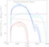 |
Fig. 7 Number densities (cm-3) and nucleation rates J∗ (s-1cm-3) for both TiO2 and SiO. Number densities calculated from the Drift-Phoenix model (Helling et al. 2006). J∗ ,Jeong is the classical nucleation rate calculated with σ∞ = 618 erg cm2; J∗ ,Lee is calculated with temperature dependent σ∞. J∗ ,Paquette and J∗ ,Gail have both been calculated using new vapour pressures (Wetzel et al. 2013). Blue lines surrounding J∗ ,Gail are the upper and lower boundaries. These nucleation rates were calculated for an undepleted gas-phase. |
5. Impact on cloud formation
Cloud formation in brown dwarfs and giant gas planets needs to start with the formation of condensation seeds in contrast to the Earth where weather cloud formation is started through the injection of seed particles (e.g. volcano eruptions or sand storms) into the atmosphere. Jeong et al. (1999) demonstrate that it is not obvious which species would be the best choice for a nucleation species as part of a dust/cloud particle formation model. Gail et al. (2013) and Helling & Fomins (2013) further argue that the complex silicate seeds (e.g. Mg2SiO4[s], Al2O3[s]) can only form from molecules that are available in the gas-phase. The SiO and TiO2 are available in abundance in the gas phase (Fig. 4), but Mg2SiO4 does not exist as a molecule, and Al2O3 is extremely rare (e.g. Fig. 5 in Helling & Woitke 2006). Other Mg or Al binding molecules are abundant pointing to the possibility of heterogeneous nucleation. Hence, the formation of seed particles does not need to proceed via a homomolecular homogeneous nucleation, but may well be formed by heteromolecular homogeneous nucleation (e.g. Goumans & Bromley 2013; Plane 2013). Because of the lack of cluster data for more complex nucleation paths, we consider homomolecular homogeneous nucleation only.
In principle, the condensing material does not care which seed particle is available as long as there is a surface to condense on. The need to identify the first condensate or the most efficient nucleation species arises if a model is built in order to study dust forming systems, for example, clouds in brown dwarfs and exoplanets, or dust in circumstellar shells. The two best candidates with respect to stability and abundance in the gas phase are TiO2 and SiO. We are now in the position to test how the new material data for TiO2 (Sect. 2.3) and the updated saturation vapour pressure for SiO (Eq. (25)) affect our cloud formation results. Our results in this paper have so far lead us to expect only moderate differences from the updated TiO2 nucleation rate (Fig. 6), but substantial differences if considering SiO instead of TiO2 as the nucleation species. Figure 7 suggests a considerably more efficient SiO seed formation compared to TiO2 seed formation. In this section, we will demonstrate that it is misleading to consider seed formation as a single process. The nucleation process needs to be considered in combination with other element consuming cloud/dust formation processes in order to reliably approach the question about the most suitable condensation seed species.
5.1. Approach
We assess the impact of the nucleation description that is part of our cloud formation model on the resulting cloud structure details. Our cloud formation model describes the formation of clouds by nucleation, subsequent growth by chemical surface reactions on-top of the seeds, evaporation, gravitational settling, element conservation, and convective replenishment (Woitke & Helling 2003, 2004; Helling & Woitke 2006; Helling et al. 2008a). The effect of nucleation, growth, and evaporation on the remaining elements in the gas phase is fully accounted for (Eqs. (10) in Helling et al. 2008a). The surface growth causes the grains to grow to μm-sized particles of a mixed composition of those solids taken into account. For this study, we consider 12 growth species that grow by 60 gas-solid surface reactions (Helling et al. 2008a). We use the same Drift-Phoenix model atmosphere as described in Sect. 3.1 as input for our more complex cloud formation code.
5.2. Results
Figure 8 demonstrates the impact of the nucleation treatment on the cloud formation processes and the resulting cloud properties. Most importantly, if considered as part of an interacting set of processes, the TiO2 seed formation is more efficient than the SiO seed formation (top panel with nucleation rates) which deviates from our previous expectation triggered by Fig. 7. The reason is that the elements Si and O are part of many silicate materials (SiO2[s], MgSiO3[s], Mg2SiO4[s], etc.) that are already thermally stable and therefore grow efficiently as soon as the seed particles emerge from the gas phase. Ti-binding growth species are much less abundant because of the low Ti element abundances to start with (Fig. 4). Hence, an assessment of the importance of a seed forming species always needs to be performed in connection with the growth process, else it leads to wrong conclusions regarding the best suited nucleation species. As a consequence of SiO being a very inefficient nucleation species, fewer cloud particles form. Figure 8 (middle) shows that a SiO-seeded cloud would have >103 times fewer cloud particles with an increasing difference for increasing atmospheric depth. Instead, the material is consumed by growth leading to grains up to a size of 100 μm at the inner cloud edge.
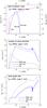 |
Fig. 8 TiO2 and SiO nucleation rates (top) calculated as part of the cloud formation model and their effect on the number density of cloud particles (middle) and the mean grain size (bottom). The calculations include nucleation, growth/evaporation, element conservation, gravitational settling, and convective replenishment. The same Drift-Phoenix model structure for Teff = 1600 K, log (g) = 3.0, and solar metallicity as in Fig. 6 was used. |
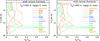 |
Fig. 9 Differences in the cloud particle material compositions for TiO2 nucleation (left) and SiO (right). The nucleation species (TiO2 or SiO molecule) are also surface growth species (as in Table 1 in Helling et al. 2008a). The main differences occur in the uppermost part of the cloud, the haze layer: SiO[s]/MgO[s] with impurities of FeS[s], FeO[s], Fe2O3[s], and Al2O3[s] in the case of SiO nucleation (right), and MgSiO3[s]/Mg2SiO4[s] with impurities of all other solids plus a very thin TiO2[s] layer at the very top in the case of TiO2[s] nucleation (left). |
Figure 9 demonstrates that the overall mean material composition of the mineral cloud does not change significantly between TiO2-seeded and SiO-seeded clouds. However, the uppermost part, which is often referred to as the haze layer, has a fundamentally different composition depending on the condensation seed species considered: SiO[s]/MgO[s] with impurities of FeS[s], FeO[s], Fe2O3[s], and Al2O3[s] in the case of SiO nucleation, and MgSiO3[s]/Mg2SiO4[s] with impurities of all other solids plus a very thin TiO2[s] layer at the very top in the case of TiO2[s] nucleation.
6. Summary
The formation of condensation seeds is the initial step to cloud formation in astrophysical objects without a crust, for example supernovae, AGB-stars, M-dwarfs, brown dwarfs, and giant gas planets. The long-standing question is whether it is possible to identify a first condensate that kicks off the whole condensation process. This question has long been debated. High-temperature condensates such as solid iron seeds forming from (Fe)N gas phase clusters (John & Sedlmayr 1997) or MgO seeds forming from (MgO)N clusters (Köhler & Sedlmayr 1997) were dismissed because large clusters were thermodynamically unstable or they were not very abundant. Instead, TiO2 seed formation is attractive because of the stability of the (TiO2)N clusters and their relative abundance. The same arguments are made for SiO, but despite SiO’s higher abundance compared to TiO2, its nucleation rate did fall short of TiO2 (Jeong et al. 2000). Gail et al. (2013) reconsider SiO nucleation for AGB stars and suggest that it might be a favourable seed formation species based on new vapour data. Based on updated (TiO2)N clusters we investigate under which conditions this finding could be relevant for substellar atmospheres.
In this paper, we have presented updated Gibbs free energies of TiO2 clusters using computational chemistry for newly available molecule geometries (Calatayud et al. 2008; Syzgantseva et al. 2011). The more stable cluster geometries compared to Jeong et al. (2000) from chemistry literature yielded a temperature dependent surface tension with an average value of σ∞ = 480.6 erg cm-2 when fitted with the modified nucleation theory model. This new surface tension was then used in conjunction with chemical abundance routines to calculate a nucleation rate for various temperatures and TiO2 number densities for an example atmosphere representative of a young brown dwarf or a giant gas planet. The new value approximately doubles the rate of nucleation for the species. The non-classical TiO2 nucleation rate was calculated using the newly calculated Gibbs free energies which obtained higher results than those obtained through classical means. Inspired by newly available vapour pressure data, we show that SiO nucleation can only be more efficient than TiO2 nucleation if no other element depletion processes are taking place. Hence, TiO2 remains the more efficient nucleation species of the two because nucleation and surface growth will take place simultaneously and because both processes require a supersaturated gas.
Online material
Appendix A: Energy tables
In the following tables “Jeong’s Geometry” or similar refers to the original geometries found in Jeong et al. (2000) and “Bromley’s Geometry” or similar refers to the current (2012) most stable (TiO2)N cluster geometries.
DFT/B3LYP energies for Ti, O, and (TiO2)n.
Binding energies for (TiO2)n clusters.
Chemical information on the atoms Ti and O.
Appendix B: Thermochemical Tables of (TiO2)N
Calculated thermochemical values of TiO2.
Calculated thermochemical values of (TiO2)2.
Calculated thermochemical values of Jeong’s (TiO2)3.
Calculated thermochemical values of Bromley’s (TiO2)3.
Calculated thermochemical values of Jeong’s (TiO2)4.
Calculated thermochemical values of Bromley’s (TiO2)4.
Calculated thermochemical values of Jeong’s (TiO2)5.
Calculated thermochemical values of Bromley’s (TiO2)5.
Calculated thermochemical values of Jeong’s (TiO2)6.
Calculated thermochemical values of Bromley’s (TiO2)6.
Calculated thermochemical values of Bromley’s (TiO2)7.
Calculated thermochemical values of Bromley’s (TiO2)8.
Calculated thermochemical values of Bromley’s (TiO2)9.
Calculated thermochemical values of Bromley’s (TiO2)10.
Acknowledgments
We highlight financial support of the European Community under the FP7 by an ERC starting grant. We are very grateful for a scholarship fund for E.L. and H.G. by the Royal Astronomical Society. We thank Peter Woitke for general discussions on the paper’s topic. The computer support at the School of Physics & Astronomy in St Andrews is gratefully acknowledged.
References
- Bilger, C., Rimmer, P. B., & Helling, C. 2013, MNRAS, 435, 1888 [NASA ADS] [CrossRef] [Google Scholar]
- Bromley, S. T., Moreira, I. P. R., Neyman, K. M., & Illas, F. 2009, Chem. Soc. Rev, 38, 2657 [CrossRef] [Google Scholar]
- Calatayud, M., Maldonado, L., & Minot, C. 2008, J. Phys. Chem. C, 112, 16087 [CrossRef] [Google Scholar]
- Catlow, C. R. A., Bromley, S. T., Hamad, S., et al. 2010, Phys. Chem. Chem. Phys., 12, 786 [NASA ADS] [CrossRef] [Google Scholar]
- Chase, M. W., Davies, C. A., Downey, J. R., et al. 1985, NIST-JANAF thermochemical tables, 3rd edn., J. Phys. Chem. Ref. Data, 14 [Google Scholar]
- Copperwheat, C. M., Wheatley, P. J., Southworth, J., et al. 2013, MNRAS, 434, 661 [NASA ADS] [CrossRef] [Google Scholar]
- Demyk, K., Heijnsbergen, D., Helden, G., & Meijer, G. 2004, A&A, 420, 547 [NASA ADS] [CrossRef] [EDP Sciences] [Google Scholar]
- Dehn, M. 2007, Ph.D. Thesis, Univ. Hamburg, Germany [Google Scholar]
- Faherty, J., Rice, E., Cruz, K. L., Mamajek, E. E., & Nunez, A. 2013, AJ, 145, 2 [CrossRef] [Google Scholar]
- Frisch, M. J., Trucks, G. W., Schlegel, H. B., et al. 2009, Gaussian 09 Revision D.01, Gaussian Inc. Wallingford CT [Google Scholar]
- Gail, H. P., & Sedlmayr, E. 1986, A&A, 166, 225 [NASA ADS] [Google Scholar]
- Gail, H. P., & Sedlmayr, E. 2014, Physics and Chemistry of Circumstellar Dust Shells (Cambridge University Press), 52 [Google Scholar]
- Gail, H. P., Keller, R., & Sedlmayr, E. 1984, A&A, 133, 320 [Google Scholar]
- Gail, H. P., Wetzel, S., Pucci, A., & Tamanai, A. 2013, A&A, 555, A119 [NASA ADS] [CrossRef] [EDP Sciences] [Google Scholar]
- Grevesse, N., Asplund, M., & Sauval, A. J. 2007, Space Sci. Rev., 130, 105 [Google Scholar]
- Goumans, T. P. M., & Bromley, S. T. 2013, Phil. Trans. R. Soc. A, 371, 0580 [Google Scholar]
- Helling, Ch. 2007, Proc. IAU, 2, 224 [Google Scholar]
- Helling, Ch., & Fomins, A. 2013, Phil. Trans. R. Soc. A, 371 [Google Scholar]
- Helling, Ch., & Woitke, P. 2006, A&A, 455, 325 [NASA ADS] [CrossRef] [EDP Sciences] [Google Scholar]
- Helling, Ch., Winters, J.-M., & Sedlmayr, E. 2000, A&A, 358, 651 [NASA ADS] [Google Scholar]
- Helling, Ch., Oevermann, M., Lüttke, M. J. H., Klein, R., & Sedlmayr, E. 2001, A&A, 376, 194 [NASA ADS] [CrossRef] [EDP Sciences] [Google Scholar]
- Helling, Ch., Woitke, P., & Thi, W.-F. 2008a, A&A, 485, 547 [NASA ADS] [CrossRef] [EDP Sciences] [Google Scholar]
- Helling, Ch., Dehn, M., Woitke, P., & Hauschildt, P. H. 2008b, ApJ, 675, L105 [NASA ADS] [CrossRef] [Google Scholar]
- Helling, Ch., Ackerman, A., Allard, F., et al. 2008c, MNRAS, 391, 1854 [NASA ADS] [CrossRef] [Google Scholar]
- Jeong, K. S., Winters, J. M., & Sedlmayr, E. 1999, Asymptotic Giant Branch Stars, IAU Symp., 191, 233 [Google Scholar]
- Jeong, K. S., Chang, C., Sedlmayr, E., & Sülzle, D. 2000, J. Phys. B, 33, 3417 [NASA ADS] [CrossRef] [Google Scholar]
- Jeong, K. S, Winters, J. M., Le Bertre, T., & Sedlmayr, E. 2003, A&A, 407, 191 [NASA ADS] [CrossRef] [EDP Sciences] [Google Scholar]
- John, M., & Sedlmayr, E. 1997, ApSS, 251, 219 [NASA ADS] [Google Scholar]
- Köhler, T. M., & Sedlmayr, E. 1997, A&A, 310, 553 [Google Scholar]
- Lecavelier Des Etangs, A., Pont, F., Vidal-Madjar, A., & Sing, D. 2008, A&A, 481, 83 [Google Scholar]
- Lee, C., Yang, W., & Parr, R. G. 1988, Phys. Rev. B, 37, 785 [Google Scholar]
- Miller-Ricci Kempton, E., Zahnle, K., & Fortney, J. J. 2012, ApJ, 745, 3 [NASA ADS] [CrossRef] [Google Scholar]
- Patzer, A. B. C., Gauger, A., & Sedlmayr, E. 1998, A&A, 337, 847 [Google Scholar]
- Plane, J. M. C. 2013, Phil. Trans. R. Soc. A, 371, 0335 [Google Scholar]
- Pont, F., Sing, D. K., Gibson, N. P., et al. 2013, MNRAS, 432, 2917 [NASA ADS] [CrossRef] [Google Scholar]
- Schlawin, E., Zhao, M., Teske, J. K., & Herter, T. 2014, ApJ, 783, 5 [NASA ADS] [CrossRef] [Google Scholar]
- Sing, D. K., Pont, F., Aigrain, S., et al. 2011, MNRAS, 416, 1443 [NASA ADS] [CrossRef] [Google Scholar]
- Sing, D. K., Lecavelier des Etangs, A., Fortney, J. J., et al. 2013, MNRAS, 436, 2956 [NASA ADS] [CrossRef] [Google Scholar]
- Syzgantseva, O. A, Gonzalez-Navarrete, P., Calatayud, M., Bromley, S. T., & Minot, C. 2011, J. Phys. Chem. C, 115, 15890 [CrossRef] [Google Scholar]
- Wetzel, S., Klevenz, M., Gail, H.-P., Pucci, A., & Trieloff, M. 2013, A&A, 553, A92 [NASA ADS] [CrossRef] [EDP Sciences] [Google Scholar]
- Witte, S., Helling, Ch., & Hauschildt, P. 2009, A&A, 506, 1367 [NASA ADS] [CrossRef] [EDP Sciences] [Google Scholar]
- Woitke, P., & Helling, C. 2003, A&A, 399, 297 [NASA ADS] [CrossRef] [EDP Sciences] [Google Scholar]
- Woitke, P., & Helling, C. 2004, A&A, 414, 335 [NASA ADS] [CrossRef] [EDP Sciences] [Google Scholar]
All Tables
All Figures
|
Fig. 1 Geometry of the calculated (TiO2)N structures. Molecules labelled “a” are the molecules calculated by Jeong et al. (2000) and those labelled “b” or unlabelled are the current most stable cluster geometries (Calatayud et al. 2008; Syzgantseva et al. 2011). Grey balls represent Ti atoms while red represent O atoms. |
| In the text | |
|
Fig. 2 TiO2ΔfG(N) /N with respect to N for T = 1000 K. The blue triangles represent the new geometry isomers while red represent the molecules found in Jeong et al. (2003). The red line is the modified expression with σ∞ = 618 erg cm-2 and the black with σ∞ = 490 erg cm-2. |
| In the text | |
|
Fig. 3 Temperature dependence of best fit σ∞ for the range Tgas = 500 − 2000 K. Triangles denote best fit values to the modified nucleation expression. |
| In the text | |
|
Fig. 4 Comparison of number densities (cm-3) for different Ti-binding (top) and Si-binding (bottom) molecules for a Drift-Phoenix (Tgas, pgas) structure for Teff = 1600 K, log(g) = 3.0 and solar metallicity. |
| In the text | |
|
Fig. 5 Partial pressures |
| In the text | |
|
Fig. 6 Nucleation rates J∗ with three methods: classical with σ∞ = 618 erg cm-2, Jeong et al. (2000); classical with temperature dependent σ∞; and non-classical based on Gibbs free energies for TiO2. |
| In the text | |
|
Fig. 7 Number densities (cm-3) and nucleation rates J∗ (s-1cm-3) for both TiO2 and SiO. Number densities calculated from the Drift-Phoenix model (Helling et al. 2006). J∗ ,Jeong is the classical nucleation rate calculated with σ∞ = 618 erg cm2; J∗ ,Lee is calculated with temperature dependent σ∞. J∗ ,Paquette and J∗ ,Gail have both been calculated using new vapour pressures (Wetzel et al. 2013). Blue lines surrounding J∗ ,Gail are the upper and lower boundaries. These nucleation rates were calculated for an undepleted gas-phase. |
| In the text | |
|
Fig. 8 TiO2 and SiO nucleation rates (top) calculated as part of the cloud formation model and their effect on the number density of cloud particles (middle) and the mean grain size (bottom). The calculations include nucleation, growth/evaporation, element conservation, gravitational settling, and convective replenishment. The same Drift-Phoenix model structure for Teff = 1600 K, log (g) = 3.0, and solar metallicity as in Fig. 6 was used. |
| In the text | |
|
Fig. 9 Differences in the cloud particle material compositions for TiO2 nucleation (left) and SiO (right). The nucleation species (TiO2 or SiO molecule) are also surface growth species (as in Table 1 in Helling et al. 2008a). The main differences occur in the uppermost part of the cloud, the haze layer: SiO[s]/MgO[s] with impurities of FeS[s], FeO[s], Fe2O3[s], and Al2O3[s] in the case of SiO nucleation (right), and MgSiO3[s]/Mg2SiO4[s] with impurities of all other solids plus a very thin TiO2[s] layer at the very top in the case of TiO2[s] nucleation (left). |
| In the text | |
Current usage metrics show cumulative count of Article Views (full-text article views including HTML views, PDF and ePub downloads, according to the available data) and Abstracts Views on Vision4Press platform.
Data correspond to usage on the plateform after 2015. The current usage metrics is available 48-96 hours after online publication and is updated daily on week days.
Initial download of the metrics may take a while.