| Issue |
A&A
Volume 685, May 2024
|
|
|---|---|---|
| Article Number | A106 | |
| Number of page(s) | 26 | |
| Section | Catalogs and data | |
| DOI | https://doi.org/10.1051/0004-6361/202348264 | |
| Published online | 15 May 2024 | |
The SRG/eROSITA All-Sky Survey
The first catalog of galaxy clusters and groups in the Western Galactic Hemisphere★
1
Max Planck Institute for Extraterrestrial Physics,
Giessenbachstrasse 1,
85748
Garching,
Germany
e-mail: ebulbul@mpe.mpg.de
2
Hamburg Observatory, University of Hamburg,
Gojenbergsweg 112,
21029
Hamburg,
Germany
3
IRAP, Université de Toulouse, CNRS, UPS, CNES,
31028
Toulouse,
France
4
Universitäts-Sternwarte, LMU Munich,
Scheinerstr. 1,
81679
München,
Germany
5
Universität Innsbruck, Institut für Astro- und Teilchenphysik,
Technikerstr. 25/8,
6020
Innsbruck,
Austria
6
Arnold Sommerfeld Center for Theoretical Physics, LMU Munich,
Theresienstr. 37,
80333
München,
Germany
7
Leibniz-Institut für Astrophysik Potsdam (AIP),
An der Sternwarte 16,
14482
Potsdam,
Germany
8
Argelander-Institut für Astronomie (AIfA), Universität Bonn,
Auf dem Hügel 71,
53121
Bonn,
Germany
Received:
13
October
2023
Accepted:
2
January
2024
Clusters of galaxies can be used as powerful probes to study astrophysical processes on large scales, test theories of the growth of structure, and constrain cosmological models. The driving science goal of the SRG/eROSITA All-Sky Survey is to assemble a large sample of X-ray clusters with a well-defined selection function to determine the evolution of the mass function and, hence, the cosmological parameters. We present here a catalog of 12 247 optically confirmed galaxy groups and clusters detected in the 0.2–2.3 keV as extended X-ray sources in a 13 116 deg2 region in the western Galactic half of the sky, which eROSITA surveyed in its first six months of operation. The clusters in the sample span the redshift range 0.003 < z < 1.32. The majority (68%) of these clusters, 8361 sources, represent new discoveries without known counterparts in the literature. The mass range of the sample covers three orders of magnitude from 5 × 10¹² Msun to 2 × 10¹⁵Msun. We construct a sample for cosmology with a higher purity level (~95%) than the primary sample, comprising 5259 securely detected and confirmed clusters in the 12791 deg2 common footprint of eRASS1 and the DESI Legacy Survey DR10. We characterize the X-ray properties of each cluster, including their flux, luminosity and temperature, the total mass, gas mass, gas mass fraction, and mass proxy YX. These are determined within two apertures, 300 kpc, and the overdensity radius R500, and are calculated by applying a forward modeling approach with a rigorous X-ray background treatment, K-factor, and the Galactic absorption corrections. Population studies utilizing log N-log S, the number of clusters detected above a given flux limit, and the luminosity function show overall agreement with the previous X-ray surveys after accounting for the survey completeness and purity through the selection function. The first eROSITA All-Sky Survey provides an unprecedented sample of galaxy groups and clusters selected in the X-ray band. The eRASS1 cluster catalog demonstrates the excellent performance of eROSITA for extended source detection, consistent with the pre-launch expectations for the final all-sky survey, eRASS:8.
Key words: catalogs / galaxies: clusters: general / galaxies: groups: general / large-scale structure of Universe / X-rays: galaxies / X-rays: galaxies: clusters
The catalog is available at the CDS via anonymous ftp to cdsarc.cds.unistra.fr (130.79.128.5) or via https://cdsarc.cds.unistra.fr/viz-bin/cat/J/A+A/685/A106
© The Authors 2024
 Open Access article, published by EDP Sciences, under the terms of the Creative Commons Attribution License (https://creativecommons.org/licenses/by/4.0), which permits unrestricted use, distribution, and reproduction in any medium, provided the original work is properly cited.
This article is published in open access under the Subscribe to Open model.
Open Access funding provided by Max Planck Society.
1 Introduction
The discovery of the accelerating expansion of the Universe represents one of the most important discoveries in modern physics (Riess et al. 1998; Perlmutter et al. 1999). Over the last two decades, tremendous observational progress has been made in measuring the density of dark energy, the name given to the component responsible for the accelerating expansion, and the other features of the new standard cosmological model. Besides early Universe probes, like the Cosmic Microwave Background (CMB) measurements, and geometrical probes like the baryon acoustic oscillations (BAO) and supernovae type Ia (SNe Ia), measures of the local amplitude of matter fluctuations, as well as their growth, provide a complementary test for the standard cos-mological model. However, several ‘tensions,’ that is, disagreements between inferred model parameters, have emerged when comparing different cosmological experiments (see Huterer & Shafer 2018; Moresco et al. 2022, for a recent review). Clusters of galaxies, the largest collapsed objects in the Universe, offer a powerful probe for testing the theories of the growth of structure, the nature of dark energy, and gravity itself. Their spatial distribution and abundance in the sky are powerful tools to constrain the parameters describing our Universe on large scales (see Clerc & Finoguenov 2023, the most recent review on X-ray cluster cosmology).
Clusters of galaxies and galaxy groups are filled with hot, ionized X-ray-emitting plasma enclosed within the gravitational potential of dark matter. As a substantial reservoir of baryons in the Universe, the properties of this intracluster medium (ICM) and the physical processes that drive its evolution are of great interest. A plethora of multi-wavelength observations are employed to study the interaction between star formation in the central galaxy and feedback from the supermassive black hole; to determine the thermodynamical properties of the ICM (Ramos-Ceja et al. 2015; Sanders et al. 2018; Ghirardini et al. 2019); to constrain models of metal production and transport (Ezer et al. 2017; Mernier et al. 2018; Liu et al. 2020), shock and cosmic ray acceleration physics (van Weeren et al. 2019; Zhang et al. 2023), and non-thermal physical processes (Hlavacek-Larrondo et al. 2015; Liu et al. 2016; Sanders et al. 2020; Rojas Bolivar et al. 2021); and to perform dark matter searches (Bulbul et al. 2014; Reynolds et al. 2020). Therefore, galaxy clusters are used broadly to study cosmological and astrophysical phenomena in the Universe and the interplay of baryons embedded in deep dark matter potential wells.
Cataloging a large sample of clusters through well-planned multi-wavelength ground- and space-based surveys provides important tools for studying gravitational theory and cosmology and exploring astrophysical phenomena. Modern-day ground-based telescopes, sensitive to the optical band, are efficient at finding red galaxy concentrations in the sky, which in turn can be used to locate and catalog clusters (e.g. Rykoff et al. 2016; Oguri et al. 2018; Maturi et al. 2019). These surveys can also be employed to measure the redshifts of previously identified clusters through photometric and spectroscopic observations (Kirk et al. 2015; Clerc et al. 2016, 2020). While optical surveys alone are potentially powerful in constructing complete samples of galaxy cluster catalogs, they suffer from projection effects that could lead to a high level of contamination in the samples and result in biases in cosmological experiments (see Costanzi et al. 2019; Grandis et al. 2021; Myles et al. 2021).
As the majority of baryonic mass in clusters is in the ICM, cluster surveys optimized to find clusters through ICM emission with X-ray and Sunyaev Zel’dovich (SZ) Telescopes offer an alternative efficient detection method with a much better-defined selection function. SZ surveys, taking advantage of inverse Compton scattering of CMB photons, are used to construct mass-limited samples of galaxy clusters (Planck Collaboration XXVII 2016; Bleem et al. 2020; Hilton et al. 2021). On the other hand, surveys performed in the X-ray band are sensitive to the direct X-ray emission of the ICM in the keV band and have the potential to yield the largest samples of galaxy groups and clusters covering a wide redshift and mass range.
The first imaging X-ray all-sky survey has been conducted with the ROSAT (Truemper 1982; Voges et al. 1999) satellite. Several catalogs of clusters have been compiled from the ROSAT All-Sky survey (RASS) data, for instance, in the Northern (NORAS) (Böhringer et al. 2000) and Southern (REFLEX) hemispheres (Böhringer et al. 2004) with the aid of the dedicated optical follow-up programs. More recently, several surveys with smaller sky coverage have been performed, for instance, 2 deg2 Chandra COSMOS (Finoguenov et al. 2007), ~50 deg2 XMM-Newton XXL (Pierre et al. 2016), finding several hundred to thousand clusters of galaxies. These surveys build a bridge between the ROSAT surveys and the new generation, wide area X-ray surveys.
The soft X-ray telescope on board the Spectrum-Roentgen-Gamma (SRG) mission (Sunyaev et al. 2021), the extended ROentgen Survey with an Imaging Telescope Array (eROSITA), was launched on July 13, 2019, from the Baikonur Cosmodrome in Kazakhstan (Predehl et al. 2021). eROSITA with its large collecting area in the soft X-ray band (1365 cm2 at 1 keV) and its moderate angular resolution averaged over the FoV (~30″ half-energy width at 1.49 keV), provides an unprecedented view of the X-ray sky. The primary science goal of eROSITA is to construct the most extensive samples of clusters of galaxies with a clean and well-understood selection function. When completed and complemented with weak lensing data for the mass calibration, the cosmological parameters obtained through cluster abundances will reach a statistical power complementary to CMB probes (Merloni et al. 2012). The eROSITA X-ray All-Sky survey is complemented by large photometric and spec-troscopic optical follow-up programs with the Sloan Digital Sky Survey (SDSS-V) and 4MOST for redshift measurements to maximize the science return for eROSITA (Kollmeier et al. 2017; Finoguenov et al. 2019).
The first cluster catalogs of eROSITA are compiled from the eROSITA Final Equatorial-Depth Survey (eFEDS). eFEDS (Brunner et al. 2022) is a performance verification survey executed over a 140 deg2 area with a nominal depth of around 2.2ks, similar to the final depth of the full 8-pass eROSITA all-sky survey (eRASS:8). The eFEDS science program has demonstrated the survey capabilities of eROSITA and returned high-impact science that can be achieved with X-ray-selected samples once the selection effects are accounted for properly. In the eFEDS field, we detect 542 cluster candidates above the flux of 10−14 erg s−1 cm−2. Four hundred seventy-seven are confirmed with photometric and spectroscopic surveys in the redshift range of 0.01 to 1.3 (Liu et al. 2022; Bulbul et al. 2022; Klein et al. 2022). The characterization of the dynamical state of the populations of clusters detected by eROSITA demonstrates a smooth transition from the cool core to non-cool core states and from relaxed to disturbed states (Ghirardini et al. 2022), and shows no significant selection biases (Seppi et al. 2023; Ramos-Ceja et al. 2022). We provide a proof-of-concept study of scaling laws between X-ray observables and cluster mass by incorporating Hyper Suprime-Cam (HSC) weak lensing data to be used in the exploitation of the eROSITA data in cosmology (Bahar et al. 2022; Chiu et al. 2022). An alternative cluster mass estimation method through neural networks is developed and successfully applied to the data (Krippendorf et al. 2024). Taking advantage of multi-wavelength coverage with LOFAR and HSC, we study the distribution of large-scale structure (Ghirardini et al. 2021; Liu et al. 2022), X-ray luminosity and radio power correlation for constraining AGN feedback (Pasini et al. 2022), galaxy distribution at the splashback radius of eFEDS clusters (Rana et al. 2023), and difference of gas distribution in optically and X-ray-selected groups and clusters (Ota et al. 2023; Popesso et al. 2024).
After the performance verification phase was completed, eROSITA started its All-Sky Survey program on December 12, 2019. The first All-Sky Survey was successfully executed on June 11, 2020, after 184 days. The data and publication rights of the Western Galactic half of the eROSITA All-Sky survey (359.9442 deg > l > 179.9442 deg) belong to the German eROSITA consortium. In this work, we present the catalog of the galaxy groups and clusters of galaxies and their X-ray properties detected and confirmed in the first Western All-Sky Survey of eROSITA (eRASSl hereafter). We base our catalog on the detection properties of the X-ray sources in the soft band (0.2– 2.3 keV) provided in Merloni et al. (2024). In the cluster catalog, we aim to maximize the discovery space of eROSITA by applying a less strict X-ray extent likelihood selection (𝓛ext > 31; see Sect. 3), as suggested in Bulbul et al. (2022), and relying on the optical follow-up observations for cleaning of the sample as presented in Kluge et al. (2024). In addition to the primary catalog, we construct a sample to be employed in the study of cosmology (cosmology sample, hereafter). The cosmology sample, assembled with a stricter X-ray selection (𝓛ext > 6), reaches a higher purity level and relies less on optical information. In the follow-up work, we provide the selection function (Clerc et al. 2024) of both samples, morphological and thermodynamical properties of the clusters and groups (Sanders et al. 2024; Bahar et al. 2024), supercluster and large-scale structure studies (Liu et al. 2024; Zhang et al. 2024), scaling relations between X-ray observables and mass (Ramos-Ceja et al., in prep.; Pacaud et al., in prep.), and weak lensing mass calibration for cosmology (Grandis et al. 2024; Kleinebreil et al. 2024). Cosmological studies exploiting this sample are presented in Ghiradini et al. (2024), Artis et al. (2024), Seppi et al. (2024), and Garrel et al. (in prep.). The cross-calibration studies for selected clusters are presented in Migkas et al. (2024). We will provide another catalog of clusters, and groups misclassified in the eRASS1 point source sample and discuss the selection and the identification method in Balzer et al. (in prep.).
This paper is organized as follows: in Sect. 2, we describe the selection, cleaning, and optical confirmation of the catalog. In Sect. 3, we provide the primary cluster catalog and cosmology sample and their sample completeness and purity. Section 4 presents the cross-matches with public surveys to identify the unique detection and discoveries in eRASS1. X-ray properties of the clusters and groups in the catalog are given in Sect. 5. Additionally, the sample properties, such as log N-log S, the number of clusters detected above a certain flux, and luminosity function and distribution, are presented in Sect. 6. Quoted error bars correspond to a 1-σ confidence level unless noted otherwise.
2 Construction of the eRASS1 galaxy groups and clusters catalog
2.1 Source detection
A detailed description of the eRASS1 source catalogs is provided in Merloni et al. (2024). Here, we summarize the main features. The eRASS1 data is processed with the standard eROSITA Science Analysis Software System (eSASS, Brunner et al. 2022)2. The data (calibrated event lists, images, exposure maps, etc.) are sorted into overlapping sky tiles of size 3.6 × 3.6 deg2. In comparison with the data processing version c001 from the eROSITA Early Data Release3, the event calibration in the 010 processing of eRASS1 has a more robust telescope module (TM) specific noise suppression of double and triple events, a better computation of the subpixel position, a corrected flagging of pixels next to bad pixels, and improved accuracy of projection (for further details see Merloni et al. 2024). The event lists are filtered after determining good time intervals, dead times, corrupted events and frames, invalid patterns, bad pixels, and all events outside a circular detection mask of radius 0.516 deg. Using star-tracker and gyro data, celestial coordinates are assigned to the reconstructed X-ray photons, which can then be projected into the sky to produce images and exposure maps. All valid pixel patterns are selected, namely, single, double, triple, and quadruple events. All the sky tile images and exposure maps have a pixel size of 4″ and a size of 3240 pixels × 3240 pixels.
The corresponding tasks of the eSASS package apply the source detection and characterization to each of the 3.6 × 3.6 deg2 sky tiles images. The source detection first consists of running a sliding-cell algorithm over the data to determine a source candidate list. A second step uses this source list to create a background map. This background is used again in the sliding-cell task to build a source list. This process is iterated two times to improve the background determination and the separation of the sources. A point spread function (PSF) fitting algorithm characterizes each source in the final list; namely, the source characterization algorithm selects source candidates according to the statistics of fitting the sources with a PSF-convolved model (β-model or δ-function). The source characterization algorithm adopted a PSF-fitting radius of 15 pixels, a multiple-source searching radius of 15 pixels (=60″), a detection likelihood threshold of 5, an extent likelihood threshold of 3, an extended range between 2 and 15 pixels, and a maximum of four sources for simultaneous fitting. The PSF is folded with the β model, which has a core radius (rc) value to indicate the extent of the source. The core radius is set free to vary between 8″ and 60″ for extended sources. The source detection algorithm used here, ermldet, is tested on the eROSITA survey simulations and compared to the core-excised wavelet detection algorithm developed by Käfer et al. (2020). Comparing the completeness curves, we find that ermldet performs as well as the wavelet detection in the redshift range of interests for cosmology studies. It performs better in higher redshifts (z > 0.8) than the core-excised wavelet detection algorithms, where most source counts are removed when the core is excised, resulting in a non-detection.
Similar to eFEDS, two eRASS1 source catalogs are presented by Merloni et al. (2024): a soft band catalog created in the 0.2–2.3 keV range and multi-band detections used to define a hard band catalog in the 2.3–5.0 keV band. Taking advantage of eROSITA’s superb sensitivity in the soft band, we base our cluster catalog on the single and 0.2–2.3 keV eRASS1 catalog. In the main soft X-ray catalog, Merloni et al. (2024) detected 1277 486 X-ray sources with detection likelihood (𝓛det) greater than 5. Of these sources, 26682 (~2%) are extended sources with extent (EXT) greater than 0 and extent likelihood (𝓛ext) greater than 3. This selection criterion is based on the results presented in Bulbul et al. (2022) to keep high redshift clusters and compact galaxy groups with comparable angular sizes to the PSF in the cluster catalog, maximizing the source discovery potential of eROSITA. The primary eRASS1 galaxy cluster catalog we present in this work is selected from these 26 682 extended sources. The extent likelihood and detection likelihood distribution of all extended sources are shown in Fig. 1. The figure shows the correlation between 𝓛det and 𝓛ext, as the high 𝓛ext clusters are detected with high signal-to-noise and detection likelihood.
2.2 Catalog cleaning
A few sky areas should be excluded for cluster detection, mostly those contaminated by Galactic or other foreground X-ray sources. Our strategy to obtain the ‘clean’ sky for the eRASS1 galaxy cluster catalog is described as follows. First, since the optical follow-up of the cluster catalog is performed using the DESI Legacy Survey (LS) Data Release 9 (DR9) and Data Release 10 (DR10) data, we consider only the sky area within LS DR9 and DRl0 footprint. Consequently, we eliminate many bright, known, extended non-cluster X-ray sources such as the Galactic disk, the Large and Small Magellanic Clouds (LMC and SMC), and most of the bright supernova remnants (SNRs) in our Galaxy. Additionally, we exclude several other geometrical regions containing high Galactic-latitude SNRs, including SN1006 (Winkler et al. 2014), Hoinga (Becker et al. 2021), G296.5+10.0 (Giacani et al. 2000), and G330.0+15.0 (Leahy et al. 2020). Some known X-ray binaries (Liu et al. 2006, 2007) and globular clusters Harris (2010) are also excluded, although they only occupy a negligible sky area (< 1 deg2). The Virgo cluster region is excluded due to its large extent in the sky, but in this case, it is added back into the cluster catalog afterward. After performing the above cleaning procedures, the effective survey area is 13 116 deg2, shown on the exposure map in Fig. 2.
The eRASS1 vignetted exposure time in the soft band ranges from <0.1 ks to ∼ 29 ks, from the ecliptic equatorial region to the ecliptic pole. The latter is located close to the LMC. However, a significant fraction of the pole area with deep exposure is excluded in this work due to the lack of LS optical coverage in this region. This effect can be seen from the exposure map and the depth curve. The depth curve of eFEDS with its uniform vignetting-corrected effective exposure of 1.2 ks is plotted in the right panel of Fig. 2 for comparison. Higher-exposure regions (>1.2 ks) in eFEDS are due to the waiting time of the spacecraft before inverting its scanning direction in the scan observing mode. Through the comparison between eRASS1 and eFEDS, we note that eRASS1 has a comparable survey coverage as eFEDS in the deeper exposures (>1 ks) and is more than two orders of magnitude larger than eFEDS in the shallower regime as shown in the right panel of Fig. 2.
The raw source catalog contains a class of spurious sources, which are aggregations close to bright extended sources, including galaxy clusters (see Merloni et al. 2024, for further details). The detection algorithm might split such sources into multiple contiguous sources. One clear example of this is the Virgo cluster. Due to the large extent of the cluster, the source detection algorithm splits the sources into a large number of point and extended sources. We apply the following approaches to the extended source catalog to exclude these spurious sources. First, we identify the extended sources which are located within ∼0.5 × R5004 of any previously known X-ray clusters, and flag all of them as spurious sources except for the one that has the minimum distance to the known cluster. The split sources found within R500 are marked with the flag “SP_GC_CONS” in the soft band X-ray catalog of Merloni et al. (2024). The list of known X-ray clusters we used in this approach is compiled from the publicly available cluster catalogs, for instance, MCXC (Piffaretti et al. 2011), a compilation which includes most known ROSAT clusters, X-CLASS (Koulouridis et al. 2021), XXL (Adami et al. 2018), XCS (Mehrtens et al. 2012), and eFEDS (Liu et al. 2022). We removed ∼1500 sources in this step. In the second step, we search for source pairs with a distance smaller than two times the sum of the source extensions, that is, 2 × (EXT1 + EXT2). The source with lower 𝓛ext in these source pairs is removed. Around ∼2000 sources are removed in this second step. As the third and final step, the extended source catalog is inspected visually to remove any remaining sources that are false detections due to the extended emission of a bright source. ∼50 more sources are further removed in this step. The effect of the above cleaning approaches can be seen in Fig. 3, where we plot the distance to the closest neighbor for each source against its ML_FLUX (the raw flux obtained from the detection chain). In the left panel of Fig. 3, the dense distribution of sources lies in the lower-right corner, with higher fluxes but small distances from their neighbors. This contradicts the fact that cluster number density decreases with increasing flux. Therefore, they are likely ‘split’ sources needing removal. The middle panel of Fig. 3 shows that our cleaning method effectively removed all such split sources after applying the above cleaning methods. A clear case of split extended sources is shown in Fig. 3, right panel. The source detection algorithm detected the cluster outskirts as independent extended X-ray sources; our split cleaning approach finds these cases (shown in dashed white circles) and removes them from the catalog and further processing. After cleaning, we keep one survivor detection for each split source in the catalog, and the centroids are set to the coordinates of the survivor detection in these cases. The same figure shows the corrected source center in a solid white circle.
In summary, 3597 sources are identified as ‘split’ sources, with an additional 8267 sources located within the masked regions or outside the LS footprint. These sources are excluded from the catalog. Therefore, we have 14 818 extended sources in the cleaned catalog, which we attempt to identify with optical data in the next step.
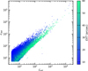 |
Fig. 1 Extent likelihood 𝓛ext and detection likelihood 𝓛det distribution of all extended sources. About 2% of the eRASSl X-ray source catalog, totaling up to 26 682 sources, are extended with EXT > 0. |
2.3 Optical identification of eRASSl clusters
This section briefly describes the optical identification process of eROSITA extended sources as clusters of galaxies. Details are provided in (Kluge et al. 2024). The optical identification is performed using the eROMaPPer algorithm (Ider Chitham et al. 2020), a highly parallelized version of the red-sequence matched-filter Probabilistic Percolation cluster finder redMaPPer (Rykoff et al. 2014, 2016), adapted for the identification of X-ray-emitting clusters and groups near eROSITA X-ray centroids. To identify overdensities of passive red galaxies around these locations, we utilize the public DESI Legacy Surveys Data Release North (LS DR9N) at Dec ≳ 32.5 deg and Data Release (LS DR10) at Dec ≲ 32.5 deg (Dey et al. 2019)5.
We begin with the 14 818 eRASS1 X-ray extended sources (𝓛ext > 3) within the LS footprint after applying the geometrical masking, as described above. Of these cluster candidates, we find optical counterparts for 12 554 using eROMaPPer. The algorithm calculates richnesses, optical centers, and other optical properties, as well as photometric cluster redshifts zλ for all optically identified clusters based on the colors of their member galaxies on the red sequence. For this task, we use LS DR9N and DR10 g, r, z filter bands and (in rarer cases) DR10 g, r, i, z filter bands in the photometric redshift range of zλ < 0.8. In contrast, for the high redshift range beyond zλ > 0.8, we use the LS DR10 g, r, i, z, W1 and (in rarer cases) g, r, z, W1, and LS DR9N g, r, z, W1 filter bands to measure the photometric redshifts more accurately.
As an alternative to the photometric redshifts, we use, when possible, more precise spectroscopic redshifts zspec and adopt literature redshifts zlit of matched clusters from public catalogs.
The best redshift zbest is then chosen using a prioritization scheme. The highest priority is assigned to zspec because it has the lowest uncertainty. The spectroscopic cluster redshifts are calculated using a compilation of public spectroscopic galaxy redshifts and a dedicated spectroscopic follow-up program with the Hobby Eberly Telescope (Balzer et al., in prep.). Photometric redshifts have the second-highest priority, while literature redshifts are only assigned to clusters without optical identification by eROMaPPer or with photometric redshifts outside of the red-sequence calibration range. We note a few exceptions to this prioritization scheme, described in Kluge et al. (2024). The red sequence in our follow-up algorithm eROMaPPer is not calibrated below redshifts z < 0. 05. The extended galaxies, members of nearby groups, and clusters are excluded in the LS photometry and, hence, are missing in our galaxy catalogs, which we utilize to calibrate eROMaPPer. In this redshift range, the clusters and groups are inspected visually, and their photometric redshifts are replaced with the redshifts found in the literature if they are more accurate (see Kluge et al. 2024, for further details).
In total, we optically identify 12 554 clusters and groups, of which 11 888 are in LS DR10 (98.25%) and 212 in the LS DR9N (1.75%) area. An additional 151 sources are matched with known cluster catalogs from the literature, and we include their red-shifts in the catalog. With these additional clusters, we identify 12 705 clusters and groups. Fig. 4 shows some example X-ray and LS DR10 images of clusters found using eROMaPPer at low, intermediate, and high redshifts. We note that the redshifts provided in this catalog are heliocentric.
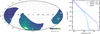 |
Fig. 2 Survey area and exposure information of the eRASSl cluster catalog. Left panel: vignetted exposure map in the 0.2–2.3 keV band after masking regions. The clean exposure time changes from ∼0.1 ks to 1.2 ks in the survey. Right panel: cumulative eRASSl sky coverage as a function of exposure in the 0.2–2.3 keV band. Blue solid and dashed curves show the data before and after cleaning. The curve in cyan shows the depth of the eFEDS survey, as a comparison (Brunner et al. 2022). |
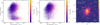 |
Fig. 3 Distance to the closest neighbor for each source is plotted against its ML_FLUX, demonstrating the general properties of the split sources on the sample level before and after cleaning on the right and middle panels. The color code denotes the extent likelihood 𝓛ext. Note the removal of the sources in the lower right corner. On the right panel, the figure shows an example of the split sources (dashed white circles) in a nearby cluster 1eRASS J115517.9+232422 at the redshift of 0.14. After cleaning, the source center is shown in a solid white circle. The circles in green are the point sources detected by eROSITA in the field. |
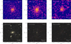 |
Fig. 4 Examples of eRASS1 clusters. From left to right: 1eRASS J120427.3+015346 (MKW4) at z = 0.020, eRASS1 J115517.9+232422 at z = 0.142, and eRASS1 J010257.4-491609 (El Gordo) at z = 0.869. The upper panels show eRASS1 X-ray image in the 0.2–2.3 keV band, smoothed with a Gaussian of σ = 12″. LS DR10 grz images are shown in the lower panels, overlaid with X-ray contours. |
2.4 Contamination estimation via a mixture model
Our realistic eRASS1 simulations (Seppi et al. 2022) show that identifying contaminants purely based on X-ray selection is challenging. We developed a mixture model that considers both X-ray and optical properties to estimate the overall contamination fraction in the eRASS1 cluster catalog. Bright AGN and spurious sources due to background fluctuations are expected to constitute most of the contamination in our X-ray extended source catalogs (Seppi et al. 2022). Additionally, on the optical side, line-of-sight projections and misidentification of stars as galaxies can lead to spurious overdensities of apparently red extended objects near the eRASS1 extended sources. The mixture model identifies contaminants on both X-ray and optical sides by comparing the distribution of redshift–richness–X-ray count rate properties of random sources (RS) and AGN to the distribution of the 12 705 clusters.
Random line-of-sight projections and the positions of spurious X-ray sources are expected to appear relatively homogeneously in the sky. The contribution of these contaminants is therefore determined by running eROMaPPer on one million random points in the LS footprint. We require these points to be at least five optical cluster radii D > 5Rλ away from the extended eRASS1 sources. Of the remaining ∼710 000 random points, we identify an overdensity of red-sequence galaxies in ∼250 000 cases and measure their photometric redshifts and richness. The other major contaminants, AGN mischaracterized as extended sources, are expected to reside in slightly more over-dense regions due to their clustering (Comparat et al. 2019). We estimate their contribution by running eROMaPPer on the X-ray centroids of ∼850 000 of all eRASS1 point source detections within the LS footprint. Of these sources, we find an identifiable red sequence with a measured photometric redshift and richness in ∼490 000 cases. With these distributions, we compute a contamination estimator Pcont as the ratio between the kernel density estimates of the probability P of random sources (RS), AGN, over cluster candidates (C). This procedure is repeated for all filter band combinations, and the contamination estimator is calculated for all of them independently before merging as a catalog. For the 291 clusters, for which the best redshift is adopted from the literature, we manually set their Pcont = 0.
The mixture model can then be expressed in the following form:
 (1)
(1)
where ƒRS and ƒAGN are the global fractions of contamination by random sources and AGN, respectively, and  are our set of observables, count rate, redshift, richness, and sky position.
This model expresses that the probability density function (PDF) for the measured observables of our sources is the sum of the PDF of the three different components: clusters, AGN, and random sources. The constant in front of each term represents the fraction of that kind of source; here, we note that ƒC = (1 – ƒRS – ƒAGN) is the cluster fraction. The PDFs are weighted so that when integrated over the entire parameter space, the total PDF is normalized to 1.
We can simplify the previous equation by dividing both sides by  the entire sample probability density, thus isolating optical richness, which is the quantity that truly allows the mixture model to disentangle the three populations in our catalog. Equation (1) becomes:
 (2)
(2)
where  and
and  are estimated using a kernel density estimator in our realistic eRASS1 simulations (Seppi et al. 2022), where we can identify precisely the different contaminants, while
  and
and  are obtained as specified above using eROMaPPer. Finally, we define Pcont as the ratio of the sum of the last two terms in Eq. (2) to the total probability. The total contamination fraction (ftot = ƒRS + ƒAGN) is used to calculate the purity of the sample (1-Pcont), which is given in Table 1.
Conceptually, this approach might look similar to the optical contamination estimators, which apply a simple redshift-dependent richness cut relying solely on optical data (e.g. Klein et al. 2019). The main advantage of our method is that it assigns a probability of being a contaminant that is informed by optically determined richness and redshift, as well as by the X-ray properties, namely, count-rate for each X-ray detection, including the candidate clusters and contaminants. Using X-ray information, which is not affected by the projection issues found with the optical data, helps keep clusters with low X-ray flux and low richness at higher redshifts in the sample. In traditional richness cleaning methods, these sources would be marked as contaminants and removed from subsequent catalogs. Our approach instead allows the user to decide on the preferred Pcont cut. In the primary eRASS1 cluster catalog, we provide the probability of being a contaminant for each source based on our mixture model. The Pcont cuts can be used to further clean the catalog based on the science application. In Table 1, we provide several selection criteria and the overall estimated purity in the samples after the cleaning is applied.
Cleaning through Pcont effectively suppresses the AGN contamination in the sample. Bright AGN, with high-count rates and low-richness values, are outliers in the richness versus count-rate parameter space and, therefore, have high Pcont values. The mixture model can identify the contaminants, for instance, the random association of background galaxies incorrectly associated with an X-ray source, as the majority of these cases will be outliers in the count-rate and richness scaling laws. These cases can be identified and removed efficiently by setting a Pcont cut. However, there are some instances where the mixture model cannot accurately estimate a detection’s Pcont value. In contamination fraction calculations, the count-rate easurements of random locations in the sky are chosen to be away from eRASS1 detected clusters. However, these locations may have extended sources just below our flux limit. Therefore, in these random locations, the count-rate measurements in the catalog, produced by the source detection algorithm, would be higher than the post-processed count rate measured by MBProj2D, our forward modeling tool for measuring cluster properties (see Sect. 5.1) after more careful treatment of the background. The mixture model’s kernel-density computed in our realistic eRASS1 simulations (Seppi et al. 2022) and the probability density function (PDF) of contaminants cannot be estimated accurately when the discrepancy between the MBProj2D count rate and the count rate in the catalog is significant. In these cases, the PDF values calculated from that combination of parameters approach zero. In the primary catalog, we find a small fraction of such cases (458 objects; 3.6%) by visually inspecting the sources where the discrepancy occurs. We remove these cases in the primary catalog by hand; see Sect. 3.1. Because of these caveats, we recommend users clean the cluster catalog with strict X-ray selection, for instance, 𝓛ext> 6 or 𝓛ext> 10, when employing the cluster catalog for population studies and cosmology.
The number of confirmed clusters with a set of selection on 𝓛ext and mixture model property Pcont.
3 Samples of clusters of galaxies and galaxy groups
3.1 The primary galaxy clusters and groups catalog
Our previous study based on the eFEDS survey shows that compact galaxy groups or high-redshift clusters with angular sizes comparable to the PSF of eROSITA may be classified as point rather than extended sources. The X-ray selection applied through 𝓛ext plays a vital role in keeping or excluding these sources in the cluster sample (see Bulbul et al. 2022, for details). Applying a high 𝓛ext cut in the X-ray selection process efficiently cleans the sample by removing the majority of contaminants, for instance, AGN, at the expense of removing many clusters (Seppi et al. 2022).
For example, in the eFEDS sample of 542 cluster candidates, an 𝓛ext threshold of 6 was adopted. Increasing this from 6 to 12 would remove ~60 contaminants and ~150 real clusters. Unless purity is a significant concern for a given scientific application, a practical solution to reach a higher purity and completeness level in the sample without losing many real clusters is to use the mixture model method described in Sect. 2.4. Here, we adopt a relatively low X-ray selection threshold for the primary cluster sample on 𝓛ext (namely, 𝓛ext > 3). This achieves higher completeness compared to an 𝓛ext> 6 sample like eFEDS, increasing the discovery space of eROSITA, while relying on the optical identification process confirmation to improve the reliability of the sample further (see Sect. 2.4). With this 𝓛ext threshold, we find 12 247 clusters of galaxies or galaxy groups after removing the 458 contaminants described above, mainly in the low-count regime and due to background fluctuations, and where the mixture model failed. The total effective survey area covered by this, which we designate as the primary eRASSl cluster sample, is 13 116 deg2 in the combined LS DR9N and DR10 footprint. The distribution of these clusters in the eROSITA sky is shown in Fig. 5. The number of clusters detected in the first All-Sky Survey is consistent with the pre-launch predictions (Merloni et al. 2012; Pillepich et al. 2012), demonstrating the superb performance of eROSITA.
Each cluster in the sample is identified by eROMaPPer or a literature redshift assigned to it and has an associated redshift measurement. We present the redshift distribution of the primary cluster catalog and the cosmology sample in Fig. 6. The redshift range, populated in the Zbest column in the catalog, spans from 0.003 to 1.32 with a median sample value of 0.31, slightly lower than the median redshift of 0.35 of the 477 clusters confirmed in the 140 deg2 eFEDS field (Liu et al. 2022). The reason for the lower median redshift of the two samples is twofold: eFEDS, although comprised of a small area, has higher exposure and hence greater sensitivity to high-redshift clusters. Secondly, the greater depth of the follow-up HSC survey, compared to LS and WISE surveys, has a significant impact on the identification of the higher redshift clusters.
In the catalog, the majority of redshifts (8790, 69%) are determined through photometric measurements. A large fraction of the sample (29%, 3510 clusters) of the sources have spectro-scopic redshifts, and 247 of the redshifts are from the literature (291 clusters with literature reshifts before visual cleaning) (see Kluge et al. 2024). The catalog includes 1451 nearby galaxy clusters and groups at z < 0.1, including well-known examples such as the Virgo, Fornax, and Centaurus clusters. Most of the sample, 10 074 (83%) galaxy clusters, and groups lie in the redshift range of 0.1 < z < 0.8. The sample comprises 722 clusters at high redshift z > 0.8. The highest redshift cluster, 1eRASS J020547.4-582902, is located at redshift 1.32 with 𝓛ext = 4.1, showing eROSITA’s capability to detect high redshift clusters. This cluster is cross-matched to a detection of a cluster in the Atacama Cosmology Telescope (ACT) DR5 catalog at the same redshift. Of the 12 247 clusters and groups in the primary sample, 8361, corresponding to 68% of the sample, are detected for the first time and are new discoveries. The remaining 3886 clusters can be found in other cluster catalogs in the literature. The details of cross-matching with published cluster catalogs in the literature are described in Sect. 4.
Located at the intersection of the cosmic filaments, the detection of a large number of massive galaxy clusters and groups with eROSITA can be used to extract information about the clustering pattern and to map the large-scale structure of the Universe. Historically, the local universe has been studied in detail by the galaxy surveys in the optical band, showing a number of large-scale patterns (Geller & Huchra 1989; Colless et al. 2001). The distribution of 97 952 galaxies in the GAMA and SDSS spectroscopic surveys in gray circles in Fig. 7 provide maps of the large-scale structures in the Universe (Driver et al. 2022; Almeida et al. 2023) – the filaments stretching several tens of Mpc can be seen in the figure. The galaxy groups and clusters located at the intersection of the cosmic web detected by eROSITA in the first All-Sky survey are shown in red circles. The apparent correlation between the location of the connecting knots of galaxy surveys and eROSITA detections demonstrates the potential of eROSITA in mapping the large-scale structure (see also Ghirardini et al. 2022; Liu et al. 2022). This correlation will become more apparent as the survey gets deeper and eROSITA detects a more significant number of low-mass group-size haloes as part of the large-scale structure. An accompanying paper by Liu et al. (2024) provides a catalog of superclusters and their member profiles.
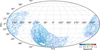 |
Fig. 5 The projected locations of the 2247 clusters and groups in the primary catalog in the eROSITA and LS DR9N and DR10 13 116 deg2 common footprints are shown. The detections outside the footprint with ∣b∣ < 15 deg are the redshiſts of the clusters added from the literature. The redshiſt confirmed by the follow-up algorithm eROMaPPer is color-coded (Kluge et al. 2024). |
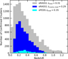 |
Fig. 6 Redshift distribution of the 12 247 confirmed eRASSl clusters and groups. Shown in gray is the eRASSl cluster sample with 𝓛ext> 3. compared to those of the cosmology sample in blue, and the redshift distribution of the 477 clusters confirmed in the eFEDS field in cyan (Liu et al. 2022). The median redshift of the eRASSl cluster catalogs is slightly lower than that of the eFEDS clusters (zmeđ = 0.35). |
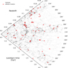 |
Fig. 7 Distribution of nearby eRASS1 galaxy clusters along the equator (red circles) illustrating the large scale structures of the Universe. Positions are projected along declination (|Dec| < 2 deg) within redshift 0.2. Galaxies from the GAMA and SDSS survey are represented with grey dots (Driver et al. 2022; Almeida et al. 2023). |
3.2 The cosmology sample
The selection methodology for our primary cluster sample emphasizes completeness over purity. Different samples can nonetheless be constructed with higher levels of purity by applying various cuts, for instance, in 𝓛ext or Pcont (see Table 1). Highly pure samples of clusters are more suitable for accurate determination of the cosmological parameters and testing of cosmological models. Here we describe the construction of the eRASS1 cosmology sample, which is used in the work of (Ghiradini et al. 2024) and the follow-up weak lensing mass calibration papers (Grandis et al. 2024; Kleinebreil et al. 2024).
We first select a sample with a stricter 𝓛ext threshold (𝓛ext> 6), resulting in 11 141 extended sources in the clean eRASS1 cluster catalog. This selection efficiently removes a large fraction of contaminants that are not true extended X-ray sources, such as AGN and background fluctuations. To ensure the uniformity of the optical identification process and to track any biases in the redshift measurements, we use only the LS DR10 region and exclude the LS DR9N area. Specifically, we limit our area to uniformly processed LS DR10-South region with Dec ≲ 32.5°. This limits the survey area to 12 791 deg2. Within this LS DR10-South footprint, at 𝓛ext > 6, there are a total of 8129 extended X-ray sources. Of these, eROMaPPer is able to identify 7077 candidate clusters in the LS DR10-South footprint by combining g, r, and z filter bands to ensure homogeneity of the richnesses, redshifts, and contamination estimation. Of the 7077 candidate clusters in the LS DR10-South footprint, we can identify the optical counterparts of 6562 securely detected clusters.
To select only clusters with photometric redshift lower than the limiting redshift at that sky position, we apply the flag IN_ZVLIM==True (see Kluge et al. 2024, for further details). For the excluded clusters due to the limiting redshift cut, the detection of faint galaxies just above the limiting luminosity L > 0.2 L* of the corresponding Legacy surveys becomes uncertain, and the measured richness artificially increases because of Eddington bias (Kluge et al. 2024). As weak lensing mass bias calculations rely on the richness values (see Grandis et al. 2024, for further details), we limit our sample to a regime where the member selection is most reliable. Furthermore, the photometric redshift range is kept limited to 0.1 < z < 0.8, where the photometric redshifts are the most reliable (see Kluge et al. 2024, for details). The final cosmology sample comprises 5259 galaxy clusters in the 12 791 deg2 LS DR10-south area. The redshift distribution of the sample is displayed in Fig. 6 with a sample median of 0.29, slightly lower than the primary cluster catalog due to the elimination of high redshift sources.
3.3 Purity and completeness
To compute the completeness of the sample, we use the digital twin of eRASS1 the details of which are described in Seppi et al. (2022). We briefly summarize the main characteristics here. In the digital twin, a dark matter halo light cone extending to redshift six is generated from the UNIT1i simulation (Chuang et al. 2019). The X-ray emission is predicted using accurate models of AGN and cluster emissivity from Comparat et al. (2019, 2020). The X-ray background is generated by resampling the actual eRASS1 data. X-ray events are generated with the SIXTE simulator (Dauser et al. 2019) with the ancillary response file (ARF), the redistribution matrix file (RMF), and the attitude file of the spacecraft in the eROSITA Data Release 1 calibration database consistently. We match the resulting source catalog to the input catalog by tracing the origin of each photon. The sources are grouped into several classes. A source with a primary counterpart of a simulated point source (AGN or a star) or a simulated extended source (cluster) is included in the catalog. Additionally, sources that are secondary counterparts of simulated point sources or extended sources are also added to the catalog. We also consider false detections due to random background fluctuations, where the source catalog entry is not associated with any simulated source.
Figure 8 shows the completeness and number of clusters as functions of flux limit for two 𝓛ext thresholds: 𝓛ext >3 (black) and 𝓛ext > 6 (blue). X-ray-selected samples can reach high completeness levels when higher flux cuts are applied. For instance, above the flux limit of 8 × 10⁻¹³ ergs s−1 cm−2, the primary cluster catalog has a completeness level of ∼90%; however, the number of clusters (∼1300) above that flux is relatively low. Choosing a lower flux limit of 4 × 10⁻¹⁴ erg s−1 cm−2 would increase the sample size to > 10 000 while the completeness declines to a level of 13.3% in the primary sample (𝓛ext > 3 selection). The cosmology sample with (𝓛ext > 6), above the flux limit of 10−13 erg s−1 cm−2, has a completeness of ∼30%. In general, the trade-off between completeness, purity, and the number of clusters should be decided based on scientific application.
We compute the sample’s purity by integrating the clusters’ Pcont values (see Table 1). Based on our estimates with the mixture model, the primary cluster catalog with 12 247 sources in the 13 116 deg2 survey area has a purity level of 86%. Applying either higher X-ray and optical selections through Pcont or both would further reduce the contamination of this sample. For instance, selecting clusters with a lower probability of being a contaminant, namely, Pcont < 0.5, removes most of the contamination in the sample, leaving 10 865 clusters with a sample purity level of 95% (see Table 1). Applying higher thresholds in the X-ray selection, for instance, 𝓛ext > 6, produces samples with 94% purity in the cost of removing 5495 extended sources. Increasing the 𝓛ext threshold to 10 removes the majority of the contamination and produces highly pure samples at > 98% purity level with a sample size of 4171. Above the X-ray 𝓛ext > 10 threshold, X-ray selection is so efficient that additional optical selection is unnecessary.
The cosmology sample optimized for high purity with a different set of X-ray (𝓛ext > 6) and optical selections has 5259 clusters candidates in the LS DR10 survey area of 12 791 deg2 and has a purity level of 95%. Applying Pcont < 0.5 cut increases the purity level to 97%, leaving 5087 securely confirmed clusters in the sample. X-ray selection is a more reliable way of cleaning samples than optical selection as projection effects impact X-rays less; we recommend users apply stricter X-ray selections, for instance, 𝓛ext > 10 or 15, when necessary to generate purer cluster samples.
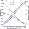 |
Fig. 8 Completeness as a function of intrinsic unabsorbed flux limit for two 𝓛ext thresholds: the cluster catalog 𝓛ext > 3 (in black) and the cosmology sample 𝓛ext > 6 (in blue). The dashed curves show the corresponding number of clusters for both samples. The trade-off between completeness and the number of clusters in the primary cluster sample is clear in the figure. |
4 Comparisons with overlapping cluster surveys
In this section, we provide the counterparts of eRASS1 clusters found in several previously published cluster catalogs compiled from X-ray, SZ, and optical surveys. The matching radius we use for this work is set to 2′; this radius is ideal for identifying close associations for eROSITA. Using larger matching distances causes the clusters to be associated with the surrounding large-scale structure, for instance, infalling haloes, for most surveys, except for the Planck survey as demonstrated in Bulbul et al. (2022). The identifiers of the matched clusters are given in the catalog under the column “Match Name”. In total, we find 3886 clusters have counterparts in various cluster catalogs. 68% of our sample, a total of 8361 clusters, are not matched with any other “optically confirmed” source in the published catalogs. Therefore, they are newly discovered clusters. If we only consider clusters in X-ray and SZ catalogs, namely, ICM-based catalogs, then 9795 clusters corresponding to 80% of the eRASS1 cluster sample are detected and identified for the first time. We calculated the purity level of the new detections in the primary sample to be 81%, whereas the newly discovered clusters in the cosmology sample have a purity level of 92%. We provide the details of the matched catalogs and the overlapping area with eROSITA Western Galactic Half in the following subsections. A summary of the results and the distribution of redshifts of the cross-matched samples are given in Table 2 and Fig. 9. For comparisons, we over-plot the redshift histogram of the newly discovered eRASS1 clusters in the figure. For eRASS1 clusters, we use the zbest in the histogram.
4.1 Surveys in the X-ray band
The first true imaging all-sky survey in the soft X-ray band was performed by ROSAT in the period of 1990–1991 (RASS, Voges et al. 1999). The RASS was shallower and had a worse angular resolution, with the half-power radius being 84″ (Boese 2000), compared to the eROSITA All-Sky Survey. Nonetheless, many of our clusters were already discovered with ROSAT. Several sub-catalogs have emerged over the past two decades. The ROSAT ESO Flux Limited X-ray Galaxy Cluster Survey (REFLEX, Böhringer et al. 2004) was compiled in a region with a declination of ≤+2.5 deg and excluding the Milky Way via a Galactic latitude cut of ≤−20 deg in the southern sky, consequently covering a survey area of 13 924 deg2 down to a flux limit of 3 × 10⁻¹² erg s−1 cm−2. A total of 441 clusters of galaxies are confirmed in the REFLEX catalog. The Northern ROSAT All-Sky galaxy cluster survey (NORAS, Böhringer et al. 2000) was based on RASS data excluding the same region around the Galactic plane but covering the northern sky. In this catalog, 437 clusters were confirmed based on a combination of count rate (>0.06 cts s−1 in the 0.1–2.4 keV band) and a source extent likelihood. Another cluster catalog that was based on RASS is the ROSAT Brightest Cluster Sample (BCS; Ebeling et al. 1998), consisting of 201 X-ray-brightest clusters of galaxies in the northern hemisphere (δ ≥ 0 deg), at high Galactic latitudes of |b| ≥ 20 deg. Cluster surveys with more limited area but greater depth have also been performed with ROSAT. For instance, Cruddace et al. (2002) performed a cluster survey in a region of 56 deg2 around the South Galactic Pole, down to a flux limit of 1.5 × 10⁻¹² erg s−1 cm−2. The 400 Square Degree ROSAT PSPC Galaxy Cluster Survey (Burenin et al. 2007, 400SD) covered an area of 397 deg2 with high Galactic latitude |b| > 25 deg with a flux limit of 1.4 × 10⁻¹³ erg s−1 cm−2. All these ROSAT catalogs were compiled by Piffaretti et al. (2011) into a meta catalog of 1743 confirmed clusters, with which we cross-match the coordinates in our catalog (RA, Dec) with 2′ matching radius. We apply the same procedure to match the subsequent catalogs.
The MCXC survey has the largest area in common with eRASS1 due to its full sky coverage; the cross-match results in 588 clusters in a sample of 681 clusters in the common footprints of both surveys. The cross-matched sample has a sample median redshift of 0.11. The median centroid offset is 3l″.6, consistent with eROSITA and ROSAT’s PSF size.
The CODEX (COnstrain Dark Energy with X-ray clusters Finoguenov et al. 2020) sample is also based on the ROSAT All-sky Survey, identifying 10 382 X-ray sources with red sequence counterparts in the 10382 deg2 SDSS area reaching down to an X-ray flux limit of 10−13 ergs s−1 cm2. The majority of the CODEX survey area is in the northern sky with a limited common footprint with eROSITA in 3508 deg2. Of the 3106 objects in the CODEX catalog, we detect and confirm only 574 of these sources, with a median redshift and offset of 0 22 and 50″.2. The large offset between the ROSAT based MCXC and eRASS1 sample, still within the PSF size of ROSAT, could be due to the different detection algorithms, namely, wavelet filtering, employed to detect clusters. The MARD-Y3 catalog, on the other hand, is constructed from the DES-Y3 gold catalog using the priors from the ROSAT All-Sky survey catalog (Klein et al. 2019) – the cross-match results in 904 associations with a median redshift of 0.23. The low matching rate may indicate a large contamination level in the CODEX and MARD-Y3 catalogs based on shallower ROSAT data. It is worth noting that CODEX and similar catalogs, such as MARD-Y (Klein et al. 2019) and RASS-MCMF (Klein et al. 2023), are constructed based on the X-ray catalog with no extent selection and no ICM selection; therefore, they are subject to higher levels of contamination and significant optical selection effects. The significance of this catalog is that we provide an initial selection of the extent likelihood in X-rays that significantly reduced the contamination in the sample.
RXGCC is one of the most recent catalogs based on the ROSAT data, performed with a wavelet-based detection algorithm and strict extension likelihood (>25) and extent (>0′.67) selection, includes clusters down to flux of 2.49 × 10⁻¹² erg s−1 cm−2 (Xu et al. 2022). This catalog is optimized to find very extended groups missed in the previous ROSAT catalogs. We find 256 of their most nearby groups and clusters (zmed = 0.08) in our sample, with a large centroid offset of 55″.2, consistent with the other ROSAT samples. The larger offsets are likely due to the considerable of these clusters and groups.
Deep X-ray surveys focused on scanning smaller areas have been performed with XMM-Newton, resulting in cluster catalogs reaching lower flux limits than ROSAT. Most relevantly, in the 50 deg2 XMM-Newton XXL survey with roughly 10 ks exposure time, a total of 365 clusters are detected down to flux limits of 10−15 erg s−1 cm−2 (Pierre et al. 2016; Adami et al. 2018). Of these 365 clusters, 11 are detected in eRASS1 observations with a small central offset of 14″.1. The median redshift of the cross-matched sample is consistent with the median redshift of the XXL sample. Other relevant XMM-Newton surveys include the XMM-Newton Cluster Survey (XCS, Mehrtens et al. 2012) and XMM-Newton Cluster Archive Super Survey (X-CLASS, Koulouridis et al. 2021), consisting of 503 and 1559 optically confirmed galaxy clusters detected using XMM-Newton archival data. Of the 1559 clusters in the X-CLASS sample, 304 have eRASS1 counterparts, with a median redshift of 0.14. XCS has 36 close associations in eRASS1. The median centroid offset, ~17″, is well within the eROSITA survey averaged PSF and consistent with other XMM-Newton surveys. In general, the clusters observed with XMM-Newton have small offsets with respect to their eRASS1 counterparts, which is not surprising given the 6″ FWHM PSF of XMM-Newton and ~5″ localization accuracy of eROSITA (Brunner et al. 2022)6. Although the number of eROSITA counterparts of the clusters detected in XMM-Newton surveys seem to be small in number due to the shallower survey depth and slightly worse angular resolution of eROSITA, the size of the cross-matched sample will increase as eROSITA survey gets deeper. The main advantage of eROSITA based cluster surveys is the large and contiguous area coverage compared to the XMM-Newton data.
The first survey of eROSITA is the eFEDS, which covered a 140 deg2 region in the Equatorial strip, with approximately 10× deeper exposure than eRASS1. In the eFEDS field, we confirm 477 of the 542 cluster candidates with 𝓛ext> 6. We find 63 common detections with a median redshift of 0.29. The details of the detection probabilities of these commonly detected clusters are provided in Clerc et al. (2024). The median offset is 17″.1, most likely caused by high Poisson shot noise due to the low exposure time of eRASS1. We make in-depth comparisons of X-ray properties of eFEDS clusters with eRASS1 in Sect. 5.4.
Public Cluster Catalogs Cross-matched with eRASS1.
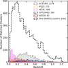 |
Fig. 9 Redshift histogram of the matched eRASS1 clusters in the ROSAT, Planck All-Sky Surveys, ACT, and SPT-SZ surveys and the newly discovered eRASS1 clusters. The redshifts indicated here are adopted from the literature catalogs that are matched. For the eRASS1 catalog, zbest is used in the histogram. The largest overlap of clusters (1176) is between RASS and ACT DR5 surveys due to the large common area between the two surveys with eROSITA. |
4.2 Sunyaev Zel’dovich effect surveys
Another efficient way of detecting clusters through their ICM emission is by searching for the SZ effect signatures in the cosmic microwave background. The SZ effect signal is independent of redshift, making SZ surveys sensitive to clusters at higher red-shifts. A few independent ground- and space-based SZ cluster catalogs have become available in the last decade. However, due to their wide beam sizes or limited area coverage, the catalogs of extended sources remain limited to a few hundred to a few thousand clusters. Specifically, we compare our catalog with those from the Planck satellite, ACT, and the South Pole Telescope (SPT).
Planck, launched in 2009, assembled its final All-Sky cluster catalog of 1653 sources in 2016. The eROSITA primary cluster catalog presented here and Planck have 10 281 deg2 common footprint area with 439 counterparts in our catalog with a median sample redshift of 0.21. Planck detected clusters show the largest offset with the eROSITA counterparts compared to other surveys cross-matched with our primary cluster catalog; this is most likely due to the large beam size (9′.65 at 100 GHz Planck Collaboration VII 2014).
The ACT DR5 catalog consists of 4500 clusters of galaxies collected from the runs of the ACTPol survey between 2008 and 2018 in the 13 211 deg2. The sample is mass-limited with a high completeness level of 90% and a signal-to-noise ratio (S/N) threshold of > 4σ. However, the false detection rate can be as high as 30% in this sample (see Fig. 6 in Hilton et al. 2021). When the (S/N) > 5σ selection is applied, the contamination fraction in their catalog drop to a few percent. Regardless, we provide the eRASS1 counterparts of all detections reported in their catalog for completeness. ACT has a smaller beam size than Planck; therefore, it is more sensitive to detecting clusters at higher redshifts. This is reflected in the cross-matched sample’s median redshift (zmed = 0.41). ACT has the largest number of associations with eRASS1: 1176 common clusters in the 6877 deg2 common footprint. Of these common clusters, 81 are at high redshifts (z > 0.80). Three of the highest redshift clusters in the eRASS1 catalog (1eRASS J020547.4-582902, J064017.1-511255, J015608.9-554159) are matched to ACT counterparts of ACT CL J0205.7-5829, ACT-CL J0640.2-5113, ACT-CL J0156.1-5542 with spectroscopic redshifts of 1.32,1.32, and 1.28, respectively. We find an agreement for these clusters in our spectroscopic and photometric measurements. One of our highest redshift clusters, 1eRASS J044237.2-590529, has a counterpart in the ACT catalog (ACT-CL J0442.6-5905) with a relatively small angular separation of 1ľ/7. However, the photometric redshift reported in Hilton et al. (2021), zλ = 1.48 ± 0.035, is in disagreement with our bias-corrected photometric redshift measurement of  based on LS DR 10 g, r, z, W1 data.
The SPT, a 10-meter diameter telescope located at the South Pole Station, has performed deeper surveys in a more confined area than ACT in the western Galactic half of the sky. The first SPT survey, SPT-SZ hereafter, covering a region of 2500 deg2, was completed in 2011. The sample based on SPT-SZ data comprises 516 confirmed clusters with a detection significance of 4.5σ (Bleem et al. 2015; Bocquet et al. 2019). Another survey performed with the upgraded SPT-pol receiver covers a 100 deg2 area. The survey catalog contains 89 candidates detected with a signal-to-noise ratio > 4.6, 81 confirmed via optical and infrared follow-up observations (Huang et al. 2020). Later, the SPT-pol receiver was used to scan a larger area in 2013, 2014, and 2015, covering a 2700 deg2 region. In the SPT-pol Extended Cluster Survey (SPT-ECS), a total of 470 optically confirmed clusters are reported down to a signal-to-noise >4 (Bleem et al. 2020). We find 353, 241, and 21 counterparts in the eRASS1 catalog with mean redshifts between 0.38 and 0.44 and centroid offsets between 16″ and 21″, comparable to ACT centroid shifts.
4.3 Optical surveys
Surveys executed in the optical band results in large catalogs of galaxy clusters. We compare our X-ray cluster sample with the following catalogs of optical galaxy concentrations: Abell, GOGREEN, DES, Wen & Han, and MaDCoWS. The Abell catalog contained 1059 nearby rich clusters with redshift measurements (Abell et al. 1989; Andernach 1991); 466 are in our eRASS1 footprint. We find only 152 clusters in our catalog within 2′ of these Abell clusters. The low matching fraction is partly due to the misclassification and projection effects in the Abell catalog (van Haarlem et al. 1997). One of the largest cluster catalogs compiled through the RedMaPPer algorithm is from the DES-Y1 data (McClintock et al. 2019). We find 781 close associations in our catalog with DES-Y1 clusters with amedian sample redshift of 0.38 and a median separation of 17″.6. One likely reason for the low matching ratios between eRASS1 and optical catalogs, such as the Abell catalog, is the offset between the centering of the optically selected clusters. The offset between the X-ray centroid and optical centers is often larger than our matching radius of 2′. 1eRASS J103943.5-084115 at a redshift of 0.08 is a good example for this case. The optical centroid of A1069 is 6′ away from the eROSITA cluster center, although the match is clear due to the agreement in redshifts between two catalogs. Additionally, the limited red-sequence calibration (z > 0.05) and flagged LS DR10 photometry for very extended galaxies makes the identification of low-redshift eRASS1 clusters (z < 0.05) difficult, leading to incomplete eRASS1 catalog in this redshift regime. The identification process and limitations are explained in detail in Kluge et al. (2024).
The eROSITA cluster catalog has a significant number of detections at high redshifts z > 0.8. At these redshifts, optical identification through red sequence cluster finding tools in g, r, i, z, W1 bands becomes challenging due to the limited depth of the LS. Dedicated infrared cluster surveys are helpful in the identification of high-redshift candidate clusters. Wen & Han (2018) compiled a catalog of 1959 high redshift clusters in the redshift range of 0.7 < z < 1.0 based on the SDSS and Wide-field Infrared Survey Explorer (WISE). The common area of this survey with eRASS1 is small, but we detect 10 of their high redshift clusters. GOGREEN (Gemini Observations of Galaxies in Rich Early ENvironments) and GCLASS (Gemini CLuster Astrophysics Spectroscopic Survey) surveys selected a sample of the Spitzer Adaptation of the Red Cluster Sequence (SpARCS) Survey (Balogh et al. 2021; Wilson et al. 2009), and SPT clusters in the redshift range of 0.8 < z < 1.5, and have spectroscopically confirmed 26 clusters in this redshift range. The eRASS1 sample has two close associations with this sample (Bleem et al. 2020). Another high redshift cluster survey is based on the data from the WISE mission, the Massive and Distant Clusters of the WISE Survey (MaDCoWS) (Gonzalez et al. 2019). Its main goal is to find galaxy clusters at 0.7 < z < 1.5. We find 12 clusters in common associations in eRASS1. In the near future, the combination of Euclid and eROSITA surveys will help confirm the majority of the eROSITA high redshift candidates with the inclusion of Y, J, and H bands in the eROMaPPer pipeline and open this attractive redshift regime for the structure formation studies.
5 X-ray properties of the eRASS1 galaxy clusters and groups
One of the main goals of this paper is to provide X-ray properties of the clusters and groups detected in eRASS1. The initial source properties provided in Merloni et al. (2024) help define the sample, but quantities such as count rates and fluxes supplied by the source detection algorithm are only very rough estimates for clusters. Here, we improve them using more precise measurements, taking into account the corrections for Galactic absorption, K-factor, and a more accurate ICM and background modeling.
5.1 Post-processing of the eROSITA data
Further X-ray analysis of the eRASS1 clusters is performed using the MultiBand Projector in 2D (MBProj2D) tool (Sanders et al. 2018). MBProj2D (Appendix A) is a code that forward-models background-included X-ray images of galaxy clusters to fit cluster and background emission simultaneously. During this process, a Markov chain Monte Carlo (MCMC) analysis is used to generate profiles of cluster physical quantities. Besides using a forward modeling approach, the main advantage of MBProj2D is that the code allows simultaneous and self-consistent modeling of the surface brightness and temperature information and easier visual inspection for the goodness of the fit and background modeling.
Given a sufficient number of energy bands, MBProj2D can provide equivalent results from spatially-resolved spectral fitting, such as radial profiles of density, temperature, and metal-licity. In recent work, MBProj2D is applied to the deepest eROSITA data currently available (eRASS:5) of the galaxy cluster SMACS J0723.3–7327 (Liu et al. 2023), showing good performance. The X-ray properties determined using MBProj2D are provided in both catalogs, primary cluster catalog and cosmology sample; see Table 3.
Our MBProj2D analysis of the eRASS1 clusters is summarized as follows. We use images in multiple energy bands for the analysis to help constrain the ICM temperature. Specifically, for each cluster, we create images and exposure maps in the following energy bands (in units of keV): [0.3–0.6], [0.6– 1.0], [1.0–1.6], [1.6–2.2], [2.2–3.5], [3.5–5.0], [5.0–7.0], using the evtool and expmap commands in eSASS. The image size is 8 R500 × 8 R500, which is large enough to include a local background region beyond the cluster. The initial R500 adopted to determine the image size is a rough estimate using the L – M scaling relation for eFEDS clusters (Chiu et al. 2022), where the luminosity is estimated measured from the eROSITA X-ray data, and mass is measured from the weak lensing signal. A superior estimate of R500 is provided later from the cosmology analysis (see Sect. 5.2), but we note that the fitting of the cluster properties is not very sensitive to the precise size of the image. Faint point sources with ML_RATE < 0.4 in the 0.2– 2.3 keV band within the image are masked, while brighter ones are fitted to ensure that the emission due to the outer wings of the PSF is properly modeled. This follows the approach adopted by Ghirardini et al. (2022). PSF and ARF variations across different bands are adequately considered by creating separate response files for each band. In the fitting process, we allow the central coordinates of the source to vary to enable more accurate measurements of the X-ray peak of the surface brightness of each cluster. We present the offset between clusters’ initial coordinates provided by the source detection chain (RA, Dec) and the refined coordinates obtained from the MBProj2D processing, namely, (RA_XFIT, DEC_XFIT) in the left panel of Fig. 10. The median offset of 7″.7 is consistent with the 2σ range of the localization uncertainties of eROSITA (Brunner et al. 2022). There is a sharp drop in the distribution of offset values larger than 10. However, we observe a relatively large offset in a small fraction of the sample. This large offset is often due to the cleaning of ‘split’ sources in the eRASS1 catalog (see Sect. 2 for the details of the cleaning procedure) and the improvement in the background subtraction and modeling of the ICM emission. In the post-processing with MBProj2D, a more accurate background estimate is performed using a local region extracted around the cluster, with a more rigorous point source excision process. In contrast to MBProj2D, the background map created by the source detection process may still include emission from bright point sources due to the wings of PSF or ICM emission in cluster outskirts, as the extended sources were excised within their extent (EXT) values in the creation of the background map. Additionally, we use a more flexible ICM electron density model with more free parameters than the β profile with a fixed slope assumed during the source detection process. Therefore, the X-ray centers determined in our post-processing analysis are more accurate and are used in our cosmology and scaling relation analyses (Ghiradini et al. 2024; Grandis et al. 2024).
We use the electron density profile from Vikhlinin et al. (2006), but without the second β component, which is not needed in our fits as most of the X-ray emission comes from the core region of the cluster:
 (3)
(3)
The electron and proton densities are represented by ne and np, and we assume ne = 1.17np (Bulbul et al. 2010). γ is fixed at 3. n0, rc, α, β, rs and e are free parameters.
For each cluster, the MCMC chain produces posterior distributions of free parameters, such as the X-ray center, ICM temperature (kT), and electron density model (ne(r)). X-ray properties such as flux and luminosity as functions of radius and energy bands are then derived from the chains. Most of the eRASS1 clusters we analyzed in this work have fewer than a few hundred counts. Therefore, we do not attempt to constrain the 1D temperature variation but assume a constant temperature throughout the cluster. Metal abundance is fixed at 0.3Asun due to the limited number of photons. The adopted solar abundances are from Asplund et al. (2009). We use the HI4PI survey self-consistently to compute the Galactic neutral hydrogen column density throughout the analysis (HI4PI Collaboration 2016). We note that most of the confirmed clusters in our sample have relatively low nH because they are located at high Galactic latitudes. Therefore, the effects of equivalent total hydrogen column density absorption in our results are negligible. Allowing nH free to vary or adopting the total hydrogen density nH,tot (Willingale et al. 2013) does not change our measurements significantly. Due to the shallow nature of the survey, we are limited by the low number of counts in our analysis. Therefore, we use C-stat as the estimator for the goodness-of-the-fit to avoid any biases on the best-fit parameters (Kaastra 2017). The physical properties of the clusters are computed at zbest.
The offset between the fitted X-ray center and the brightest clusters galaxy (BCG) can be used to trace the dynamical state of a cluster (e.g., Hudson et al. 2010; Rossetti et al. 2017; Seppi et al. 2023; Ota et al. 2023). Shown in the right panel of Fig. 10 is the projected separation of the X-ray (RA_XFIT, DEC_XFIT) and the BCG coordinates given in (RA_BCG, DEC_BCG; Kluge et al. 2024). We convert the angular separation into physical scales (kpc) following the procedure described in Seppi et al. (2023), using the zbest column. The eRASS1 cluster sample with 𝓛ext > 3 shows a median offset of 178 kpc. Selecting a more secure sample Pcont < 0.5 (see Table 1) yields a very similar sample median offset of 179 kpc. Most of the eRASS1 clusters have an offset smaller than ∼200 kpc, while a significant tail extending to several hundred kpcs and a slight excess around 1000 kpc can be observed in the distribution. We further cleaned the distribution by selecting galaxies based on their probability of being the BCG of the cluster (PBCG; see Kluge et al. 2024, for the probability PBCG measurements). The elimination of the galaxies that are less likely to be the BCGs, with a selection of the probability PBCG < 0.7, removes many of the sources with large offsets (see Fig. 10) and brings the sample median to 127 kpc (22″). The clusters with large offsets are likely more disturbed, as pointed out in Seppi et al. (2023). Detailed analysis of the morphology and dynamical status of the eRASS1 clusters will be performed in another work (Sanders et al., in prep.).
In Fig. 11, we show examples of X-ray products for an example cluster (1eRASS1 J115517.9+232422). On the leftmost panel, the soft band image of the cluster is shown after the point sources in the field are excluded. The second panel to the left shows the residual noise image after the cluster emission is modeled. These images show that our analysis method can adequately model the emission from the contaminants and cluster itself. Visual inspections suggest that no excess emission is found in the residual plots of the eRASS1 clusters. The two rightmost panels show the luminosity and electron number density profiles of the same cluster with the 68% confidence intervals displayed in shaded regions. We note that the shallow nature of the survey does not allow us to make number density measurements at large radii, which is clear from the size of the uncertainties. The figure shows the extrapolations of the best-fit models in these regions.
We also show the electron density profiles and luminosity profiles for all the clusters in the primary 𝓛ext > 3 sample, after rescaling with R500, which are plotted in Fig. 12. The median of the profiles is plotted in violet, with the 16 and 84 percentiles shown in shaded regions. The figure on the left panel shows that the sample consists of both cool-core clusters with high central density and non-cool-core clusters with flatter central profiles. The evolution and universal behavior of profiles will be discussed in the follow-up papers by Bahar et al. (in prep.) and Moysan et al. (in prep.)
Description of the Columns in the Primary Cluster Catalog FITS File.
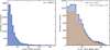 |
Fig. 10 Offset between the coordinates in the eSASS detection chain (RA, Dec) and the coordinates after post-processing of the data by MBProj2D (RA_XFIT, DEC_XFIT), shown on the left panel, have a small median value of 7.7″. The tail of the distribution is due to the split extended sources in the eSASS catalog, cleaned carefully in this work. The offset between the coordinates indicated by the MBProj2D and the BCG coordinates reported in Kluge et al. (2024) are presented on the right panel. The median offset between the X-ray center and BCG is 179 kpc for the full sample and 127 kpc after applying the selection PBCG > 0.7 to the sample, selecting secure BCGs. Large offset values are an indicator of the merger status of clusters. |
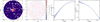 |
Fig. 11 Example of MBProj2D analysis and results. The left panels show the 0.2–2.3 keV image of eRASS1 J115517.9+232422 and the residual image after MBProj2D fitting. Point and extended sources are masked from the image. The noise level in the residual image shows that the source emission is successfully modeled from the fitting process. The right panels are the luminosity profiles and electron density profiles. |
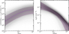 |
Fig. 12 Luminosity (left panel) and electron number density (right panel) profiles of the eRASS1 clusters shown in gray curves. The dashed curve shows the median profile with the 84th and 16th percentiles plotted in shaded regions. |
5.2 X-ray properties of eROSITA clusters and groups
In the primary catalog, we provide the X-ray properties, including the total number of counts, count-rate, flux (FX), luminosity (LX), temperature (kT), YX integrated over two radii (300 kpc and R500) in two energy bands (0.2–2.3 keV and 0.5–2.0 keV) obtained from the runs with MBProj2D. After obtaining the mass estimates, R500 measurements are calculated by  · The method used to calculate the total mass (M500) is described in the following section. The critical density, ρc, is calculated at the cluster’s redshift using the best-fit cosmological parameters from the eROSITA cluster count measurements (see Ghiradini et al. 2024).
In cosmological analyses utilizing cluster counts, it is essential to establish a mass calibration with scaling relations between the selection observables and cluster mass. The X-ray observable count rate offers a convenient mass proxy to describe a selection, which also has a well-established scaling with the halo mass (see Ghiradini et al. 2024). However, the observable must reflect each cluster’s intrinsic count rate; therefore, a similar X-ray reprocessing procedure must be applied to the cosmology sample. To estimate the intrinsic count rate of each source, the X-ray background must be treated carefully, and the Galactic column density (NH) and K-factor corrections must be accounted for. The only distinguishing component of this analysis is that the count rate measurements must be done at the photometric redshifts consistent with the cosmology sample, as justified in Sect. 3.2. Therefore, the only observables computed for this sample are the count rates within R500. From hereon, we will present the properties of the primary 𝓛ext>3 cluster sample.
The shallow nature of the survey limits the number of X-ray counts collected within R500 of each cluster. The count distribution in the 0.2–2.3 keV band of eRASS1 clusters is displayed in Fig. 13. eFEDS counts in the same band are also shown in the figure as a comparison. In the eRASS1 sample, only a tiny fraction (148 clusters; 1.2% of the sample) of clusters or groups have X-ray counts >1000, and they are primarily nearby clusters and groups. About 1892 clusters (15.5% of the sample) lie in the 100-1000 count range. The majority of the sample, 10 207 clusters (83.3%), have less than 100 counts.
The commonly inferred physical property from X-ray imaging observations of galaxy clusters is the band averaged luminosity within a characteristic overdensity radius R500. Ultimately, each cluster in the sample with a reliable redshift measurement has such a luminosity measurement. However, we only plot in Fig. 14 to the left the luminosity measurements with significant measurement, namely, at a > 2σ confidence level, and exclude upper limits for display purposes. As a reference, we also show as a dashed line the estimated flux in the 0.2–2.3 keV band of 4 × 10⁻¹⁴ erg s−1 cm−2. Unlike previous ROSAT cluster catalogs, we do not make flux cuts on the cluster sample since the eRASS1 survey depth is not uniform across the sky, and the eROSITA cluster survey is not a flux-limited survey. This effect is apparent in Fig. 14 (right panel); the flux of the detected and identified clusters is a function of the depth of the survey. The dashed line nonetheless provides a rough estimate of the flux limit of the survey.
The sample spans more than four orders of magnitude in luminosity, ranging from 1.1 × 1041 ergs s−1 to 3.6 × 1045 ergs s−1. The X-ray brightest cluster in the eROSITA sky is 1eRASS J010257.4-491609, a.k.a. El Gordo, at a redshift of 0.86, followed by 1eRASS J134730.8-114510 at a redshift of 0.45. About 84% of the sample (10 410 clusters) has a luminosity measurement at the > 2σ confidence level or more. The most luminous 1% of the sample, comprising 104 clusters, has luminosities larger than 8 × 1044 erg s−1, while 3138 (25.6%) of the sample lies in the faint end with luminosities LX < 1 × 1043 erg s−1. The majority of the clusters, 73.5% of the sample, lie between those two values. Most of the high-z clusters have high luminosities above 1044 erg s−1 and low 𝓛ext values <10, which is expected since we adopt a relatively low cut on 𝓛ext, to keep the high-z clusters in the eRASS1 cluster sample, and rely on optical cleaning to remove AGN and other contaminants. Only bright and massive clusters are detected at high redshifts due to the ‘Malmquist bias,’ inherent in all flux-limited surveys (Malmquist 1922). The decrease in the number of bright clusters detected at low redshifts reflects the shrinking survey volume in the nearby Universe.
Naturally, due to the shallow nature of the survey, the small number of counts per cluster is insufficient for reliable direct temperature measurements. To quantitatively evaluate the reliability of temperature constraints for the sample, we examine the MCMC chain for each object. We compute a histogram of kT points using 100 bins equally distributed in a logarithmic space from the minimum to the maximum point values in the chain. The computed histogram is an approximation of the marginal posterior distribution of temperature. We first calculate the 98.7% (2.5σ) highest density interval (HDI) of the distributions. If the upper (or lower) boundary of the HDI reaches the parameter limit, we consider the kT as unconstrained and only report the 68.2% lower (or upper) HDI boundary as the lower (or upper) temperature limit. In summary, we have 142 and 8599 clusters with only upper and lower temperature limits, respectively. We can constrain temperature for the remaining 3506 clusters, where we take the highest peak of the distribution as the best-fit kT, and the two 68.2% HDI boundaries as the lower and upper limits. The ICM temperature measurements are provided in column kT in the catalog. In Fig. 15, we plot the temperature as a function of luminosity for 2443 eRASS1 clusters with temperature measurement and >35 counts within R500. A total of 193 clusters have temperature measurements with a relative uncertainty of <20%. We note that the temperature measurements of clusters with lower counts in R500 may be unreliable. We find that in the temperature range considered in this work, we need at least 100 counts to measure kT with 20% precision, whereas 20% precision on kT can be achieved with 45 counts within R500. The relatively large uncertainties on the temperature measurements at >5 keV are due to the decline of eROSITA’s sensitivity in the hard X-ray band (see also Bahar et al. 2022). The temperatures obtained through eROSITA spec-troscopy will be presented in future work, where the trends with the number of counts and comparison with MBProj2D results will also be investigated (Liu et al., in prep.). The high observed scatter in the low-kT regime at zbest < 0.05 could be due to the heliocentric redshifts used in measurements. The heliocentric-to-CMB corrections at very low redshift should be accounted for when the low-z sample is used for astrophysical studies. The scaling relations between the X-ray observables, for instance, LX and kT, and their evolution with redshift can be employed to understand the role of gravitational physics in the formation process of galaxy clusters (Pratt et al. 2019, 2022; Bulbul et al. 2019; Lovisari et al. 2021). The eRASS1 sample will constrain the scaling laws between X-ray observables and halo mass both for galaxy groups (M500 < 1014 Msun) and massive clusters (M500 > 1014Msun) self consistently by taking into account the selection effects for the first time with such a large sample (Ramos-Ceja et al., in prep.; Pacaud et al., in prep.).
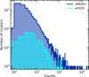 |
Fig. 13 Counts distribution of the confirmed eRASS1 and eFEDS clusters within R500 in the reference band 0.2–2.3 keV (Liu et al. 2022). The majority, 10 178, of the eRASS1 sample (83%), have less than 100 counts within R500. A small fraction, 157 clusters and groups (1%), has over 1000 counts. |
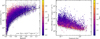 |
Fig. 14 Soft band luminosity distribution of the eRASS1 clusters with redshift shown on the left panel. We only show the luminosities with significant detection at a >2σ confidence for demonstration purposes. The flux value of 4 × 10⁻¹⁴ erg s−1 cm−2 is overplotted as the dashed line. We do not use a flux limit to select clusters; the flux limit is plotted here as a reference. On the right panel, flux within 300 kpc is displayed as a function of exposure time. We only present the significant flux detections with detection confidence >2 σ; the upper limits are excluded from the figure. The color bar indicates zbest. The figure demonstrates that the detection of sources depends on the survey’s depth. |
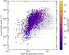 |
Fig. 15 Soft X-ray luminosity in the 0.2–2.3 keV band and temperature relation for a subsample of clusters. The color bar indicates each measurement’s counts within R500. We only show a subselection of 2443 temperature measurements with >35 counts in the sample. |
5.3 Gas mass and total mass measurements
This section describes our method for measuring the integrated properties, including Mgas and M500. To compute the gas mass of a cluster from the electron density profile, we use the enclosed ICM mass within a given aperture obtained by integrating the best-fit density model,
 (4)
(4)
where we assume a metallicity of 0.3Asun of the ICM and a mean molecular weight µe of 1.18. The mass proxy YX is defined as the product of the gas mass and the ICM temperature, YX = Mgas × kT.
Shown in Fig. 16 is the mass distribution of the primary eRASS1 cluster sample, where the mass M500 is estimated by our cosmology pipeline (Ghiradini et al. 2024) after calibrating the count-rate scaling relation with the measured weak lens-ing shear data. These measurements are described in detail in Ghiradini et al. (2024); here, we summarize the process in the cosmology pipeline. In short, we build the probability density function (PDF) of mass as a function of our observed count rate and redshift;
 (5)
(5)
where P(I∣CR, z, 𝓗i) is the selection function calculated at the sky position at each sky position Hi, the uncertainty on count rate and redshift are propagated through  and
and  . The employed scaling relation between count-rate and mass and the mass function is modeled with the P(CR∣ M, z) and P(M, z) terms in the equation. We note that the term
  is not computed since it is just a mass-independent normalization factor. We compute the median and uncertainty on this PDF for 1000 MCMC steps of the cosmology run in the ΛCDM modeling, selecting these points randomly among the final 1000 steps with a thinning factor of 10, namely, among the best 12 000 (Nsteps × Nwalkers)· The total mass (Mtot) and the gas mass fraction (ƒgas = Mgas /Mtot) of each cluster within R500 is calculated using the eROSITA cosmology given in Ghiradini et al. (2024) assuming the best-fit scaling relations between count-rate and weak lensing shear measurements.
We test the aforementioned method, inferring mass within an overdensity radius, R500, from the scaling laws between count rate and mass on the mock observations generated for the cosmology pipeline to verify that the output masses are accurate and bias-free. We find the sum of all the PDFs follows the distribution of the true masses at any redshift bin on an ensemble level. The PDFs of the mass distribution of individual clusters are publicly available in the catalog. However, the median or mean mass values of the low-mass clusters (M500< ∼ 1014 Msun) are biased high, and the median mass of high-mass clusters (M500 >∼ 7 × 10¹⁴ Msun) are biased low. This statistical issue occurs when a mass function and selection are applied to the sample, driving the masses from the count-rate versus mass scaling relations. To correct this bias, we force the mass distribution for each cluster to follow the predicted mass distribution given the cluster-specific count rate and redshift measured. This ensures that recovered mass distribution follows the expected from our modeling. It is important to note that in the cosmology pipeline, cluster masses are marginalized over a probability density function on a sample level; therefore, this observed bias does not affect the cosmology results reported in Ghiradini et al. (2024). We only report the mass estimates where our selection function is reliable.
The masses of the clusters in the primary sample lie in the range of 5 × 10¹² Msun to 10 × 1015 Msun. The median mass of the primary sample within R500 is 1.8 × 10¹⁴ Msun. The 867 high mass clusters with M500 > 5 × 10¹⁴ constitute about 7.1% of the sample. The majority of the sample (71.6%) lies in the intermediate mass regime between 1 × 10¹⁴ Msun < M500 < 5 × 10¹⁴ Msun. The most massive cluster in our sample is 1eRASS 150407.6024816 (ACT-CL J1504.1-0248, PSZ2 G355.07+46.20) with an estimated mass of  Msun an extent likelihood of 479.6 at the redshift of 0.21. This cluster is followed by two clusters with similar mass measurements 1eRASS J102350.1-271526 (PSZ2 G266.83+25.08, SPT ECS J1023-2715) and 1eRASS J134730.8-114510 RXCJ J1347.5-1144, PSZ2 G324.04+48.79) with masses
  Msun at a redshift 0.2 and
  Msun at a redshift 0.45, respectively.
Owing to the superb sensitivity of eROSITA in the soft X-ray band, we find a large number of galaxy groups in our catalog. Although there is no clear dividing line between clusters and groups in the literature, if we classify the latter as haloes with masses M500 < 1014 Msun, we find that about 21.3% of the sample (2610 confirmed sources) lies in the galaxy group regime. The lowest mass group in the sample has a total mass of 5 × 10¹² Msun; the groups detected in eRASS1 represent the largest and cleanest sample to date and will extend our understanding of ICM thermal dynamical properties and AGN feedback to the low-mass regime (Bahar et al. 2024).
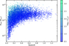 |
Fig. 16 Right panel displays the mass-redshift relation of the eRASS1 cluster sample. M500 is estimated using the scaling relations between count-rate and shear profiles consistent with eROSITA cosmology (Ghiradini et al. 2024). |
5.4 Comparisons of X-ray properties with eFEDS and Chandra
The eFEDS observations, approximately ten times deeper than eRASS1, allow us to test and compare our eRASS1 results with our previous published work. Since eFEDS, we have updated the X-ray data processing software (see Merloni et al. 2024, for details). Additionally, our strategy for cluster analysis has changed with the addition of MBProj2D to the analysis pipeline. 63 of 477 eFEDS clusters have counterparts in eRASS1 (see Sect. 4). Among them, 62 have consistent redshifts within Δz < 0 05, allowing for a direct comparison of the measured X-ray observables. One cluster has an inconsistent redshift as another cluster is detected in projection, leading to different redshift measurements between two different identification methods (see Kluge et al. 2024, for further details). We compare in Fig. 17 the luminosities of these 62 clusters as reported in Liu et al. (2022) and measured in this work, within the same radius of 300 kpc and using the same energy band 0.5–2.0 keV.
Although the methods used in the two works differ from each other, and the data have very different depths, the best-fit of the relation with a slope of 1.01 ± 0.1 indicates that there is no significant offset between eFEDS and eRASS1 in Fig. 17, despite the eRASS1 measurements having relatively large error bars due to the shallower data. A few clusters in the low LX regime have higher luminosities in the eRASS1 catalog than those reported in the eFEDS catalog. In these cases, likely, the source counts are mildly boosted by a nearby AGN in the shallower eRASS1 data (see Clerc et al. 2024, for more information). These AGN are removed from the analysis when measuring the eFEDS luminosities. In eRASS1, due to its shallower depth, they are not detected, their emission contributing to overall cluster eRASS1 luminosity or the Eddington bias.
Deep Chandra archival observations of the previously known eRASS1 clusters, in principle, provide essential tests for the accuracy of our flux determination method and calibration differences (Liu et al. 2023). To understand the (in)consistency in the calibrations between different instruments, comparing the luminosities obtained by eROSITA with those produced using a different X-ray telescope is also helpful. A sound sample consists of the SPT-selected clusters observed by Chandra, which are massive, luminous, and relatively distant. We tookthe sample of 83 clusters analyzed by Sanders et al. (2018) and fit both the Chandra and eROSITA data using MBProj2D, using the same spatial region and point source mask, density parametrization, redshift, cosmology, and Galactic absorption.
In detail, we took the input Chandra images and background in ten bands, input masks, cluster centers, and point source positions from Sanders et al. (2018), binning the images with 2″ pixels. Due to eROSITA’s PSF, we enlarged the point sources excluded in the masks to a minimum of 0′.35 radius and excluded the data beyond a radius of 5 Mpc from the cluster center. These data were fitted with MBProj2D, assuming the density model in Eq. (3), with an isothermal temperature with a flat prior in log space and a metallicity of 0.3Asum. As background models, we took the blank sky fields observation images, smoothed by a Gaussian with σ = 10 pixels, and allowed their overall normalizations to vary freely in the analysis.
For eROSITA, we construct images and exposure maps between 0.2 and 2.3 keV using data from the deeper eRASS:4 survey to obtain better statistics, process with the 020 version of the eSASS pipeline (Merloni et al. 2024), using Telescope Modules (TMs) 1, 2, 3, 4, and 6. The data are filtered using the eSASS tool evtool7 using the option “gti=FLAREGTI” to remove periods containing flares. Section 5.1 describes the rest of the analysis steps. Although this is a newer processing version than the primary dataset presented for eRASS1, the minor differences are insignificant for this analysis. We apply the same mask used for consistency in the Chandra data. These data are fit with MBProj2D, assuming the same model as the Chandra data. However, to avoid issues due to temperature bias, that is, different temperature assumptions might change the luminosity measurements, we fit only the surface brightness in a single energy band (0.2–2.3 keV band). This approach does not allow temperature determination of ICM. We, therefore, assume a log-normal prior on the Chandra temperature posterior probability distribution when measuring the luminosity. The background is assumed to be flat over the fitted region.
Figure 18 shows a comparison between the luminosities in the 0.5–2.0 keV rest frame band obtained by eROSITA and Chandra, for a 600 kpc aperture in the clusters. Overall, the eROSITA and Chandra luminosities scale together. However, the eROSITA luminosities are, on average, around 15% lower than the Chandra ones. We also made a more detailed analysis by doing a joint fit of the Chandra and eROSITA data, allowing the overall cluster luminosity to vary between the telescopes. In this analysis, both data sets are fitted by the same density profile and temperature. In addition, we modeled the point sources near the cluster center in the eROSITA data rather than masking them. This analysis shows fluxes around 15% lower for eROSITA compared to Chandra, consistent with the above analysis. In addition, no evidence for any flux-dependent differences is seen. Some fraction of this comes from the threshold issue, which causes some events to be lost in the processing (Merloni et al. 2024, and K. Dennerl, priv. comm.) although this effect is minor. We will investigate whether calibration differences such as effective area and vignetting could contribute to the remaining difference in the future. In-depth comparisons of cross-calibration between eROSITA and Chandra, XMM-Newton measured temperatures are performed in Migkas et al. (2024). We note that the discrepancy in the flux does not affect the cosmology results presented in Ghiradini et al. (2024) as the scaling relations are internally calibrated for all clusters. However, it should be accounted for in the systematic uncertainties in all other applications.
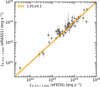 |
Fig. 17 Comparison of the luminosities of the 62 matched clusters detected in eRASS1 and eFEDS. The luminosities are measured within the same radius of 300 kpc and the same energy band of 0.5–2.0 keV. The best-fit line with slope 1.01 ± 0.1 is overplotted in the orange-shaded region. The overall agreement between eFEDS and eRASS1 results is seen regardless of the depth difference between the two surveys. |
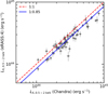 |
Fig. 18 Chandra and eROSITA luminosities of a sample of SPT-selected galaxy clusters. Luminosities are calculated in the 0.5–2.0 keV rest-frame band within a projected radius of 600 kpc. In this plot, only those clusters with an uncertainty of less than 10% from Chandra and 20% from eROSITA are shown (66 out of83). The median ratio between the values suggests that the eROSITA luminosities are lower than the Chandra ones by around 15%. |
6 Population properties of the eRASS1 clusters
In the previous sections, we provided the X-ray properties of the clusters and groups in the eRASS1 sample. This section will compare the population with previous cluster surveys performed in the X-ray band. The completeness and purity of the eRASS1 sample should be accounted for to make meaningful and unbiased comparisons with the literature. Our selection function is constructed based solely on the X-ray detection properties. It cannot replicate the Pcont measurements we apply to the sample due to the lack of richness information in the eROSITA’s digital sky (Seppi et al. 2022). Accordingly, for population studies, we use only a subsample of 6756 clusters selected with the 𝓛ext> 6 threshold, where we are confident about the selection process. The results in this section are provided for this subsample after correcting for the completeness and purity of the sample.
6.1 log N -log S
The observed cluster number counts (N) above a certain flux limit (S), defined as logN-logS or dN/dS, is used to characterize and compare flux-limited cluster surveys (e.g., Rosati et al. 1995; Reiprich & Böhringer 2002). In Fig. 19, we present the log N-log S for the eRASS1 clusters in the primary catalog in the eROSITA reference band 0.2–2.3 keV, after accounting for completeness at each flux limit (Seppi et al. 2022). We base our calculations on the flux measurements within R500, given in the catalog’s FX [R500] column.
The log N–log S distribution of the eRASS1 sample covers more than four orders of magnitude in flux. Higher sensitivity combined with regions with deep exposure in the survey allows constraining the faint end of the distribution down the flux limits of ∼5 × 10⁻¹⁵ erg s−1 cm−2. We have significant constraints in the brightest end of log N–log S. We measure the slope to be −1.2 at high fluxes, while the slope turns shallower in the low flux end (∼10−14 erg s−1 cm−2) where the samples reach high completeness.
We first compare our eRASS1 measurements with the eFEDS log N-log S measurements in the 0.5–2.0 keV band reported in Liu et al. (2022). To convert eFEDS flux measurements to our default 0.2–2.3 keV band, we use the average conversion factor of 1.32. In general, the results of eRASS1 are consistent with eFEDS. The X-ray-selected galaxy clusters in the REFLEX II survey in the southern sky (Böhringer et al. 2017a) and NORAS II in the northern (Böhringer et al. 2017b) extragalactic sky can constrain the bright end of the log N-log S curve. Both surveys have slightly steeper slopes (−1.36 ± 0.07 and −1.4) compared to the eRASS1. The log N-log S distribution is slightly under-predicted in both ROSAT surveys compared to the eRASS1 measurements at the bright end of the log N-log S distribution. However, the discrepancy is only at the 1-2σ level.
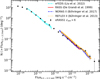 |
Fig. 19 Cumulative cluster number counts as a function of X-ray flux within R500 (log N-log S) in the 0.2–2.3 keV band for the eRASS1 cluster sample. A selection of 𝓛ext> 6 is applied to remove contaminants. Completeness is corrected based on the results of Seppi et al. (2022). Also plotted are the eFEDS result (Liu et al. 2022) and the results from REFLEX II and NORAS II cluster samples based on the ROSAT All-Sky Survey (Böhringer et al. 2013, 2017b). |
6.2 The X-ray luminosity function
Early structure formation models predict a significant increase in the number density of clusters and their evolution per unit volume (Kaiser 1986). This prediction allowed the cluster luminosity and mass functions to be used as tools for constraining cosmology. The cluster X-ray luminosity function (XLF) is also used to study the large-scale structure for cosmological studies in the literature. It is studied in depth for decades in X-ray surveys (see, e.g., Rosati et al. 1998; Vikhlinin et al. 1998; De Grandi et al. 1999; Mullis et al. 2004; Koens et al. 2013; Pacaud et al. 2016; Böhringer et al. 2014; Liu et al. 2022). For instance, substantial negative evolution in the luminosity function is reported in the Einstein X-ray observatory-based cluster samples (e.g. Henry et al. 1992). Although we do not use the XLF as a tool for cosmology, we derive the XLF of eRASS1 clusters and compare it with the published catalogs in this section.
The XLF of a galaxy cluster sample can be computed by counting the number of clusters per effective survey volume in different luminosity bins. This is also called the differential XLF and can be written as;
![${{{\rm{d}}N} \over {{\rm{d}}L}}\left( {\left\langle {{L_i}} \right\rangle } \right) = {1 \over {\Delta {L_i}}}\sum\limits_j {{{1 - P{{{\mathop{\rm cont}\nolimits} }_j}} \over {{V_{{\rm{eff }}}}\left[ {{L_j},{F_{\lim }},A} \right]/P\det \left( {{L_j},{z_j}} \right)}}} ,$](/articles/aa/full_html/2024/05/aa48264-23/aa48264-23-eq22.png) (6)
(6)
where 〈Li〉 and ΔLi are the center luminosity (we use Lx within R500 in 0.2–2.3 keV) and the width of the ith luminosity bin, L/ is the luminosity of the jth cluster in the ith bin. Pdet(Lj, zj) is the detection probability of a cluster with luminosity Lj at red-shift zj, obtained from the selection function. Veff,j[Lj, Flim, A] is the survey-effective volume corresponding to cluster j, as a function of its luminosity Lj, and the flux limit and sky coverage of the survey. To be able to compute Veff, we set a flux limit of 5 × 10⁻¹⁴ erg s−2 cm−2, and the corresponding survey area is 13 116 deg2. The survey depth inhomogeneity is accounted for in the computation of the selection function, where Pdet is given as a sky-average value. The 𝓛ext> 6 sample has < 5% contamination and the stable selection function; therefore, we only compare this sample with the literature.
For the full eRASS1 cluster sample, we divide the luminosity range [5 × 1041 −2 × 1045] erg s−1 into 18 bins with equal logarithmic width. Each bin contains at least 10 clusters. The uncertainty in dN/dL is computed by randomly varying the luminosity for each cluster 1000 times over its statistical uncertainty. This error is then added in quadrature with the Poisson error for the number of clusters in each bin following the approach reported in Liu et al. (2022). The XLF of the primary eRASS1 sample is shown in the left panel of Fig. 20. We compare our results with a survey based on pointed deep ROSAT PSPC observations of the ROSAT All-Sky Survey selected clusters, that is, the Wide Angle ROSAT Pointed Survey (WARPS; Scharf et al. 1997). WARPS covers a similar luminosity and redshift range to eRASS1. Broad agreement between eRASS1 and WARPS XLF (Koens et al. 2013) can be seen in the left panel of Fig. 20. The XLF measured from the two samples in the XXL Survey, containing 365 and 100 clusters, is also consistent with our measurements at the 2σ level. We also show the overall agreement between our results and the COSMOS survey in the redshift range of 0 < z < 0.6 (Finoguenov et al. 2007) and the SPectro-scopic IDentification of eROSITA Sources (SPIDERS) survey in the range 0.3 < z < 0.6 (Clerc et al. 2020). The XLF for the SPIDERS and COSMOS surveys are adopted from Clerc & Finoguenov (2023). We also compare our results with the eFEDS clusters sample presented in Liu et al. (2022). We find that in the low-L500 regime, the XLF in the eFEDS sample is overestimated and underestimated compared to the eRASS1 sample. This difference could be due to the differences in the selection function (studied in detail in Clerc et al. 2024) or the high contamination level (~20%) in the eFEDS sample.
We also investigate the evolution of the XLF by dividing the sample into three redshift bins, 0.003 < zbest < 0.3, 0.3 < zbest < 0.6, and zbest > 0.6. The results are shown in the right panel of Fig. 20. We find that The XLFs in the three redshift bins are consistent with each other within 2σ, indicating no significant evolution in cluster XLF, in agreement with the results of eFEDS (Liu et al. 2022) and other literature (see, e.g., Koens et al. 2013; Clerc & Finoguenov 2023).
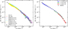 |
Fig. 20 X-ray luminosity function of the eRASS1 cluster sample. Left panel: results for the full sample. Literature results are plotted as the shaded area for comparison: COSMOS (Finoguenov et al. 2007), WARPS (Koens et al. 2013), XXL-100 (Pacaud et al. 2016), XXL-C1 (Adami et al. 2018), SPIDERS (Clerc et al. 2020) surveys. Right panel: results in three redshift bins. No significant XLF evolution is detected in eRASS1 clusters. |
7 Conclusions and summary
We here present the catalog of clusters of galaxies in the Western Galactic hemisphere detected by the first eROSITA All-Sky Survey in the soft energy band (0.2–2.3 keV).
The eRASS1 sample, with 12 247 confirmed galaxy clusters selected in the effective survey area of 13 116 deg2, represents the largest statistically well-defined sample of galaxy clusters and groups based on the ICM selection to date.
The primary cluster catalog is constructed based on a low extent likelihood criterion (𝓛ext> 3) to maximize completeness and the detection rate of compact high-z clusters and groups (Merloni et al. 2024). The estimated purity of this sample is 86%, while the approximate flux limit is 4 × 10⁻¹⁴ ergs cm−2 s−1. The sample comprises clusters and groups in a wide redshift range from 0.003 to 1.32 with a sample median zbest,med = 0.31. The masses of clusters in the catalog span a large interval from 1012 Msun to 4 × 10¹⁵ Msun, with a median value of 3.2 × 10¹⁴ Msun. We introduce a new cleaning strategy, the mixture model method, based on the X-ray and optical detection properties, which can increase the purity level to 95% in the primary cluster catalog. When cross-matched with the other cluster catalogs compiled from X-ray, SZ, and optical surveys, we find that the eRASS1 primary cluster catalog contains 8361 unique detections (68% of the sample), namely, newly discovered clusters or groups.
Cosmological studies benefit from the use of relatively pure galaxy cluster samples. An efficient way of reaching any desired purity levels is to select a sample with a strict X-ray extent selection. Cleaning the primary cluster sample with 𝓛ext cuts ensures that the projection issues in the optical data through richness do not impact the final sample. With a stricter X-ray selection on the primary sample, for instance, taking 𝓛ext > 10 in the same footprint, cluster samples with 98% purity can be obtained at the cost of reducing the number of clusters by around a factor of 3. On the other hand, increasing the 𝓛ext cut to > 6 in the 12 791 deg2 LS DR10-south footprint for the cosmology sample gives purity levels on the order of 95% in a sample of 5259 clusters.
To provide precise X-ray properties of the sample, we reprocess the eRASS1 X-ray data for the clusters in the sample. The improvements include a careful treatment of the X-ray background with advanced modeling of the cluster emission, K-factor, and galactic absorption corrections. In the primary catalog, we provide the resulting X-ray properties of each cluster with a redshift measurement. These properties, including (but not limited to) counts, count-rate, luminosity, flux, ICM temperature, gas mass, total mass, gas mass fraction, and mass proxy YX, are provided in the primary catalog. For the cosmology sample, we provide the count rate, the primary X-ray mass proxy used in cosmological analyses, with the same advanced X-ray analysis applied to the primary sample to reduce the scatter between the mass proxy and cluster mass.
We find consistent results when we compare the reported observed properties, such as the band averaged luminosity, of 62 clusters commonly detected in eFEDS and eRASS1 in the overlapping footprint. However, in a sample of massive clusters observed with Chandra, we find that the luminosity measured by eROSITA in this work is, on average, ~15% lower than the Chandra measurement. This calibration difference is an active area of investigation and will be addressed in future work.
The eRASS1 cluster sample properties, such as log N-log S and the luminosity function, offer an opportunity to compare the cluster population with previous X-ray cluster catalogs in the literature. The catalog’s selection function, purity, and completeness are considered when studying both log N-log S and the XLF of the sample. While we extend the measurements of log N–log S and XLF to five orders of magnitude, we find good agreement between the log N–log S and XLF with previous X-ray surveys based on ROSAT and XMM-Newton data, including the XXL, REFLEX II, NORAS II, and WARPS surveys in the respective flux and luminosity ranges covered by these surveys. We find no significant evolution of the cluster luminosity function in the redshift range of 0.003 and 1.3, consistent with our previous eFEDS results.
The eRASS1 primary cluster and group catalogs provide the largest ICM-based sample of galaxy groups and clusters of galaxies with a well-defined selection function and high purity. This sample will be employed in various astrophysical, large-scale structure formation, and cosmological studies and will result in novel results when the selection effects are adequately accounted for. We confirm the excellent performance of eROSITA for clusters and groups science and show that pre-launch predictions for detecting 100 000 clusters and groups will be met when the final survey depth (eRASS:8) is reached at the end of the survey program.
Acknowledgements
The authors thank the referee for helpful and constructive comments on the draft. The authors thank Johannes Buchner and J. Michael Burgess for insightful discussions on the statistical methods of mass calculations. This work is based on data from eROSITA, the soft X-ray instrument aboard SRG, a joint Russian-German science mission supported by the Russian Space Agency (Roskosmos), in the interests of the Russian Academy of Sciences represented by its Space Research Institute (IKI), and the Deutsches Zentrum für Luft und Raumfahrt (DLR). The SRG spacecraft was built by Lavochkin Association (NPOL) and its subcontractors and is operated by NPOL with support from the Max Planck Institute for Extraterrestrial Physics (MPE). The development and construction of the eROSITA X-ray instrument were led by MPE, with contributions from the Dr. Karl Remeis Observatory Bamberg & ECAP (FAU Erlangen-Nuernberg), the University of Hamburg Observatory, the Leibniz Institute for Astrophysics Potsdam (AIP), and the Institute for Astronomy and Astrophysics of the University of Tübingen, with the support of DLR and the Max Planck Society. The Argelander Institute for Astronomy of the University of Bonn and the Ludwig Maximilians Universität Munich also participated in the science preparation for eROSITA. The eROSITA data shown here were processed using the eSASS/NRTA software system developed by the German eROSITA consortium. E. Bulbul, A. Liu, V. Ghirardini, C. Garrel, S. Zelmer, and X. Zhang acknowledge financial support from the European Research Council (ERC) Consolidator Grant under the European Union’s Horizon 2020 research and innovation program (grant agreement CoG DarkQuest No. 101002585). N. Clerc was financially supported by CNES. A. Veronica acknowledges funding by the Deutsche Forschungsgemeinschaft (DFG, German Research Foundation) – 450861021. T. Schrabback and F. Kleinebreil acknowledge support from the German Federal Ministry for Economic Affairs and Energy (BMWi) provided through DLR under projects 50OR2002, 50OR2106, and 50OR2302, as well as the support provided by the Deutsche Forschungsgemeinschaft (DFG, German Research Foundation) under grant 415537506. The Legacy Surveys consist of three individual and complementary projects: the Dark Energy Camera Legacy Survey (DECaLS; Proposal ID #2014B-0404; PIs: David Schlegel and Arjun Dey), the Beijing-Arizona Sky Survey (BASS; NOAO Prop. ID #2015A-0801; PIs: Zhou Xu and Xiaohui Fan), and the Mayall z-band Legacy Survey (MzLS; Prop. ID #2016A-0453; PI: Arjun Dey). DECaLS, BASS and MzLS together include data obtained, respectively, at the Blanco telescope, Cerro Tololo Inter-American Observatory, NSF’s NOIRLab; the Bok telescope, Steward Observatory, University of Arizona; and the Mayall telescope, Kitt Peak National Observatory, NOIRLab. Pipeline processing and analyses of the data were supported by NOIRLab and the Lawrence Berkeley National Laboratory (LBNL). The Legacy Surveys project is honored to be permitted to conduct astronomical research on Iolkam Du'ag (Kitt Peak), a mountain with particular significance to the Tohono O’odham Nation. This work made use of SciPy (Jones et al. 2001), matplotlib, a Python library for publication-quality graphics (Hunter 2007), Astropy, a community-developed core Python package for Astronomy (Astropy Collaboration 2013), NumPy (Van Der Walt et al. 2011).
Appendix A MBProj2D
MBProj2D8, a Multi-Band Projector in 2D, is a software code for fitting the X-ray images of clusters to determine their physical properties. By fitting simultaneously in multiple energy bands, the software is sensitive to the temperature and metallicity of the gas, in addition to the density. As the number of energy bands increases, the accuracy for temperature measurements should tend toward that of the spectral fitting. The code is forward-fitting, where a physical model of the cluster is used to produce model images. These images are then compared to the observed X-ray data to obtain a Poisson likelihood. MCMC, using this likelihood and incorporating priors, can then be used to obtain posterior probability distributions of the model parameters. The MCMC chains are post-processed to produce profiles of physical quantities and their uncertainties. MBProj2D builds upon the heritage of its predecessors, MBProj2 (Sanders et al. 2018) and MBProj (Sanders et al. 2014), using the same primary method of fitting in multiple energy bands, although much of the code has been rewritten or restructured. The main difference is that it now models clusters in two dimensions rather than using radial profiles. This extension into 2D has the advantage that multiple possibly overlapping clusters can be simultaneously fitted by the code, which is necessary for a good description of eROSITA data. Point sources can also be included in the model rather than masked out of the images, essential if they are bright or near the cluster center. Although two dimensions more easily allow the incorporation of the properties of the telescope and detector, such as the PSF or the background, a disadvantage is that it is more computationally expensive to model images rather than profiles. The new version also removes several restrictions, including the cluster model being able to extend beyond the region examined.
The input data are statistically independent X-ray count images of the cluster in multiple energy bands. A restriction removed in this version is that the data can come from different observations or X-ray telescopes, even if the pixel sizes differ. As for the previous versions of the code, these bands should be chosen to cover the energy range of the instrument, taking into account the variation in the effective area as a function of the area and providing sensitivity to the gas temperature. In addition, exposure maps are required in each band, where the value at a position is the exposure time in that band appropriate for a provided response matrix and ancillary response matrix. Currently, MBProj2D assumes that the same response matrix is valid over the field, which is correct for eROSITA —however, the exposure map accounts for ancillary response variations such as vignetting. The user can also provide a 2D PSF model for the telescope, which is assumed to be constant across the field.
MBProj2D is a flexible framework written in Python9 for describing a cluster field, fitting this model, obtaining uncertainties on it using MCMC, and then turning the acquired chains into physical profiles or model images. The user writes a Python script to load the data, describe the model, parameters, and priors, and then conduct the analysis. A block diagram of the various components is shown in Fig. A.1. The code is highly extensible, allowing users to add multiple source and background components, parametrizations of radial properties, hydrostatic mass models, or Bayesian priors. Some more computationally expensive routines are written in C++, including code for projecting the one-dimensional cluster profiles onto the sky and calculating model likelihoods.
MBProj2D can either fit clusters in which the temperature, gas density, and metallicity profiles are described using arbitrary parametrizations, or it can fit clusters under the assumption of hydrostatic equilibrium, where the user provides parametrized dark matter or total mass profiles and gas density and metallicity profiles. In the hydrostatic case, the equation of hydrostatic equilibrium is used to calculate a pressure profile, and its temperature can be computed using gas density.
In detail, the parametrized cluster profiles are converted into 3D emissivity profiles for each energy band, using Xspec (Arnaud 1996) with the APEC model (Smith et al. 2001) to convert between temperature, density, metallicity to emissivity, given absorption by a fixed Galactic HI column, calculated using TBABS (Wilms et al. 2000). The profiles are projected onto the sky to make a rate image, given a parametrized cluster central position, out to some fixed physical cluster radius. Although not used in this paper, the code can also include ellipticity on the sky in the model. Added to the image are any point sources, where a power-law spectral index, normalization, and position parameters are used to describe the source. The total model image is convolved with the instrument PSF using a Fast Fourier Transform to produce a smoothed model image. This rate image is multiplied by the exposure maps to make a count image. Background components are added to the source image to make a total model counts image. As an observed image can include contaminating point sources or detector features, the user provides a mask image that selects the valid regions, for example. Given the combined model count image, the mask image, and the observed count image, a Poisson likelihood is computed. The likelihoods for each input band and image are combined to give a total Pois-son likelihood. Any Bayesian priors on the model parameters or components are added to this likelihood.
Typically, the user fits the model to the data to find the parameters to start an MCMC analysis. MCMC is used to obtain a chain of parameters, optionally using multiple CPU cores to speed up the analysis, here using the emcee affine invariant ensemble sampler (Foreman-Mackey et al. 2013). This posterior probability distribution of the chain parameters can be examined directly. Alternatively, the chains can be post-processed to create other outputs. These include X-ray images in each band and residual maps and profiles, showing the distribution of the difference between the data and models extracted from the chain. The maps can also be binned using Voronoi tessellation for clarity by adjusting for the local signal-to-noise ratio. The parameters in the chain can be converted into profiles of physically interesting quantities and their uncertainties for each cluster. The median profiles and their range can be calculated for the primary parametrization (gas density and temperature). Many further derived quantities can be calculated, including pressure, entropy, luminosity, flux, X-ray count rates, mean radiative cooling time, gas mass, total hydrostatic mass (if fitting a hydrostatic model), cooling flow mass deposition rate, and YX.
 |
Fig. A.1 Block diagram showing the components of MBProj2D and their relationships. Names that correspond to classes defined in MBProj2D are shown in italics. Solid arrows show direct connections, while weaker connections are dashed. |
References
- Abell, G. O., Corwin, Harold G., J., & Olowin, R. P. 1989, ApJS, 70, 1 [NASA ADS] [CrossRef] [Google Scholar]
- Adami, C., Giles, P., Koulouridis, E., et al. 2018, A&A, 620, A5 [NASA ADS] [CrossRef] [EDP Sciences] [Google Scholar]
- Almeida, A., Anderson, S. F., Argudo-Fernández, M., et al. 2023, ApJS, 267, 44 [NASA ADS] [CrossRef] [Google Scholar]
- Andernach, H. 1991, in ASP Conf. Ser., 15, Large-scale Structures and Peculiar Motions in the Universe, eds. D. W. Latham, & L. A. N. da Costa, 279 [Google Scholar]
- Arnaud, K. A. 1996, in ASP Conf. Ser. 101: Astronomical Data Analysis Software and Systems V, eds. G. H. Jacoby, & J. Barnes, 17 [Google Scholar]
- Artis, E., Ghirardini, V., Bulbul, E., et al. 2024, A&A submitted [arXiv:2402.08459] [Google Scholar]
- Asplund, M., Grevesse, N., Sauval, A. J., & Scott, P. 2009, ARA&A, 47, 481 [NASA ADS] [CrossRef] [Google Scholar]
- Astropy Collaboration (Robitaille, T. P., et al.) 2013, A&A, 558, A33 [NASA ADS] [CrossRef] [EDP Sciences] [Google Scholar]
- Bahar, Y. E., Bulbul, E., Clerc, N., et al. 2022, A&A, 661, A7 [NASA ADS] [CrossRef] [EDP Sciences] [Google Scholar]
- Bahar, Y. E., Bulbul, E., Ghirardini, V., et al. 2024, A&A, submitted [arXiv:2401.17276] [Google Scholar]
- Balogh, M. L., van der Burg, R. F. J., Muzzin, A., et al. 2021, MNRAS, 500, 358 [Google Scholar]
- Becker, W., Hurley-Walker, N., Weinberger, C., et al. 2021, A&A, 648, A30 [NASA ADS] [CrossRef] [EDP Sciences] [Google Scholar]
- Bleem, L. E., Stalder, B., de Haan, T., et al. 2015, ApJS, 216, 27 [Google Scholar]
- Bleem, L. E., Bocquet, S., Stalder, B., et al. 2020, ApJS, 247, 25 [Google Scholar]
- Bocquet, S., Dietrich, J. P., Schrabback, T., et al. 2019, ApJ, 878, 55 [Google Scholar]
- Boese, F. G. 2000, A&AS, 141, 507 [NASA ADS] [CrossRef] [EDP Sciences] [Google Scholar]
- Böhringer, H., Voges, W., Huchra, J. P., et al. 2000, ApJS, 129, 435 [Google Scholar]
- Böhringer, H., Schuecker, P., Guzzo, L., et al. 2004, A&A, 425, 367 [NASA ADS] [CrossRef] [EDP Sciences] [Google Scholar]
- Böhringer, H., Chon, G., Collins, C. A., et al. 2013, A&A, 555, A30 [Google Scholar]
- Böhringer, H., Chon, G., & Collins, C. A. 2014, A&A, 570, A31 [NASA ADS] [CrossRef] [EDP Sciences] [Google Scholar]
- Böhringer, H., Chon, G., & Fukugita, M. 2017a, A&A, 608, A65 [NASA ADS] [CrossRef] [EDP Sciences] [Google Scholar]
- Böhringer, H., Chon, G., Retzlaff, J., et al. 2017b, AJ, 153, 220 [Google Scholar]
- Brunner, H., Liu, T., Lamer, G., et al. 2022, A&A, 661, A1 [NASA ADS] [CrossRef] [EDP Sciences] [Google Scholar]
- Bulbul, G. E., Hasler, N., Bonamente, M., & Joy, M. 2010, ApJ, 720, 1038 [NASA ADS] [CrossRef] [Google Scholar]
- Bulbul, E., Markevitch, M., Foster, A., et al. 2014, ApJ, 789, 13 [NASA ADS] [CrossRef] [Google Scholar]
- Bulbul, E., Chiu, I. N., Mohr, J. J., et al. 2019, ApJ, 871, 50 [Google Scholar]
- Bulbul, E., Liu, A., Pasini, T., et al. 2022, A&A, 661, A10 [NASA ADS] [CrossRef] [EDP Sciences] [Google Scholar]
- Burenin, R. A., Vikhlinin, A., Hornstrup, A., et al. 2007, ApJS, 172, 561 [Google Scholar]
- Chiu, I. N., Ghirardini, V., Liu, A., et al. 2022, A&A, 661, A11 [NASA ADS] [CrossRef] [EDP Sciences] [Google Scholar]
- Chuang, C.-H., Yepes, G., Kitaura, F.-S., et al. 2019, MNRAS, 487, 48 [NASA ADS] [CrossRef] [Google Scholar]
- Clerc, N., & Finoguenov, A. 2023, in Handbook of X-ray and Gamma-ray Astrophysics, eds. C. Bambi & A. Santangelo, 123 [Google Scholar]
- Clerc, N., Merloni, A., Zhang, Y. Y., et al. 2016, MNRAS, 463, 4490 [NASA ADS] [CrossRef] [Google Scholar]
- Clerc, N., Kirkpatrick, C. C., Finoguenov, A., et al. 2020, MNRAS, 497, 3976 [NASA ADS] [CrossRef] [Google Scholar]
- Clerc, N., Comparat, J., Seppi, R., et al. 2024, A&A, submitted [arXiv:2402.08457] [Google Scholar]
- Colless, M., Dalton, G., Maddox, S., et al. 2001, MNRAS, 328, 1039 [Google Scholar]
- Comparat, J., Merloni, A., Salvato, M., et al. 2019, MNRAS, 487, 2005 [Google Scholar]
- Comparat, J., Eckert, D., Finoguenov, A., et al. 2020, Open J. Astrophys., 3, 13 [Google Scholar]
- Costanzi, M., Rozo, E., Rykoff, E. S., et al. 2019, MNRAS, 482, 490 [CrossRef] [Google Scholar]
- Cruddace, R., Voges, W., Böhringer, H., et al. 2002, ApJS, 140, 239 [NASA ADS] [CrossRef] [Google Scholar]
- Dauser, T., Falkner, S., Lorenz, M., et al. 2019, A&A, 630, A66 [NASA ADS] [CrossRef] [EDP Sciences] [Google Scholar]
- De Grandi, S., Böhringer, H., Guzzo, L., et al. 1999, ApJ, 514, 148 [NASA ADS] [CrossRef] [Google Scholar]
- Dey, A., Schlegel, D. J., Lang, D., et al. 2019, AJ, 157, 168 [Google Scholar]
- Driver, S. P., Bellstedt, S., Robotham, A. S. G., et al. 2022, MNRAS, 513, 439 [NASA ADS] [CrossRef] [Google Scholar]
- Ebeling, H., Edge, A. C., Bohringer, H., et al. 1998, MNRAS, 301, 881 [Google Scholar]
- Ezer, C., Bulbul, E., Nihal Ercan, E., et al. 2017, ApJ, 836, 110 [NASA ADS] [CrossRef] [Google Scholar]
- Finoguenov, A., Guzzo, L., Hasinger, G., et al. 2007, ApJS, 172, 182 [Google Scholar]
- Finoguenov, A., Merloni, A., Comparat, J., et al. 2019, The Messenger, 175, 39 [NASA ADS] [Google Scholar]
- Finoguenov, A., Rykoff, E., Clerc, N., et al. 2020, A&A, 638, A114 [NASA ADS] [CrossRef] [EDP Sciences] [Google Scholar]
- Foreman-Mackey, D., Hogg, D. W., Lang, D., & Goodman, J. 2013, PASP, 125, 306 [Google Scholar]
- Geller, M. J., & Huchra, J. P. 1989, Science, 246, 897 [NASA ADS] [CrossRef] [Google Scholar]
- Ghirardini, V., Eckert, D., Ettori, S., et al. 2019, A&A, 621, A41 [NASA ADS] [CrossRef] [EDP Sciences] [Google Scholar]
- Ghirardini, V., Bulbul, E., Hoang, D. N., et al. 2021, A&A, 647, A4 [EDP Sciences] [Google Scholar]
- Ghirardini, V., Bahar, Y. E., Bulbul, E., et al. 2022, A&A, 661, A12 [NASA ADS] [CrossRef] [EDP Sciences] [Google Scholar]
- Ghiradini, V., Bulbul, E., Artis, E., et al. 2024, A&A, submitted [arXiv:2402.08458] [Google Scholar]
- Giacani, E. B., Dubner, G. M., Green, A. J., Goss, W. M., & Gaensler, B. M. 2000, AJ, 119, 281 [Google Scholar]
- Gonzalez, A. H., Gettings, D. P., Brodwin, M., et al. 2019, ApJS, 240, 33 [NASA ADS] [CrossRef] [Google Scholar]
- Grandis, S., Mohr, J. J., Costanzi, M., et al. 2021, MNRAS, 504, 1253 [NASA ADS] [CrossRef] [Google Scholar]
- Grandis, S., Ghirardini, E., Bocquet, S. et al. 2024, A&A, submitted [arXiv:2402.08455] [Google Scholar]
- Harris, W. E. 2010, arXiv e-prints [arXiv:1012.3224] [Google Scholar]
- Henry, J. P., Gioia, I. M., Maccacaro, T., et al. 1992, ApJ, 386, 408 [NASA ADS] [CrossRef] [Google Scholar]
- HI4PI Collaboration (Ben Bekhti, N., et al.) 2016, A&A, 594, A116 [NASA ADS] [CrossRef] [EDP Sciences] [Google Scholar]
- Hilton, M., Sifón, C., Naess, S., et al. 2021, ApJS, 253, 3 [Google Scholar]
- Hlavacek-Larrondo, J., McDonald, M., Benson, B. A., et al. 2015, ApJ, 805, 35 [NASA ADS] [CrossRef] [Google Scholar]
- Huang, N., Bleem, L. E., Stalder, B., et al. 2020, AJ, 159, 110 [Google Scholar]
- Huang, X., Storfer, C., Gu, A., et al. 2021, ApJ, 909, 27 [NASA ADS] [CrossRef] [Google Scholar]
- Hudson, D. S., Mittal, R., Reiprich, T. H., et al. 2010, A&A, 513, A37 [NASA ADS] [CrossRef] [EDP Sciences] [Google Scholar]
- Hunter, J. D. 2007, Comput. Sci. Eng., 9, 90 [NASA ADS] [CrossRef] [Google Scholar]
- Huterer, D., & Shafer, D. L. 2018, Rep. Progr. Phys., 81, 016901 [CrossRef] [Google Scholar]
- Ider Chitham, J., Comparat, J., Finoguenov, A., et al. 2020, MNRAS, 499, 4768 [NASA ADS] [CrossRef] [Google Scholar]
- Jones, E., Oliphant, T., Peterson, P., et al. 2001, SciPy: Open source scientific tools for Python [Google Scholar]
- Kaastra, J. S. 2017, A&A, 605, A51 [NASA ADS] [CrossRef] [EDP Sciences] [Google Scholar]
- Käfer, F., Finoguenov, A., Eckert, D., et al. 2020, A&A, 634, A8 [Google Scholar]
- Kaiser, N. 1986, MNRAS, 222, 323 [Google Scholar]
- Kirk, B., Hilton, M., Cress, C., et al. 2015, MNRAS, 449, 4010 [NASA ADS] [CrossRef] [Google Scholar]
- Klein, M., Grandis, S., Mohr, J. J., et al. 2019, MNRAS, 488, 739 [Google Scholar]
- Klein, M., Oguri, M., Mohr, J. J., et al. 2022, A&A, 661, A4 [NASA ADS] [CrossRef] [EDP Sciences] [Google Scholar]
- Klein, M., Hernández-Lang, D., Mohr, J. J., Bocquet, S., & Singh, A. 2023, MNRAS, 526, 3757 [NASA ADS] [CrossRef] [Google Scholar]
- Kleinebreil, A., Schrabback, T., Grandis, S., et al. 2024 A&A, submitted [arXiv:2402.08456] [NASA ADS] [CrossRef] [EDP Sciences] [Google Scholar]
- Kluge, M., Comparat, J., Liu, A., et al. 2024, A&A, submitted [arXiv:2402.08453] [Google Scholar]
- Koens, L. A., Maughan, B. J., Jones, L. R., et al. 2013, MNRAS, 435, 3231 [CrossRef] [Google Scholar]
- Kollmeier, J. A., Zasowski, G., Rix, H.-W., et al. 2017, arXiv e-prints [arXiv:1711.03234] [Google Scholar]
- Koulouridis, E., Clerc, N., Sadibekova, T., et al. 2021, A&A, 652, A12 [NASA ADS] [CrossRef] [EDP Sciences] [Google Scholar]
- Krippendorf, S., Baron Perez, N., Bulbul, E., et al. 2024, A&A, 682, A132 [NASA ADS] [CrossRef] [EDP Sciences] [Google Scholar]
- Leahy, D. A., Ranasinghe, S., & Gelowitz, M. 2020, ApJS, 248, 16 [NASA ADS] [CrossRef] [Google Scholar]
- Liu, Q. Z., van Paradijs, J., & van den Heuvel, E. P. J. 2006, A&A, 455, 1165 [NASA ADS] [CrossRef] [EDP Sciences] [Google Scholar]
- Liu, Q. Z., van Paradijs, J., & van den Heuvel, E. P. J. 2007, A&A, 469, 807 [NASA ADS] [CrossRef] [EDP Sciences] [Google Scholar]
- Liu, A., Yu, H., Tozzi, P., & Zhu, Z.-H. 2016, ApJ, 821, 29 [Google Scholar]
- Liu, A., Tozzi, P., Ettori, S., et al. 2020, A&A, 637, A58 [NASA ADS] [CrossRef] [EDP Sciences] [Google Scholar]
- Liu, A., Bulbul, E., Ghirardini, V., et al. 2022, A&A, 661, A2 [NASA ADS] [CrossRef] [EDP Sciences] [Google Scholar]
- Liu, A., Bulbul, E., Ramos-Ceja, M. E., et al. 2023, A&A, 670, A96 [NASA ADS] [CrossRef] [EDP Sciences] [Google Scholar]
- Liu, A., Bulbul, E., Ghirardini, V., et al. 2024, A&A, 683, A130 [NASA ADS] [CrossRef] [EDP Sciences] [Google Scholar]
- Lovisari, L., Ettori, S., Gaspari, M., & Giles, P. A. 2021, Universe, 7, 139 [NASA ADS] [CrossRef] [Google Scholar]
- Malmquist, K. G. 1922, Meddelanden fran Lunds Astronomiska Observatorium Serie I, 100, 1 [Google Scholar]
- Maturi, M., Bellagamba, F., Radovich, M., et al. 2019, MNRAS, 485, 498 [Google Scholar]
- McClintock, T., Varga, T. N., Gruen, D., et al. 2019, MNRAS, 482, 1352 [Google Scholar]
- Mehrtens, N., Romer, A. K., Hilton, M., et al. 2012, MNRAS, 423, 1024 [NASA ADS] [CrossRef] [Google Scholar]
- Merloni, A., Predehl, P., Becker, W., et al. 2012, ArXiv e-prints [arXiv:1209.3114] [Google Scholar]
- Merloni, A., Lamer, G., Liu, T., et al. 2024, A&A, 682, A34 [NASA ADS] [CrossRef] [EDP Sciences] [Google Scholar]
- Mernier, F., Biffi, V., Yamaguchi, H., et al. 2018, Space Sci. Rev., 214, 129 [Google Scholar]
- Migkas, K., Kox, D., Schellenberger, G., et al. 2024, A&A, submitted, [arXiv:2401.17297] [Google Scholar]
- Moresco, M., Amati, L., Amendola, L., et al. 2022, Living Rev. Relativity, 25, 6 [NASA ADS] [CrossRef] [Google Scholar]
- Mullis, C. R., Vikhlinin, A., Henry, J. P., et al. 2004, ApJ, 607, 175 [NASA ADS] [CrossRef] [Google Scholar]
- Myles, J., Gruen, D., Mantz, A. B., et al. 2021, MNRAS, 505, 33 [NASA ADS] [CrossRef] [Google Scholar]
- Oguri, M., Lin, Y.-T., Lin, S.-C., et al. 2018, PASJ, 70, S20 [NASA ADS] [Google Scholar]
- Ota, N., Nguyen-Dang, N. T., Mitsuishi, I., et al. 2023, A&A, 669, A110 [NASA ADS] [CrossRef] [EDP Sciences] [Google Scholar]
- Pacaud, F., Clerc, N., Giles, P. A., et al. 2016, A&A, 592, A2 [NASA ADS] [CrossRef] [EDP Sciences] [Google Scholar]
- Pasini, T., Brüggen, M., Hoang, D. N., et al. 2022, A&A, 661, A13 [NASA ADS] [CrossRef] [EDP Sciences] [Google Scholar]
- Perlmutter, S., Aldering, G., Goldhaber, G., et al. 1999, ApJ, 517, 565 [Google Scholar]
- Pierre, M., Pacaud, F., Adami, C., et al. 2016, A&A, 592, A1 [NASA ADS] [CrossRef] [EDP Sciences] [Google Scholar]
- Piffaretti, R., Arnaud, M., Pratt, G. W., Pointecouteau, E., & Melin, J. B. 2011, A&A, 534, A109 [NASA ADS] [CrossRef] [EDP Sciences] [Google Scholar]
- Pillepich, A., Porciani, C., & Reiprich, T. H. 2012, MNRAS, 422, 44 [Google Scholar]
- Planck Collaboration VII. 2014, A&A, 571, A7 [NASA ADS] [CrossRef] [EDP Sciences] [Google Scholar]
- Planck Collaboration XXVII. 2016, A&A, 594, A27 [NASA ADS] [CrossRef] [EDP Sciences] [Google Scholar]
- Popesso, P., Biviano, A., Bulbul, E., et al. 2024, MNRAS, 527, 895 [Google Scholar]
- Pratt, G. W., Arnaud, M., Biviano, A., et al. 2019, Space Sci. Rev., 215, 25 [Google Scholar]
- Pratt, G. W., Arnaud, M., Maughan, B. J., & Melin, J. B. 2022, A&A, 665, A24 [NASA ADS] [CrossRef] [EDP Sciences] [Google Scholar]
- Predehl, P., Andritschke, R., Arefiev, V., et al. 2021, A&A, 647, A1 [EDP Sciences] [Google Scholar]
- Ramos-Ceja, M. E., Basu, K., Pacaud, F., & Bertoldi, F. 2015, A&A, 583, A111 [NASA ADS] [CrossRef] [EDP Sciences] [Google Scholar]
- Ramos-Ceja, M. E., Oguri, M., Miyazaki, S., et al. 2022, A&A, 661, A14 [NASA ADS] [CrossRef] [EDP Sciences] [Google Scholar]
- Rana, D., More, S., Miyatake, H., et al. 2023, MNRAS, 522, 4181 [NASA ADS] [CrossRef] [Google Scholar]
- Reiprich, T. H., & Böhringer, H. 2002, ApJ, 567, 716 [Google Scholar]
- Reynolds, C. S., Marsh, M. C. D., Russell, H. R., et al. 2020, ApJ, 890, 59 [NASA ADS] [CrossRef] [Google Scholar]
- Riess, A. G., Filippenko, A. V., Challis, P., et al. 1998, AJ, 116, 1009 [Google Scholar]
- Rojas Bolivar, R. A., Wik, D. R., Giacintucci, S., et al. 2021, ApJ, 906, 87 [CrossRef] [Google Scholar]
- Rosati, P., Della Ceca, R., Burg, R., Norman, C., & Giacconi, R. 1995, ApJ, 445, L11 [NASA ADS] [CrossRef] [Google Scholar]
- Rosati, P., Della Ceca, R., Norman, C., & Giacconi, R. 1998, ApJ, 492, L21 [NASA ADS] [CrossRef] [Google Scholar]
- Rossetti, M., Gastaldello, F., Eckert, D., et al. 2017, MNRAS, 468, 1917 [Google Scholar]
- Rykoff, E. S., Rozo, E., Busha, M. T., et al. 2014, ApJ, 785, 104 [Google Scholar]
- Rykoff, E. S., Rozo, E., Hollowood, D., et al. 2016, ApJS, 224, 1 [NASA ADS] [CrossRef] [Google Scholar]
- Sanders, J. 2024, A&A, submitted [Google Scholar]
- Sanders, J. S., Fabian, A. C., Hlavacek-Larrondo, J., et al. 2014, MNRAS, 444, 1497 [NASA ADS] [CrossRef] [Google Scholar]
- Sanders, J. S., Fabian, A. C., Russell, H. R., & Walker, S. A. 2018, MNRAS, 474, 1065 [NASA ADS] [CrossRef] [Google Scholar]
- Sanders, J. S., Dennerl, K., Russell, H. R., et al. 2020, A&A, 633, A42 [EDP Sciences] [Google Scholar]
- Scharf, C. A., Ebeling, H., Perlman, E., Malkan, M., & Wegner, G. 1997, ApJ, 477, 79 [NASA ADS] [CrossRef] [Google Scholar]
- Seppi, R., Comparat, J., Bulbul, E., et al. 2022, A&A, 665, A78 [NASA ADS] [CrossRef] [EDP Sciences] [Google Scholar]
- Seppi, R., Comparat, J., Nandra, K., et al. 2023, A&A, 671, A57 [NASA ADS] [CrossRef] [EDP Sciences] [Google Scholar]
- Seppi, R., Comparat, C., Ghirardini, V., et al. 2024, A&A, submitted [arXiv:2402.08460] [Google Scholar]
- Smith, R. K., Brickhouse, N. S., Liedahl, D. A., & Raymond, J. C. 2001, ApJ, 556, L91 [Google Scholar]
- Sunyaev, R., Arefiev, V., Babyshkin, V., et al. 2021, A&A, 656, A132 [NASA ADS] [CrossRef] [EDP Sciences] [Google Scholar]
- Truemper, J. 1982, Adv. Space Res., 2, 241 [Google Scholar]
- Van Der Walt, S., Colbert, S. C., & Varoquaux, G. 2011, Comput. Sci. Eng., 13, 22 [Google Scholar]
- van Haarlem, M. P., Frenk, C. S., & White, S. D. M. 1997, MNRAS, 287, 817 [CrossRef] [Google Scholar]
- van Weeren, R. J., de Gasperin, F., Akamatsu, H., et al. 2019, Space Sci. Rev., 215, 16 [Google Scholar]
- Vikhlinin, A., McNamara, B. R., Forman, W., et al. 1998, ApJ, 498, L21 [NASA ADS] [CrossRef] [Google Scholar]
- Vikhlinin, A., Kravtsov, A., Forman, W., et al. 2006, ApJ, 640, 691 [Google Scholar]
- Voges, W., Aschenbach, B., Boller, T., et al. 1999, A&A, 349, 389 [NASA ADS] [Google Scholar]
- Wen, Z. L., & Han, J. L. 2018, MNRAS, 481, 4158 [CrossRef] [Google Scholar]
- Willingale, R., Starling, R. L. C., Beardmore, A. P., Tanvir, N. R., & O’Brien, P. T. 2013, MNRAS, 431, 394 [Google Scholar]
- Wilms, J., Allen, A., & McCray, R. 2000, ApJ, 542, 914 [Google Scholar]
- Wilson, G., Muzzin, A., Yee, H. K. C., et al. 2009, ApJ, 698, 1943 [Google Scholar]
- Winkler, P. F., Williams, B. J., Reynolds, S. P., et al. 2014, ApJ, 781, 65 [NASA ADS] [CrossRef] [Google Scholar]
- Xu, W., Ramos-Ceja, M. E., Pacaud, F., Reiprich, T. H., & Erben, T. 2022, A&A, 658, A59 [NASA ADS] [CrossRef] [EDP Sciences] [Google Scholar]
- Zhang, X., Simionescu, A., Gastaldello, F., et al. 2023, A&A, 672, A42 [NASA ADS] [CrossRef] [EDP Sciences] [Google Scholar]
- Zhang, X., Bulbul, E., Malavasi, N., et al. 2024, A&A, submitted [Google Scholar]
The symbols 𝓛ext and 𝓛det correspond to EXT_LIKE and DET_LIKE_0 in Merloni et al. (2024).
Source code can be found at https://github.com/jeremysanders/mbproj2d and documentation at https://mbproj2d.readthedocs.io/en/latest/
All Tables
The number of confirmed clusters with a set of selection on 𝓛ext and mixture model property Pcont.
All Figures
|
Fig. 1 Extent likelihood 𝓛ext and detection likelihood 𝓛det distribution of all extended sources. About 2% of the eRASSl X-ray source catalog, totaling up to 26 682 sources, are extended with EXT > 0. |
| In the text | |
|
Fig. 2 Survey area and exposure information of the eRASSl cluster catalog. Left panel: vignetted exposure map in the 0.2–2.3 keV band after masking regions. The clean exposure time changes from ∼0.1 ks to 1.2 ks in the survey. Right panel: cumulative eRASSl sky coverage as a function of exposure in the 0.2–2.3 keV band. Blue solid and dashed curves show the data before and after cleaning. The curve in cyan shows the depth of the eFEDS survey, as a comparison (Brunner et al. 2022). |
| In the text | |
|
Fig. 3 Distance to the closest neighbor for each source is plotted against its ML_FLUX, demonstrating the general properties of the split sources on the sample level before and after cleaning on the right and middle panels. The color code denotes the extent likelihood 𝓛ext. Note the removal of the sources in the lower right corner. On the right panel, the figure shows an example of the split sources (dashed white circles) in a nearby cluster 1eRASS J115517.9+232422 at the redshift of 0.14. After cleaning, the source center is shown in a solid white circle. The circles in green are the point sources detected by eROSITA in the field. |
| In the text | |
|
Fig. 4 Examples of eRASS1 clusters. From left to right: 1eRASS J120427.3+015346 (MKW4) at z = 0.020, eRASS1 J115517.9+232422 at z = 0.142, and eRASS1 J010257.4-491609 (El Gordo) at z = 0.869. The upper panels show eRASS1 X-ray image in the 0.2–2.3 keV band, smoothed with a Gaussian of σ = 12″. LS DR10 grz images are shown in the lower panels, overlaid with X-ray contours. |
| In the text | |
|
Fig. 5 The projected locations of the 2247 clusters and groups in the primary catalog in the eROSITA and LS DR9N and DR10 13 116 deg2 common footprints are shown. The detections outside the footprint with ∣b∣ < 15 deg are the redshiſts of the clusters added from the literature. The redshiſt confirmed by the follow-up algorithm eROMaPPer is color-coded (Kluge et al. 2024). |
| In the text | |
|
Fig. 6 Redshift distribution of the 12 247 confirmed eRASSl clusters and groups. Shown in gray is the eRASSl cluster sample with 𝓛ext> 3. compared to those of the cosmology sample in blue, and the redshift distribution of the 477 clusters confirmed in the eFEDS field in cyan (Liu et al. 2022). The median redshift of the eRASSl cluster catalogs is slightly lower than that of the eFEDS clusters (zmeđ = 0.35). |
| In the text | |
|
Fig. 7 Distribution of nearby eRASS1 galaxy clusters along the equator (red circles) illustrating the large scale structures of the Universe. Positions are projected along declination (|Dec| < 2 deg) within redshift 0.2. Galaxies from the GAMA and SDSS survey are represented with grey dots (Driver et al. 2022; Almeida et al. 2023). |
| In the text | |
|
Fig. 8 Completeness as a function of intrinsic unabsorbed flux limit for two 𝓛ext thresholds: the cluster catalog 𝓛ext > 3 (in black) and the cosmology sample 𝓛ext > 6 (in blue). The dashed curves show the corresponding number of clusters for both samples. The trade-off between completeness and the number of clusters in the primary cluster sample is clear in the figure. |
| In the text | |
|
Fig. 9 Redshift histogram of the matched eRASS1 clusters in the ROSAT, Planck All-Sky Surveys, ACT, and SPT-SZ surveys and the newly discovered eRASS1 clusters. The redshifts indicated here are adopted from the literature catalogs that are matched. For the eRASS1 catalog, zbest is used in the histogram. The largest overlap of clusters (1176) is between RASS and ACT DR5 surveys due to the large common area between the two surveys with eROSITA. |
| In the text | |
|
Fig. 10 Offset between the coordinates in the eSASS detection chain (RA, Dec) and the coordinates after post-processing of the data by MBProj2D (RA_XFIT, DEC_XFIT), shown on the left panel, have a small median value of 7.7″. The tail of the distribution is due to the split extended sources in the eSASS catalog, cleaned carefully in this work. The offset between the coordinates indicated by the MBProj2D and the BCG coordinates reported in Kluge et al. (2024) are presented on the right panel. The median offset between the X-ray center and BCG is 179 kpc for the full sample and 127 kpc after applying the selection PBCG > 0.7 to the sample, selecting secure BCGs. Large offset values are an indicator of the merger status of clusters. |
| In the text | |
|
Fig. 11 Example of MBProj2D analysis and results. The left panels show the 0.2–2.3 keV image of eRASS1 J115517.9+232422 and the residual image after MBProj2D fitting. Point and extended sources are masked from the image. The noise level in the residual image shows that the source emission is successfully modeled from the fitting process. The right panels are the luminosity profiles and electron density profiles. |
| In the text | |
|
Fig. 12 Luminosity (left panel) and electron number density (right panel) profiles of the eRASS1 clusters shown in gray curves. The dashed curve shows the median profile with the 84th and 16th percentiles plotted in shaded regions. |
| In the text | |
|
Fig. 13 Counts distribution of the confirmed eRASS1 and eFEDS clusters within R500 in the reference band 0.2–2.3 keV (Liu et al. 2022). The majority, 10 178, of the eRASS1 sample (83%), have less than 100 counts within R500. A small fraction, 157 clusters and groups (1%), has over 1000 counts. |
| In the text | |
|
Fig. 14 Soft band luminosity distribution of the eRASS1 clusters with redshift shown on the left panel. We only show the luminosities with significant detection at a >2σ confidence for demonstration purposes. The flux value of 4 × 10⁻¹⁴ erg s−1 cm−2 is overplotted as the dashed line. We do not use a flux limit to select clusters; the flux limit is plotted here as a reference. On the right panel, flux within 300 kpc is displayed as a function of exposure time. We only present the significant flux detections with detection confidence >2 σ; the upper limits are excluded from the figure. The color bar indicates zbest. The figure demonstrates that the detection of sources depends on the survey’s depth. |
| In the text | |
|
Fig. 15 Soft X-ray luminosity in the 0.2–2.3 keV band and temperature relation for a subsample of clusters. The color bar indicates each measurement’s counts within R500. We only show a subselection of 2443 temperature measurements with >35 counts in the sample. |
| In the text | |
|
Fig. 16 Right panel displays the mass-redshift relation of the eRASS1 cluster sample. M500 is estimated using the scaling relations between count-rate and shear profiles consistent with eROSITA cosmology (Ghiradini et al. 2024). |
| In the text | |
|
Fig. 17 Comparison of the luminosities of the 62 matched clusters detected in eRASS1 and eFEDS. The luminosities are measured within the same radius of 300 kpc and the same energy band of 0.5–2.0 keV. The best-fit line with slope 1.01 ± 0.1 is overplotted in the orange-shaded region. The overall agreement between eFEDS and eRASS1 results is seen regardless of the depth difference between the two surveys. |
| In the text | |
|
Fig. 18 Chandra and eROSITA luminosities of a sample of SPT-selected galaxy clusters. Luminosities are calculated in the 0.5–2.0 keV rest-frame band within a projected radius of 600 kpc. In this plot, only those clusters with an uncertainty of less than 10% from Chandra and 20% from eROSITA are shown (66 out of83). The median ratio between the values suggests that the eROSITA luminosities are lower than the Chandra ones by around 15%. |
| In the text | |
|
Fig. 19 Cumulative cluster number counts as a function of X-ray flux within R500 (log N-log S) in the 0.2–2.3 keV band for the eRASS1 cluster sample. A selection of 𝓛ext> 6 is applied to remove contaminants. Completeness is corrected based on the results of Seppi et al. (2022). Also plotted are the eFEDS result (Liu et al. 2022) and the results from REFLEX II and NORAS II cluster samples based on the ROSAT All-Sky Survey (Böhringer et al. 2013, 2017b). |
| In the text | |
|
Fig. 20 X-ray luminosity function of the eRASS1 cluster sample. Left panel: results for the full sample. Literature results are plotted as the shaded area for comparison: COSMOS (Finoguenov et al. 2007), WARPS (Koens et al. 2013), XXL-100 (Pacaud et al. 2016), XXL-C1 (Adami et al. 2018), SPIDERS (Clerc et al. 2020) surveys. Right panel: results in three redshift bins. No significant XLF evolution is detected in eRASS1 clusters. |
| In the text | |
|
Fig. A.1 Block diagram showing the components of MBProj2D and their relationships. Names that correspond to classes defined in MBProj2D are shown in italics. Solid arrows show direct connections, while weaker connections are dashed. |
| In the text | |
Current usage metrics show cumulative count of Article Views (full-text article views including HTML views, PDF and ePub downloads, according to the available data) and Abstracts Views on Vision4Press platform.
Data correspond to usage on the plateform after 2015. The current usage metrics is available 48-96 hours after online publication and is updated daily on week days.
Initial download of the metrics may take a while.