| Issue |
A&A
Volume 688, August 2024
|
|
|---|---|---|
| Article Number | A186 | |
| Number of page(s) | 15 | |
| Section | Cosmology (including clusters of galaxies) | |
| DOI | https://doi.org/10.1051/0004-6361/202450519 | |
| Published online | 21 August 2024 | |
The SRG/eROSITA All-Sky Survey: Exploring halo assembly bias with X-ray-selected superclusters
1
Max Planck Institute for Extraterrestrial Physics, Giessenbachstrasse 1, 85748 Garching, Germany
2
Department of Physics and Astronomy, Stony Brook University, Stony Brook, NY 11794, USA
3
INAF, Osservatorio di Astrofisica e Scienza dello Spazio, Via Piero Gobetti 93/3, 40129 Bologna, Italy
4
Institute for Astro- and Particle Physics, University of Innsbruck, Technikerstr. 25, 6020 Innsbruck, Austria
5
IRAP, Université de Toulouse, CNRS, UPS, CNES, 31028 Toulouse, France
Received:
26
April
2024
Accepted:
22
May
2024
Numerical simulations indicate that the clustering of dark matter halos is not only dependent on the halo masses but has a secondary dependence on other properties, such as the assembly history of the halo. This phenomenon, known as the halo assembly bias (HAB), has been found mostly on galaxy scales; observational evidence on larger scales is scarce. In this work, we propose a novel method for exploring HAB on cluster scales using large samples of superclusters. Leveraging the largest-ever X-ray galaxy cluster and supercluster samples obtained from the first SRG/eROSITA all-sky survey, we constructed two subsamples of galaxy clusters that consist of supercluster members and isolated clusters, respectively. After correcting for the selection effects on redshift, mass, and survey depth, we computed the excess in the concentration of the intracluster gas of isolated clusters with respect to supercluster members, defined as δcgas ≡ cgas, ISO/cgas, SC − 1, to investigate the environmental effect on the concentration of clusters, a sign of HAB on cluster scales. We find that the average gas mass concentration of isolated clusters is a few percent higher than that of supercluster members, with a maximum significance of 2.8σ. The result for δcgas varies with the overdensity ratio, f, in supercluster identification, cluster mass proxies, and mass and redshift ranges but remains positive in almost all the measurements. We measure slightly larger δcgas when adopting a higher f for supercluster identification. The δcgas is also higher for low-mass and low-redshift clusters. We performed weak lensing analyses to compare the total mass concentration of the two classes and find a similar trend in total mass concentration as obtained from the gas mass concentration. Our results are consistent with the prediction of HAB on cluster scales, where halos located in denser environments are less concentrated; this trend is stronger for halos with lower masses and at lower redshifts. These phenomena can be explained by the fact that clusters in denser environments, such as superclusters, have experienced more mergers than isolated clusters in their assembling history. This work paves the way to explore HAB with X-ray superclusters and demonstrates that large samples of superclusters with X-ray and weak-lensing data can advance our understanding of the evolution of the large-scale structure.
Key words: galaxies: clusters: general / large-scale structure of Universe / X-rays: galaxies: clusters
© The Authors 2024
 Open Access article, published by EDP Sciences, under the terms of the Creative Commons Attribution License (https://creativecommons.org/licenses/by/4.0), which permits unrestricted use, distribution, and reproduction in any medium, provided the original work is properly cited.
This article is published in open access under the Subscribe to Open model.
Open Access funding provided by Max Planck Society.
1. Introduction
In the standard Λ cold dark matter (CDM) structure formation picture, galaxies and galaxy clusters form and evolve following their host dark matter halos, which emerge from local density peaks of initial fluctuations. The spatial distribution of galaxies and clusters is therefore a powerful tool for testing the structure formation scenario. According to the excursion set theory, the clustering of dark matter halos is biased by the halo mass: more massive halos have higher clustering magnitudes than the overall clustering of mass (e.g., Press & Schechter 1974; Bond et al. 1991; Mo & White 1996; Zentner 2007). On the other hand, since the beginning of the 21st century, large ΛCDM N-body simulations have indicated that the clustering of dark matter halos is not only dependent on their masses but has a secondary dependence on other properties, such as the halo formation time, concentration, shape, and spin (e.g., Sheth & Tormen 2004; Gao et al. 2005; Wechsler et al. 2006; Jing et al. 2007; Li et al. 2008). This phenomenon, commonly referred to as the halo assembly bias (HAB; Gao & White 2007), challenges the standard halo occupation modeling, which assumes that the halo occupation distribution (HOD), defined as the probability that a halo hosts a given number of galaxies, depends only on the halo mass. Although the effect of HAB is small compared to the mass-dependent halo bias, it can significantly bias the HOD and induce a non-negligible systematic error in the study of galaxy evolution and precision cosmology (e.g., Zentner et al. 2014).
Numerous works have been performed to study HAB using both simulations and galaxy surveys. Thanks to these efforts, a general picture has been established over the past 20 years to describe HAB in low-mass (i.e., galaxy-sized) halos. In this picture, the clustering magnitude of halos is correlated with the halo formation time, where old halos are more clustered than younger ones (see, e.g., Gao et al. 2005; Zhu et al. 2006; Yang et al. 2006; Harker et al. 2006; Wetzel et al. 2007; Gao & White 2007; Jing et al. 2007; Fakhouri & Ma 2009; van Daalen et al. 2012, among many others). This trend is found in many works, despite the use of different proxies for the halo formation time. Concentration is often used to quantify the halo formation time, with older halos being more concentrated (e.g.,Wechsler et al. 2006). Other proxies, such as the stellar age (e.g., Lacerna et al. 2014), stellar-mass assembly history (e.g., Montero-Dorta et al. 2017), specific star formation rate (Wang et al. 2013), and the redshift at which the halo assembled a certain fraction of its final mass (see Jing et al. 2007; Li et al. 2008), generally show the same trend.
The theoretical origins of HAB have been discussed since its first detection. Although HAB is often described as the dependence of clustering magnitudes on halo properties, it is more intuitive to attribute this “dependence” – or, more accurately, “correlation” – to the impact of the large-scale environment of a halo on its properties. A commonly accepted scenario for the HAB of low-mass halos is that the bias is likely due to the tidal fields of the neighboring massive halos, which suppress the mass accretions of the low-mass halos (e.g., Wang et al. 2007). This scenario is supported by numerous simulations and observations (Diemand et al. 2007; Hahn et al. 2009; Ludlow et al. 2009; Fang et al. 2016; Borzyszkowski et al. 2017; Paranjape et al. 2018; Salcedo et al. 2018; Ramakrishnan et al. 2019; Rodriguez et al. 2021). Additionally, other works suggest that the detection or non-detection of HAB is dependent on the definition of halo mass (e.g., Villarreal et al. 2017; Chue et al. 2018).
Compared to low-mass regimes, the situation for high-mass (i.e., cluster-sized) halos is less clear. Several works indicate that the scaling between the halo clustering magnitude and concentration changes its sign around the characteristic collapsing mass M*1. More concentrated halos are more strongly clustered for halos below M*, which is reversed for halos above M* (see, e.g., Wechsler et al. 2006; Wetzel et al. 2007; Jing et al. 2007; Gao & White 2007; Faltenbacher & White 2010). This contradicts several other works, where HAB is found to be weak or even absent in groups, clusters, or massive galaxies (e.g., Wang et al. 2008; Li et al. 2008; Lin et al. 2016; Dvornik et al. 2017; Mao et al. 2018; Zentner et al. 2019). In fact, if large-scale tidal fields are the main physical origin of HAB, then we should not expect strong HAB for massive halos (e.g., Mo et al. 2005), as they are much less affected by these tidal fields (however, Dalal et al. 2008, see in which the statistics of the peaks of Gaussian random fluctuations are proposed as an origin of HAB in massive halos). A strong detection of HAB in clusters is reported in Miyatake et al. (2016) and More et al. (2016), who used the projected separation of potential member galaxies as the proxy for halo age. However, these results remain controversial as the detected HAB signal is probably due to the projection effect of large-scale line-of-sight structures (e.g., Zu et al. 2017; Sunayama & More 2019). More recently, Lin et al. (2022) reported a 3σ detection of HAB using the simulated counterpart halos of 634 massive clusters identified with SDSS. In summary, the detection of HAB in cluster-sized halos is still inconclusive, from both simulations and observations.
There are a few challenges in detecting HAB in observations. First, one needs to find an observable that is a reliable proxy for halo assembly history. These include the aforementioned concentration, stellar age, and stellar assembly history. Another challenge is to establish a link between this observable and the halo clustering magnitude or large-scale environment, after accounting for all the systematic biases.
In most of the previous works, the strategy to detect HAB in cluster-sized halos is to split the clusters into subsamples according to the assembly history and compare the clustering magnitudes in these subsamples. Alternatively, one could also adopt another strategy: (1) divide the clusters into different classes based on their clustering magnitudes or environments, and (2) compare the assembly history (or, in practice, the observational proxies of assembly history) of these classes of clusters. For the first step, superclusters can be used as an indicator of the clustering magnitudes or environments of galaxy clusters: by definition, the clusters that are members of supercluster systems have higher clustering magnitudes than the ones that are not (namely, isolated clusters). Supercluster members are also located in a denser environment than isolated clusters. Provided that the two classes of clusters are consistent in terms of other essential sample properties, such as redshift, mass, and selection function, the difference in assembly history proxies between them should be regarded as direct evidence of HAB.
Besides the previously mentioned average member galaxy separation, a few other quantities, such as concentration, can also be used as observable proxies for the halo assembly history of clusters (e.g., Navarro et al. 1997; Wechsler et al. 2002; Lu et al. 2006; Lau et al. 2021). While the concentration of the total mass is measurable through weak lensing analysis using galaxy survey data, the concentration of the intracluster medium (ICM) can be measured in the X-ray band thanks to the bremsstrahlung emission from the ICM. Properties of the ICM measured from X-rays have the advantage over those from optical galaxies because the ICM is a single and continuous object in the X-ray band, whose distribution can be described accurately by parametric models, and is free of projection effects. The only caveat in using the gas mass concentration as the proxy of the halo assembly history is that nonthermal processes can reshape the distribution of gas in a cluster’s core. For example, mechanical feedback activities of the central active galactic nucleus (AGN) often create cavities in the core of clusters and push the ICM from the cluster center to larger radii (see Fabian 2012, for a review). However, if we define a reasonably large core radius, these processes are not strong enough to significantly reduce the enclosed gas mass within the core. This can be inferred from the spatial distribution of metals within the ICM. The distribution of metals in the ICM can be described as a combination of a central peak and a large-scale plateau, where the central peak forms and evolves through the feedback activities of the central AGN (e.g., Liu et al. 2019, 2020). Thus the extent of the central peak of metals in the ICM broadly traces the scope of action of AGN feedback. According to numerous studies on ICM metallicity, in most clusters the size of the central metal peak is smaller than 0.3 R500 (see, e.g., Liu et al. 2018a; Mernier et al. 2018; Gastaldello et al. 2021), from which we can infer that the amount of ICM being moved from the center to > 0.3 R500 due to AGN feedback is almost negligible.
Therefore, the strategy of exploring HAB using superclusters can be summarized as comparing the concentration of gas mass (from X-ray analysis) and total mass (from weak lensing analysis) of supercluster members and isolated clusters. To perform this analysis, it is essential to have large samples of supercluster members and the corresponding isolated clusters2, with X-ray data to measure the ICM properties and galaxy survey data to measure weak lensing shear profiles. Although superclusters have been known and studied for many years in both the optical (e.g., Scaramella et al. 1989; Zucca et al. 1993; Einasto et al. 1994, 2007, 2018; Liivamägi et al. 2012; Liu et al. 2018b; Chen et al. 2024) and X-rays (e.g., Einasto et al. 2001; Chon et al. 2013, 2014; Adami et al. 2018; Böhringer & Chon 2021; Liu et al. 2022), such large samples and datasets have only recently become available, thanks to the X-ray all-sky surveys conducted by the extended ROentgen Survey with an Imaging Telescope Array (eROSITA; Predehl et al. 2021) aboard the Spektrum Roentgen Gamma (SRG) satellite. In the first eROSITA All-Sky Survey (eRASS1; Merloni et al. 2024), 12 247 galaxy clusters are detected and optically confirmed in the western Galactic hemisphere3, up to redshift 1.32, with an estimated purity of 86% (Bulbul et al. 2024; Kluge et al. 2024). Masses within R5004 of the clusters are computed based on the scaling relation between the X-ray count rate, redshift, and mass, after being calibrated with the weak lensing shear signal (see Bulbul et al. 2024; Grandis et al. 2024; Kleinebreil et al. 2024; Ghirardini et al. 2024).
In Liu et al. (2024), we searched for supercluster systems in eRASS1. We selected a subsample of 8862 clusters from the eRASS1 cluster catalog with high purity (96.4%) and accurate redshifts (δz/(1 + z) < 0.02). A friends-of-friends (FoF) method was employed to identify supercluster systems that have ten times higher cluster number density than the average density at the same redshift and survey depth. Doing so, we identified 1338 supercluster systems up to redshift 0.8, including 818 cluster pairs and 520 rich superclusters with > 2 members. These supercluster systems enabled us to split the 8862 selected eRASS1 clusters into two subsamples, which consist of 3948 supercluster members and 4914 isolated clusters. This large sample enabled us to make a systematic comparison of the environmental effects on the properties of cluster-sized halos.
In the current work, we explore HAB on cluster scales utilizing the eRASS1 galaxy cluster sample and supercluster sample, following the strategy described above. As a first attempt to study HAB with superclusters, the main objective of this work is to verify the feasibility of this strategy, establish an effective methodology, and investigate possible caveats. The paper is organized as follows. In Sect. 2 we introduce the galaxy cluster sample and supercluster sample we used in this work. In Sect. 3 we compare the ICM mass concentrations of supercluster members and isolated clusters. In Sect. 4 we compare the total mass concentrations of the two samples by performing weak lensing analysis. In Sect. 5 we interpret our results and discuss several caveats that may affect our analysis. Our conclusions are summarized in Sect. 6. Throughout this paper we adopt the concordance ΛCDM cosmology with ΩΛ = 0.7, Ωm = 0.3, and H0 = 70 km s−1 Mpc−1. However, we note that the exact choice of cosmological parameters does not affect the results significantly. Quoted error bars correspond to a 1σ confidence level.
2. Construction of the galaxy cluster samples
The eRASS1 supercluster sample naturally splits the parent cluster sample into two classes with significantly different clustering magnitudes and environments: the supercluster members are more clustered than isolated clusters and are located in denser environments. However, caution should be taken before we compare the properties of the two subsamples because the results can be biased by selection effects. To learn which selection effects are relevant to our analysis, we need to recall how the two subsamples are established, namely, the supercluster identification processes in Liu et al. (2024). The linking length in the FoF algorithm is computed in a way such that the cluster density in a supercluster is f times higher than the local density. The local density of eRASS1 detected clusters is dependent on redshift and survey depth. To correct for this effect, we computed the cluster density (and thus also the linking length) as a function of both redshift, z, and exposure time, t:
In Eq. (1), N(z, t) denotes the number of clusters in the survey volume V(z, t, A(t)), where A(t) is the eRASS1 survey area corresponding to the exposure time t. f is the overdensity ratio. This adaptive linking length has compensated for the deficit of superclusters at high redshifts and shallow survey areas. However, we unavoidably identify more supercluster members at lower redshifts and deeper areas. The redshift bias further induces a bias in mass, which should be corrected in the investigation of assembly bias. These selection effects can be observed from the right panels of Fig. 1, where we compare the two classes of clusters in the distribution of redshift, M500, and exposure time.
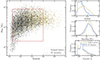 |
Fig. 1. Comparison of the properties of the two subsamples before trimming: blue for supercluster members and yellow for isolated clusters. The red rectangle in the left panel defines the M − z space where we select the subsamples for further selection (trimming). The histograms in the right panel show the distribution of redshift, mass, and exposure time of the two subsamples before the trimming process. |
In addition to the selection effects on redshift and mass, the fact that the clusters in the two subsamples are located at different survey depths also has non-negligible effects on the detection of assembly bias when concentration is adopted as the proxy for assembly history. A feature of X-ray surveys is that the selection of clusters is not a simple function of flux, but is affected by surface brightness patterns, such as the existence of a bright cool core, or more generally, the concentration or morphology of X-ray emission. The shallower the survey is, the more impact it suffers from these surface brightness patterns. This is because clusters with relatively flat surface brightness profiles have larger probabilities of being hidden in the background. As a comparison, cluster surveys based on the Sunyaev–Zeldovich (SZ) effect are less sensitive to surface brightness patterns because the SZ signal is almost a linear function of ne, instead of  for X-ray emission. As a consequence of this feature, ROSAT All-Sky Survey-based cluster samples are found to contain larger fractions of cool-core clusters than SZ-based samples, a phenomenon called “cool core bias” (e.g., Rossetti et al. 2017; Andrade-Santos et al. 2017). The hypothesis that this is related to survey depth is supported by the recent results that the cool core fraction of eFEDS clusters is lower than that of the ROSAT clusters, and is closer to SZ clusters (Ghirardini et al. 2022), probably because eFEDS has enough depth and better angular resolution to avoid the cool core bias found with ROSAT clusters. These results indicate that the selection effects induced by the inconsistent survey depths of the two subsamples should be taken into account in our analysis.
To construct two subsamples with consistent selection functions that are eligible for a direct comparison of concentration, we needed to correct for the above selection effects: We only considered the clusters within the redshift range 0.05 < z < 0.6 and the mass range 2 × 10¹³ M⊙ < M500 < 8 × 10¹⁴ M⊙ (see the left panel of Fig. 1), where we have enough statistics for both supercluster members and isolated clusters. All the clusters in our sample have an exposure time, t, in the range [60–2520 s], while the survey area rapidly decreases at deep exposures. With the cuts on mass and redshift, the sample size decreases from 8862 to 7658 (3577 SC members and 4081 isolated clusters). Then, we trimmed the two subsamples in the mass-redshift-exposure (M − z − t) space. The M − z − t space is divided into 50 × 50 × 8 = 20 000 3D grids. For mass and redshift, the boundaries of the grids are equally spaced in log- and linear-space, respectively. For exposure time, the following eight grids are manually chosen (in units of seconds): [60–150, 150–250, 250–350, 350–500, 500–700, 700–1000, 1000–1500, 1500–2520]. The edges are optimized to minimize each grid’s width while including enough clusters. In each M − z − t grid, we randomly selected the same number of supercluster members and isolated clusters. In each randomization, 1302 unique clusters were selected for both supercluster members and isolated clusters. Since there are often different numbers of supercluster members and isolated clusters within one grid, the lists of clusters being selected in each randomization may differ from each other. To obtain stable results of selection, the randomization is repeated 1000 times, and the lists of clusters from each randomization are merged. We thus constructed subsamples of supercluster members and isolated clusters, each consisting of 1302 × 1000 clusters. However, each subsample only contains about 1700 unique clusters, since most clusters are selected multiple times. Therefore, we weighted each unique cluster in the two subsamples with the frequency of being selected when computing any average values.
With the trimming approach described above, we established two unbiased subsamples of clusters, namely, supercluster members and isolated clusters, with the same redshift distribution, mass distribution, and survey depth. Each subsample contains about 1700 clusters. Specifically, the median values of redshift, mass, and exposure time for SC members and isolated clusters for the trimmed subsamples are [0.2376, 0.2374], [1.90 × 10¹⁴ M⊙, 1.89 × 10¹⁴ M⊙], and [142.1 s, 142.2 s], respectively. Thus, the differences are negligible and the two subsamples can be directly compared without significant selection effects. The consistency of the two subsamples is demonstrated in Fig. 2. We did not apply the trimming process to other quantities except for redshift, mass, and exposure time. Other factors such as the discrepancy in the Galactic hydrogen column density, nH, of the two subsamples may also have very minor impacts on the results. However, in the construction of the eRASS1 galaxy cluster sample, we excluded most of the Galactic disk areas, and the majority of the clusters are located at high Galactic latitudes where the nH is relatively low. Therefore, the effect of nH should be negligible compared to the impacts of redshift, mass, and survey depth (Kluge et al. 2024).
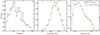 |
Fig. 2. Comparison of the properties of the two subsamples after trimming. The histograms show the distribution of redshift, mass, and exposure time, from left to right. Supercluster members and isolated clusters are plotted in blue and yellow, respectively. |
3. Comparison of gas mass concentrations
After obtaining the bias-free subsamples of supercluster members and isolated clusters, we could investigate their differences in halo properties. In this work, we adopted gas mass concentration as the proxy for halo assembly history. We simply defined the gas mass concentration as the ratio of gas mass within two radii: cgas ≡ Mgas(r1)/Mgas(r2), where r1 = 0.3 R500 and r2 = R500.
The cgas for the clusters can be obtained from the X-ray analysis performed in Bulbul et al. (2024). The eRASS1 X-ray data are processed with the eROSITA Science Analysis Software System (eSASS; Brunner et al. 2022)5. We used the tool MultiBand Projector in 2D (MBProj2D, Sanders et al. 2018)6 to measure the gas properties of the eRASS1 clusters by fitting multiband X-ray images. By forward-fitting background-included X-ray images of a galaxy cluster, MBProj2D provides the physical models of the cluster, such as the electron density profile, temperature profile, and metallicity profile (see, e.g., Liu et al. 2023, for a recent application of MBProj2D). In the analysis of eRASS1 clusters, we divided the energy range [0.3–7] keV into seven bands (in units of keV): [0.3–0.6], [0.6–1.0], [1.0–1.6], [1.6–2.2], [2.2–3.5], [3.5–5.0], [5.0–7.0], to be able to constrain the ICM temperature. Counts images and exposure maps are created in these bands to be fitted with MBProj2D. When there are multiple clusters in the image, all the clusters are properly fitted instead of masked, to make sure that the background emission cannot be systematically boosted by the residual emission from neighboring clusters. This is particularly important for the analysis of supercluster members. We used all seven telescope modules in the analysis. However, telescope modules 5 and 7 are ignored for the soft energy band below 1 keV, because they are affected by light leak (Predehl et al. 2021). The density profile is described using the model from Vikhlinin et al. (2006), but without the second β component:
Here ne and np are the number densities of electron and proton, and we assume ne = 1.21 np. n0, rc, α, β, γ, rs and ϵ are free parameters. Gas density and gas mass profiles are then computed from the electron density profiles: ρg = nempA/Z, where A ∼ 1.4 and Z ∼ 1.2 are the average nuclear charge and mass for ICM when assuming a metallicity of 0.3 Z⊙ (e.g., Mernier et al. 2018; Bulbul et al. 2016).
The median electron density profiles of supercluster members and isolated clusters are plotted in Fig. 3. To quantify the difference between the two classes of clusters (if any), we constructed two control samples by randomly dividing the clusters into two subsamples S1 and S2, and applied the same trimming process described above. This approach was repeated 1000 times, and thus the standard deviation of the excess in cgas of S1 over S2 represents the uncertainty in that of supercluster members and isolated clusters due to randomization. The median electron density profiles of S1 and S2 are also shown in Fig. 3.
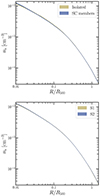 |
Fig. 3. Median electron density profiles. In the upper panel, the results for supercluster members and isolated clusters are plotted in blue and yellow, respectively. The uncertainties of the two profiles are almost negligible due to the large number of clusters in each sample. The difference in gas mass concentration between the two samples is almost invisible. In the lower panel, we plot the results for the two control samples, which are selected by randomly dividing the cluster sample into two. |
From Fig. 3, we observe no obvious difference between supercluster members and isolated clusters in their electron density profiles. Quantitatively, the median cgas is 0.160 and 0.155 for isolated clusters and supercluster members, respectively. Thus, if we quantify the HAB signal with the excess in cgas of isolated clusters over supercluster members, δcgas ≡ cgas, ISO/cgas, SC − 1, then we obtain δcgas = 0.031. As a comparison, the standard deviation of cgas, S1/cgas, S2 − 1 is 0.019 (see Fig. 4). Therefore, our result on δcgas is only at a confidence level of 1.6σ, corresponding to a marginal signal of HAB.
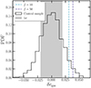 |
Fig. 4. Confidence level of the excess in gas mass concentration, cgas. The histogram shows the distribution of δcgas defined as cgas, S1/cgas, S2 − 1 when randomly dividing the clusters into two subsamples (S1 and S2) and repeating 1000 times. The dashed lines indicate the δcgas when the clusters are divided into supercluster members and isolated clusters. The results are shown for different overdensity ratios in the identification of superclusters. The shaded area represents 1σ uncertainty. The cyan and purple lines correspond to 1.6σ for f = 10 and 2.0σ for f = 50, respectively. |
We further investigated whether the low magnitude of HAB is due to the criterion we used to identify superclusters, namely, overdensity ratio f = 10. In Liu et al. (2024), we also provide a supplementary catalog of superclusters, identified with the same FoF method on the eRASS1 galaxy cluster catalog, but using a stricter criterion of overdensity: f = 50. This supplementary catalog includes 929 supercluster systems and 2205 supercluster members. We performed the same selection and trimming approaches described in Sect. 2 on the f = 50 supercluster sample. After these processes, we obtain 956 supercluster members and 1269 isolated clusters for a direct comparison. We note that the notation “isolated clusters” indicates clusters that are not members of superclusters in the f = 10 catalog or the f = 50 catalog. Namely, we excluded the clusters between f = 10 and f = 50, which are supposed to have intermediate clustering magnitudes. The median electron density profiles of the f = 50 sample are shown in Fig. 5. Compared to the results of the f = 10 sample, the enhancement in the difference of the electron density profiles is almost negligible. The median cgas of isolated clusters and supercluster members are 0.159 and 0.153, respectively. The significance of δcgas is increased from 1.6σ to 2.0σ (see Fig. 4). Therefore, we detect a subtle HAB signal with both the f = 10 and f = 50 supercluster samples.
It is also important to check if the signal is simply caused by merging clusters in the supercluster systems. We are more interested in the behavior of concentration as a proxy for cluster assembly history, instead of being a simple indicator of its current merging stage. Clusters that are currently undergoing merger activities naturally have more flattened gas distributions and are more likely to be identified as superclusters due to their small distances from neighbors. Therefore, we repeated our analysis by conservatively removing any cluster that intersects with a neighbor within their R500 on the plane of the sky. Among the 8862 clusters in the sample, 741 clusters (about 8%) are excluded. The minimum distance between any clusters in the remaining sample is larger than the sum of their R500. Using this merger-free sample, we obtain cgas, ISO = 0.161, cgas, SC = 0.156, δcgas = 0.032 ± 0.021 for f = 10, and cgas, ISO = 0.161, cgas, SC = 0.153, δcgas = 0.051 ± 0.024 for f = 50. The results are in very good agreement with the full sample. We can thus rule out the hypothesis that the HAB signal is simply caused by clusters that are currently undergoing mergers.
3.1. The impact of concentration on sample selection
The masses of the eRASS1 clusters within R500 are computed using the weak-lensing-calibrated scaling relation between the X-ray count rate within R500 (CR500), redshift, and mass M500. This is very similar to the widely used M − LX scaling relation, but we used count rate instead of luminosity because the former is more correlated with the selection procedure of the eRASS1 clusters. Since the core emission is also included in the scaling relation, the mass computation can be affected by gas concentration. In general, the masses of the clusters with higher gas mass concentrations can be slightly biased toward higher values, due to the X-ray surface brightness being proportional to  and thus is boosted by the bright core. This effect is minor and well below the typical error bar of our mass measurements. However, since we aim to detect faint signals of only a few percent, we carefully checked the impact of the mass-concentration correlation on our sample selection. The ideal solution for this issue is to measure the mass profile independently from the weak-lensing shear profile for each cluster in the sample. However, the signal-to-noise of individual shear profiles is too low for most of our clusters. Another commonly accepted solution is to exclude the core in the computation of scaling relations. This has been proved by recent studies, where the scatter in M − LX scaling relation is found to be smaller for core-excised luminosities (see, e.g., Bulbul et al. 2019).
Since our only aim is to avoid a mass discrepancy between the two subsamples, instead of obtaining absolute mass measurements, there is no need to establish the M − Lcex scaling relation and recompute the masses from core-excised luminosities. Given the two subsamples already have the same redshifts, the only necessary step is to make sure they are also consistent in core-excised luminosity, Lcex. Therefore, the trimming process on Lcex is already sufficient for our purpose.
We then repeated the selection and trimming processes described in Sect. 2, but in (L500, cex, z, t) space instead of (M − z − t). In this work, we defined the core size as 0.3 R500 to be consistent with our definition of gas mass concentration. We divided the L500, cex range [1041 − 3 × 1044 erg/s] into 50 bins in log-space. The selections on redshift and exposure time remain the same as described in Sect. 2. The calculations based on control samples were also repeated accordingly. As a result, we obtain a median cgas of 0.155 and 0.152 for isolated clusters and supercluster members, respectively. Therefore, the significance of concentration excess δcgas = 0.020 ± 0.018 is only at 1.1σ. If we further investigate the f = 50 supercluster sample, then we obtain δcgas = 0.031 ± 0.018. Therefore, the significance of δcgas is increased to 1.7σ, close to the results obtained with count rate CR500 as the mass proxy. These results also indicate that the mass-concentration correlation only has negligible impacts on our sample selection.
3.2. Results for different mass and redshift ranges
According to several previous works, HAB is stronger for low-mass halos than massive halos, or behaves differently in low- and high-mass regimes (e.g., Wechsler et al. 2006). Therefore, we further checked the results when we divided the cluster sample into two mass ranges. We cut the sample at M500 = 2 × 10¹⁴ M⊙, and applied the same selection and trimming processes described in Sect. 2. We then performed the same experiments as for the whole sample. The δcgas were obtained for different over density ratios f = 10 and f = 50, and for different mass proxies CR500 and L500, cex. Due to the cut on mass, the number of clusters is reduced by ∼50% for each of the low-mass and high-mass samples compared to the whole sample. This further leads to a larger error bar in δcgas. Therefore, it is expected that the significance of the results will be even lower than the whole sample, although the hints we obtain from the comparison between low- and high-mass regimes will still be useful.
In general, we find a decreasing trend in δcgas with the investigated mass ranges. For the low-mass sample, we obtain larger δcgas than the whole sample. For the high-mass sample, δcgas is lower than both the low-mass sample and the whole sample, indicating that the difference in cgas of supercluster members and isolated clusters is almost negligible for massive clusters above 2 × 10¹⁴ M⊙. However, this trend needs to be confirmed by further studies due to the large error bar of the measurements (see Sect. 5.2).
We also investigated the results for different redshift ranges by dividing the whole sample into a low-z sample (0.05 < z < 0.2) and a high-z sample (0.2 < z < 0.6). δcgas is enhanced to 6%–8% for the low-z sample. Specifically, we obtain δcgas = 0.080 ± 0.028 for f = 10 and δcgas = 0.069 ± 0.032 for f = 50. As a comparison, the HAB signal completely disappears for the high-z sample, where we obtain δcgas = −0.006 ± 0.028 for f = 10 and δcgas = 0.000 ± 0.030 for f = 50. This redshift trend could partially originate from the mass trend because the low-z sample contains most of the low-mass clusters, and the high-z sample is dominated by massive clusters. However, another possibility is that the large-scale environment continuously affects the assembly of clusters, and the HAB signal tends to increase with time. We further split the low-z clusters into a low-mass sample and a high-mass sample. Unsurprisingly, we obtain from the low-z low-M sample the largest δcgas among all the experiments: 0.106 ± 0.039. As a comparison, the low-z high-M sample has δcgas = 0.066 ± 0.036, lower than the result for low-z low-M clusters but still higher than that for the high-M sample without redshift cut. These results, if tied together, suggest an increasing trend of δcgas at both lower masses and lower redshifts. The only missing part in this scenario is the case of low-mass clusters at high redshifts, most of which are below the eRASS1 flux limit and not included in our sample. This will be improved in the future with deeper eROSITA surveys (see Sect. 5.2).
The results from all the experiments described above are summarized in Fig. 6 and Table 1.
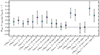 |
Fig. 6. Summary of the results for δcgas obtained in this work for different choices of overdensity ratio f in supercluster identification, cluster mass proxy, and mass range. The results for f = 10 and f = 50 are plotted in cyan and purple, respectively, to show the increasing trend in δcgas with f. The two measurements for the total mass concentration obtained from weak-lensing analysis, |

Our cgas and ctot results for supercluster members and isolated clusters.
4. Comparison of total mass concentrations
To compare with the gas mass concentration results, we also attempted to use total mass concentration as the proxy of halo assembly history. Due to the different dynamic characteristics of the collisionless dark matter particles and the viscous intracluster gas, the absolute values of the total mass and gas mass concentrations are not comparable with each other, but the trends in δcgas and δctot are expected to be consistent. Although the weak-lensing shear profiles for individual clusters are too noisy to measure concentration, we can use the stacked shear profile to obtain the average mass concentration for a sample of clusters. We performed this experiment for the two samples with f = 10 and f = 50, after applying the same trimming process described in Sect. 2. We used the public Dark Energy Survey year 3 (DES-Y3) data to measure the stacked shear profiles for supercluster members and isolated clusters, respectively. The numbers of SC members and isolated clusters in the DES footprint are 735 and 627 for f = 10, and 418 and 437 for f = 50.
In the weak-lensing formalism, the tangential gravitational shear, γt, induced by the foreground structure (lens; galaxy clusters in this case) is related to the surface density of the lens, Σ(R), as

where
and

Here, zl and zs are the redshifts of the lens and the source. DA, l, DA, s and DA, ls are the angular diameter distances to the lens, to the source, between the lens and the source, respectively.  is the mean surface density within the radius R from the center of the lens. We note that the tangential shear is related to the two shear components, γ1 and γ2, as

where θ is the position angle of the galaxy with respect to the x-axis of the system.
For the weak-lensing measurement, we used the shape catalog from the DES-Y3 data measured by METACALIBRATION algorithm (Sheldon & Huff 2017; Huff & Mandelbaum 2017; Gatti et al. 2021). In METACALIBRATION, the true shear, γ, is related to the measured galaxy shape, e through the response matrix, ℛ,
We also calculated and included the selection response, ℛs, which arises due to the specific selection of galaxies. We refer the readers to the above studies for further details.
We adopted the photometric redshifts of the galaxies measured by the DNF algorithm taken from the DES-Y3 Gold catalog (Sevilla-Noarbe et al. 2021). We made use of the two different redshift values for each galaxy as given by the catalog – the mean estimated redshift (zmean) and a redshift value randomly chosen from the probability distribution (zMC). For further details, we refer the readers to Sevilla-Noarbe et al. (2021) and the references therein.
In principle, the measured gravitational shear by METACALIBRATION could be multiplicatively biased. Furthermore, due to the large uncertainty of the photometric redshift of the source galaxies, the weak-lensing measurement is subject to another multiplicative bias through Σcrit (e.g., McClintock et al. 2019). However, since our main goal is to compare the concentration (not the mass) of the supercluster members to that of the isolated clusters, and those multiplicative biases apply to all samples equally, we did not include these bias factors in our analysis. We also ignored the uncertainty on the cluster redshift since it is significantly smaller than that of the source galaxies.
Following McClintock et al. (2019) and Shin et al. (2021), we constructed our estimator for ΔΣ(R) as
where
Here, i runs over the lens clusters, and j runs over the source galaxies. et is the tangential component of the measured galaxy shape. Also,  is evaluated with the redshift of the source galaxies using zMC, while for
  zmean is used. In addition, ℛt is the tangential component of the response matrix rotated to the tangential coordinate, and σγ is the uncertainty of the shape measurement. We refer the readers for this estimator’s details and validation to McClintock et al. (2019).
To minimize the contamination from the foreground or cluster member galaxies that do not carry any lensing signal, we selected source galaxies such that zs > zl + 0.1 using the photo-z from DNF. However, due to the high uncertainties on the photometric redshifts of the galaxies, the cluster member galaxies that do not carry any lensing signal could leak into our source galaxy selection, which dilutes the weak-lensing signal. Therefore, one must measure and take into account this scale-dependent systematic bias in the analysis. This is generally called the “boost factor”, ℬ(R), which we modeled following the method outlined in Gruen et al. (2014) and Varga et al. (2019) as follows.
For a measured photometric redshift distribution at the cluster-centric distance of R, P(z|R), we decomposed the distribution into the cluster contamination, Pcont(z), and the true background distribution, Pbg(z):

We note that fcl(R), a free parameter per radial bin, represents the fraction of member galaxy contamination in the distribution, and we modeled Pcont(z) as a radius-independent Gaussian distribution with a mean (μz, cl) and a standard deviation (σz, cl) as additional free parameters. The corrected weak-lensing profile after accounting for the boost factor becomes,
We modeled the 3D cluster mass profile as,

where ρNFW = ρcritδc/[(r/rs)(1 + r/rs)2] is a Navarro-Frenk-White profile (Navarro et al. 1997) for which we have two free parameters: the total mass, M500, and the concentration, C500 = R500/rs. The second term is so-called the two-halo contribution due to the nearby halos that are clustered, where ρm(z) is the mean matter density of the Universe at the redshift z, ξmm(r|z) is the matter-matter correlation function of the Universe at z with the separation of r, and bc is the large-scale halo bias (Tinker et al. 2010) that is another free parameter in our model. We then integrated this 3D density model into 2D along the line of sight to obtain the 2D projected surface mass density, Σ(R).
On the other hand, the X-ray centers used here could be offset from the true centers of the halos. Therefore, we included the miscentering effect in our model. For a given set of clusters, the stacked surface density profile in the presence of miscentering can be expressed as,

where fmis is the fraction of the miscentered clusters, Σ0 the surface density profile without any miscentering, and Σmis) the profile with miscentering, which can be expressed as
Here, Rmis is the miscentered distance, and we assumed a Rayleigh distribution for P(Rmis),
By geometry, one can also show that the profile of a halo that is miscentered by Rmis is

Grandis et al. (2024) provide the average miscentering properties for the eROSITA clusters. However, since our goal is to compare the properties of supercluster members and isolated clusters, for each of which the miscentering properties are not well studied, we adopted flat priors for the two miscentering parameters, fmis = [0, 1] and lnσR = [0.05, 0.5].
We measured the  (Eq. (8)) in 16 logarithmically spaced radial bins between 0.1 and 10.0 h−1 Mpc in physical unit. The P(z|R) of each radial bin for the boost factor fitting is calculated with redshift bins between z = 0.05 and 1.25 with the bin width of Δz = 0.05. Pbg(R) is calculated around the random positions within the survey footprint (N = 30 times the number of clusters).
The covariance matrix of  is obtained by bootstrapping the clusters with 100 000 bootstrapped samples. For each bootstrapped cluster sample, we obtain the best-fit boost factor parameters (μz, cl, σz, cl, fcl(Ri)) by fitting the observed P(z|R) to the model described above. Then this bootstrapped boost factor is multiplied to the corresponding bootstrapped
  , from which we obtain our final boost-factor-corrected
  with its covariance matrix.
We then performed Markov chain Monte Carlo (MCMC) analyses on the corrected weak-lensing profile to get the constraints on the halo properties, for which we have five free parameters, M500, C500, bc, fmis, and σR. We fixed the redshift of the model to the mean cluster redshift and assume a Gaussian likelihood for the fitting. We used EMCEE package (Foreman-Mackey et al. 2013) to obtain the MCMC chains.
The measured weak-lensing profiles with the boost factor correction as a function of cluster-centric radius are shown in Fig. 7. The top panels show the ΔΣ profiles for the f = 10 sample (left) and the f = 50 sample (right); in both the isolated clusters (yellow) show higher amplitudes below 0.7 h−1 Mpc than that of the supercluster members (blue), hinting at a higher value of concentration for the isolated clusters. The 68% confidence intervals of the best-fit model for each measurement are shown with the shaded bands with the corresponding colors, with the best-fit models plotted with the dashed lines of the same colors. For the f = 10 (f = 50) sample, the best-fit χ2 per degree of freedom for the supercluster members is 9.0/11 (14.9/11) corresponding to the probability to exceed (PTE) of 0.62 (0.18), while that for the isolated clusters is 14.7/11 (16.7/11) corresponding to PTE = 0.20 (0.12). In the middle panels, we show as a null test the cross-components of the weak-lensing measurements, defined as

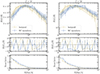 |
Fig. 7. Measured weak-lensing ΔΣ profiles (top), the cross components for a null test (middle), and the boost factors (bottom) for the f = 10 sample (left) and the f = 50 sample (right). The supercluster members are plotted in blue and the isolated clusters in yellow. The shaded regions represent the 68% confidence best-fit interval, while the dashed lines correspond to the best-fit models. |
substituting γt, which must be consistent with zero for the isotropic lens. The minimum of χ2 per degree of freedom for f = 10 (f = 50) sample is 12.1/16 (12.9/16) for the supercluster members and 16.1/16 (21.3/16) for the isolated clusters, which are consistent with zero. Finally, the bottom panels show the measured boost factors with the same color scheme, where the supercluster members and the isolated clusters show features distinct from each other, while they both asymptote to 1 at large scales as expected. We defer a detailed analysis of the difference in the galaxy number density profile between the two samples, as suggested by the boost factors, to future studies.
In Appendix A we show the corner plots of the MCMC run for the f = 10 (Fig. A.1) and f = 50 samples (Fig. A.2). For both cases, the supercluster members and the isolated clusters exhibit similar masses (M500), within 1σ of each other, while the isolated clusters have a larger concentration (C500) than that of the supercluster members, in alignment with our previous findings. Using these chains, we then obtained the concentration of the total mass ctot with the same definition of cgas (ctot = M(< 0.3 R500)/M500). For the f = 10 supercluster sample, the total mass concentrations ctot of the supercluster members and isolated clusters are  and
and  , respectively, corresponding to
  . For the f = 50 supercluster sample, we obtain
  ,
,  , with δctot of
  . As expected, the absolute values of total mass concentrations are larger than gas mass concentrations, since dark matter particles are collisionless and the ICM is viscous. On the other hand, for both cases, we observe the same trend as gas mass concentration, that supercluster members are also less concentrated than isolated clusters in total mass. The significance level of δctot is 1.5σ, slightly lower than that of δcgas, possibly because only < 40% of the clusters are within the DES footprint and included in the weak lensing analysis. We also note that the posteriors for the miscentering parameters are wide and poorly constrained, so that by marginalizing over those parameters we enhance the robustness of our finding at the cost of less precision. It is also noticeable that the posteriors for the large-scale halo bias parameter (bc) are almost identical between supercluster members and isolated clusters, indicating that the HAB is not detected at the large-scale halo bias level, but only at the concentration level. We note, however, that our analysis is limited to R < 10 h−1 Mpc, and therefore may not be suitable for probing such large-scale bias signals. We defer a more detailed study on this matter to a future study.
5. Discussions
In this section, we provide possible interpretations of our findings and discuss potential improvements to our results in the near future when deeper eRASS data are available.
5.1. Interpretation of the results
As presented in the previous sections, in all the experiments we performed, we consistently observed a trend that supercluster members have lower concentrations, both in gas mass and total mass, than isolated clusters. This result is rather stable over a series of choices on cluster mass proxy, supercluster overdensity ratio, and cluster mass range. We also find that the concentration excess of isolated clusters compared to supercluster members (δcgas and δctot) increases marginally when we choose a higher threshold on the overdensity ratio of supercluster identification, implying that the difference in concentration is likely related to environmental effect. Although the significance level of any single experiment is not high enough (the maximum significance of δcgas is 2.8σ), these results are indeed in line with our current understanding of HAB based on many previous works on numerical simulations, where HAB is detected for massive halos. In these works, halos with higher clustering magnitudes are found to be less concentrated (e.g., Wechsler et al. 2006; Wetzel et al. 2007; Gao & White 2007).
To understand and interpret the signal we detected in this work, we first revisited the physical origin of HAB proposed by previous works. As already mentioned in Sect. 1, a widely accepted explanation for HAB of low-mass halos is that the tidal fields of the neighboring massive halos prevent the low-mass halos from accreting matters. For example, Wang et al. (2007) found that low-mass old halos are often located close to more massive halos. The gravitational tidal fields of the neighboring massive halo produce a hot environment (e.g., Mo et al. 2005), which suppresses the mass accretion of the low-mass halos, and leads to the old ages of these low-mass halos. In this scenario, the environmental effect should generally decrease with halo mass. More massive halos dominate their vicinity and their evolution is less affected by the environment. This implies that the signal of HAB should be much weaker in clusters, which is consistent with our results. Moreover, the fact that we are observing systematically larger δcgas in the low-mass sample, despite the large error bar, is also in line with the above scenario.
Another scenario is that supercluster members are less concentrated simply because they are located in denser regions and thus have experienced more mergers during their assembly history. Merging processes between clusters can significantly flatten the distributions of both the baryon and dark matter components; thus, supercluster members are expected to have lower concentrations than isolated clusters in both the gas mass and total mass. Compared to low-mass clusters, massive clusters are less affected by minor mergers, while the occurrence of major mergers is much rarer compared to minor mergers, which provides an explanation of the trend that δcgas marginally decreases with mass. Moreover, since mergers between clusters occur continuously, it can be inferred that the strength of HAB signal increases with time, which is consistent with the larger cgas we find for low-z clusters. Therefore, the environmental dependence of cluster merger rates can also interpret our results and should be regarded as another possible origin of HAB.
5.2. Expected improvements with deeper eRASS data and multiwavelength cluster surveys
The next question is how we can improve the significance of the detection of HAB. An effective way to increase the significance of the signal is to expand the sample of supercluster members. eROSITA has completed more than four all-sky surveys. About 5 × 10⁴ clusters and groups are expected to be detected in eRASS:4. Using the same criteria in supercluster identification, we expect to expand the sample of supercluster members by a factor of four. With the deeper X-ray data, the uncertainty in the measurements of electron density profiles will also be reduced significantly. Therefore, with the eRASS:4 data and cluster sample, we expect to improve the significance of the HAB signal by at least a factor of three, corresponding to a detection at 6σ confidence level for the full sample without mass and redshift cuts. eRASS:4 will also significantly expand the sample of low-mass clusters at high redshifts, and further confirm the mass and redshift dependences of HAB we find in this work.
Another approach is to make joint analyses by including the samples of clusters and superclusters detected in other wavelengths, such as optical and the millimeter to submillimeter (SZ effect). Cluster samples selected in different bands have their advantages and disadvantages. Optical cluster samples are more complete than X-ray and SZ samples, although the purity is usually lower, and the selection function is more complicated. SZ cluster samples contain fewer contaminants (e.g., projected interlopers in the optical and AGNs in the X-ray), and have a simpler selection function directly correlated with cluster mass. However, limited by the much lower angular resolution of SZ telescopes, SZ observations provide fewer constraints compared to X-rays on cluster properties such as gas mass concentration. Therefore, combining these cluster samples and the multiwavelength observations would help establish a more comprehensive dataset to study HAB with superclusters. We note that an essential step in such an approach is to carefully account for the selection effects in each band and each survey. As an example, we show in Fig. 8 how sensitive is the detection of HAB to the selection effects in our eRASS1 X-ray survey. We plot the electron density profiles of the supercluster members and the isolated clusters obtained in the same way as plotted in the left panel of Fig. 3, but without applying the trimming process on the exposure time. Namely, the two subsamples are consistent in both redshift and mass but have different survey depths. In this case, the difference in gas mass concentration is visible in the plot and would be misinterpreted as the “signal” of HAB if we do not exclude the selection effect caused by the inhomogeneity in survey depth. This plot showcases the importance of correcting selection effects in the exploration of HAB with large-area surveys.
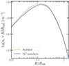 |
Fig. 8. Same as the left panel of Fig. 3 but without considering the difference in exposure time of the supercluster members and isolated clusters. The y-axis is rescaled by the radius to reduce the dynamic range of the plot and improve the visibility of the difference between the two samples. The median electron density profile of supercluster members (blue) shows an apparently lower concentration than that of the isolated clusters (yellow). However, this trend should not be simply interpreted as the signal of HAB. It is mostly caused by the fact that supercluster members are located in areas with higher survey depths, where low-concentration clusters have a higher probability of being detected. This plot demonstrates the importance of correcting for selection effects in the analysis of HAB. |
6. Conclusions
We propose a novel method for exploring HAB in cluster-sized halos. The essence of this method is to use superclusters to identify the clusters that are located in denser environments and with higher clustering magnitudes (namely, supercluster members) and compare their assembly history with that of isolated clusters, to investigate the environmental effect on halo assembly history. In this work, we applied this method to the largest-ever X-ray galaxy cluster and supercluster samples obtained from eRASS1 (Bulbul et al. 2024; Kluge et al. 2024; Liu et al. 2024). We constructed two subsamples of galaxy clusters, which consist of supercluster members and isolated clusters, respectively. A “trimming” approach was applied to the two subsamples to overcome selection effects and ensure the two subsamples are consistent in redshift, mass, and survey depth. The concentration of the ICM, defined as the ratio of gas mass within 0.3 R500 and R500, was adopted as the proxy of the halo assembly history. The HAB signal was quantified with the excess in the gas mass concentration of isolated clusters compared to supercluster members: δcgas ≡ cgas, ISO/cgas, SC − 1. We obtained δcgas under multiple conditions, including different overdensity ratios for supercluster identification, cluster mass proxies, cluster mass ranges, and redshift ranges. We also performed weak lensing analysis on the two subsamples. By stacking the weak lensing shear profiles of the clusters in each subsample, we compared the concentrations of the total mass, δctot, defined in the same way as the gas mass concentration.
We find that the average gas mass concentration of isolated clusters is a few percent higher than that of supercluster members. The δcgas result varies depending on our choices for the supercluster overdensity ratio, f, and mass and redshift ranges but remains positive in almost all cases. Specifically, we measure slightly higher δcgas when adopting the supercluster sample identified with higher f, which, by definition, corresponds to higher clustering magnitudes and selects clusters in denser environments. These results are also supported by the comparison of total mass concentrations between the two samples, measured from the weak lensing analysis, which shows similar trends as the results obtained from the gas mass. By dividing our cluster sample into subsamples based on mass and redshift, we also find that δcgas is higher for clusters with lower masses and at lower redshifts. Our findings are consistent with the prediction of HAB on cluster scales, where halos located in denser environments are less concentrated than isolated ones, and this trend is stronger for less massive and low-redshift halos. These phenomena can be explained by the fact that clusters in denser environments such as superclusters have experienced more mergers than isolated clusters in their assembling history.
Among all the measurements we obtained in this work, the maximum confidence level of δcgas or δctot is 2.8σ, only corresponding to a marginal signal of HAB. Therefore, the results from this first attempt to explore HAB with superclusters are not conclusive enough to end the debate on the existence of HAB for cluster-sized halos. In the near future, the results of this work are expected to be improved upon thanks to deeper eROSITA surveys, which will significantly expand the sample of both supercluster members and isolated clusters, and improve the quality of the X-ray data. This work paves the way to explore HAB with superclusters, and demonstrates that large samples of superclusters, a category of object in the Universe that has been known for decades, can advance our understanding of the evolution of the large-scale structure. With the methodology we have laid out in this work, a joint analysis combining optical and SZ cluster and supercluster samples will also provide useful constraints on HAB on cluster scales. However, we stress that the selection effects of different cluster surveys must be carefully accounted for in the investigation of HAB.
It should be noted that superclusters identified with X-ray cluster surveys are usually open structures without strict physical boundaries. In the most extreme case, the Universe can be regarded as a “large supercluster”. Therefore, there is no absolute dividing line between “supercluster members” and “isolated clusters”. The division of these two classes depends on the parent X-ray cluster sample and the criteria for supercluster identification. There are attempts to define superclusters as the systems that will survive the cosmic expansion and eventually collapse, based on their overdensities (see, e.g., Chon et al. 2015). However, predicting whether a supercluster will collapse from the estimation of its overdensity is highly uncertain. Even for the simplest cases of superclusters, namely, cluster pairs (except for those compact pairs in the merging process), observationally verifying such predictions would at least require accurate measurements of the peculiar velocities of the member clusters and their distance, which are not available for most of the currently known supercluster systems. Definitions for supercluster boundaries are also proposed in other domains, for example, optical galaxy surveys or simulations (e.g., Einasto et al. 2019; Dupuy et al. 2019). However, these definitions may not apply to X-ray cluster surveys.
Acknowledgments
We greatly thank the anonymous referee for his/her constructive comments. AL thanks Daisuke Nagai, Stefano Borgani, and Stefano Ettori for helpful discussions. This work is based on data from eROSITA, the soft X-ray instrument aboard SRG, a joint Russian-German science mission supported by the Russian Space Agency (Roskosmos), in the interests of the Russian Academy of Sciences represented by its Space Research Institute (IKI), and the Deutsches Zentrum für Luft- und Raumfahrt (DLR). The SRG spacecraft was built by Lavochkin Association (NPOL) and its subcontractors and is operated by NPOL with support from the Max Planck Institute for Extraterrestrial Physics (MPE). The development and construction of the eROSITA X-ray instrument was led by MPE, with contributions from the Dr. Karl Remeis Observatory Bamberg & ECAP (FAU Erlangen-Nuernberg), the University of Hamburg Observatory, the Leibniz Institute for Astrophysics Potsdam (AIP), and the Institute for Astronomy and Astrophysics of the University of Tübingen, with the support of DLR and the Max Planck Society. The Argelander Institute for Astronomy of the University of Bonn and the Ludwig Maximilians Universität Munich also participated in the science preparation for eROSITA. The eROSITA data shown here were processed using the eSASS/NRTA software system developed by the German eROSITA consortium. Ang Liu, Esra Bulbul, Vittorio Ghirardini, and Xiaoyuan Zhang acknowledge financial support from the European Research Council (ERC) Consolidator Grant under the European Union’s Horizon 2020 research and innovation program (grant agreement CoG DarkQuest No. 101002585). Nicola Malavasi acknowledges funding by the European Union through a Marie Skłodowska-Curie Action Postdoctoral Fellowship (Grant Agreement: 101061448, project: MEMORY). Views and opinions expressed are however those of the author only and do not necessarily reflect those of the European Union or of the Research Executive Agency. Neither the European Union nor the granting authority can be held responsible for them. This research was partially supported by the Excellence Cluster ORIGINS which is funded by the Deutsche Forschungsgemeinschaft (DFG, German Research Foundation) under Germany’s Excellence Strategy – EXC 2094 – 390783311. TS and AvdL are supported by the US Department of Energy under award DE-SC0023387. This work made use of SciPy (Jones et al. 2001), Matplotlib, a Python library for publication-quality graphics (Hunter 2007), Astropy, a community-developed core Python package for Astronomy (Astropy Collaboration 2013), NumPy (Van Der Walt et al. 2011).
References
- Adami, C., Giles, P., Koulouridis, E., et al. 2018, A&A, 620, A5 [NASA ADS] [CrossRef] [EDP Sciences] [Google Scholar]
- Andrade-Santos, F., Jones, C., Forman, W. R., et al. 2017, ApJ, 843, 76 [Google Scholar]
- Astropy Collaboration (Robitaille, T. P., et al.) 2013, A&A, 558, A33 [NASA ADS] [CrossRef] [EDP Sciences] [Google Scholar]
- Böhringer, H., & Chon, G. 2021, A&A, 656, A144 [NASA ADS] [CrossRef] [EDP Sciences] [Google Scholar]
- Bond, J. R., Cole, S., Efstathiou, G., & Kaiser, N. 1991, ApJ, 379, 440 [NASA ADS] [CrossRef] [Google Scholar]
- Borzyszkowski, M., Porciani, C., Romano-Díaz, E., & Garaldi, E. 2017, MNRAS, 469, 594 [NASA ADS] [CrossRef] [Google Scholar]
- Brunner, H., Liu, T., Lamer, G., et al. 2022, A&A, 661, A1 [NASA ADS] [CrossRef] [EDP Sciences] [Google Scholar]
- Bulbul, E., Randall, S. W., Bayliss, M., et al. 2016, ApJ, 818, 131 [Google Scholar]
- Bulbul, E., Chiu, I. N., Mohr, J. J., et al. 2019, ApJ, 871, 50 [Google Scholar]
- Bulbul, E., Liu, A., Kluge, M., et al. 2024, A&A, 685, A106 [NASA ADS] [CrossRef] [EDP Sciences] [Google Scholar]
- Chen, T. C., Lin, Y. T., Schive, H. Y., et al. 2024, ApJ, submitted [arXiv:2401.10322] [Google Scholar]
- Chon, G., Böhringer, H., & Nowak, N. 2013, MNRAS, 429, 3272 [Google Scholar]
- Chon, G., Böhringer, H., Collins, C. A., & Krause, M. 2014, A&A, 567, A144 [NASA ADS] [CrossRef] [EDP Sciences] [Google Scholar]
- Chon, G., Böhringer, H., & Zaroubi, S. 2015, A&A, 575, L14 [NASA ADS] [CrossRef] [EDP Sciences] [Google Scholar]
- Chue, C. Y. R., Dalal, N., & White, M. 2018, JCAP, 2018, 012 [Google Scholar]
- Dalal, N., White, M., Bond, J. R., & Shirokov, A. 2008, ApJ, 687, 12 [NASA ADS] [CrossRef] [Google Scholar]
- Diemand, J., Kuhlen, M., & Madau, P. 2007, ApJ, 667, 859 [NASA ADS] [CrossRef] [Google Scholar]
- Dupuy, A., Courtois, H. M., Dupont, F., et al. 2019, MNRAS, 489, L1 [CrossRef] [Google Scholar]
- Dvornik, A., Cacciato, M., Kuijken, K., et al. 2017, MNRAS, 468, 3251 [Google Scholar]
- Einasto, M., Einasto, J., Tago, E., Dalton, G. B., & Andernach, H. 1994, MNRAS, 269, 301 [Google Scholar]
- Einasto, M., Einasto, J., Tago, E., Müller, V., & Andernach, H. 2001, AJ, 122, 2222 [NASA ADS] [CrossRef] [Google Scholar]
- Einasto, J., Einasto, M., Tago, E., et al. 2007, A&A, 462, 811 [NASA ADS] [CrossRef] [EDP Sciences] [Google Scholar]
- Einasto, M., Gramann, M., Park, C., et al. 2018, A&A, 620, A149 [NASA ADS] [CrossRef] [EDP Sciences] [Google Scholar]
- Einasto, J., Suhhonenko, I., Liivamägi, L. J., & Einasto, M. 2019, A&A, 623, A97 [NASA ADS] [CrossRef] [EDP Sciences] [Google Scholar]
- Fabian, A. C. 2012, ARA&A, 50, 455 [Google Scholar]
- Fakhouri, O., & Ma, C.-P. 2009, MNRAS, 394, 1825 [NASA ADS] [CrossRef] [Google Scholar]
- Faltenbacher, A., & White, S. D. M. 2010, ApJ, 708, 469 [NASA ADS] [CrossRef] [Google Scholar]
- Fang, Y., Clampitt, J., Dalal, N., et al. 2016, MNRAS, 463, 1907 [NASA ADS] [CrossRef] [Google Scholar]
- Foreman-Mackey, D., Hogg, D. W., Lang, D., & Goodman, J. 2013, PASP, 125, 306 [Google Scholar]
- Gao, L., & White, S. D. M. 2007, MNRAS, 377, L5 [NASA ADS] [CrossRef] [Google Scholar]
- Gao, L., Springel, V., & White, S. D. M. 2005, MNRAS, 363, L66 [NASA ADS] [CrossRef] [Google Scholar]
- Gastaldello, F., Simionescu, A., Mernier, F., et al. 2021, Universe, 7, 208 [NASA ADS] [CrossRef] [Google Scholar]
- Gatti, M., Sheldon, E., Amon, A., et al. 2021, MNRAS, 504, 4312 [NASA ADS] [CrossRef] [Google Scholar]
- Ghirardini, V., Bahar, Y. E., Bulbul, E., et al. 2022, A&A, 661, A12 [NASA ADS] [CrossRef] [EDP Sciences] [Google Scholar]
- Ghirardini, V., Bulbul, E., Artis, E., et al. 2024, A&A, submitted [arXiv:2402.08458] [Google Scholar]
- Grandis, S., Ghirardini, V., Bocquet, S., et al. 2024, A&A, 687, A178 [NASA ADS] [CrossRef] [EDP Sciences] [Google Scholar]
- Gruen, D., Seitz, S., Brimioulle, F., et al. 2014, MNRAS, 442, 1507 [CrossRef] [Google Scholar]
- Hahn, O., Porciani, C., Dekel, A., & Carollo, C. M. 2009, MNRAS, 398, 1742 [CrossRef] [Google Scholar]
- Harker, G., Cole, S., Helly, J., Frenk, C., & Jenkins, A. 2006, MNRAS, 367, 1039 [NASA ADS] [CrossRef] [Google Scholar]
- Huff, E., & Mandelbaum, R. 2017, arXiv e-prints [arXiv:1702.02600] [Google Scholar]
- Hunter, J. D. 2007, Comput. Sci. Eng., 9, 90 [NASA ADS] [CrossRef] [Google Scholar]
- Jing, Y. P., Suto, Y., & Mo, H. J. 2007, ApJ, 657, 664 [NASA ADS] [CrossRef] [Google Scholar]
- Jones, E., Oliphant, T., Peterson, P., et al. 2001, SciPy: Open Source Scientific Tools for Python [Google Scholar]
- Kleinebreil, F., Grandis, S., Schrabback, T., et al. 2024, A&A, submitted [arXiv:2402.08456] [Google Scholar]
- Kluge, M., Comparat, J., Liu, A., et al. 2024, A&A, in press https://doi.org/10.1051/0004-6361/202349031 [Google Scholar]
- Lacerna, I., Padilla, N., & Stasyszyn, F. 2014, MNRAS, 443, 3107 [NASA ADS] [CrossRef] [Google Scholar]
- Lau, E. T., Hearin, A. P., Nagai, D., & Cappelluti, N. 2021, MNRAS, 500, 1029 [Google Scholar]
- Li, Y., Mo, H. J., & Gao, L. 2008, MNRAS, 389, 1419 [NASA ADS] [CrossRef] [Google Scholar]
- Liivamägi, L. J., Tempel, E., & Saar, E. 2012, A&A, 539, A80 [Google Scholar]
- Lin, Y.-T., Mandelbaum, R., Huang, Y.-H., et al. 2016, ApJ, 819, 119 [NASA ADS] [CrossRef] [Google Scholar]
- Lin, Y.-T., Miyatake, H., Guo, H., et al. 2022, A&A, 666, A97 [NASA ADS] [CrossRef] [EDP Sciences] [Google Scholar]
- Liu, A., Tozzi, P., Yu, H., De Grandi, S., & Ettori, S. 2018a, MNRAS, 481, 361 [NASA ADS] [CrossRef] [Google Scholar]
- Liu, A., Yu, H., Diaferio, A., et al. 2018b, ApJ, 863, 102 [NASA ADS] [CrossRef] [Google Scholar]
- Liu, A., Zhai, M., & Tozzi, P. 2019, MNRAS, 485, 1651 [NASA ADS] [CrossRef] [Google Scholar]
- Liu, A., Tozzi, P., Ettori, S., et al. 2020, A&A, 637, A58 [NASA ADS] [CrossRef] [EDP Sciences] [Google Scholar]
- Liu, A., Bulbul, E., Ghirardini, V., et al. 2022, A&A, 661, A2 [NASA ADS] [CrossRef] [EDP Sciences] [Google Scholar]
- Liu, A., Bulbul, E., Ramos-Ceja, M. E., et al. 2023, A&A, 670, A96 [NASA ADS] [CrossRef] [EDP Sciences] [Google Scholar]
- Liu, A., Bulbul, E., Kluge, M., et al. 2024, A&A, 683, A130 [NASA ADS] [CrossRef] [EDP Sciences] [Google Scholar]
- Lu, Y., Mo, H. J., Katz, N., & Weinberg, M. D. 2006, MNRAS, 368, 1931 [NASA ADS] [CrossRef] [Google Scholar]
- Ludlow, A. D., Navarro, J. F., Springel, V., et al. 2009, ApJ, 692, 931 [NASA ADS] [CrossRef] [Google Scholar]
- Mao, Y.-Y., Zentner, A. R., & Wechsler, R. H. 2018, MNRAS, 474, 5143 [NASA ADS] [CrossRef] [Google Scholar]
- McClintock, T., Varga, T. N., Gruen, D., et al. 2019, MNRAS, 482, 1352 [Google Scholar]
- Merloni, A., Lamer, G., Liu, T., et al. 2024, A&A, 682, A34 [NASA ADS] [CrossRef] [EDP Sciences] [Google Scholar]
- Mernier, F., Biffi, V., Yamaguchi, H., et al. 2018, Space Sci. Rev., 214, 129 [Google Scholar]
- Miyatake, H., More, S., Takada, M., et al. 2016, Phys. Rev. Lett., 116, 041301 [NASA ADS] [CrossRef] [Google Scholar]
- Mo, H. J., & White, S. D. M. 1996, MNRAS, 282, 347 [Google Scholar]
- Mo, H. J., Yang, X., van den Bosch, F. C., & Katz, N. 2005, MNRAS, 363, 1155 [NASA ADS] [CrossRef] [Google Scholar]
- Montero-Dorta, A. D., Pérez, E., Prada, F., et al. 2017, ApJ, 848, L2 [NASA ADS] [CrossRef] [Google Scholar]
- More, S., Miyatake, H., Takada, M., et al. 2016, ApJ, 825, 39 [NASA ADS] [CrossRef] [Google Scholar]
- Navarro, J. F., Frenk, C. S., & White, S. D. M. 1997, ApJ, 490, 493 [Google Scholar]
- Paranjape, A., Hahn, O., & Sheth, R. K. 2018, MNRAS, 476, 3631 [NASA ADS] [CrossRef] [Google Scholar]
- Predehl, P., Andritschke, R., Arefiev, V., et al. 2021, A&A, 647, A1 [EDP Sciences] [Google Scholar]
- Press, W. H., & Schechter, P. 1974, ApJ, 187, 425 [Google Scholar]
- Ramakrishnan, S., Paranjape, A., Hahn, O., & Sheth, R. K. 2019, MNRAS, 489, 2977 [NASA ADS] [CrossRef] [Google Scholar]
- Rodriguez, F., Montero-Dorta, A. D., Angulo, R. E., Artale, M. C., & Merchán, M. 2021, MNRAS, 505, 3192 [NASA ADS] [CrossRef] [Google Scholar]
- Rossetti, M., Gastaldello, F., Eckert, D., et al. 2017, MNRAS, 468, 1917 [Google Scholar]
- Salcedo, A. N., Maller, A. H., Berlind, A. A., et al. 2018, MNRAS, 475, 4411 [NASA ADS] [CrossRef] [Google Scholar]
- Sanders, J. S., Fabian, A. C., Russell, H. R., & Walker, S. A. 2018, MNRAS, 474, 1065 [NASA ADS] [CrossRef] [Google Scholar]
- Scaramella, R., Baiesi-Pillastrini, G., Chincarini, G., Vettolani, G., & Zamorani, G. 1989, Nature, 338, 562 [NASA ADS] [CrossRef] [Google Scholar]
- Sevilla-Noarbe, I., Bechtol, K., Carrasco Kind, M., et al. 2021, ApJS, 254, 24 [NASA ADS] [CrossRef] [Google Scholar]
- Sheldon, E. S., & Huff, E. M. 2017, ApJ, 841, 24 [NASA ADS] [CrossRef] [Google Scholar]
- Sheth, R. K., & Tormen, G. 2004, MNRAS, 350, 1385 [NASA ADS] [CrossRef] [Google Scholar]
- Shin, T., Jain, B., Adhikari, S., et al. 2021, MNRAS, 507, 5758 [NASA ADS] [CrossRef] [Google Scholar]
- Sunayama, T., & More, S. 2019, MNRAS, 490, 4945 [NASA ADS] [CrossRef] [Google Scholar]
- Tinker, J. L., Robertson, B. E., Kravtsov, A. V., et al. 2010, ApJ, 724, 878 [NASA ADS] [CrossRef] [Google Scholar]
- van Daalen, M. P., Angulo, R. E., & White, S. D. M. 2012, MNRAS, 424, 2954 [NASA ADS] [CrossRef] [Google Scholar]
- Van Der Walt, S., Colbert, S. C., & Varoquaux, G. 2011, Comput. Sci. Eng., 13, 22 [Google Scholar]
- Varga, T. N., DeRose, J., Gruen, D., et al. 2019, MNRAS, 489, 2511 [NASA ADS] [CrossRef] [Google Scholar]
- Vikhlinin, A., Kravtsov, A., Forman, W., et al. 2006, ApJ, 640, 691 [Google Scholar]
- Villarreal, A. S., Zentner, A. R., Mao, Y.-Y., et al. 2017, MNRAS, 472, 1088 [NASA ADS] [CrossRef] [Google Scholar]
- Wang, H. Y., Mo, H. J., & Jing, Y. P. 2007, MNRAS, 375, 633 [NASA ADS] [CrossRef] [Google Scholar]
- Wang, Y., Yang, X., Mo, H. J., et al. 2008, ApJ, 687, 919 [NASA ADS] [CrossRef] [Google Scholar]
- Wang, L., Weinmann, S. M., De Lucia, G., & Yang, X. 2013, MNRAS, 433, 515 [NASA ADS] [CrossRef] [Google Scholar]
- Wechsler, R. H., Bullock, J. S., Primack, J. R., Kravtsov, A. V., & Dekel, A. 2002, ApJ, 568, 52 [NASA ADS] [CrossRef] [Google Scholar]
- Wechsler, R. H., Zentner, A. R., Bullock, J. S., Kravtsov, A. V., & Allgood, B. 2006, ApJ, 652, 71 [NASA ADS] [CrossRef] [Google Scholar]
- Wetzel, A. R., Cohn, J. D., White, M., Holz, D. E., & Warren, M. S. 2007, ApJ, 656, 139 [NASA ADS] [CrossRef] [Google Scholar]
- Yang, X., Mo, H. J., & van den Bosch, F. C. 2006, ApJ, 638, L55 [CrossRef] [Google Scholar]
- Zentner, A. R. 2007, Int. J. Mod. Phys. D, 16, 763 [Google Scholar]
- Zentner, A. R., Hearin, A. P., & van den Bosch, F. C. 2014, MNRAS, 443, 3044 [NASA ADS] [CrossRef] [Google Scholar]
- Zentner, A. R., Hearin, A., van den Bosch, F. C., Lange, J. U., & Villarreal, A. S. 2019, MNRAS, 485, 1196 [NASA ADS] [CrossRef] [Google Scholar]
- Zhu, G., Zheng, Z., Lin, W. P., et al. 2006, ApJ, 639, L5 [CrossRef] [Google Scholar]
- Zu, Y., Mandelbaum, R., Simet, M., Rozo, E., & Rykoff, E. S. 2017, MNRAS, 470, 551 [CrossRef] [Google Scholar]
- Zucca, E., Zamorani, G., Scaramella, R., & Vettolani, G. 1993, ApJ, 407, 470 [Google Scholar]
Appendix A: Constraints of the halo parameters from the weak-lensing analysis
In Figs. A.1 and A.2 we show the constraints from the MCMC fitting of the weak-lensing profiles around our cluster samples (see Sect. 4 for details).
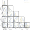 |
Fig. A.1. 1 and 2σ contours and the marginalized distributions of the halo parameters from the MCMC fitting (Sec. 4) for the f = 10 samples (blue: for supercluster members, yellow: for isolated clusters). |
All Tables
All Figures
|
Fig. 1. Comparison of the properties of the two subsamples before trimming: blue for supercluster members and yellow for isolated clusters. The red rectangle in the left panel defines the M − z space where we select the subsamples for further selection (trimming). The histograms in the right panel show the distribution of redshift, mass, and exposure time of the two subsamples before the trimming process. |
| In the text | |
|
Fig. 2. Comparison of the properties of the two subsamples after trimming. The histograms show the distribution of redshift, mass, and exposure time, from left to right. Supercluster members and isolated clusters are plotted in blue and yellow, respectively. |
| In the text | |
|
Fig. 3. Median electron density profiles. In the upper panel, the results for supercluster members and isolated clusters are plotted in blue and yellow, respectively. The uncertainties of the two profiles are almost negligible due to the large number of clusters in each sample. The difference in gas mass concentration between the two samples is almost invisible. In the lower panel, we plot the results for the two control samples, which are selected by randomly dividing the cluster sample into two. |
| In the text | |
|
Fig. 4. Confidence level of the excess in gas mass concentration, cgas. The histogram shows the distribution of δcgas defined as cgas, S1/cgas, S2 − 1 when randomly dividing the clusters into two subsamples (S1 and S2) and repeating 1000 times. The dashed lines indicate the δcgas when the clusters are divided into supercluster members and isolated clusters. The results are shown for different overdensity ratios in the identification of superclusters. The shaded area represents 1σ uncertainty. The cyan and purple lines correspond to 1.6σ for f = 10 and 2.0σ for f = 50, respectively. |
| In the text | |
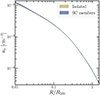 |
Fig. 5. Same as the left panel of Fig. 3 but for the supercluster sample of f = 50. |
| In the text | |
|
Fig. 6. Summary of the results for δcgas obtained in this work for different choices of overdensity ratio f in supercluster identification, cluster mass proxy, and mass range. The results for f = 10 and f = 50 are plotted in cyan and purple, respectively, to show the increasing trend in δcgas with f. The two measurements for the total mass concentration obtained from weak-lensing analysis, |
| In the text | |
|
Fig. 7. Measured weak-lensing ΔΣ profiles (top), the cross components for a null test (middle), and the boost factors (bottom) for the f = 10 sample (left) and the f = 50 sample (right). The supercluster members are plotted in blue and the isolated clusters in yellow. The shaded regions represent the 68% confidence best-fit interval, while the dashed lines correspond to the best-fit models. |
| In the text | |
|
Fig. 8. Same as the left panel of Fig. 3 but without considering the difference in exposure time of the supercluster members and isolated clusters. The y-axis is rescaled by the radius to reduce the dynamic range of the plot and improve the visibility of the difference between the two samples. The median electron density profile of supercluster members (blue) shows an apparently lower concentration than that of the isolated clusters (yellow). However, this trend should not be simply interpreted as the signal of HAB. It is mostly caused by the fact that supercluster members are located in areas with higher survey depths, where low-concentration clusters have a higher probability of being detected. This plot demonstrates the importance of correcting for selection effects in the analysis of HAB. |
| In the text | |
|
Fig. A.1. 1 and 2σ contours and the marginalized distributions of the halo parameters from the MCMC fitting (Sec. 4) for the f = 10 samples (blue: for supercluster members, yellow: for isolated clusters). |
| In the text | |
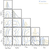 |
Fig. A.2. Same as Fig. A.1 but for the f = 50 sample. |
| In the text | |
Current usage metrics show cumulative count of Article Views (full-text article views including HTML views, PDF and ePub downloads, according to the available data) and Abstracts Views on Vision4Press platform.
Data correspond to usage on the plateform after 2015. The current usage metrics is available 48-96 hours after online publication and is updated daily on week days.
Initial download of the metrics may take a while.