| Issue |
A&A
Volume 677, September 2023
|
|
|---|---|---|
| Article Number | A12 | |
| Number of page(s) | 29 | |
| Section | Planets and planetary systems | |
| DOI | https://doi.org/10.1051/0004-6361/202346370 | |
| Published online | 28 August 2023 | |
TOI-1416: A system with a super-Earth planet with a 1.07 d period★
1
Instituto de Astrofísica de Canarias,
38205
La Laguna, Tenerife, Spain
e-mail: This email address is being protected from spambots. You need JavaScript enabled to view it.
2
Departamento de Astrofisica, Universidad de La Laguna,
38206
La Laguna, Tenerife, Spain
3
Department of Space, Earth and Environment, Chalmers University of Technology, Onsala Space Observatory,
439 92
Onsala, Sweden
4
Institute of Astronomy, Faculty of Physics, Astronomy and Informatics, Nicolaus Copernicus University,
Grudziądzka 5,
87–100
Toruń, Poland
5
NASA Exoplanet Science Institute,
770 South Wilson Ave.,
Pasadena, CA
91125, USA
6
Division of Geological and Planetary Sciences, California Institute of Technology,
1200 E California Boulevard,
Pasadena, CA
91125, USA
7
Department of Astronomy and Astrophysics, University of California,
Santa Cruz, CA
95064, USA
8
Institut für Physik, Karl-Franzens Universität Graz,
Universitätsplatz 5/II, NAWI Graz,
8010
Graz, Austria
9
Department of Physics and Kavli Institute for Astrophysics and Space Research, Massachusetts Institute of Technology,
Cambridge, MA
02139, USA
10
Deutsches Zentrum für Luft- und Raumfahrt, Institut für Planetenforschung,
12489
Berlin,
Rutherfordstrasse 2, Germany
11
Department of Physics and Astronomy, George Mason University,
4400 University Drive,
Fairfax, VA
22030, USA
12
Space Telescope Science Institute,
3700 San Martin Drive,
Baltimore, MD
21218, USA
13
Mullard Space Science Laboratory, University College London,
Holmbury St. Mary, Dorking,
Surrey,
RH5 6NT, UK
14
Thüringer Landessternwarte Tautenburg,
Sternwarte 5,
07778
Tautenburg, Germany
15
McDonald Observatory and Center for Planetary Systems Habitability, The University of Texas,
Austin, TX
78730, USA
16
Center for Astrophysics | Harvard & Smithsonian,
60 Garden Street,
Cambridge, MA
02138, USA
17
Leiden Observatory, Leiden University,
2333 CA
Leiden, The Netherlands
18
NASA Ames Research Center,
Moffett Field, CA
94035, USA
19
Astronomical Institute, Czech Academy of Sciences,
Fričova 298,
25165,
Ondřejov, Czech Republic
20
Rheinisches Institut für Umweltforschung an der Universität zu Köln,
Aachener Strasse 209,
50931
Köln, Germany
21
Komaba Institute for Science, The University of Tokyo,
3-8-1 Komaba, Meguro,
Tokyo
153-8902, Japan
22
Dipartimento di Fisica, Università degli Studi di Torino,
Torino, Italy
23
Astrobiology Center,
2-21-1 Osawa, Mitaka,
Tokyo
181-8588, Japan
24
Astronomy Department and Van Vleck Observatory, Wesleyan University,
Middletown, CT
06459, USA
25
Department of Earth, Atmospheric and Planetary Sciences, Massachusetts Institute of Technology,
Cambridge, MA
02139, USA
26
Department of Aeronautics and Astronautics, Massachusetts Institute of Technology,
77 Massachusetts Avenue,
Cambridge, MA
02139, USA
27
Department of Astronomy & Astrophysics, University of Chicago,
Chicago, IL
60637, USA
28
Department of Physics & Astronomy, University of California Los Angeles,
Los Angeles, CA
90095, USA
29
Okayama Observatory, Kyoto University,
3037-5 Honjo, Kamogatacho, Asakuchi,
Okayama
719-0232, Japan
30
Department of Multi-Disciplinary Sciences, Graduate School of Arts and Sciences, The University of Tokyo,
3-8-1 Komaba, Meguro,
Tokyo
153-8902, Japan
31
Département d’Astrophysique, IRFU/DRF/CEA Saclay,
L’Orme des Merisiers, bat. 709,
91191
Gif-sur-Yvette Cedex, France
32
Department of Astrophysical Sciences, Princeton University,
Princeton, NJ
08544, USA
33
University of California at Berkeley,
501 Campbell Hall,
Berkeley, CA
94720, USA
34
Observatori Astronòmic Albanyà,
Camí de Bassegoda s/n, Albanyà
17733,
Girona, Spain
35
Department of Physics, Engineering and Astronomy, Stephen F. Austin State University,
1936 North St,
Nacogdoches, TX
75962, USA
36
National Astronomical Observatory of Japan,
2-21-1 Osawa, Mitaka,
Tokyo
181-8588, Japan
37
Department of Astronomical Science, School of Physical Sciences, The Graduate University for Advanced Studies (SOKENDAI),
2-21-1, Osawa, Mitaka,
Tokyo,
181-8588, Japan
38
Centre for Astrophysics, University of Southern Queensland,
Toowoomba, QLD, Australia
Received:
10
March
2023
Accepted:
10
May
2023
Abstract
TOI-1416 (BD+42 2504, HIP 70705) is a V =10 late G- or early K-type dwarf star. TESS detected transits in its Sectors 16, 23, and 50 with a depth of about 455 ppm and a period of 1.07 days. Radial velocities (RVs) confirm the presence of the transiting planet TOI-1416 b, which has a mass of 3.48 ± 0.47 M⊕ and a radius of 1.62 ± 0.08 R⊕, implying a slightly sub-Earth density of 4.50−0.83+0.99 g cm−3. The RV data also further indicate a tentative planet, c, with a period of 27.4 or 29.5 days, whose nature cannot be verified due to strong suspicions of contamination by a signal related to the Moon’s synodic period of 29.53 days. The nearly ultra-short-period planet TOI-1416 b is a typical representative of a short-period and hot (Teq ≈ 1570 K) super-Earth-like planet. A planet model of an interior of molten magma containing a significant fraction of dissolved water provides a plausible explanation for its composition, and its atmosphere could be suitable for transmission spectroscopy with JWST. The position of TOI-1416 b within the radius-period distribution corroborates the idea that planets with periods of less than one day do not form any special group. It instead implies that ultra-short-period planets belong to a continuous distribution of super-Earth-like planets with periods ranging from the shortest known ones up to ≈30 days; their period-radius distribution is delimited against larger radii by the Neptune Desert and by the period-radius valley that separates super-Earths from sub-Neptune planets. In the abundance of small, short-periodic planets, a notable plateau has emerged between periods of 0.6–1.4 days, which is compatible with the low-eccentricity formation channel. For the Neptune Desert, its lower limits required a revision due to the increasing population of short-period planets; for periods shorter then 2 days, we establish a radius of 1.6 R⊕ and a mass of 0.028 Mjup (corresponding to 8.9 M⊕) as the desert’s lower limits. We also provide corresponding limits to the Neptune Desert against the planets’ insolation and effective temperatures.
Key words: planets and satellites: individual: TOI-1416 b / planets and satellites: detection / planets and satellites: terrestrial planets / planetary systems / planets and satellites: composition / techniques: radial velocities
Data are only available at the CDS via anonymous ftp to cdsarc.cds.unistra.fr (130.79.128.5) or via https://cdsarc.cds.unistra.fr/viz-bin/cat/J/A+A/677/A12
© The Authors 2023
 Open Access article, published by EDP Sciences, under the terms of the Creative Commons Attribution License (https://creativecommons.org/licenses/by/4.0), which permits unrestricted use, distribution, and reproduction in any medium, provided the original work is properly cited.
This article is published in open access under the Subscribe to Open model. This email address is being protected from spambots. You need JavaScript enabled to view it. to support open access publication.
1 Introduction
Small exoplanets (R ≲ 2.5 R⊕) currently constitute the most numerous group of known exoplanets. Their population properties were first studied by Sanchis-Ojeda et al. (2014), who identified several tens of planets (or planet candidates) with periods of less than 1 day in data from the Kepler mission (Borucki et al. 2010), calling them ultra-short-period planets (USPs). Nearly all of these planets were smaller than 2R_Earth, and a preference for the presence of additional planets with periods of up to 50 days was identified. The upper limit choice of 1 day for USPs – besides being a convenient number – was due to the lower period limit of the Kepler planet detection pipeline (Jenkins et al. 2010), which had missed these planets, and not due to any physical limit. However, the term “USP” with that period limit has remained with the community, and currently there are 126 such planets known, though there are only 34 for which both masses and radii have been determined1. For overviews of this population and theories regarding their development, we refer to Winn et al. (2018), Murgas et al. (2022), and references therein.
In this work, we describe the detection of a planet around the late G or early K star TOI-1416 (see Table 1), which has a period of 1.069 days, just outside of the conventional definition of USPs, and we place it in context with the population composed of USPs and planets with slightly longer orbits. TOI-1416 b was found in light curves from the Transiting Exoplanet Survey Satellite (TESS; Ricker et al. 2015), whose all-sky transit survey with relatively short coverages is well suited for the detection of short-period planets. The TESS observations and their processing is described in Sect. 2. A ground-based follow-up campaign involving imaging and radial velocity (RV) observations is described in Sect. 3. The analysis of the data via stellar modeling (Sect. 4) and planet system modeling (Sect. 5) led to the detection of a potential second planet, TOI-1416 c, with a period of 27–29 days.
Strong doubts remain, however, about the origin of its potential RV signal, which may instead be the product of Moon-reflected solar light (details are given in Appendix A). The implications of these findings, in particular with regard to the planet’s composition and its placement relative to the short-period planet population, are provided in Sect. 6, and conclusions are given in Sect. 7.
Parameters of TOI-1416 from catalogs.
2 Photometry by TESS
TESS observed TOI-1416 in its Sectors 16, 23, and 50, with more detailed information given in Table 2. Planet b was initially detected in S16 as a TESS object of interest (TOI) by the TESS Science Processing Operations Center (SPOC) pipeline (Jenkins et al. 2016), as TOI 1416.01. A subsequent analysis of the combined S16, S23 and S50 data by the same pipeline specified a transit-like signal2 with a period of P = 1.06975[1] days and an amplitude of 391.5± 24.0 ppm, indicating a candidate for a small planet of ≈1.6 R⊕. The difference imaging test (Twicken et al. 2018) also revealed that the origin of the transit is within 2.47″ of the location of the target.
For our own transit detection analysis, we used the DST (Détection Spécialisée de Transits; Cabrera et al. 2012) and transit least square (TLS) algorithms (Hippke & Heller 2019) to search for transit signals in the existing TESS data and found a signal with period of P = 1.07 days, which was consistent with the detection reported by SPOC. We then masked the transits at 1.07 days and searched for further signals in the data set but found no detections of additional transiting planet candidates. This process was repeated later with a focus on signals with periods of ≈10 days and 27–30 days, corresponding to peaks in RV periodograms reported in Sect. 5 of this work, but again to no avail.
For all further analysis of light curves, we used the presearch data conditioned simple aperture photometry (PDCSAP) fluxes (Stumpe et al. 2012, 2014; Smith et al. 2012, 2020b) available at MAST. Flux points in which some quality flags are raised3 were removed. Also, the fluxes were normalized to an average flux of 1 in each sector independently. This light curve was used for the fit using Gaussian processes (GPs) with pyaneti described in Sect. 5.2.
The field around TOI-1416 is moderately crowded and the TIC indicates a contamination ratio4 of cTIC = 0.193. Very similar values for contamination are also indicated by the CROWDSAP keyword5 in the headers of the SPOC light curves from S16 and S23, whereas the S50 light curves indicates only very minor contamination. PDCSAP fluxes are in principle corrected against contamination (Smith et al. 2020a), but not indications about the uncertainty of cTIC (or CROWDSAP) are given. We hence evaluated the impact that an error in cTIC (or in the corresponding CROWDSAP values) might have onto the final system parameters reported in Tables 7 and 8. The impact of an error of cTIC was however found to be negligible as long as cTIC is correct within ≈25%. In consequence, we did not propagate this uncertainty into the finally given parameter errors.
Individual transits of TOI-1416 b have a signal-to-noise ratio (S/N) of ≈3.6 and they are too shallow to be individually detectable in the light curve. For the preparation of the light curve to be used in transit fits with the Universal Transit Modeller/Fitter (UTM/UFIT6; described in Appendix C), we extracted short sections between orbital phases of ±0.125 around the transit center of planet b (using initially the ephemeris provided by SPOC, and then improved ones from our own transit fits) and performed linear fits across the off-transit sections on both sides of each transit. The fluxes were then divided by that fit, which leads to an off-transit flux that is normalized to 1. Only transits that were fully covered by TESS have been included in the final light curve (see Table 2 for the number of transits in each sector). The phase-folded light curve containing 48 transits is shown in Fig. 1. With the transit ephemeris that was finally adopted and which is given in Table 7, it shows a transit-shape that is much better defined – with steeper in- and egress – than one produced by a folding with the original period indicated by SPOC. The standard deviation (or rms noise) of the unbinned off-eclipse data is 765 ppm, and the noise of a smoothed and binned version of the phased light curve, with a temporal resolution similar to TESS’s 2-min cadence (green crosses in Fig. 1) is 86 ppm, while the depth of the transits is ≈455 ppm and the S/N of the phased transit is ≈25.
Table 2 indicates also transit epochs for each sector individually, corresponding to a transit near the middle of each sector’s data. These were derived using UTM/UFIT with a setup that was identical to the transit fit on the combined (S16 to S50) light curve described in Appendix C. Against the adopted ephemeris from Table 7, a diagram of observed minus calculated (O – C) times (Fig. 2) shows no relevant deviation that might indicate the presence of transit timing variations (TTVs).
TESS observations of TOI-1416.
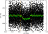 |
Fig. 1 Phased light curve around the transits of TOI-1416 b. Black crosses represent the TESS light curve, after phasing by the planet’s period against the adopted ephemeris and the correction against gradients in the off-transit sections, as described in Sect. 2. Green crosses represent the same curve after a box-car smoothing over 100 phased data points and posterior binning over 50 points. We note that the average time increment between the binned points is 126 seconds, which is very similar to the 120 s temporal resolution of TESS light curves. The red curve is the transit model generated with UTM/UFIT, described in Appendix C. The vertical dashed orange lines indicate the limits between the on-transit and off-transit sections. |
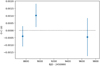 |
Fig. 2 O-C diagram of the transit epochs of TESS Sectors 16, 23, and 50, against the adopted ephemeris (dotted black line). |
RV observations of TOI-1416.
3 Ground-based follow-up
3.1 High-resolution spectroscopy
High-resolution spectroscopic observations of TOI-1416 were obtained by several instruments, described in more detail in the following sections, with an overview on the observations given in Table 3. Figure 3 shows a time series of all the RVs that have been collected. Corresponding tables with the RVs from each instrument and – if available – spectral indices can be found at the CDS.
3.1.1 3.5 m Calar Alto/CARMENES
We started the RV follow-up of TOI-1416 using the CARMENES instrument mounted on the 3.5 m telescope at Calar Alto Observatory, Almería, Spain, under the observing programs F19-3.5-014 and F20-3.5-011 (PI Nowak), setting the exposure times to 1800 s. The CARMENES spectrograph has two arms (Quirrenbach et al. 2014, 2018): the visible (VIS) arm covers the spectral range 0.52–0.96 µm and a near-infrared arm covers the spectral range 0.96–1.71 µm. Due to the S/N that was obtained, only the VIS channel observations could be used to derive useful RV measurements. All observations were taken with exposure times of 1800 s, resulting in a S/N per pixel (at 4635.7 nm in the VIS spectra) in the range of 42 to 113. CARMENES performance, data reduction and wavelength calibration are described in Trifonov et al. (2018) and Kaminski et al. (2018). Relative RV values, chromatic index (CRX), differential line width (dLW), and Ha index values were obtained using serval7 (Zechmeister et al. 2018). For each spectrum, we also computed the cross-correlation function (CCF) and its full width half maximum (FWHM), contrast and bisector velocity span, following Lafarga et al. (2020). The RV measurements were corrected for barycentric motion, secular acceleration and nightly zero points.
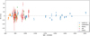 |
Fig. 3 Relative RVs of TOI-1416 from all contributing instruments. Each instrument’s set of RVs was offset separately to an average of zero. |
3.1.2 TNG/HARPS-N
A total of 96 spectra over three observing seasons were collected with the HARPS-N spectrograph with R ≈ 115 000 (Cosentino et al. 2012), mounted at the 3.58 m Telescopio Nazionale Galileo (TNG) at the Roque de los Muchachos Observatory in La Palma, Spain. The exposure times were 636–2700 s, based on weather conditions and scheduling constraints, leading to a S/N per pixel (at 5500 Å) of 48–138. The spectra were extracted using the HARPS-N DRS pipeline version 3.7 (Cosentino et al. 2014). Doppler measurements and spectral activity indicators (CCF_FWHM, CCF_CTR, BVS, and the Mount Wilson S-index) were measured using the DRS and the YABI tool8, by cross-correlating the extracted spectra with a K5 mask (Baranne et al. 1996). Furthermore, we used serval to measure relative RVs, chromatic RV index (CRX), dLW, and the Hα index, as defined in Zechmeister et al. (2018). While both DRS and serval derive very similar RVs (see also Fig. F.1), we adopted those from serval for further analysis, due to issues with DRS in those exposures that were terminated prematurely. The table of HARPS-N measurements available at the CDS contains the 96 RVs from both pipelines, together with all activity indicators extracted by either pipeline (indicated by suffixes _drs or _srv), in the following columns:
For most indicators, a column with the errors is also provided, not shown in above list.
| bjd_tdb | – | BJD_TDB |
| rvs_srv | – | Barycentric corrected relative RV (against a zero average) |
| rvs_drs | – | Barycentric corrected absolute RV |
| ccf_bis_drs | – | Bisector Inverse Slope (BIS) measured from Cross-Correlation Functions (CCFs) |
| ccf_fwhm_drs | – | Full Width at Half Maximum of CCF |
| ccf_ctr_drs | – | CCF contrast |
| smw_drs | – | Mont-Wilson S-index |
| log_rhk_drs | – | Log RHK |
| crx_srv | – | Chromatic RV index (CRX) |
| dlw_srv | – | Differential line width (dLW) |
| halpha_srv | – | H-alpha index |
| nad1_srv | – | Sodium Na D1 index |
| nad2_srv | – | Sodium Na D2 index |
| snr_5 50nm_drs | – | S/N at spectral order 46 (~5 50 nm) |
| expt | – | exposure time from FITS header |
3.1.3 IRTF/iSHELL
A total of 11 observations of TOI-1416 were obtained in as many nights with the iSHELL instrument at the NASA InfraRed Telescope Facility (IRTF; Rayner et al. 2022) atop Mauna Kea, Hawaii, USA, using its Kgas’ mode, which covers the wavelengths 2.17–2.47 µm. The exposure times were always set to 300 s, and exposures were repeated anywhere from 4 to 16 times consecutively per night, in order to obtain an S/N per spectral pixel of ≈120, though the actual results varied from 85 to 186 due to variable seeing and atmospheric transparency conditions. A methane isotopologue (13CH4) gas cell is used in the instrument (Cale et al. 2019) to constrain the line-spread function and to provide a common reference for the optical path wavelength. Along with each observation, a set of five 15-s flat-field images was also collected, with the gas cell removed for data reduction purposes, in order to mitigate flexure-dependent and time-variable fringing present in the spectra. The 11 RVs included in the electronic tables at the CDS are nightly averaged values from the individual exposures.
3.1.4 Keck/HIRES and Lick Observatory APF
The High Resolution Echelle Spectrometer (HIRES) at the 10m Keck Observatory (Vogt et al. 1994) was used to obtain 12 high-resolution spectra of TOI-1416, and the Automatic Planet Finder (APF) at Lick Observatory (Vogt et al. 2014) was used to obtain 52 high-resolution spectra. Each exposure of TOI-1416 was about 500 s on HIRES and 1200 s on APF. We also obtained an iodine-free spectrum on HIRES as the template for the RV extraction for both the HIRES and APF observations. The HIRES RVs were collected using the telescope setup, instrument setup, and analysis pipeline described in Howard et al. (2010). The APF RVs were collected using a 1″ decker and analyzed with the standard California Planet Search pipeline (Fulton et al. 2015).
3.2 Ground-based imaging and time-series photometry
The TESS pixel scale is ≈21″ per pixel and its photometric apertures typically extend out to roughly 1′, generally causing multiple stars to blend in the TESS aperture. Attempting to determine the true source of our detection in the TESS data, we conducted ground-based imaging and photometric time-series observations of the field around TOI-1416 as part of the TESS Follow-up Observing Program9 (TFOP) Sub Group 3 (High-resolution Imaging) and Sub Group 1 (Seeing limited Photometry; Collins 2019).
3.2.1 High-resolution imaging at Palomar Observatory
As part of our standard process for validating transiting exoplanets, and in order to assess the possible contamination by bound or unbound companions onto the derived planetary radii (Ciardi et al. 2015), we observed TOI-1416 with infrared high-resolution adaptive optics (AO) imaging at Palomar Observatory. The Palomar Observatory observations were made with the PHARO instrument (Hayward et al. 2001) behind the natural guide star AO system P3K (Dekany et al. 2013) on 2020-01-08 UT in a standard 5-point quincunx dither pattern with steps of 5″. Each dither position was observed three times, offset in position from each other by 0.5″ for a total of 15 frames. The camera was in the narrow-angle mode with a full field of view of ≈25″ and a pixel scale of approximately 0.025″ per pixel. Observations were made in the narrow-band Br − y filter (λo = 2.1686; Δλ = 0.0326 µm) with an integration time of 5.6 s per frame (118 s total).
The AO data were processed and analyzed with a custom set of tools written in IDL. The science frames were flat-fielded and sky-subtracted. The flat fields were generated from a median average of dark subtracted flats taken on-sky and then normalized to unity. The sky frames were generated from the median average of the 15 dithered science frames; each science image was then sky-subtracted and flat-fielded. The reduced science frames were combined into a single combined image using an intra-pixel interpolation that conserves flux, shifts the individual dithered frames by the appropriate fractional pixels, and median-coadds the frames (Fig. 4). The final resolution of the combined dither was determined from the FWHM of the point spread function, as 0.11″ (Fig. 5).
No sources, other than the primary target, were detected. The sensitivities of the final combined AO image were determined by injecting simulated sources azimuthally around the primary target every 45° at separations of integer multiples of the central source’s FWHM (Furlan et al. 2017; Lund et al., in prep.). The brightness of each injected source was scaled until standard aperture photometry detected it with 5σ significance. The resulting brightness of the injected sources relative to the target sets the contrast limits at that injection location. The final 5σ limit at each separation was determined from the average of all of the determined limits at that separation and the uncertainty on the limit was set by the rms dispersion of the azimuthal slices at a given radial distance. The sensitivity curve is shown in Fig. 5 along with an image zoomed around the target, showing no other companion stars. We also note that an interrogation of Gaia Early Data Release 3 (EDR3) showed the most nearby star at 23″ W of the target and 11.4 mag fainter, whereas as the second closest one is 51″ NE and 9.5 mag fainter; due to their faintness, neither of these stars can be responsible for the transits on TOI-1416.
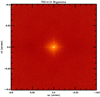 |
Fig. 4 Full field of view image of the final combined dither pattern for the Palomar AO imaging. |
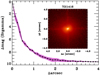 |
Fig. 5 Companion sensitivity for the Palomar AO imaging. The black points represent the 5σ limits and are separated in steps of 1 FWHM (≈0.1″); the purple zone represents the azimuthal dispersion (lσ) of the contrast determinations (see the main text). The inset image is of the primary target and shows no additional companions within 3″ of the target. |
3.2.2 Time-series photometry with MUSCAT2
TOI-1416 was observed with the MUSCAT2 multi-colour imager (Narita et al. 2019) mounted at the 1.5 m Telescopio Carlos Sanchez at Teide Observatory, Tenerife, Spain, on several dates: between 2020-01-17 03:42 and 06:12 UT covering a full transit of planet b; between 2021-05-03 22:19 and 2021-05-04 02:09 UT with a partial transit (ingress) and between 2022-04-20 20:45 and 2022-04-21 00:07 UT for a full transit. The raw data were reduced by the MuSCAT2 pipeline (Parviainen et al. 2019) which performs standard image calibration with aperture photometry and is capable of modeling the instrumental systematics present in the data while simultaneously fitting a transit model to the light curve. Due to the target’s brightness, only short exposure times could be used. Given the noise present, no evidence for a transit could be found on the target. There are 77 sources listed in Gaia Data Release (DR) 3 in a radius of 2.5′ around the target, of which 7 have a brightness large enough that they could potentially be an eclipsing binary that mimics the transit observed by TESS. Of these, however, only the star TIC 158025007, which is the brightest nearby contaminant and about 1.5′ south of the target, could be excluded with certainty as a source for a false alarm.
3.2.3 Time-series photometry with LCOGT
We observed full predicted transit windows of TOI-1416 b on 2020-05-21 UT and 2021-03-08 UT using the Las Cumbres Observatory Global Telescope (LCOGT; Brown et al. 2013) 1.0m network node at McDonald Observatory. The 1 m telescopes are equipped with 4096 × 4096 pixel SINISTRO cameras having an image scale of 0.389″ per pixel, resulting in a 26′ × 26′ field of view. The images were calibrated by the standard LCOGT BANZAI pipeline (McCully et al. 2018) and differential photometric data were extracted using AstroImageJ (Collins et al. 2017).
We extracted light curves from the 2020-05-21 UT data for all six known Gaia DR3 and TICv8 neighboring stars within 2.5′ of TOI-1416 that are bright enough to produce a detection by TESS. We thus checked all stars down to 8.4 mag fainter than TOI-1416 (i.e., down to 17.5 mag in the TESS band). We calculated the rms of each of the six nearby stars’ light curves (binned in 5 min bins) and find that the LCOGT light curve rms values are smaller by at least a factor of 5 compared to the expected NEB (Nearby Eclipsing Binary) depth in each respective star. We then visually inspected the neighboring star light curves to ensure no obvious deep eclipse-like signal. We therefore rule out NEBs as the cause of the TOI-1416 b detection in the TESS data.
For the second observation on 2021-03-08 UT, we defo-cused the telescope to improve photometric precision and attempted to detect the shallow TOI-1416 b event on target. As shown in Fig. 6, we find a likely transit detection centered at 2459281.827 ± 0.005 BJDTDB with a depth of 350 ± 100 ppm. The difference between the Bayesian information criterion (BIC) of the transit model shown and a model without any transit was a Δ-BIC of −43 in favor of the transit model.
4 Stellar modeling
4.1 Spectral analysis
We started our analysis of the host star by first deriving the stellar effective temperature Teff, the stellar radius R★ and the abundance of iron relative to hydrogen [Fe/H], with the empirical SpecMatch-Emp code (Yee et al. 2017). We modeled our co-added high-resolution (R = 115 000) HARPS-N spectra with a S/N of 346 at 6100 Å. This software characterizes stars from their optical spectra and compares observations to a dense spectral library of well-characterized FGKM stars observed with Keck/HIRES.
In addition to SpecMatch-Emp, we analyzed the co-added HARPS-N spectra with version 5.22 of the spectral analysis package Spectroscopy Made Easy (SME10; Valenti & Piskunov 1996; Piskunov & Valenti 2017). This software is fitting observed spectra to calculated synthetic stellar spectra for a given set of parameters. We chose the Atlas12 (Kurucz 2013) atmosphere grids, and retrieved the atomic and molecular line data from the Vienna Atomic Line Database (VALD11; Ryabchikova et al. 2015) to synthesize the spectra. We modeled Teff from the line wings of the hydrogen 6563 Å line, and the surface gravity log g from the calcium triplet at 6102, 6122 and 6162 Å, and from the 6439 Å line. We fitted the iron and calcium abundances, the projected stellar rotational velocity V sin i★ and the macroturbulent velocity Vmac from unblended lines between 6000 and 6600 Å. The sodium abundance was fitted from spectral lines between 5600 and 6200 Å. We found similar abundances of iron, calcium and sodium, and determined V sin i★ = 2.0 ± 0.7 km s−1 and Vmac = 1.5 ± 1.0 km s−1. To check and further refine our model, we used the Na I doublet at 5888 and 5895 Å. The resulting model suggests that TOI-1416 is a an early K dwarf star.
Results from both models are listed in Table 4 and are in good agreement within the uncertainties. They also agree well with the corresponding values from Gaia DR2 and from the TESS Input Catalogue (TIC; Stassun et al. 2018, 2019).
The metallicity and kinematics of TOI-1416 point to a membership in the galactic thin disk. Following the precepts of Reddy et al. (2006), we obtain a thin-disk membership probability of 0.975 ± 0.012.
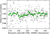 |
Fig. 6 Time series of a predicted transit of TOI-1416 b on March 08, 2021 UT, observed by the LCOGT. The gray dots are the unbinned differential photometry (no detrending applied), and the green dots show the data in 10-min bins. The green line is a transit-model fit to the data using priors from the Data Validation Report mentioned in Sect. 2, except for the epoch and the size of the planet, which were unconstrained parameters. |
4.2 Stellar mass, radius, and age
To obtain an independent estimate of the stellar radius, we analyzed the spectral energy distribution (SED) of TOI-1416 with the python code ARIADNE (Vines & Jenkins 2022). This software fits broadband photometry to the Phoenix v2 (Husser et al. 2013), BtSettl (Allard et al. 2012), Castelli & Kurucz (2003), and Kurucz (1993) atmospheric model grids for stars with Teff > 4000 K, convolved with various filter response functions. For TOI-1416, we utilized data in the bandpasses G, GBP and GRP from Gaia EDR3, W1 and W2 from WISE, JHKS magnitudes from 2MASS, and the Johnson B and V magnitudes from APASS DR9 (AAVSO Photometric All-Sky Survey; Henden et al. 2016). By interpolating the Teff, log ɡ★, and [Fe/H] model grids, SED models were produced where distance, extinction (AV), and stellar radius are treated as free parameters. The Gaia EDR3 parallax was used to obtain the distance (Table 1), while priors for Teff, log ɡ★ and [Fe/H] were taken from SME. We used flat priors for R★ between 0.05 and 20 R⊙, and for AV between zero and the maximum line-of-sight value from the dust maps of Schlegel et al. (1998). Each SED model was integrated to get the bolometric flux, which, together with Teff and the Gaia EDR3 parallax, gives the stellar radius for each fitted model. The weighted average of each parameter is computed based on the relative probabilities of the models, and the final value of the stellar radius is computed with Bayesian model averaging. The Phoenix v2 model grid that has the highest probability was used to calculate the synthetic photometry. The model is shown in Fig. 7 along with the fitted bands.
In addition to the above modeling we used the python code isochrones (Morton 2015) to obtain a homogeneous model of TOI-1416. This code is fitting stellar parameters with a Markov chain Monte Carlo (MCMC) fitting tool and the MIST (Choi et al. 2016) stellar evolution tracks. We used the same bands and priors as in the ARIADNE model. We find AV = 0.05 ± 0.04 mag, and a bolometric luminosity of 0.34 ± 0.03 L⊙. The resulting stellar properties are in very good agreement with the values found by the above models.
As a comparison, we used the Param 1.5 on-line tool (da Silva et al. 2006; Rodrigues et al. 2014, 2017) with the PARSEC isochrones (Bressan et al. 2012) and the same bands and priors as in the above models. And finally, we used the empirical calibration equations of Torres (2010) to compute stellar mass and radius from Teff, log ɡ, and [Fe/] from SME.
All results are in excellent agreement. The stellar masses, radii and corresponding bulk densities are listed in Table 5 together with the radius from Gaia DR2 and values from the TIC. The adopted values, which were also used in the joint modeling of the RVs and light curves in Sect. 5.2, were derived by the adding of simulated probability distributions that are associated with each of the values from the different methods (the values from the TIC were not used for this), using two-sided Gaussian distributions with 1 million elements. Hence, each of the methods has been taken with equal weight. In the resultant distribution, the percentiles at 15.9, 50, and 84.1% where then used to quote the median and the ±1-sigma errors. The derived values for the temperature place TOI-1416 right at the border between spectral classes G and K, with a slight preference for spectral class G9V, due to the notable Ca H& K lines (Fig. 8), which are a defining feature of the class G (Cannon & Pickering 1901, p. 158). The mean  index of log(
 ) = −4.86 ± 0.03 from the 96 HARPS-N spectra indicates however only very moderate chromospheric activity. This activity implies also an age in the range of 4–7 Gyr, based on the activity-age relation by Mamajek & Hillenbrand (2008). Ages from the aforementioned isochrone analyses are not very well constrained but indicate a similar evolutionary phase, with MIST isochrones indicating an age of
  Gyr and Param 1.5 one of
  Gyr, which in either case rules out TOI-1416 as a very young system. With TOI-1416 being a likely thin-disk member and age estimates for the local thin disk of 6.8–7.0 Gyr (Kilic et al. 2017), the age of TOI-1416 is most likely close to that value.
In Appendix A, we also present an analysis of the stellar rotation based on the TESS light curves, leading to Prot = 17.6 days, which is also compatible with a rotation period of  days from the star’s V sin i. Such a rotation leads, however, to a gyrochronological age of 1–2 Gyr (see Appendix A for several rotation-based age estimations). This apparently young age might however be a consequence from a delay in the star’s age-related spin-down, due to angular momentum transfer from the planet to the host star (Hut 1980), given that planet b’s orbital period is much shorter than the star’s rotation period. The work by Ahuir et al. (2021) indicates that a planet with the mass and orbital period of TOI-1416 b might have a moderate effect on the star’s rotation through magnetic interactions (Strugarek 2016), and hence invalidate its gyrochronological age. However, more detailed studies that also include mass-loss scenarios for the planet (e.g., Attia et al. 2021) would be needed for a better estimate of the planet’s influence onto the evolution of the stellar rotation, which might then permit a correction of its gyrochronological age.
Spectroscopic parameters for TOI-1416 derived with SME and SpecMatch-Emp and comparison values from Gaia and the TIC.
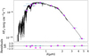 |
Fig. 7 SED of TOI-1416. The best fitting model from the Phoenix v2 grids is shown in black. The observed photometry is marked with cyan circles, and the synthetic photometry with magenta diamonds. The horizontal bars of the observations indicate the effective widths of the passbands, while the vertical bars mark the 1 σ uncertainties. The lower panel shows the residuals normalized to the errors of the photometry, which causes the most precise photometry to display the largest scatter. |
Stellar masses and radii with corresponding mean densities of TOI-1416 derived with different models with priors from SME.
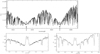 |
Fig. 8 Co-added HARPS-N spectrum of TOI-1416 in the range of the Ca H & K lines (arrows), with zoomed-in views (lower panels) around the Ca K (3933.66 Å) and Ca H (3968.47 Å) lines. |
5 Planet system modeling
In this section we first provide an analysis of the periodicities and activity indicators in the RV data, with a detailed evaluation of a potential contamination of RV signals by lunar light given in Appendix B. This is followed by a joint RV/transit fit using Gaussian Processes (GPs), in which several models with and without a second planet were evaluated. A fit to the RVs using the floating chunk offset (FCO) method (Hatzes et al. 2010; Hatzes 2014) provided a clear detection of the transiting planet b and is described in Appendix D. Also, a classical fitting (Bayesian but without GPs) to the transit light curve was performed with the UTM/UFIT package (Deeg 2014). These fits, which were also used in some other parts of this work, are described in Appendix C. The results from all methods are included in Table 7.
5.1 Periodicities in the RV data: Planetary signals or stellar activity?
Beyond the anticipated detection of RV signals from the P = 1.07 days transit-candidate found by TESS, the RV data may contain further signals that need a revision about their nature, be they one or more additional planet(s) in the system, or due to other sources. The RVs acquired with HARPS-N are the most precise ones (with the exception of data from HIRES, from which only 12 RV points were acquired) and also have the most consistent coverage by far (see also Table 3); our analysis will hence concentrate on these data. Tests that included RVs from other instruments showed in all cases a degradation in the detection of the 1.07 days signal. Data from the other instruments are however used in the evaluation of a potential contamination of the RV signals by the Moon, which is described in detail in Appendix B.
In Fig. 9, we show Bayesian generalized Lomb-Scargle (BGLS) periodograms (Mortier et al. 2015)12 of the HARPS-N RVs and of the more common activity indicators from the list in Sect. 3.1.2. The BGLS provides several improvements over the common Lomb–Scargle periodograms: it weights the data points by their errors; it is independent of the setting of the data’s zero point, and lastly, it provides a quantifiable probability of the relevance of the periodogram peaks. Figure 9 shows also the spectral window function (Roberts et al. 1987; Dawson & Fabrycky 2010), whose peaks indicate the likely presence of artifacts due to the temporal distribution of the observations. In the RV periodogram, a double peak with a highest probability at 29.5 days is of prominence, with a slightly lower peak (albeit by a factor of log p ≈ 10) at 27.4 days (see also Fig. B.1). Among the activity indicators, only the CRX has peak near ≈30 days, while the window function is rather flat in this region. We note that the period of the higher of the double-peak is very close to the lunar synodic period of 29.53 days. Appendix B provides a more detailed evaluation of this signal as a candidate for a second planet c.
A further signal is notable at ≈10 days, which corresponds to local maxima of most activity indicators. Hence, it is likely due to stellar activity13, albeit at a shorter period than the stellar rotation period of  days determined from V sin i★ and R★ or the 17.6 ± 2 days from the light curve analysis of Appendix A. The same goes for an RV peak at 138 days, with several activity indicators showing maxima at a slight larger period of ≈160 days, which we did not consider further. The periodicity of the transits of 1.07 days does not appear clearly in the BGLS periodogram, which instead shows a series of peaks around P≈ 1 day, with the highest and second highest ones at P = 1.035 days and P = 0. 967 day, respectively. These are clearly aliases of the 29.5 days signal due to a sample period of 1 day (Fig. 10), given by the aliasing equation falias = |freal + Nfsample| with N = ± 1, where the f are the frequencies of the alias signal, the real signal, and the sample frequency, respectively.
In a further evaluation, we use the framework provided by the online-tool Agatha14 (Feng et al. 2017). With this tool, in a first step a comparison between different models describing the data is performed. In this process, agatha evaluates moving average (MA) models of varying complexity to describe the RV’s red noise. These MA models are simplified GPs that only account for the correlation between previous data points and the current point, for which models with zero (corresponding to purely white noise), one, or more MA components are evaluated. We then used agatha to evaluate models with 0–2 MA components and with none, one, or several noise-proxies among the activity indicators. For the different MA models (with or without the presence of proxies) that were evaluated, agatha generated Bayes factors that account for the varying complexity of the models. In the case of our HARPS-N data, a one-component MA model without any noise proxies was indicated as the best model. This model was then also used by agatha to generate the Bayes factor periodogram (as defined by Feng et al. 2017) shown in Fig. 11. In this periodogram, the highest peak by a wide margin corresponds to the 1.07 days period of the transits. Beyond the peaks around P = 1 day, the next highest peak is again a signal near 29.5 days, identified previously with the BGLS periodogram and suspiciously close to the lunar synodic period.
Lastly, we generated correlations between the various activity indicators and the RVs, following the precepts of Díaz et al. (2018), which was based on prior work by Santos et al. (2014). Figure 12 shows no strong correlation between any of these indicators and the RVs, with a notable absence of any correlation between the RVs and the bisector inverse slope (in Fig. 12 labeled as ccf_bi s_drs). The only correlations worth mentioning are the weak ones of the RVs against the dLW, or against the CCF contrast, with correlation coefficients of −0.41 + 0.07 or 0.37 ± 0.07, respectively.
Considering the significant differences between periodograms generated by different methods (for further examples of strongly differing results among different periodograms, see Feng et al. 2017, their Figs. 1, 3, and 5), none of them should be taken to provide definite results. In any case, these periodograms suggest the presence of planet-like RV signals with periods of 1.07 and 29.5 (or potentially 27.5) days. The detailed evaluation about the 29.5 days signal being caused by the Moon, in Appendix B, is not fully conclusive but a strong chance remains that it is a residual from contamination by Moon light; hence at most it may be treated as a tentative planet. Further modeling of the data concentrates therefore on the short-period transiting planet b.
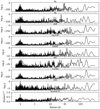 |
Fig. 9 BGLS periodograms of the HARPS-N observations, for the measured RVs and for several activity indicators. The vertical scale is given in units of the logarithm of the Bayesian probability of a signal with a given period, where the highest peak is normalized to log p = 0. The lowest panel shows the spectral window function of the sampled data. See also Figs. 10 and B.1 for zoomed-in views around the 1.07 days and 29.5 days periods of planet b and the candidate c, respectively. |
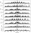 |
Fig. 10 Zoomed-in view of the BGLS periodogram of Fig. 9, around the 1.07 days period of the transiting planet, b, where only a minor peak is discernible in the RVs (top panel). The highest RV peaks at P = 1.035 days and P = 0.967 days are aliases of the 29.5 days signal over the sample period of the solar or the sidereal day. Their periods of 1.0 and 0.9973 days show up as the principal double peak in the window function (lowest panel). |
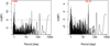 |
Fig. 11 Left panel: Bayes factor periodogram of the HARPS-N RVs generated by agatha (Feng et al. 2017), using one MA component. The vertical axis provides the probability of peaks being real, in terms of the logarithm of their Bayes factor (BF). The period of the highest peak is indicated, which corresponds to the period of the transits of TOI-1416 b. Right panel: Like the left panel, but after the removal of the 1.069 days signal, now showing a signal at 29.52 days as the highest one. |
5.2 Joint RV and light curve modeling
“Classical” Keplerian RV fits that assume white noise in the jitter of the RV values performed well for the HARPS-N RVs from the first observing season, finding a distinct RV amplitude of ≈2 m s−1 at the period and epoch of the transits. However, with the addition of RVs from subsequent observing sessions, the quality of these fits degraded substantially, implying the presence of activity and other longer-term variations in the data.
Hence, to in order to account for the presence of additional signals and especially those arising from stellar activity, we model the spectroscopic data from HARPS-N (and jointly also the transit light curve) with pyaneti (Barragán et al. 2019, 2022)15, which uses the multidimensional Gaussian process (multi-GP) technique as described by Rajpaul et al. (2015). This approach models the RVs alongside activity indicators, taking advantage of the fact that these indicators should only be coupled to RV components that arise from stellar variability. For the case of TOI-1416, we used the dLW – a line shape indicator, and construct a two-dimensional GP model as follows:
 (1)
(1)
where RVac is the RV component arising from stellar activity, and ARV, BRV, and AdLW are free parameters relating the individual time series to the GP-generated function G(t) and its derivative Ġ(t). G(t), in turn, can be viewed as a function that describes the projected area of the visible stellar disk as covered by active regions at a given time. The dLW indicator measures the width of the spectral lines and is mostly affected by the fraction of the visible stellar disk covered by active regions, and is thus represented by G(t). The RVs, on the other hand, are affected by both the location of the active regions, and their temporal evolution. To account for this time dependence thus requires the addition of the first derivative term, Ġ(t).
The multi-GP regression was performed on the HARPS-N RVs and dLW using a quasi-periodic covariance function,
![Mathematical equation: $\gamma \left( {{t_i},{t_j}} \right) = \exp \,\left[ { - {{{{\sin }^2}\left[ {{{\pi \left( {{t_i} - {t_j}} \right)} \mathord{\left/ {\vphantom {{\pi \left( {{t_i} - {t_j}} \right)} {{P_{{\rm{GP}}}}}}} \right. \kern-\nulldelimiterspace} {{P_{{\rm{GP}}}}}}} \right]} \over {2\lambda _{\rm{P}}^2}} - {{{{\left( {{t_i} - {t_j}} \right)}^2}} \over {2\lambda _{\rm{e}}^2}}} \right], $](/articles/aa/full_html/2023/09/aa46370-23/aa46370-23-eq17.png) (2)
(2)
and its derivatives, as described in Barragán et al. (2022). Here, PGP is the period of the activity signal, λp the inverse of the harmonic complexity (i.e., the variability complexity inside each PGP), and λe is the long-term evolution timescale, or the lifetime of the active regions.
For the simultaneous transit analysis, we used the TESS light curve after being prepared as described in Sect. 2. In pyaneti, the transits are modeled using the Mandel & Agol (2002) algorithm. The parameterization of the transits is the same one as described in detail in Appendix C for the UTM/UFIT fitter; most notably with a sampling of the limb-darkening (LD) parameters using the q1 and q2 parametrization by Kipping (2013) and the stellar density as a fundamental parameter to be fitted.
Besides the generation of models for both the RVs and the light curves, pyaneti employs a MCMC sampling in a Bayesian framework to calculate posterior distributions of planetary system parameters. Using this setup, we sampled the parameter space with 500 independent Markov chains, out of which we built posterior distributions for each sampled parameter with a thinning factor of 20, using the last 10 000 steps of the converged chains. Several planet-system models were then investigated; an overview of them is given in Table 6. In all of these models, parameters that are dependent on the TESS light curve turned up virtually identical and resulted in transit models that are visually indistinguishable from the one plotted in Fig. 1, and only the parameters depending on the RVs had different outcomes among the models.
For Model 1, only the transits from TESS and an RV signal with an ephemeris based on the transits were modeled, which yields a clearly detected RV semi-amplitude Kb of 2.28 ± 0.33 m s−1 (see Fig. 13), consistent within 1σ against an independent determination obtained by the FCO method (see Appendix D). In this model and the following ones, the orbit of planet b is consistent with a circular one ( and following the revised Lucy-Sweeney test by Lucy 2013), which is unsurprising given its very short period. For further work in this paper we are therefore assuming a circular orbit of planet b.
For Model 2, we added a Keplerian signal (denoted as c) with a period of ≈29 days to our model, corresponding to the highest peak in the BGLS periodogram (Fig. 9 and the discussion in Sect. 5.1). Using an uniform prior on this signal’s period of [28.0 d, 30.0 d], the signal c is well detected, with a semi-amplitude of ≈5.2 m s−1. Also, the amplitude of the 1.07 days signal increases slightly in Model 2, to Kb =2.5 ± 0.32 m s−1, still well within the error bars of our previous estimates. Looking at the BIC, we further note that Model 2 has a significant advantage over Model 1, with its BIC being lower by 24, despite the increased complexity (see also Table 6). While these results are encouraging for the confirmation of the longer period signal c as a genuine planet, the derived period of  days is fully consistent with the lunar synodic period of 29.5306 days (see Appendix B for further discussion).
We note that fitting for an eccentricity of signal c in Model 2 yielded a value of  . However, the revised Lucy-Sweeney test indicates this as compatible with the absence of eccentricity, with the value to be replaced by an upper (95% confidence) limit of ec < 0.68. Given also the lack of apparent improvement of an eccentric versus a circular model, and the sub-optimally sampled phase-coverage (with RVs falling into two groups; see Fig. F.2, lower right panel), we remain skeptical of the authenticity of a significant eccentricity and zero eccentricity is assumed. Also, we point out that the GP period cannot be better constrained due to the fact that the lifetime of the active regions, λe, is comparable to the GP period.
In Model 3, we repeat the steps in Model 2, but now the period of signal c is fixed to the lunar synodic period. This leads to a BIC that is ≈11 lower against model 2, favoring this approach. Irrespective of the nature of the 29.5-day signal, the presence of this signal appears to be genuine, with a semi-amplitude similar to the one from Model 2. The fitting results for Model 3 have no relevant differences to those from Model 2; the corresponding RV and dLW time-series plots, together with the inferred Keplerian RV models, are found in Fig. F.2. The priors and fitting results of Model 3 are shown in Table 7, and are taken as the adopted values in this work.
Model 4 is similar to Model 2, but assumes a signal with a period of ≈27.4 days, resulting however in a significantly higher BIC than models 2 or 3. Given however that the strongest peak in the RV periodogram with data from all contributing instruments is at 27.4 days (Fig. B.6, rightmost panel), and the potential aliasing between this signal and the 29.5 days one (see the discussion in Appendix B), we do not want to discard that an eventual planet c might instead have this period.
Regarding the apparent contradiction in Table 6 between Model 3 having the best (lowest) BIC and Model 1 the smallest rms of the RV residuals, we note that the rms indicates only a goodness-of-fit of the model against the RV data, whereas the BIC derived by pyaneti includes (besides the quality of the transit-fit to the light curve, which should be identical in Model 1–4) also several more parameters related to the GPs, among them the assumed amount of RV jitter and the likelihood of the correlated noise; the rms and the BIC are therefore not directly comparable.
In the light of this, we chose a conservative approach and for the further discussion we assume only a tentative planet c with a period near 27.4 or 29.5 days and a mass of M sin i of 19–25 M⊕, whose confirmation as a second planet in TOI-1416 remains pending.
As mentioned in Sect. 5.1, there is a significant signal at ≈ 10 days evident in the RV data, which is well pronounced in the activity indicators but unlikely to be caused by stellar rotation. We tried modeling it as a Keplerian to investigate the possibility that it may be an additional planet. Our fits, however, were convincingly inferior compared to all of the scenarios discussed thus far in this section. To further exclude it as a potential stellar rotation period, we tested placing a PGP prior using that rotation period of 9.6±1.4 days. We find that this leads to significant changes in the GP hyperparameters, to the point that their interpretation becomes unphysical, while the detection significance of the b and c signals is practically unchanged. This scenario is also disfavored with a ∆BIC of ≈8 against the one it was derived from (Model 3). Lastly, we note that this 10-day signal would be approximately the first harmonic of our favored ≈20-day rotation period. This is not surprising given that harmonics often dominate over the true signals. A likely explanation for this is the presence of two spotted regions on the stellar surface separated by ≈180 deg, each thus manifesting at half the rotation period.
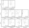 |
Fig. 12 Correlations in the HARPS-N data between the RVs (labeled as RV_srv and the activity indicators listed in Sect. 3.1.2. The Pearson correlation coefficient is indicated in each panel. |
5.3 Limits to secondary eclipses
In the following, we first estimate the maximum secondary eclipse depth of planet b that can be expected, and then revise the TESS light curve for the presence of such eclipses. The depth of a planet’s eclipse behind its host-star is given by the brightness of the planet relative to the star, with the planet’s brightness being the sum of its emitted thermal emission and the amount of stellar light that is reflected from the planet. Regarding thermal emission, Table 8 indicates an equilibrium temperature of 1517 K for planet b, which was calculated for a zero Bond albedo and assuming a uniform heat redistribution over its entire sphere (corresponding to a heat recirculation efficiency of f = 1/4; e.g., Cowan & Agol 2011). For the estimation of the maximum secondary eclipse depth from thermal emission, we assume however a realistic maximum temperature of 1900 K, which is based on the assumption that none of the absorbed radiation gets circulated to the planet’s night-side (corresponding to a value of f = 2/3). Based on that temperature, and using again the adopted parameters from Table 8, we find that thermal emission from planet b may generate eclipses with a depth of only 1.2 ppm in the wavelengths of the TESS bandpass. For a maximum value of secondary eclipse depth from reflected light, a geometric albedo of 1 is assumed, which leads to an eclipse depth of 14 ppm.
Combining thermal and reflected light, we conclude that secondary eclipses of TOI-1416 b may not exceed a depth of 15 ppm. This value might barely be detectable in the light curve. For its detection, we assume that the secondary eclipse is well centered on an orbital phase of 0.5, and generated a phase-folded light curve similar to the one whose preparation is described in Sect. 2 and that is shown in Fig. 1, but now centered at phase 0.5. The fluxes within the expected phase-range of total eclipse (phases from 0.48 to 0.52) were then obtained, which resulted in a flux that is 30±25 ppm higher than the off-eclipse flux. Hence, a secondary eclipse was not detected, and we may estimate that secondary eclipses deeper than ≈20 ppm can be excluded with a high (2-sigma) confidence from the observed data.
Models evaluated with pyaneti.
6 Results and their interpretation
Final system parameters. As the two sets of analysis performed with pyaneti and UTM/UFIT (Appendix C) show in Table 7, no relevant differences arose in those parameters that depend on the TESS light curve; with pyaneti employing GPs and UTM/UFIT a white-noise model on a light curve that had undergone a prior filtering against signals that were significantly longer than the transit-duration. The same goes for the RV fit to TOI-1416 b, where pyaneti and the FCO method – which is essentially a bandpass filter at the planet’s period – obtained very similar results. This outcome is similar to one on TOI-1235 b, where Bluhm et al. (2020) adopted a white-noise-only fit to the TESS light curves, after finding no relevant difference to results obtained from fits based on GPs. For the finally adopted values in Table 8, we quote however those from pyaneti, as only this procedure produced an integral analysis of the combined set of light curves and RVs that was also suitable to evaluate the various models involving a signal from a potential additional planet, c. This planet remains however tentative due to strong doubts that its signal might arise from contamination by the Moon. Furthermore, with the current data we are not able to ascertain if the tentative planet’s period would be 29.5 or 27.4 days.
Such a second planet with a large period ratio of ≈26 against the inner planet would however not be unexpected; the preference for USPs for companions with relatively large period-ratios has been known since the first description of USPs (Sanchis-Ojeda et al. 2014; Winn et al. 2018). From the absence of transits of c, a maximum orbital inclination of 88.7° can be determined. Dai et al. (2018) find that in USPs with a further transiting planet, the systems with the largest period-ratio also tend to have larger mutual inclinations of ≳7°. However, the TOI-1416 system is inconclusive in that respect: With TOI-1416 b’s inclination of 85.7°, even a fully coplanar planet c would not have caused any transits and no conclusions about the system’s mutual inclination, or about limits to it, can be made. The RV fits for an eventual planet c were compatible with eccentricities up to 0.6, which upon the availability of more reliable RV results might lead to the establishment of a formation pathway for TOI-1416 b.
Composition of TOI-1416 b. For the transiting planet TOI-1416 b, its radius of 1.62 ± 0.08 R⊕ and mass of 3.48 ± 0.47 M⊕ indicate that it is a short-period super-Earth-like planet, with a density of  g cm−3. Figure 14 shows a mass-radius (MR) diagram with several composition models from Zeng et al. (2016, 2019). We note that TOI-1416 b is above the line for a purely rocky (100% Mg Si O3) composition, with a density that is about 67% of that of an Earth-like composition (Fig. 15). This separates TOI-1416 b from most other short-period planets: Dai et al. (2019) found for a sample of comparable Hot Earths (11 planets with insolations >650 times that of the Earth and periods of ≲2 days) that most of these are consistent with an Earth Like composition of 30% Fe–70% Mg Si O3. We also use the HARDCORE tool (Suissa et al. 2018), which exploits boundary conditions to bracket a planet’s minimum and maximum core radius fraction (CRF), assuming a fully differentiated planet and iron to be the core material. For TOI-1416 b we obtain a marginal (most likely) CRF of 0 35 ± 0 20. Similar to the planet’s density, this is slightly less than but within the limits of the Earth’s CRF of 0.55, whereas the potential minimum and maximum values of the CRF are zero and 0.71, respectively. Following Zeng & Jacobsen (2017), we may also derive the core mass fraction (CMF) from the approximation CMF ≈CRF2, leading to a value of
  . This value is again relatively small in comparison to the sample of Hot Earths by Dai et al., who determined for them a mean CMF of 26% with a standard deviation of 23%.
We also determined the planet’s restricted Jeans escape parameter, given by  , where Teq is the planets’ equilibrium temperature, mH the mass of the hydrogen atom,G the gravitational constant, and kB the Boltzmann constant (Fossati et al. 2017). The parameter Λ is a global one for a given planet, without dependence on altitude within the atmosphere. Fossati et al. find a critical value of ΛT = 15–35, with smaller values indicating that a planet’s atmosphere is unstable against evaporation, with the planet being in a boil-off regime that shrinks its radius within a few hundred megayears. For TOI-1416 b, Λ = 10.7; it is hence unlikely to have retained a hydrogen-dominated atmosphere that could contribute significantly to its mass or radius. For highly irradiated planets, the evaporation of hydrogen might however lead to an enrichment of other light elements, be it helium, or oxygen from the thermolysis of H2O. For these elements, the hydrogen mass mH in the equation above can be replaced with the element’s atomic mass. For TOI-1416 b, we then obtain values of Λ ≈ 40 and 160 for helium and oxygen, respectively, meaning that these elements are not affected by evaporation.
With TOI-1416 b having at most a small core and a density that is lower than a composition exclusively of silicates requires, but also orbiting too close to the central star to enable the retention of a significant H - He atmosphere, the most likely explanation is the presence of a significant mass-fraction of H2O or other volatiles. Under this assumption, several types of planet compositions have been brought forward: For one, the original and widely discussed models of rocky cores of various fractions of iron and silicates, with mantles of condensed water, (e.g., Seager et al. 2007; Mordasini et al. 2012; Zeng & Sasselov 2013; Zeng et al. 2016). For planets that are more irradiated than the runaway greenhouse irradiation limit of ≈1.1 S⊕, Turbet et al. (2020) provide MR models of silicate cores with mantles of various fractions of H2O in the form of steam, which leads to larger planet sizes for a given mass-fraction of H2O than in the condensed-water models. The work by Turbet et al. provides a procedure to generate MR relations of steam planets for insolations from ≈1 to 30 S⊕. An extension of this work to highly irradiated planets, such as TOI-1416 b with 880 S⊕, is still pending, and the feasibility of a steam atmosphere at the insolation and temperature of TOI-1416 b would have to be shown.
With its equilibrium temperature of 1517±39 K, TOI-1416 b is likely to consist of molten rock (magma) at – or closely below – the surface. We also note that tidal heating might contribute a significant further source of internal heating that is potentially capable of melting a USP’s entire interior (Lanza 2021). Magma has been shown to be able to absorb significant quantities of H2O (Papale 1997; Kite et al. 2020), with the presence of H2O as a likely consequence of in situ water production by a magma-hydrogen reaction, initially proposed by Sasaki (1990, see also Ikoma & Genda 2006; Kite & Schaefer 2021). The presence of such water may lead to radius-increments of up to 16% over interior compositions that do not take dissolved water into account (Dorn & Lichtenberg 2021). In Figs. 14 and 15, we include the MR relation from Dorn & Lichtenberg for their favored “wet-melt” interior (their model C), which assumes the dissolution of water in an Earth-like magma, with various water mass-fractions. This model provides a close agreement with the mass and radius of TOI-1416 b, and hence provides the interpretation of TOI-1416 b’s composition that we favor in this work: A planet of partially solid and molten interior of Earth-like composition, with water being distributed between mantle melt and a surface steam layer, with a total water mass-fraction16 of 1–15%. A more detailed modeling of TOI-1416 b’s composition is beyond the scope of our present work and would also have to take into account the potential range in values of the CMF, and hence the range in the iron/silicate fraction. Potential outcomes could be a relatively small core, with the average density of TOI-1416 b dominated by silicates, or a larger core that requires a larger contribution of H2O to offset the high density of iron.
Suitability for atmospheric characterization. The suitability of a target for its atmospheric characterization by spec-troscopy during a transit has been parametrized by Kempton et al. (2018) with the transmission spectroscopy metric (TSM). The TSM of TOI-1416 b is 83, so it could be a suitable target for such observations with the James Webb Space Telescope (JWST)17. We also note that its emission spectroscopic metric (ESM) is 13.8, which is well above the threshold of 7.5 that Kempton et al. (2018) recommend for the top atmospheric characterization targets for JWST follow-up, albeit for a sample of slightly smaller planets with Rp < 1.5 R⊕. Neither the TSM nor the ESM consider the orbital period, with the TSM relating to the S/N from observing a single transit. Hence, USPs have the further advantage that more transits or orbital revolutions can be acquired in a given time span. In conclusion, TOI-1416 b might be a very suitable target for JWST follow-up.
Position of TOI-1416 b and c relative to the radius valley. Planet b is located slightly below (Fig. 16, top panel) the MR valley (also known as the radius gap or Fulton gap; Fulton et al. 2017; Van Eylen et al. 2018; Petigura et al. 2022) near radii of 2 R⊕ that separates the population of super-Earth planets from the larger sub-Neptune-like planets. At the short orbital period of TOI-1416 b, the valley is however poorly defined and only a population of smaller planets remains (see also Fig. 17). On the other hand, for the tentative planet c, with its mass of M sin i ≈ 22 M⊕, we estimate a radius of 5.5 ± 2.5R⊕ from the radius-mass relation by Chen & Kipping (2017). This indicates a Neptune-like planet that would lie well above the MR valley and would convert TOI-1416 into a system with a near-USP below the radius valley and a second planet that is above it. Of course, we do not know the size of the tentative planet c, but a radius that would place it below the radius valley would have to be smaller than ≈1.7 R⊕. Such a small radius is unrealistic from both the observed radius-mass relation and from the required densities in excess of 20 g cm−3; hence this outcome can be excluded with near-certainty.
The Neptune Desert and its borders. In the planet radius and planet mass versus period diagrams (Fig. 16), we note the well-known “Neptune Desert” as defined by Mazeh et al. (2016), with the lower boundary for the planet radius given by log Rlo/R⊕ = 0.68 log P, with P given in days, and the lower boundary in the mass-period planet given by log Mlo/Mjup = 0.98* (log P) − 1.85. However, given the mass and period distributions in Fig. 16, which contain many recently discovered planets with periods ≲1 day, we doubt the validity of the lower boundaries for periods shorter than ≈2 days, because most of the known USPs, including TOI-1416 b, would be within the “desert.” Indeed, only a few years ago the period regime below 1 to 2 days was only sparsely populated by small planets of <1.6 R⊕. This also gave rise to statistical evaluations claiming that P≈ 1 day separates the shortest period planets regarding their size and numbers against the slightly longer-periodic planets (Pu & Lai 2019; Winn et al. 2018; Lee & Chiang 2017). One of the principal impacts of the TESS mission has, however, been the discovery of over 20 planets with P ≲ 1 days since the year 2020 that, furthermore, have mass measurements from ground-based follow-up. In the period regime of P ≤ 2 days, we hence propose replacing the desert’s lower boundary with a constant that corresponds to the desert’s lower boundary at P = 2 days for both radius and mass, leading for P < 2 days to a boundary at a radius of 1.60 R⊕ (log Rlo/R⊕ = 0.2) and a mass of 0.028 Mjup (log Mlo/Mjup = −1.55), or 8.9 M⊕ (dotted lines in Fig. 16). In support of these lower limits to the desert, Fig. 17 (top panel) shows the radius distribution of the short-period small planet population with log R/R⊕ < 0.8, where we note that the radius distribution has only a weak dependence on the orbital period, with the planet’s median size following the relation

We show in Fig. E.1 a plot similar to that of Fig. 16, but against the planets’ insolation and effective temperature, where the upper boundary of the Neptune Desert has become notably better defined, and propose corresponding limits of the Neptune Desert against these parameters.
From these distributions, it appears that TOI-1416 b belongs to a continuous distribution of super-Earths with periods ranging from the shortest known ones up to ≈30 days, with neither the period-radius nor the period-mass distributions showing any signs of a discontinuity near the common limit of P = 1 days for USPs. The maximum radii of super-Earths are delimitated at the shortest periods by the Neptune Desert (for which we propose a lower limit of ≈1.6 R⊕ for P < 2 days, although planets with radii of up to ≈2 R⊕ would belong to the same population18), while for longer periods, super-Earth radii are delimited by the period-radius valley that separates them against sub-Neptune type planets.
Distribution of small planets against period and USP formation pathways. Regarding the abundance of small planets against period (Fig. 17, bottom panel), we note the emergence of a plateau between log P of −0.125 and +0.125 (P ≈ 0.6−1.4 days). This plateau might correspond to a previously noted “bump” of about 50% in planet counts just below P = 1 day, relative to slightly longer periods (Pu & Lai 2019; based on the work by Lee & Chiang 2017)19, with abundance slopes that are steeper below 1 day than above 1 day. The newer planet discoveries imply however that this bump has smoothed out into the observed plateau, whereas the abundance slope remains somewhat steeper to the left than to the right of the plateau. Alternatively, there might be a uniform slope in abundances against period, with an additional accumulation of planets at periods between 0.6 and 1 day.
Pu & Lai (2019) proposed the formation of USPs within multi-planet systems from low-eccentricity migration due to secular interactions among the planets. This pathway involves an innermost planet that is born with a period of several days and a moderate eccentricity of 0.05 to 0.15. Through tidal interactions with further outer planets, the eccentricity of the innermost one is gradually damped to nearly zero, while its semimajor axis undergoes a quasi-equilibrium shrinkage. As a result of this process, the innermost planet transforms into a USP, while the outer planet stabilizes at an orbital period that is larger by ≳15 times. Pu & Lai (2019) also provide synthetic planet distributions that have undergone this formation pathway, with a variety of initial parameters (varying the mass and eccentricity of the innermost planets and also the tidal quality factor, Q, of both stars and inner planets). It is of note that their simulation with the highest initial orbital eccentricity, of 0.15±0.025 (their Fig. 15), agrees very well with the observed abundances from Fig. 17, reproducing the abundance plateau around P ≈ 1 day and the steeper slope to the left than to the right of it. Notably, the initial eccentricity was identified by Pu & Lai (2019) as the parameter that most clearly affected the final results of their simulations. This leads to the suggestion that USP formation from inward migration of inner planets with an initial eccentricity of ≈0.15 might be a common one. Several further formation pathways have been proposed in the literature, with a notable contrast being the high-eccentricity pathway by Petrovich et al. (2019) that requires an initial eccentricity of e ≳ 0.8. However, without simulated planet distributions against basic parameters such as period, radius, and mass being available, the presence of these pathways needs to be evaluated from other diagnostics, such as ratios of orbital periods or mutual inclinations between inner and outer planets, or measurements of spin-orbit angles, which are beyond the scope of the present work.
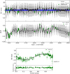 |
Fig. 13 Modeling of HARPS-N spectroscopy with pyaneti. Upper panel: RV and dLW time series for Model 1, assuming only the presence of a Keplerian signal with the 1.07 days transit period. The green markers in each panel represent the RV and dLW measurements. The solid black curve shows the inferred multi-GP model, with dark and light shaded areas showing the one and two sigma credible intervals of the corresponding GP model. We note that the short period of the planet and the size of the plot make the RV sinusoids appear as a solid blue band. Lower panel: HARPS-N RV data folded on the 1.07-day orbital period of planet b, after subtraction of the systemic velocity and the GP noise model. The inferred RV model is shown as a solid black curve with 1- and 2-sigma credible intervals (shaded areas). |
Priors and inferred parameters from transit and RV modeling with pyaneti (Model 3) and UTM/UFIT or FCO.
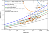 |
Fig. 14 Planet masses and radii, versus composition models: Gray markers indicate planets with well-determined masses (errors smaller than 30%, from adopted values in the NASA Exoplanet Archive). Planets with periods of less than 2 days are shown with brown markers. Composition models indicated by solid lines are from Zeng et al. (2016, 2019), whereas the dashed line is a model from Dorn & Lichtenberg (2021) for an Earth-like rocky composition (66% Mg-Si oxides and silicates and 33% iron), where the molten rock contains water with a mass fraction of 5.4%. TOI-1416 b is indicated by the red dot. |
Adopted derived parameters.
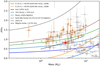 |
Fig. 15 Like Fig. 14, but in mass-density space, with the density given relative to the Earth’s density of 5.51 g cm−3. |
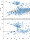 |
Fig. 16 Diagram of the radii (top panel) and. masses (bottom panel) versus period of the known planets, from the NASA Exoplanet Archive. The solid black lines show the delineation of the “Neptune Desert” from Mazeh et al. (2016), whereas the horizontal dotted black lines show the lower limits to the Neptune Desert for periods ≤2 days that are proposed in this work. The dashed orange line in the upper panel indicates the period-radius valley from Van Eylen et al. (2018). TOI-1416 b is indicated by the filled red circle and the tentative planet c by the unfilled one. |
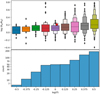 |
Fig. 17 Distributions of small planets of log R/R⊕ < 0.8 (or R/R⊕ < 6.3) and with periods shorter than 3.6 days, after categorizing their population into bins with a width of log P(day) = 0.125. Top panel: Distribution of planet radii against the orbital period. The distributions are shown as “boxenplots” or “letter value plots” (Hofmann et al. 2011). TOI-1416 b is indicated by the red star. Bottom panel: Counts of the small planets versus the same bins in orbital period. |
7 Conclusions
We report the discovery of the super-Earth planet TOI-1416 b, which is orbiting with a period of 1.07 days around a middle-aged G9V star that likely belongs to the galactic thin disk, and a tentative second planet, c, of Neptune-like mass and a period of 27.4 or 29.5 days. The highest peaks in the RV periodograms and Keplerian fits for c indicate a best-fit period that coincides very closely with the lunar synodic period. Consequently, the true nature of c remains tentative despite an intense campaign of RV observations, because contamination of the RV data by a signal arising from Moon-reflected solar light cannot be ruled out. If planet c is real, its radius of 3–8 R⊕ would position it above the period-radius valley, while planet b is below the valley, albeit in a zone in the period-radius plane where the valley is only poorly defined.
Several composition models are discussed for TOI-1416 b. Given the expected high temperature of both the planet surface and interior, we consider a model that describes a molten interior in which a significant fraction of water is dissolved in magma as the most promising to explain the planet’s density, which is significantly below the density expected for a pure silicate composition. If the planet has an atmosphere, it is unlikely to contribute significantly to the planet’s mass but it could be suitable to observation by transmission spectroscopy with the JWST, and the planet’s surface might be within the reach of emission spectroscopy.
The lower limit of the Neptune Desert, initially identified by Mazeh et al. (2016), was revised for planets with periods of less than 2 days. For them, the original definition of the lower boundary is clearly inconsistent with recent discoveries of significant numbers of short-period planets. For periods of P < 2 days, a lower boundary to the desert at a radius of 1.60 R⊕ and a mass of 8.9 M⊕ is therefore proposed. We also delimit the desert using the planets’ insolation instead of the period as a basic parameter. In both radius versus insolation and mass versus insolation distributions, the upper limit of the desert is more pronounced, and we give the corresponding relations that delimit the desert against insolation and against the planets’ effective temperatures.
The borderline position of TOI-1416 b just outside the conventional definition of USPs as planets with P ≤ 1 day motivated an evaluation of its position within the planet population, in both period-radius and period-mass diagrams. From these, we deduce that planets with periods of less than one day do not constitute a special group of planets. Rather, USPs appear to be the extreme end of a continuous distribution of super-Earths, with periods extending from the shortest known ones up to around 30 days, with upper radii limited by the Neptune Desert for periods shorter than ≈2 days, and by the period-radius valley for longer periods. Within the super-Earths, subgroups with specific properties may, however, become increasingly better characterized, depending on the insolation, type or age of the central star, and/or the presence of additional planets. One such hint is the plateau that has emerged in the relation between small-planet abundance and period, in a range from 0.6 to 1.4 days, and which is compatible with the low-eccentricity formation pathway proposed by Pu & Lai (2019). The recent discoveries of numerous short-period planets, such as TOI-1416 b, should inspire comprehensive investigations into the suitability of the various proposed formation mechanisms in explaining the present distribution of these planets across the broadest spectrum of parameters feasible.
Acknowledgements
This work was supported by the KESPRINT collaboration, an international consortium devoted to the characterization and research of exoplanets discovered with space-based missions (http://www.kesprint.science). This paper includes data collected by the TESS mission. Funding for the TESS mission is provided by the NASA Explorer Program. We acknowledge the use of public TOI Release data from pipelines at the TESS Science Office and at the TESS Science Processing Operations Center. Resources supporting this work were provided by the NASA High-End Computing (HEC) Program through the NASA Advanced Supercomputing (NAS) Division at Ames Research Center for the production of the SPOC data products. This research has made use of the Exoplanet Follow-up Observation Program (Exo-FOP; DOI: 10.26134/ExoFOP5) website, which is operated by the California Institute of Technology, under contract with the National Aeronautics and Space Administration under the Exoplanet Exploration Program. This work has made use of data from the European Space Agency (ESA) mission Gaia (https://www.cosmos.esa.int/Gaia), processed by the Gaia Data Processing and Analysis Consortium (DPAC, https://www.cosmos.esa.int/web/Gaia/dpac/consortium). Funding for the DPAC has been provided by national institutions, in particular the institutions participating in the Gaia Multilateral Agreement. Based on observations made with the Italian Telescopio Nazionale Galileo (TNG) operated on the island of La Palma by the Fundación Galileo Galilei of the INAF (Instituto Nazionale di Astrofisica) at the Spanish Observatorio del Roque de los Muchachos of the Instituto de Astrofísica de Canarias under programmes CAT19A_162, CAT21A_119, CAT22A_111 and ITP19_1. CARMENES is an instrument for the Centro Astronómico Hispano-Alemán de Calar Alto (CAHA, Almería, Spain). CARMENES is funded by the German Max-Planck-Gesellschaft (MPG), the Spanish Consejo Superior de Investigaciones Científicas (CSIC), the European Union through FEDER/ERF FICTS-2011-02 funds, and the members of the CARMENES Consortium (Max-Planck-Institut für Astronomie, Instituto de Astrofísica de Andalucía, Landessternwarte Königstuhl, Institut de Ciències de l’Espai, Institut für Astrophysik Göttingen, Universidad Complutense de Madrid, Thüringer Landessternwarte Tautenburg, Instituto de Astrofísica de Canarias, Hamburger Sternwarte, Centro de Astrobiología and Centro Astronómico Hispano-Alemán), with additional contributions by the Spanish Ministry of Economy, the German Science Foundation through the Major Research Instrumentation Programme and DFG Research Unit FOR2544 “Blue Planets around Red Stars”, the Klaus Tschira Stiftung, the states of Baden-Württemberg and Niedersachsen, and by the Junta de Andalucía. This article is partly based on observations made with the MuSCAT2 instrument, developed by ABC, at the Telescopio Carlos Sánchez operated on the island of Tenerife by the IAC in the Spanish Observatorio del Teide. This work makes use of observations from the LCOGT network. Part of the LCOGT telescope time was granted by NOIRLab through the Mid-Scale Innovations Program (MSIP). MSIP is funded by NSF. We thank the following iSHELL observers: Kevin I Collins, Michael Reefe, Farzaneh Zohrabi, Eric Gaidos, Angelle Tanner and Claire Geneser. We thank Annelies Mortier for the provision of the latest versions of her code for the BGLS and related plots. H.J.D. and S.M. acknowledge support from the Spanish Research Agency of the Ministry of Science and Innovation (AEI-MICINN) under grant ‘Contribution of the IAC to the PLATO Space Mission’ with references ESP2017-87676-C5-4-R and PID2019-107061GB-C66, DOI: 10.13039/501100011033. S.M. and D.G.R. acknowledge support form the same source with the grant no. PID2019-107187GB-I00. S.M. acknowledges support from the same source through the Severo Ochoa Centres of Excellence Programme 2020–2023 (CEX2019-000920-S). P.G.B. acknowledges support from the same source with the Ramóny Cajal fellowship number RYC-2021-033137-I. G.N. thanks for the research funding from the Polish Ministry of Education and Science programme the “Excellence Initiative – Research University’ conducted at the Centre of Excellence in Astrophysics and Astrochemistry of the Nicolaus Copernicus University in Toruń, Poland. This work is partly supported by JSPS KAKENHI Grant Number P17H04574, JP18H05439 and JP20K14521, and JST CREST Grant Number JPMJCR1761. J.M.A.M. is supported by the National Science Foundation Graduate Research Fellowship Program under Grant No. DGE-1842400. J.M.A.M. acknowledges the LSSTC Data Science Fellowship Program, which is funded by LSSTC, NSF Cybertraining Grant No. 1829740, the Brinson Foundation, and the Moore Foundation; his participation in the program has benefited this work. K.A.C. and D.W.L. acknowledge support from the TESS mission via sub-award s3449 from MIT. K.W.F.L. was supported by Deutsche Forschungsgemeinschaft grant RA714/14-1, within the DFG Schwerpunkt SPP 1992, “Exploring the Diversity of Extrasolar Planets’. J. K. gratefully acknowledges support by the Swedish National Space Agency (SNSA; DNR 2020-00104) and by the Swedish Research Council (VR: Etableringsbidrag 2017-04945).
Appendix A Stellar rotation period
We determine the rotation period from the light curve of TOI-1416 by following the procedure described in Santos et al. (2019) and Santos et al. (2021, see also Mathur et al. 2014 and García et al. 2014a). The analysis was based on TESS light curves that have undergone after the same processing as described in Sect. 2 for the analysis with pyaneti, from which we removed the exo-planet transits to avoid spurious signals (using the best-fit model obtained with UTM/UFIT as described in Appendix C). Due to the small number of data points that remained in Sector 50 after removal of the bad quality data, only Sectors 16 and 23 were used for the rotational analysis. Also, gaps in the light curve longer than 81 days (three consecutive TESS sectors) were removed, and inpainting techniques were used to fill in gaps shorter than 5 days (García et al. 2014b), leading to the light curve shown in the top-panel of Fig. A.1. From this curve, we derive three estimates of the rotation period: The first estimate is obtained from the global wavelet power spectrum (GWPS; Torrence & Compo 1998; Mathur et al. 2010), which examines the correlation between the data and the mother wavelet (taken to be a Morlet wavelet), and its projection onto the period axis. The second estimate is obtained via the autocorrelation function (ACF; McQuillan et al. 2013, 2014), which computes the correlation between the light curve and itself for a range of time shifts. The third estimate is obtained from the composite spectrum (Ceil-lier et al. 2016), which is calculated as the product between the GWPS and the normalized ACF and helps to enhance the periods that are present in both methods.
Figure A.1 shows the results from all three methods. From the ACF analysis, we can see three peaks with prominent absolute amplitudes. However, as shown in Ceillier et al. (2017), one of the criteria to select reliable rotation periods is based on the relative amplitudes of the peaks, called H_ACF, with significant periods having values of H_ACF > 0.3. Computing the H_ACF for these three peaks, the largest value is found for the period corresponding to 17.6 ± 2 days (with a value of H_ACF = 0.5). That is the period we adopt, which approximately corresponds to the third harmonic of the ≈5 day signal seen in both the ACF and the global wavelet power spectrum (GWPS). Moreover, García et al. (2021) applied the same method to over 2 million “Kepler-seen-as-TESS” light curves, for stars for which rotation periods had been measured by Santos et al. (2019, 2021). They divided the full Kepler light curves into 27-day chunks to mimic the TESS observations, and their results showed that periods of up to ≈20 days can be retrieved with one sector of data. For instance, for peaks with H_ACF > 0.3, they recovered periods in the 10 to 15 day window with a reliability of ≈70%.
We note that our adopted 17.6 ± 2 days ACF period is also compatible with the rotation period of  d determined from V sin i⋆ and R⋆ of Tables 4 and 5. While the 17.6 day period does not show up in the GWPS, this is unsurprising as it would have been filtered out due to falling outside the cone of validity (hatched regions in Fig. A.1; see also García et al. 2021). Regarding a ≈ 10 day stellar rotation that would correspond to the second harmonic of the ≈5 day signal and for which activity indicators from the RV data indicate a notable peak in spectrograms (Sect. 5.1), it is argued at the end of Sect. 5.2 that this period is unlikely to be associated with stellar rotation.
From the adopted period of 17.6 d, we furthermore derived ages from several rotation-age relations reported in the literature, resulting in ages of: 0.84 ± 0.18 Gyr (Barnes 2007); 1.26 ± 0.29 Gyr (Mamajek & Hillenbrand 2008); 1.58 ± 0.7 Gyr (Angus et al. 2015); 1.49 ± 0.23 Gyr (Angus et al. 2019); and 1.75 ± 0.25 Gyr (Spada & Lanzafame 2020). Ignoring the value from Barnes (2007) as the most discrepant one, gyrochronology indicates hence an age of 1 – 2 Gyr. We note however that the light curve analysis does not exclude a longer rotation period that is not perceived due to the limited coverage of the TESS light curves and which would also indicate older ages for TOI-1416.
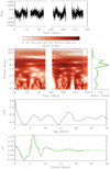 |
Fig. A.1 Analysis of TESS light curve for stellar rotation of TOI-1416. The top panel shows the light curve from Sector 16 and 23 that was used for the analysis. The following panels show the three methods used for the period determination (see the main text): the GWPS and its projection onto the period axis; the ACF; and the composite spectrum (CS). The hatched region in the panel for the GWPS indicates the zone where the method is not valid. |
Appendix B The RV double peak at periods of 27.4 and 29.5 days: Planet candidate or influence from the Moon?
The spectral signatures presented in Sect. 5.1, from both the BGLS and the Bayes factor periodogram from agatha indicate an RV signal in the HARPS-N data with a period of ≈29.5 d as the most promising one for an additional planet in TOI-1416. Figure B.1 shows a zoom of the BGLS periodogram near that period, which also shows the somewhat lower neighboring RV peak with P= 27.4 days. Potentially, one of these peaks (more likely the lower 27.4 d one) is an alias of the other one, related to each other by a seasonal sampling with a frequency of 1/365 d−1.
Of principal concern regarding the interpretation of the 29.5 d peak is its close match with the length of the lunar synodic month of 29.53 d, which in the case of the 29.52 d signal found by agatha (see Fig. 11) is matched to the fourth digit. We also note a relative strong peak of the CRX activity indicator near that period. Considering also TOI-1416’s small systemic RV of ≈1.1 km s−1, this leads to a strong suspicion that the observed RV peak might be due to a contamination by the Moon, or more precisely, be due to the influence of solar light that is reflected by the Moon. In Fig. B.2 we show a plot of the uncorrected observed RVs of TOI-1416 against the (calculated) RV of the Moon-reflected solar spectrum at the moment of observation. For differences between these two RVs of ⪅ 10 – 15 km/s, spectral lines in the reflected solar spectrum might overlap with similar lines in the target’s spectrum20 and hence might affect the measured RVs. We note in Fig. B.2 that the “above horizon” RVs of the target and of the Moon-reflected solar spectrum are correlated21. This effect is due to a relation between the observational season and the preferential lunar phase: At the begin of the target’s seasonal visibility, observations are taken in the morning, when only a waning moon might be above the horizon, and the solar spectrum reflected by a waning Moon always has a negative RV (because the path Sun-Moon-Earth gets shorter). At the begin of seasonal visibility, Earth moves also toward TOI-1416, resulting in a negative observed RV. During the middle of the observational season, the target might be observed at any lunar phase, and toward the end of the season, the target is only visible at the begin of the night when only a waxing moon might be above horizon, and the corresponding RVs are reversed.
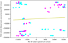 |
Fig. B.2 Observed uncorrected RVs of TOI-1416 versus calculated RVs of the Moon-reflected solar spectrum. The symbol colors indicate if the Moon was above (pink) or below the horizon (blue) at the moment of observation. The green line corresponds to identical RV values on both axes. |
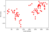 |
Fig. B.3 HARPS-N RVs folded against the lunar phase, where 0° or 360° corresponds to New Moon and 180° to Full Moon. The clumping of the RV data in two regions of lunar phases, with an avoidance of Full Moon and lesser coverage near New Moon, is a consequence of the scheduling of the HARPS-N observations, which were mostly executed in lunar gray time. |
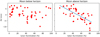 |
Fig. B.4 Similar to Fig. B.3, but the HARPS-N RVs are plotted against the lunar illumination at the time of observation, and the data are separated into panels containing only RVs that were taken when the Moon was below or above the horizon. The blue line in the right panel shows a linear fit to the RV versus illumination dependence, which has a correlation coefficient of −0.69. |
Using the hypothesis of a contamination by the Moon, the barycentric-corrected HARPS-N RV values22 were folded against the lunar synodic period, with their time-stamps converted to corresponding values of lunar phases. The result (Fig. B.3) shows a clear dependence between lunar phase and RV, with a symmetry against the full or the new Moon. However, this does not disprove that by coincidence, a planet in TOI-1416 might have a period that is very close to the lunar one. In a further step (Fig B.4), we separated the RVs into those that were taken with the Moon being above horizon (46 RV points) and those where the Moon was below horizon (50 points). Also, instead of the lunar phase, we plot the RVs against an approximation of the lunar illumination, given by the relation
 (B.1)
(B.1)
where φ is the lunar phase in radians, with φ = 0 at New Moon. The result shows no relevant correlation (with a correlation coefficient of −0.23) for the RVs against illumination (or phase) when the Moon was below the horizon23. However, a relevant correlation (with a coefficient of −0.69) is present when the Moon was above the horizon. Corresponding BGLS spectra for the RVs with/without Moon (Fig. B.5) show the 29.5 d peak very prominently in the “above horizon” spectrum, whereas in the “below horizon” spectrum, the 29.5 day peak is insignificant while the peak at 27.4 d has become more prominent and a second one at 32.2 d has appeared. The 32.2 d peak might be another alias of the 29.5 d peak against a yearly sampling frequency, but we also note the strongly disparate window-function between the 27.4 and the 32.2d peaks, which weakens any conclusions regarding the relations between these peaks. In any case, the prominence of the 29.5 d signal in the above horizon spectrum and its disappearance in the below horizon one, together with the correct phasing of this signal against the Moon’s illumination is a strong indicator that the Moon is indeed responsible for this signal.
Dependences of the RVs against the Moon altitude at the time of observations or against the angular separation of the Moon and TOI-1416 were evaluated as well, but these do not show any relevant correlation. Attempts were made to correct the above-horizon RVs against the illumination-dependence, using the linear fit shown in Fig. B.4 (and also trying higher-order fits, not shown) and to perform a modeling with pyaneti on the corrected RVs. The results were however unsatisfactory, showing only degraded fits for a Keplerian signal at either the 29.5 or 27.4 d period.
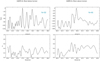 |
Fig. B.5 BGLS periodograms of the HARPS-N RVs and window functions, with the RV data separated into those taken when the Moon was below and above the horizon. The blue numbers indicate the number of RV points. |
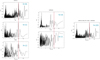 |
Fig. B.6 BGLS periodograms of the RVs of the contributing instruments. In the left column are those that show a peak near 27 or 29 days (vertical red lines); in the center are those that do not. The right panel shows a periodogram with the RVs from all instruments combined. The blue numbers indicate the number of RVs used. |
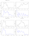 |
Fig. B.7 Development of the S/N (black curves) and the best-fitting amplitude “bestK” (blue curves, in m/s) of RV signals with periods of 27.40 d (top set of panels) and 29.53 d (bottom set), versus the number of RV points since the first measurement. The left panels are based on RVs from HARPS-N and the right ones on RVs from the APF. |
In order to identify potential RV shifts due to contamination by the Moon, we evaluated the effect of the Moon on the HARPS-N high-resolution spectra’s CCF. Only in 65 of the 96 HARPS spectra, a second fiber (B) was placed on the sky, and only in a minority of the 65 fiber-B spectra, a signal from the Moon-reflected spectrum could be identified and the RVs be corrected against it. The difference from that correction was almost always below 1 m/s, which is small against the ≈5 m/s amplitude of the 29.5 d signal. Consequently, periodograms with or without this correction in these 65 HARPS-N RV do not show relevant differences. We also investigated if there might a relation between the RVs and the S/N in the spectra (e.g., due to sky-brightness from the Moon) but there is no correlation apparent (for the RVs taken with the most frequent exposure time of 1200 sec, a correlation coefficient of −0.05 was found). Hence, an identifiable effect of the Moon-reflected solar spectrum onto the measured RVs is very minor.
However, we consider that the 29.5 d peak in the HARPS-N spectrograms remains of questionable nature, and now turn our attention to the neighboring peak at ≈27.4 days. Figure B.6 shows BGLS spectrograms of all contributing instruments, and it is of note that data from the APF – which contributed with the second largest set of RVs – have their strongest peak at 26.8 d. Also, the HIRES RVs show a peak in the same period-range, which is very broad due to the small sample of only 12 RVs. However, peaks in that range are absent in periodograms from CARMENES and iSHELL data. We note that these are also the instruments whose spectral coverage is the most red-ward (see Table 3), and a Moon-reflected reflected solar spectrum would generate a weaker signal in them. Lastly, in a combination of all available RVs, the peak at 27.4 d is the highest overall, and is significantly stronger than the one at 29.5 d.
In Fig. B.7 we provide plots of the development of the S/N and the best-fitting amplitude K of the RV signal at periods of 27.40 and 29.53 days, versus the number of RV points (counting from the first measurement), following the precepts of Mortier & Collier Cameron (2017). These plots are shown for the two largest sets of RVs, those from HARPS-N and from the APF. In the plots for HARPS-N, the S/N degrades at either period near the 40th point, which is likely due to a lesser consistency of these signals across RV coverages spanning more than one observing season. On the other hand, in the plots for the APF (which cover only one observing season), the 27.4 d signal shows a steady increase in S/N and a rather constant amplitude K, whereas the 29.5 d signal shows a less consistent picture, more similar to the one from HARPS-N. As is stated in Sect. 5.2, fits of Keplerian orbits to the 27.4 d signal where however significantly worse than those to the 29.5 d one.
In summary, we cannot decide on a clear preference that either of these signals represent a true signal from TOI-1416, nor about their actual nature, and conclude that the RV signals with a 27.4 or 29.5 day period are at most tentative of an additional planet at either of these periods.
Appendix C Modeling of the light curve with UTM/UFIT
The normalized and gradient-corrected light curve around transits of planet b, whose preparation is described in Sect. 2, was used for transit fits using the Universal Transit Modeller / Universal Fitter (UTM/UFIT; Deeg 2014)24. In brief, UTM is a light curve modeller for all kinds of eclipsing or transiting configurations between any number and kind of objects, such as stars, planets, moons, and rings, written in IDL. UFIT was developed as a wrapper to UTM to perform fits, though it has been extended to accept several further modeling modules (such as the one used for the FCO fit described in Appendix D). As its core modeling engines, UTM can use either pixelized object representations suitable for arbitrary configurations of multiple occulters or an analytical “fast mode” suitable for basic transit configurations, which employs the exofast_occultquad.pro routine from the EXOFAST library (Eastman et al. 2013, 2019); the latter approach was used in this work. UFIT permits the fitting of any of UTM’s input parameters, either with the Amoeba algorithm or through the generation of MCMC chains using the Differential Evolution Markov Chain method of Ter Braak (2006). Its implementation is based on the EXOFAST_DEMC routine from the same library, but with an extension that permits the constraining of free parameters by several types of symmetric and asymmetric priors.
UTM gives complete freedom to the set of parameters that is chosen to model an orbiting system; that is, any set of parameters that is fully able to describe an orbiting system can be used25. For this work, we modeled the TESS light curves against the following set of parameters (these were also free parameters in the fits): orbital period, Porb, transit epoch, T0, scaled planetary radius, Rp/R⋆, the stellar density,26 ρ⋆, and the transit impact parameter, b. Initial values for these fits were taken from the SPOC data validation summary for TOI-1416. For the stellar LD, a quadratic LD law was used, although for the fitting we used the q1 and q2 coefficients for an optimized sampling introduced by Kipping (2013). An absolute offset in flux values was a further free parameter in our fits, in order to account for potential errors in the normalization of the flux described in Sect. 2. The orbital eccentricity was kept to zero.
Initial fits were performed with the Amoeba algorithm, leading to an intermediate transit-model that was used for the initial parameters of an MCMC sequence. First efforts without constraints on the input parameters showed significant correlation between the impact parameter, the stellar density, and the planet radius. Also, the LD parameters could only be poorly constrained from the fits. We therefore chose to impose Gaussian priors on the stellar density (taken from the adopted value in Table 5) and on the LD. For the later, we used the tabulation of LD coefficients for the TESS satellite bandpass by Claret (2017, Table 25 for the ATLAS model with plane-parallel geometry) and an interpolation to the adopted stellar parameters from Tables 4 and 5. The obtained values for a square LD law as defined in Eq. (2) of Claret (2017) were u1 = 0.4545 ± 0.05 and u2 = 0.1880 ± 0.05, which were converted into priors for the q1 and q2 coefficients, given in Table 7.
The final MCMC sequence consisted of 16 parallel chains that were iterated until a sufficient mixing of parameters was achieved, based on the Gelman-Rubin statistics following the precepts of Ford (2006) and Eastman et al. (2013). The resultant values (included in Table 7) were then derived from the posterior distributions of the parameters, based on 4280 steps, after a burn-in period of ≈1000 steps. These distributions were in all cases close to Gaussian shapes (see Fig. C.1 for this and several further diagnostic plots from the MCMC sequence). The best-fit transit model against the phase-folded input light curve is also shown in Fig. 1.
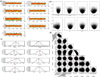 |
Fig. C.1 Graphical output from MCMC sequence performed by UFIT that led to the results reported in Table 7. In all panels, the parameters are indicated by the keywords used in UFIT: “1period” for the planet period, “1trepoch” for the epoch of transit, “1radi” for the relative planet radius, “0densCGS” for the stellar density in CGS units, “1impact” for the impact parameter, “0limbd” and “0limbd2” for the LD coefficients q1 and q2, and “ooff” for the off-transit flux-offset against zero. The sub-figures are: (a) Values of the parameters against link-number of the MCMC sequence, excluding burn-in. Each MCMC chain is shown by a different color. The lowest panel shows the evaluation of the χ2 values. (b) Scatter plot of parameters versus the χ2 value. (c) Histograms of parameter distributions. The median value is shown by the vertical black line; the dashed lines delimit the 68.3% credible interval and the red line gives the value of the best fit. (d) Corner plot of the correlations among parameters. The red crosses give the values of the best fit. |
Appendix D Detection of the transiting planet in RV data via FCO analysis
The FCO (Floating Chunk Offset) method, developed by Hatzes et al. (2010) and Hatzes (2014), is best suited for the determination of RV amplitudes of short-period planets whose nightly RV variations are expected to be larger than the individual RV measures’ uncertainties. In short, sets of nightly RV data – with at least two well-separated data points per night – are treated as independent chunks of data with unknown (free) RV offsets. Systematics (both instrumental and effects from other planets or stellar activity) on timescales larger than a single night are therefore suppressed by the FCO method. RV offsets for each nightly set of RVs are then fitted against an RV model and the parameters of the best fit are obtained.
Only the RVs from HARPS-N were used in this analysis. The FCO method could not be applied to data from the other telescopes, because all their RVs are single data points in a given night (with the exception of two nights from APF, where RVs spaced about 20 min apart were obtained, which is too short a separation to be suitable for the FCO analysis). In the HARPS-N data, there are 28 nights in which two or more RVs were obtained, which enabled the use of 77 out of the 93 RVs from HARPS-N. For the fitting of the RVs, we used the same UFIT-fitter as described in Appendix C, but with the modeler module ufit_rvcurve for the generation of Keplerian RV models from multiple RV data-sets, each with its own RV-offset γi. For the FCO method, each “chunk” with a nightly set of two or more RVs is considered an independent set of data.
A fit using the FCO method for a candidate with an ephemeris known from transits, and assuming a circular orbit is in principle very simple, as it contains as free parameters only the RV amplitude K and the nightly RV offsets γi, with i = 1,…,28 indexing the individual nights. However, when using UFIT with both the AMOEBA or the MCMC fitter, resultant RV amplitudes tended to be stuck close to the amplitude’s initial value. This behavior was caused by the large number of 28 nights, where each one corresponds to a free parameter γi. Due to this, both fitters found it difficult to vary the RV amplitude, since any improvement in the fit requires that most of the nightly RV offsets are changed simultaneously by the correct amounts. This is difficult to achieve for any fitting algorithm, and is an expected behavior when free parameters are strongly correlated. We therefore kept the RV amplitude – and hence the entire RV model -fixed and fitted only for the RV offsets γi, which reduces the fitting task to a set of 28 simple linear fits. The input RV amplitude was then stepped through a series of suitable values and the χ2 of each corresponding fit was logged, which led to the curve shown in Fig D.1. The minimum of this curve, and the range where χ2 increases by 1, indicate an amplitude of Kb = 2.14 ± 0.35 m s−1. For the best-fit model with Kb = 2.14 m s−1, the reduced χ2 is 0.87 and the residuals of the RVs against the model have an rms of 0.82 m s−1. Figure D.2 shows the RVs of the nightly chunks against the best RV model, with a zoomed-out section across three nights of the RV time-series showing the excellent fit in that range. We note that a further FCO fit of the HARPS-N RVs with pyaneti (see Sect. 5.2) gave a nearly identical result, of 2.12 +0.36 m s−1.
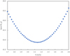 |
Fig. D.1 Best-fit χ2 from FCO fits of HARPS-N data to a series of RV models of TOI-1416 b with fixed RV-amplitudes K. |
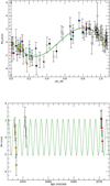 |
Fig. D.2 FCO fit to the HARPS-N RVs. Upper panel: Phase-folded RV model (green line) of TOI-1416 b, which corresponds to the best fit from the FCO method, obtained by vertically offsetting nightly chunks of RV data against the model. RV points from the same nights have identical colors. Lower panel: Small section of the RV model plotted against time, with RVs from three different nights. |
Appendix E The Neptune Desert in radius or mass versus insolation or effective temperature
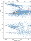 |
Fig. E.1 Similar to Fig. 16, but with planet radii (top panel) and masses (bottom panel) plotted against the planets’ insolation (lower X-axis) and their effective temperature (upper X-axis). The solid black lines show the delineation of the Neptune Desert against insolation and Teff, whereas the horizontal dotted black lines show the same lower limits to the Neptune Desert as those proposed for periods of P ≲ 2d. The dashed orange line in the upper panel indicates the radius valley against insolation from Petigura et al. (2022). TOI-1416 b is indicated by the filled red circle and c by the unfilled one. |
In Fig. E.1 we show plots similar to Fig. 16, but plotting the planets’ radii and masses against the incident bolometric flux or insolation, instead of orbital period. The insolation was calculated from first principles using values obtained from the NASA Exoplanet Archive. It is of note that the upper boundary of the Neptune Desert is significantly sharper than in Fig. 16, whereas the lower boundary remains diffuse; in particular for the plot of planet masses. Given the sharper upper boundary, we propose an upper radius-limit of the Neptune Desert against insolation as
 (E.1)
(E.1)
where S is the insolation relative to the Earth’s insolation. The corresponding lower limit is then
 (E.2)
(E.2)
where the same limit of Rlo = 1.60R⊕ as given in Sect. 6 for periods < 2 d applies also to the strongest insolations. For the limit of the desert against mass, there are many fewer planets with mass measurements, and we only derive an upper limit of
 (E.3)
(E.3)
whereas a lower limit cannot be discerned with reliability, given the small sample of known short-period low-mass planets, which is furthermore suffering a strong selection effect against detectability toward smaller masses. In Fig. E.1 we hence indicate only the same lower mass limit that is given in Sect. 6 for very short orbital periods, namely Mlo = 8.9 M⊕, or log Mlo/Mjup = −1.55. In these new limits for both radius and mass, we maintain the gradients of the limits against period by Mazeh et al. (2016), after multiplication of log P with a factor of -4/3, which arises from the dependence of S on the period.
For convenience, we also provide the same limits against the planets’ effective temperature Teff, using the conversion Teff = (S)1/4 255 K, with the 255 K corresponding to the effective temperature of the Earth. We then obtain for the limits of radius against Teff
 (E.4)
(E.4)
 (E.5)
(E.5)
and for the upper mass limit of the desert
 (E.6)
(E.6)
with the same lower limit as indicated previously against insolation. With logM/M⊕ = 2.50 log M/MJup, we may easily convert the desert mass limits to the units of Earth masses used in Fig E.1.
Appendix F Further figures mentioned in main text
Figure F.1 gives a comparison of the RVs measured with HARPS-N using the DRS and the serval pipelines. Figure F.2 shows the output of the pyaneti joint-fit for Model 3, assuming two planets b and c.
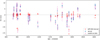 |
Fig. F.1 Comparison between HARPS-N RVs measured with the HARPS-N DRS from CCFs (open red circles) and with serval (open green circles). The red crosses show the difference between the two data-sets. The five points in which this difference is significantly negative correspond to exposures that were prematurely terminated, and which are not correctly processed by DRS. Both data-sets have been averaged to zero without considering these five points. The difference between the two data-sets has a standard deviation of 0.92 m s−1 (excluding again these five points). |
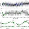 |
Fig. F.2 Like Fig. 13, but for Model 3 with the additional fit for a Keplerian signal with the lunar synodic period (29.53d). The lower left panel is again for the transiting planet b, while the lower right panel shows the RVs folded over the period of the additional signal. A similar plot for Model 2 does not show any relevant differences to the shown one. |
References
- Ahuir, J., Strugarek, A., Brun, A. S., & Mathis, S. 2021, A&A, 650, A126 [NASA ADS] [CrossRef] [EDP Sciences] [Google Scholar]
- Allard, F., Homeier, D., & Freytag, B. 2012, Philos. Trans. Roy. Soc. Lond. A, 370, 2765 [NASA ADS] [Google Scholar]
- Angus, R., Aigrain, S., Foreman-Mackey, D., & McQuillan, A. 2015, MNRAS, 450, 1787 [Google Scholar]
- Angus, R., Morton, T. D., Foreman-Mackey, D., et al. 2019, AJ, 158, 173 [Google Scholar]
- Attia, O., Bourrier, V., Eggenberger, P., et al. 2021, A&A, 647, A40 [EDP Sciences] [Google Scholar]
- Baranne, A., Queloz, D., Mayor, M., et al. 1996, A&AS, 119, 373 [NASA ADS] [CrossRef] [EDP Sciences] [Google Scholar]
- Barnes, S. A. 2007, ApJ, 669, 1167 [Google Scholar]
- Barragán, O., Gandolfi, D., & Antoniciello, G. 2019, MNRAS, 482, 1017 [Google Scholar]
- Barragán, O., Aigrain, S., Rajpaul, V. M., & Zicher, N. 2022, MNRAS, 509, 866 [Google Scholar]
- Bluhm, P., Luque, R., Espinoza, N., et al. 2020, A&A, 639, A132 [NASA ADS] [CrossRef] [EDP Sciences] [Google Scholar]
- Borucki, W. J., Koch, D., Basri, G., et al. 2010, Science, 327, 977 [Google Scholar]
- Bressan, A., Marigo, P., Girardi, L., et al. 2012, MNRAS, 427, 127 [NASA ADS] [CrossRef] [Google Scholar]
- Brown, T. M., Baliber, N., Bianco, F. B., et al. 2013, PASP, 125, 1031 [Google Scholar]
- Cabrera, J., Csizmadia, S., Erikson, A., Rauer, H., & Kirste, S. 2012, A&A, 548, A44 [NASA ADS] [CrossRef] [EDP Sciences] [Google Scholar]
- Cale, B., Plavchan, P., LeBrun, D., et al. 2019, AJ, 158, 170 [Google Scholar]
- Cannon, A. J., & Pickering, E. C. 1901, Ann. Harvard Coll. Observ., 28, 129 [NASA ADS] [Google Scholar]
- Castelli, F., & Kurucz, R. L. 2003, IAU Symp. 210, poster A20 [Google Scholar]
- Ceillier, T., van Saders, J., García, R. A., et al. 2016, MNRAS, 456, 119 [Google Scholar]
- Ceillier, T., Tayar, J., Mathur, S., et al. 2017, A&A, 605, A111 [NASA ADS] [CrossRef] [EDP Sciences] [Google Scholar]
- Chen, J., & Kipping, D. 2017, ApJ, 834, 17 [Google Scholar]
- Choi, J., Dotter, A., Conroy, C., et al. 2016, ApJ, 823, 102 [Google Scholar]
- Ciardi, D. R., Beichman, C. A., Horch, E. P., & Howell, S. B. 2015, ApJ, 805, 16 [NASA ADS] [CrossRef] [Google Scholar]
- Claret, A. 2017, A&A, 600, A30 [NASA ADS] [CrossRef] [EDP Sciences] [Google Scholar]
- Collins, K. 2019, in AAS Meeting Abstracts, 233, 140.05 [Google Scholar]
- Collins, K. A., Kielkopf, J. F., Stassun, K. G., & Hessman, F. V. 2017, AJ, 153, 77 [Google Scholar]
- Cosentino, R., Lovis, C., Pepe, F., et al. 2012, SPIE Conf. Ser., 8446, 84461V [Google Scholar]
- Cosentino, R., Lovis, C., Pepe, F., et al. 2014, SPIE Conf. Ser., 9147, 91478C [Google Scholar]
- Cowan, N. B., & Agol, E. 2011, ApJ, 729, 54 [Google Scholar]
- Dai, F., Masuda, K., & Winn, J. N. 2018, ApJ, 864, L38 [NASA ADS] [CrossRef] [Google Scholar]
- Dai, F., Masuda, K., Winn, J. N., & Zeng, L. 2019, ApJ, 883, 79 [NASA ADS] [CrossRef] [Google Scholar]
- da Silva, L., Girardi, L., Pasquini, L., et al. 2006, A&A, 458, 609 [NASA ADS] [CrossRef] [EDP Sciences] [Google Scholar]
- Dawson, R. I., & Fabrycky, D. C. 2010, ApJ, 722, 937 [Google Scholar]
- Deeg, H. J. 2014, Astrophysics Source Code Library [record ascl:1412.003] [Google Scholar]
- Dekany, R., Roberts, J., Burruss, R., et al. 2013, ApJ, 776, 130 [CrossRef] [Google Scholar]
- Díaz, M. R., Jenkins, J. S., Tuomi, M., et al. 2018, AJ, 155, 126 [CrossRef] [Google Scholar]
- Dorn, C., & Lichtenberg, T. 2021, ApJ, 922, L4 [NASA ADS] [CrossRef] [Google Scholar]
- Eastman, J., Gaudi, B. S., & Agol, E. 2013, PASP, 125, 83 [Google Scholar]
- Eastman, J. D., Rodriguez, J. E., Agol, E., et al. 2019, ArXiv e-prints [arXiv:1907.09480] [Google Scholar]
- Feng, F., Tuomi, M., & Jones, H. R. A. 2017, MNRAS, 470, 4794 [NASA ADS] [CrossRef] [Google Scholar]
- Ford, E. B. 2006, ApJ, 642, 505 [Google Scholar]
- Fossati, L., Erkaev, N. V., Lammer, H., et al. 2017, A&A, 598, A90 [NASA ADS] [CrossRef] [EDP Sciences] [Google Scholar]
- Frémat, Y., Royer, F., Marchal, O., et al. 2023, A&A, 674, A8 [NASA ADS] [CrossRef] [EDP Sciences] [Google Scholar]
- Fulton, B. J., Weiss, L. M., Sinukoff, E., et al. 2015, ApJ, 805, 175 [NASA ADS] [CrossRef] [Google Scholar]
- Fulton, B. J., Petigura, E. A., Howard, A. W., et al. 2017, AJ, 154, 109 [Google Scholar]
- Furlan, E., Ciardi, D. R., Everett, M. E., et al. 2017, AJ, 153, 71 [NASA ADS] [CrossRef] [Google Scholar]
- Gaia Collaboration (Brown, A.G.A., et al.) 2020, VizieR Online Data Catalog: I/350 [Google Scholar]
- García, R. A., Ceillier, T., Salabert, D., et al. 2014a, A&A, 572, A34 [NASA ADS] [CrossRef] [EDP Sciences] [Google Scholar]
- García, R. A., Mathur, S., Pires, S., et al. 2014b, A&A, 568, A10 [Google Scholar]
- García, R. A., Mathur, S., González Otero, J., Santos, A. R. G., & Breton, S. N. 2021, in Posters from the TESS Science Conference II (TSC2), 180 [Google Scholar]
- Gray, D. F. 2018, ApJ, 857, 139 [NASA ADS] [CrossRef] [Google Scholar]
- Gregory, P. C. 2005, ApJ, 631, 1198 [NASA ADS] [CrossRef] [Google Scholar]
- Hatzes, A. P. 2014, A&A, 568, A84 [NASA ADS] [CrossRef] [EDP Sciences] [Google Scholar]
- Hatzes, A. P., Dvorak, R., Wuchterl, G., et al. 2010, A&A, 520, A93 [NASA ADS] [CrossRef] [EDP Sciences] [Google Scholar]
- Hayward, T. L., Brandl, B., Pirger, B., et al. 2001, PASP, 113, 105 [NASA ADS] [CrossRef] [Google Scholar]
- Henden, A. A., Templeton, M., Terrell, D., et al. 2016, VizieR Online Data Catalog: II/336 [Google Scholar]
- Hippke, M., & Heller, R. 2019, A&A, 623, A39 [NASA ADS] [CrossRef] [EDP Sciences] [Google Scholar]
- Hofmann, H., Kafadar, K., & Wickham, H. 2011, Letter-value plots: Boxplots for large data, Tech. rep., had.co.nz [Google Scholar]
- Høg, E., Fabricius, C., Makarov, V. V., et al. 2000, A&A, 355, A27 [NASA ADS] [Google Scholar]
- Howard, A. W., Johnson, J. A., Marcy, G. W., et al. 2010, ApJ, 721, 1467 [Google Scholar]
- Husser, T. O., Wende-von Berg, S., Dreizler, S., et al. 2013, A&A, 553, A6 [NASA ADS] [CrossRef] [EDP Sciences] [Google Scholar]
- Hut, P. 1980, A&A, 92, 167 [NASA ADS] [Google Scholar]
- Ikoma, M., & Genda, H. 2006, ApJ, 648, 696 [NASA ADS] [CrossRef] [Google Scholar]
- Jenkins, J. M., Caldwell, D. A., Chandrasekaran, H., et al. 2010, ApJ, 713, L87 [Google Scholar]
- Jenkins, J. M., Twicken, J. D., McCauliff, S., et al. 2016, in Proc. SPIE, 9913, Software and Cyberinfrastructure for Astronomy IV, 99133E [Google Scholar]
- Kaminski, A., Trifonov, T., Caballero, J. A., et al. 2018, A&A, 618, A115 [NASA ADS] [CrossRef] [EDP Sciences] [Google Scholar]
- Kempton, E. M. R., Bean, J. L., Louie, D. R., et al. 2018, PASP, 130, 114401 [Google Scholar]
- Kilic, M., Munn, J. A., Harris, H. C., et al. 2017, ApJ, 837, 162 [Google Scholar]
- Kipping, D. M. 2013, MNRAS, 435, 2152 [Google Scholar]
- Kite, E. S., & Schaefer, L. 2021, ApJ, 909, L22 [NASA ADS] [CrossRef] [Google Scholar]
- Kite, E. S., Fegley, Bruce, J., Schaefer, L., & Ford, E.B. 2020, ApJ, 891, 111 [NASA ADS] [CrossRef] [Google Scholar]
- Kurucz, R. L. 1993, VizieR Online Data Catalog: VI/39 [Google Scholar]
- Kurucz, R. L. 2013, Astrophysics Source Code Library [record ascl:1303.024] [Google Scholar]
- Lafarga, M., Ribas, I., Lovis, C., et al. 2020, A&A, 636, A36 [NASA ADS] [CrossRef] [EDP Sciences] [Google Scholar]
- Lanza, A. F. 2021, A&A, 653, A112 [NASA ADS] [CrossRef] [EDP Sciences] [Google Scholar]
- Lee, E. J., & Chiang, E. 2017, ApJ, 842, 40 [Google Scholar]
- Lucy, L. B. 2013, A&A, 551, A47 [NASA ADS] [CrossRef] [EDP Sciences] [Google Scholar]
- Mamajek, E. E., & Hillenbrand, L. A. 2008, ApJ, 687, 1264 [Google Scholar]
- Mandel, K., & Agol, E. 2002, ApJ, 580, L171 [Google Scholar]
- Mathur, S., García, R. A., Régulo, C., et al. 2010, A&A, 511, A46 [NASA ADS] [CrossRef] [EDP Sciences] [Google Scholar]
- Mathur, S., García, R. A., Ballot, J., et al. 2014, A&A, 562, A124 [NASA ADS] [CrossRef] [EDP Sciences] [Google Scholar]
- Mazeh, T., Holczer, T., & Faigler, S. 2016, A&A, 589, A75 [NASA ADS] [CrossRef] [EDP Sciences] [Google Scholar]
- McCully, C., Volgenau, N. H., Harbeck, D.-R., et al. 2018, SPIE Conf. Ser., 10707, 107070K [Google Scholar]
- McQuillan, A., Aigrain, S., & Mazeh, T. 2013, MNRAS, 432, 1203 [Google Scholar]
- McQuillan, A., Mazeh, T., & Aigrain, S. 2014, ApJS, 211, 24 [Google Scholar]
- Mordasini, C., Alibert, Y., Georgy, C., et al. 2012, A&A, 547, A112 [NASA ADS] [CrossRef] [EDP Sciences] [Google Scholar]
- Mortier, A., & Collier Cameron, A. 2017, A&A, 601, A110 [NASA ADS] [CrossRef] [EDP Sciences] [Google Scholar]
- Mortier, A., Faria, J. P., Correia, C. M., Santerne, A., & Santos, N. C. 2015, A&A, 573, A101 [NASA ADS] [CrossRef] [EDP Sciences] [Google Scholar]
- Morton, T. D. 2015, Astrophysics Source Code Library [record ascl:1503.010] [Google Scholar]
- Murgas, F., Nowak, G., Masseron, T., et al. 2022, A&A, 668, A158 [NASA ADS] [CrossRef] [EDP Sciences] [Google Scholar]
- Narita, N., Fukui, A., Kusakabe, N., et al. 2019, J. Astron. Telescopes Instrum. Syst., 5, 015001 [Google Scholar]
- Papale, P. 1997, Contrib. Mineral. Petrol., 126, 237 [NASA ADS] [CrossRef] [Google Scholar]
- Parviainen, H., Tingley, B., Deeg, H. J., et al. 2019, A&A, 630, A89 [NASA ADS] [CrossRef] [EDP Sciences] [Google Scholar]
- Petigura, E. A., Rogers, J. G., Isaacson, H., et al. 2022, AJ, 163, 179 [NASA ADS] [CrossRef] [Google Scholar]
- Petrovich, C., Deibert, E., & Wu, Y. 2019, AJ, 157, 180 [NASA ADS] [CrossRef] [Google Scholar]
- Piskunov, N., & Valenti, J. A. 2017, A&A, 597, A16 [NASA ADS] [CrossRef] [EDP Sciences] [Google Scholar]
- Pu, B., & Lai, D. 2019, MNRAS, 488, 3568 [NASA ADS] [CrossRef] [Google Scholar]
- Quirrenbach, A., Amado, P. J., Caballero, J. A., et al. 2014, SPIE Conf. Ser., 9147, 91471F [Google Scholar]
- Quirrenbach, A., Amado, P. J., Ribas, I., et al. 2018, SPIE Conf. Ser., 10702, 107020W [Google Scholar]
- Rajpaul, V., Aigrain, S., Osborne, M. A., Reece, S., & Roberts, S. 2015, MNRAS, 452, 2269 [Google Scholar]
- Rayner, J., Tokunaga, A., Jaffe, D., et al. 2022, PASP, 134, 015002 [NASA ADS] [CrossRef] [Google Scholar]
- Reddy, B. E., Lambert, D. L., & Allende Prieto, C. 2006, MNRAS, 367, 1329 [Google Scholar]
- Rhodes, B. 2019, Astrophysics Source Code Library [record ascl:1907.024] [Google Scholar]
- Ricker, G. R., Winn, J. N., Vanderspek, R., et al. 2015, J. Astron. Telescopes Instrum. Syst., 1, 014003 [Google Scholar]
- Roberts, D. H., Lehar, J., & Dreher, J. W. 1987, AJ, 93, 968 [Google Scholar]
- Rodrigues, T. S., Girardi, L., Miglio, A., et al. 2014, MNRAS, 445, 2758 [Google Scholar]
- Rodrigues, T. S., Bossini, D., Miglio, A., et al. 2017, MNRAS, 467, 1433 [NASA ADS] [Google Scholar]
- Ryabchikova, T., Piskunov, N., Kurucz, R. L., et al. 2015, Phys. Scr, 90, 054005 [Google Scholar]
- Sanchis-Ojeda, R., Rappaport, S., Winn, J. N., et al. 2014, ApJ, 787, 47 [Google Scholar]
- Santos, N. C., Mortier, A., Faria, J. P., et al. 2014, A&A, 566, A35 [NASA ADS] [CrossRef] [EDP Sciences] [Google Scholar]
- Santos, A. R. G., García, R. A., Mathur, S., et al. 2019, ApJS, 244, 21 [Google Scholar]
- Santos, A. R. G., Breton, S. N., Mathur, S., & García, R. A. 2021, ApJS, 255, 17 [NASA ADS] [CrossRef] [Google Scholar]
- Sasaki, S. 1990, in Origin of the Earth, eds. H.E. Newson, & J.H. Jones (New York: Oxford Univ. Press), 195 [Google Scholar]
- Schlafly, E. F., & Finkbeiner, D. P. 2011, ApJ, 737, 103 [Google Scholar]
- Schlegel, D. J., Finkbeiner, D. P., & Davis, M. 1998, ApJ, 500, 525 [Google Scholar]
- Seager, S., Kuchner, M., Hier-Majumder, C. A., & Militzer, B. 2007, ApJ, 669, 1279 [NASA ADS] [CrossRef] [Google Scholar]
- Skrutskie, M. F., Cutri, R. M., Stiening, R., et al. 2006, AJ, 131, 1163 [NASA ADS] [CrossRef] [Google Scholar]
- Smith, J. C., Stumpe, M. C., Van Cleve, J. E., et al. 2012, PASP, 124, 1000 [Google Scholar]
- Smith, J. C., Stumpe, M. C., Jenkins, J. M., et al. 2020a, Kepler Data Processing Handbook: Presearch Data Conditioning, ed. J.M. Jenkins (Kepler Science Document KSCI-19081-003), 8 [Google Scholar]
- Smith, J. C., Stumpe, M. C., Jenkins, J. M., et al. 2020b, in Kepler Data Processing Handbook, ed. J. Jenkins (NASA, Kepler Science Document KSCI-19081-003), 131 [Google Scholar]
- Spada, F., & Lanzafame, A. C. 2020, A&A, 636, A76 [NASA ADS] [CrossRef] [EDP Sciences] [Google Scholar]
- Stassun, K. G., Oelkers, R. J., Pepper, J., et al. 2018, AJ, 156, 102 [Google Scholar]
- Stassun, K. G., Oelkers, R. J., Paegert, M., et al. 2019, AJ, 158, 138 [Google Scholar]
- Strugarek, A. 2016, ApJ, 833, 140 [NASA ADS] [CrossRef] [Google Scholar]
- Stumpe, M. C., Smith, J. C., Van Cleve, J. E., et al. 2012, PASP, 124, 985 [Google Scholar]
- Stumpe, M. C., Smith, J. C., Catanzarite, J. H., et al. 2014, PASP, 126, 100 [Google Scholar]
- Suissa, G., Chen, J., & Kipping, D. 2018, MNRAS, 476, 2613 [Google Scholar]
- Tenenbaum, P., & Jenkins, J.M. 2018, TESS Science Data Products Description Document EXP-TESS-ARC-ICD-0014 Rev D (Moffet Field, California: NASA Ames Research Center) [Google Scholar]
- Ter Braak, C. J. F. 2006, Stat. Comput., 16, 239 [Google Scholar]
- Torrence, C., & Compo, G. P. 1998, Bull. Am. Meteorol. Soc., 79, 61 [Google Scholar]
- Torres, G. 2010, AJ, 140, 1158 [Google Scholar]
- Trifonov, T., Kürster, M., Zechmeister, M., et al. 2018, A&A, 609, A117 [NASA ADS] [CrossRef] [EDP Sciences] [Google Scholar]
- Turbet, M., Bolmont, E., Ehrenreich, D., et al. 2020, A&A, 638, A41 [NASA ADS] [CrossRef] [EDP Sciences] [Google Scholar]
- Twicken, J. D., Catanzarite, J. H., Clarke, B. D., et al. 2018, PASP, 130, 064502 [Google Scholar]
- Valenti, J. A., & Piskunov, N. 1996, A&AS, 118, 595 [NASA ADS] [CrossRef] [EDP Sciences] [Google Scholar]
- Van Eylen, V., Agentoft, C., Lundkvist, M. S., et al. 2018, MNRAS, 479, 4786 [Google Scholar]
- Vines, J. I., & Jenkins, J. S. 2022, MNRAS, 513, 2719 [NASA ADS] [CrossRef] [Google Scholar]
- Vogt, S. S., Allen, S. L., Bigelow, B. C., et al. 1994, SPIE Conf. Ser., 2198, 362 [NASA ADS] [Google Scholar]
- Vogt, S. S., Radovan, M., Kibrick, R., et al. 2014, PASP, 126, 359 [NASA ADS] [CrossRef] [Google Scholar]
- Winn, J. N., Sanchis-Ojeda, R., & Rappaport, S. 2018, New A Rev., 83, 37 [Google Scholar]
- Yee, S. W., Petigura, E. A., & von Braun, K. 2017, ApJ, 836, 77 [Google Scholar]
- Zechmeister, M., Reiners, A., Amado, P. J., et al. 2018, A&A, 609, A12 [NASA ADS] [CrossRef] [EDP Sciences] [Google Scholar]
- Zeng, L., & Jacobsen, S. B. 2017, ApJ, 837, 164 [NASA ADS] [CrossRef] [Google Scholar]
- Zeng, L., & Sasselov, D. 2013, PASP, 125, 227 [Google Scholar]
- Zeng, L., Sasselov, D. D., & Jacobsen, S. B. 2016, ApJ, 819, 127 [Google Scholar]
- Zeng, L., Jacobsen, S. B., Sasselov, D. D., et al. 2019, PNAS, 116, 9723 [Google Scholar]
Retrieved from the NASA Exoplanet Archive in February 2023.
These values are from the Data Validation Report Summary of TOI 1416.01 for the combined S14, S23 and S50 data, available at MAST (https://mast.stsci.edu) as file tess2019199201929-s0014-s0050-0000000150025009-00611_dvm.pdf.
Cadences of expected low quality are identified by a bit-wise AND of the quality flag of a given data point with the binary number 0101001010111111, as recommended in the TESS Archive Manual at https://outerspace.stsci.edu/display/TESS/2.0+-+Data+Product+Overview
The contamination ratio cTIC is defined as the ratio of flux from nearby objects that falls in the aperture of the target star, divided by the target star flux in the aperture (Stassun et al. 2018).
CROWDSAP is defined as the ratio of the flux from the target to the total flux in the aperture (Tenenbaum & Jenkins 2018). A conversion is therefore given by CROWDSAP = 1/(1 + cTIC).
Available at http://ia2-harps.oats.inaf.it:8000
The figures were generated with the latest version of the code for the BGLS and related plots, available from A. Mortier in https://anneliesmortier.wordpress.com/sbgls/
Available at https://github.com/oscaribv/pyaneti
The quoted range of water mass-fractions was derived from interpolation within Fig. 4 of Dorn & Lichtenberg (2021), considering the mass and radius uncertainties of TOI-1416 b.
Kempton et al. (2018) give a suggested cutoff of 92 in their Table 1, but we note that TOI-1416 b’s radius of 1.6 R⊕ is near the lower limit of their 1.5 < Rp < 2.75 R⊕ radius bin.
We note that the limits for the Neptune Desert given by Mazeh et al. (2016) do not attempt to delineate an area that is empty of planets, but rather they were placed to produce the best contrast between the lower-density ‘desert’ and its more densely populated surroundings.
We note that the bump at 1 day in Lee & Chiang (2017) might be a result from the integration of two different studies, one for period of less than 1 day, and one for periods larger than 1 day, with different stellar host types.
Assuming a spectral line broadening of TOI-1416 of 7.0 ± 1.7 km/s (Gaia DR3; see also Frémat et al. 2023) and of the Sun of ≈5.6 km/s (Gray 2018, sum of rotational broadening and macro-turbulence).
The skyfield python package (Rhodes 2019) was used to calculate all values related to the Moon’s position or velocity at the time of the observations
The Keplerian signal corresponding to planet b was subtracted from these RVs. However, the presence or absence of the planet b signal does not alter the shown plots and the conclusions in any relevant way.
We also note that the three outliers near the lunar phase of 200° in Fig. B.3 agree now well with the other RVs; these were taken in twilight when a nearly full Moon was just below horizon
UTM/UFIT version 8mar22 was used for most of the work described; its latest version is available at https://github.com/hdeeg/utm_ufit/
Preprocessor modules (provided in the software distribution or userdefined ones) are used to convert the input parameters into the basic set of system parameters used internally by UTM
The stellar density was mainly chosen for compatibility with the fixed set of input parameters used by pyaneti, described in Sect. 5.2. A preprocessor routine to UTM converts the stellar density into the usually used ratio of the semimajor axis versus the stellar radius, ap/R⋆, using, e.g., Eq. (31) of Barragán et al. (2019).
All Tables
Spectroscopic parameters for TOI-1416 derived with SME and SpecMatch-Emp and comparison values from Gaia and the TIC.
Stellar masses and radii with corresponding mean densities of TOI-1416 derived with different models with priors from SME.
Priors and inferred parameters from transit and RV modeling with pyaneti (Model 3) and UTM/UFIT or FCO.
All Figures
|
Fig. 1 Phased light curve around the transits of TOI-1416 b. Black crosses represent the TESS light curve, after phasing by the planet’s period against the adopted ephemeris and the correction against gradients in the off-transit sections, as described in Sect. 2. Green crosses represent the same curve after a box-car smoothing over 100 phased data points and posterior binning over 50 points. We note that the average time increment between the binned points is 126 seconds, which is very similar to the 120 s temporal resolution of TESS light curves. The red curve is the transit model generated with UTM/UFIT, described in Appendix C. The vertical dashed orange lines indicate the limits between the on-transit and off-transit sections. |
| In the text | |
|
Fig. 2 O-C diagram of the transit epochs of TESS Sectors 16, 23, and 50, against the adopted ephemeris (dotted black line). |
| In the text | |
|
Fig. 3 Relative RVs of TOI-1416 from all contributing instruments. Each instrument’s set of RVs was offset separately to an average of zero. |
| In the text | |
|
Fig. 4 Full field of view image of the final combined dither pattern for the Palomar AO imaging. |
| In the text | |
|
Fig. 5 Companion sensitivity for the Palomar AO imaging. The black points represent the 5σ limits and are separated in steps of 1 FWHM (≈0.1″); the purple zone represents the azimuthal dispersion (lσ) of the contrast determinations (see the main text). The inset image is of the primary target and shows no additional companions within 3″ of the target. |
| In the text | |
|
Fig. 6 Time series of a predicted transit of TOI-1416 b on March 08, 2021 UT, observed by the LCOGT. The gray dots are the unbinned differential photometry (no detrending applied), and the green dots show the data in 10-min bins. The green line is a transit-model fit to the data using priors from the Data Validation Report mentioned in Sect. 2, except for the epoch and the size of the planet, which were unconstrained parameters. |
| In the text | |
|
Fig. 7 SED of TOI-1416. The best fitting model from the Phoenix v2 grids is shown in black. The observed photometry is marked with cyan circles, and the synthetic photometry with magenta diamonds. The horizontal bars of the observations indicate the effective widths of the passbands, while the vertical bars mark the 1 σ uncertainties. The lower panel shows the residuals normalized to the errors of the photometry, which causes the most precise photometry to display the largest scatter. |
| In the text | |
|
Fig. 8 Co-added HARPS-N spectrum of TOI-1416 in the range of the Ca H & K lines (arrows), with zoomed-in views (lower panels) around the Ca K (3933.66 Å) and Ca H (3968.47 Å) lines. |
| In the text | |
|
Fig. 9 BGLS periodograms of the HARPS-N observations, for the measured RVs and for several activity indicators. The vertical scale is given in units of the logarithm of the Bayesian probability of a signal with a given period, where the highest peak is normalized to log p = 0. The lowest panel shows the spectral window function of the sampled data. See also Figs. 10 and B.1 for zoomed-in views around the 1.07 days and 29.5 days periods of planet b and the candidate c, respectively. |
| In the text | |
|
Fig. 10 Zoomed-in view of the BGLS periodogram of Fig. 9, around the 1.07 days period of the transiting planet, b, where only a minor peak is discernible in the RVs (top panel). The highest RV peaks at P = 1.035 days and P = 0.967 days are aliases of the 29.5 days signal over the sample period of the solar or the sidereal day. Their periods of 1.0 and 0.9973 days show up as the principal double peak in the window function (lowest panel). |
| In the text | |
|
Fig. 11 Left panel: Bayes factor periodogram of the HARPS-N RVs generated by agatha (Feng et al. 2017), using one MA component. The vertical axis provides the probability of peaks being real, in terms of the logarithm of their Bayes factor (BF). The period of the highest peak is indicated, which corresponds to the period of the transits of TOI-1416 b. Right panel: Like the left panel, but after the removal of the 1.069 days signal, now showing a signal at 29.52 days as the highest one. |
| In the text | |
|
Fig. 12 Correlations in the HARPS-N data between the RVs (labeled as RV_srv and the activity indicators listed in Sect. 3.1.2. The Pearson correlation coefficient is indicated in each panel. |
| In the text | |
|
Fig. 13 Modeling of HARPS-N spectroscopy with pyaneti. Upper panel: RV and dLW time series for Model 1, assuming only the presence of a Keplerian signal with the 1.07 days transit period. The green markers in each panel represent the RV and dLW measurements. The solid black curve shows the inferred multi-GP model, with dark and light shaded areas showing the one and two sigma credible intervals of the corresponding GP model. We note that the short period of the planet and the size of the plot make the RV sinusoids appear as a solid blue band. Lower panel: HARPS-N RV data folded on the 1.07-day orbital period of planet b, after subtraction of the systemic velocity and the GP noise model. The inferred RV model is shown as a solid black curve with 1- and 2-sigma credible intervals (shaded areas). |
| In the text | |
|
Fig. 14 Planet masses and radii, versus composition models: Gray markers indicate planets with well-determined masses (errors smaller than 30%, from adopted values in the NASA Exoplanet Archive). Planets with periods of less than 2 days are shown with brown markers. Composition models indicated by solid lines are from Zeng et al. (2016, 2019), whereas the dashed line is a model from Dorn & Lichtenberg (2021) for an Earth-like rocky composition (66% Mg-Si oxides and silicates and 33% iron), where the molten rock contains water with a mass fraction of 5.4%. TOI-1416 b is indicated by the red dot. |
| In the text | |
|
Fig. 15 Like Fig. 14, but in mass-density space, with the density given relative to the Earth’s density of 5.51 g cm−3. |
| In the text | |
|
Fig. 16 Diagram of the radii (top panel) and. masses (bottom panel) versus period of the known planets, from the NASA Exoplanet Archive. The solid black lines show the delineation of the “Neptune Desert” from Mazeh et al. (2016), whereas the horizontal dotted black lines show the lower limits to the Neptune Desert for periods ≤2 days that are proposed in this work. The dashed orange line in the upper panel indicates the period-radius valley from Van Eylen et al. (2018). TOI-1416 b is indicated by the filled red circle and the tentative planet c by the unfilled one. |
| In the text | |
|
Fig. 17 Distributions of small planets of log R/R⊕ < 0.8 (or R/R⊕ < 6.3) and with periods shorter than 3.6 days, after categorizing their population into bins with a width of log P(day) = 0.125. Top panel: Distribution of planet radii against the orbital period. The distributions are shown as “boxenplots” or “letter value plots” (Hofmann et al. 2011). TOI-1416 b is indicated by the red star. Bottom panel: Counts of the small planets versus the same bins in orbital period. |
| In the text | |
|
Fig. A.1 Analysis of TESS light curve for stellar rotation of TOI-1416. The top panel shows the light curve from Sector 16 and 23 that was used for the analysis. The following panels show the three methods used for the period determination (see the main text): the GWPS and its projection onto the period axis; the ACF; and the composite spectrum (CS). The hatched region in the panel for the GWPS indicates the zone where the method is not valid. |
| In the text | |
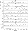 |
Fig. B.1 Zoomed-in view of the BGLS periodogram of Fig. 9, around the 29.5 d period of planet c. |
| In the text | |
|
Fig. B.2 Observed uncorrected RVs of TOI-1416 versus calculated RVs of the Moon-reflected solar spectrum. The symbol colors indicate if the Moon was above (pink) or below the horizon (blue) at the moment of observation. The green line corresponds to identical RV values on both axes. |
| In the text | |
|
Fig. B.3 HARPS-N RVs folded against the lunar phase, where 0° or 360° corresponds to New Moon and 180° to Full Moon. The clumping of the RV data in two regions of lunar phases, with an avoidance of Full Moon and lesser coverage near New Moon, is a consequence of the scheduling of the HARPS-N observations, which were mostly executed in lunar gray time. |
| In the text | |
|
Fig. B.4 Similar to Fig. B.3, but the HARPS-N RVs are plotted against the lunar illumination at the time of observation, and the data are separated into panels containing only RVs that were taken when the Moon was below or above the horizon. The blue line in the right panel shows a linear fit to the RV versus illumination dependence, which has a correlation coefficient of −0.69. |
| In the text | |
|
Fig. B.5 BGLS periodograms of the HARPS-N RVs and window functions, with the RV data separated into those taken when the Moon was below and above the horizon. The blue numbers indicate the number of RV points. |
| In the text | |
|
Fig. B.6 BGLS periodograms of the RVs of the contributing instruments. In the left column are those that show a peak near 27 or 29 days (vertical red lines); in the center are those that do not. The right panel shows a periodogram with the RVs from all instruments combined. The blue numbers indicate the number of RVs used. |
| In the text | |
|
Fig. B.7 Development of the S/N (black curves) and the best-fitting amplitude “bestK” (blue curves, in m/s) of RV signals with periods of 27.40 d (top set of panels) and 29.53 d (bottom set), versus the number of RV points since the first measurement. The left panels are based on RVs from HARPS-N and the right ones on RVs from the APF. |
| In the text | |
|
Fig. C.1 Graphical output from MCMC sequence performed by UFIT that led to the results reported in Table 7. In all panels, the parameters are indicated by the keywords used in UFIT: “1period” for the planet period, “1trepoch” for the epoch of transit, “1radi” for the relative planet radius, “0densCGS” for the stellar density in CGS units, “1impact” for the impact parameter, “0limbd” and “0limbd2” for the LD coefficients q1 and q2, and “ooff” for the off-transit flux-offset against zero. The sub-figures are: (a) Values of the parameters against link-number of the MCMC sequence, excluding burn-in. Each MCMC chain is shown by a different color. The lowest panel shows the evaluation of the χ2 values. (b) Scatter plot of parameters versus the χ2 value. (c) Histograms of parameter distributions. The median value is shown by the vertical black line; the dashed lines delimit the 68.3% credible interval and the red line gives the value of the best fit. (d) Corner plot of the correlations among parameters. The red crosses give the values of the best fit. |
| In the text | |
|
Fig. D.1 Best-fit χ2 from FCO fits of HARPS-N data to a series of RV models of TOI-1416 b with fixed RV-amplitudes K. |
| In the text | |
|
Fig. D.2 FCO fit to the HARPS-N RVs. Upper panel: Phase-folded RV model (green line) of TOI-1416 b, which corresponds to the best fit from the FCO method, obtained by vertically offsetting nightly chunks of RV data against the model. RV points from the same nights have identical colors. Lower panel: Small section of the RV model plotted against time, with RVs from three different nights. |
| In the text | |
|
Fig. E.1 Similar to Fig. 16, but with planet radii (top panel) and masses (bottom panel) plotted against the planets’ insolation (lower X-axis) and their effective temperature (upper X-axis). The solid black lines show the delineation of the Neptune Desert against insolation and Teff, whereas the horizontal dotted black lines show the same lower limits to the Neptune Desert as those proposed for periods of P ≲ 2d. The dashed orange line in the upper panel indicates the radius valley against insolation from Petigura et al. (2022). TOI-1416 b is indicated by the filled red circle and c by the unfilled one. |
| In the text | |
|
Fig. F.1 Comparison between HARPS-N RVs measured with the HARPS-N DRS from CCFs (open red circles) and with serval (open green circles). The red crosses show the difference between the two data-sets. The five points in which this difference is significantly negative correspond to exposures that were prematurely terminated, and which are not correctly processed by DRS. Both data-sets have been averaged to zero without considering these five points. The difference between the two data-sets has a standard deviation of 0.92 m s−1 (excluding again these five points). |
| In the text | |
|
Fig. F.2 Like Fig. 13, but for Model 3 with the additional fit for a Keplerian signal with the lunar synodic period (29.53d). The lower left panel is again for the transiting planet b, while the lower right panel shows the RVs folded over the period of the additional signal. A similar plot for Model 2 does not show any relevant differences to the shown one. |
| In the text | |
Current usage metrics show cumulative count of Article Views (full-text article views including HTML views, PDF and ePub downloads, according to the available data) and Abstracts Views on Vision4Press platform.
Data correspond to usage on the plateform after 2015. The current usage metrics is available 48-96 hours after online publication and is updated daily on week days.
Initial download of the metrics may take a while.