| Issue |
A&A
Volume 692, December 2024
|
|
|---|---|---|
| Article Number | A238 | |
| Number of page(s) | 22 | |
| Section | Planets, planetary systems, and small bodies | |
| DOI | https://doi.org/10.1051/0004-6361/202452244 | |
| Published online | 18 December 2024 | |
Characterisation of TOI-406 as a showcase of the THIRSTEE program
A two-planet system straddling the M-dwarf density gap
1
Instituto de Astrofísica de Canarias (IAC),
38205
La Laguna,
Tenerife,
Spain
2
Departamento de Astrofísica, Universidad de La Laguna (ULL),
38206
La Laguna,
Tenerife,
Spain
3
Department of Astronomy and Astrophysics, University of Chicago,
Chicago,
IL
60637,
USA
4
Institut Trottier de recherche sur les exoplanètes, Département de Physique, Université de Montréal,
Montréal,
Québec,
Canada
5
Department of Astronomy and Astrophysics, University of California,
Santa Cruz,
CA
95064,
USA
6
Centro de Astrobiología (CSIC-INTA),
Crta. Ajalvir km 4,
28850
Torrejón de Ardoz, Madrid,
Spain
7
Departamento de Física de la Tierra y Astrofísica & IPARCOS-UCM (Instituto de Física de Partículas y del Cosmos de la UCM), Facultad de Ciencias Físicas, Universidad Complutense de Madrid,
28040
Madrid,
Spain
8
Center for Astrophysics | Harvard & Smithsonian,
60 Garden Street,
Cambridge,
MA
02138,
USA
9
Observatoire du Mont-Mégantic, Université de Montréal,
C.P. 6128, Succ. Centre-ville,
Montréal
H3C 3J7,
Québec,
Canada
10
Institute of Astronomy, Faculty of Physics, Astronomy and Informatics, Nicolaus Copernicus University,
Grudziadzka 5,
87–100
Toruń,
Poland
11
Observatoire de Genève, Département d’Astronomie, Université de Genève,
Chemin Pegasi 51b,
1290
Versoix,
Switzerland
12
Departamento de Física Teórica e Experimental, Universidade Federal do Rio Grande do Norte, Campus Universitário,
Natal,
RN 59072-970,
Brazil
13
INAF – Osservatorio Astrofisico di Arcetri,
Largo E. Fermi 5,
Florence,
Italy
14
INAF – Osservatorio Astrofisico di Torino,
Via Osservatorio 20,
10025
Pino Torinese,
Italy
15
University of Grenoble Alpes, CNRS, IPAG,
F-38000
Grenoble,
France
16
American Association of Variable Star Observers,
185 Alewife Brook Parkway, Suite 410,
Cambridge,
MA
02138,
USA
17
Department of Physics & Astronomy, University of Kansas,
1082 Malott, 1251 Wescoe Hall Drive,
Lawrence,
KS 66045,
USA
18
The Maury Lewin Astronomical Observatory,
Glendora,
CA
91741,
USA
19
Light Bridges S.L., Observatorio del Teide,
Carretera del Observatorio, s/n Guimar,
38500
Tenerife,
Canarias,
Spain
20
University Observatory, Faculty of Physics, Ludwig-Maximilians-Universität München,
Scheinerstr. 1,
81679
Munich,
Germany
21
European Southern Observatory (ESO),
Karl-Schwarzschild-Str. 2,
85748
Garching bei München,
Germany
22
Kotizarovci Observatory,
Sarsoni 90,
51216
Viskovo,
Croatia
23
Mullard Space Science Laboratory, University College London,
Surrey,
UK
★ Corresponding author; glacedelli@iac.es
Received:
13
September
2024
Accepted:
2
November
2024
Context. The exoplanet sub-Neptune population currently poses a conundrum, as to whether small-size planets are volatile-rich cores without an atmosphere, or rocky cores surrounded by a H-He envelope. To test the different hypotheses from an observational point of view, a large sample of small-size planets with precise mass and radius measurements is the first necessary step. On top of that, much more information will likely be needed, including atmospheric characterisation and a demographic perspective on their bulk properties.
Aims. We present here the concept and strategy of the THIRSTEE project, which aims to shed light on the composition of the sub-Neptune population across stellar types by increasing their number and improving the accuracy of bulk density measurements, as well as investigating their atmospheres and performing statistical, demographic analysis. We report the first results of the program, characterising a new two-planet system around the M-dwarf TOI-406.
Methods. We analysed TESS and ground-based photometry together with high-precision ESPRESSO and NIRPS/HARPS radial velocities to derive the orbital parameters and investigate the internal composition of the two planets orbiting TOI-406.
Results. TOI-406 hosts two planets with radii and masses of Rc = 1.32 ± 0.12 R⊕, Mc = 2.08−0.22+0.23 M⊕ and Rb = 2.08−0.15+0.16 R⊕, Mb = 6.57−0.90+1.00 M⊕, orbiting with periods of 3.3 and 13.2 days, respectively. The inner planet is consistent with an Earth-like composition, while the external one is compatible with multiple internal composition models, including volatile-rich planets without H/He atmospheres. The two planets are located in two distinct regions in the mass-density diagram, supporting the existence of a density gap among small exoplanets around M dwarfs. With an equilibrium temperature of only Teq = 368 K, TOI-406 b stands up as a particularly interesting target for atmospheric characterisation with JWST in the low-temperature regime.
Key words: planets and satellites: composition / planets and satellites: detection / planets and satellites: individual: TOI-406
© The Authors 2024
 Open Access article, published by EDP Sciences, under the terms of the Creative Commons Attribution License (https://creativecommons.org/licenses/by/4.0), which permits unrestricted use, distribution, and reproduction in any medium, provided the original work is properly cited.
This article is published in open access under the Subscribe to Open model. Subscribe to A&A to support open access publication.
1 Introduction
The increasing number of discovered exoplanets, more than 5500 at present, now allows for the development of demographic studies based on the general properties of the observed planetary population. In the last few decades, space-based missions such as Kepler (Borucki et al. 2010) and, more recently, TESS (Ricker et al. 2014), have identified an emerging population of planets with sizes between the Earth and Neptune, also known as sub-Neptunes. This population of small-size planets (1 R⊕ < Rp < 4 R⊕) is absent in the Solar System, but more than half of all Sun-like stars in the Galaxy host a sub-Neptune interior to 1 AU (e.g. Batalha et al. 2013; Marcy et al. 2014b; Petigura et al. 2013). Thus, understanding the origin and nature of the sub-Neptune population is not only essential to inform our understanding of the planetary formation and evolution processes, but it also helps us to picture our Solar System in a global context.
The sub-Neptune population shows a paucity of planets with sizes between 1.5 and 2.0 R⊕, known as ‘radius gap’ (Fulton et al. 2017; Van Eylen et al. 2018; Hirano et al. 2018; Berger et al. 2020; Cloutier et al. 2020; Petigura et al. 2022), which sparked the development of planet formation and evolution models that could explain this observational feature. One of the most common interpretations is attributed to atmospheric evolution, which can reproduce the observed dependency of the gap location as a function of incident stellar irradiation, and the fact that most of the highly-irradiated sub-Neptunes have Earth-like densities (Dai et al. 2019). In this scenario, planets below the radius gap (known as super-Earths) are bare rocky cores that have been fully stripped from their primordial hydrogen-dominated atmosphere originally accreted from the protoplanetary disc. This atmospheric mass loss is mainly thought to be due to XUV radiation from young stars (Owen & Wu 2013; Lopez & Fortney 2013) or to the heat coming from cooling cores (Ginzburg et al. 2018; Gupta & Schlichting 2019), even though other mechanisms such as giant impacts have also been investigated (Wyatt et al. 2020). These atmospheric mass loss theories predict that planets above the gap (‘gas dwarfs’ hereafter - also known as mini-Neptunes) are Earth-like cores formed in the inner regions of the proto-planetary disc that retained their primordial atmospheres without being substantially enriched in volatiles (Ikoma & Hori 2012; Lee et al. 2014; Lee & Chiang 2016). Models that include in situ gas accretion during the gas-poor phase of disc evolution (Lee et al. 2022) are also able to reproduce the observations.
An alternative interpretation of the radius distribution of the sub-Neptune population is that super-Earths and mini-Neptunes are instead two different types of planets: the former consisting of a rock-iron mixture (a scaled-up version of Earth) and the latter consisting of a water-rock mixture (a scaled-up version of the Solar System’s icy moons), known as ‘water worlds’ (Léger et al. 2004; Rogers 2015; Mousis et al. 2020; Dorn & Lichtenberg 2021). Water worlds have intrinsically larger sizes with respect to super-Earths, due to their lower bulk density. In the water world hypothesis, planets formed beyond the ice line (or have been significantly polluted by pebbles or planetes-imals coming from that external region), and then migrated to the inner parts of the system (Raymond et al. 2018; Bitsch et al. 2019; Izidoro et al. 2022). While several fine-tuning effects must be introduced to replicate the properties of the gas dwarfs (Lee et al. 2014; Owen & Wu 2016; Liu et al. 2017; Kite et al. 2019; Esteves et al. 2020; Ogihara et al. 2020), water worlds are a natural outcome of formation and migration processes independent of the accretion mechanism (planetesimal or pebble) and the initial conditions of the protoplanetary disc (Raymond et al. 2018; Bitsch et al. 2019; Venturini et al. 2020; Burn et al. 2021; Izidoro et al. 2022). The same models are also able to reproduce the demographic features that originally favoured the gas dwarfs hypothesis, such as their large abundance (Mayor et al. 2011; Mulders et al. 2018), typical masses (Weiss & Marcy 2014; Otegi et al. 2020), radii (Fulton & Petigura 2018; Petigura et al. 2022), and period ratio and multiplicity distributions (Lissauer et al. 2011; Fabrycky et al. 2014). Moreover, various recent individual discoveries (Luque et al. 2021, 2022; Cadieux et al. 2022; Piaulet et al. 2023; Diamond-Lowe et al. 2022; Cherubim et al. 2023; Osborne et al. 2023; Cadieux et al. 2024a,b) have provided increasing evidence that such planets exist.
Recently, using a refined catalogue of small planets (Rp< 4 R⊕), Luque & Pallé (2022) proposed that for M dwarf hosts, the radius gap is a consequence of interior composition rather than an indicator of atmospheric mass loss. The authors show that M-dwarf planets seem to be distributed into three main populations: 1) planets that follow a bulk density comparable to the one of the Earth (e.g. rocky planets), 2) planets with cores consisting of a mixture of rock and water-dominated ices in a 50:50 mass proportion (e.g. water worlds), and 3) planets with a significant envelope made of H/He.
In this scenario, the apparent paucity of planets in the 1.5–2.0 R⊕ radius range is due to the combination of the rocky population reaching at most 10 M⊕, and the water world population having a minimum mass of 2–3 M⊕. The rock-ice proportion in the water world population identified in Luque & Pallé (2022) is not a coincidence, since internal structure models consistent with 50:50 admixtures of rock and water ices (Zeng et al. 2019; Mousis et al. 2020) perfectly match the ratio of rocky and volatile material measured beyond the ice line in protoplanetary discs (Lodders 2003) – even though the amount and storage mechanisms of water in planetary interiors is still debated (Dorn & Lichtenberg 2021; Vazan et al. 2022; Luo et al. 2024). Generally, water is not expected to be in condensed form for the known subNeptune population (typically close-in; hence, hot), but recent formation and evolution models that account for the effect of supercritical water mixed with H/He still reproduce the radius gap at the observed location (Burn et al. 2024).
However, this sub-Neptune population sits in a nexus of interior structure modelling degeneracy. Often, multiple combinations of interior compositions, including varying percentages of rocky and icy materials, and gases, can match the radius and mass measurements of individual planets (Rogers & Seager 2010), as well as the observed mass-radius trends, as is extensively explored in Parc et al. (2024). As an example, Rogers et al. (2023) show that the precise bulk densities of M-dwarf planets from Luque & Pallé (2022) can be also reproduced assuming a gas dwarf composition, if using atmospheric mass loss models that include spontaneous mass loss (also known as ‘boil-off’) after disc dispersal (Ikoma & Hori 2012; Owen & Wu 2016). The two scenarios (atmospheric mass loss, and the water-world hypothesis) are thus able to explain the individual and demographic properties of this population, highlighting the need for more detailed studies. This need for a large population of precisely characterised sub-Neptune planets is the subject of this paper, and of the THIRSTEE project.
This paper is organised as follows: in Sect. 2 we describe the rational and observational strategy of the THIRSTEE project, and in the rest of the work we present its first result; that is, the analysis and characterisation of a new planetary system around the M dwarf TOI-406 as part of the THIRSTEE sample. For the system characterisation, we used TESS (Sect. 3) and ground-based photometry together with two radial velocity (RV) datasets coming from ESPRESSO and NIRPS/HARPS, collected under the THIRSTEE project and the NIRPS Guaranteed Time Observations (GTO), respectively (Sect. 4). With these data, we precisely infer stellar parameters (Sect. 5) and mass, radius, and orbital configuration (Sect. 6) for the two planets orbiting TOI-406. We discuss our results and the potential of the THIRSTEE program using TOI-406 as a benchmark target within the context of the formation and evolution processes of the sub-Neptune population in Sect. 7.
2 THIRSTEE: Rationale and survey strategy
To investigate the origin and nature of sub-Neptunes, precise and accurate bulk density measurements are needed. Masses and radii are necessary to begin modelling their internal and atmospheric properties at an individual level and enable a demographic understanding of these planets as a population. Radial velocity follow-up of transiting exoplanets is the most extensive approach to measure the masses of these planets since, contrary to transit timing variations, it does not require the systems to be close to orbital resonance in order to characterise them. Despite the influence of stellar activity on multiple timescales, the incredibly precise ephemeris from transit observations (namely, the orbital period and phase of the planet) ease the modelling of the RV data, providing precise and accurate measurements of the planet masses in combination with stellar and instrumental mitigation strategies. The development of extremely precise RV instruments capable of sub-metre-per-second internal precision (e.g. ESPRESSO, MAROON-X, EXPRES, NEID, KPF, NIRPS) enables, in addition, the mass characterisation of transiting sub-Neptunes to be extended from low-mass stars (with typical RV semi-amplitudes of 1–2 m/s) to Sun-like stars (with typical RV semi-amplitudes of 30–70 cm/s).
To fill this gap, we have started the THIRSTEE1 survey. The core of THIRSTEE revolves around the following questions: whether sub-Neptunes are gas dwarfs or water worlds; whether water worlds exist only around M dwarfs or also around Sun-like stars; and, if both exist, what their relative occurrence is and how it depends on other system properties.
To tackle these questions, THIRSTEE takes an observational approach and, at the core of the project, is a dedicated RV survey to increase the number and improve the accuracy of bulk density measurements of transiting sub-Neptunes. We are particularly interested in extending the known sample in two important axes that have been largely unexplored: planet equilibrium temperature and host spectral type. The dependence on planet bulk density with host spectral type (as a proxy of stellar mass) contains the most information to connect the observed population with global models of planet formation and evolution (as recently highlighted by, e.g., Venturini et al. 2024; Chakrabarty & Mulders 2024). On the other hand, a sample of sub-Neptunes with ranging equilibrium temperatures and host spectral types is necessary to constrain the chemistry and interior structure of this population via atmospheric characterisation. Aerosol obfuscation has been proposed to explain the attenuated spectral features of sub-Neptune atmospheres in transmission as a function of equilibrium temperature (Brande et al. 2024). However, there is a degeneracy between clouds and high atmospheric mean molecular weight in feature amplitude that HST could not resolve. The first JWST observations of cool sub-Neptunes orbiting M dwarfs show that aerosols are not needed to explain their feature attenuation (Madhusudhan et al. 2023; Benneke et al. 2024; Piaulet-Ghorayeb et al. 2024). For JWST to break this degeneracy within its lifetime, a large sample of transiting sub-Neptunes with excellent observability metrics that spans a large range of planet equilibrium and stellar effective temperatures is needed. Besides, mass measurements are a prerequisite for atmospheric studies of small exoplanets to break degeneracies from atmospheric retrievals (Batalha et al. 2019). THIRSTEE is designed to fulfil all these necessities and enable an understanding of sub-Neptune properties free of model degeneracies.
The THIRSTEE project has secured observing time through open calls in most state-of-the-art spectrographs in both hemispheres, including ESPRESSO (111.24PJ.001, PI: E. Pallé; 112.25F2.001, PI: E. Pallé; 113.26NP.001, PI: E. Pallé), HARPS (111.24PJ.002, PI: E. Pallé), HIRES (2023A_U156, PI: N. M. Batalha), HARPS-N (CAT23A52, PI: I. Carleo; CAT23B74, PI: I. Carleo; CAT24B20, PI: I. Carleo), CARMENES (24B-3.5-012, PI: E. Pallé), and KPF (2024A_N158 NASA/Keck Key Strategic Mission Support [KSMS] program, PI: R. Luque). We have done an exhaustive target selection and triage for the program. Here, we summarise the procedure followed to find the targets. We used two sources of targets: 1) confirmed transiting planets from the NASA Exoplanet Archive (NEA) without a mass measurement or with a precision worse than 20% (and without teams actively working on improving it), and 2) TESS candidates vetted and validated by the TESS Follow-up Observing Program (TFOP2; Collins 2019). For the latter, we removed all candidates: i) without ground-based observations to confirm that the purported transit is on target and not on a nearby star; ii) with reconnaissance spectroscopy revealing spectroscopic binaries, fast-rotating stars, or with high chromospheric activity seen in log R′HK; iii) with high-resolution imaging that shows the presence of a nearby companion that could fall in the fibre aperture of our RV spectrographs (with typical fibre sizes of ~1″) or host the transit event; and iv) with ongoing mass characterisation from other RV teams.
For all targets, we applied cuts in brightness3 (8 < V < 13 mag), planet radius (1.3 < Rp/R⊕ < 2.8), and prospects for atmospheric characterisation (transmission spectroscopy metric (TSM) > 30, Kempton et al. 2018; Hord et al. 2024). The goal of these cuts is two-fold. First, the radius range ensures that all the planets in the sample span the radius gap (Fulton et al. 2017; Van Eylen et al. 2018) where radius alone is not a proxy of the internal composition of the planet and all populations of rocky planets, rocky cores with H-rich atmospheres, and water-rich cores with or without significant envelopes overlap (Parviainen et al. 2024a). The TSM cut ensures that all targets are suitable for future atmospheric characterisation with JWST and Ariel (Tinetti et al. 2018), which remains the best avenue to understand the origin and nature of sub-Neptune planets and which requires precise planetary masses to break degeneracies from atmospheric retrievals (Batalha et al. 2019). Both selection cuts critically contribute to community-wide goals pertaining to the most numerous exoplanet population known to date and for which even the most basic questions about their internal and atmospheric properties remain unanswered (see also Teske et al. 2021; Chontos et al. 2022; Crossfield et al., in prep; Armstrong et al., in prep.)
Only 23 confirmed planets and 10 TOI candidates meet all of these criteria and are not currently being actively monitored and analysed by other RV teams4. We looked for additional signs of elevated stellar activity for these targets from their TESS light curves and computed if their kinematics were consistent with being part of a young moving group, but no red flags were raised. Our multi-facility strategy reduces the load and the risks of relying on a single instrument or facility to carry out the work, while allowing for the optimisation of the properties of each spectrograph to the necessities of each target (latitude, brightness, spectral type, and expected RV semi-amplitude). We list our current sample in Table 1, and we show the position of the targets in the mass-radius, temperature-radius, and stellar temperature-radius diagrams in Fig. 1.
The planet masses measured with this program must be both precise − 5σ at least to avoid degeneracies in atmospheric retrievals (Batalha et al. 2019) – and accurate. Accuracy is critical in this part of the parameter space as, for a given radius, the range of allowed internal compositions of the planet can change the mass by a factor of five5, which in turn changes completely the interpretation on the properties of the planet. There are several examples where model mis-specification (Osborne et al., in prep), the addition of new data revealing new activity and/or planetary signals (Rajpaul et al. 2021), the use of homogeneous analyses (Fulton et al. 2017; Luque & Pallé 2022), or changes in the stellar parameters (Burt et al. 2024) have impacted the accuracy of the mass measurement well beyond the reported uncertainties.
To tackle these issues in our survey, we followed the guidelines presented in Akana Murphy et al. (2024) to choose an observing cadence and number of measurements that minimise the biases typically associated with RV follow-up of transiting planets. Upon the completion of the survey, we shall provide a catalogue of sub-Neptune densities where both planet and stellar properties have been homogeneously derived, and thus minimise any additional source of systematic errors. This catalogue will contribute to current and future efforts by the community to study this poorly understood exoplanet population using atmospheric characterisation with ground- and space-based facilities, and to enable new statistical studies that benefit from the information added by this survey. That is, the increase and extension of the well-characterised sub-Neptune population in planet equilibrium temperature and host spectral type. These axes are two of the most critical ones (together with age) in global models of planet formation and evolution for distinguishing between scenarios that reproduce the observational properties of this population (e.g. see review by Bean et al. 2021).
The THIRSTEE sample.
3 TESS photometry
TESS observed TOI-406 in two-minute cadence mode in sectors 3 and 4, between September 20 and November 15, 2018, and subsequently in sectors 30 and 31, between September 22 and November 19,2020. TESS observations were reduced by the Science Processing Operations Center (SPOC) pipeline (Jenkins et al. 2016; Jenkins 2020). After the release of the first two sectors, the SPOC pipeline identified one candidate planetary signal, with a period of 13.176 days (TOI-406.01). Hord et al. 2024 vetted and statistically validated TOI-406.01 (TOI-406 b hereafter) using Gaia DR3 catalogue information, and incorporating reconnaissance photometry and spectroscopy dispositions and ground-based high-resolution imaging follow-up observations from the TFOP. Subsequently, an additional signal with a period of 3.307 days was detected as a Community-TOI. This additional signal was further confirmed by the subsequent SPOC analysis of the four available sectors, even though it had a double period of 6.615 days (TOI-406.02).
In this study, we analysed two-minute cadence Pre-search Data Conditioning Simple Aperture Photometry (PDCSAP, Smith et al. 2012; Stumpe et al. 2012, 2014) light curves downloaded from the Mikulski Archive for Space Telescopes (MAST)6. Figure 2 shows the TESS target pixel file (TPF) produced with tpfplotter7 (Aller et al. 2020), which displays the field around the target and highlights the apertures used to extract the light curves, computed by the SPOC pipeline, which selects for each target and sector the photometric aperture pixels.
Before proceeding with the photometric analysis, we removed all points flagged as bad-quality (DQUALITY>0) by the SPOC pipeline8, and we rejected the outliers by removing all points above the 3σ level for positive outliers and below the 5σ level for negative outliers (i.e. lower than the deeper transit). The resulting light curves are shown in Appendix B.
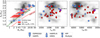 |
Fig. 1 THIRSTEE sample distributed in radius vs mass (left), equilibrium temperature (middle), and stellar effective temperature (right). Blue markers represent planets with an existing mass measurement in the literature and red markers represent those without one. TOI-406 b is shown in purple because this work represents the planet’s first mass measurement. Marker symbols correspond to the instruments the THIRSTEE survey is using to measure the mass of each planet. Underlying contours show the relative population of confirmed planets with better than 25% measurement precision in mass, according to data from the NEA accessed on August 27, 2024. Left: THIRSTEE targets without mass measurements are shown as bars, representing the range of their expected mass given their radius (e.g. Parviainen et al. 2024a). Curves representing an Earth-like and a pure iron composition are shown for reference (Zeng et al. 2019). Middle: equilibrium temperature taken from the literature where available. If unavailable, it was calculated assuming perfect day-night heat redistribution and zero Bond albedo. Right: for unconfirmed planet candidates, stellar effective temperature taken from the TICv8. |
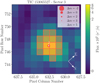 |
Fig. 2 tpfplotter TPF image of TOI-406 as in sector 3. The TESS aperture used to extract the photometry is shown with red squares. Gaia DR3 (Gaia Collaboration 2023) stars are represented as red circles, with sizes proportional to their magnitude. TOI-406 is positioned at the centre (star 1). Star 2 is a G = 16.887 mag star whose contribution to the aperture flux was accounted for by the SPOC pipeline through the calculation of the crowding metric and subtraction of the corresponding percentage (<O.14 percent in all four sectors) of the median flux level to account for dilution. The TPFs of all sectors are shown in Appendix A. |
4 Ground-based follow-up observations
Hord et al. (2024) already statistically validated the planetary nature of TOI-406 b using several ground-based followup observations. Here, we detail the additional photometric and RV observations that we used to measure the masses and densities of the planets in the system.
4.1 LCOGT photometry
TESS has a pixel scale of ~21″ pixel−1. This can cause multiple stars to be blended in the TESS aperture, since photometric apertures generally extend out to about 1 arcminute. In the attempt to identify the real source of the TESS transit detection, we performed ground-based follow-up photometry of the field around TOI-406 as part of the TFOP, scheduling the transit observations with the TESS Transit Finder tool (Jensen 2013).
We observed three transit windows of TOI-406 b on UTC October 30, 2020, August 29, 2021, and November 3, 2021, in Johnson/Cousins I band and Sloan 𝑔′ (November 3, 2021) from the Las Cumbres Observatory Global Telescope (LCOGT) (Brown et al. 2013) 1-m network node at Cerro Tololo Inter-American Observatory (CTIO) in Chile. We observed a partial and a full transit window on UT February 5, 2019, and October 24, 2022, respectively, in the Sloan i′ band from the LCOGT 1 m network node at South Africa Astronomical Observatory (SAAO) near Sutherland, South Africa. We also observed another full transit window on UT October 15, 2023, in the Sloan i′ band from the LCOGT lm network node at Siding Spring Observatory (SSO) near Coonabarabran, Australia. We calibrated the images using the standard LCOGT BANZAI pipeline (McCully et al. 2018), and we extracted differential photometry with AstroImageJ (Collins et al. 2017) using an aperture radius of 3″.1 that excluded all of the flux from the nearest known neighbour in the Gaia DR3 catalogue (Gaia DR3 4851053994762099840) that is 4″.2 south of TOI-406. A ~2.5 ppt event was detected on target in all observations. We included all the resulting light curves9 in our global modelling (Sect. 6.3).
The ground-based observations of TOI-406.02 taken with LCOGT were used to rule out unrecognised eclipsing binaries located inside TESS photometric aperture that could mimic a planetary signal. However, given the shallow transit depth (~0.8 ppt) of TOI-406.02, the transit detection for the existing ground-based LCOGT light curves (not shown) were highly dependent on the detrending parameters and photometric aperture used in the analysis, leading to some ambiguity in the transit evidence. Therefore, we did not include these light curves in the global fit.
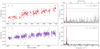 |
Fig. 3 ASAS-SN photometry of TOI-406 in V and g filters. Right panel: GLS periodogram of ASAS-SN photometry. The horizontal dashed and dotted lines represent the FAP level of 1% and 10%, respectively. The vertical red line shows the most significant peak. |
4.2 Long-term photometric monitoring
TOI-406 was observed by the All-Sky Automated Survey for Supernovae (ASAS-SN; Shappee et al. 2014, Kochanek et al. 2017) between 2014 and 2024. We retrieved the archival long-term photometry from the ASAS-SN portal10 (Hart et al. 2023), finding time series both in the V (~370 epochs) and 𝑔 (~1200 epochs) filters, spanning ~1570 days and ~2380 days, respectively (Fig. 3). Before proceeding with the analysis, we selected only the observations flagged as good quality (QUALITY=G), and we performed outlier rejection by doing a 5σ clipping, following (Hart et al. 2023). For the V filter, the photometry resulted in a median value of V = 13.92 mag, with a median uncertainty of σV = 0.006 mag and a root mean square (RMS) of 0.04 mag, while for the g filter we obtained 𝑔 = 14.57 mag, with a median uncertainty of σ𝑔 = 0.009 mag and an RMS of 0.06 mag. The ASAS-SN photometry, even if not appropriate to detect the transit events due to the relatively high uncertainty and cadence (generally > 2 d), has been used to investigate the stellar activity and the rotation period of the star (see Sect. 5.2).
4.3 ESPRESSO spectroscopic observations
As part of the THIRSTEE project, we collected 44 spectra within the lll.24PJ.001 program (PI: E. Pallé) using the Echelle Spectrograph for Rocky Exoplanets and Stable Spectroscopic Observations (ESPRESSO) installed at the Very Large Telescope (VLT) telescope array in the ESO Paranal Observatory, Chile (Pepe et al. 2021), with the goal of precisely determining the masses of the candidate planets and searching for additional planetary signals. The observations started on July 14, 2023, and ended on September 25, 2023. All measurements were gathered using ESPRESSO’S single Unit Telescope (lUT) in high-resolution (HR) mode (1 arcsec fibre, R ~ 140000) over a spectral range from ~380 to ~780 nm, with 2 × 1 detector binning (HR21). Observations were carried out with fibre B placed on the sky, to measure and subtract the background and possible moon contamination. The exposure time was set to 1200 seconds, which resulted in a median signal-to-noise ratio (S/N) of 23 at 550 nm. We reduced the data using the ESPRESSO data reduction pipeline (DRS), version 3.0.0. We extracted the RV values with the widely used template-matching algorithm SERVAL11 (Zechmeister et al. 2018). The resulting SERVAL-extracted RVs have an RMS of 4.3 m s−1 and a median individual uncertainty of 0.5 m s−1. The RV data and the associated activity indicators (see Sect. 5.2 for more details) are listed in Table C.1.
4.4 NIRPS/HARPS spectroscopic observations
TOI-406 was observed simultaneously from August 25, 2023, to March 16, 2024, with the Near-InfraRed Planet Searcher (NIRPS; Bouchy et al. 2017; Wildi et al. 2022) and the High Accuracy Radial velocity Planet Searcher (HARPS; Pepe et al. 2002), both of which are installed on the ESO 3.6-m telescope at La Silla, Chile. Both instruments are fibre-fed, stabilised, high-resolution echelle spectrographs, with NIRPS operating in the near-infrared (980–1800 nm) under an adaptive optics system, and HARPS working in the optical domain (330–690nm) in seeing-limited conditions. The observations were conducted as part of the NIRPS-GTO (Artigau et al. 2024) Follow-up of Transiting Planets sub-program (PID: 111.254T.001, 112.25NS.001; PI: Bouchy & Doyon) in high-efficiency modes; that is, the HE mode for NIRPS (R ≈ 70000, 0.9″ fibre) and the EGGS mode for HARPS (R ≈ 80000, 1.4″ fibre). Over 55 individual nights, we collected two spectra of TOI-406 per night with NIRPS (900 sec per exposure), plus a single spectra for an additional night, yielding a median SNR of 71.1 per pixel in the middle of H band. As NIRPS operated alone for nine nights, the HARPS dataset comprise 47 spectra (a single 1800 sec exposure per night) with a median SNR of 10.7 per pixel near 550 nm. The NIRPS data were reduced with the APERO pipeline (v0.7.290; Cook et al. 2022), the standard DRS for the SPIRou spectrograph (Donati et al. 2020), which is also compatible with NIRPS. APERO is optimised for near-infrared spectroscopy with many routines specifically developed and refined over the years to address challenges associated with this spectral domain such as telluric contamination, hot pixels, and detector persistence. For HARPS, we used the extracted spectra from the HARPS DRS (Lovis & Pepe 2007) available through the DACE platform12. The RVs were measured from the processed data using the line-by-line algorithm described in Artigau et al. (2022), which is publicly available (v0.69; LBL13). The LBL package is compatible with both NIRPS and HARPS. The method is conceptually similar to template matching (e.g. Anglada-Escudé & Butler 2012, Astudillo-Defru et al. 2017), while being more resilient to outlying spectral features (e.g. telluric residuals, cosmic rays, detector defects) as the template fitting is performed line by line, which facilitates the identification and removal of outliers. For NIRPS, we used the template of a brighter star with a similar spectral type, GJ 643 (M3.5V), from NIRPS-GTO observations. For HARPS, we instead employed the template of GL 699 (M4V) from public data obtained via the ESO archive (Delmotte et al. 2006). An additional telluric correction was performed for HARPS inside the LBL code by fitting a TAPAS atmospheric model (Bertaux et al. 2014).
We removed four outlying epochs (eight measurements) for NIRPS with velocities about 30 m/s above average. These epochs at barycentric earth radial velocity (BERV) of 12.2–13.1 km/s could be biased by telluric residuals (imperfect correction) that align with the stellar lines within a line width (that is, with a full width at half maximum (FWHM) of ~ 5 km/s) given that the systemic velocity of TOI-406 is 15.0 km/s. All other epochs were taken at BERV ranging from −16.6 and 9.5 km/s; that is, well outside of one line width of stellar velocity. We also discarded four HARPS measurements with imprecise velocities, each with a low SNR below 3. The final NIRPS (101) and HARPS (43) RVs have a median uncertainty of 4.40 m/s and 3.73 m/s and an RMS of 7.21 m/s and 7.43 m/s, respectively. The NIRPS and HARPS RV data and the associated activity indicators (see Sect. 5.2 for more details) are listed in Tables C.2 and C.3, respectively.
5 The star
5.1 Stellar parameters
We derived the stellar atmospheric parameters of TOI-406 using STEPARSYN14 (Tabernero et al. 2022) applied to the ESPRESSO spectra. We employed a grid of synthetic spectra generated using the Turbospectrum code (Plez 2012) in combination with the BT-Settl stellar atmospheric models (Allard et al. 2012), and atomic and molecular data from the Vienna atomic line database (VALD3, see Ryabchikova et al. 2015). We employed a list of Fe I and Ti I lines, along with various TiO molecular bands, which have been shown to be well suited for the analysis of M-type stars (see Marfil et al. 2021 for more detail). From our analysis, we obtained the following stellar parameters: Teff = 3364 ± 17 K, log g = 4.69 ± 0.04 dex, and [M/H] = −0.08 ± 0.08 dex. The first set of error bars refers only to the internal errors, and to estimate a more realistic uncertainty on Teff, we added a systematic component to the errors, following Tayar et al. (2022), obtaining Teff = 3364 ± 100 K.
The effective temperature [M/H], and abundance measurements of several elements were also determined from the NIRPS spectrum using the analysis framework of Jahandar et al. (2024). The first step in the analysis consists of fitting both Teff and [M/H] through χ2 minimisation of several spectral regions using ACES stellar models (Allard et al. 2012; Husser et al. 2013) with a fixed log 𝑔 of 5.0, convolved to match the NIRPS resolution. The analysis yields Teff = 3399 ± 49 K and [M/H] = 0.0 ± 0.05 dex, in good agreement with the parameters inferred from the ESPRESSO spectrum. The values reported in Table 2 are the weighted averages of both ESPRESSO and NIRPS measurements; that is, Teff = 3392 ± 44 K and [M/H] = −0.02 ± 0.04 dex. Finally, a series of fits was performed to a fixed Teff = 3400 K on individual spectral lines of known chemical species to derive their elemental abundances. The results are summarised in Table 3.
We determined the photometric spectral energy distribution (SED) of TOI-406 (Fig. 4) by combining all broad-band photometry available from public archives, including the American Association of Variable Star Observers Photometric All-Sky Survey (APASS, Henden & Munari 2014), the Sloan Digital Sky Survey (APASS, York et al. 2000), the Gaia DR3 archive (Gaia Collaboration 2016, 2023), 2MASS (Skrutskie et al. 2006), and the Wide-field Infrared Survey Explorer archive (WISE, Wright et al. 2010). Observed magnitudes were converted into fluxes by using the zero points given in the Virtual Observatory SED Analyzer tool (VOSA, Bayo et al. 2008), and observed fluxes were transformed into absolute fluxes by employing the Gaia DR3 trigonometric parallax. As is shown in Fig. 4, TOI-406’s SED is purely photospheric up to ~25 µm. The stellar bolometric luminosity (L⋆ = 0.0193 ± 0.0003 L⊙) was obtained by integrating the observed SED. The stellar radius  was then computed via the Stefan-Boltzmann law, which states
  , where σSB is the Stefan-Boltzmann constant. We measured the stellar mass
  by using the mass-radius relation of Schweitzer et al. (2019, their Eq. (6)). As a consistency check, we obtained the surface gravity, log 𝑔 = 4.82 ± 0.11 (cm s−2), using our derived stellar mass and radius, which is compatible at the 1 σ level with the spectro-scopic value (log 𝑔 = 4.69 ± 0.04) obtained from the spectral fitting analysis.
Finally, we used the Gaia DR3 positions, proper motions, parallax, and systemic RV to compute the galactic heliocentric space velocities of TOI-406 (U = 44.05 ± 0.31 km s−1, V = −44.44 ± 0.29 km s−1, W = -0.18 ± 0.29 km s−1 ), in the directions of the Galactic centre, Galactic rotation, and north Galactic pole, respectively. According to the probabilistic approach of Bensby et al. (2014), the galactic kinematic indicates that TOI-406 is a thin disc population star. All the adopted astro-metric and photometric stellar properties of TOI-406 are listed in Table 2.
Stellar properties of TOI-406.
TOI-406 stellar abundances measured with NIRPS.
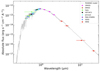 |
Fig. 4 SED for TOI-406. The grey line shows the BT-Settl model for Teff = 3300 K, log 𝑔 = 5.0 dex, and solar metallicity. |
5.2 Stellar activity indices and rotation period
We first analysed the periodicity of the TESS long-cadence SAP light curve15 and the long-term ASAS-SN photometry to identify the possible rotation period of the star. The generalised Lomb-Scargle (GLS, Zechmeister & Kürster 2009) periodogram of the TESS light curve identified a broad peak around 20-30 d, due to the different results of the 2018 (sectors 3, 4) and 2020 (sectors 30, 31) data, which, when analysed separately, show a significant peak at 28 and 21 days, respectively.
Both the ASAS-SN series show a periodicity around ~29 d, especially significant in the g filter (see Fig. 3). These results are further confirmed by the autocorrelation analysis we performed following the implementation of Angus (2021), from which we identify the main periodicity in the TESS and ASAS-SN g light curves at 28.7 and 28.5 days, respectively16.
We also investigated the stellar activity and assessed its impact on the RV measurements using a series of activity indicators (available on CDS). For the ESPRESSO dataset, we included in our analysis various absorption line indicators produced by the serval pipeline, such as the Na I doublet (λλ589.0 nm, 589.6 nm), the Hα (λ656.2 nm), and the S -index (Ca II H&K lines, λλ396.8470 nm, 393.3664 nm, computed with ACTIN217, Gomes da Silva et al. 2018; Gomes da Silva et al. 2021), as well as other SERVAL-derived activity indicators, such as the RV chromatic index (CRX) and the differential line width (dLW; see Zechmeister et al. 2018 and Jeffers et al. 2022 for a detailed description and discussion of the different indicators). In addition, we analysed the activity indexes automatically provided by the ESPRESSO DRS (Baranne et al. 1996; Pepe et al. 2002), such as the FWHM, the bisector span (BIS) (Queloz et al. 2001), and the contrast (Contr) of the cross-correlation function (CCF). For the CCF extraction, we used a M3 binary mask.
The GLS periodograms of the ESPRESSO RVs and the above-mentioned indexes are shown in Fig. 5. The periodogram of the RVs reveals the presence of a significant peak at ≃13 days (corresponding to one of the transiting candidates). This signal is also clearly identified in the GLS periodogram of the NIRPS RVs, and in the HARPS dataset, despite the lower significance (Fig. 6). Even though not particularly significant, we also identified in the ESPRESSO periodogram the presence of a signal at ~3.3 days, corresponding to the second planetary candidate (half of the period identified by TESS, see Sect. 6). Additionally, the ESPRESSO periodogram shows hints of a signal at ≃ 29 days, and a possible long-period signal peaking widely around 80–110 d. We note that such a signal is longer than the time-span of the ESPRESSO RV observations (~72 days), and therefore it cannot be accurately sampled using the current ESPRESSO dataset. The presence of these four significant peaks is further confirmed from our ℓ1 periodogram18 analysis (Fig. 7). The ℓ1 periodogram (Hara et al. 2017) is designed to search for periodicities in unevenly sampled time series, similarly to the GLS periodogram, but identifying fewer peaks due to aliasing. None of these additional signals are clearly identified in the NIRPS/HARPS datasets, (see Figs. 6 and 7), likely due to the higher scatter and internal errors with respect to the ESPRESSO dataset (Sect. 4).
Despite most of the ESPRESSO activity indexes not presenting significant periodic signals (false alarm probability, FAP < 10 %), the 29 d peak has a counterpart in the dLW, in the FWHM, and in the contrast of the CCF. This periodicity is also identified in the FWHM of the NIRPS dataset (Fig. 6)19.
The peak at ~29 d corresponds to the period signal identified in the TESS and ASAS-SN photometry. According to our activity analysis, we attributed this signal to the rotational period of the star. Moreover, using the log R′HK and the activity-rotation calibration for M dwarfs of Suárez Mascareño et al. (2016), we estimate a rotation period of  days, which is consistent within 1σ with the identified signal.
Even though not particularly active, as the low value of the log R′HK index indicates (log R′HK = −5.167 ± 0.017; derived from the median S -index using the calibrations of Suárez Mascareño et al. 2015 and adopting B – V = 1.464), from the activity analysis we concluded that the ESPRESSO RV data are affected by stellar activity variations. Therefore, to consistently model both the planetary and stellar signals, we selected the dLW20 series as a proxy of the stellar activity, and in our global analysis we fitted it simultaneously with the RVs (see Sect. 6) in a Gaussian processing (GP) regression framework, which also allowed us to determine the final adopted stellar rotation period ( days).
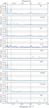 |
Fig. 5 GLS periodogram of the ESPRESSO RVs and the spectroscopic activity indicators. The vertical grey lines indicate the transit-like signals with periods of 13.176 and 3.307 days. The vertical red line shows the frequency corresponding to the possible rotational period of the star at ~29 days. The dashed, dash-dotted, and dotted horizontal lines show the 10%, 1%, and 0.1% FAP levels, respectively. |
 |
Fig. 7 ℓ1 periodogram of the ESPRESSO (left) and the combined NIRPS+HARPS datasets (right), computed on a grid of frequencies from 0 to 1 cycle per day. The total time span of the ESPRESSO and NIRPS/HARPS observations is ~72 and ~204 days, respectively. Each periodogram highlights in orange the significant peaks (with ∆ In 𝒵 > 10, where 𝒵 is the Bayesian evidence). |
6 Data analysis and results
6.1 Photometric fit
Given the ambiguity in the planetary period of the second TESS candidate (see Sect. 3), we first performed a photometric fit of the TESS light curve only to test the periodicity of TOI-406.02. We fitted a two-planet model using the retrieval code PyTransit21 (Parviainen 2015), including a GP regression with a Matérn-3/2 kernel to model the short-term periodicity. We parametrised the model of each planet using the planetary to stellar radius ratio (Rp/R⋆), mid-transit time (T0), period (P), impact parameter (b), a common stellar density (ρ⋆), two quadratic limb darkening (LD) coefficients, and an average white noise estimate. The LD coefficients were constrained using priors calculated with PyLDTk22 (Husser et al. 2013; Parviainen & Aigrain 2015). for TOI-406 b, we adopted uniform priors on T0 and P centred around the TESS TOI announcement values, with a central time window of +1 day and a period range of P ∈ [11,15] days. For TOI-406.02, we left the period free to vary between 1 and 8 days, and computed a T0 consistent with an orbital period of ~6.6 days and ~3.3 days, while using the same time window range of ±1 day. We adopted uniform, uninformative priors for the other parameters. The best-fitting period for TOI-406.02 from this analysis was 3.307 days, as is further confirmed by the RV analysis (Sect. 6.2) and by the joint modelling combining all photometric and RV information (Sect. 6.3). All other parameters from the transit fit are in agreement within 1σ with the values obtained from the joint modelling and adopted as final values in this work.
6.2 Radial velocity fit
To prove the feasibility of the THIRSTEE program and check if we can recover the planetary masses using only the THIRSTEE dataset, we performed a RV fit of the ESPRESSO-only data, and a joint fit including ESPRESSO and NIRPS/HARPS GTO data.
To model the RVs, we used PyORBIT23 (Malavolta et al. 2016, 2018), a Python package which allows for the modelling of planetary transits and RVs together with stellar activity effects. We assumed a two-planet Keplerian model, setting wide boundaries on the semi-amplitude, K (0.01–100 m s−1), for both candidates, and exploring the parameters in logarithmic space. We allowed the periods of the two planets to span between 2 and 20 days, while we assumed normal priors on T0 based on the values obtained from the photometric fit. We assumed the half-Gaussian zero-mean prior of Van Eylen et al. (2019) on the orbital eccentricity, e, and we adopted the parametrisation of Eastman et al. (2013), fitting  to determine the eccentricity and argument of periastron, ω. We modelled the stellar activity by including in the fit a GP regression with a quasi-periodic kernel (Grunblatt et al. 2015). We modelled simultaneously the RVs and the ESPRESSO dLW time series, which we selected as a proxy for the stellar activity given the presence of a significant periodic signal (Sect. 5.2), in order to better inform the GP (Langellier et al. 2021; Osborn et al. 2021; Barragán et al. 2023). We used two independent covariance matrices assuming common GP hyper-parameters (stellar rotation period Prot, characteristics decay timescale, Pdec, and coherence scale, w), except for the amplitude of the covariance matrix, which was fitted separately for the two time series. For each RV dataset, we included in the fit a systemic velocity term, and a jitter term to account for any underestimation of the error bars, possible systematics, and short-term stellar activity noise. Finally, given the hints of a possible long-period signal in the ESPRESSO RVs (Sect. 5.2), we included in the fit a second-order polynomial trend to take into account the long-term variability (with c0 as the x-intercept, c1 as the linear coefficient, and c2 as the quadratic coefficient).
We performed the RV fit with PyORBIT using the PyDE24 + emcee (Foreman-Mackey et al. 2013) set-up, as is detailed in Lacedelli et al. (2022, their Sect. 5), applying the same convergence criteria. We ran the chains with 2ndim walkers, where ndim is the dimensionality of the model, for 200 000 steps, discarding the first 30 000 steps as burn-in and using a thinning factor of 100.
In both cases (ESPRESSO-only and all available RV data), no signal was identified at 6.6 days, while the recovered periodicity for the TOI-406.02 candidate was 3.3 days, with an 8σ detection. This is in agreement with our photometric analysis (Sect. 6.1), and further confirms that the true period of the inner candidate (TOI-406 c hereafter) is half the proposed initial period. We list the retrieved semi-amplitude of the two planets from the ESPRESSO-only fit and from the fit including all the available RVs in Table 4, where only the values for TOI-406 b are discrepant but consistent within 1σ.
RV semi-amplitude of the TOI-406 planets.
6.3 Joint modelling of light curves and RVs
Finally, we performed the analysis of all the photometric and spectroscopic data using PyORBIT, adopting the model from the RV analysis (Sect. 6.2) and running the fit both in the ESPRESSO-only case and including all the RVs. We included in the model the TESS light curves, and the ground-based observation of TOI-406 b (see Sect. 4). Within PyORBIT, we modelled the light curves using the batman package (Kreidberg 2015), and fitting for each planet the T0, P, Rp/R⋆, b, a common ρ⋆, with a Gaussian prior based on our derived stellar parameters, and a jitter term for each dataset. We assumed a quadratic LD law on the coefficients, u1, u2, for each dataset, employing the LD parametrisation (q1, q2) introduced by Kipping (2013) and adopting a Gaussian prior with initial values obtained through PyLDTk25 (Husser et al. 2013; Parviainen & Aigrain 2015) with a custom large 1σ uncertainty of 0.1 for each coefficient. In the modelling of the TESS light curves, we incorporated a GP regression with a Matérn-3/2 kernel, to address potential correlated noise. To remove systematic instrumental effects, for each ground-based light curve we fitted together a quadratic term to detrend the data with respect to airmass. If not specified otherwise, we assumed uniform, uninformative priors for all the fitted parameters.
We performed the joint fit both using the ESPRESSO-only dataset, and using ESPRESSO+NIRPS+HARPS. As in the case of the RV fit only, the retrieved semi-amplitudes are virtually the same for TOI-406 c if using the ESPRESSO-only data or all available RVs, but slightly discrepant (but consistent within 1er) for TOI-406 b. We are unable to discriminate which solution is the most accurate and for completeness we adopted as final values the ones from the joint fit including all the available RVs. We list the results of our best-fitting model in Table 5, and we show the transit models, the phase-folded RVs, and the global RV model and in Figs. 8, 9, 10, and 11, respectively.
We confirm the planetary nature of the two candidates in the system, with orbital periods of Pc = 3.307 days (TOI-406 c) and Pb = 13.176 days (TOI-406 b). An important outcome of our RV frequency search in Sect. 5.2 was the absence of a signal at ~6.6 days; that is, the transiting candidate TOI-406.02 reported from the SPOC pipeline. However, we identified a signal with exactly half the period in the RV periodogram. Such a periodicity was also claimed as a possible alternative period for this candidate in the TESS EXOFOP web page. Our joint photometric and spectroscopic analysis confirms the detection of a planetary signal at 3.307 days, which we identify with TOI-406 c, and for which we inferred a precise mass ( , from the semi-amplitude Kc = 1.63 ± 0.12 m s−1) and radius (Rc = 1.32 ± 0.12 R⊕), implying an average density of pc = 4.9 ± 1.4 g cm−3.
The outer planet, TOI-406 b, has a radius of  , which, combined with the inferred mass of
  (from
(from  ), implies an average density of ρb = 4.1 ± 1.0 g cm−3. With our inferred parameters, planets b and c have equilibrium temperatures of Teq = 368 ± 14 K, and Teq = 584 ± 22 K, respectively.
From our analysis, we identify a possible long-term trend. However, such a long-term signal could be due both to a planetary companion or to stellar magnetic activity, and additional data of ESPRESSO-like precision covering a longer baseline are needed to understand its nature. This possible additional signal could also be the source of the slight discrepancy in the mass of TOI-406 b when using ESPRESSO-only data or all the available RVs.
The quasi-periodic GP modelling of the RVs and dLW results in the detection of a clear periodicity at Prot = 29.2 ± 0.5 days (see Fig. 11). This signal matches the period identified also in the ASAS-SN light curves and (marginally) in the TESS photometry (Sect. 5.2). We attribute this signal to the stellar rotational period, and we adopted the value inferred from our joint fit as its final value.
After the joint analysis, we could not identify any significant additional signals in the periodogram of the RV residuals in either the ESPRESSO-only case or in the case including all the RVs (Fig. 12). Moreover, we could not identify significant signals in the TESS light curve residuals by running a transit search using the transit least squares26 algorithm (Hippke & Heller 2019). We therefore conclude that with our current dataset we cannot identify additional planetary signals in the system.
Best-fit parameters of the TOI-406 system.
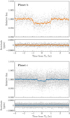 |
Fig. 8 Phase-folded TESS light curves of TOI-406 b and c. The best-fitting model is shown as a coloured line, and residuals are plotted in the bottom panels. The coloured dots indicate data points binned over 5 min. |
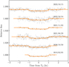 |
Fig. 9 Ground-based individual transit observations of TOI-406 b. Binned data points are shown with coloured dots, and the solid orange line indicates the best-fitting model. |
7 Discussion
7.1 TOI-406 planetary properties
One of the goals of the THIRSTEE project is to check whether planets around M dwarfs follow the mass-radius-density trends identified in Luque & Pallé (2022). Figure 13 shows the position of TOI-406 b and c in the mass-radius diagram of well-characterised small planets around M dwarfs (most recently updated by Parc et al. 2024). According to the theoretical tracks of Zeng et al. (2019), TOI-406 c is consistent with an Earthlike composition, even though its density is slightly lower than a pure rocky (Earth-like) planet, making it also consistent with the presence of a small amount of water mass fraction in the form of a supercritical steam atmosphere. In fact, rocky planets with a substantial water envelope and more irradiated than the runaway greenhouse limit can develop a supercritical steam atmosphere (Turbet et al. 2020), which implies a larger planetary radius, and therefore a slightly lower bulk density. The lower density of TOI-406 c with respect to a pure rocky composition could also hint at the presence of a secondary atmosphere, like for example that of 55 Cnc e (Ehrenreich et al. 2012; Tsiaras et al. 2016; Keles et al. 2022; Hu et al. 2024), TOI-561 b (Lacedelli et al. 2022; Brinkman et al. 2023; Patel et al. 2023), and similar planets that make up a significant fraction of the population of rocky planets currently being observed by JWST. On the other hand, TOI-406 b lies in a mass-radius region of high degeneracy in terms of interior composition (Fig. 13). The planet could host a significant amount of water, with a water mass fraction of up to 30% according to Aguichine et al. (2021) models of irradiated ocean planets, but it could also be consistent with a gas dwarf scenario; that is, a dry Earth-like core surrounded by a substantial H/He envelope, as is inferred from atmospheric mass loss theories (Owen & Wu 2013; Lopez & Fortney 2013; Gupta & Schlichting 2019; Wu 2019; Rogers et al. 2023).
These results are in line with the trend identified by Luque & Pallé (2022) for small planets around M dwarfs, where planets in the 1.4–2 R⊕ radius regime tend to fall into two distinct density regions, implying a different internal composition.
This outcome is also consistent with recent synthetic planet population simulations. In the core accretion scenario, planets generally develop into two distinct populations, one composed of a pure rocky core, and the other an ice-rock mixture containing ~50% ice. This ice fraction is characteristic of planetary components located beyond the water ice line (Thiabaud et al. 2014; Marboeuf et al. 2014). Icy and rocky pebbles have different physical properties, implying that icy cores are born bigger with respect to rocky ones, and this naturally explains the radius valley as an outcome of planet formation and evolution (Venturini et al. 2020, 2024; Burn et al. 2024), with most of the mini-Neptunes forming beyond the water ice line, and therefore being water-rich (Alibert et al. 2013; Raymond et al. 2018; Bitsch et al. 2018; Brügger et al. 2020; Izidoro et al. 2021; Venturini et al. 2020). Figure 14 shows the position of the two TOI-406 planets with respect to the synthetic population of M dwarfs planets presented in Venturini et al. (2024)27. The inner planet, TOI-406 c, is consistent with the population of planets having pure rocky cores, even though a small amount of volatiles could be present, suggesting a formation inside the ice line. On the other hand, the more external planet, TOI-406 b, is consistent with the population of planets having a substantial water mass fraction, suggesting a formation beyond the ice line and further inward migration after the disc dispersal. Moreover, recent studies show that more complex mechanisms, including the solubility of water in magma, magma ocean dynamics, envelope mixing, interactions between atmosphere and interiors, and redox reactions (i.e. Dorn & Lichtenberg 2021; Vazan et al. 2022; Lichtenberg & Miguel 2025; Luo et al. 2024; Rogers et al. 2024) could play an important role in the determination of the composition of small planets. However, independently of the model assumption and interpretation of the planetary composition, Fig. 15 shows that the TOI-406 planets fall into two distinct density populations, as is identified by Luque & Pallé (2022) and supporting the hypothesis of an observational density gap for small exoplan-ets orbiting M dwarfs. This hypothesis is further strengthened by the recent work of Schulze et al. (2024), which proves the statistical significance of such a density gap using mixture models in a hierarchical framework.
7.2 Dynamical analysis
We tested the dynamical stability of out best-fitting solution with the the REBOUND package Rein & Liu (2012); Rein & Spiegel (2015), computing the orbits of the system for 100 Kyr with the whfast integrator (with a fixed time-step of 0.1 d). We used the best-fitting parameters in Table 5) to draw ten initial sets of parameters based on a Gaussian distribution, and ran ten distinct simulations. During the integration, we used the mean exponential growth factor of nearby orbits (MEGNO or Y) indicator (Cincotta & Simó 2000; Rein & Tamayo 2016) to check the dynamical stability of the solution. We obtained a MEGNO value of 2 for all ten runs, proving the stability of this family of solutions.
To ascertain the dynamical stability of our best-fit solution, we also employed the reversibility error method (REM; Panichi et al. 2017), which has been demonstrated to be a close analogue of the maximum Lyapunov exponent. In the analysis of multi-body systems, it relies on numerical integration schemes that are time-reversible, in particular symplectic algorithms. This method is based on calculating the difference between the initial state vector and the final state vector, which is obtained by integrating the system of equations at a specific time and returning to the initial epoch. The difference thus defined will depend on the dynamic nature of the system.  or log
  means that the difference reaches the size of the orbit. The dynamical stability of the solution with REM was tested using the whf ast integrator with the 17th order corrector (with a fixed time step of 0.18 d) implemented within the REBOUND package for 100 000 orbital periods of the farthest planet. As is illustrated in Fig. 16, we obtained log
  , indicating that the solution is stable. Its position in the phase space demonstrates a non-resonant character. The visible resonant structure is at a safe distance, well above the uncertainty value of the orbital period of the outer planet. Like in the case of the MEGNO integrator, we also checked the stability for the family of solutions randomly selected from a Gaussian distribution based on our best-fitting parameters (Table 5). We ran 200 simulations for 100 Kyr, and we obtained log
  for all of them, confirming that the family of solutions is stable.
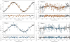 |
Fig. 10 Phase-folded RV fit with residuals from the joint photometric and RV analysis. The left column shows the fit using ESPRESSO data only, while the right one shows the results when including all the available RV data. The shaded area represents the ±1σ uncertainties of the model. The reported error bars include the jitter term added in quadrature, and the residuals are shown in the bottom panel. |
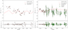 |
Fig. 11 Global RV model from the joint photometric and RV analysis. The left panel shows the fit using ESPRESSO data only, while the right one shows the results when including all the available RV data. Time is expressed in the TESS barycentric Julian date (TBJD). The grey line shows the best-fit global model, while the red line highlights the quasi-period GP regression component. The reported error bars include the jitter term added in quadrature, and the residuals are shown in the bottom panel. |
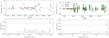 |
Fig. 12 Time series and GLS periodogram of the RV residuals after the joint photometric and spectroscopic fit (Sect. 6). The left panel shows the results using ESPRESSO data only, while the right one includes all the available RV data. In the bottom panel, the dashed and dotted horizontal lines show the 1 and 0.1 per cent FAP level, respectively. No significant peaks are present in either periodogram. |
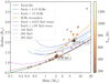 |
Fig. 13 Mass-radius diagram for small transiting planets around M dwarfs, colour-coded according to equilibrium temperature Teq. The TOI-406 planets are labelled, and highlighted with coloured diamonds. The sample was taken from the PlanetS catalogue (Parc et al. 2024) on July 30, 2024, reporting only planets with mass and radius determinations better than 25% and 8%, respectively. The solid green line indicates the theoretical composition models of Zeng et al. (2019) for an Earth-like composition (mass fractions of 32.5% iron and 67.5% silicates). The dotted dark blue lines correspond to Zeng et al. (2019) theoretical tracks of Earth-like rocky cores with H/He atmospheres by different percentages in mass at 300 K. The dotted orange line shows Rogers et al. (2023) mass-radius distribution derived from photoevaporation models. Dotted purple lines show Turbet et al. (2020) models for steam atmospheres, and the dash-dotted blue lines show Aguichine et al. (2021) compositional tracks at 400 K with a varying water mass fraction. |
7.3 Prospects for atmospheric characterisation
Given the possible presence of a gas layer in both planets and the need for additional constraints to break the degeneracy in planetary composition, we evaluated the feasibility of their atmospheric characterisation with JWST. To do so, we calculated the TSM and the emission spectroscopy metric (ESM) defined in Kempton et al. 2018).
Using the stellar and planetary parameters and Tables 2 and 5, TOI-406 c has TSM = 8.5 and ESM = 2.6, suggesting that its atmospheric characterisation would be a challenging task for JWST28. For TOI-406 b, which was the original target we included in our THIRSTEE sample, we obtained TSM = 43 and ESM = 1.0. Considering its radius and temperature, according to the classification of Hord et al. (2024), TOI-406 b lies in the top five best-in-class sample for JWST transmission spectroscopy follow-up, making it an interesting target with which to investigate the regime of small, low-temperature planets. In fact, with Teq = 368 ± 14 K, TOI-406 b adds up to the still-little population of cold planets (Teq < 400 K) with small radii (Rp <4 R⊕; Fig. 17). With an incident flux of only 3 ± 0.7 S⊕ (Pc = 13.17 d), the planet lies close to the inner edge of TOI-406’s empirical habitable zone (22 d < P < 92 d), as it is defined by Kaltenegger et al. (2019). As Fig. 17 shows, the planet has very similar properties to TOI-270 d (Rp~2.13 R⊕, Teq~350 K, TSM ~ 124; Günther et al. 2019), for which atmospheric features have recently been investigated and detected with HST and JWST (Mikal-Evans et al. 2023; Holmberg & Madhusudhan 2024; Benneke et al. 2024), demonstrating the potential of this category of planets for atmospheric characterisation, and placing TOI-406 b among the primary targets for future atmospheric follow-up.
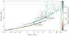 |
Fig. 14 Mass-radius diagram of synthetic planets with a period of less than 100 d at 2 Gyr around a 0.4 M⊙ star from the simulation of Venturini et al. (2024). Planets are colour-coded by water mass fraction. Most of the simulated planets belong to two distinct populations, of either purely rocky cores or planets containing about 50% water, plus a few of them have an extended envelope. The TOI-406 planets are labelled and highlighted with orange diamonds. TOI-406 c is consistent with the synthetic population of planets having rocky cores, while TOI-406 b seems to have a substantial water mass fraction. |
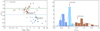 |
Fig. 15 Density properties of the well-characterised small-planet population around M dwarfs. Left: mass–density diagram for small transiting planets around M dwarfs, adapted from Luque & Pallé (2022). The TOI-406 planets are labelled, and highlighted with coloured diamonds. The sample is the same as in Fig. 13. Densities are normalised by Zeng et al. (2019) theoretical model of an Earth-like composition (scaled Earth bulk density, ρ⊕,s, assuming mass fractions of 32.5 % iron and 67.5% silicates). Planets are colour-coded according to their bulk densities, following Luque & Pallé (2022): Earth-like densities (brown), possible water worlds (cyan), and sub-Neptunes with H-He envelops (dark blue). The dotted blue line at 0.65 ρ⊕,s represents the compositional gap suggested by Luque & Pallé (2022). Right: normalised histogram of the sample of planets with mass and radius determinations better than 25% and 8%, respectively. Density is normalised to the Earth-like model. A Gaussian model fitted to the distribution of each planet population is shown with a solid coloured line. The red arrows show the positions of the TOI-406 planets in the density distributions. |
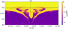 |
Fig. 16 Dynamical map for the solution presented in Table 5 for a wide range of orbital periods and eccentricities of the outer planet b. Small values of the fast indicator log |


8 Conclusions
In this paper, we present the THIRSTEE project, an observational survey that aims to shed light on the composition of the sub-Neptune population by increasing the number of accurately measured bulk density measurements across all stellar types and planet temperatures. We also aim to investigate their atmospheres to further probe their composition and perform statistical demographic studies of the sub-Neptune population.
We report the first results of the program, presenting the characterisation of a two-planet system orbiting the M dwarf TOI-406. Thanks to ESPRESSO and NIRPS/HARPS RV measurements, we could unveil the orbital architecture of the system, solving the ambiguity surrounding the orbital period of the inner candidate identified by TESS. According to our analysis, TOI-406 hosts a 3.3 d planet (Rc = 1.32 ± 0.12 R⊕,  , ρc = 4.9 ± 1.4 g cm−3) consistent with an Earthlike composition, and a temperate (Teq = 368 K) 13.2 d planet (
 ,
,  , ρb = 4.1 ± 1.1 g cm−3) compatible with multiple internal composition models, including a water-rich planet scenario. The bulk density of the two planets suggests that they fall into two distinct density populations, supporting the evidence for a density gap among the M dwarf population.
One of our important highlights is that TOI-406 b stands out as a particularly interesting target for atmospheric characterisation among low-temperature planets, where cloud formation processes are predicted to be less ubiquitous (Yu et al. 2021; Brande et al. 2024). The planet has very similar properties to TOI-270 d, for which atmospheric features have recently been detected with JWST, suggesting that it has high potential for atmospheric follow-up. Atmospheric characterisation will be essential to investigate the presence of the volatile component, break the degeneracy on the inner structure (Rogers & Seager 2010; Valencia et al. 2013; Fortney et al. 2013; Hu et al. 2021; Tsai et al. 2021; Schlichting & Young 2022), and probe cloud formation processes in sub-Neptunes. Finally, our data suggest the possible presence of a third external planet in addition to TOI-406 b and c, but additional data of ESPRESSO-qualit spanning a longer baseline are needed to investigate the nature (or existence) of this signal.
The TOI-406 planetary system shows the potential of the THIRSTEE program, laying a first stone on the path towards creating a reliable and wide observational sample of well-characterised sub-Neptunes. Such an observational sample is indeed needed for the comparison with planetary formation and evolution theories, as well as internal composition and atmospheric structure models, with the aim of improving our global picture of the sub-Neptune population.
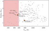 |
Fig. 17 Temperature-radius diagram for small well-characterised exo-planets. The sample was taken from the Planets catalogue (Parc et al. 2024), selecting only planets with Rp < 4 R⊕. TOI-406 b and c are labelled and highlighted with orange diamonds. The low-temperature region (Teq < 400 K) is highlighted in red. For comparison, planets with properties similar to TOI-406 b are labelled. |
Data availability
Full Tables C.1, C.2 and C.3 are available in electronic form at the CDS via anonymous ftp to cdsarc.cds.unistra.fr (130.79.128.5) or via https://cdsarc.cds.unistra.fr/viz-bin/cat/J/A+A/692/A238
Acknowledgements
We thank the anonymous referee for the comments that helped improving the quality of this paper. We acknowledge financial support from the Agencia Estatal de Investigación of the Ministerio de Ciencia e Innovación MCIN/AEI/10.13039/501100011033 and the ERDF “A way of making Europe” through project PID2021-125627OB-C32, and from the Centre of Excellence “Severo Ochoa” award to the Instituto de Astrofisica de Canarias. This paper includes data collected by the TESS mission, which are publicly available from the Mikulski Archive for Space Telescopes (MAST). Funding for the TESS mission is provided by the NASA Explorer Program. Resources supporting this work were provided by the NASA High-End Computing (HEC) Program through the NASA Advanced Supercomputing (NAS) Division at Ames Research Center for the production of the SPOC data products. This research has made use of the Exoplanet Follow-up Observation Program (ExoFOP; DOI: 10.26134/ExoFOP5) website, which is operated by the California Institute of Technology, under contract with the National Aeronautics and Space Administration under the Exoplanet Exploration Program. Funding for the TESS mission is provided by NASA’s Science Mission Directorate. This research has made extensive use of the SIMBAD database, operated at CDS, Strasbourg, France, and NASA’s Astrophysics Data System. This research has made use of the NASA Exoplanet Archive, which is operated by the California Institute of Technology, under contract with the National Aeronautics and Space Administration under the Exoplanet Exploration Program. This work has made use of data from the European Space Agency (ESA) mission Gaia (https://www.cosmos.esa.int/gaia), processed by the Gaia Data Processing and Analysis Consortium (DPAC, https://www.cosmos.esa.int/web/gaia/dpac/consortium). Funding for the DPAC has been provided by national institutions, in particular the institutions participating in the Gaia Multilateral Agreement. This publication makes use of data products from the Two Micron All Sky Survey, which is a joint project of the University of Massachusetts and the Infrared Processing and Analysis Center/California Institute of Technology, funded by the National Aeronautics and Space Administration and the National Science Foundation. This work makes use of observations from the LCOGT network. Part of the LCOGT telescope time was granted by NOIRLab through the Mid-Scale Innovations Program (MSIP). MSIP is funded by NSF.
This work has been carried out within the framework of the NCCR PlanetS supported by the Swiss National Science Foundation under grant 51NF40_205606. R.L. is supported by NASA through the NASA Hubble Fellowship grant HST-HF2-51559.001-A awarded by the Space Telescope Science Institute, which is operated by the Association of Universities for Research in Astronomy, Inc., for NASA, under contract NAS5-26555. R.L. also acknowledges funding from University of La Laguna through the Margarita Salas Fellowship from the Spanish Ministry of Universities ref. UNI/551/2021-May 26, and under the EU Next Generation funds. KAC and CNW acknowledge support from the TESS mission via subaward s3449 from MIT. J.M.A.M. is supported by the National Science Foundation (NSF) Graduate Research Fellowship Program (GRFP) under Grant No. DGE-1842400. J.M.A.M. and N.M.B. acknowledge support from NASA’S Interdisciplinary Consortia for Astrobiology Research (NNH19ZDA001N-ICAR) under award number 19-ICAR19_2-0041. D.J. and G.N. gratefully acknowledges the Centre of Informatics Tricity Academic Supercomputer and networK (CI TASK, Gda′nsk, Poland) for computing resources (grant no. PT01016). G.N. thanks for the research funding from the Ministry of Science and Higher Education programme the ‘Excellence Initiative - Research University’ conducted at the Centre of Excellence in Astrophysics and Astrochemistry of the Nicolaus Copernicus University in Toru′n, Poland. NN acknowledges funding from Light Bridges for the Doctoral Thesis ‘Habitable Earth-like planets with ESPRESSO and NIRPS’, in cooperation with the Instituto de Astrofísica de Canarias, and the use of Indefeasible Computer Rights (ICR) being commissioned at the ASTRO POC project in the Island of Tenerife, Canary Islands (Spain). The ICR-ASTRONOMY used for his research was provided by Light Bridges in cooperation with Hewlett Packard Enterprise (HPE). JIGH acknowledges financial support from the Spanish Ministry of Science and Innovation (MICINN) project PID2020-117493GB-I00. Research activities of the Board of Observational and Instrumental Astronomy at the Federal University of Rio Grande do Norte are supported by continuous grants from the Brazilian funding agencies CNPq. This study was financed in part by the CAPES-Print program. B.L.C.M. acknowledge CNPq research fellowships grant No. 305804/2022-7.
Appendix A TESS target pixel files
We show in Fig. A.1 the TPF plots for TOI-406 for all observed sectors save sector 3, which is shown in Fig. 2.
Appendix B TESS light curves
We show in Fig. B.1 the original and detrended TESS light curves of TOI-406 with our best-fit model.
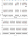 |
Fig. B.1 TESS sectors 3, 4 (top), and 30, 31 (bottom) PDCSAP light curves of TOI-406. In each figure, we show the best-fitting transit and Matérn-3/2 kernel GP model derived in Sect. 6 with a solid dark red line (top panel). The flattened light curve is shown in the central panel, after removing the GP component, with the solid red line showing the best-fitting model. The bottom panel shows the light curves residuals. The transits of planets b and c are highlighted with vertical orange and blue lines, respectively. |
Appendix C RV data
ESPRESSO RV measurements and activity indicators of TOI-406.
NIRPS RV measurements and activity indicators of TOI-406.
HARPS RV measurements and activity indicators of TOI-406.
References
- Adams, E. R., Jackson, B., Johnson, S., et al. 2021, Planet. Sci. J., 2, 152 [NASA ADS] [CrossRef] [Google Scholar]
- Aguichine, A., Mousis, O., Deleuil, M., & Marcq, E. 2021, ApJ, 914, 84 [NASA ADS] [CrossRef] [Google Scholar]
- Akana Murphy, J. M., Kosiarek, M. R., Batalha, N. M., et al. 2021, AJ, 162, 294 [NASA ADS] [CrossRef] [Google Scholar]
- Akana Murphy, J. M., Luque, R., & Batalha, N. M. 2024, arXiv e-prints [arXiv:2411.02521] [Google Scholar]
- Alibert, Y., Carron, F., Fortier, A., et al. 2013, A&A, 558, A109 [NASA ADS] [CrossRef] [EDP Sciences] [Google Scholar]
- Allard, F., Homeier, D., & Freytag, B. 2012, Philos. Trans. Roy. Soc. Lond. A, 370, 2765 [NASA ADS] [Google Scholar]
- Aller, A., Lillo-Box, J., Jones, D., Miranda, L. F., & Barceló Forteza, S. 2020, A&A, 635, A128 [NASA ADS] [CrossRef] [EDP Sciences] [Google Scholar]
- Anglada-Escudé, G., & Butler, R. P. 2012, ApJS, 200, 15 [Google Scholar]
- Angus, R. 2021, RuthAngus/starspot: code for measuring stellar rotation periods [Google Scholar]
- Artigau, É., Cadieux, C., Cook, N. J., et al. 2022, AJ, 164, 84 [NASA ADS] [CrossRef] [Google Scholar]
- Artigau, É., Bouchy, F., Doyon, R., et al. 2024, SPIE Conf. Ser., 13096, 130960C [Google Scholar]
- Astudillo-Defru, N., Díaz, R. F., Bonfils, X., et al. 2017, A&A, 605, L11 [EDP Sciences] [Google Scholar]
- Bailer-Jones, C. A. L., Rybizki, J., Fouesneau, M., Demleitner, M., & Andrae, R. 2021, VizieR Online Data Catalog, I/352 [Google Scholar]
- Baranne, A., Queloz, D., Mayor, M., et al. 1996, A&AS, 119, 373 [NASA ADS] [CrossRef] [EDP Sciences] [Google Scholar]
- Barragán, O., Gillen, E., Aigrain, S., et al. 2023, MNRAS, 522, 3458 [CrossRef] [Google Scholar]
- Batalha, N. M., Rowe, J. F., Bryson, S. T., et al. 2013, ApJS, 204, 24 [Google Scholar]
- Batalha, N. E., Lewis, T., Fortney, J. J., et al. 2019, ApJ, 885, L25 [Google Scholar]
- Bayo, A., Rodrigo, C., Barrado Y Navascués, D., et al. 2008, A&A, 492, 277 [NASA ADS] [CrossRef] [EDP Sciences] [Google Scholar]
- Bean, J. L., Raymond, S. N., & Owen, J. E. 2021, J. Geophys. Res. (Planets), 126, e06639 [NASA ADS] [Google Scholar]
- Benneke, B., Roy, P.-A., Coulombe, L.-P., et al. 2024, arXiv e-prints [arXiv:2403.03325] [Google Scholar]
- Bensby, T., Feltzing, S., & Oey, M. S. 2014, A&A, 562, A71 [NASA ADS] [CrossRef] [EDP Sciences] [Google Scholar]
- Berger, T. A., Huber, D., Gaidos, E., van Saders, J. L., & Weiss, L. M. 2020, AJ, 160, 108 [NASA ADS] [CrossRef] [Google Scholar]
- Bertaux, J. L., Lallement, R., Ferron, S., Boonne, C., & Bodichon, R. 2014, A&A, 564, A46 [NASA ADS] [CrossRef] [EDP Sciences] [Google Scholar]
- Bitsch, B., Morbidelli, A., Johansen, A., et al. 2018, A&A, 612, A30 [NASA ADS] [CrossRef] [EDP Sciences] [Google Scholar]
- Bitsch, B., Raymond, S. N., & Izidoro, A. 2019, A&A, 624, A109 [NASA ADS] [CrossRef] [EDP Sciences] [Google Scholar]
- Bonomo, A. S., Dumusque, X., Massa, A., et al. 2023, A&A, 677, A33 [NASA ADS] [CrossRef] [EDP Sciences] [Google Scholar]
- Borucki, W. J., Koch, D., Basri, G., et al. 2010, Science, 327, 977 [Google Scholar]
- Bouchy, F., Doyon, R., Artigau, É., et al. 2017, The Messenger, 169, 21 [NASA ADS] [Google Scholar]
- Brande, J., Crossfield, I. J. M., Kreidberg, L., et al. 2024, ApJ, 961, L23 [NASA ADS] [CrossRef] [Google Scholar]
- Brinkman, C. L., Weiss, L. M., Dai, F., et al. 2023, AJ, 165, 88 [NASA ADS] [CrossRef] [Google Scholar]
- Brown, T. M., Baliber, N., Bianco, F. B., et al. 2013, PASP, 125, 1031 [Google Scholar]
- Brügger, N., Burn, R., Coleman, G. A. L., Alibert, Y., & Benz, W. 2020, A&A, 640, A21 [NASA ADS] [CrossRef] [EDP Sciences] [Google Scholar]
- Burn, R., Schlecker, M., Mordasini, C., et al. 2021, A&A, 656, A72 [NASA ADS] [CrossRef] [EDP Sciences] [Google Scholar]
- Burn, R., Mordasini, C., Mishra, L., et al. 2024, Nat. Astron., 8, 463 [Google Scholar]
- Burt, J. A., Hooton, M. J., Mamajek, E. E., et al. 2024, ApJ, 971, L12 [NASA ADS] [CrossRef] [Google Scholar]
- Cadieux, C., Doyon, R., Plotnykov, M., et al. 2022, AJ, 164, 96 [NASA ADS] [CrossRef] [Google Scholar]
- Cadieux, C., Doyon, R., MacDonald, R. J., et al. 2024a, ApJ, 970, L2 [NASA ADS] [CrossRef] [Google Scholar]
- Cadieux, C., Plotnykov, M., Doyon, R., et al. 2024b, ApJ, 960, L3 [NASA ADS] [CrossRef] [Google Scholar]
- Castro-González, A., Díez Alonso, E., Menéndez Blanco, J., et al. 2022, MNRAS, 509, 1075 [Google Scholar]
- Chakrabarty, A., & Mulders, G. D. 2024, ApJ, 966, 185 [Google Scholar]
- Chaplin, W. J., Sanchis-Ojeda, R., Campante, T. L., et al. 2013, ApJ, 766, 101 [NASA ADS] [CrossRef] [Google Scholar]
- Cherubim, C., Cloutier, R., Charbonneau, D., et al. 2023, AJ, 165, 167 [NASA ADS] [CrossRef] [Google Scholar]
- Chontos, A., Murphy, J. M. A., MacDougall, M. G., et al. 2022, AJ, 163, 297 [NASA ADS] [CrossRef] [Google Scholar]
- Cincotta, P. M., & Simó, C. 2000, A&AS, 147, 205 [NASA ADS] [CrossRef] [EDP Sciences] [Google Scholar]
- Cloutier, R., Rodriguez, J. E., Irwin, J., et al. 2020, AJ, 160, 22 [NASA ADS] [CrossRef] [Google Scholar]
- Collins, K. 2019, in American Astronomical Society Meeting Abstracts, 233, 140.05 [NASA ADS] [Google Scholar]
- Collins, K. A., Kielkopf, J. F., Stassun, K. G., & Hessman, F. V. 2017, AJ, 153, 77 [Google Scholar]
- Cook, N. J., Artigau, É., Doyon, R., et al. 2022, PASP, 134, 114509 [NASA ADS] [CrossRef] [Google Scholar]
- Cutri, R. M., Skrutskie, M. F., van Dyk, S., et al. 2003, VizieR Online Data Catalog, 2246 [Google Scholar]
- Cutri, R., Wright, E. L., Conrow, T., et al. 2021, AllWISE Data Release [Google Scholar]
- Dai, F., Masuda, K., Winn, J. N., & Zeng, L. 2019, ApJ, 883, 79 [NASA ADS] [CrossRef] [Google Scholar]
- Delmotte, N., Dolensky, M., Padovani, P., et al. 2006, in Astronomical Society of the Pacific Conference Series, 351, Astronomical Data Analysis Software and Systems XV, eds. C. Gabriel, C. Arviset, D. Ponz, & S. Enrique, 690 [NASA ADS] [Google Scholar]
- Diamond-Lowe, H., Kreidberg, L., Harman, C. E., et al. 2022, AJ, 164, 172 [NASA ADS] [CrossRef] [Google Scholar]
- Díez Alonso, E., Suárez Gómez, S. L., González Hernández, J. I., et al. 2018, MNRAS, 476, L50 [CrossRef] [Google Scholar]
- Donati, J. F., Kouach, D., Moutou, C., et al. 2020, MNRAS, 498, 5684 [Google Scholar]
- Dorn, C., & Lichtenberg, T. 2021, ApJ, 922, L4 [NASA ADS] [CrossRef] [Google Scholar]
- Eastman, J., Gaudi, B. S., & Agol, E. 2013, PASP, 125, 83 [Google Scholar]
- Ehrenreich, D., Bourrier, V., Bonfils, X., et al. 2012, A&A, 547, A18 [NASA ADS] [CrossRef] [EDP Sciences] [Google Scholar]
- Esteves, L., Izidoro, A., Raymond, S. N., & Bitsch, B. 2020, MNRAS, 497, 2493 [Google Scholar]
- Fabrycky, D. C., Lissauer, J. J., Ragozzine, D., et al. 2014, ApJ, 790, 146 [Google Scholar]
- Foreman-Mackey, D., Hogg, D. W., Lang, D., & Goodman, J. 2013, PASP, 125, 306 [Google Scholar]
- Fortney, J. J., Mordasini, C., Nettelmann, N., et al. 2013, ApJ, 775, 80 [Google Scholar]
- Fulton, B. J., & Petigura, E. A. 2018, AJ, 156, 264 [Google Scholar]
- Fulton, B. J., Petigura, E. A., Howard, A. W., et al. 2017, AJ, 154, 109 [Google Scholar]
- Gaia Collaboration (Prusti, T., et al.) 2016, A&A, 595, A1 [NASA ADS] [CrossRef] [EDP Sciences] [Google Scholar]
- Gaia Collaboration (Vallenari, A., et al.) 2023, A&A, 674, A1 [NASA ADS] [CrossRef] [EDP Sciences] [Google Scholar]
- Ginzburg, S., Schlichting, H. E., & Sari, R. 2018, MNRAS, 476, 759 [Google Scholar]
- Gomes da Silva, J., Figueira, P., Santos, N., & Faria, J. 2018, J. Open Source Softw., 3, 667 [Google Scholar]
- Gomes da Silva, J., Santos, N. C., Adibekyan, V., et al. 2021, A&A, 646, A77 [NASA ADS] [CrossRef] [EDP Sciences] [Google Scholar]
- Grunblatt, S. K., Howard, A. W., & Haywood, R. D. 2015, ApJ, 808, 127 [NASA ADS] [CrossRef] [Google Scholar]
- Günther, M. N., Pozuelos, F. J., Dittmann, J. A., et al. 2019, Nat. Astron., 3, 1099 [Google Scholar]
- Gupta, A., & Schlichting, H. E. 2019, MNRAS, 487, 24 [Google Scholar]
- Hara, N. C., Boué, G., Laskar, J., & Correia, A. C. M. 2017, MNRAS, 464, 1220 [Google Scholar]
- Hart, K., Shappee, B. J., Hey, D., et al. 2023, arXiv e-prints [arXiv:2304.03791] [Google Scholar]
- Hawthorn, F., Bayliss, D., Wilson, T. G., et al. 2023, MNRAS, 520, 3649 [NASA ADS] [CrossRef] [Google Scholar]
- Henden, A., & Munari, U. 2014, Contrib. Astron. Observ. Skalnate Pleso, 43, 518 [NASA ADS] [Google Scholar]
- Hidalgo, D., Pallé, E., Alonso, R., et al. 2020, A&A, 636, A89 [NASA ADS] [CrossRef] [EDP Sciences] [Google Scholar]
- Hippke, M., & Heller, R. 2019, A&A, 623, A39 [NASA ADS] [CrossRef] [EDP Sciences] [Google Scholar]
- Hirano, T., Dai, F., Gandolfi, D., et al. 2018, AJ, 155, 127 [Google Scholar]
- Holmberg, M., & Madhusudhan, N. 2024, A&A, 683, L2 [NASA ADS] [CrossRef] [EDP Sciences] [Google Scholar]
- Hord, B. J., Kempton, E. M. R., Evans-Soma, T. M., et al. 2024, AJ, 167, 233 [NASA ADS] [CrossRef] [Google Scholar]
- Hu, R., Damiano, M., Scheucher, M., et al. 2021, ApJ, 921, L8 [NASA ADS] [CrossRef] [Google Scholar]
- Hu, R., Bello-Arufe, A., Zhang, M., et al. 2024, Nature, 630, 609 [NASA ADS] [CrossRef] [Google Scholar]
- Husser, T. O., Wende-von Berg, S., Dreizler, S., et al. 2013, A&A, 553, A6 [NASA ADS] [CrossRef] [EDP Sciences] [Google Scholar]
- Ikoma, M., & Hori, Y. 2012, ApJ, 753, 66 [NASA ADS] [CrossRef] [Google Scholar]
- Izidoro, A., Bitsch, B., Raymond, S. N., et al. 2021, A&A, 650, A152 [EDP Sciences] [Google Scholar]
- Izidoro, A., Schlichting, H. E., Isella, A., et al. 2022, ApJ, 939, L19 [NASA ADS] [CrossRef] [Google Scholar]
- Jahandar, F., Doyon, R., Artigau, É., et al. 2024, ApJ, 966, 56 [CrossRef] [Google Scholar]
- Jeffers, S. V., Barnes, J. R., Schöfer, P., et al. 2022, A&A, 663, A27 [NASA ADS] [CrossRef] [EDP Sciences] [Google Scholar]
- Jenkins, J. M. 2020, Kepler Data Processing Handbook, Kepler Science Document KSCI-19081-003 [Google Scholar]
- Jenkins, J. M., Twicken, J. D., McCauliff, S., et al. 2016, SPIE Conf. Ser., 9913, 1232 [Google Scholar]
- Jensen, E. 2013, Tapir: A web interface for transit/eclipse observability, Astrophysics Source Code Library [record ascl:1306.007] [Google Scholar]
- Kaltenegger, L., Pepper, J., Stassun, K., & Oelkers, R. 2019, ApJ, 874, L8 [NASA ADS] [CrossRef] [Google Scholar]
- Keles, E., Mallonn, M., Kitzmann, D., et al. 2022, MNRAS, 513, 1544 [NASA ADS] [CrossRef] [Google Scholar]
- Kempton, E. M. R., Bean, J. L., Louie, D. R., et al. 2018, PASP, 130, 114401 [Google Scholar]
- Kipping, D. M. 2013, MNRAS, 435, 2152 [Google Scholar]
- Kite, E. S., Fegley, Bruce, J., Schaefer, L., & Ford, E. B. 2019, ApJ, 887, L33 [NASA ADS] [CrossRef] [Google Scholar]
- Kochanek, C. S., Shappee, B. J., Stanek, K. Z., et al. 2017, PASP, 129, 104502 [Google Scholar]
- Korth, J., Csizmadia, S., Gandolfi, D., et al. 2019, MNRAS, 482, 1807 [Google Scholar]
- Kreidberg, L. 2015, PASP, 127, 1161 [Google Scholar]
- Lacedelli, G., Wilson, T. G., Malavolta, L., et al. 2022, MNRAS, 511, 4551 [NASA ADS] [CrossRef] [Google Scholar]
- Langellier, N., Milbourne, T. W., Phillips, D. F., et al. 2021, AJ, 161, 287 [NASA ADS] [CrossRef] [Google Scholar]
- Lee, E. J., & Chiang, E. 2016, ApJ, 817, 90 [Google Scholar]
- Lee, E. J., Chiang, E., & Ormel, C. W. 2014, ApJ, 797, 95 [Google Scholar]
- Lee, E. J., Karalis, A., & Thorngren, D. P. 2022, ApJ, 941, 186 [NASA ADS] [CrossRef] [Google Scholar]
- Léger, A., Selsis, F., Sotin, C., et al. 2004, Icarus, 169, 499 [Google Scholar]
- Lichtenberg, T., & Miguel, Y. 2025, Treatise Geochem., 7, 51 [Google Scholar]
- Lissauer, J. J., Ragozzine, D., Fabrycky, D. C., et al. 2011, ApJS, 197, 8 [Google Scholar]
- Liu, B., Ormel, C. W., & Lin, D. N. C. 2017, A&A, 601, A15 [NASA ADS] [CrossRef] [EDP Sciences] [Google Scholar]
- Livingston, J. H., Endl, M., Dai, F., et al. 2018, AJ, 156, 78 [Google Scholar]
- Lodders, K. 2003, ApJ, 591, 1220 [Google Scholar]
- Lopez, E. D., & Fortney, J. J. 2013, ApJ, 776, 2 [Google Scholar]
- Lovis, C., & Pepe, F. 2007, A&A, 468, 1115 [NASA ADS] [CrossRef] [EDP Sciences] [Google Scholar]
- Luo, H., Dorn, C., & Deng, J. 2024, Nat. Astron., 8, 1399 [Google Scholar]
- Luque, R., & Pallé, E. 2022, Science, 377, 1211 [NASA ADS] [CrossRef] [Google Scholar]
- Luque, R., Nowak, G., Pallé, E., et al. 2019, A&A, 623, A114 [NASA ADS] [CrossRef] [EDP Sciences] [Google Scholar]
- Luque, R., Serrano, L. M., Molaverdikhani, K., et al. 2021, A&A, 645, A41 [NASA ADS] [CrossRef] [EDP Sciences] [Google Scholar]
- Luque, R., Nowak, G., Hirano, T., et al. 2022, A&A, 666, A154 [NASA ADS] [CrossRef] [EDP Sciences] [Google Scholar]
- MacDougall, M. G., Petigura, E. A., Gilbert, G. J., et al. 2023, AJ, 166, 33 [NASA ADS] [CrossRef] [Google Scholar]
- Madhusudhan, N., Sarkar, S., Constantinou, S., et al. 2023, ApJ, 956, L13 [NASA ADS] [CrossRef] [Google Scholar]
- Malavolta, L., Nascimbeni, V., Piotto, G., et al. 2016, A&A, 588, A118 [NASA ADS] [CrossRef] [EDP Sciences] [Google Scholar]
- Malavolta, L., Mayo, A. W., Louden, T., et al. 2018, AJ, 155, 107 [NASA ADS] [CrossRef] [Google Scholar]
- Marboeuf, U., Thiabaud, A., Alibert, Y., Cabral, N., & Benz, W. 2014, A&A, 570, A36 [NASA ADS] [CrossRef] [EDP Sciences] [Google Scholar]
- Marcy, G. W., Isaacson, H., Howard, A. W., et al. 2014a, ApJS, 210, 20 [NASA ADS] [CrossRef] [Google Scholar]
- Marcy, G. W., Weiss, L. M., Petigura, E. A., et al. 2014b, PNAS, 111, 12655 [NASA ADS] [CrossRef] [Google Scholar]
- Marfil, E., Tabernero, H. M., Montes, D., et al. 2021, A&A, 656, A162 [NASA ADS] [CrossRef] [EDP Sciences] [Google Scholar]
- Mayor, M., Marmier, M., Lovis, C., et al. 2011, arXiv e-prints [arXiv: 1109.2497] [Google Scholar]
- McCully, C., Volgenau, N. H., Harbeck, D.-R., et al. 2018, SPIE Conf. Ser., 10707, 107070K [Google Scholar]
- Mikal-Evans, T., Madhusudhan, N., Dittmann, J., et al. 2023, AJ, 165, 84 [NASA ADS] [CrossRef] [Google Scholar]
- Mistry, P., Prasad, A., Maity, M., et al. 2024, PASA, 41, e030 [Google Scholar]
- Mousis, O., Deleuil, M., Aguichine, A., et al. 2020, ApJ, 896, L22 [NASA ADS] [CrossRef] [Google Scholar]
- Mulders, G. D., Pascucci, I., Apai, D., & Ciesla, F. J. 2018, AJ, 156, 24 [Google Scholar]
- Ogihara, M., Kunitomo, M., & Hori, Y. 2020, ApJ, 899, 91 [NASA ADS] [CrossRef] [Google Scholar]
- Osborn, A., Armstrong, D. J., Cale, B., et al. 2021, MNRAS, 507, 2782 [NASA ADS] [CrossRef] [Google Scholar]
- Osborne, H. L. M., Van Eylen, V., Goffo, E., et al. 2023, MNRAS, 527, 11138 [NASA ADS] [CrossRef] [Google Scholar]
- Otegi, J. F., Bouchy, F., & Helled, R. 2020, A&A, 634, A43 [NASA ADS] [CrossRef] [EDP Sciences] [Google Scholar]
- Owen, J. E., & Wu, Y. 2013, ApJ, 775, 105 [Google Scholar]
- Owen, J. E., & Wu, Y. 2016, ApJ, 817, 107 [NASA ADS] [CrossRef] [Google Scholar]
- Panichi, F., Gozdziewski, K., & Turchetti, G. 2017, MNRAS, 468, 469 [Google Scholar]
- Parc, L., Bouchy, F., Venturini, J., Dorn, C., & Helled, R. 2024, A&A, 688, A59 [NASA ADS] [CrossRef] [EDP Sciences] [Google Scholar]
- Parviainen, H. 2015, MNRAS, 450, 3233 [Google Scholar]
- Parviainen, H., & Aigrain, S. 2015, MNRAS, 453, 3821 [Google Scholar]
- Parviainen, H., Luque, R., & Palle, E. 2024a, MNRAS, 527, 5693 [Google Scholar]
- Patel, J. A., Egger, J. A., Wilson, T. G., et al. 2023, A&A, 679, A92 [NASA ADS] [CrossRef] [EDP Sciences] [Google Scholar]
- Pepe, F., Mayor, M., Galland, F., et al. 2002, A&A, 388, 632 [NASA ADS] [CrossRef] [EDP Sciences] [Google Scholar]
- Pepe, F., Mayor, M., Rupprecht, G., et al. 2002, The Messenger, 110, 9 [NASA ADS] [Google Scholar]
- Pepe, F., Cristiani, S., Rebolo, R., et al. 2021, A&A, 645, A96 [NASA ADS] [CrossRef] [EDP Sciences] [Google Scholar]
- Petigura, E. A., Howard, A. W., & Marcy, G. W. 2013, PNAS, 110, 19273 [NASA ADS] [CrossRef] [Google Scholar]
- Petigura, E. A., Rogers, J. G., Isaacson, H., et al. 2022, AJ, 163, 179 [NASA ADS] [CrossRef] [Google Scholar]
- Piaulet, C., Benneke, B., Almenara, J. M., et al. 2023, Nat. Astron., 7, 206 [Google Scholar]
- Piaulet-Ghorayeb, C., Benneke, B., Radica, M., et al. 2024, ApJ, 974, L10 [NASA ADS] [CrossRef] [Google Scholar]
- Plez, B. 2012, Turbospectrum: Code for spectral synthesis, Astrophysics Source Code Library [record ascl:1205.004] [Google Scholar]
- Polanski, A. S., Lubin, J., Beard, C., et al. 2024, ApJS, 272, 32 [NASA ADS] [CrossRef] [Google Scholar]
- Queloz, D., Henry, G. W., Sivan, J. P., et al. 2001, A&A, 379, 279 [NASA ADS] [CrossRef] [EDP Sciences] [Google Scholar]
- Rajpaul, V. M., Buchhave, L. A., Lacedelli, G., et al. 2021, MNRAS, 507, 1847 [NASA ADS] [CrossRef] [Google Scholar]
- Raymond, S. N., Boulet, T., Izidoro, A., Esteves, L., & Bitsch, B. 2018, MNRAS, 479, L81 [Google Scholar]
- Rein, H., & Liu, S. F. 2012, A&A, 537, A128 [NASA ADS] [CrossRef] [EDP Sciences] [Google Scholar]
- Rein, H., & Spiegel, D. S. 2015, MNRAS, 446, 1424 [Google Scholar]
- Rein, H., & Tamayo, D. 2016, MNRAS, 459, 2275 [Google Scholar]
- Ricker, G. R., Winn, J. N., Vanderspek, R., et al. 2014, J. Astron. Telesc. Instrum. Syst., 1, 1 [Google Scholar]
- Rogers, J. G., Schlichting, H. E., & Owen, J. E. 2023, ApJ, 947, L19 [NASA ADS] [CrossRef] [Google Scholar]
- Rogers, L. A. 2015, ApJ, 801, 41 [Google Scholar]
- Rogers, L. A., & Seager, S. 2010, ApJ, 712, 974 [Google Scholar]
- Rogers, J. G., Schlichting, H. E., & Young, E. D. 2024, ApJ, 970, 47 [NASA ADS] [CrossRef] [Google Scholar]
- Rowe, J. F., Bryson, S. T., Marcy, G. W., et al. 2014, ApJ, 784, 45 [Google Scholar]
- Ryabchikova, T., Piskunov, N., Kurucz, R. L., et al. 2015, Phys. Scr, 90, 054005 [Google Scholar]
- Schlichting, H. E., & Young, E. D. 2022, Planet. Sci. J., 3, 127 [NASA ADS] [CrossRef] [Google Scholar]
- Schulze, J. G., Wang, J., Johnson, J. A., et al. 2024, Planet. Sci. J., 5, 71 [NASA ADS] [CrossRef] [Google Scholar]
- Schweitzer, A., Passegger, V. M., Cifuentes, C., et al. 2019, A&A, 625, A68 [NASA ADS] [CrossRef] [EDP Sciences] [Google Scholar]
- Shappee, B. J., Prieto, J. L., Grupe, D., et al. 2014, ApJ, 788, 48 [Google Scholar]
- Sinukoff, E., Howard, A. W., Petigura, E. A., et al. 2017, AJ, 153, 271 [CrossRef] [Google Scholar]
- Skrutskie, M. F., Cutri, R. M., Stiening, R., et al. 2006, AJ, 131, 1163 [NASA ADS] [CrossRef] [Google Scholar]
- Smith, J. C., Stumpe, M. C., Van Cleve, J. E., et al. 2012, PASP, 124, 1000 [Google Scholar]
- Stassun, K. G., Oelkers, R. J., Pepper, J., et al. 2018, AJ, 156, 102 [Google Scholar]
- Stumpe, M. C., Smith, J. C., Van Cleve, J. E., et al. 2012, PASP, 124, 985 [Google Scholar]
- Stumpe, M. C., Smith, J. C., Catanzarite, J. H., et al. 2014, PASP, 126, 100 [Google Scholar]
- Suárez Mascareño, A., Rebolo, R., González Hernández, J. I., & Esposito, M 2015, MNRAS, 452, 2745 [CrossRef] [Google Scholar]
- Suárez Mascareño, A., Rebolo, R., & González Hernández, J. I. 2016, A&A, 595 A12 [Google Scholar]
- Tabernero, H. M., Marfil, E., Montes, D., & González Hernández, J. I. 2022 A&A, 657, A66 [NASA ADS] [CrossRef] [EDP Sciences] [Google Scholar]
- Tayar, J., Claytor, Z. R., Huber, D., & van Saders, J. 2022, ApJ, 927, 31 [NASA ADS] [CrossRef] [Google Scholar]
- Teske, J., Wang, S. X., Wolfgang, A., et al. 2021, ApJS, 256, 33 [NASA ADS] [CrossRef] [Google Scholar]
- Thiabaud, A., Marboeuf, U., Alibert, Y., et al. 2014, A&A, 562, A27 [NASA ADS] [CrossRef] [EDP Sciences] [Google Scholar]
- Tinetti, G., Drossart, P., Eccleston, P., et al. 2018, Exp. Astron., 46, 135 [NASA ADS] [CrossRef] [Google Scholar]
- Tsai, S.-M., Innes, H., Lichtenberg, T., et al. 2021, ApJ, 922, L27 [NASA ADS] [CrossRef] [Google Scholar]
- Tsiaras, A., Rocchetto, M., Waldmann, I. P., et al. 2016, ApJ, 820, 99 [NASA ADS] [CrossRef] [Google Scholar]
- Turbet, M., Bolmont, E., Ehrenreich, D., et al. 2020, A&A, 638, A41 [NASA ADS] [CrossRef] [EDP Sciences] [Google Scholar]
- Valencia, D., Guillot, T., Parmentier, V., & Freedman, R. S. 2013, ApJ, 775, 10 [NASA ADS] [CrossRef] [Google Scholar]
- Van Eylen, V., Agentoft, C., Lundkvist, M. S., et al. 2018, MNRAS, 479, 4786 [Google Scholar]
- Van Eylen, V., Albrecht, S., Huang, X., et al. 2019, AJ, 157, 61 [Google Scholar]
- Vazan, A., Sari, R., & Kessel, R. 2022, ApJ, 926, 150 [NASA ADS] [CrossRef] [Google Scholar]
- Venturini, J., Guilera, O. M., Haldemann, J., Ronco, M. P., & Mordasini, C. 2020, A&A, 643, L1 [NASA ADS] [CrossRef] [EDP Sciences] [Google Scholar]
- Venturini, J., Ronco, M. P., Guilera, O. M., et al. 2024, A&A, 686, L9 [NASA ADS] [CrossRef] [EDP Sciences] [Google Scholar]
- Weiss, L. M., & Marcy, G. W. 2014, ApJ, 783, L6 [Google Scholar]
- Wildi, F., Bouchy, F., Doyon, R., et al. 2022, SPIE Conf. Ser., 12184, 121841H [NASA ADS] [Google Scholar]
- Wright, E. L., Eisenhardt, P. R. M., Mainzer, A. K., et al. 2010, AJ, 140, 1868 [Google Scholar]
- Wu, Y. 2019, ApJ, 874, 91 [NASA ADS] [CrossRef] [Google Scholar]
- Wyatt, M. C., Kral, Q., & Sinclair, C. A. 2020, MNRAS, 491, 782 [NASA ADS] [Google Scholar]
- Xie, J.-W. 2014, ApJS, 210, 25 [NASA ADS] [CrossRef] [Google Scholar]
- York, D. G., Adelman, J., Anderson, John E., J., et al. 2000, AJ, 120, 1579 [NASA ADS] [CrossRef] [Google Scholar]
- Yu, X., He, C., Zhang, X., et al. 2021, Nat. Astron., 5, 822 [NASA ADS] [CrossRef] [Google Scholar]
- Zechmeister, M., & Kürster, M. 2009, A&A, 496, 577 [CrossRef] [EDP Sciences] [Google Scholar]
- Zechmeister, M., Reiners, A., Amado, P. J., et al. 2018, A&A, 609, A12 [NASA ADS] [CrossRef] [EDP Sciences] [Google Scholar]
- Zeng, L., Jacobsen, S. B., Sasselov, D. D., et al. 2019, PNAS, 116, 9723 [Google Scholar]
- Zhang, J., Weiss, L. M., Huber, D., et al. 2021, AJ, 162, 89 [NASA ADS] [CrossRef] [Google Scholar]
For example, a 1.8 R⊕ planet (the most representative example of our sample) can have a mass between 2-10 M⊕ (Parviainen et al. 2024a).
We decided to analyse the SAP light curve instead of the PDCSAP for the search of the rotation period as this photometry is less affected by systematic pipeline correction that could over-correct/inject spurious signals (Smith et al. 2012; Stumpe et al. 2012, 2014).
According to the definition (Zechmeister et al. 2018), dLW samples the same effect as FWHM, that is, the changes in the absorption line widths of the spectrum related to the changes in the stellar flux caused by the active regions.
Data are available on https://zenodo.org/records/10719523
For planets with Rp < 1.5 R⊕, Kempton et al. (2018) proposes a threshold of TSM > 10 and ESM > 7.5.
All Tables
All Figures
|
Fig. 1 THIRSTEE sample distributed in radius vs mass (left), equilibrium temperature (middle), and stellar effective temperature (right). Blue markers represent planets with an existing mass measurement in the literature and red markers represent those without one. TOI-406 b is shown in purple because this work represents the planet’s first mass measurement. Marker symbols correspond to the instruments the THIRSTEE survey is using to measure the mass of each planet. Underlying contours show the relative population of confirmed planets with better than 25% measurement precision in mass, according to data from the NEA accessed on August 27, 2024. Left: THIRSTEE targets without mass measurements are shown as bars, representing the range of their expected mass given their radius (e.g. Parviainen et al. 2024a). Curves representing an Earth-like and a pure iron composition are shown for reference (Zeng et al. 2019). Middle: equilibrium temperature taken from the literature where available. If unavailable, it was calculated assuming perfect day-night heat redistribution and zero Bond albedo. Right: for unconfirmed planet candidates, stellar effective temperature taken from the TICv8. |
| In the text | |
|
Fig. 2 tpfplotter TPF image of TOI-406 as in sector 3. The TESS aperture used to extract the photometry is shown with red squares. Gaia DR3 (Gaia Collaboration 2023) stars are represented as red circles, with sizes proportional to their magnitude. TOI-406 is positioned at the centre (star 1). Star 2 is a G = 16.887 mag star whose contribution to the aperture flux was accounted for by the SPOC pipeline through the calculation of the crowding metric and subtraction of the corresponding percentage (<O.14 percent in all four sectors) of the median flux level to account for dilution. The TPFs of all sectors are shown in Appendix A. |
| In the text | |
|
Fig. 3 ASAS-SN photometry of TOI-406 in V and g filters. Right panel: GLS periodogram of ASAS-SN photometry. The horizontal dashed and dotted lines represent the FAP level of 1% and 10%, respectively. The vertical red line shows the most significant peak. |
| In the text | |
|
Fig. 4 SED for TOI-406. The grey line shows the BT-Settl model for Teff = 3300 K, log 𝑔 = 5.0 dex, and solar metallicity. |
| In the text | |
|
Fig. 5 GLS periodogram of the ESPRESSO RVs and the spectroscopic activity indicators. The vertical grey lines indicate the transit-like signals with periods of 13.176 and 3.307 days. The vertical red line shows the frequency corresponding to the possible rotational period of the star at ~29 days. The dashed, dash-dotted, and dotted horizontal lines show the 10%, 1%, and 0.1% FAP levels, respectively. |
| In the text | |
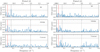 |
Fig. 6 Same as Figure 5, but for the NIRPS (left) and HARPS (right) datasets. |
| In the text | |
|
Fig. 7 ℓ1 periodogram of the ESPRESSO (left) and the combined NIRPS+HARPS datasets (right), computed on a grid of frequencies from 0 to 1 cycle per day. The total time span of the ESPRESSO and NIRPS/HARPS observations is ~72 and ~204 days, respectively. Each periodogram highlights in orange the significant peaks (with ∆ In 𝒵 > 10, where 𝒵 is the Bayesian evidence). |
| In the text | |
|
Fig. 8 Phase-folded TESS light curves of TOI-406 b and c. The best-fitting model is shown as a coloured line, and residuals are plotted in the bottom panels. The coloured dots indicate data points binned over 5 min. |
| In the text | |
|
Fig. 9 Ground-based individual transit observations of TOI-406 b. Binned data points are shown with coloured dots, and the solid orange line indicates the best-fitting model. |
| In the text | |
|
Fig. 10 Phase-folded RV fit with residuals from the joint photometric and RV analysis. The left column shows the fit using ESPRESSO data only, while the right one shows the results when including all the available RV data. The shaded area represents the ±1σ uncertainties of the model. The reported error bars include the jitter term added in quadrature, and the residuals are shown in the bottom panel. |
| In the text | |
|
Fig. 11 Global RV model from the joint photometric and RV analysis. The left panel shows the fit using ESPRESSO data only, while the right one shows the results when including all the available RV data. Time is expressed in the TESS barycentric Julian date (TBJD). The grey line shows the best-fit global model, while the red line highlights the quasi-period GP regression component. The reported error bars include the jitter term added in quadrature, and the residuals are shown in the bottom panel. |
| In the text | |
|
Fig. 12 Time series and GLS periodogram of the RV residuals after the joint photometric and spectroscopic fit (Sect. 6). The left panel shows the results using ESPRESSO data only, while the right one includes all the available RV data. In the bottom panel, the dashed and dotted horizontal lines show the 1 and 0.1 per cent FAP level, respectively. No significant peaks are present in either periodogram. |
| In the text | |
|
Fig. 13 Mass-radius diagram for small transiting planets around M dwarfs, colour-coded according to equilibrium temperature Teq. The TOI-406 planets are labelled, and highlighted with coloured diamonds. The sample was taken from the PlanetS catalogue (Parc et al. 2024) on July 30, 2024, reporting only planets with mass and radius determinations better than 25% and 8%, respectively. The solid green line indicates the theoretical composition models of Zeng et al. (2019) for an Earth-like composition (mass fractions of 32.5% iron and 67.5% silicates). The dotted dark blue lines correspond to Zeng et al. (2019) theoretical tracks of Earth-like rocky cores with H/He atmospheres by different percentages in mass at 300 K. The dotted orange line shows Rogers et al. (2023) mass-radius distribution derived from photoevaporation models. Dotted purple lines show Turbet et al. (2020) models for steam atmospheres, and the dash-dotted blue lines show Aguichine et al. (2021) compositional tracks at 400 K with a varying water mass fraction. |
| In the text | |
|
Fig. 14 Mass-radius diagram of synthetic planets with a period of less than 100 d at 2 Gyr around a 0.4 M⊙ star from the simulation of Venturini et al. (2024). Planets are colour-coded by water mass fraction. Most of the simulated planets belong to two distinct populations, of either purely rocky cores or planets containing about 50% water, plus a few of them have an extended envelope. The TOI-406 planets are labelled and highlighted with orange diamonds. TOI-406 c is consistent with the synthetic population of planets having rocky cores, while TOI-406 b seems to have a substantial water mass fraction. |
| In the text | |
|
Fig. 15 Density properties of the well-characterised small-planet population around M dwarfs. Left: mass–density diagram for small transiting planets around M dwarfs, adapted from Luque & Pallé (2022). The TOI-406 planets are labelled, and highlighted with coloured diamonds. The sample is the same as in Fig. 13. Densities are normalised by Zeng et al. (2019) theoretical model of an Earth-like composition (scaled Earth bulk density, ρ⊕,s, assuming mass fractions of 32.5 % iron and 67.5% silicates). Planets are colour-coded according to their bulk densities, following Luque & Pallé (2022): Earth-like densities (brown), possible water worlds (cyan), and sub-Neptunes with H-He envelops (dark blue). The dotted blue line at 0.65 ρ⊕,s represents the compositional gap suggested by Luque & Pallé (2022). Right: normalised histogram of the sample of planets with mass and radius determinations better than 25% and 8%, respectively. Density is normalised to the Earth-like model. A Gaussian model fitted to the distribution of each planet population is shown with a solid coloured line. The red arrows show the positions of the TOI-406 planets in the density distributions. |
| In the text | |
|
Fig. 16 Dynamical map for the solution presented in Table 5 for a wide range of orbital periods and eccentricities of the outer planet b. Small values of the fast indicator log |
| In the text | |
|
Fig. 17 Temperature-radius diagram for small well-characterised exo-planets. The sample was taken from the Planets catalogue (Parc et al. 2024), selecting only planets with Rp < 4 R⊕. TOI-406 b and c are labelled and highlighted with orange diamonds. The low-temperature region (Teq < 400 K) is highlighted in red. For comparison, planets with properties similar to TOI-406 b are labelled. |
| In the text | |
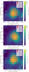 |
Fig. A.1 tpfplotter TPF image of TOI-406, as in Fig. 2, but for sectors 4, 30, 31. |
| In the text | |
|
Fig. B.1 TESS sectors 3, 4 (top), and 30, 31 (bottom) PDCSAP light curves of TOI-406. In each figure, we show the best-fitting transit and Matérn-3/2 kernel GP model derived in Sect. 6 with a solid dark red line (top panel). The flattened light curve is shown in the central panel, after removing the GP component, with the solid red line showing the best-fitting model. The bottom panel shows the light curves residuals. The transits of planets b and c are highlighted with vertical orange and blue lines, respectively. |
| In the text | |
Current usage metrics show cumulative count of Article Views (full-text article views including HTML views, PDF and ePub downloads, according to the available data) and Abstracts Views on Vision4Press platform.
Data correspond to usage on the plateform after 2015. The current usage metrics is available 48-96 hours after online publication and is updated daily on week days.
Initial download of the metrics may take a while.