| Issue |
A&A
Volume 688, August 2024
|
|
|---|---|---|
| Article Number | A216 | |
| Number of page(s) | 22 | |
| Section | Planets and planetary systems | |
| DOI | https://doi.org/10.1051/0004-6361/202450505 | |
| Published online | 27 August 2024 | |
Three super-Earths and a possible water world from TESS and ESPRESSO★
1
Observatoire de Genève, Département d’Astronomie, Université de Genève,
Chemin Pegasi 51b,
1290
Versoix,
Switzerland
e-mail: This email address is being protected from spambots. You need JavaScript enabled to view it.
2
Instituto de Astrofísica e Ciências do Espaço, CAUP, Universidade do Porto,
Rua das Estrelas,
4150-762
Porto,
Portugal
3
Departamento de Física e Astronomia, Faculdade de Ciências, Universidade do Porto,
Rua do Campo Alegre,
4169-007
Porto,
Portugal
4
Instituto de Astrofísica de Canarias,
c/ Vía Láctea s/n,
38205 La
Laguna,
Tenerife,
Spain
5
Physics Institute, University of Bern,
Gesellsschaftstrasse 6,
3012
Bern,
Switzerland
6
Center for Space and Habitability, University of Bern,
Gesellss-chaftstrasse 6,
3012
Bern,
Switzerland
7
Centro de Astrobiología (CAB), CSIC-INTA,
Camino Bajo del Castillo s/n,
28692,
Villanueva de la Cañada (Madrid),
Spain
8
INAF – Osservatorio Astronomico di Trieste,
via G. B. Tiepolo 11,
34143,
Trieste,
Italy
9
INAF – Osservatorio Astrofisico di Torino,
Strada Osservatorio 20,
10025,
Pino Torinese (TO),
Italy
10
European Southern Observatory,
Av. Alonso de Cordova,
3107,
Vitacura,
Santiago de Chile,
Chile
11
Jet Propulsion Laboratory, California Institute of Technology,
4800 Oak Grove Drive,
Pasadena,
CA
91109,
USA
12
Universidad de La Laguna, Dept. Astrofísica,
E-38206
La Laguna,
Tenerife,
Spain
13
Centro de Astrofísica da Universidade do Porto,
Rua das Estrelas,
4150-762
Porto,
Portugal
14
INAF – Osservatorio Astronomico di Palermo,
Piazza del Parla-mento 1,
90134
Palermo,
Italy
15
Instituto de Astrofísica e Ciências do Espaço, Faculdade de Ciências da Universidade de Lisboa,
1749-016
Lisboa,
Portugal
16
Observatoire François-Xavier Bagnoud – OFXB,
3961
Saint-Luc,
Switzerland
17
Departamento de Física de la Tierra y Astrofísica & IPARCOS-UCM (Instituto de Física de Partículas y del Cosmos de la UCM), Facultad de Ciencias Físicas, Universidad Complutense de Madrid,
28040
Madrid,
Spain
18
Centre for Exoplanets and Habitability, University of Warwick,
Coventry,
CV4 7AL,
UK
19
Department of Physics, University of Warwick,
Coventry
CV4 7AL,
UK
20
Caltech/IPAC-NASA Exoplanet Science Institute,
770 S. Wilson Avenue,
Pasadena,
CA
91106,
USA
21
Center for Astrophysics | Harvard & Smithsonian,
60 Garden Street,
Cambridge,
MA
02138,
USA
22
George Mason University,
4400 University Drive,
Fairfax,
VA
22030,
USA
23
NSF’s National Optical-Infrared Astronomy Research Laboratory,
950 N. Cherry Avenue,
Tucson,
AZ
85719,
USA
24
Dipartimento di Fisica, Università degli Studi di Torino,
Via Pietro Giuria, 1,
10125,
Torino,
Italy
25
NASA Ames Research Center,
Moffett Field,
CA
94035,
USA
26
Department of Physics and Astronomy, University of Louisville,
Louisville,
KY
40292,
USA
27
Astrobiology Center,
2-21-1 Osawa, Mitaka,
Tokyo
181-8588,
Japan
28
National Astronomical Observatory of Japan,
2-21-1 Osawa, Mitaka,
Tokyo
181-8588,
Japan
29
Department of Physics and Astronomy, University of New Mexico,
210 Yale Blvd NE,
Albuquerque,
NM
87106,
USA
30
Department of Physics and Kavli Institute for Astrophysics and Space Research, Massachusetts Institute of Technology,
Cambridge,
MA
02139,
USA
31
Department of Earth, Atmospheric and Planetary Sciences, Massachusetts Institute of Technology,
Cambridge,
MA
02139,
USA
32
Department of Aeronautics and Astronautics,
MIT, 77 Massachusetts Avenue,
Cambridge,
MA
02139,
USA
33
Perth Exoplanet Survey Telescope,
Perth,
Western Australia,
Australia
34
Department of Astrophysical Sciences, Princeton University,
Princeton,
NJ
08544,
USA
Received:
25
April
2024
Accepted:
10
June
2024
Abstract
Context. Since 2018, the ESPRESSO spectrograph at the VLT has been hunting for planets in the southern skies via the radial velocity (RV) method. One of its goals is to follow up on candidate planets from transit surveys such as the TESS mission, with a particular focus on small planets for which ESPRESSO’s RV precision is vital.
Aims. We aim to confirm and characterise, in detail, three super-Earth candidate transiting planets from TESS using precise RVs from ESPRESSO.
Methods. We analysed photometry from TESS and ground-based facilities, high-resolution imaging, and RVs from ESPRESSO, HARPS, and HIRES, to confirm and characterise three new planets: TOI-260 b, transiting a late K dwarf, and TOI-286 b and c, orbiting an early K dwarf. We also updated the parameters for the known super-Earth TOI-134 b (L 168-9 b), which is hosted by an M dwarf.
Results. TOI-260 b has a 13.475853−0.000011+0.000013 d period, 4.23 ± 1.60 M⊕ mass, and 1.71 ± 0.08 R⊕ radius. For TOI-286 b we find a 4.5117244−0.0000027+0.0000031 d period, 4.53 ± 0.78 M⊕ mass, and 1.42 ± 0.10 R⊕ radius; for TOI-286 c, we find a 39.361826−0.000081+0.000070 d period, 3.72 ± 2.22 M⊕ mass, and 1.88 ± 0.12 R⊕ radius. For TOI-134 b we obtain a 1.40152604−0.00000082+0.00000074 d period, 4.07 ± 0.45 M⊕ mass, and 1.63 ± 0.14 R⊕ radius. Circular models are preferred for all the planets, although for TOI-260 b the eccentricity is not well constrained. We computed bulk densities and placed the planets in the context of composition models.
Conclusions. TOI-260 b lies within the radius valley, and is most likely a rocky planet. However, the uncertainty on the eccentricity and thus on the mass renders its composition hard to determine. TOI-286 b and c span the radius valley, with TOI-286 b lying below it and having a likely rocky composition, while TOI-286 c is within the valley, close to the upper border, and probably has a significant water fraction. With our updated parameters for TOI-134 b, we obtain a lower density than previous findings, giving a rocky or Earth-like composition.
Key words: planets and satellites: individual: TOI-260 / planets and satellites: individual: TOI-286 / planets and satellites: individual: TOI-134
Tables B.1–B.4 are available at the CDS via anonymous ftp to cdsarc.cds.unistra.fr (138.79.128.5) or via https://cdsarc.cds.unistra.fr/viz-bin/cat/J/A+A/688/A216
© The Authors 2024
 Open Access article, published by EDP Sciences, under the terms of the Creative Commons Attribution License (https://creativecommons.org/licenses/by/4.0), which permits unrestricted use, distribution, and reproduction in any medium, provided the original work is properly cited.
This article is published in open access under the Subscribe to Open model. This email address is being protected from spambots. You need JavaScript enabled to view it. to support open access publication.
1 Introduction
Transiting planets orbiting around bright nearby stars are excellent targets for a detailed characterisation with follow-up high-resolution spectroscopy. By combining the transit photometry with the radial velocities (RVs) obtained from the spectra, both the radius and true mass can be determined. This in turn allows for the determination of the planet’s bulk density, which provides valuable constraints on its likely composition.
The Transiting Exoplanet Survey Satellite (TESS) NASA mission (Ricker et al. 2015) has been conducting an all-sky survey to search for transiting planet candidates around nearby stars since 2018, through its prime mission (25 July 2018–4 July 2020), first extended mission (4 July 2020-1 September 2022), and second extended mission (1 September 2022-present). One of the primary science requirements of the TESS prime mission was to determine the masses for at least 50 planets with radii <4 R⊕. This has been amply achieved, with 128 such planets with masses determined to date1, though only 97 have masses measured to an accuracy of 25% or better2. In order to achieve this requirement, TESS relies on extreme precision radial velocity (EPRV) facilities, which can confirm the TESS candidates and provide mass measurements.
The Echelle SPectrograph for Rocky Exoplanets and Stable Spectroscopic Observations (ESPRESSO, Pepe et al. 2013, 2021) is an EPRV spectrograph at ESO’s Very Large Telescope (VLT), Paranal, Chile. Achieving an RV precision of better than 25 cm s–1 during a single night, ESPRESSO is designed for and ideally suited to the precise mass measurement of low-mass planets. One of the main objectives of the ESPRESSO Guaranteed Time Observations (GTO, Pepe et al. 2021) is indeed the follow-up of such candidate planets from TESS and Kepler. The rocky planet population, especially, with masses typicup-dally below 6–8 M⊕, can only be characterised with instruments of ESPRESSO’s RV precision.
The population of planets with Rp < 4 R⊕ encompasses the super-Earth and sub-Neptune groups, types of planets that are not found in the Solar System but which are common in exo-planetary systems, with occurrence rates of ~30% (Fressin et al. 2013). The two groups are separated by a paucity of planets in the 1.5–2 R⊕ region, known as the radius valley or Fulton gap, which was predicted by Owen & Wu (2013) and confirmed by Fulton et al. (2017). The radius valley is thought to divide the smaller, rocky super-Earths from the larger, volatile-rich sub-Neptunes. The accurate characterisation of planets in this regime allows us to probe their likely composition, and also gain insights into their formation and evolution (e.g. Venturini et al. 2020a,b; Luque & Pallé 2022; Burn et al. 2024).
In this work, we present the confirmation and characterisation of three new planets in the super-Earth and sub-Neptune domains: TOI-260 b, TOI-286 b, and TOI-286 c. TOI-260 b, which has a 1.71 ± 0.11 R⊕ radius, orbits a late K dwarf with a ~13.5d period. TOI-286 b and TOI-286 c are hosted by an early K dwarf; the inner planet, TOI-286 b, has a 1.41 ± 0.07 R⊕ radius and a ~4.5 d period, while the outer planet, TOI-286 c, has a 1.86 ± 0.1 R⊕ radius and a ~39.4 d period. We also provide an update for the planetary parameters and characterisation of the previously confirmed planet TOI-134 b, also known as L 1689 b, which orbits an M dwarf at a ~1.4 d period. This planet was first described in Astudillo-Defru et al. (2020) and some of its parameters were updated by Patel & Espinoza (2022).
We describe the data in Sect. 2, and present our analysis of them in Sect. 3. Our results are discussed in Sect. 4, and we summarise and conclude in Sect. 5.
2 Observations
In this section we describe the data used to identify and confirm the new planets we present in this paper, TOI-260 b, TOI-286 b, and TOI-286 c. For TOI-134 b, which is a known planet, we present only the TESS data (some of which postdates the work of Astudillo-Defru et al. 2020 and Patel & Espinoza 2022) and the new ESPRESSO data which we used to refine the planetary mass.
2.1 TESS photometry
TOI-260 (TIC 37749396) has been observed by TESS three times: once in the prime mission (Cycle 1) in sector 3, using CCD 4 of camera 1; once in the first extended mission (Cycle 4) in sector 42, using CCD 4 of camera 2; and once in the second extended mission (Cycle 6) in sector 70, using CCD 1 of camera 1. All the observations were done in two-minute cadence.
TOI-286 (TIC 150030205) is in the TESS continuous viewing zone. It was observed by TESS in sectors 1-5 and 7-13 during the prime mission (Cycle 1); and 27-39 (Cycle 3) and 61-69 (Cycle 5) in the extended missions. It was observed in camera 4 throughout. CCD 1 was used for sectors 30-32; CCD 2 for sectors 3-5, 7-9, 33-36, and 61-63; CCD 3 for sectors 1012, 37-39, and 64-66; and CCD 4 for sectors 1-2, 27-29, and 67-69. All the observations were done in two-minute cadence.
TOI-134 (TIC 234994474) was observed by TESS in the prime mission in sector 1 (Cycle 1), and in the extended missions in sector 28 (Cycle 3) and sector 68 (Cycle 5). It was observed in camera 2, in CCD 2 for sector 1 and CCD 1 for sectors 28 and 68. All the observations were done in two-minute cadence.
All the TESS photometry was processed by the TESS Science Processing Operations Center (SPOC, Jenkins et al. 2016) at NASA Ames Research Center. Potential transit signals -corresponding to one planet candidate for TOI-260, two for TOI-286, and one for TOI-134 – were identified in the SPOC transit search (Jenkins 2002; Jenkins et al. 2010, 2020) of the light curve, and designated as TESS Objects of Interest (TOIs) by the TESS Science Office (Guerrero et al. 2021). The SPOC fit an initial limb-darkened transit model to each of these planetary signatures (Li et al. 2019) and subjected each to a suite of diagnostic tests (Twicken et al. 2018) to help make or break their planetary nature. In particular, the difference image cen-troiding analysis for the multi-sector searches3 constrained the location of the transit source for TOI-260, TOI-286 and TOI-134 to within 2.6 ± 6.7″, 2.8 ± 5.7″, and 3.6 ± 3.0″, respectively. For our analysis, we use the SPOC Presearch Data Conditioning Simple Aperture Photometry (PDC-SAP) light curves (Stumpe et al. 2012, 2014; Smith et al. 2012).
Due to its large pixel size of 21" per pixel, the TESS photometry can be contaminated by nearby companions. We used the tpfplotter package (Aller et al. 2020) to search for potential contaminants in the TESS apertures of our new planet hosts, TOI-260 and TOI-286. Since TOI-134 b is an already confirmed planet we do not apply this method to TOI-134. Figure 1 shows the resulting plots for sector 3 for TOI-260, and for sector 1 for TOI-286. The remaining sector plots are shown in online Appendix A4. For TOI-260, we do not identify any contaminants within the TESS aperture down to a magnitude contrast of 8, corresponding to the faintest blended binary that could mimic the transit depth (Lillo-Box et al. 2014). For TOI-286, there are three stars within the TESS aperture, most notably the close companion Gaia DR3 5482316884791610880, with a Gaia magnitude of 15.08 (corresponding to a Am = 5.42), and an angular separation of 16.7". This companion has a very different parallax and proper motion to TOI-286, and thus is likely not physically associated but is a chance alignment. We note that the SPOC difference image centroiding results strongly favour the target star as the source of the transit signal rather than the dimmer companion. Likewise, using a modified version of the TESS positional probability code of Hadjigeorghiou & Armstrong (2024), we find probabilities of 34% and 74% for the transits of the inner and outer candidates respectively to come from the target star, versus 24% probability for the transits of both candidates to come from the companion.
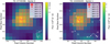 |
Fig. 1 TESS target pixel files for TOI-260 for sector 3 (left), and for TOI-286 for sector 1 (right). The remaining sectors are shown in online Appendix A. The target star is labelled as 1 and marked by a white cross in each case. All sources from the Gaίa DR3 catalogue down to a magnitude contrast of 8 are shown as red circles, with the size proportional to the contrast. The SPOC pipeline aperture is overplotted in shaded red squares. |
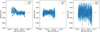 |
Fig. 2 Ground-based photometry for TOI-260, from LCO-CTIO (left), LCO-SSO (middle), and LCO-SAAO (right). The orange horizontal bars indicate the timespan of the closest transit to each observation; the vertical bars indicate the transit midpoint and depth. The timing of the observations was planned from preliminary ephemerides; later additional TESS data showed them to be out of transit. Note that the target star in these image sequences was intentionally either strongly exposed or saturated (causing large scatter and/or systematics) for the purpose of searching for an eclipsing binary in fainter neighbouring stars that could be the cause of the TESS detection. |
2.2 Ground-based photometry
Follow-up ground-based photometry is valuable to identify cases of false positives where the TESS photometry is contaminated by nearby companions, or conversely to rule out the possibility that the transit-like signal is caused by a close companion that is an eclipsing binary. This is particularly important for TOI-286, which has a close bright companion. TOI-286 and TOI-260 were each observed three times; we describe the observations below. We used the TESS Transit Finder, which is a customised version of the Tapir software package (Jensen 2013), to schedule our transit observations.
2.2.1 LCO
The Las Cumbres Observatory global telescope network (LCO, Brown et al. 2013) is a globally distributed network of telescopes. The 1 m telescopes used for TESS follow-up are equipped with 4096 × 4096 SINISTRO cameras which have an image scale of 0″.389 per pixel, resulting in a 26′ × 26′ field of view.
LCO observed TOI-260 three times from different sites: Once from the South African Astronomical Observatory (SAAO) site in Pan-STARRS Y-band (λc = 10040 Å, Width = 1120 Å), on 19 August 2019 ; once from the Siding Spring Observatory (SSO) site in Pan-STARRS z-short band (λc = 8700 Å, Width = 1040 Å), on 10 October 2020; and once from the Cerro Tololo Inter-American Observatory (CTIO) site in Pan-STARRS z-short band, on 7 July 2021. The images were calibrated by the standard LCOGT BANZAI pipeline (McCully et al. 2018), and photometric data were extracted using AstroImageJ (Collins et al. 2017). The target star light curves are shown in Fig. 2. Note that the target star in these and following image sequences was intentionally either strongly exposed or saturated (causing large scatter and/or systematics) for the purpose of searching for an eclipsing binary in fainter neighbouring stars that could be the cause of the TESS detection.
LCO also observed TOI-286 once, for a transit of the inner candidate TOI-286.01. The observation was done on 24 December 2018, in Sloan r′ filter, from the CTIO site. We highlight that the observation cleared the close companion Gaia DR3 5482316884791610880 of being a background eclipsing binary at this period. The target star light curve is shown in Fig. 3.
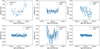 |
Fig. 3 Top: ground-based photometry for TOI-286, from LCO-CTIO (left), MKO (middle), and PEST (right). The orange (for planet 1) or green (for planet 2) horizontal bars indicate the timespan of the closest transit to each observation; the transit depth is too small to be seen. Note that the target star in these image sequences was intentionally either strongly exposed or saturated (causing large scatter and/or systematics) for the purpose of searching for an eclipsing binary in fainter neighbouring stars that could be the cause of the TESS detection. Bottom: ground based photometry for the close companion Gaia DR3 5482316884791610880, which clears it of being a background eclipsing binary. |
2.2.2 MKO
A full transit of TOI-286.01 was observed on 28 December 2018 in the Sloan r′ (530–700 nm) band from the 0.61 m University of Louisville Mt. Kent CDK700 (MKO CDK700), located at the University of Southern Queensland’s Mt. Kent Observatory near Toowoomba, Australia. The telescope had a 4096 × 4096 SBIG STX-16803 camera providing an image scale of 0″.74 per pixel, that resulted in a 27′ × 27′ field of view. The images were focused and seeing-limited to have typical stellar point-spread- functions with a full-width-half-maximum (FWHM) of 2″.3. The images were calibrated for bias and dark corrections with WCS coordinates used to locate the target and potential nearby-stars that would affect TESS photometry. Astrometry was obtained with Astrometry.net5 (Lang et al. 2010). Photometric data were extracted with AstroImageJ using a circular aperture with a 6.″70 radius. The resulting light curve was detrended against airmass. While a transit in the target was anticipated to be too shallow to detect from the ground, potential nearby eclipsing binary stars or other contributors were inspected and eliminated as possible sources of a TESS signal. The target star light curve is shown in Fig. 3.
2.2.3 PEST
The Perth Exoplanet Survey Telescope (PEST) is a backyard observatory near Perth, Australia, operated by Thiam-Guan Tan. The 0.3 m telescope is equipped with a 5544 × 3694 QHY183M camera. Images are binned 2×2 in software giving an image scale of 0.″77 pixel−1 resulting in a 32′ × 21′ field of view. PEST observed a transit of the outer candidate, TOI-286.02, on 6 November 2021, in r′ band. A custom pipeline based on C-Munipack6 was used to calibrate the images and extract the differential photometry. We highlight that the observation cleared the close companion Gaia DR3 5482316884791610880 of being a background eclipsing binary at this period. The target star light curve is shown in Fig. 3.
2.3 ESPRESSO radial velocities
All three of our targets were observed with ESPRESSO in the context of the GTO. ESPRESSO underwent a major intervention in June-July 2019 when the fibre link was replaced (Pepe et al. 2021). Therefore, we split all ESPRESSO data into two sets pre- and post-upgrade, labelled ESPRESSO18 and ESPRESSO19 respectively.
TOI-260 was observed three times pre-upgrade, between 21 May 2019 and 5 June 2019, and 42 times post-upgrade, between 31 July 2019 and 25 January 2021, under programme IDs 106.21M2, 1102.C-0744, and 1104.C-0350. All observations were performed with simultaneous Fabry–Perot calibration. An exposure time of 900 s was used for all observations except the first, which was taken with an exposure time of 1200 s. The spectra have a mean signal-to-noise ratio (S/N) of 118 at 550 nm, leading to a mean RV error of σRV = 0.47m s−1.
For TOI-286 we have 15 ESPRESSO18 observations, between 24 January 2019 and 5 May 2019, and 32 ESPRESSO19 observations, between 11 August 2019 and 22 March 2020, under programme IDs 1102.C-0744, 1102.C-0958, and 1104.C-0350. All observations were performed with simultaneous Fabry–Perot calibration, with exposure times ranging from 900 s to 1800 s. The spectra have a mean S/N of 116 at 550 nm, leading to a mean RV error of σRV = 0.43 m s−1.
Finally, TOI-134 was observed 15 times pre-upgrade, between 25 October 2018 and 13 June 2019, and 34 times post-upgrade, between 3 July 2019 and 10 January 2020, under programme IDs 102.C-0744 and 1104.C-0350. This fainter star was observed with simultaneous sky observations, with exposure times ranging from 900 s to 1800 s. One clear outlier on 13 June 2019 was removed from analysis, leaving a total of 14 ESPRESSO18 observations. The spectra have a mean S/N of 65 at 550 nm, leading to a mean RV error of σRV = 0.70 m s−1.
All the observations were reduced with the data reduction software (DRS, Pepe et al. 2021) v.3.0.0, in which the radial velocities are obtained through the cross-correlation function (CCF) method (Baranne et al. 1996). For TOI-260, the K6 CCF mask was used; for TOI-286, the K2 mask; and for TOI-134, the M0 mask. The pipeline also computes several activity indicators: the Mount-Wilson S-index (SMW, Vaughan et al. 1978) and log R′hk (Noyes et al. 1984), which measure chromospheric emission in the cores of the Ca II H and K lines; the Hα index (Cincunegui et al. 2007; Bonfils et al. 2007), which measures it for the Hα line; the Na index (Díaz et al. 2007), which measures it for the Na I D1 and D2 lines; and the full width at half maximum (FWHM) and bisector inverse slope (BIS, Queloz et al. 2001) of the CCF. The RVs and activity indicators were obtained from the Data & Analysis Center for Exoplanets (DACE) platform7, and are available at the CDS.
We show the generalized Lomb-Scargle (GLS, Zechmeister & Kürster 2009) periodograms of the RVs and activity indicators in Fig. 4 for TOI-260, Fig. 5 for TOI-286, and Fig. 6 for TOI-134. In all cases, we do not see significant signals in the RV periodograms at the planet candidate periods. Instead, the main signals in both the RV and activity indicator periodograms are around the stellar rotation periods, indicating the presence of RV variability originated in stellar activity. This is particularly noteworthy for TOI-134, with highly significant signals in all periodograms at the stellar rotation period.
2.4 Other radial velocities
2.4.1 HARPS
TOI-286 was observed six times with the High Accuracy Radial velocity Planet Searcher spectrograph (HARPS, Mayor et al. 2003), which is mounted on the 3.6 m telescope at La Silla Observatory. The observations were conducted between 18 January and 2 February 2019, under programme IDs 1102.C- 0923(A), 1102.C-0249(A), and 60.A-9700(G). The exposure times ranged between 1200 s and 1800 s, for a mean S/N of 81 at 550 nm, leading to a mean RV error of σRV = 0.62 m s−1. The RVs were extracted with the HARPS-TERRA pipeline (Anglada-Escudé & Butler 2012). The RVs and activity indicators are available at the CDS.
2.4.2 HIRES
TOI-260 was observed 42 times with the Keck Observatory High Resolution Echelle Spectrometer (HIRES, Vogt et al. 1994) between 12 September 2008 and 19 January 2014, under the name HIP1532. The radial velocities obtained from these observations, carried out in the context of the Lick-Carnegie Exoplanet Survey, were taken from Butler et al. (2017).
2.5 High-resolution imaging
If a star hosting a planet candidate has a close companion (bound or not), the companion can create a false-positive exoplanet detection if it is an eclipsing binary (EB) (Lillo-Box et al. 2012). Additionally, flux from the additional source(s) can lead to an underestimated planetary radius if not accounted for in the transit model (Ciardi et al. 2015; Furlan & Howell 2017; Matson et al. 2018; Castro-González et al. 2022). As part of our standard process for validating transiting exoplanets to assess the possible contamination of bound or unbound companions on the derived planetary radii, we therefore observed TOI-260 with high-resolution near-infrared adaptive optics (AO) imaging at Palomar and Keck Observatories and with optical speckle imaging at WIYN, SOAR, and Gemini-North/South, and TOI- 286 with optical speckle imaging at SOAR and Gemini-South. The infrared observations provide the deepest sensitivities to faint companions while the optical speckle observations provide the highest resolution imaging, making the two techniques complementary.
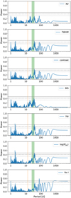 |
Fig. 4 Periodograms of the ESPRESSO radial velocities (top) and activity indicators (second to bottom: CCF FWHM, CCF contrast, CCF bisector, Hα , log R″HK , and Na I) for TOI-260. The vertical orange line indicates the candidate planet period; the green shaded area, 1σ around the stellar rotation period. The dotted, dashed, and solid horizontal grey lines indicate the 10%, 1%, and 0.1% FAP levels respectively. |
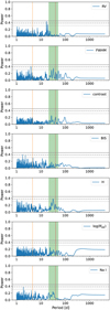 |
Fig. 5 Periodograms of the ESPRESSO radial velocities (top) and activity indicators (second to bottom: CCF FWHM, CCF contrast, CCF bisector, Hα, log R′HK, and Na I) for TOI-286. The vertical orange and red lines indicate the candidate planet periods for TOI-286.01 and TOI- 286.02. The green shaded area indicates 1σ around the stellar rotation period. The dotted, dashed, and solid horizontal grey lines indicate the 10%, 1%, and 0.1% FAP levels respectively. |
2.5.1 Gemini
We obtained speckle imaging observations from both Gemini South’s Zorro instrument and Gemini North’s ‘Alopeke instrument for TOI-260, and from Gemini South’s Zorro for TOI-286. Both instruments (Scott et al. 2021) provide simultaneous speckle imaging in two bands (562 nm and 832 nm) with output data products including a reconstructed image and robust contrast limits on companion detections (see Howell et al. 2011).
TOI-260 was observed on 12 September 2019 with ‘Alopeke at Gemini South and 12 October 2019 with Zorro at Gemini North. Both observations provided similar results, that TOI- 260 has no close companions to within the 5σ contrast limits obtained (5–8 magnitudes) and the angular limits sampled − 0.02 out to 1.2 arcsec (see Fig. 7). At the distance to TOI-260 of d = 20.2 pc, these angular limits correspond to 0.4 to 24 au.
TOI-286 was observed on 26 December 2020 with Zorro on Gemini North. The high-resolution observation showed that TOI-286 has no close companions to within the 5σ contrast limits obtained (5–9 magnitudes) and the angular limits sampled –0.02 out to 1.2 arcsec (see Fig. 8). At the distance to TOI-286 of d = 59.2 pc, these angular limits correspond to 1.2–71 au.
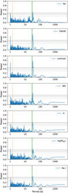 |
Fig. 6 Periodograms of the ESPRESSO radial velocities (top) and activity indicators (second to bottom: CCF FWHM, CCF contrast, CCF bisector, Hα , log R′HK , and Na I) for TOI-134. The vertical orange line indicates the published planetary period. The green shaded area indicates 1σ around the stellar rotation period. The dotted, dashed, and solid horizontal grey lines indicate the 10%, 1%, and 0.1% FAP levels respectively. |
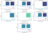 |
Fig. 7 Companion sensitivity for the near-infrared and optical adaptive optics imaging for TOI-260. Top to bottom and left to right: ’Alopeke at Gemini-North, Zorro at Gemini-South, NIRC2 at Keck, PHARO at Palomar, HRCam at SOAR, NESSI at WIYN (21 January 2019, 12 October 2019). For all observations save SOAR, the inset image(s) is of the primary target showing no additional close-in companions. For SOAR the inset image shows the auto-correlation function. |
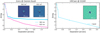 |
Fig. 8 Companion sensitivity for the adaptive optics imaging for TOI-286. Left: Gemini Zorro at Gemini-South, where the inset image is of the primary target at 562 nm and 832 nm, showing no additional close-in companions. Right: HRCam at SOAR, where the inset image shows the auto-correlation function. |
2.5.2 Palomar
The Palomar Observatory observations of TOI-260 were made with the PHARO instrument (Hayward et al. 2001) behind the natural guide star AO system P3K (Dekany et al. 2013) on 22 December 2018 in a standard 5-point quincunx dither pattern with steps of 5″ in the narrow-band Br-γ filter (λo = 2.1686; Δλ = 0.0326 µm). Each dither position was observed three times, offset in position from each other by 0.5″ for a total of 15 frames; with an integration time of 1.4 s per frame, the total on-source time was 21 seconds. PHARO has a pixel scale of 0.025″ per pixel for a total field of view of ~25″.
The science frames were flat-fielded and sky-subtracted. The flat fields were generated from a median average of dark subtracted flats taken on-sky. The flats were normalised such that the median value of the flats is unity. The sky frames were generated from the median average of the 15 dithered science frames; each science image was then sky-subtracted and flat-fielded. The reduced science frames were combined into a single combined image using a intra-pixel interpolation that conserves flux, shifts the individual dithered frames by the appropriate fractional pixels, and median-coadds the frames. The final resolution of the combined dithers was determined from the full-width half-maximum of the point spread function to be 0.105″.
To within the limits of the AO observations, no stellar companions were detected. The sensitivities of the final combined AO image were determined by injecting simulated sources azimuthally around the primary target every 20° at separations of integer multiples of the central source’s FWHM (Furlan & Howell 2017; Clark et al. 2024). The brightness of each injected source was scaled until standard aperture photometry detected it with 5σ significance. The resulting brightness of the injected sources relative to TOI-260 set the contrast limits at that injection location. The final 5σ limit at each separation was determined from the average of all of the determined limits at that separation and the uncertainty on the limit was set by the rms dispersion of the azimuthal slices at a given radial distance (see Fig. 7).
2.5.3 Keck
The Keck Observatory observations of TOI-260 were made with the NIRC2 instrument on Keck-II behind the natural guide star AO system (Wizinowich et al. 2000) on 9 September 2020 in the standard 3-point dither pattern that is used with NIRC2 to avoid the left lower quadrant of the detector which is typically noisier than the other three quadrants. The dither pattern step size was 3″ and was repeated twice, with each dither offset from the previous dither by 0.5″. NIRC2 was used in the narrow-angle mode with a full field of view of ~10″ and a pixel scale of approximately 0.0099442″ per pixel. The Keck observations were made in the narrow-band Br-γ filter (λo = 2.1686; Δλ = 0.0326 µm) with an integration time in each filter of 0.18 second for a total of 1.6 seconds on target.
The frames were processed in the same way as described for the Palomar observations. The final resolution of the combined dithers was determined from the full-width half-maximum of the point spread function to be 0.050″. To within the limits of the AO observations, no stellar companions were detected. The contrast curve is shown in Fig. 7.
2.5.4 SOAR
The SOAR TESS survey (Ziegler et al. 2020) observes TESS planet candidate hosts with speckle imaging using the high-resolution camera (HRCam) imager on the 4.1-m Southern Astrophysical Research (SOAR) telescope at Cerro Pachón, Chile (Tokovinin 2018). TOI-260 was observed on 12 August 2019, while TOI-286 was observed on 18 February 2019. In both cases, no nearby sources were detected within 3″. The contrast curves and auto-correlation functions are shown in Figs. 7 and 8 respectively.
2.5.5 WIYN
The NN-Explore Exoplanet Stellar Speckle Imager (NESSI, Scott 2019), which is mounted on the 3.5m WIYN telescope at Kitt Peak, observed TOI-260 twice, on 21 January 2019 and 12 October 2019. NESSI simultaneously acquires data in two bands centre ed at 562 nm and 832 nm using high speed electron-multiplying CCDs (EMCCDs). We collected and reduced the data following the procedures described in Howell et al. (2011). The resulting reconstructed image achieved a contrast of Δmag ~ 6.5 at a separation of 1" in the 832 nm band for the observation of 21 January, and of Δmag ~ 6 for the observation of 12 October (see Fig. 7).
2.6 Limits on outer companions from global astrometry
TOI-286 (CD-60 8051) and TOI-260 (BD-10 47) have been observed by both the HIPPARCOS and Gaia global astrometry missions. It is therefore possible to inspect the latest versions of the catalogues of astrometric accelerations constructed by Brandt (2021) and Kervella et al. (2022) in order to probe for the existence of outer, massive companions. No statistically significant proper motion difference is found for either of the two stars. However, as both these stars are late-type and nearby, the limits that can be placed on the mass of an outer companion as a function of semi-major axis are rather interesting. Based on Kervella et al. (2022), it is possible to rule out the presence of a giant planet in the approximate interval of orbital separations between 3 and 10 au with Mp ≳ 0.6 MJup and Mp ≳ 0.3 MJup around TOI-286 and TOI-260, respectively.
3 Analysis
3.1 Stellar parameters
The parameters of the three host stars are given in Table 1. We obtained the stellar coordinates, proper motions, and parallaxes from the Gaia Data Release 3 (Gaia Collaboration 2016, 2023). To compute the atmospheric parameters from the ESPRESSO spectra, we performed spectral synthesis with the STEPARSYN code8 (Tabernero et al. 2022). STEPARSYN provides the effective temperature Teff, metallicity [Fe/H], surface gravity log ɡ, and broadening parameter vbroad, which accounts for both the macroturbulence ζ and the projected rotational velocity vsini. The first set of error bars corresponds to the internal errors alone. For a more realistic uncertainty on Teff, we adopt the 2% error floor of Tayar et al. (2022), reported in brackets in Table 1.
As an independent comparison and validation, we also computed the atmospheric parameters through measurement of the equivalent widths of specific lines. For TOI-286, which is an early K dwarf, we used the ARES+MOOG approach described in Sousa (2014). TOI-134 and TOI-260 are cooler stars – an M dwarf and a late K dwarf – for which this approach is not suitable. Instead, we used the ODUSSEAS tool (Antoniadis-Karnavas et al. 2020), developed specifically for M dwarfs, although we note that TOI-260, which is on the K-M boundary, is on the edge of the temperature validity range. The parameters obtained for TOI-286 (Teff = 5059 ± 78 K), log ɡ = 4.50 ± 0.04 dex, [Fe/H] = −0.09 ± 0.05 dex) and TOI-134 (Teff = 3850 ± 91 K, log ɡ = 4.44 ± 0.08 dex, ([Fe/H] = -0.01 ± 0.11 dex) are generally compatible with those obtained from STEPARSYN. For TOI-260, they differ more notably (Teff = 3851 ± 101 K, log ɡ = 4.61 ± 0.06 dex, [Fe/H] = 0.06 ± 0.13 dex); this is most likely due to the star being indeed too hot for ODUSSEAS.
We also calculate the bolometric luminosities, masses, and radii. The bolometric luminosity Lbol is obtained by integrating the observed spectral energy distributions (SEDs), which are shown in Fig. 9 together with the best-fit Bt-Settle models from Allard et al. (2013). We note that the GALEX filters were removed from the SED integration, as only photospheric fluxes are relevant to the Lbol determination. The stellar radius R★ is obtained by using the Stefan-Boltzmann equation, which requires the Lbol and Teff. The stellar mass M★ is then obtained following the Schweitzer et al. (2019) mass-radius relationship for TOI-260 and TOI-134, and following the Eker et al. (2015) mass–luminosity relationship for TOI-286. The stellar density is calculated from M★ and R★. Our errors for these parameters are consistent with those expected by Tayar et al. (2022).
Additionally, we computed the Galactic space–velocity components U, V, and W using the Gaia DR3 proper motion, parallax and radial velocity, following the prescription of Johnson & Soderblom (1987). U is in the direction of the Galactic centre, V in the direction of Galactic rotation, and W in the direction of the north Galactic pole. We note that the right-handed system is used, and that we do not subtract the solar motion. Kinematically, TOI-286 belongs to the young disk, but it does not appear to be a member of any known young moving group.
Finally, we report the median and standard deviation of the log  activity indicator obtained from the ESPRESSO spectra for each target. From the log
  , we can estimate the stellar rotation period Prot. For TOI-260 and TOI-286, we use the log
  relation of Suárez Mascareño et al. (2015). For the cooler M dwarf TOI-134, we use the log
  activity relation of Astudillo-Defru et al. (2017).
Stellar parameters of TOI-260, TOI-286, and TOI-134.
3.2 Data modelling
We modelled the photometric and RV data simultaneously with the juliet9 software (Espinoza et al. 2019). juliet enables the joint fitting of transit and RV data, through the batman package (Kreidberg 2015) and the radvel package (Fulton et al. 2018) respectively. It also incorporates Gaussian process regression (GPR) via the celerite package (Foreman-Mackey et al. 2017). Importance nested sampling, using the dynesty package (Speagle 2020), is employed to explore the parameter space. By default, juliet adopts random walk sampling with 500 live points.
For each candidate transiting planet, we tested both circular and free-eccentricity models, fitting all the data simultaneously. Joint transit and RV fits in juliet require the stellar density ρ, and the following parameters for each planet pi: period Ppi, time of transit t0,pi, planet-to-star radius ratio ppi, impact parameter bpi, and either eccentricity epi and angle of periastron ωpi or a derived parametrisation such as  sin ωpi,
  cos ωpi. There are also intrumental parameters: for each RV instrument, the systemic radial velocity µinstrument and the jitter σw,instrument; for each photometric instrument, the dilution factor mdilution,instrument, the flux offset mflux,instrument, the jitter σ w,instrument, and the limb-darkening parameters q1,instrument and q2,instrument for the quadratic law parametrisation of Kipping (2013). We also used GPs to model the effect of stellar activity on the radial velocities and instrumental effects on the photometry. For the RVs, we use the quasi-periodic kernel (called exp-sine-squared kernel in juliet) of Haywood et al. (2014) . For the photometry, we employ the (approximate) Matern 3/2 kernel, as implemented in celerite.
From the juliet fitted parameters and the stellar parameters we derived for each planet the semimajor axis api, the mass Mpi, the radius Rpi, the density ρpi, and the equilibrium temperature Teq,pi. For this last we assume a Bond albedo of 0 and instant heat redistribution. The errors on the derived parameters are computed through error propagation, where for Teff we take the error floor from Tayar et al. (2022). The details of the fits for each star are discussed in the following subsections.
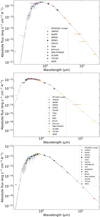 |
Fig. 9 Top: SED for TOI-260. The grey line shows the BT-Settl model for Teff = 3800K, solar metallicity, and log 𝑔 = 5.0 dex. Middle: SED for TOI-286. The grey line shows the BT-Settl model for Teff = 5100 K, solar metallicity, and log 𝑔 = 4.5 dex. Bottom: SED for TOI-134. The grey line shows the BT-Settl model for Teff = 3600 K, solar metallicity, and log 𝑔 = 4.5 dex. |
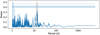 |
Fig. 10 Periodogram of the TOI-260 ESPRESSO RVs with a GP component removed. The semitransparent orange line indicates the period of the transiting candidate, at which there is a clear signal. |
3.2.1 TOI-260
We use ESPRESSO and HIRES RVs and TESS photometry to characterise the planetary candidate TOI-260.01. The ESPRESSO RVs do not immediately show evidence for a planet at the TESS candidate period of P ≈ 13.48 d, as can be seen in the periodogram in Fig. 4. However, most of the activity indicators show a strong signal at ≈37 d, which is also present in the RVs and which is close to the stellar rotation period, suggesting the stellar activity-induced variability may be overpowering the planet signal. To test this, we fitted a model consisting of a Keplerian signal and GP to the ESPRESSO RVs alone. In order to detrend the radial velocities from the stellar activity, we first fitted a GP to the FWHM activity indicator time series, which has previously shown to be a good tracer of stellar activity in ESPRESSO data (Lillo-Box et al. 2020; Lavie et al. 2023; Castro-González et al. 2023). We used broad log-uniform priors of 𝓙(0.001, 1000) for σGP,FWHM , αGP,FWHM , and ΓGP,FWHM , and a normal prior of 𝓝(31, 6) for the rotation period GP hyperparameter Prot,GP,FWHM, taking the value and uncertainty of the rotation period (see Sect. 3.1) as the mean and standard deviation for this last. Subsequently, we used the resulting parameters as priors on the radial velocity GP. The periodogram of the RVs with the GP component removed is shown in Fig. 10; a clear signal is evident at the planetary period.
For the rest of the analysis, we jointly fitted the ESPRESSO RVs, the HIRES RVs, and the TESS photometry. We tested two models: a circular transiting planet, and a transiting planet with free eccentricity. To detrend the RVs from stellar activity, we fit GPs to the HIRES data, and to the joint ESPRESSO data. We chose to use separate GPs both because these are different instruments, and because the ≈2000 d gap between the observations means that we are likely tracing different parts of the star’s activity cycle. However, we set the rotation period hyperparameter to be shared between the two GPs. We also tested a fit with a global GP on the RVs, with priors constrained by the SMW indicators, but obtained no improvement in the Bayesian log-evidence and a much larger resulting jitter for ESPRESSO. We constrained the priors for these GPs using activity indicators; for the ESPRESSO data we used the FWHM, as previously described. For HIRES we have fewer indicators available, as it is an iodine cell spectrograph and therefore the RVs are not calculated via the CCF method. We selected the SMW activity indicator and used the same procedure. The GP fits to these activity indicators are shown in Fig. B.1 in the online appendices10.
For the TESS photometry we employed a two-step process, where we first masked the transits and fitted GPs to the out-of-transit data only on a sector-by-sector basis, with broad log-uniform or Jeffreys priors of 𝓙(1 × 10−6,1 × 106) for σGP,sector and 𝒥(0.2,1 × 103) for ρGP,sector, where 𝒥(a, b) indicates a log-uniform distribution between a and b. We then used the resulting parameters as priors for GPs on the joint full fit of the RVs and all photometric data.
The ground-based photometry, taken after the TESS sector 3 observations with preliminary ephemerides, is unfortunately not in transit according to the refined ephemerides obtained from the modelling of the full TESS dataset and radial velocities (see Fig. 2). In any case, the observations were optimised for vetting faint nearby stars, so the scatter of the lightcurves for TOI-260 itself is too high to detect the transit. We therefore do not include the ground-based photometry in the modelling.
The priors and posteriors for the final models are given in Tables 2 and 3, for the circular fit and the free-eccentricity fit respectively. The cornerplots of the posterior distributions are shown in online appendix Figs. E.1, E.2, and E.3 for the circular fit; and in Figs. E.4, E.5, and E.6 for the free-eccentricity fit. In the prior distributions, 𝒰(a, b) indicates a uniform distribution between a and b; 𝒩(a, b) a normal distribution with mean a and standard deviation b; 𝒯𝒩(a, b, c, d) a truncated normal distribution with mean a, standard deviation b, and support in the [c, d] interval; 𝒥(a, b) a Jeffreys or log-uniform distribution between a and b. We used the values reported on ExoFOP as priors for the period Pp1, time of transit t0,p1, and planet-to-star radius ratio pp1.
Since we are using the PDC-SAP TESS light curves, we can expect that most of the variability in the TESS fluxes comes from instrumental systematics, which may vary between sectors. We therefore treat each TESS sector as an individual instrument with separate priors for the flux offsets mflux,sector and jitters σsector. Likewise, the GP priors σGP,sector and ρGP,sector are set individually, with priors given by the previous separate fits on the out-of-transit data. juliet also requires priors for the dilution factor, which we have fixed to 1 for all TESS sectors. The limb-darkening parameters q1,TESS and q2,TESS, however, are common to all TESS sectors.
For the radial velocity offsets µinstrument we used broad uniform priors spanning the range of the obtained RVs for each instrument. For the RV GPs, we used the posteriors of the GP fits to the FWHM and SMW activity indicator as priors for ESPRESSO and HIRES respectively (in the case of σGP,rv, scaled by a normalisation factor corresponding to the RV variation over the FWHM or SMW variation). For the free-eccentricity fit, we used the  parametrisation, and fixed an upper limit on the eccentricity of 0.7, to avoid convergence problems with batman at high eccentricities.
The Bayesian log-evidence comparison of the two models strongly favours the eccentric model (henceforth model e) over the circular model (henceforth model c), with ∆ log Zc−e ≈ 6. This model has a remarkably high eccentricity of  . However, it appears to be at least partly driven by a single ESPRESSO19 data point in an otherwise unsampled by ESPRESSO gap in phase coverage in the (−0.1,0) phase range, that is also poorly covered by HIRES. Additionally, the cornerplot (online appendix Fig. E.4) suggests the posterior for
  parameter is at the edge of the prior space. Therefore, we ran other models for comparison: two models using the
  parametrisation, one with a limiting eccentricity of 0.9 (model e1), and one with a limiting eccentricity of 0.5 (model e2), to explore the impact of this limit; one model using the (e, ω) parametrisation (model e3), with a log-uniform prior on e between 0.001 and 0.9; and one model using the initial
  parametrisation and 0.7 eccentricity limit, but with the ESPRESSO19 data point that appears to be driving the eccentricity removed (model e4). Model e1 returns an even higher eccentricity of ep1 = 0.80 ± 0.05, although with ∆ log Ze−e1 ≈ 3 in favour of model e, and a better-sampled posterior for
  . Model e2 returns a more poorly constrained eccentricity of
  , and is not favoured by the log-evidence comparison with the initial model (∆ log Ze−e2 ≈ 5), though the posterior distributions do not appear visually poorly sampled. Meanwhile, model e3 returns a similarly high and more poorly constrained eccentricity of
  , with ∆ log Ze−e3 ≈ 4 in favour of the initial free-eccentricity model e. Finally, model e4 returns a slightly lower (though still compatible within error bars) and less constrained eccentricity to model e of
  . A ∆ log Z comparison is not appropriate here since the input data is different.
We therefore conclude that the current ESPRESSO data do not allow us to properly constrain the eccentricity of the orbit, and thus prefer the simpler circular model. We also note that one mechanism for driving such a high eccentricity would be through interactions with other planets, but we see no evidence for outer companions in the RVs, and the astrometric data places limits on the existence of massive outer companions (see Sect. 2.6). We show the RVs and median circular model in Fig. 11, and the phase-folded stacked TESS data and model in Fig. 12. The full TESS light curves and corresponding median models are shown in online appendix Fig. C.1. With the circular model, we find an RV semi-amplitude of  ms−1, corresponding to a detection at 3σ, and leading to a planetary mass of Mp1 = 4.23 ± 1.60 M⊕.
Prior and posterior planetary parameter distributions for TOI-260, for a fit with eccentricity fixed to 0.
Prior and posterior planetary parameter distributions for TOI-260, for the free-eccentricity model.
3.2.2 TOI-286
We use ESPRESSO and HARPS RVs and TESS photometry to characterise the planetary candidates TOI-286.01 and TOI-286.02. As with TOI-260, the ESPRESSO RVs for TOI-286 do not immediately show evidence for periodic signals at either of the TESS candidate periods of P ≈ 4.5 d and P ≈ 39.4 d, as can be seen in the periodogram in Fig. 5. The stellar activity indicators, however, show evidence for both a long-term trend and some signal at ≈32 d, close to the stellar rotation period determined from the log relations (see Sect. 3.1). To test whether the stellar activity is also masking the planetary signals for this target, we fitted a model consisting of two Keplerian signals and a GP to the ESPRESSO RVs alone. In order to detrend the radial velocities from the stellar activity, we first fitted a GP to the FWHM activity indicator time series. We used broad log-uniform priors of 𝒥(0.001, 1000) for σGP,FWHM, αGP,FWHM, and ΓGP,FWHM, and a normal prior of 𝒩(36, 15) for the rotation period GP hyperparameter Prot,GP,FWHM, taking the value and uncertainty of the rotation period (see Sect. 3.1) as the mean and standard deviation. Subsequently, we used the resulting parameters as priors on the radial velocity GP. The periodogram of the RVs with the GP component removed is shown in Fig. 13; a signal can be seen at the period of the inner candidate, but there is none at the period of the outer candidate. This is not unexpected, as it is close to the estimated stellar rotation period and is thus likely to be partly absorbed by the stellar activity GP unless both the activity and the planet are fitted simultaneously.
We therefore tested three models for the full fit of all the data acquired for TOI-286: a single circular transiting planet corresponding to the inner signal, two circular transiting planets, and two transiting planets with free eccentricity. Since the HARPS RVs are few and coeval with the start of the ESPRESSO18 data, we detrended the RVs using a global GP constrained by the GP on the ESPRESSO FWHM activity indicator. The GP fit to the FWHM is shown in online appendix Fig. B.1.
As it is in the TESS continuous viewing zone, TOI-286 has a wealth of TESS data that makes simultaneous modelling of the photometric instrumental parameters and GPs for all sectors together with the planet computationally prohibitive. Therefore, we employed a variation of the two-step process used for TOI-260, where we first masked the transits (with a margin of 5 hours around each transit window) and fitted GPs and instrumental parameters to the out-of-transit data only on a sector-by-sector basis, then fixed the resulting parameters for the joint full fit in which we employed only the in-transit TESS data. We report the priors and posteriors of the GP fits to the out-of-transit data in online Appendix D.
While the ground-based photometry is in transit, its main purpose was to vet nearby stars, particularly the companion at 17″ separation, and verify they are not background eclipsing binaries. The variation of the photometry is too high for the small transits measured by TESS to be detectable, so we do not include them in the full model.
The priors and posteriors of the three models are given in Table 4 for the one-planet model, Table 5 for the model with two circular planets, and Table 6 for the model with two planets with free eccentricities, respectively. The prior distributions were chosen in an analogous way to those for TOI-260, with the following differences: For the parameters of the outer candidate, period Pp2, time of transit t0,p2, and planet-to-star radius ratio pp2, we also use the ExoFOP values as priors. The TESS instrumental parameters for each sector are fixed in this case, other than the global limb-darkening parameters q1,TESS and q2,TESS. For the global RV GP, we used the posteriors of the GP fit to the FWHM activity indicator as priors (in the case of σGP,rv, scaled by a normalisation factor corresponding to the RV variation over the FWHM variation). For the free-eccentricity fit, we used the  parametrisation for both planets, and fixed an upper limit on the eccentricities of 0.7. The cornerplots of the posterior distributions are shown in online appendix Figs. E.7 and E.8 for the one-planet fit; in Figs. E.9, E.10, and E.11 for the two-planet circular fit; and in Figs. E.12, E.13, and E.14 for the free-eccentricity fit.
The log-evidence comparison of the three models very strongly favours the two-planet models over the one-planet model, with ∆ log Z ≈ 769 for both two-planet models versus the one-planet circular model. Comparison between the two 2-planet models slightly favours the model with circular orbits, with ∆ log Z ≈ 2.9, although the difference in log-evidence is only marginally significant; therefore, we prefer the simpler circular model. We also note that the eccentricities in the free-eccentricity model are low, with both being compatible with 0 at the 2σ level. We show the RVs and median circular model in Fig. 14, and the phase-folded stacked TESS data and model in Fig. 15. The full TESS light curves and corresponding median models are shown in online appendix Fig. C.2 for sector 1 as an illustration. With the circular model, we find for TOI-268 b an RV semi-amplitude of Kp1 = 1.98 ± 0.33 ms−1, corresponding to a detection at 3σ, and leading to a planetary mass of Mp1 = 4.67 ± 0.75 M⊕. The RV semi-amplitude found for TOI-286 c of  ms−1 is only marginally significant; it leads to a planetary mass of Mp1 = 3.72 ± 2.22 M⊕.
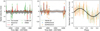 |
Fig. 11 Left and centre: radial velocities (HIRES, green dots; ESPRESSO18, blue dots; and ESPRESSO19, orange dots), model components (GP, red; and Keplerian, grey), and median circular model (black) for TOI-260. We have separated the RVs into two plots for ease of viewing, as there is a ≈2000d gap between the HIRES and ESPRESSO RVs. The error bars show the RV errors and jitter added in quadrature. The instrumental systemic velocity has been subtracted. The GP fits to the SMW and FWHM activity indicators are also shown (dotted green lines) for comparison. Right: phase-folded radial velocities plus median Keplerian, following the same colour scheme. |
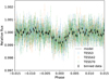 |
Fig. 12 Stacked phase-folded TESS data for TOI-260 with the median circular model (grey line). The points show the data from sectors 3 (blue), 42 (orange) and 70 (green), and binned data (black points). |
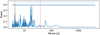 |
Fig. 13 Periodogram of the TOI-286 ESPRESSO RVs with a GP component removed. The orange and red semitransparent lines indicate the periods of the two transiting candidates. The strongest signal in the peri-odogram is located at the period of the inner candidate, but there is none at the period of the outer candidate. |
Prior and posterior planetary parameter distributions for TOI-286, for a one-planet circular model.
3.2.3 TOI-134
The transiting super-Earth TOI-134 b was first confirmed by Astudillo-Defru et al. (2020), using TESS photometry and HARPS and Magellan/PFS RVs. The orbital parameters were subsequently updated by Patel & Espinoza (2022). In this work, we present refined values of the planetary parameters based on ESPRESSO observations in addition to the published HARPS and PFS RVs, and additional TESS data. We tested two models: a circular transiting planet, and a transiting planet with free eccentricity.
The periodograms of the ESPRESSO data in Fig. 6 show a very strong signal at ≈31 d in the activity indicators and RV alike. The RVs will therefore require detrending from the stellar activity. Unfortunately, only two activity indicators are available for all four instruments, Hα, and S MW, and their values are not consistent from one instrument to another. However, the HARPS, PFS, and ESPRESSO18 RVs are roughly coeval, and the ESPRESSO19 RVs are close in time to them. We therefore chose to use a global RV GP, since it should be modelling the same underlying stellar activity. To constrain the parameters, we first fitted a GP to the FWHM activity indicator time series of the ESPRESSO data, and used the resulting parameters as priors on the RV GP. This GP fit is shown in online appendix Fig. B.1. For the TESS photometry we employed the same two-step process as for TOI-260.
The priors and posteriors are given in Tables 7 and 8 for the fixed-eccentricity and free-eccentricity fits, respectively. The prior distributions were chosen similarly to those for TOI-260, except that we used the published orbital parameters as priors. The cornerplots of the posterior distributions are shown in online appendix Figs. E.15, E.16, and E.17 for the circular fit; and in Figs. E.18, E.19, and E.20 for the free-eccentricity fit.
The log-evidence comparison of the two models slightly favours the eccentric model, with ∆ log Z ≈ 2.6. However, the difference is only marginally significant, and the eccentricity of the free-eccentricity fit is very small and compatible with zero at the 2σ level. Therefore, we adopt the circular model. We show the RVs and median circular model in Fig. 16, and the phase-folded stacked TESS data and model in Fig. 17. The full TESS light curves and corresponding median models are shown in online appendix Fig. C.3.
Prior and posterior planetary parameter distributions for TOI-286, for two circular planets.
Prior and posterior planetary parameter distributions for TOI-286, for two planets with free eccentricity.
4 Discussion
4.1 Update to the parameters of TOI-134
The goal of our analysis of TOI-134 was to update and refine the planetary parameters from Astudillo-Defru et al. (2020) (henceforward AD20) and Patel & Espinoza (2022) (henceforward PE22) with the more accurate ESPRESSO RVs, as well as additional TESS sectors (two compared to AD20, one compared to PE22). Table 9 lists the main orbital and physical parameters we compare. While all the reported orbital periods are equivalent at the 1σ level, we improve the precision on the period by a factor of ~200 compared to AD20. We also constrain the orbit to circularity. Regarding the physical parameters of the planet, we find a slightly lower mass, with improved precision, though it remains compatible with the value of AD20 at the 2σ level. We also find a slightly larger radius ratio than both AD20 and PE22. The larger radius and lower mass combined lead to a notably lower density for TOI-134 b than that reported by AD20. We note that this is robust to the stellar parameter determination; our stellar mass and radius are compatible with those of AD20 within error bars, and computing the planetary mass and radius with radius and mass with their stellar parameters leads to an even lower planetary density.
4.2 Planet composition
Knowing both the mass and radius of a planet allows us to compute its density, and compare it to composition models. Figure 18 shows the four planets presented in this paper, in the context of both compositional models and the population of well-characterised small, low-mass planets around similar stellar hosts. The planets are taken from the PlanetS catalogue. The compositional models are from Zeng et al. (2019)11.
For TOI-260 b, considering its 4.23 ± 1.60 M⊕ mass and 1.71 ± 0.08 R⊕ radius from the circular model, the most likely composition is between a pure rock planet, and a rocky core with a 50% condensed water layer. However, the large uncertainty on the mass (primarily due to the large relative uncertainty on the RV semi-amplitude) makes a clear determination challenging. The uncertainty on the eccentricity is also important here; if the high-eccentricity model is actually correct, we obtain a much higher mass. In this case, the most likely composition would be between a pure iron and a half-iron, half-silicates model.
The two planets orbiting TOI-286 have similar masses, but notably different radii, leading to different probable compositions. The inner, hotter, smaller planet TOI-286 b, with a 4.53 ± 0.78 M⊕ mass and 1.42 ± 0.10 R⊕ radius, is likely close to a 50% iron core and 50% silicate mantle, or an Earth-like composition. The cooler, outer, larger planet TOI-286 c should have a higher volatile content considering its 3.72 ± 2.22 Me mass and i.88 ± 0.i2Re radius, and most likely has a significant water layer. Considering their bulk densities (normalised by the scaled Earth bulk density), these planets likewise sit on either side of the density gap proposed by Luque & Pallé (2022), with TOI-286 b being consistent with the rocky planet population, and TOI-286 c with the water worlds. This in turn suggests that TOI-286 b likely formed within the snow line, while TOI-286 c would have formed beyond it and migrated inwards (Luque & Pallé 2022, and references therein).
Our updated parameters for TOI-134 b suggest a pure rock composition. This contrasts with the results of AD20, who obtained a density more compatible with a 50% iron core and 50% silicate mantle.
Two of our planets – TOI-260 b and TOI-286 c – fall within the Fulton radius gap or radius valley (Fulton et al. 2017), with radii between 1.5 R⊕ and 2 R⊕. The precise location of the radius valley has been shown to depend on orbital period (Martinez et al. 2019) and stellar type (Cloutier & Menou 2020; Venturini et al. 2024). Using the period-radius relation of Cloutier & Menou (2020), we find the centre of the valley at 1.64 R⊕ at the period of TOI-260 b, and at 1.70 R⊕ at the period of TOI-286 c. TOI-260 b, with a radius of 1.71 ± 0.08 R⊕, is thus close to the centre of the valley, while TOI-286 c, with a radius of 1 . 88 ± 0.12 R⊕, is close to the upper border. Likewise, using the stellar mass-planet radius relation of Venturini et al. (2024), we find the centre of the valley at 1.70 R⊕ at the stellar mass of TOI-260, and at 1.77 R⊕ at the stellar mass of TOI-286. Again, this places TOI-260 b in the centre of the valley, and TOI-286 c towards the upper part. The normalised bulk density of TOI-260 b suggests it is most likely a rocky world formed within the snow line, potentially in situ (Venturini et al. 2020a,b; Luque & Pallé 2022; Burn et al. 2024). However, given the error bars on the mass and the uncertainty regarding the eccentricity, we cannot exclude a water-rich composition for this planet, and thus a formation beyond the snow line. Meanwhile, given both its location in the upper part of the radius valley and its bulk density, TOI-286 c is likely water-rich. The TOI-286 system thus has one rocky planet below the radius gap and one water-rich planet close to the upper border orbiting the same star. This is a similar configuration to the TOI-238 system, also consisting of two planets – an inner rocky planet and an outer water-rich planet – orbiting a K dwarf (Suárez Mascareño et al. 2024). Systems such as these are highly valuable probes of the radius gap.
In addition to comparing with theoretical composition curves, we can also use interior inference models to characterise the interior structure of our planets. We employ the ExoMDN code (Baumeister & Tosi 2023)12 to model our planets using a four-layer model consisting of an iron core, a silicate mantle, a water layer, and a H/He atmosphere. The inputs to ExoMDN are the planet’s mass, radius, and equilibrium temperature. We include both the circular and eccentric models for TOI-260 b. The resulting models are shown in Fig. A.1, together with a model of the Earth for comparison. The circular model for TOI-260 b has higher mantle and water radius fractions compared to the eccentric model, which is more similar to the Earth model proportions, though with a larger core fraction and lower mantle fraction. Regarding the TOI-286 system, TOI-286 b is strongly core-dominated, while TOI-286 c has a significant water radius fraction. Finally, the proportions of the model for TOI-134 b are similar to that of the Earth model.
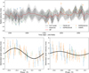 |
Fig. 14 Top: radial velocities (ESPRESSO18, blue dots; ESPRESSO19, orange dots; and HARPS, green dots), model components (GP, red; and Keplerian, grey), and median circular model (black) for TOI-286. The error bars show the RV errors and jitter added in quadrature. The instrumental systemic velocity has been subtracted. The GP fit to the FWHM activity indicator is also shown (dotted green line) for comparison. Bottom: phase-folded radial velocities plus median Keplerian for the inner (left) and outer (right) candidates, following the same colour scheme. |
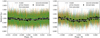 |
Fig. 15 Stacked phase-folded TESS data for TOI-286 with the median circular model (grey line), for the inner candidate (left) and outer candidate (right). The points show the data from the TESS primary mission (blue), first extended mission (orange), and second extended mission (green), and binned data (black points). |
Prior and posterior planetary parameter distributions for TOI-134, for a fit with eccentricity fixed to 0.
Prior and posterior planetary parameter distributions for TOI-134, for a fit with free eccentricity.
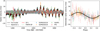 |
Fig. 16 Left: radial velocities (ESPRESSO18, blue dots; ESPRESSO19, orange dots; HARPS, green dots; and PFS, red dots), model components (GP, red; and Keplerian, grey), and median circular model (black) for TOI-134. The error bars show the RV errors and jitter added in quadrature. The instrumental systemic velocity has been subtracted. The GP fit to the FWHM activity indicator for ESPRESSO is also shown (dotted green line) for comparison. Right: phase-folded radial velocities plus median Keplerian, following the same colour scheme. |
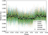 |
Fig. 17 Stacked phase-folded TESS data for TOI-134 with the median circular model (grey line). The points show the data from sectors 1 (blue), 28 (orange) and 68 (green), and binned data (black points). |
Parameter comparison for TOI-134.
4.3 Orbital parameters
To place our planets in a population context in regard to orbital parameters, we plot in Fig. 19 the period-eccentricity distribution of the small, well-characterised planets around low-mass stellar hosts. Of these planets, slightly under half (45%) have tabulated eccentricities of 0, as is the case for the planets presented here. However, the majority have low eccentricities, with 86% being below 0.1. The relatively few planets with higher eccentricities are preferentially found at longer periods above ≈3 d. If the eccentric model for TOI-260 b should prove to be correct, it would be by far the most eccentric such planet known.
The prevailing low eccentricities of this population contrast with the nonzero eccentricities found for warm Neptunes by Correia et al. (2020). These raised eccentricities are suggested to be a product of the same combination of high-eccentricity migration and atmospheric evaporation that sculpts the hot Neptune desert (Owen & Lai 2018), where atmospheric evaporation could excite the eccentricities through thermal tidal torque. Regarding the high-eccentricity model for TOI-260 b, since both mechanisms produce similar lower boundaries for the desert, we cannot exclude either of them as a potential originator.
All our planets are among the lower-mass part of the population. TOI-286 c, in particular, is the lowest-mass planet of this population at its orbital period.
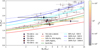 |
Fig. 18 Mass-radius diagram for all planets in the PlanetS catalogue with Rp < 3 R⊕ and Mp < 15 M⊕, well-constrained masses and radii (5% error on radius, 25% error on mass), hosted by early M and K stars (0.35 M⊙ < Ms < 0.9 M⊙). The points are coloured by Teq. The four planets presented in this paper are highlighted. We also show the eccentric solution for TOI-260 b, and the previous solution from AD20 for TOI-134 b (overlapped by TOI-286 b). The coloured curves show the composition models of Zeng et al. (2019). |
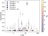 |
Fig. 19 Period-eccentricity diagram for the same population of planets as Fig. 18. The points are coloured by planet mass. The four planets presented in this paper are highlighted. We also show the eccentric solution for TOI-260 b. |
4.4 Atmospheric characterisation potential
To assess the potential of these planets for atmospheric characterisation, we computed the transmission spectroscopy metric (TSM) and emission spectroscopy metric (ESM) as defined by Kempton et al. (2018). For TOI-260 b we obtain a TSM of ~70.5 and an ESM of ~3.1. For TOI-286 b and c we find TSM values of ~4.1 and ~37.4 respectively, and ESM values of ~2.9 and ~0.7 respectively. Finally, for TOI-134 b we obtain a TSM of ~94.7 and an ESM of ~13.8. Regarding transmission spectroscopy, none of the newly confirmed planets reach the thresholds proposed by Kempton et al. (2018) of 10 for small planets (Rp ≤ 1.5 R⊕) or 90 for larger planets. TOI-134 b, however, surpasses the threshold, making it a promising candidate for transmission spectroscopy. This contrasts with the low TSM computed by Astudillo-Defru et al. (2020); the difference is primarily due to the larger radius we find. Regarding emission spectroscopy, once again the newly confirmed planets are below the 7.5 threshold of Kempton et al. (2018). On the other hand, TOI-134 b surpasses it and is thus also a promising candidate for characterisation in emission, as was previously noted by Astudillo-Defru et al. (2020).
5 Conclusions
We have presented the confirmation and characterisation of three new super-Earths:
TOI-260 b, the only known planet around TOI-260, with an orbital period of
 d. It has a 4.23 ± 1.60 M⊕ mass and a 1.71 ± 0.08 R⊕ radius, suggesting a rocky composition with a water layer. The eccentricity of this planet is poorly constrained; further observations would be needed to better evaluate it;
TOI-286 b, a
 d planet with a 4.53 ± 0.78 M⊕ mass and 1.42 ± 0.10 R⊕ radius, suggesting an earthlike composition and thus a formation within the snowline;
TOI-286 c, a
 d planet with a 3.72 ± 2.22 M⊕ mass and 1.88 ± 0.12 R⊕ radius, suggesting a significant water layer and therefore a formation outside the snowline.
We also updated and refined the parameters of TOI-134 b, finding a lower mass and larger radius compared to the literature, that point to a rocky composition.
Acknowledgements
We thank the referee for their helpful comments and careful reading that improved this manuscript. We thank the Swiss National Science Foundation (SNSF) and the Geneva University for their continuous support to our planet low-mass companion search programmes. This work has been carried out within the framework of the National Centre of Competence in Research PlanetS supported by the Swiss National Science Foundation. This publication makes use of The Data & Analysis Center for Exoplanets (DACE), which is a facility based at the University of Geneva (CH) dedicated to extrasolar planets data visualisation, exchange and analysis. DACE is a platform of the Swiss National Centre of Competence in Research (NCCR) PlanetS, federating the Swiss expertise in Exoplanet research. The DACE platform is available at https://dace.unige.ch. This work made use of tpfplotter by J. Lillo-Box (publicly available in www.github.com/jlillo/tpfplotter), which also made use of the python packages astropy, lightkurve, matplotlib and numpy. This research has made use of the Exoplanet Follow-up Observation Program (ExoFOP; DOI: 10.26134/ExoFOP5) website, which is operated by the California Institute of Technology, under contract with the National Aeronautics and Space Administration under the Exoplanet Exploration Program. Based on observations carried out at the European Southern Observatory (ESO; La Silla, Chile) using the 3.6m telescope, under ESO programmes 1102.C-0923(A), 1102.C-0249(A), and 60.A-9700(G). The observations in the paper made use of the NN-EXPLORE Exoplanet and Stellar Speckle Imager (NESSI). NESSI was funded by the NASA Exoplanet Exploration Program and the NASA Ames Research Center. NESSI was built at the Ames Research Center by Steve B. How-ell, Nic Scott, Elliott P. Horch, and Emmett Quigley. The authors are honored to be permitted to conduct observations on Iolkam Du’ag (Kitt Peak), a mountain within the Tohono O’odham Nation with particular significance to the Tohono O’odham people. Some of the observations in this paper made use of the High-Resolution Imaging instruments ‘Alopeke and Zorro and were obtained under Gemini LLP Proposal Number: GN/S-2021A-LP-105. ‘Alopeke and Zorro were funded by the NASA Exoplanet Exploration Program and built at the NASA Ames Research Center by Steve B. Howell, Nic Scott, Elliott P. Horch, and Emmett Quigley. Both instruments were mounted on the Gemini North/South telescopes of the international Gemini Observatory, a program of NSF’s OIR Lab, which is managed by the Association of Universities for Research in Astronomy (AURA) under a cooperative agreement with the National Science Foundation. on behalf of the Gemini partnership: the National Science Foundation (United States), National Research Council (Canada), Agencia Nacional de Investigación y Desarrollo (Chile), Ministerio de Ciencia, Tecnología e Innovación (Argentina), Ministério da Ciência, Tecnologia, Inovações e Comu-nicações (Brazil), and Korea Astronomy and Space Science Institute (Republic of Korea). Funding for the TESS mission is provided by NASA’s Science Mission Directorate. KAC acknowledges support from the TESS mission via subaward s3449 from MIT. This paper made use of data collected by the TESS mission and are publicly available from the Mikulski Archive for Space Telescopes (MAST) operated by the Space Telescope Science Institute (STScI). We acknowledge the use of public TESS data from pipelines at the TESS Science Office and at the TESS Science Processing Operations Center. Resources supporting this work were provided by the NASA High-End Computing (HEC) Program through the NASA Advanced Supercomputing (NAS) Division at Ames Research Center for the production of the SPOC data products. This work makes use of observations from the LCOGT network. Part of the LCOGT telescope time was granted by NOIRLab through the Mid-Scale Innovations Program (MSIP). MSIP is funded by NSF. JIGH, RR, CAP and ASM acknowledge financial support from the Spanish Ministry of Science and Innovation (MICINN) project PID2020-117493GB-I00. This work was financed by Portuguese funds through FCT (Fundação para a Ciência e a Tecnologia) in the framework of the project 2022.04048.PTDC (Phi in the Sky, DOI 10.54499/2022.04048.PTDC). C.J.M. also acknowledges FCT and POCH/FSE (EC) support through Investi-gador FCT Contract 2021.01214.CEECIND/CP1658/CT0001. We acknowledge financial support from the Agencia Estatal de Investigación of the Ministerio de Ciencia e Innovación MCIN/AEI/10.13039/501100011033 and the ERDF “A way of making Europe” through project PID2021-125627OB-C32, and from the Centre of Excellence “Severo Ochoa” award to the Instituto de Astrofisica de Canarias. FPE and CLO would like to acknowledge the Swiss National Science Foundation (SNSF) for supporting research with ESPRESSO through the SNSF grants nos. 140649, 152721, 166227, 184618 and 215190. The ESPRESSO Instrument Project was partially funded through SNSF’s FLARE Programme for large infrastructures. Funded/Co-funded by the European Union (ERC, FIERCE, 101052347). Views and opinions expressed are however those of the author(s) only and do not necessarily reflect those of the European Union or the European Research Council. Neither the European Union nor the granting authority can be held responsible for them. This work was supported by FCT – Fundação para a Ciência e a Tecnologia through national funds and by FEDER through COM-PETE2020 – Programa Operacional Competitividade e Internacionalização by these grants: UIDB/04434/2020; UIDP/04434/2020. S.G.S. acknowledges the support from FCT through Investigador FCT contract no. CEECIND/00826/2018 and POPH/FSE (EC). This work has made use of data from the European Space Agency (ESA) mission Gaia (https://www.cosmos.esa.int/gaia), processed by the Gaia Data Processing and Analysis Consortium (DPAC, https://www.cosmos.esa.int/web/gaia/dpac/consortium). Funding for the DPAC has been provided by national institutions, in particular the institutions participating in the Gaia Multilateral Agreement. A.S.M. acknowledges financial support from the Spanish Ministry of Science and Innovation (MICINN) project PID2020-117493GB-I00 and from the Government of the Canary Islands project ProID2020010129. A.C.-G. and J.L.-B. are funded by the Spanish Ministry of Science through MCIN/AEI/10.13039/501100011033 grants PID2019-107061GB-C61 and CNS2023-144309. This research was funded in part by the UKRI (Grants ST/X001121/1, EP/X027562/1). This work has been carried out within the framework of the NCCR PlanetS supported by the Swiss National Science Foundation under grants 51NF40_182901 and 51NF40_205606. X.D. acknowledges the support from the European Research Council (ERC) under the European Union’s Horizon 2020 research and innovation programme (grant agreement SCORE No. 851555) and from the Swiss National Science Foundation under the grant SPECTRE (No 200021_215200).
Appendix A Additional figure
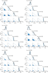 |
Fig. A.1 Cornerplots of the radius fractions of the four-layer interior structure models for (top to bottom, left to right): the circular model for TOI-260 b, the eccentric model for TOI-260 b, TOI-286 b, TOI-286 c, TOI-134 b, and Earth for comparison. |
References
- Akeson, R. L., Chen, X., Ciardi, D., et al. 2013, PASP, 125, 989 [Google Scholar]
- Allard, F., Homeier, D., Freytag, B., Schaffenberger, W., & Rajpurohit, A. S. 2013, Mem. Soc. Astron. Ital. Suppl., 24, 128 [Google Scholar]
- Aller, A., Lillo-Box, J., Jones, D., Miranda, L. F., & Barceló Forteza, S. 2020, A&A, 635, A128 [NASA ADS] [CrossRef] [EDP Sciences] [Google Scholar]
- Anglada-Escudé, G., & Butler, R. P. 2012, ApJS, 200, 15 [Google Scholar]
- Antoniadis-Karnavas, A., Sousa, S. G., Delgado-Mena, E., et al. 2020, A&A, 636, A9 [NASA ADS] [CrossRef] [EDP Sciences] [Google Scholar]
- Astudillo-Defru, N., Delfosse, X., Bonfils, X., et al. 2017, A&A, 600, A13 [NASA ADS] [CrossRef] [EDP Sciences] [Google Scholar]
- Astudillo-Defru, N., Cloutier, R., Wang, S. X., et al. 2020, A&A, 636, A58 [NASA ADS] [CrossRef] [EDP Sciences] [Google Scholar]
- Baranne, A., Queloz, D., Mayor, M., et al. 1996, A&AS, 119, 373 [NASA ADS] [CrossRef] [EDP Sciences] [Google Scholar]
- Baumeister, P., & Tosi, N. 2023, A&A, 676, A106 [NASA ADS] [CrossRef] [EDP Sciences] [Google Scholar]
- Bonfils, X., Mayor, M., Delfosse, X., et al. 2007, A&A, 474, 293 [NASA ADS] [CrossRef] [EDP Sciences] [Google Scholar]
- Brandt, T. D. 2021, ApJS, 254, 42 [NASA ADS] [CrossRef] [Google Scholar]
- Brown, T. M., Baliber, N., Bianco, F. B., et al. 2013, PASP, 125, 1031 [Google Scholar]
- Burn, R., Mordasini, C., Mishra, L., et al. 2024, Nat. Astron., 8, 463 [Google Scholar]
- Butler, R. P., Vogt, S. S., Laughlin, G., et al. 2017, AJ, 153, 208 [Google Scholar]
- Castro-González, A., Díez Alonso, E., Menéndez Blanco, J., et al. 2022, MNRAS, 509, 1075 [Google Scholar]
- Castro-González, A., Demangeon, O. D. S., Lillo-Box, J., et al. 2023, A&A, 675, A52 [NASA ADS] [CrossRef] [EDP Sciences] [Google Scholar]
- Ciardi, D. R., Beichman, C. A., Horch, E. P., & Howell, S. B. 2015, ApJ, 805, 16 [NASA ADS] [CrossRef] [Google Scholar]
- Cincunegui, C., Díaz, R. F., & Mauas, P. J. D. 2007, A&A, 469, 309 [NASA ADS] [CrossRef] [EDP Sciences] [Google Scholar]
- Clark, C. A., van Belle, G. T., Horch, E. P., et al. 2024, AJ, 167, 56 [NASA ADS] [CrossRef] [Google Scholar]
- Cloutier, R., & Menou, K. 2020, AJ, 159, 211 [NASA ADS] [CrossRef] [Google Scholar]
- Collins, K. A., Kielkopf, J. F., Stassun, K. G., & Hessman, F. V. 2017, AJ, 153, 77 [Google Scholar]
- Correia, A. C. M., Bourrier, V., & Delisle, J. B. 2020, A&A, 635, A37 [NASA ADS] [CrossRef] [EDP Sciences] [Google Scholar]
- Dekany, R., Roberts, J., Burruss, R., et al. 2013, ApJ, 776, 130 [CrossRef] [Google Scholar]
- Díaz, R. F., Cincunegui, C., & Mauas, P. J. D. 2007, MNRAS, 378, 1007 [Google Scholar]
- Eker, Z., Soydugan, F., Soydugan, E., et al. 2015, AJ, 149, 131 [Google Scholar]
- Espinoza, N., Kossakowski, D., & Brahm, R. 2019, MNRAS, 490, 2262 [Google Scholar]
- Foreman-Mackey, D., Agol, E., Ambikasaran, S., & Angus, R. 2017, AJ, 154, 220 [Google Scholar]
- Fressin, F., Torres, G., Charbonneau, D., et al. 2013, ApJ, 766, 81 [NASA ADS] [CrossRef] [Google Scholar]
- Fulton, B. J., Petigura, E. A., Howard, A. W., et al. 2017, AJ, 154, 109 [Google Scholar]
- Fulton, B. J., Petigura, E. A., Blunt, S., & Sinukoff, E. 2018, PASP, 130, 044504 [Google Scholar]
- Furlan, E., & Howell, S. B. 2017, AJ, 154, 66 [NASA ADS] [CrossRef] [Google Scholar]
- Gaia Collaboration (Prusti, T., et al.) 2016, A&A, 595, A1 [NASA ADS] [CrossRef] [EDP Sciences] [Google Scholar]
- Gaia Collaboration (Vallenari, A., et al.) 2023, A&A, 674, A1 [NASA ADS] [CrossRef] [EDP Sciences] [Google Scholar]
- Guerrero, N. M., Seager, S., Huang, C. X., et al. 2021, ApJS, 254, 39 [NASA ADS] [CrossRef] [Google Scholar]
- Hadjigeorghiou, A., & Armstrong, D. J. 2024, MNRAS, 527, 4018 [Google Scholar]
- Hayward, T. L., Brandl, B., Pirger, B., et al. 2001, PASP, 113, 105 [NASA ADS] [CrossRef] [Google Scholar]
- Haywood, R. D., Collier Cameron, A., Queloz, D., et al. 2014, MNRAS, 443, 2517 [Google Scholar]
- Høg, E., Fabricius, C., Makarov, V. V., et al. 2000, A&A, 355, L27 [Google Scholar]
- Howell, S. B., Everett, M. E., Sherry, W., Horch, E., & Ciardi, D. R. 2011, AJ, 142, 19 [Google Scholar]
- Jenkins, J. M. 2002, ApJ, 575, 493 [Google Scholar]
- Jenkins, J. M., Chandrasekaran, H., McCauliff, S. D., et al. 2010, SPIE Conf. Ser., 7740, 77400D [Google Scholar]
- Jenkins, J. M., Twicken, J. D., McCauliff, S., et al. 2016, SPIE Conf. Ser., 9913, 99133E [Google Scholar]
- Jenkins, J. M., Tenenbaum, P., Seader, S., et al. 2020, Kepler Data Processing Handbook: Transiting Planet Search, Kepler Science Document KSCI-19081-003 [Google Scholar]
- Jensen, E. 2013, Tapir: A web interface for transit/eclipse observability, Astrophysics Source Code Library, [record ascl:1306.007] [Google Scholar]
- Johnson, D. R. H., & Soderblom, D. R. 1987, AJ, 93, 864 [Google Scholar]
- Kempton, E. M. R., Bean, J. L., Louie, D. R., et al. 2018, PASP, 130, 114401 [Google Scholar]
- Kervella, P., Arenou, F., & Thévenin, F. 2022, A&A, 657, A7 [NASA ADS] [CrossRef] [EDP Sciences] [Google Scholar]
- Kipping, D. M. 2013, MNRAS, 435, 2152 [Google Scholar]
- Koen, C., Kilkenny, D., van Wyk, F., & Marang, F. 2010, MNRAS, 403, 1949 [Google Scholar]
- Kreidberg, L. 2015, PASP, 127, 1161 [Google Scholar]
- Lang, D., Hogg, D. W., Mierle, K., Blanton, M., & Roweis, S. 2010, AJ, 139, 1782 [Google Scholar]
- Lavie, B., Bouchy, F., Lovis, C., et al. 2023, A&A, 673, A69 [NASA ADS] [CrossRef] [EDP Sciences] [Google Scholar]
- Li, J., Tenenbaum, P., Twicken, J. D., et al. 2019, PASP, 131, 024506 [NASA ADS] [CrossRef] [Google Scholar]
- Lillo-Box, J., Barrado, D., & Bouy, H. 2012, A&A, 546, A10 [NASA ADS] [CrossRef] [EDP Sciences] [Google Scholar]
- Lillo-Box, J., Barrado, D., & Bouy, H. 2014, A&A, 566, A103 [NASA ADS] [CrossRef] [EDP Sciences] [Google Scholar]
- Lillo-Box, J., Figueira, P., Leleu, A., et al. 2020, A&A, 642, A121 [NASA ADS] [CrossRef] [EDP Sciences] [Google Scholar]
- Luque, R., & Pallé, E. 2022, Science, 377, 1211 [NASA ADS] [CrossRef] [Google Scholar]
- Martinez, C. F., Cunha, K., Ghezzi, L., & Smith, V. V. 2019, ApJ, 875, 29 [Google Scholar]
- Matson, R. A., Howell, S. B., Horch, E. P., & Everett, M. E. 2018, AJ, 156, 31 [NASA ADS] [CrossRef] [Google Scholar]
- Mayor, M., Pepe, F., Queloz, D., et al. 2003, The Messenger, 114, 20 [NASA ADS] [Google Scholar]
- McCully, C., Volgenau, N. H., Harbeck, D.-R., et al. 2018, SPIE Conf. Ser., 10707, 107070K [Google Scholar]
- Noyes, R. W., Hartmann, L. W., Baliunas, S. L., Duncan, D. K., & Vaughan, A. H. 1984, ApJ, 279, 763 [Google Scholar]
- Otegi, J. F., Bouchy, F., & Helled, R. 2020, A&A, 634, A43 [NASA ADS] [CrossRef] [EDP Sciences] [Google Scholar]
- Owen, J. E., & Lai, D. 2018, MNRAS, 479, 5012 [Google Scholar]
- Owen, J. E., & Wu, Y. 2013, ApJ, 775, 105 [Google Scholar]
- Patel, J. A., & Espinoza, N. 2022, AJ, 163, 228 [NASA ADS] [CrossRef] [Google Scholar]
- Pecaut, M. J., & Mamajek, E. E. 2013, ApJS, 208, 9 [Google Scholar]
- Pepe, F., Cristiani, S., Rebolo, R., et al. 2013, The Messenger, 153, 6 [NASA ADS] [Google Scholar]
- Pepe, F., Cristiani, S., Rebolo, R., et al. 2021, A&A, 645, A96 [NASA ADS] [CrossRef] [EDP Sciences] [Google Scholar]
- Queloz, D., Henry, G. W., Sivan, J. P., et al. 2001, A&A, 379, 279 [NASA ADS] [CrossRef] [EDP Sciences] [Google Scholar]
- Ricker, G. R., Winn, J. N., Vanderspek, R., et al. 2015, J. Astron. Telesc. Instrum. Syst., 1, 014003 [Google Scholar]
- Schweitzer, A., Passegger, V. M., Cifuentes, C., et al. 2019, A&A, 625, A68 [NASA ADS] [CrossRef] [EDP Sciences] [Google Scholar]
- Scott, N. J. 2019, in AAS/Division for Extreme Solar Systems Abstracts, 51, 330.15 [Google Scholar]
- Scott, N. J., Howell, S. B., Gnilka, C. L., et al. 2021, Front. Astron. Space Sci., 8, 138 [NASA ADS] [CrossRef] [Google Scholar]
- Skrutskie, M. F., Cutri, R. M., Stiening, R., et al. 2006, AJ, 131, 1163 [NASA ADS] [CrossRef] [Google Scholar]
- Smith, J. C., Stumpe, M. C., Van Cleve, J. E., et al. 2012, PASP, 124, 1000 [Google Scholar]
- Sousa, S. G. 2014, in Determination of Atmospheric Parameters of B, 297 [CrossRef] [Google Scholar]
- Speagle, J. S. 2020, MNRAS, 493, 3132 [Google Scholar]
- Stassun, K. G. 2019, VizieR Online Data Catalog: IV/38 [Google Scholar]
- Stumpe, M. C., Smith, J. C., Van Cleve, J. E., et al. 2012, PASP, 124, 985 [Google Scholar]
- Stumpe, M. C., Smith, J. C., Catanzarite, J. H., et al. 2014, PASP, 126, 100 [Google Scholar]
- Suárez Mascareño, A., Rebolo, R., González Hernández, J. I., & Esposito, M. 2015, MNRAS, 452, 2745 [Google Scholar]
- Suárez Mascareño, A., Passegger, V. M., González Hernández, J. I., et al. 2024, A&A, 685, A56 [NASA ADS] [CrossRef] [EDP Sciences] [Google Scholar]
- Tabernero, H. M., Marfil, E., Montes, D., & González Hernández, J. I. 2022, A&A, 657, A66 [NASA ADS] [CrossRef] [EDP Sciences] [Google Scholar]
- Tayar, J., Claytor, Z. R., Huber, D., & van Saders, J. 2022, ApJ, 927, 31 [NASA ADS] [CrossRef] [Google Scholar]
- Tokovinin, A. 2018, PASP, 130, 035002 [Google Scholar]
- Twicken, J. D., Catanzarite, J. H., Clarke, B. D., et al. 2018, PASP, 130, 064502 [Google Scholar]
- Vaughan, A. H., Preston, G. W., & Wilson, O. C. 1978, PASP, 90, 267 [Google Scholar]
- Venturini, J., Guilera, O. M., Haldemann, J., Ronco, M. P., & Mordasini, C. 2020a, A&A, 643, L1 [NASA ADS] [CrossRef] [EDP Sciences] [Google Scholar]
- Venturini, J., Guilera, O. M., Ronco, M. P., & Mordasini, C. 2020b, A&A, 644, A174 [NASA ADS] [CrossRef] [EDP Sciences] [Google Scholar]
- Venturini, J., Ronco, M. P., Guilera, O. M., et al. 2024, A&A, 686, A9 [Google Scholar]
- Vogt, S. S., Allen, S. L., Bigelow, B. C., et al. 1994, SPIE Conf. Ser., 2198, 362 [NASA ADS] [Google Scholar]
- Wenger, M., Ochsenbein, F., Egret, D., et al. 2000, A&AS, 143, 9 [NASA ADS] [CrossRef] [EDP Sciences] [Google Scholar]
- Wizinowich, P., Acton, D. S., Shelton, C., et al. 2000, PASP, 112, 315 [NASA ADS] [CrossRef] [Google Scholar]
- Zechmeister, M., & Kürster, M. 2009, A&A, 496, 577 [CrossRef] [EDP Sciences] [Google Scholar]
- Zeng, L., Jacobsen, S. B., Sasselov, D. D., et al. 2019, PNAS, 116, 9723 [Google Scholar]
- Ziegler, C., Tokovinin, A., Briceño, C., et al. 2020, AJ, 159, 19 [Google Scholar]
According to the NASA Exoplanet Archive, Akeson et al. (2013), https://exoplanetarchive.ipac.caltech.edu/
According to the PlanetS catalogue, Otegi et al. (2020), Parc et al. in prep, available on the DACE platform
The multi-sector search for TOI-260 was conducted over sectors 272, while those for TOI-286 and TOI-134 were conducted over sectors 1-69.
Available at https://zenodo.org/doi/10.5281/zenodo.11652728
Available online at http://astrometry.net/
Available online at http://c-munipack.sourceforge.net
Available online at https://dace.unige.ch
Available at https://github.com/nespinoza/juliet
Available at https://doi.org/10.5281/zenodo.11652729
Available at https://lweb.cfa.harvard.edu/~lzeng/planetmodels.html
Available at https://github.com/philippbaumeister/ExoMDN
All Tables
Prior and posterior planetary parameter distributions for TOI-260, for a fit with eccentricity fixed to 0.
Prior and posterior planetary parameter distributions for TOI-260, for the free-eccentricity model.
Prior and posterior planetary parameter distributions for TOI-286, for a one-planet circular model.
Prior and posterior planetary parameter distributions for TOI-286, for two circular planets.
Prior and posterior planetary parameter distributions for TOI-286, for two planets with free eccentricity.
Prior and posterior planetary parameter distributions for TOI-134, for a fit with eccentricity fixed to 0.
Prior and posterior planetary parameter distributions for TOI-134, for a fit with free eccentricity.
All Figures
|
Fig. 1 TESS target pixel files for TOI-260 for sector 3 (left), and for TOI-286 for sector 1 (right). The remaining sectors are shown in online Appendix A. The target star is labelled as 1 and marked by a white cross in each case. All sources from the Gaίa DR3 catalogue down to a magnitude contrast of 8 are shown as red circles, with the size proportional to the contrast. The SPOC pipeline aperture is overplotted in shaded red squares. |
| In the text | |
|
Fig. 2 Ground-based photometry for TOI-260, from LCO-CTIO (left), LCO-SSO (middle), and LCO-SAAO (right). The orange horizontal bars indicate the timespan of the closest transit to each observation; the vertical bars indicate the transit midpoint and depth. The timing of the observations was planned from preliminary ephemerides; later additional TESS data showed them to be out of transit. Note that the target star in these image sequences was intentionally either strongly exposed or saturated (causing large scatter and/or systematics) for the purpose of searching for an eclipsing binary in fainter neighbouring stars that could be the cause of the TESS detection. |
| In the text | |
|
Fig. 3 Top: ground-based photometry for TOI-286, from LCO-CTIO (left), MKO (middle), and PEST (right). The orange (for planet 1) or green (for planet 2) horizontal bars indicate the timespan of the closest transit to each observation; the transit depth is too small to be seen. Note that the target star in these image sequences was intentionally either strongly exposed or saturated (causing large scatter and/or systematics) for the purpose of searching for an eclipsing binary in fainter neighbouring stars that could be the cause of the TESS detection. Bottom: ground based photometry for the close companion Gaia DR3 5482316884791610880, which clears it of being a background eclipsing binary. |
| In the text | |
|
Fig. 4 Periodograms of the ESPRESSO radial velocities (top) and activity indicators (second to bottom: CCF FWHM, CCF contrast, CCF bisector, Hα , log R″HK , and Na I) for TOI-260. The vertical orange line indicates the candidate planet period; the green shaded area, 1σ around the stellar rotation period. The dotted, dashed, and solid horizontal grey lines indicate the 10%, 1%, and 0.1% FAP levels respectively. |
| In the text | |
|
Fig. 5 Periodograms of the ESPRESSO radial velocities (top) and activity indicators (second to bottom: CCF FWHM, CCF contrast, CCF bisector, Hα, log R′HK, and Na I) for TOI-286. The vertical orange and red lines indicate the candidate planet periods for TOI-286.01 and TOI- 286.02. The green shaded area indicates 1σ around the stellar rotation period. The dotted, dashed, and solid horizontal grey lines indicate the 10%, 1%, and 0.1% FAP levels respectively. |
| In the text | |
|
Fig. 6 Periodograms of the ESPRESSO radial velocities (top) and activity indicators (second to bottom: CCF FWHM, CCF contrast, CCF bisector, Hα , log R′HK , and Na I) for TOI-134. The vertical orange line indicates the published planetary period. The green shaded area indicates 1σ around the stellar rotation period. The dotted, dashed, and solid horizontal grey lines indicate the 10%, 1%, and 0.1% FAP levels respectively. |
| In the text | |
|
Fig. 7 Companion sensitivity for the near-infrared and optical adaptive optics imaging for TOI-260. Top to bottom and left to right: ’Alopeke at Gemini-North, Zorro at Gemini-South, NIRC2 at Keck, PHARO at Palomar, HRCam at SOAR, NESSI at WIYN (21 January 2019, 12 October 2019). For all observations save SOAR, the inset image(s) is of the primary target showing no additional close-in companions. For SOAR the inset image shows the auto-correlation function. |
| In the text | |
|
Fig. 8 Companion sensitivity for the adaptive optics imaging for TOI-286. Left: Gemini Zorro at Gemini-South, where the inset image is of the primary target at 562 nm and 832 nm, showing no additional close-in companions. Right: HRCam at SOAR, where the inset image shows the auto-correlation function. |
| In the text | |
|
Fig. 9 Top: SED for TOI-260. The grey line shows the BT-Settl model for Teff = 3800K, solar metallicity, and log 𝑔 = 5.0 dex. Middle: SED for TOI-286. The grey line shows the BT-Settl model for Teff = 5100 K, solar metallicity, and log 𝑔 = 4.5 dex. Bottom: SED for TOI-134. The grey line shows the BT-Settl model for Teff = 3600 K, solar metallicity, and log 𝑔 = 4.5 dex. |
| In the text | |
|
Fig. 10 Periodogram of the TOI-260 ESPRESSO RVs with a GP component removed. The semitransparent orange line indicates the period of the transiting candidate, at which there is a clear signal. |
| In the text | |
|
Fig. 11 Left and centre: radial velocities (HIRES, green dots; ESPRESSO18, blue dots; and ESPRESSO19, orange dots), model components (GP, red; and Keplerian, grey), and median circular model (black) for TOI-260. We have separated the RVs into two plots for ease of viewing, as there is a ≈2000d gap between the HIRES and ESPRESSO RVs. The error bars show the RV errors and jitter added in quadrature. The instrumental systemic velocity has been subtracted. The GP fits to the SMW and FWHM activity indicators are also shown (dotted green lines) for comparison. Right: phase-folded radial velocities plus median Keplerian, following the same colour scheme. |
| In the text | |
|
Fig. 12 Stacked phase-folded TESS data for TOI-260 with the median circular model (grey line). The points show the data from sectors 3 (blue), 42 (orange) and 70 (green), and binned data (black points). |
| In the text | |
|
Fig. 13 Periodogram of the TOI-286 ESPRESSO RVs with a GP component removed. The orange and red semitransparent lines indicate the periods of the two transiting candidates. The strongest signal in the peri-odogram is located at the period of the inner candidate, but there is none at the period of the outer candidate. |
| In the text | |
|
Fig. 14 Top: radial velocities (ESPRESSO18, blue dots; ESPRESSO19, orange dots; and HARPS, green dots), model components (GP, red; and Keplerian, grey), and median circular model (black) for TOI-286. The error bars show the RV errors and jitter added in quadrature. The instrumental systemic velocity has been subtracted. The GP fit to the FWHM activity indicator is also shown (dotted green line) for comparison. Bottom: phase-folded radial velocities plus median Keplerian for the inner (left) and outer (right) candidates, following the same colour scheme. |
| In the text | |
|
Fig. 15 Stacked phase-folded TESS data for TOI-286 with the median circular model (grey line), for the inner candidate (left) and outer candidate (right). The points show the data from the TESS primary mission (blue), first extended mission (orange), and second extended mission (green), and binned data (black points). |
| In the text | |
|
Fig. 16 Left: radial velocities (ESPRESSO18, blue dots; ESPRESSO19, orange dots; HARPS, green dots; and PFS, red dots), model components (GP, red; and Keplerian, grey), and median circular model (black) for TOI-134. The error bars show the RV errors and jitter added in quadrature. The instrumental systemic velocity has been subtracted. The GP fit to the FWHM activity indicator for ESPRESSO is also shown (dotted green line) for comparison. Right: phase-folded radial velocities plus median Keplerian, following the same colour scheme. |
| In the text | |
|
Fig. 17 Stacked phase-folded TESS data for TOI-134 with the median circular model (grey line). The points show the data from sectors 1 (blue), 28 (orange) and 68 (green), and binned data (black points). |
| In the text | |
|
Fig. 18 Mass-radius diagram for all planets in the PlanetS catalogue with Rp < 3 R⊕ and Mp < 15 M⊕, well-constrained masses and radii (5% error on radius, 25% error on mass), hosted by early M and K stars (0.35 M⊙ < Ms < 0.9 M⊙). The points are coloured by Teq. The four planets presented in this paper are highlighted. We also show the eccentric solution for TOI-260 b, and the previous solution from AD20 for TOI-134 b (overlapped by TOI-286 b). The coloured curves show the composition models of Zeng et al. (2019). |
| In the text | |
|
Fig. 19 Period-eccentricity diagram for the same population of planets as Fig. 18. The points are coloured by planet mass. The four planets presented in this paper are highlighted. We also show the eccentric solution for TOI-260 b. |
| In the text | |
|
Fig. A.1 Cornerplots of the radius fractions of the four-layer interior structure models for (top to bottom, left to right): the circular model for TOI-260 b, the eccentric model for TOI-260 b, TOI-286 b, TOI-286 c, TOI-134 b, and Earth for comparison. |
| In the text | |
Current usage metrics show cumulative count of Article Views (full-text article views including HTML views, PDF and ePub downloads, according to the available data) and Abstracts Views on Vision4Press platform.
Data correspond to usage on the plateform after 2015. The current usage metrics is available 48-96 hours after online publication and is updated daily on week days.
Initial download of the metrics may take a while.