| Issue |
A&A
Volume 683, March 2024
|
|
|---|---|---|
| Article Number | A192 | |
| Number of page(s) | 16 | |
| Section | Planets and planetary systems | |
| DOI | https://doi.org/10.1051/0004-6361/202348147 | |
| Published online | 20 March 2024 | |
A long-period transiting substellar companion in the super-Jupiters to brown dwarfs mass regime and a prototypical warm-Jupiter detected by TESS★
1
European Southern Observatory,
Alonso de Córdova 3107, Vitacura,
Casilla,
19001
Santiago,
Chile
e-mail: This email address is being protected from spambots. You need JavaScript enabled to view it.
2
Instituto de Astronomía, Universidad Católica del Norte,
Angamos 0610,
1270709
Antofagasta,
Chile
3
Facultad de Ingeniería y Ciencias, Universidad Adolfo Ibáñez,
Av. Diagonal las Torres 2640,
Peñalolén,
Santiago,
Chile
4
Millennium Institute for Astrophysics,
Santiago,
Chile
5
Data Observatory Foundation,
Santiago,
Chile
6
Institute of Astronomy, KU Leuven,
Celestijnenlaan 200D,
3001
Leuven,
Belgium
7
Department of Astronomy & Astrophysics, 525 Davey Laboratory, The Pennsylvania State University,
University Park,
PA,
16802,
USA
8
Center for Exoplanets and Habitable Worlds, 525 Davey Laboratory, The Pennsylvania State University,
University Park,
PA,
16802,
USA
9
Department of Physics, Engineering and Astronomy, Stephen F. Austin State University,
1936 North St,
Nacogdoches,
TX
75962,
USA
10
Cerro Tololo Inter-American Observatory,
Casilla 603,
La Serena,
Chile
11
Department of Physics and Astronomy, The University of North Carolina at Chapel Hill,
Chapel Hill,
NC
27599-3255,
USA
12
Instituto de Astrofísica, Facultad de Física, Pontificia Universidad Católica de Chile,
Santiago,
Chile
13
Department of Physics & Astronomy, College of Charleston,
66 George Street
Charleston,
SC
29424,
USA
14
School of Physics & Astronomy, University of Birmingham,
Edgbaston, Birmingham
B15 2TT,
UK
15
Max-Planck-Institut für Astronomie,
Königstuhl 17,
69117
Heidelberg,
Germany
16
Department of Astronomy, Sofia University “St Kliment Ohridski”,
5 James Bourchier Blvd,
BG-1164
Sofia,
Bulgaria
17
Steward Observatory and Department of Astronomy, The University of Arizona,
Tucson,
AZ
85721,
USA
18
Space Telescope Science Institute,
3700 San Martin Drive,
Baltimore,
MD
21218,
USA
19
Wesleyan University,
Middletown,
CT
06459,
USA
20
Department of Physics and Kavli Institute for Astrophysics and Space Research, Massachusetts Institute of Technology,
Cambridge,
MA
02139,
USA
21
European Space Agency (ESA), European Space Astronomy Centre (ESAC),
Camino Bajo del Castillo s/n, 28692 Villanueva de la Canada,
Madrid,
Spain
22
Department of Astronomy, The Ohio State University,
Columbus,
OH
43210,
USA
23
Observatoire Astronomique de l’Université de Genève,
Chemin Pegasi 51,
1290
Versoix,
Switzerland
24
Physikalisches Institut, University of Bern,
Gesellschaftsstrasse 6,
3012
Bern,
Switzerland
25
Department of Physics and Astronomy, University of New Mexico,
Albuquerque,
NM,
USA
26
Astrobiology Research Unit, University of Liège,
Allée du 6 août 19,
4000
Liège (Sart-Tilman),
Belgium
27
AIM, CEA, CNRS, Université Paris-Saclay, Université de Paris,
91191
Gif-sur-Yvette,
France
28
Cavendish Laboratory,
JJ Thomson Avenue,
Cambridge
CB3 0HE,
UK
29
Department of Physics, ETH Zurich,
Wolfgang-Pauli-Strasse 2,
8093
Zurich,
Switzerland
30
NASA Ames Research Center,
Moffett Field,
CA
94035,
USA
31
SETI Institute,
Mountain View,
CA
94043
USA
32
Department of Earth, Atmospheric and Planetary Sciences, Massachusetts Institute of Technology,
Cambridge,
MA
02139,
USA
33
Department of Aeronautics and Astronautics, Massachusetts Institute of Technology,
77 Massachusetts Avenue,
Cambridge,
MA
02139,
USA
34
Department of Astrophysical Sciences, Princeton University,
Princeton,
NJ
08544,
USA
35
El Sauce Observatory – Obstech, Río Hurtado,
Coquimbo Region,
Chile
36
NASA Exoplanet Science Institute, Caltech/IPAC,
Mail Code 100-22,1200 E. California Blvd.,
Pasadena,
CA
91125,
USA
Received:
3
October
2023
Accepted:
9
January
2024
Abstract
We report on the confirmation and follow-up characterization of two long-period transiting substellar companions on low-eccentricity orbits around TIC 4672985 and TOI-2529, whose transit events were detected by the TESS space mission. Ground-based photometric and spectroscopic follow-up from different facilities, confirmed the substellar nature of TIC 4672985 b, a massive gas giant in the transition between the super-Jupiters and brown dwarfs mass regime. From the joint analysis we derived the following orbital parameters: P = 69.0480−0.0005+0.0004 d, Mp = 12.74−1.01+1.01 Mj, Rp = 1.026−0.067+0.065 Rj and e = 0.018−0.004+0.004. In addition, the RV time series revealed a significant trend at the ~350 m s−1 yr−1 level, which is indicative of the presence of a massive outer companion in the system. TIC 4672985 b is a unique example of a transiting substellar companion with a mass above the deuterium-burning limit, located beyond 0.1 AU and in a nearly circular orbit. These planetary properties are difficult to reproduce from canonical planet formation and evolution models. For TOI-2529 b, we obtained the following orbital parameters: P = 64.5949−0.0003+0.0003 d, Mp = 2.340−0.195+0.197 Mj, Rp = 1.030−0.050+0.050 Rj and e = 0.021−0.015+0.024, making this object a new example of a growing population of transiting warm giant planets.
Key words: techniques: photometric / techniques: radial velocities / planets and satellites: composition / planets and satellites: detection / planets and satellites: formation / planets and satellites: gaseous planets
Based on observations collected at La Silla - Paranal Observatory under programs IDs 105.20GX.001, 106.212H.001, 106.21ER.001 and 108.22A8.001 and through the Chilean Telescope Time under programs IDs CN2020B-21, CN2021A-14, CN2021B-23, CN2022A-33 and CN2022B-33.
© The Authors 2024
 Open Access article, published by EDP Sciences, under the terms of the Creative Commons Attribution License (https://creativecommons.org/licenses/by/4.0), which permits unrestricted use, distribution, and reproduction in any medium, provided the original work is properly cited.
This article is published in open access under the Subscribe to Open model. This email address is being protected from spambots. You need JavaScript enabled to view it. to support open access publication.
1 Introduction
Giant planets (Mp ≳ 0.3 MJ) with orbital period between ~ 10–200 days, also known as warm Jupiters (WJs), are excellent targets for measuring their bulk composition (e.g. Fortney et al. 2007), characterizing their atmospheric abundances, and studying their formation and evolution mechanisms (e.g., Knierim et al. 2022). In particular, they are less affected by the strong stellar irradiation and tidal interactions with the host star, than their innermost siblings, the so-called hot Jupiters. It is already well established that the strong insolation (fp ≳ 2 × 10⁸ [erg s−1 cm−2]; Demory & Seager 2011) received by hot Jupiters is associated with abnormally large radii, known as radius inflation (e.g, Baraffe et al. 2010; Laughlin et al. 2011), which in turn are due to delayed cooling and/or energy deposition in the planetary interior. The latter process might even lead to a planet reinflation after the host star evolves off the main sequence (Grunblatt et al. 2017; Komacek et al. 2020). However, although different mechanisms have been proposed to explain this observational feature, such as tidal heating (e.g. Boden-heimer et al. 2001; Jackson et al. 2008) and ohmic dissipation (e.g. Batygin & Stevenson 2010; Thorngren & Fortney 2018), they are not well understood (e.g. Sarkis et al. 2021). For these reasons, it is very challenging to determine the bulk composition of hot Jupiters based on their current radius and mass. Similarly, the strong tidal interactions with the host star, tend to circularize and synchronize their orbits (e.g., Rasio & Ford 1996; Guillot et al. 1996), thus hiding important clues about their formation and evolution pathways, such as their primordial orbital eccentricity and stellar obliquity (e.g., Albrecht et al. 2022). Thus, detecting WJs and characterizing their orbital properties can help us to distinguish different migration mechanisms, such as angular momentum exchange with the protoplanetary disk (e.g., Ward 1997) and high-eccentricity migration scenarios (e.g. Rasio & Ford 1996; Beaugé & Nesvorný 2012), both leading to short-period planets (P ≲ 10 d) in nearly circular orbits. In this sense, although transiting WJs are rare (mainly because of their low transit probability) and more difficult to characterize than hot Jupiters (due to their longer orbital periods), they provide very valuable information for understanding giant planet formation and their orbital evolution (e.g., Petrovich & Tremaine 2016).
In this work we present the discovery, confirmation and characterization via ground-based photometric and spectro-scopic follow-up of two Jupiter-size transiting substellar objects, detected by the Transiting Exoplanet Survey Satellite (TESS; Ricker et al. 2015) mission around TOI-2529 (TIC 269333648; TYC 8147-1020-1) and TIC 4672985 (TYC 5288-103-1). The paper is structured as follows. In Sects. 2 and 3 we present the TESS and ground-based photometric data. In Sects. 4 and 5 we describe the ground-based speckle imaging and spectro-scopic follow-up, respectively. The derived stellar parameters are described in Sect. 6, the results from the joint fit in Sect. 7 and the discussion in Sect. 8. Finally, the summary and conclusions are presented in Sect. 9.
2 TESS photometry
We identified the transit signal of TIC 4672985 in the 30-minutes-cadence full-frame image (FFI) data generated by the Science Processing Operations Center at NASA Ames Research Center (Jenkins et al. 2016), obtained in sector 4 of the TESS primary mission. A query to the Gaia DR3 (Gaia Collaboration 2023) archive revealed three stars within 42 arcsec (corresponding to two pixels), but all of them are fainter by ~7 mag than TIC 4672985 (≳600 times fainter in the G band). No significant contamination from nearby stars is therefore expected. For this object, we adopted a simple aperture photometry of two pixels, meaning that only the pixels whose center fall within this radius are included (see Fig. 1).
Similarly, we identified a total of three transit events in the TOI-2529 FFI TESS data obtained in sector 8 (30-min cadence) of the primary mission, and in sectors 34 and 63 of the extended mission, with a cadence of 10 and 2 min, respectively. For this star, we used a rectangular aperture to prevent different stars from contaminating the aperture in different sectors (see Fig. 1). However, we found two contaminating stars within the photometry aperture in all three sectors, with G = 15.6 (∆mag = 4.4) and G = 16.2 mag (∆mag = 5.0), leading to a combined fractional flux of ~3%. These two signals were identified in an effort to characterize warm transiting planets as part of the Warm gIaNts with tEss (WINE) collaboration (Brahm et al. 2019, 2023). The light curves for these two stars in all four TESS sectors were generated with the tesseract1 pipeline.
After extracting the light curve, we modeled the long-term continuum variability using a stochastic Gaussian process (GP). To do this, we first masked the transits and then fit the GP using a celerite Matern 3/2 kernel (Foreman-Mackey et al. 2017). We finally divided the extracted light curve by the resulting GP model to remove this long-term trend. The extracted photometry, GP model, and final detrended light curve for TIC 4672985 and TOI-2529 are presented in Figs. 2 and 3.
3 Ground-based photometric data
We obtained ground-based photometric follow-up of TIC 4672985 to confirm the source of the transit detected in the TESS light curves, and also to refine the photometric ephemeris, which is particularly important for single-transit events. To do this, we used the available radial velocity data obtained in 2021 (see Sect. 5) in combination with the single TESS transit event in sector 4, to predict future transits that would be observable from the ground.
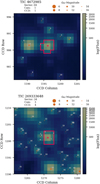 |
Fig. 1 TESS full-frame image of TIC 4672985, from sector 4 (upper panel) and of TOI-2529 in sector 34 (lower panel). Nearby sources detected by Gaia are also shown. The red box corresponds to the aperture used for the photometry extraction. |
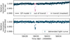 |
Fig. 2 Upper panel: TESS extracted light curve of TIC 4672985 observed in sector 4. The GP model used to correct for the long-term variability is overplotted (solid black line). Lower panel: detrended TESS light curve. |
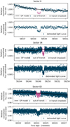 |
Fig. 3 Same as Fig. 2 but for TOI-2529 in sectors 8, 34 and 63 (upper, middle, and lower panel, respectively). |
3.1 Callisto
Callisto is one of the six identical robotic one-meter telescopes of the Search for habitable Planets EClipsing ULtra-cOO1 Stars (SPECULOOS; Delrez et al. 2018) network. Four of them, including Callisto, are installed at the Paranal observatory in Chile. The main scientific goal of SPECULOOS is the detection of transiting terrestrial planets in orbit around nearby (<40 pc) late-type M and L-dwarfs. Each SPECULOOS telescope is equipped with a 2k × 2k CCD, with a field of view of 12′ × 12′ and a pixel scale of 0.35 arcsec pix−1. We observed a transit egress of TIC 4672985 b with Callisto on 2021 September 8, using the ɀ filter and with a cadence of 40 s. The extracted normalized photometry is presented in Fig. 4.
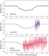 |
Fig. 4 Normalized photometric observations of TIC 4672985 during the transit. The data were obtained in TESS sector 4 (upper panel) and from ground-based telescopes (CALLISTO and OM-ES; middle and lower panels, respectively). The solid lines correspond to the transit models. |
3.2 OM-ES
The Observatoire Moana – E1 Sauce (OM-ES) facility is an equatorial robotic telescope with a 60 cm aperture, located at E1 Sauce Observatory, in Chile. OM-ES is equipped with a 2k × 2k detector, with a pixel scale of of 0.7 arcsec pix−1, and has a standard set of Sloan filters u′, g′, r′, i′. Using this telescope, we observed a partial transit of TIC 4672985 in the night of 2021 November 16. For these observations, we used the i′ filter, and we obtained an image every 49 s. The data reduction and photometry extraction was performed with a set of automated routines that were used previously in other facilities (e.g., Brahm et al. 2020). The extracted normalized photometric data are presented in Fig. 4.
4 Speckle imaging
To search for potential sources of blending or flux contamination, we observed TIC 4672985 with the NN-Explore Exoplanet Stellar Speckle Imager (NESSI; Scott et al. 2018) on the WIYN 3.5 m telescope at Kitt Peak National Observatory, on 2019 October 12. We obtained one-minute sequences of short diffraction-limited exposures in each of the 832 and 562 nm filters with the red and blue NESSI cameras, respectively. The reconstructed speckle images were created following the procedures described in Howell et al. (2011). As we show in Fig. 5, the computed 5σ contrast limits rule out companions brighter than ∆m562 = 3.9 and ∆m832 = 4.4 at separations greater than 0.5 arcsec and ∆m632 = 4.2 and ∆m832 = 4.9 outside of 1 arcsec.
Similarly, we searched for stellar companions to TOI-2529 with speckle imaging on the 4.1 m Southern Astrophysical Research (SOAR) telescope (Tokovinin 2018). To do this, we observed this star with the HRCam on 2021 October 1, in the Cousins I band. This observation was sensitive to a star that is fainter by 5.2 mag at an angular distance of 1 arcsec from the target. More details of the observations within the SOAR TESS survey are available in Ziegler et al. (2020). The 5σ detection sensitivity and speckle autocorrelation functions from the observations are shown in Fig. 6. No nearby stars were detected within 3 arcsec of TOI-2529 in the SOAR observations.
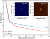 |
Fig. 5 Reconstructed NESSI speckle images for TIC 4672985. The observations were obtained simultaneously at 532 and 832 nm with the blue and red camera (upper left and right images). The corresponding 5σ contrast curves are overplotted (solid red and blue lines, respectively). |
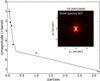 |
Fig. 6 Speckle autocorrelation function obtained in the I band at the SOAR telescope, for TOI-2529. The black dots correspond to the 5σ contrast curve. The solid line corresponds to the linear fit of the data at separations smaller and larger than ~0.2 arcsec. |
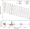 |
Fig. 7 RV curve of TIC4672985. The best Keplerian fit and the observed RV trend are overplotted. |
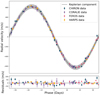 |
Fig. 8 Phase-folded RV curve for TIC 4672985, after subtracting the quadratic trend. The gray region corresponds to 1σ uncertainty in the best-fit model. |
5 Ground-based spectroscopic follow-up
We performed a spectroscopic follow-up of these two stars, using four different high-resolution spectrographs. From the observed spectra, we computed precision radial velocities (RVs), which were used to confirm the planetary nature of the observed photometric transits and to measure their the masses. Similarly, from the cross-correlation function (CCF), we also measured the line bisectors (BVS; Toner & Gray 1988). The resulting RVs and BVS values, with their corresponding 1σ uncertainties are listed in Tables A.1 and A.2, and are also presented in Figs. 7–10.
5.1 CHIRON
We observed TIC4672985 and TOI-2529 with CHIRON (Tokovinin et al. 2013), as part of a large program in the context of the WINE collaboration. CHIRON is a high-resolution fiber-fed spectrograph mounted on the 1.5 m telescope at the Cerro Tololo Inter-american Observatory (CTIO) in Chile. We obtained a total of 24 spectroscopic epochs for TIC 4672985 and 21 epochs for TOI-2529. We adopted exposures times of 1800 s for the two stars, and we used the image-slicer mode, which delivers a spectral resolution of R ~ 80000. The typical signal-to-noise-ratio (S/N) per extracted pixel was ~ 10–20 in the two cases, with corresponding mean RV uncertainties at the ~ 13–15 m s−1 level. The data were reduced using the CHIRON pipeline (Paredes et al. 2021) and the RVs were computed with the pipeline described in Jones et al. (2019).
5.2 FEROS
We collected a total of 20 individual spectra of TIC 4672985, between 2020 December 5 and 2022 January 8, with the Fiber-fed Extended Range Optical Spectrograph (FEROS; Kaufer et al. 1999) high-resolution spectrograph (R ~ 48 000), installed at the 2.2 m telescope, at La Silla. The exposure times were between 900 and 1800 s. FEROS is equipped with two fibers, allowing for either sky-background subtraction or simultaneous wavelength calibration. The latter is the observing mode we used in our observations. Similarly, we observed TOI-2529 a total of 17 times with FEROS between 2020 December 4 and 2021 December 30. For this star the exposure times were between 600 and 900 s. The data were reduced with the CERES pipeline (Brahm et al. 2017a), which also automatically computes the stellar RV and BVS values. The typical uncertainty in the derived FEROS RVs is ~7–8 m s−1 for the two stars.
5.3 HARPS
The High Accuracy Radial velocity Planet Searcher (HARPS; Mayor et al. 2003) is a fibre-fed by the Cassegrain focus of the 3.6m telescope at La Silla Observatory. Using this instrument, we obtained 27 spectra for TOI-2529 and 18 for TIC 4672985. We selected the high-resolution mode (1 arcsec fibre, leads to R ~ 115 000) and the simultaneous wavelength calibration for our observations. The exposure time was 900 s for TIC 4672985 and between 600 s and 900 s for TOI-2529. As for FEROS, the data reduction and RV computation was made with CERES. The mean RV uncertainty is ~6 and 8 m s−1, for TIC 4672985 and TOI-2529, respectively.
5.4 CORALIE
We collected a total of 29 spectra of TIC 4672985 using CORALIE (Queloz et al. 2000), which is mounted on the 1.2 m Leonhard Euler Telescope at La Silla observatory. CORALIE is an echelle high-resolution spectrograph that delivers a resolving power of R ~ 60 000. This instrument is also equipped with two optical fibres, the second of which is fed by either a sky or a simultaneous calibration source, in this case, a Fabry-Perot interferometer. As for FEROS and HARPS, we used the latter configuration to correct for the night drift. The data reduction and RV computation was performed with the CORALIE data reduction software.
6 Stellar parameters
We derived the stellar properties of the two host stars, using the zonal atmospheric stellar parameters estimator (ZASPE; Brahm et al. 2017b) code, following an iterative procedure described in detail elsewhere (e.g., Brahm et al. 2019; Hobson et al. 2021). Briefly, we first coadded the FEROS spectra to create a high S/N observed template of each star. We then used ZASPE to compare the resulting template with a grid of synthetic spectra from the ATLAS9 models (Castelli & Kurucz 2003). After exploring a wide parameter range, we derived a first set of stellar atmospheric parameters (Teff, log 𝑔, [Fe/H] and υ sin i). Then, the physical stellar parameters (M★, R★, L★, ρ★) and the stellar age and visual extinction in the line of sight (Av) were obtained by comparing the stellar broadband photometry, which was converted into absolute magnitude using the Gaia DR2 (Gaia Collaboration 2018) parallaxes, with the synthetic magnitudes from the PARSEC stellar evolutionary models (Bressan et al. 2012). In this process we fixed the metallicity found in the first step and used the initial Teff as a prior for this second step. We repeated this procedure in an iterative way until convergence was reached. The resulting atmospheric and physical parameters for the two stars are listed in Table 1. We note that for the rest of the paper, we adopt the ZASPE stellar parameters. For comparison, we also computed atmospheric and physical parameters for the two stars using the SPECIES code (Soto et al. 2021). They are also listed in Table 1. In general, the two methods agree very well. We note that the uncertainties listed in Table 1 correspond to the internal uncertainties obtained by the different methods we used, and they do not consider systematic errors. However, following Tayar et al. (2022), we add systematic uncertainties of 2% in quadrature to the stellar luminosity, an uncertainty of 4% to the stellar radius, an uncertainty of 5% to the stellar mass, and an uncertainty of 20% to the stellar age in the following sections. This significantly affects the final planet parameters and their corresponding uncertainties.
Finally, we performed a periodogram analysis of the V-band all sky automated survey (ASAS; Pojmanski 1997) and the all-sky automated survey for supernovae (ASAS-SN; Kochanek et al. 2017) photometric data of these two stars to estimate the stellar age via gyrochronology. No significant periodicity was found in the periodogram of either star (see Figs. A.3 and A.4), and their rotational period could therefore not be derived.
Stellar parameters.
7 Joint photometric and radial velocity analysis
We jointly modeled the ground- and space-based photometry with the derived RVs for the two systems presented here. To do this we used juliet (Espinoza et al. 2019), a python-based package that employs Bayesian inference and nested sampling to achieve model fitting and comparison. juliet uses the radvel package (Fulton et al. 2018) for the RV data modeling, and batman (Kreidberg 2015) for the photometric transit model. In addition, we used the dynesty package (Speagle 2020), which is incorporated in juliet, to sample the posterior distributions. We used uniform priors for the orbital and transit parameters. Based on the effective temperature of both host stars and following (Espinoza & Jordán 2016), we adopted a logarithmic limb-darkening law for both ground- and space-based photometry, also setting uniform priors on the q1 and q2 parameters (see Kipping 2013). In the case of TIC 4672985, we fixed the dilution factor to 1, while in the case of TOI-2529, we fit this parameter by adopting a uniform prior based on the expected level of contamination by nearby sources (see Sect. 2). Following the approach presented in Espinoza et al. (2019), we used the estimated stellar density to constrain a/R*, this time using a normal distribution prior, with µ and σ derived using ZASPE. Finally, we adopted uniform priors for the RV zeropoint and extra jitter, while for the photometric extra jitter, we used log-uniform priors. We note that for TIC 4672985, we also modeled the RV trend with a linear and quadratic trend. The resulting Bayesian evidence favored the quadratic model (∆ log ɀ = 6.1). The prior and resulting posterior distributions of the pertinent parameters for TIC 4672985 b and TOI-2529 b are presented in Tables 2 and 3, respectively2. Similarly, the transit models for TIC 4672985 b and TOI-2529 b are presented in Figs. 4 and 11, respectively. Finally, for these two systems, no significant periodic signal is detected in the RV residuals (see Figs. A.1 and A.2).
8 Discussion
8.1 TOI-2529 b and TIC 4672985b in the context of transiting giant planets
Figure 12 shows the mass-radius distribution of known3 transiting giant planets, with a mass and radius determination better than 20%, including the position of TOI-2529 b and TIC 4672985 b. For comparison, a solar metallicity, 1 Gyr old ATMO2020 isochrone (Phillips et al. 2020) is overplotted. The deuterium-burning limit (~11–16 MJ; Spiegel et al. 2011) is also shown. TOI-2529 b is a new example of a growing population of well-characterized transiting giant planets with orbital periods > 10 days. Because this type of planets has a mild insolation level, they cool down slowly while losing their internal energy in the form of radiation. As a result, and after ~1 Gyr from their birth, they shrink to ~1 RJ and reach an effective temperature between ~200–500 K. In contrast, closer-in gas giants remain significantly hotter and therefore have larger radii at a given age. These two different populations can be clearly distinguished in Fig. 12, where hot Jupiters show a radius distribution between ~1–2 RJ, while most warm giant planets pile up around ~1 RJ. On the other hand, TIC 4672985 b is a unique example of a transiting warm planet that is in the transition between the super-Jupiter and the BD regime. Figure 12 shows that this object stands alone in the deuterium-burning limit region among the population of warm transiting giant planets.
Similarly, Fig. 13 shows the bulk density as a function of the planet mass. Again, there is a clear distinction between the hot and warm giant planets. Hot giants present a large scatter, with many examples of extremely low-density objects, as opposed to the warmer counterpart, which mainly follows a linear correlation between these two quantities in log-log space, as predicted by evolutionary models.
Finally, Fig. 14 shows the eccentricity distribution as a function of the orbital separation. We included only planets with a mass determination4 better than 20% and an eccentricity uncertainty of σe < 0.15. While TOI 2529 b presents a low-eccentricity level, which is common among the population of low-mass giant planets orbiting beyond ~ 0.1 AU, TIC 4672985 b stands out as a unique massive warm substellar companion in a nearly circular orbit.
TIC 4672985 model parameters.
TOI-2529 model parameters.
8.2 Internal composition of the planets
To study the composition of the planets presented here, we compared their radii with planet evolutionary models. In particular, we used the modules for experiments in stellar astrophysics (MESA; Paxton et al. 2011), and we generated different giant planet models, with a different envelope composition and core mass, and we also included the effect of the stellar irradiation. To do this, we used the updated5 version of the ρ-T OPAL tables (Rogers & Nayfonov 2002), with the extension to lower temperatures and densities from the SCvH equation of state (EOS) presented in Saumon et al. (1995). We note that we mimicked the presence of metals in the H/He SCvH EOS by setting an equivalent He content given by Y′ = Y + Z, as shown in Chabrier & Baraffe (1997). Similarly, we employed the low-temperature opacity tables from Ferguson et al. (2005) and Freedman et al. (2008), coupled with the heavy element distribution of Grevesse & Sauval (1998). These tables also include the radiative opacities from molecules and grains. Finally, we adopted the solar metallicity Z = 0.0152 with the corresponding helium-scaled mass fraction: Y = 0.2485 + 1.78 Z, derived in Bressan et al. (2012), which is the one used by ZASPE (see Sect. 6).
We first created an adiabatically contracting model using the create_initial_model routine (Paxton et al. 2013), which builds a planetary model with a given initial radius and gas mass.
In our calculations, we set the initial radius to 5 RJ for all the different models, with the possibility of including an inert rocky core with constant density. Finally, we evolved the different models for 8 Gyr, and also included the planet insolation. To do this, we implemented the gray_irradiated option inside the atm module, which uses the angle-averaged temperature profile described in Guillot (2010). This option includes both the stellar irradiation and the cooling flux from the planetary interior. Instead of using the current insolation value, we computed the incident flux received by the planet, by fixing the orbital distance to its current value, and we updated the host star luminosity in steps of 1 Gyr, using PARSEC stellar evolutionary models that matched the stellar parameters for each star, as derived here (see Table 1). This is particularly important for TOI-2529, which is in the subgiant phase, and therefore, its luminosity has increased significantly since the zero-age main sequence.
To study the composition of TOI-2529 b, we computed different models with a total mass of 2.34 MJ. In our calculations, we included a coreless and a rocky core model with a different amount of metals in the H/He gas envelope (Zenv). Finally, we assumed that the age of the planet is the same as that of the host star, considering the very short lifetime of protoplanetary disks (e.g., Mamajek 2009). Figure 15 shows the position of TOI-2529 b in the age-radius diagram. Two different models with a 40 M⊕ core with constant density of 20 [gr cm−3] and with different envelope compositions are overplotted. For comparison, a model with incident flux (inc) equal to zero is also shown. A possible model that reproduces the current radius of the planet well is the model with a rocky core, Zenv = 0.019 (the same as the host star) and with stellar irradiation. However, we note that different combinations of the core composition and Zenv can reproduce observed properties of the planet within the observational uncertainties in age and radius. By fixing the Zenv to 0.019 and the density of the core to 20 [gr cm−3], we found that core masses up to ~ 100 M⊕ match the observed age-radius of the planet within 1σ. This corresponds to a heavy element enrichment of Zp/Z★ ~ 1–8. We also note that even though TOI-2529 b is a WJ, the effect of the stellar irradiation plays an important role in its cooling evolution, and thus in its radius as a function of time. After ~ 1 Gyr, the effect of the delayed cooling due to the incident flux clearly leads to a radius tthat is ~4% larger than in the model without incident flux (blue line in Fig. 15). Moreover, heat deposition from the stellar flux in the planet interior (e.g. Ginzburg & Sari 2016), would further slow the planet cooling rate down, and thus models with larger heavy element fraction would fit the observed radius of the planet better. Finally, and for comparison, a simple model of Jupiter (age = 4.6 Gyr) is overplotted (green line).
Similarly, Fig. 16 shows the position of TIC 4672985 b in the age-radius diagram. Again, different models with different compositions, and including the stellar irradiation are shown. For comparison, we also included a model with finc = 0. We note that for this object we did not include a rocky core and we neglected the additional heating from deuterium burning, which can increase the luminosity and halt its contraction at early epochs (≲50–100 Myr; e.g. Chabrier et al. 2000; Paxton et al. 2011; Mollière & Mordasini 2012), but it has a negligible effect in the long-term evolution of the planet. Although a model with the same composition as of the host star matches the current position of TIC 4672985 b at the 1σ level, models with subsolar metallicity are clearly preferred. This means that no heavy-elements enrichment with respect to the parent star need be invoked.
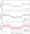 |
Fig. 11 Normalized TESS photometry of TOI-2529 around the transit in sectors 8, 34, and 63 (upper, middle, and lower panels, respectively). The 30-min binned data and the best-fit transit model are overplotted. |
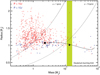 |
Fig. 12 Mass-radius distribution of known transiting giant planets as of June 30, 2023. The open red circles and blue dots correspond to orbital periods shorter and longer than 10 days, respectively. The positions of TIC 4672985 b (black diamond) and TOI-2529 b (black square) are also shown. The shaded area represents the theoretical deuterium-burning limit. The solid line corresponds to a 1 Gyr old and solar metallicity ATMO2020 isochrone. Two isodensity curves for 1 and 10 [gr cm−3] are also plotted (dashed left and right lines, respectively). |
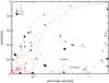 |
Fig. 14 Eccentricity distribution as a function of the orbital distance for known giant planets with eccentricity precision of σe < 0.15 and mass precision better than 20%, including TIC 4672985 b and TOI-2529 b. The size of the symbols is proportional to the square of the planet’s mass. For more clarity, we split the data into two populations, with masses below and above 5 MJ (red and black dots, respectively). The dotted lines correspond to high-eccentricity migration pathways at constant angular momentum (e.g. Dong et al. 2021), with final orbital distance of 0.05 and 0.10 AU (left and right curves, respectively). |
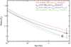 |
Fig. 15 Position of TOI-2529 b in the age-radius diagram (black dot). Planet evolutionary models with different envelope composition and insolation level over-plotted. For comparison, a simple model of Jupiter is also shown. |
9 Summary and conclusions
We used space- and ground-based photometry from different facilities, combined with precision RVs obtained from spectroscopic data collected with different instruments, to characterize two transiting giant planets orbiting the subgiant star TOI-2529 and the main-sequence star TIC 4672985. From the joint analysis we derived the following parameters for  and
and  . With an equilibrium temperature of ~636 K due to a relatively low current insolation of 3.7 × 10⁷ [erg s−1 cm−2], this planet is an excellent example of an emerging population of very well characterized transiting WJs. In terms of the orbital configuration, TOI-2529 b is found in a nearly circular orbit, which is consistent with an in situ formation channel via core-accretion (e.g., Bodenheimer et al. 2000; Boley et al. 2016; Batygin et al. 2016) or by a type II disk migration pathway (e.g. Lin & Papaloizou 1993). In this scenario, even in the case of a Jupiter-mass planet in a highly inclined and eccentric orbit (e.g., due to planet-planet interactions; Weidenschilling & Marzari 1996), the tidal interactions with the disk lead to a rapid damping (on timescales of about 103 yr) of the inclination and the eccentricity (Marzari & Nelson 2009). In addition, TOI-2529 b orbits a metal-rich star, following the well-known planet-metallicity correlation for gas giants orbiting FGK dwarf stars (Gonzalez 1997; Santos et al. 2004; Fischer & Valenti 2005; Adibekyan 2019; Osborn & Bayliss 2020), which is also valid for more massive evolved stars (e.g., Jones et al. 2016). This correlation provides strong observational support for the core-accretion formation model. Furthermore, based on our calculations, the planet composition is consistent with a rocky core and heavy element enrichment with respect to its parent star, providing further evidence of a formation channel via core accretion. Given its low equilibrium temperature and relatively compact radius, TOI-2529 b has a very low transmission spectroscopy metric (TSM; Kempton et al. 2018) of ~5, making this a very challenging system for a detailed atmospheric characterization study. On the other hand, we estimated a Rossiter-McLaughlin (R-M; Rossiter 1924; McLaughlin 1924) RV amplitude of ~7 m s−1 (assuming i★ = 90 deg; see Eq. (1) in Triaud 2018), which is within the reach of stable instruments mounted on 8-meter-class telescopes (due to the relatively faintness of the target), such as ESPRESSO (Pepe et al. 2021). A low obliquity level would provide further observational support for the disk migration scenario (e.g. Lin et al. 1996), highlighting the importance of a future R-M characterization of this system.
For TIC 4672985 b we obtained the following orbital parameters:  , and
, and  . Additionally, we detected an RV trend at the ~350 m s−1 yr−1 level, indicating the presence of either an outer BD companion in the system or a bound low-luminosity stellar companion. Thus, this is a unique system. It is the first warm transiting substellar companion that is located in the regime of super-Jupiters to brown dwarfs and has a precise mass and radius determination. Interestingly, TIC 4672985 b also presents a very low eccentricity, which is extremely rare among planets of its class. Moreover, this observational result challenges theoretical migration models, where unlike the case of lower-mass gas giants, a low eccentricity like this is not a direct indication of coplanar migration via disk interactions because even at low inclinations with respect to the disk, the eccentricity can be excited by this mechanism in this planetary mass regime (Bitsch et al. 2013; Dunhill et al. 2013). Similarly, the presence of an outer companion might induce eccentricity growth via Kozai-Lidov cycles (Kozai 1962; Lidov 1962) or through nearly coplanar apsidal precession resonances (e.g., Anderson & Lai 2017). Measuring the obliquity level for this object (predicted R-M amplitude of ~8 m s−1) is thus mandatory to further characterize the orbital configuration of the system. On the other hand, and due to its very low TSM of ~1, it is not possible to perform a detailed atmospheric study of this planet.
Finally, from our calculations, the position of TIC 4672985 b in the age-radius diagram is consistent with a coreless model with subsolar metallicity, meaning that no metal enhancement with respect to the parent star is present. This could be an indication that this object was formed by gravitational instability (e.g., Boss 1997; Bate 2012), as was shown to be the case for substellar objects more massive than ~10 MJ (Schlaufman 2018).
Acknowledgements
The results reported herein benefited from collaborations and/or information exchange within NASA’s Nexus for Exoplanet System Science (NExSS) research coordination network sponsored by NASA’s Science Mission Directorate under Agreement No. 80NSSC21K0593 for the program “Alien Earths”. We thank the Swiss National Science Foundation (SNSF) and the Geneva University for their continuous support to the planet search programs. This work has been in particular carried out in the frame of the National Centre for Competence in Research PlanetS supported by the SNSF under grants 51NF40_182901 and 51NF40_205606 This publication made use of The Data & Analysis Center for Exoplanets (DACE), which is a facility based at the University of Geneva dedicated to extrasolar planets data visualisation, exchange and analysis. DACE is a platform of NCCR PlanetS and is available at https://dace.unige.ch. This paper made use of data collected by the TESS mission and are publicly available from the Mikulski Archive for Space Telescopes (MAST) operated by the Space Telescope Science Institute (STScI). Funding for the TESS mission is provided by NASA’s Science Mission Directorate. We acknowledge the use of public TESS data from pipelines at the TESS Science Office and at the TESS Science Processing Operations Center. Resources supporting this work were provided by the NASA High-End Computing (HEC) Program through the NASA Advanced Supercomputing (NAS) Division at Ames Research Center for the production of the SPOC data products. This paper is based on data collected by the SPECULOOS-South Observatory at the ESO Paranal Observatory in Chile. The ULiege s contribution to SPECULOOS has received funding from the European Research Council under the European Union’s Seventh Framework Programme (FP/2007-2013) (grant Agreement nº 336480/SPECULOOS), from the Balzan Prize and Francqui Foundations, from the Belgian Scientific Research Foundation (F.R.S.-FNRS; grant n° T.0109.20), from the University of Liege, and from the ARC grant for Concerted Research Actions financed by the Wallonia-Brussels Federation. The Cambridge contribution is supported by a grant from the Simons Foundation (PI Queloz, grant number 327127). The Birmingham contribution to SPECULOOS is in part funded by the European Union s Horizon 2020 research and innovation programme (grant’s agreement n° 803193/BEBOP), from the MERAC foundation, and from the Science and Technology Facilities Council (STFC; grant n° ST/S00193X/1, and ST/W000385/1). This publication benefits from the support of the French Community of Belgium in the context of the FRIA Doctoral Grant awarded to MT. M.L. acknowledges support of the Swiss National Science Foundation under grant number PCEFP2_194576. M.R.S. acknowledges support from the UK Science and Technology Facilities Council (ST/T000295/1) and support from the European Space Agency as an ESA Research Fellow. M.T.P. acknowledges the support of the Fondecyt-ANID Post-doctoral fellowship No. 3210253. T.T. acknowledges support by the DFG Research Unit FOR 2544 “Blue Planets around Red Stars” project No. KU 3625/2-1. T.T. further acknowledges support by the BNSF program “VIHREN-2021” project No. KP-06-DV/5. D.D. acknowledges support from the NASA Exoplanet Research Program grant 18-2XRP18_2-0136, and from the TESS Guest Investigator Program grants 80NSSC22K0185 and 80NSSC23K0769. J.C. acknowledges support of the South Carolina Space Grant Consortium. R.B. acknowledges support from FONDECYT project 11200751 and from project IC120009 “Millennium Institute of Astrophysics (MAS)” of the Millenium Science Initiative. M.U. gratefully acknowledges funding from the Research Foundation Flanders (FWO) by means of a junior postdoctoral fellowship (grant agreement No. 1247624N).
Appendix A Radial velocity tables
Relative radial velocities for TIC 4672985.
Relative radial velocities for TOI-2529.
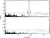 |
Fig. A.1 Upper panel: Periodogram of the combined RVs of TIC 4672985, after correcting by the long-term quadratic trend and applying the differential instrumental zero points. The dashed horizontal lines correspond to 10%, 1% and 0.1% false-alarm probability (from bottom to top). The period of maximum power is labeled. Lower panel: Periodogram of the post-fit residuals. |
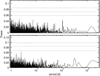 |
Fig. A.3 Periodogram of the ASAS and ASAS-SN V-band photometry of TIC 4672985 (upper and lower panel, respectively). The dashed horizontal lines correspond to 10%, 1% and 0.1% false-alarm probability (from bottom to top). |
References
- Adibekyan, V. 2019, Geosciences, 9, 105 [Google Scholar]
- Albrecht, S. H., Dawson, R. I., & Winn, J. N. 2022, PASP, 134, 082001 [NASA ADS] [CrossRef] [Google Scholar]
- Anderson, K. R., & Lai, D. 2017, MNRAS, 472, 3692 [NASA ADS] [CrossRef] [Google Scholar]
- Baraffe, I., Chabrier, G., & Barman, T. 2010, Rep. Prog. Phys., 73, 016901 [NASA ADS] [CrossRef] [Google Scholar]
- Bate, M. R. 2012, MNRAS, 419, 3115 [NASA ADS] [CrossRef] [Google Scholar]
- Batygin, K., & Stevenson, D. J. 2010, ApJ, 714, L238 [NASA ADS] [CrossRef] [Google Scholar]
- Batygin, K., Bodenheimer, P. H., & Laughlin, G. P. 2016, ApJ, 829, 114 [Google Scholar]
- Beaugé, C., & Nesvorný, D. 2012, ApJ, 751, 119 [CrossRef] [Google Scholar]
- Bitsch, B., Crida, A., Libert, A. S., & Lega, E. 2013, A&A, 555, A124 [NASA ADS] [CrossRef] [EDP Sciences] [Google Scholar]
- Bodenheimer, P., Hubickyj, O., & Lissauer, J. J. 2000, Icarus, 143, 2 [Google Scholar]
- Bodenheimer, P., Lin, D. N. C., & Mardling, R. A. 2001, ApJ, 548, 466 [NASA ADS] [CrossRef] [Google Scholar]
- Boley, A. C., Granados Contreras, A. P., & Gladman, B. 2016, ApJ, 817, L17 [Google Scholar]
- Boss, A. P. 1997, Science, 276, 1836 [Google Scholar]
- Brahm, R., Jordán, A., & Espinoza, N. 2017a, PASP, 129, 034002 [NASA ADS] [CrossRef] [Google Scholar]
- Brahm, R., Jordán, A., Hartman, J., & Bakos, G. 2017b, MNRAS, 467, 971 [NASA ADS] [Google Scholar]
- Brahm, R., Espinoza, N., Jordán, A., et al. 2019, AJ, 158, 45 [Google Scholar]
- Brahm, R., Nielsen, L. D., Wittenmyer, R. A., et al. 2020, AJ, 160, 235 [Google Scholar]
- Brahm, R., Ulmer-Moll, S., Hobson, M. J., et al. 2023, AJ, 165, 227 [NASA ADS] [CrossRef] [Google Scholar]
- Bressan, A., Marigo, P., Girardi, L., et al. 2012, MNRAS, 427, 127 [NASA ADS] [CrossRef] [Google Scholar]
- Carmichael, T. W., Quinn, S. N., Zhou, G., et al. 2021, AJ, 161, 97 [Google Scholar]
- Castelli, F., & Kurucz, R. L. 2003, IAU Symp., 210, A20 [Google Scholar]
- Chabrier, G., & Baraffe, I. 1997, A&A, 327, 1039 [NASA ADS] [Google Scholar]
- Chabrier, G., Baraffe, I., Allard, F., & Hauschildt, P. 2000, ApJ, 542, L119 [CrossRef] [Google Scholar]
- Cutri, R. M., Skrutskie, M. F., van Dyk, S., et al. 2003, VizieR Online Data Catalog: II/246 [Google Scholar]
- Delrez, L., Gillon, M., Queloz, D., et al. 2018, SPIE Conf. Ser., 10700, 107001I [Google Scholar]
- Demory, B.-O., & Seager, S. 2011, ApJS, 197, 12 [NASA ADS] [CrossRef] [Google Scholar]
- Dong, J., Huang, C. X., Dawson, R. I., et al. 2021, ApJS, 255, 6 [NASA ADS] [CrossRef] [Google Scholar]
- Dunhill, A. C., Alexander, R. D., & Armitage, P. J. 2013, MNRAS, 428, 3072 [NASA ADS] [CrossRef] [Google Scholar]
- Espinoza, N., & Jordan, A. 2016, MNRAS, 457, 3573 [NASA ADS] [CrossRef] [Google Scholar]
- Espinoza, N., Kossakowski, D., & Brahm, R. 2019, MNRAS, 490, 2262 [Google Scholar]
- Ferguson, J. W., Alexander, D. R., Allard, F., et al. 2005, ApJ, 623, 585 [Google Scholar]
- Fischer, D. A., & Valenti, J. 2005, ApJ, 622, 1102 [NASA ADS] [CrossRef] [Google Scholar]
- Foreman-Mackey, D., Agol, E., Ambikasaran, S., & Angus, R. 2017, AJ, 154, 220 [Google Scholar]
- Fortney, J. J., Marley, M. S., & Barnes, J. W. 2007, ApJ, 659, 1661 [Google Scholar]
- Freedman, R. S., Marley, M. S., & Lodders, K. 2008, ApJS, 174, 504 [NASA ADS] [CrossRef] [Google Scholar]
- Fulton, B. J., Petigura, E. A., Blunt, S., & Sinukoff, E. 2018, PASP, 130, 044504 [Google Scholar]
- Gaia Collaboration. 2020, VizieR Online Data Catalog: I/350 [Google Scholar]
- Gaia Collaboration, (Brown, A. G. A., et al.) 2018, A&A, 616, A1 [NASA ADS] [CrossRef] [EDP Sciences] [Google Scholar]
- Gaia Collaboration (Vallenari, A., et al.) 2023, A&A, 674, A1 [NASA ADS] [CrossRef] [EDP Sciences] [Google Scholar]
- Ginzburg, S., & Sari, R. 2016, ApJ, 819, 116 [NASA ADS] [CrossRef] [Google Scholar]
- Gonzalez, G. 1997, MNRAS, 285, 403 [Google Scholar]
- Grevesse, N., & Sauval, A. J. 1998, Space Sci. Rev., 85, 161 [Google Scholar]
- Grunblatt, S. K., Huber, D., Gaidos, E., et al. 2017, AJ, 154, 254 [Google Scholar]
- Guillot, T. 2010, A&A, 520, A27 [NASA ADS] [CrossRef] [EDP Sciences] [Google Scholar]
- Guillot, T., Burrows, A., Hubbard, W. B., Lunine, J. I., & Saumon, D. 1996, ApJ, 459, L35 [Google Scholar]
- Hobson, M. J., Brahm, R., Jordán, A., et al. 2021, AJ, 161, 235 [NASA ADS] [CrossRef] [Google Scholar]
- Høg, E., Fabricius, C., Makarov, V. V., et al. 2000, A&A, 355, L27 [Google Scholar]
- Howell, S. B., Everett, M. E., Sherry, W., Horch, E., & Ciardi, D. R. 2011, AJ, 142, 19 [Google Scholar]
- Jackson, B., Greenberg, R., & Barnes, R. 2008, ApJ, 681, 1631 [NASA ADS] [CrossRef] [Google Scholar]
- Jenkins, J. M., Twicken, J. D., McCauliff, S., et al. 2016, Proc. SPIE, 9913, 99133E [Google Scholar]
- Jones, M. I., Jenkins, J. S., Brahm, R., et al. 2016, A&A, 590, A38 [NASA ADS] [CrossRef] [EDP Sciences] [Google Scholar]
- Jones, M. I., Brahm, R., Espinoza, N., et al. 2019, A&A, 625, A16 [NASA ADS] [CrossRef] [EDP Sciences] [Google Scholar]
- Kaltenegger, L., & Sasselov, D. 2011, ApJ, 736, L25 [Google Scholar]
- Kaufer, A., Stahl, O., Tubbesing, S., et al. 1999, The Messenger, 95, 8 [Google Scholar]
- Kempton, E. M. R., Bean, J. L., Louie, D. R., et al. 2018, PASP, 130, 114401 [Google Scholar]
- Kipping, D. M. 2013, MNRAS, 435, 2152 [Google Scholar]
- Knierim, H., Shibata, S., & Helled, R. 2022, A&A, 665, L5 [NASA ADS] [CrossRef] [EDP Sciences] [Google Scholar]
- Kochanek, C. S., Shappee, B. J., Stanek, K. Z., et al. 2017, PASP, 129, 104502 [Google Scholar]
- Komacek, T. D., Thorngren, D. P., Lopez, E. D., & Ginzburg, S. 2020, ApJ, 893, 36 [NASA ADS] [CrossRef] [Google Scholar]
- Kozai, Y. 1962, AJ, 67, 591 [Google Scholar]
- Kreidberg, L. 2015, PASP, 127, 1161 [Google Scholar]
- Laughlin, G., Crismani, M., & Adams, F. C. 2011, ApJ, 729, L7 [NASA ADS] [CrossRef] [Google Scholar]
- Lidov, M. L. 1962, Planet. Space Sci., 9, 719 [Google Scholar]
- Lin, D. N. C., Bodenheimer, P., & Richardson, D. C. 1996, Nature, 380, 606 [Google Scholar]
- Lin, D. N. C., & Papaloizou, J. C. B. 1993, in Protostars and Planets III, eds. E. H. Levy, & J. I. Lunine (Tucson: University of Arizona Press), 749 [Google Scholar]
- Mamajek, E. E. 2009, AIP Conf. Ser., 1158, 3 [Google Scholar]
- Marzari, F., & Nelson, A. F. 2009, ApJ, 705, 1575 [NASA ADS] [CrossRef] [Google Scholar]
- Mayor, M., Pepe, F., Queloz, D., et al. 2003, The Messenger, 114, 20 [NASA ADS] [Google Scholar]
- McLaughlin, D. B. 1924, ApJ, 60, 22 [Google Scholar]
- Mollière, P., & Mordasini, C. 2012, A&A, 547, A105 [NASA ADS] [CrossRef] [EDP Sciences] [Google Scholar]
- Munari, U., Henden, A., Frigo, A., et al. 2014, AJ, 148, 81 [NASA ADS] [CrossRef] [Google Scholar]
- Osborn, A., & Bayliss, D. 2020, MNRAS, 491, 4481 [Google Scholar]
- Paredes, L. A., Henry, T. J., Quinn, S. N., et al. 2021, AJ, 162, 176 [NASA ADS] [CrossRef] [Google Scholar]
- Paxton, B., Bildsten, L., Dotter, A., et al. 2011, ApJS, 192, 3 [Google Scholar]
- Paxton, B., Cantiello, M., Arras, P., et al. 2013, ApJS, 208, 4 [Google Scholar]
- Pepe, F., Cristiani, S., Rebolo, R., et al. 2021, A&A, 645, A96 [NASA ADS] [CrossRef] [EDP Sciences] [Google Scholar]
- Petrovich, C., & Tremaine, S. 2016, ApJ, 829, 132 [NASA ADS] [CrossRef] [Google Scholar]
- Phillips, M. W., Tremblin, P., Baraffe, I., et al. 2020, A&A, 637, A38 [NASA ADS] [CrossRef] [EDP Sciences] [Google Scholar]
- Pojmanski, G. 1997, Acta Astron., 47, 467 [Google Scholar]
- Queloz, D., Mayor, M., Naef, D., et al. 2000, in From Extrasolar Planets to Cosmology: The VLT Opening Symposium, eds. J. Bergeron, & A. Renzini (Berlin: Springer), 548 [Google Scholar]
- Rasio, F. A., & Ford, E. B. 1996, Science, 274, 954 [Google Scholar]
- Ricker, G. R., Winn, J. N., Vanderspek, R., et al. 2015, J. Astron. Telesc. Instrum. Syst., 1, 014003 [Google Scholar]
- Rogers, F. J., & Nayfonov, A. 2002, ApJ, 576, 1064 [Google Scholar]
- Rossiter, R. A. 1924, ApJ, 60, 15 [Google Scholar]
- Santos, N. C., Israelian, G., & Mayor, M. 2004, A&A, 415, 1153 [NASA ADS] [CrossRef] [EDP Sciences] [Google Scholar]
- Sarkis, P., Mordasini, C., Henning, T., Marleau, G. D., & Mollière, P. 2021, A&A, 645, A79 [NASA ADS] [CrossRef] [EDP Sciences] [Google Scholar]
- Saumon, D., Chabrier, G., & van Horn, H. M. 1995, ApJS, 99, 713 [NASA ADS] [CrossRef] [Google Scholar]
- Schlaufman, K. C. 2018, ApJ, 853, 37 [Google Scholar]
- Scott, N. J., Howell, S. B., Horch, E. P., & Everett, M. E. 2018, PASP, 130, 054502 [Google Scholar]
- Soto, M. G., Jones, M. I., & Jenkins, J. S. 2021, A&A, 647, A157 [NASA ADS] [CrossRef] [EDP Sciences] [Google Scholar]
- Speagle, J. S. 2020, MNRAS, 493, 3132 [Google Scholar]
- Spiegel, D. S., Burrows, A., & Milsom, J. A. 2011, ApJ, 727, 57 [Google Scholar]
- Stassun, K. G., Oelkers, R. J., Paegert, M., et al. 2019, AJ, 158, 138 [Google Scholar]
- Tayar, J., Claytor, Z. R., Huber, D., & van Saders, J. 2022, ApJ, 927, 31 [NASA ADS] [CrossRef] [Google Scholar]
- Thorngren, D. P., & Fortney, J. J. 2018, AJ, 155, 214 [Google Scholar]
- Tokovinin, A. 2018, PASP, 130, 035002 [Google Scholar]
- Tokovinin, A., Fischer, D. A., Bonati, M., et al. 2013, PASP, 125, 1336 [NASA ADS] [CrossRef] [Google Scholar]
- Toner, C. G., & Gray, D. F. 1988, ApJ, 334, 1008 [NASA ADS] [CrossRef] [Google Scholar]
- Triaud, A. H. M. J. 2018, in Handbook of Exoplanets, eds. H. J. Deeg, & J. A. Belmonte (Berlin: Springer), 2 [Google Scholar]
- Ward, W. R. 1997, Icarus, 126, 261 [Google Scholar]
- Weidenschilling, S. J., & Marzari, F. 1996, Nature, 384, 619 [Google Scholar]
- Ziegler, C., Tokovinin, A., Briceño, C., et al. 2020, AJ, 159, 19 [Google Scholar]
For the equilibrium temperature we adopted a zero Bond albedo and β = 1; see Kaltenegger & Sasselov (2011).
Data from NASA Exoplanet Archive, as of June 30, 2023. We complemented this list with known transiting brown-dwarf (BDs) from Carmichael et al. (2021).
We included only transiting planets so as to have actual mass measurements rather than RV values of Mp sin i that only provide lower limits to Mp.
All Tables
All Figures
|
Fig. 1 TESS full-frame image of TIC 4672985, from sector 4 (upper panel) and of TOI-2529 in sector 34 (lower panel). Nearby sources detected by Gaia are also shown. The red box corresponds to the aperture used for the photometry extraction. |
| In the text | |
|
Fig. 2 Upper panel: TESS extracted light curve of TIC 4672985 observed in sector 4. The GP model used to correct for the long-term variability is overplotted (solid black line). Lower panel: detrended TESS light curve. |
| In the text | |
|
Fig. 3 Same as Fig. 2 but for TOI-2529 in sectors 8, 34 and 63 (upper, middle, and lower panel, respectively). |
| In the text | |
|
Fig. 4 Normalized photometric observations of TIC 4672985 during the transit. The data were obtained in TESS sector 4 (upper panel) and from ground-based telescopes (CALLISTO and OM-ES; middle and lower panels, respectively). The solid lines correspond to the transit models. |
| In the text | |
|
Fig. 5 Reconstructed NESSI speckle images for TIC 4672985. The observations were obtained simultaneously at 532 and 832 nm with the blue and red camera (upper left and right images). The corresponding 5σ contrast curves are overplotted (solid red and blue lines, respectively). |
| In the text | |
|
Fig. 6 Speckle autocorrelation function obtained in the I band at the SOAR telescope, for TOI-2529. The black dots correspond to the 5σ contrast curve. The solid line corresponds to the linear fit of the data at separations smaller and larger than ~0.2 arcsec. |
| In the text | |
|
Fig. 7 RV curve of TIC4672985. The best Keplerian fit and the observed RV trend are overplotted. |
| In the text | |
|
Fig. 8 Phase-folded RV curve for TIC 4672985, after subtracting the quadratic trend. The gray region corresponds to 1σ uncertainty in the best-fit model. |
| In the text | |
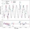 |
Fig. 9 Same as Fig. 7, but for TOI-2529. |
| In the text | |
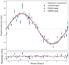 |
Fig. 10 Same as Fig. 8, but for TOI-2529. |
| In the text | |
|
Fig. 11 Normalized TESS photometry of TOI-2529 around the transit in sectors 8, 34, and 63 (upper, middle, and lower panels, respectively). The 30-min binned data and the best-fit transit model are overplotted. |
| In the text | |
|
Fig. 12 Mass-radius distribution of known transiting giant planets as of June 30, 2023. The open red circles and blue dots correspond to orbital periods shorter and longer than 10 days, respectively. The positions of TIC 4672985 b (black diamond) and TOI-2529 b (black square) are also shown. The shaded area represents the theoretical deuterium-burning limit. The solid line corresponds to a 1 Gyr old and solar metallicity ATMO2020 isochrone. Two isodensity curves for 1 and 10 [gr cm−3] are also plotted (dashed left and right lines, respectively). |
| In the text | |
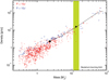 |
Fig. 13 Same as Fig. 12, but for the planet density. |
| In the text | |
|
Fig. 14 Eccentricity distribution as a function of the orbital distance for known giant planets with eccentricity precision of σe < 0.15 and mass precision better than 20%, including TIC 4672985 b and TOI-2529 b. The size of the symbols is proportional to the square of the planet’s mass. For more clarity, we split the data into two populations, with masses below and above 5 MJ (red and black dots, respectively). The dotted lines correspond to high-eccentricity migration pathways at constant angular momentum (e.g. Dong et al. 2021), with final orbital distance of 0.05 and 0.10 AU (left and right curves, respectively). |
| In the text | |
|
Fig. 15 Position of TOI-2529 b in the age-radius diagram (black dot). Planet evolutionary models with different envelope composition and insolation level over-plotted. For comparison, a simple model of Jupiter is also shown. |
| In the text | |
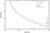 |
Fig. 16 Same as Fig. 15, but for TIC 4672985 b. |
| In the text | |
|
Fig. A.1 Upper panel: Periodogram of the combined RVs of TIC 4672985, after correcting by the long-term quadratic trend and applying the differential instrumental zero points. The dashed horizontal lines correspond to 10%, 1% and 0.1% false-alarm probability (from bottom to top). The period of maximum power is labeled. Lower panel: Periodogram of the post-fit residuals. |
| In the text | |
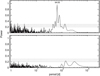 |
Fig. A.2 Same as for Fig. A.1, but for TOI-2529. |
| In the text | |
|
Fig. A.3 Periodogram of the ASAS and ASAS-SN V-band photometry of TIC 4672985 (upper and lower panel, respectively). The dashed horizontal lines correspond to 10%, 1% and 0.1% false-alarm probability (from bottom to top). |
| In the text | |
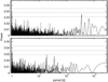 |
Fig. A.4 Same as for Fig. A.3, but for TOI-2529. |
| In the text | |
Current usage metrics show cumulative count of Article Views (full-text article views including HTML views, PDF and ePub downloads, according to the available data) and Abstracts Views on Vision4Press platform.
Data correspond to usage on the plateform after 2015. The current usage metrics is available 48-96 hours after online publication and is updated daily on week days.
Initial download of the metrics may take a while.