| Issue |
A&A
Volume 699, July 2025
|
|
|---|---|---|
| Article Number | A145 | |
| Number of page(s) | 21 | |
| Section | Stellar structure and evolution | |
| DOI | https://doi.org/10.1051/0004-6361/202453539 | |
| Published online | 03 July 2025 | |
Star formation and accretion rates within 500 pc as traced by Gaia DR3 XP spectra
1
European Southern Observatory, Karl-Schwarzschild-Str. 2, 85748 Garching bei München, Germany
2
Institute of Astronomy, University of Cambridge, Madingley Road, Cambridge CB3 0HA, United Kingdom
3
European Space Agency (ESA), European Space Astronomy Centre (ESAC), Camino Bajo del Castillo s/n, 28692 Villanueva de la Cañada, Madrid, Spain
⋆ Corresponding author: This email address is being protected from spambots. You need JavaScript enabled to view it.
Received:
20
December
2024
Accepted:
2
May
2025
Abstract
Context. Accretion rates from protoplanetary discs onto forming stars are a key ingredient in star formation and protoplanetary disc evolution. Extensive efforts surveying different individual star-forming regions with spectroscopy and narrow-band photometry have been made to derive accretion rates on large populations of young stellar objects (YSOs).
Aims. We use Gaia DR3 XP spectra to perform the first all-sky homogeneous analysis of YSO accretion properties within 500 pc.
Methods. We characterise the H line emission of YSOs within 500 pc by using the H pseudo-equivalent widths and XP spectra provided by Gaia DR3. We derive accretion luminosities and mass accretion rates, together with stellar parameters, for 145 975 all-sky candidate YSO H emitters. We describe filtering strategies to select specific sub-samples of YSOs from this catalogue.
Results. We identify a large population of low-accreting YSO candidates untraced by previous accretion rates surveys. We find previous surveys have mostly focused on YSO populations with significant infrared excess from disc emission. The population of low-accreting YSOs is mostly spatially dispersed, away from star-forming regions or the more clustered environments of star formation. Many YSOs appear entirely disconnected from young populations, and they are reminiscent of the long-lived ‘Peter Pan’ YSOs. We find Lacc ∝ L⋆1.41 ± 0.02 and Ṁacc ∝ M⋆2.4 ± 0.1 for the purest all-sky sample of YSO candidates. By fitting an exponential function to the fraction of accreting stars in clusters of different ages in the Sco-Cen complex, we obtain an accretion timescale of τacc = 2.7 ± 0.4 Myr. The percentage of accretors found by fitting a power law function is 70% at 2 Myr and 2.8% at 10 Myr.
Conclusions. With this new catalogue of H emitters, we significantly increase the number of YSO candidates with accretion rate estimations in the local neighbourhood. This allows us to study accretion timescales and the spatial and physical properties of YSO accretion from a large, all-sky, and homogeneous sample for the first time.
Key words: accretion / accretion disks / protoplanetary disks / stars: emission-line / Be / stars: formation / stars: pre-main sequence / stars: variables: T Tauri / Herbig Ae/Be
© The Authors 2025
 Open Access article, published by EDP Sciences, under the terms of the Creative Commons Attribution License (https://creativecommons.org/licenses/by/4.0), which permits unrestricted use, distribution, and reproduction in any medium, provided the original work is properly cited.
This article is published in open access under the Subscribe to Open model. This email address is being protected from spambots. You need JavaScript enabled to view it. to support open access publication.
1. Introduction
In forming stars, or young stellar objects (YSOs), the accretion of material from the protoplanetary disc onto the star is regulated by the magnetospheric accretion mechanism (see Hartmann et al. 2016 and references therein). The variability of the accretion process and its characteristic timescales are still objects of intense study (Fischer et al. 2023), but it is clear that accretion is highly variable (e.g. Claes et al. 2022; Wendeborn et al. 2024), often happening in small irregular bursts (e.g. Cody & Hillenbrand 2018) and on occasion in large outbursts (e.g. Kóspál et al. 2021). A direct measurement of accretion rates can be obtained from the continuum UV excess and the veiling of photospheric emission caused by the accretion shocks onto the stellar photosphere. This UV excess can be observed over the Balmer jump and it has been modelled to derive accretion rates in many nearby YSOs (e.g. Manara et al. 2020). Such a derivation of accretion rates from UV excess emission has also been possible for intermediate-mass YSOs (also called ‘Herbig’ stars, Fairlamb et al. 2015), although magnetospheric accretion is likely not the dominant accretion mechanism for the more massive YSOs (M > 4 M⊙, Mendigutía 2020; Vioque et al. 2022).
Empirical correlations have been found between the directly measured accretion traced from continuum UV excess and emission lines in the optical and near-infrared part of the spectrum (e.g. Alcalá et al. 2017; Fairlamb et al. 2017). The physical interpretation of these relations is not trivial, as the lines arise from different regions within the YSO environment and often have multiple components (Mendigutía et al. 2015; Nisini et al. 2018). Nevertheless, line emission has permitted the derivation of accretion rates in objects too embedded to be observed at UV wavelengths (showing that magnetospheric accretion also dominates at early stages of star formation, or the class I phase, Fiorellino et al. 2023; Flores et al. 2024), or in samples without UV coverage (e.g. Wichittanakom et al. 2020; Fang et al. 2023; Rogers et al. 2024). In particular, the H (656.28 nm) Balmer emission line has been extensively used to derive accretion rates as it correlates decently well with the accretion rates measured from the continuum UV excess (Alcalá et al. 2017), with a scatter of a factor of a few. While other lines are less influenced by non-accreting phenomena and show better correlations with directly measured accretion (e.g. He I, Br), the H line has the advantage that it is often the strongest line in the optical spectra of YSOs, and as such it is often the easiest to trace. In fact, H emission alone has been successfully used to identify populations of YSOs lacking complementary observations (e.g. Vioque et al. 2020).
In addition to characterising the transfer of material from discs to forming stars, accretion rates are a powerful tool to trace protoplanetary disc evolution (Fedele et al. 2010, Manara et al. 2016a; Grant et al. 2023), disc dispersal mechanisms (Tabone et al. 2022; Zallio et al. 2024), and the impact of the environment (Winter & Haworth 2022; Winter et al. 2024a) and of binarity (Zagaria et al. 2022) in star formation. Extensive efforts and several surveys have been dedicated to measuring accretion rates in populations of YSOs across different star-forming regions (see Manara et al. 2023 and references therein), often targeting entire individual star-forming regions with single-slit spectrographs or narrow-band H photometry (see De Marchi et al. 2010).
In this work, we make use of the Gaia XP spectra to trace H emission homogeneously within 500 pc, using it to describe the accretion properties of the local volume of YSOs. Gaia is an European Space Agency’s mission providing astrometry, and optical photometry and spectroscopy for nearly two billion objects (Gaia Collaboration 2016). The third Gaia data release (Gaia DR3) presented data collected during the first 34 months of the Gaia mission (Gaia Collaboration 2021, 2023). These included mean low-resolution blue and red photometer (BP/RP or XP) spectra for approximately 219 million objects (most of these brighter than G = 17.65 mag). The Gaia XP spectra consist of low-resolution (R ∼ 30 − 100, Carrasco et al. 2021) spectrophotometry in the range 330 − 1050 nm. Essentially, they can be understood as low-resolution aperture-free spectra averaged from many transits. The spectra are provided as an array of coefficients, needed to build the spectra from a continuous linear combination of Hermite functions. The coefficients are divided into two sets, corresponding to the two Gaia passbands, BP and RP (Riello et al. 2021). We refer the reader to the work of De Angeli et al. (2023) and Montegriffo et al. (2023) for a detailed description of the Gaia DR3 XP spectra.
The wavelength range covered by the Gaia RP spectra includes the H line. Therefore, the Gaia XP spectra, combined with Gaia astrometric and photometric measurements, constitute a powerful tool for a homogeneous characterisation of the YSOs in the Galaxy. In particular, we use the information on the H line obtained from the Gaia XP spectra to identify accreting YSO candidates and derive their accretion properties. We limit the analysis to the solar neighbourhood (within 500 pc of the Sun). This distance was chosen because it includes the most studied nearby star-forming regions, providing well-characterised samples to use for comparison and calibration, while also limiting the impact of interstellar extinction and the blending of more distant sources.
The paper is structured as follows. In Sect. 2, we present the methodology used to derive accretion luminosities and mass accretion rates from the H line observed in the XP spectra. This results in a table of accretion properties for 145 975 sources within 500 pc. We apply various filtering strategies to select specific sub-samples of YSO candidates from this table, and obtain a bona fide sample of 1945 YSOs. In Sect. 3 we present an all-sky view of accretion in YSOs in the solar neighbourhood. We look for correlations between accretion properties and stellar parameters in the sub-samples of YSOs. In Sect. 4, we apply the derived accretion properties to study the evolution of accretion with age in the Sco-Cen star-forming complex, and other star-forming regions. We summarise our conclusions in Sect. 5.
2. Methodology
2.1. Sample selection
We retrieved from the Gaia ESA Archive1 all sources within 500 pc, for which H pseudo-equivalent width measurements (pEW) are available in the Gaia DR3 table of astrophysical parameters (astrophysical_parameters, Creevey et al. 2023). This table contains information on the “pseudo-equivalent width” (pEW) of the H line, stored as ew_espels_halpha, together with other astrophysical parameters determined from the combination of the Gaia mean astrometric, photometric, and both high- and low-resolution spectroscopic data. The pEWs were calculated as part of the Extended Stellar Parametrizer for Emission-Line Stars (ESP-ELS) module (Fouesneau et al. 2023), which searches for emission lines in the H wavelength range on the RP spectra for targets brighter than magnitude G = 17.65 mag. The H pEWs were computed relative to a local pseudo-continuum, estimated between the flux at 646 and 670 nm, by summing the contributions from the flux samples that fall in this range. To ensure the best completeness possible within 500 pc, we included all sources compatible with distances < 500 pc according to the geometric priors of Bailer-Jones et al. (2021). The resulting dataset contains 10 753 718 sources. The ADQL query used to obtain this sample is detailed in Appendix A.
By definition, the sample of all sources with pEW contains all sources with public XP spectra, although not all sources with pEW have publicly available XP spectra in the Gaia Archive (De Angeli et al. 2023; Fouesneau et al. 2023). This is due to the fact that some XP spectra were removed from the final Gaia data release because of a variety of reasons (see Section 4 of De Angeli et al. 2023). In particular, many YSOs were removed based on a literature search of known YSOs (private communication). Hence, most of the well-known and studied YSOs do not have public Gaia XP spectra, but do have pEWs reported. It is for this reason that we anchor the calibrations of this work to the pEWs (Sect. 2.2), and only use the Gaia XP spectra in our analysis when available. Studies after Gaia data release 4 (DR4) might prefer to limit their analyses to the coefficient space of the XP spectra for population-dedicated studies like the one of this work.
For those sources with XP spectra available in their continuous representation, the xp_continuous_mean_spectrum table provides arrays of the expansion coefficients to be applied to the basis Hermite functions and the corresponding covariance matrices, for BP and RP separately. An overview of XP spectra processing techniques and calibration models is provided in Carrasco et al. (2021), De Angeli et al. (2023), and Montegriffo et al. (2023). From the continuous representation of the spectra, sampled spectra representation (i.e. in the form of integrated flux vs. pixel) can be obtained using the Python package GaiaXPy (Ruz-Mieres 2023). This software converts the basis coefficients into a spectrum sampled on a discrete wavelength grid. However, sampling the spectra results in a loss of information (Gaia Collaboration 2023). GaiaXPy also provides a linefinder tool which detects lines and extrema in the spectra in its continuous representation, using the approach described in Weiler et al. (2023). Hence, linefinder can be used to search for the H emission line, and measure its properties. The line properties returned by linefinder include the value of flux at the wavelength corresponding to the extremum (fluxlf), the difference between the line flux and the flux of the estimated continuum (depthlf), and the distance between the two closest inflection points (widthlf).
We applied linefinder to all sources with public XP spectra within 500 pc. linefinder identifies H emission for 2 756 293 of them. This set has a high degree of contaminants, mostly M dwarfs which molecular bands mimic H emission in very low-resolution spectra. In order to characterise what fraction of sources have real H emission, we compared with the sample of known YSOs presented in Manara et al. (2023), Vioque et al. (2018), and Vioque et al. (2022). We concluded that YSOs have mostly widthlf < 25 nm and depthlf > 10−17 W/nm/m2 as traced by linefinder. This allowed us to reduce the number of YSO-like H emitters with public XP spectra within 500 pc to 1106 objects. However, as explained above, most YSOs do not have public XP spectra but do have public pEWs. To identify true H emitters using the pEW alone, we calibrated the pEW measurements using the widthlf and depthlf of linefinder for those objects with both pEW and XP data. We concluded that considering sources with pEW < − 1.0 nm is the best compromise between completeness and minimising the number of contaminants when selecting YSO H emitters. This threshold reduces the sample of 10 753 718 sources to 7232 sources. We note, however, that a less conservative threshold for true YSO H emitters is pEW < −0.5 nm (150 383 sources). By imposing a limit of pEW < −0.5 nm, rather than pEW < − 1.0 nm, we lower the threshold in line flux and are therefore sensitive to fainter H emitters, significantly increasing the sample size, at the price of increasing the contamination of the sample. Because in this work we had other means to filter true YSO sources (Fig. 2), we proceeded by considering all sources within the threshold of pEW < − 0.5 nm.
For the sample of sources with pEW < − 0.5 nm, 130 109 sources (or 86.5%) have XP spectra available. For these sources, we used linefinder without truncation to obtain additional measurements of the H line. We did not truncate the coefficients as the emission-lines are likely described by the higher order coefficients (Carrasco et al. 2021, De Angeli et al. 2023).
We discarded all sources with Gaia XP spectra that have linefinder-measured widthlf > 25 nm, as we found linefinder H detections for sources in this range are mostly M-dwarf contaminants. This is due to the fact that the broad titanium oxide molecular bands of M-dwarfs are often misclassified by linefinder as H emission (see Appendix B). This excluded 4408 sources from the table, leaving a dataset of 145 975 sources. We kept sources for which linefinder does not detect a H emission as this means that they do not have the broad features typical of M-dwarfs. We also kept all 20 274 sources with no XP spectra publicly available. However, one of the criteria for selecting which sources have public XP spectra is based on the number of Gaia CCD transits. Hence, due to the Gaia scanning law sources without XP spectra are not-uniformly distributed in the sky (De Angeli et al. 2023). In Sect. 2.7 we filter sources in regions affected by this to produce a homogeneous distribution of YSOs.
The remaining sample of 145 975 sources is the sample with which we proceed for the rest of this work (Table 2) unless stated otherwise. A more thorough description of the analyses described in this paragraph is presented in Appendix B.
2.2. Derivation of H-alpha equivalent widths from ESP-ELS pseudo-equivalent widths
In this section we evaluate how the pseudo-equivalent widths reported in Fouesneau et al. (2023) from the Gaia Astrophysical Parameters Inference System (Apsis, Creevey et al. 2023), compare to observed equivalent widths in YSOs obtained with higher-resolution spectrographs. We compiled a sample of YSOs with literature values of H equivalent width (EWHα) obtained from VLT/X-Shooter observations (R ∼ 10 000) and Gaia pEW. The combined sample contains T Tauri stars from the following star-forming regions: Lupus (41 sources, Alcalá et al. 2014, 2017), Chamaeleon (12 sources, Manara et al. 2016b), and Upper Scorpius (27 sources, Manara et al. 2020). We also included 58 Herbig Ae/Be stars (Fairlamb et al. 2015) to consider a more ample population and derive a correlation that is valid for a broader mass range. We note that these observed EWHα are not corrected from the underlying line absorption. We looked for a correlation between the Gaia pEW and literature EWHα values, of the form
 (1)
(1)
where m and c are the regression coefficients, and ϵ1 is the intrinsic random scatter about the regression, assumed to be normally distributed with mean zero and error σϵ1. The parameters were found by fitting the correlation using the Bayesian method to account for measurement errors described in Kelly (2007)2. We considered the reported uncertainties in both EWHα and pEW. Considering all sources with emission gives a Spearman correlation coefficient of 0.89, but we found a correlation coefficient of only 0.6 for the sources with values of pEW > − 0.1 or EWHα > −0.1. Therefore, we discarded the 18 points in this limit. The remaining sample contains 120 sources, with a Spearman correlation coefficient of 0.88. By fitting to the latter sample, the following parameters were obtained:
 (2)
(2)
The correlation is shown in Fig. 1. We used this correlation between pEW and EWHα to derive EWHα for all stars in our dataset with pEW < − 0.5 nm (Sect. 2.1, Appendix B). The errors in m and c, the intrinsic scatter σϵ1 (Eq. (2)) and the pEW uncertainties were accounted for and propagated through bootstrapping with 1000 samples. We note that for the 1.1% of sources where the reported fractional error in pEW is greater than 100%, we set it to 90% instead. Each reported value of EWHα and its lower and upper limit are given, respectively, by the median and 16th and 84th percentile. Measured EWHα are reported in Table 2.
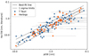 |
Fig. 1. Correlation between H equivalent widths from medium-resolution spectra and Gaia H pseudo-equivalent widths, for a sample of YSOs (T Tauri and Herbig stars). The black lines represent the best linear fit to the data and its uncertainties, log(−EWHα) = (1.13 ± 0.04)⋅log(−pEW)+(0.41 ± 0.02)±0.18. |
2.3. Derivation of the H-alpha line flux
To convert EWHα into a H line flux, it is necessary to know the continuum flux density at the H line (Fcont). For the YSOs with XP spectra available, Fcont can be obtained from the spectra using linefinder (Weiler et al. 2023). We combined the YSOs from the Sco-Cen star-forming region identified in Ratzenböck et al. (2023a) that have have pEW < − 0.5 nm with the T Tauri stars from Manara et al. (2023) and the Herbig stars from Fairlamb et al. (2015). We selected the sources with XP spectra, ran linefinder without truncation on their spectra and then selected the sources for which linefinder reports values with depthlf > 10−17 W/nm/m2 and widthlf < 25 nm. We selected these values to reduce the number of potentially misclassified H emitters (see Appendix B). The resulting sample contains 114 sources.
We then calculated Fcont = fluxlf − depthlf. We obtained uncertainty estimates for Fcont by setting the errors equal to the difference between the values of Fcont calculated using linefinder when truncating the coefficients which represent the spectra to a recommended value and when not truncating them. We also set the errors to a minimum of 10% as a conservative estimate. We then fit a relation between Fcont and the Gaia DR3 mean magnitude in the integrated RP band (RP), assuming an error of 5% for RP. We fit a relation of the form
 (3)
(3)
where a and b are the regression coefficients, and ϵ2 is used to account for the intrinsic random scatter. Using a Bayesian method to account for errors (Kelly 2007), we obtained the values of a and b, with errors, and of the error from the intrinsic scatter, σϵ2 (see Table 1). The plot of the correlation is shown in Appendix C. We used this relation to derive Fcont from Gaia RP for all sources in our original dataset with pEW < − 0.5 nm. Then, we derived the H line flux as FHα = EWHα ⋅ Fcont. The uncertainties on the fit parameters and RP and the intrinsic scatter were propagated consistently through bootstrapping. The median value as well as the 16th and 84th percentiles were calculated for both Fcont and FHα, and they are presented in Table 2.
Parameters derived in this work from Gaia XP spectra and pEW for H emitters within 500 pc (145 975 sources).
2.4. Accounting for interstellar extinction
In the approach presented in Sect. 2.3 for deriving the H line flux FHα, interstellar extinction is not taken into account. We repeated the derivation of FHα two more times. First, we accounted for extinction using the broadband extinction provided as part of Gaia DR3. The Gaia DR3 astrophysical_parameters table provides the broadband extinction in the Gaia passbands inferred by the General Stellar Parametrizer from Photometry Aeneas using BP/RP spectra, apparent G magnitude and parallax (Andrae et al. 2023, GSP-Phot extinction).
However, only 68% of the sample of 145 975 sources with pEW< − 0.5 nm has GSP-Phot extinctions. For this reason, we also estimated interstellar extinctions by taking the median value of the GSP-Phot extinctions of neighbouring stars (‘med-GSP-Phot extinction’). We did this for 99% of the sample, which have at least one other source within a 5 pc radius sphere (94% of them have five or more sources in this volume).
We calculated the extinction-corrected RP magnitude as RPcorrected = RP − ARP, where ARP is the extinction in the corresponding band. Upper and lower limits for RPcorrected were obtained by considering the uncertainty in ARP. This uncertainty is provided by Gaia DR3 in the case of GSP-Phot extinctions, and we took the mean of the 25th and 75th percentile errors as the uncertainty in med-GSP-Phot extinctions. We obtained the extinction-corrected continuum flux from the equation:
 (4)
(4)
We repeated the fit from Sect. 2.3 (Eq. (3)), using values of RPcorrected and Fcont,corrected, extinction-corrected with GSP-Phot and with med-GSP-Phot extinctions. The values of the parameters relating the continuum flux density at the H line with the RP magnitude under these extinction corrections are reported in Table 1, and the plot of the relation between the two quantities can be found in Appendix C. We then obtained new values of FHα for all sources with pEW < − 0.5, using the two extinction estimations, propagating errors through bootstrapping (Table 2).
2.5. Derivation of stellar parameters
We estimated stellar parameters for the sample of 145 975 stars within 500 pc and with pEW < −0.5 nm (stellar masses, effective temperature, stellar luminosities, stellar radii, and surface gravities). For this, we used the extinction estimations of the previous section. We corrected the Gaia GBP-GRP colours from extinction, and derived absolute MG magnitudes by using the geometric distances of Bailer-Jones et al. (2021). We then placed our sources in the dereddened colour-magnitude diagram (CMD), from where we derived stellar parameters using theoretical evolutionary tracks. We used the Baraffe et al. (2015) tracks which are optimised for pre-main sequence and main sequence low-mass stars (extending to 1.4 M⊙). Stellar parameters were derived assuming both GSP-Phot extinction and med-GSP-Phot extinction. We set the errors in the colour-magnitude diagram to be at minimum 0.1 mag in colour and in absolute magnitude. This decision is due to the fact that Gaia uncertainties are sometimes underestimated, producing unrealistically accurate positions in the CMD. Measured stellar parameters for both sets of extinction corrections are presented in Table 2. Sources outside of the Baraffe et al. (2015) tracks in the CMD have no stellar parameters associated. Therefore, stellar parameters calculated from GSP-Phot extinction are available for a total of 80 348 stars, and stellar parameters calculated from med-GSP-Phot extinction are available for a total of 140 083 stars.
2.6. Accretion luminosities and mass accretion rates
The H line luminosity can be obtained as LHα = 4πd2 ⋅ FHα, where d is the geometric distance from Bailer-Jones et al. (2021). The accretion luminosity can be derived as:
 (5)
(5)
where A and B are constants. We used A = 1.13 ± 0.05 and B = 1.74 ± 0.19, which are the values determined in Alcalá et al. (2017) for classical T Tauri stars. Using this equation and the results of Sects. 2.3 and 2.4, we derived accretion luminosities for all sources in our sample and for the three extinction regimes described in Sect. 2.4 (no extinction, GSP-Phot extinction, and med-GSP-Phot extinction).
Following the approach presented in Alcalá et al. (2017), we converted the accretion luminosities into mass accretion rates, Ṁacc, using the relation
 (6)
(6)
where R⋆ and M⋆ are the stellar radius and mass, respectively, and Rin is the inner-disc radius, which as in Alcalá et al. (2017) we assumed to be Rin = 5R⋆ for comparison with previous results. We calculated mass accretion rates for all sources with pEW < − 0.5 nm, correcting for extinction with both GSP-Phot extinction and med-GSP-Phot extinction. We note that Equations (5) and (6) assume magnetospheric accretion and that the H emission component is tracing the accretion flows (Hartmann et al. 2016).
All errors, including those of the distance, of constants A and B, of the stellar parameters, and of all initial quantities and fit parameters, as well as the intrinsic scatter in the relationships, discussed in the previous sections were propagated consistently to the final values of Lacc and Ṁacc through bootstrapping with 1000 steps. For each value we report the median and the 16th and 84th percentiles.
In summary, we produced a table of accretion luminosities and mass accretion rates for all 145 975 sources within 500 pc with pEW < − 0.5 nm, excluding the sources with linefinder-measured widthlf > 25 nm. An extract of the table is presented in Table 2, and the full table is available as online material.
2.7. Criteria for identifying YSOs
Various filters can be considered to refine Table 2 and select purer samples of YSO candidates. However, each filter introduces a noticeable selection bias towards a certain population of YSOs. Table 2 (Sects. 2.1–2.6 and Appendix B) is intended to be the most general compilation of YSO H emitter candidates within 500 pc that can be gathered from Gaia XP spectra. We added different ‘quality flags’ to Table 2 that users might want to apply, or not, depending on each individual science case (see e.g. Sects. 3.2 and 4). A graphic representation of the full decision tree used to build Table 2 and its different quality flags is presented in Fig. 2. We dedicate this section to explain these quality flags.
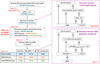 |
Fig. 2. Diagram illustrating the various selections applied to the original sample of all Gaia DR3 sources within 500 pc with measured pEW to obtain the final sample of YSO candidates (Table 2), and the different quality flags that can be applied to further refine the purity of the sample. The two boxes on the right show two of the steps in more detail. |
First, we used Gaia photometry to remove sources outside of the YSO locus in the colour-magnitude diagram (Fig. 3). The YSO locus we defined is reported in Appendix D. This removed 1494 sources from the sample that are incompatible with a YSO location in the CMD. Sources within the YSO-compatible region are flagged in Table 2 as ‘flag_CMD’. To compare with other YSO catalogues, ∼35 000 sources of the resulting sample with ‘flag_CMD’ are contained in the Marton et al. (2019) catalogue, and ∼25% of the Marton et al. (2023) sample of variable YSO candidates is contained in our sample with ‘flag_CMD’ (when limited to 500 pc and considering only sources with XP spectra). To further identify YSOs in the ‘flag_CMD’ sample, we propose three different selection criteria:
-
Filter by infrared (IR) excess signalling the presence of protoplanetary discs: We performed a 2 arcsecond cross-match of Gaia DR3 co-ordinates with AllWISE (Cutri et al. 2021), which contains both 2MASS and WISE photometries. We selected the sources that show an IR excess similar to the one produced by protoplanetary discs in known YSOs. In particular, we selected sources that have J − Ks > 0.60 mag and W1 − W2 > 0.25 mag (excluding upper limits), as is shown in Fig. 4. With this selection, we retained 95% of the YSOs from Manara et al. (2023). This IR cut produces an all-sky sample of 4208 sources (Fig. 6). We did not use W3 and W4 because their lower angular resolution often results in source blending in crowded regions, producing false positives. We note that applying this filter biases the selection towards sources with a significant amount of re-radiated emission from their protoplanetary discs, and against sources with discs which produce weak or no excess in the near IR (e.g. sources with large cavities). Indeed, we observe high accretion luminosities for sources in the IR excess regime selected by this filter (Fig. 4.), independently suggesting that the selection is biased towards more massive discs (Manara et al. 2016a). Sources that satisfy this filter have the ‘flag_IR’ quality flag in Table 2.
-
Filter by pEW < − 1 nm: In Sect. 2.1 (see also Appendix B) we find pEW < − 1 nm is the pEW threshold which achieves the best balance between number of sources and reliable YSO H emitters. We note that applying this filter biases the selection towards sources with stronger H emission. For this quality flag, we also introduced an additional criterion to account for the non-homogeneous distribution in the sky of public XP spectra due to the Gaia scanning law (Sect. 2.6). For the sources without XP spectra, we manually selected those that fall in the regions with poor Gaia coverage and only keep those that have log(Lacc,med-GSP-Phot extinction/L⊙) > − 3.5. This threshold is discussed in more detail in Appendix E. This filter produces an all-sky sample of 6170 sources (Fig. 6), and retains 69% of the YSOs from Manara et al. (2023). Sources that satisfy this filter have the ‘flag_pEW’ quality flag in Table 2.
-
Combining A and B: We applied both A and B criteria to produce a very pure sample of YSOs. By doing this, we obtained an all-sky sample of 1945 sources (Fig. 6), and we retained 60% of the YSOs from Manara et al. (2023). Sources that satisfy this filter have the ‘flag_combined’ quality flag in Table 2.
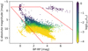 |
Fig. 3. Colour-magnitude diagram (CMD) of all H emitter candidates within 500 pc (Table 2). The 1494 sources outside of the red lines are flagged in Sect. 2.7 as being incompatible with a YSO location in the CMD. The equations to reproduce the lines are reported in Appendix D. The sources are colour-coded by accretion luminosity, using the accretion luminosity calculated using med-GSP-Phot extinction. Grey sources belong to the 1% of the sample which does not have med-GSP-Phot extinction. |
We note that, while the flag on IR excess (criterion A, Fig. 4) should be used when aiming for a low-contamination sample of sources with a significant amount of emission in the near IR, it does not imply that all sources where this flag is false do not have IR excess. Two main factors may cause sources with IR excess to have ‘flag_IR’ set to false. Firstly, the flag is false if the photometry in any one of J, Ks, W1 or W2 is an upper limit. Secondly, IR excess could begin at longer wavelengths. For example, if we consider the 6170 sources of sample B (sources with strong H signatures, ‘flag_pEW’), only 32% have ‘flag_IR’. However, for 13% of sample B the flag is false due to upper limits. Additionally, from the remaining 3435 sources we take the 278 that have non-upper limit W3 and W4 magnitudes, and search for excess at longer wavelengths. We find that 90% have W3 − W4 > 1 (and 81% have W3 − W4 > 2). These numbers indicate that there is a large fraction of YSOs where the IR excess only starts at longer wavelengths, but we do not apply a selection at longer wavelengths due the quality of W3 and W4 photometry.
An additional quality flag is available in Table 2, labelled as ‘flag_above_chromospheric_level’. This flag indicates whether accretion is observed above the level of chromospheric emission, using the results from Manara et al. (2017a). If accretion is below this level, the measured accretion luminosity and mass accretion rate could be spurious detections incorrectly derived from chromospheric emission. We derived this flag for the whole sample of sources with med-GSP-Phot stellar parameters (96% of the total sample of Table 2), and found that 55% of sources are below the chromospheric emission level. We then checked how many sources in each of samples A, B, and C are below this level (Fig. 5). For sample A, 8.44% of the sample is located below the locus of chromospheric emission lines, indicating some degree of contamination. For sample B, only 0.15% is located below the locus, and for sample C, no sources in the sample (save two) are below the locus. This is a strong indication that all sources in sample C are indeed true YSO accretors.
Fig. 6 shows the three resulting samples from filters A, B, and C plotted in galactic co-ordinates, and colour-coded by their accretion luminosity. In all three cases, the regions of stronger accretion correspond to known star-forming regions, but there is a population of low-accreting disperse YSOs. Zooming into star-forming regions and plotting them on the Planck 217 GHz map (Planck Collaboration III 2020) shows the spatial distribution of YSOs following the structure of dust (Fig. 8). While not shown here, a similar structure is observed when colour-coding by mass accretion rate. Fig. 7 shows a histogram of the distances of YSO candidates including the full table with ‘flag_CMD’ and samples A, B, and C. For A, B, and C the distribution shows two peaks, the first corresponding mostly to the Sco-Cen and Taurus regions, and the second to Orion. The table with ‘flag_CMD’ shows no sign of structure as a function of distance. This illustrates the importance of applying at least one of the quality cuts described in this section for retrieving pure YSO populations.
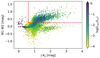 |
Fig. 4. Colour-colour plot using 2MASS and WISE magnitudes. The sources in the plot were pre-selected using the colour-magnitude diagram of Fig. 3, and by excluding upper limits. The region to the top right (J − Ks > 0.60 mag and W1 − W2 > 0.25 mag) is the region considered when applying selection criterion A (Sect. 2.7). The sources are colour-coded by accretion luminosity, using the accretion luminosity calculated using med-GSP-Phot extinction. Grey sources belong to the 1% of the sample which does not have med-GSP-Phot extinction. |
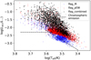 |
Fig. 5. Accretion luminosity divided by stellar luminosity as a function of effective temperature for the all-sky YSOs with accretion luminosity and effective temperature calculated from med-GSP-Phot extinction, from samples A (flag_IR, 4086 sources), B (flag_pEW, 5934 sources), and C (flag_combined, 1871 sources). All sources from sample C are, by definition, also included in sample A and B. Dashed lines trace the locus of chromospheric emission lines when they are erroneously converted into accretion luminosities, as derived in Manara et al. (2017a). 8.44% of sample A and 0.15% of sample B are below the chromospheric emission lines. |
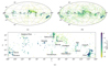 |
Fig. 6. Fig. (a): Sky plot in galactic co-ordinates of YSO H emitters selected using criterion A (filtering by IR excess, Sect. 2.7). Fig. (b): Sky plot in galactic co-ordinates of YSO H emitters selected using criterion B (filtering by pEW). Fig. (c): Sky plot in galactic co-ordinates of YSO H emitters selected using criterion C, which is the intersection of sources in A and B. In Fig. (c), the plot is zoomed in around the Galactic plane. The star-forming regions are labelled following Avedisova (2002). The sources are colour-coded by their accretion luminosity calculated using med-GSP-Phot extinction (Sect. 2.4). The few sources without med-GSP-Phot extinction are shown in grey. |
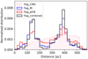 |
Fig. 7. Histogram of distances of YSO H emitter candidates including the full table with ‘flag_CMD’ and samples A, B, and C (these being refined subsets of YSO candidates, Sect. 2.7). We use the geometric distances of Bailer-Jones et al. (2021). |
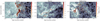 |
Fig. 8. Detail of some star-forming regions from Fig. 6 bottom panel (sample C), plotted over the Planck map at 217 GHz (Planck Collaboration III 2020). YSOs with higher accretion luminosities can be appreciated concentrated in the more clustered areas, following the structure of the regions. |
2.8. Comparison with literature values of accretion luminosity and mass accretion rate
We compared the accretion luminosities and mass accretion rates derived in Sect. 2.6 with the accretion properties of the sample of known classical T Tauri stars from Manara et al. (2023, and references therein). We have 341 YSOs in common, and the sample contains objects from various regions within 300 pc, including Lupus, Taurus, Ophiuchus, Chamaeleon I, Chamaeleon II, Corona Australis, and Upper Scorpius. The stellar and accretion parameters provided by Manara et al. (2023) were mainly obtained from surveys carried out with the VLT/X-Shooter instrument (R ∼ 10 000). Fig. 9 shows the comparison of our accretion luminosities and mass accretion rates with these literature values from higher-resolution spectroscopy, for the different extinction corrections considered in this work (Sect. 2.4).
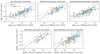 |
Fig. 9. Comparison of the accretion luminosities and mass accretion rates of this work with the values reported in Manara et al. (2023) from higher-resolution spectroscopy. The dashed black lines are the 1:1 lines, and the dashed grey lines show ±1 dex. Top panels: Three plots showing accretion luminosities calculated without accounting for extinction (left), using Gaia GSP-Phot extinction (central), and using med-GSP-Phot extinction (right). Bottom panels: Two plots showing mass accretion rates calculated using Gaia GSP-Phot extinction (left), and using med-GSP-Phot extinction (right). |
Fig. 9 shows that the accretion luminosities and mass accretion rates estimated from the Gaia XP spectra are accurate to within an order of magnitude, when extinction is taken into account. A better match is found for the GSP-Phot extinction correction than for the med-GSP-Phot extinction correction. This is expected, as circumstellar extinction is an important component of the extinction in YSOs and med-GSP-Phot, by definition, only traces interstellar extinction (and hence systematically supposes a lower limit to the real extinction, Sect. 2.4). Because of this, med-GSP-Phot based accretion luminosities and mass accretion rates tend to underestimate the values obtained from higher-resolution spectroscopy. We note, however, that med-GSP-Phot extinctions are available for 99% of the original sample of H emitters within 500 pc, as opposed to the 68% in the case of GSP-Phot extinctions (Sect. 2.4). This is why med-GSP-Phot based accretion luminosities were used in Figs. 3, 4, 5, 6, and 8. pEW < − 1.0 nm sources are indicated in Fig. 9 to illustrate the behaviour of the accretion parameters derived from XP spectra when using criterion B for selecting a purer sample of YSO H emitters (Sect. 2.7).
The lower limit to the mass accretion rate that we are sensitive too is Ṁacc ∼ 10−12 M⊙/yr, or log(Lacc/L⊙)∼ − 5.0 in the case of accretion luminosity. These lower detection limits are inferred because in the comparison with literature values the latter are all above these limits (Fig. 9), and the distribution of accretion properties for the whole set of H emitters drops abruptly at these limits (see Sect. 3.2).
3. All-sky view of YSO accretion
In this section, we present an all-sky homogeneous view of YSO accretion within 500 pc, using the accretion properties we obtained from Gaia XP spectra (Table 2). We analyse the sky distribution of YSO accretion and correlate accretion properties to stellar parameters.
3.1. Distribution of accretion luminosities and mass accretion rates
In Fig. 10 we show the distribution of accretion luminosities and mass accretion rates derived in Sect. 2.6 for YSO H emitters within 500 pc with the quality filters of Sect. 2.7 (see Fig. 2). For comparison purposes we have added to this plot the accretion luminosities and mass accretion rates presented in Manara et al. (2023) for well-characterised T Tauri stars from higher-resolution spectroscopy.
Fig. 10 shows that the literature sample of T Tauri stars with well-described accretion properties (i.e. Manara et al. 2023 sample) consists of stronger accretors than our YSO samples. While it is likely that the ‘flag_CMD’ peak at log(Lacc/L⊙)∼ − 4 in Fig. 10 is affected by the presence of non-YSO contaminants (Sect. 2.7), the ‘flag_IR’ and ‘flag_pEW’ selections also peak at this low-accretion regime, suggesting a population of YSO low accretors largely untraced by previous spectroscopic surveys. Moreover, previous spectroscopic surveys are well contained by our IR excess selection (‘flag_IR’), indicating a bias of previous studies towards YSO accretors with IR-bright protoplanetary discs.
We note that the YSO populations of H emitters identified in this work also have different distributions depending on the filtering criteria we apply. The cumulative distributions of Fig. 10 indicate that demanding a certain level of IR excess tends to favour stronger accretors more efficiently than demanding a certain level of pEW. This is particularly evident for the strongest accretors with log(Lacc/L⊙) > − 2. We believe this to be a consequence of two effects: more massive discs are correlated with stronger accretion (Manara et al. 2016a), and discs disperse with time while accretion also diminishes with time (Fedele et al. 2010; Ribas et al. 2015, see also Sect. 4). The previously described effects are even more notorious when considering the mass accretions rates (albeit these are more uncertain in this work, as they have a higher dependence on extinction and stellar parameters).
As is described in Sect. 2.8, the med-GSP-Phot based accretion properties are systematically underestimated. This can also be appreciated in Fig. 10. Nevertheless, similar trends as observed for GSP-Phot based accretion properties can be observed for the larger sample of objects with accretion properties derived using med-GSP-Phot. The two peaked profile distribution of GSP-Phot based accretion luminosities is a direct consequence of the two peak extinction profile reported by Gaia GSP-Phot (Andrae et al. 2023) for the same sample of sources. This is an artifact of the GSP module, which tends to overestimate extinctions for sources with notable extinction3. The two-peak distributions indeed transform into smooth distributions when averaging the extinction of several sources (using med-GSP-Phot). Because of this we did not derive stellar parameters (and hence mass accretion rates) for sources that fall outside of the Baraffe et al. (2015) tracks in the dereddened CMD (Sect. 2.5). This explains the absence of a double-peaked distribution in the mass accretion rates calculated with GSP-Phot, as sources with slightly overestimated extinctions fall outside of the Baraffe et al. (2015) tracks.
Fraction of accreting stars, median accretion luminosity, and median mass accretion rate for 34 Sco-Cen clusters.
The sky distribution of the YSO low accretors can be observed in Fig. 6, where it is noticeable that the population of low accretors is mostly dispersed, away from star-forming regions or clustered environments of star formation. Even within star-forming regions, the YSO low accretors appear disperse and separated from the more clustered areas, where the accretion luminosities are higher (Fig. 8). This spatial correlation of accretion, with higher accretors appearing more clustered and structured, can be related to ongoing infall from the interstellar medium onto the protoplanetary discs (Kuffmeier et al. 2023; Gupta et al. 2024; Winter et al. 2024a), star-disc encounters in denser areas (Winter et al. 2024b), evolution of YSOs with time towards isolation (Vioque et al. 2023), or ejected YSOs because of multiple system disruptions (Cournoyer-Cloutier et al. 2024). It is also worth noting that there is a small known population of very old (> 20 Myr) still accreting M-type YSOs (know as ‘Peter Pan’ discs, Silverberg et al. 2020) whose protoplanetary discs are likely primordial (Long et al. 2025). Coleman & Haworth (2020) predicted these sources should form in the periphery of low-mass star-forming regions or in more isolated locations. It could then be that a fraction of the population of field YSO low accretors we detect are old YSOs with surviving primordial discs that move from their little-crowded forming places.
3.2. All-sky view of accretion properties versus stellar parameters
Several relations have been found between the accretion properties of YSOs, their stellar parameters, and the properties of their protoplanetary discs, which have been used to describe the evolution of YSOs, their accretion mechanisms, and the transport of angular momentum in protoplanetary discs (see Manara et al. 2023 and references therein). In particular, stellar luminosities are known to positively correlate with accretion luminosities, and stellar masses to positively correlate with mass accretion rates. In this section we revisit these correlations with the largest sample ever considered of YSOs, homogeneously obtained for the whole sky.
In order to minimise the number of contaminants, we took sample C (‘flag_combined’, Sect. 2.7), which consists of 1945 sources. From these, we considered the 656 sources for which we have derived stellar parameters, accretion luminosities, and mass accretion rates from GSP-Phot extinction. We then looked at the correlation of accretion luminosity with stellar luminosity and mass accretion rate with stellar mass, shown in Fig. 11. Fitting the logarithmic relation between accretion luminosity and stellar luminosity (using the Bayesian method from Kelly (2007) to account for uncertainties in both quantities), we obtained Lacc ∝ L⋆1.41 ± 0.02. We then looked for a correlation between mass accretion rate and stellar mass, shown in Fig. 11. As we have no empirical calibration for sources with Ṁacc < 10−12 M⊙/yr, we exclude the sources in this limit. We set a conservative upper limit of 1.0 M⊙ for the fit to avoid entering the massive end regime of the Baraffe et al. (2015) tracks (Sect. 2.5). We fit a logarithmic relation, again accounting for uncertainties, and obtained that  . We repeated the procedure for the samples A and B of YSOs (respectively, ‘flag_IR’ and ‘flag_pEW’), and again repeated it using the values calculated using med-GSP-Phot extinction (we note that for med-GSP-Phot extinction we did not impose any constraints on the stellar mass). Fig. 11 shows med-GSP-Phot values in blue for the sources of sample C that do not have GSP-Phot extinction. The results of the fit for the different samples and extinction regimes are tabulated in Table 3. Comparing the values of the slopes in the logarithmic plane calculated with the different methods, we find a standard deviation of 0.05 for the Lacc − L⋆ relation and of 0.13 for the Ṁacc – M⋆ relation. The different methods therefore give consistent results, especially for the Lacc − L⋆ relation.
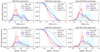 |
Fig. 10. Distribution of accretion luminosities and mass accretion rates derived for YSO H emitters within 500 pc. Different lines trace the quality filters described in Sect. 2.7 (see Fig. 2). The left panels present accretion properties obtained using the GSP-Phot extinction correction and the right panels the ones obtained using the med-GSP-Phot extinction correction (Sect. 2.4). We have added to this plot the accretion luminosities and mass accretion rates presented in Manara et al. (2023) for well-characterised T Tauri stars from higher-resolution spectroscopy. The central panels are cumulative distributions of the accretion properties shown on left panels, using GSP-Phot extinction. |
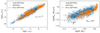 |
Fig. 11. Left: Accretion luminosity vs. stellar luminosity for 1871 YSOs all-sky within 500 pc (sample C, Sect. 2.7). The 655 sources of the sample that have GSP-Phot extinction are plotted according to their values of accretion luminosity and stellar luminosity derived using this extinction. The black line is the fit for the GSP-Phot values of these 656 sources. The value of the slope in the log-log plane is 1.41 ± 0.02. The remaining sources of sample C that do not have GSP-Phot extinction are plotted using the values calculated using med-GSP-Phot. The results of fitting to values calculated with med-GSP-Phot are reported in Table 3. Right: Mass accretion rate vs. stellar mass for the same sample of 1871 YSOs. The 656 sources of the sample that have GSP-Phot extinction are plotted according to their values derived using this extinction. The black line is the fit to the GSP-Phot values, for sources with stellar mass M⋆ < 1.0 M⊙, and with Ṁacc > 10−12 M⊙/yr. The value of the slope in the log-log plane is 2.4 ± 0.1. Again, the sources of sample C that do not have GSP-Phot extinction are plotted using the values calculated using med-GSP-Phot. |
We now compare the parameters of Table 3 with those found in previous studies. In this comparison, we note that we are tracing a different population of YSOs (Fig. 10), and that different stellar evolutionary models might have been used to obtain stellar parameters (this does not affect Lacc). For the Lacc – L⋆ correlation in the logarithmic plane, our values are in the range 1.41–1.57 for the slope and between −1.42 and −1.16 for the intercept, with best values (those of sample C with GSP-Phot extinction) of 1.41 ± 0.02 and −1.19 ± 0.02, respectively. Almendros-Abad et al. (2024) fit the power law correlation for sources in four different star-forming regions. For the Lacc – L⋆ relationship, they find values of the slope in the logarithmic plane in the range 1.19 to 1.76, and intercept in the range −1.65 to −1.1. Our values all fall within this range. Manara et al. (2017b) find a slope of 1.9 ± 0.1, and Tilling et al. (2008) present a theoretical study which uses simplified stellar evolution calculations for stars subject to a time-dependent accretion history, obtaining a slope of 1.7. Compared to the latter two studies, we find a flatter power law. For the Ṁacc – M⋆ correlation, we obtain values of the slope in the range 2.19 to 2.5, and of the intercept in the range −9.72 to −8.66, with best (sample C) values of 2.4 ± 0.1 and −8.93 ± 0.05. Our power law is within error of the one found in Manara et al. (2017b), which has a slope of 2.3 ± 0.3, but slightly steeper than that of Almendros-Abad et al. (2024), where they find slopes in the range 1.33 to 2.08 (and intercept in the range −9.17 to −7.76). In conclusion, our Lacc – L⋆ correlation is consistent with the results of Almendros-Abad et al. (2024), while the Ṁacc – M⋆ power law is broadly consistent with Manara et al. (2017b) but steeper than the one found in Almendros-Abad et al. (2024).
4. Evolution of YSO accretion with age
4.1. Evolution of accretion with age in Sco-Cen
In this section, we analyse how the accretion of material in YSOs, from the protoplanetary discs onto the forming stars, evolves with age. However, YSO ages are notoriously hard to characterise, often being highly model dependent and uncertain (e.g. Soderblom 2010; Miret-Roig et al. 2024; Rottensteiner & Meingast 2024). To circumvent this limitation, we considered the work of Ratzenböck et al. (2023b), who have derived ages homogeneously for 37 clusters in the Sco-Cen star formation complex (identified in Ratzenböck et al. 2023a). Therefore, the ages presented in this section might suffer from uncertainty and model systematics in absolute terms, but relative ages are more precise and they allow us to compare the accretion properties of clusters through YSO evolution. We discarded the clusters ‘Norma-North’, ‘Oph-Southeast’, and ‘Oph-NorthFar’ as these are found in Ratzenböck et al. (2023b) to be unrelated to Sco-Cen. We note that the classical old regions of Upper-Centaurus-Lupus (UCL), and Lower-Centaurus-Crux (LCC) appear here subdivided into smaller groups (Ratzenböck et al. 2023a).
The 34 Sco-Cen stellar clusters identified in Ratzenböck et al. (2023a) contain a total of 12 972 stars. Ratzenböck et al. (2023b) provide four age estimates for each cluster, determined with two different evolutionary models, PARSEC v1.2S (Bressan et al. 2012) and that presented in Baraffe et al. (2015), and using two different colour-magnitude diagrams, (MG vs. GBP − GRP) and (MG vs. G − GRP). In this work we used the ages from Baraffe et al. (2015) models and MG versus GBP − GRP, but for consistency we examined that similar results are obtained using the other three age estimates. We cross-matched the members of the 34 clusters with our table of accretion properties and stellar parameters (Table 2). Fig. 12 shows the three-dimensional spatial distribution of the 1954 members of Sco-Cen for which we have calculated an accretion luminosity using med-GSP-Phot extinction, colour-coded by accretion luminosity. As in Sect. 3.1, in Sco-Cen a clear spatial differentiation in accretion strength can be appreciated, with some small regions concentrating the higher accretors, and with the more dispersed YSOs being mostly low accretors.
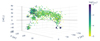 |
Fig. 12. Three-dimensional spatial distribution of 1954 members of the 34 Sco-Cen clusters identified by Ratzenböck et al. (2023a), colour-coded by accretion luminosity. The co-ordinates are provided in Ratzenböck et al. (2023a) and are such that the Sun is at (0,0,0) and the Z = 0 plane is parallel to the Galactic plane. For better visualisation, see the interactive 3D version online. |
For each cluster, we measured the number (Nacc) of sources that have pEW < − 1.0 nm in Table 2. Similarly to what we did to obtain sample B (Sect. 2.7), pEW < − 1.0 nm allows us to obtain a sample of accreting YSOs that includes fewer contaminants, providing the best compromise between accuracy and completeness (Appendix B). We then determined the total number (N) of sources in each cluster that have pEW values, and from this we calculated the fraction of sources per cluster with pEW < − 1.0 nm. We refer to this fraction as the fraction of accretors per cluster, facc. We estimated the uncertainty in facc as  , following Fedele et al. (2010). The values of facc of each cluster are presented in Table 4.
The top panel in Fig. 13 shows the fraction of accretors per cluster as a function of cluster age. We fit the observed decay in facc with age with two different functions: an exponential decay of the form
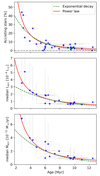 |
Fig. 13. Evolution of accretion in Sco-Cen clusters with age. Each point represents one of the 34 Sco-Cen clusters whose ages were calculated in Ratzenböck et al. (2023b). The ages shown here are the Baraffe et al. (2015) Bp-Rp ages of that work. In each panel, we show two fits: an exponential decay (Eq. (7)) and a power law (Eq. (8)). Top panel: we show the percentage of YSO accretors per cluster facc. The accretion timescale obtained from fitting the exponential is τacc = 2.7 ± 0.4 Myr. Bottom two panels: median accretion luminosity and the median mass accretion rate of the accretors (sources with pEW < − 1.0 nm) in each cluster. Only the cluster members with stellar mass in the range 0.08 < M⋆ < 0.25 M⊙ were considered for the medians, to remove dependencies with stellar mass. Only clusters with four or more accretors in this mass range were considered. All fit parameters are reported in Table 5. |
 (7)
(7)
and a power law of the form
 (8)
(8)
where t is the age in millions of years. Both fits were performed using the method from Kelly (2007), accounting for uncertainties in facc and for a conservative 20% error in the ages. Values of the parameters of the fits and of the reduced χ2 squared values are reported in Table 5. Based on the χred2 values as well as visual inspection of the fits, it appears that a power law is a better fit for the evolution of the fraction of accretors, although the value of the parameter k means that the fit might not be valid at ages lower than the range we consider. For comparison with literature, we report the value of the accretion timescale obtained from the exponential decay, which is τacc = (2.7 ± 0.4) Myr. This result is within error of the mass accretion timescale of 2.3 Myr calculated in Fedele et al. (2010) using a similar approach on a smaller dataset. From the results of our power law fit, we calculate that the percentage of accretors is 70% at 2 Myr and 2.8% at 10 Myr. This is similar to Fedele et al. (2010) which reports 60% and 2%, respectively. We detect 22 very old accretors (in regions with age > 10 Myr), which is 3.7% of the total number of accretors in Sco-Cen.
Fit parameters for the evolution of fraction of accretors (facc), median Lacc of the accretors and median Ṁacc of the accretors in Sco-Cen clusters with age, where by accretors we mean sources with pEW < − 1.0 nm.
In addition to the fraction of accretors at different ages, we analysed the evolution of the median accretion luminosity and mass accretion rate of the accretors in each cluster as a function of cluster age. To ensure that we were tracing real accretion, we again only considered the sample of sources that have pEW < − 1.0 nm. For this analysis, we used the values calculated with med-GSP-Phot extinction, because while values calculated with GSP-Phot extinction better correlate with literature values (Sect. 2.8) they are only available for 28% of the Sco-Cen sample. Therefore, to consider a large enough number of sources per cluster for running a statistical analysis, we chose to use med-GSP-Phot extinction corrected values (available for 98% of the sample), keeping in mind that they represent a consistent lower limit to the literature values.
Before proceeding with the analysis, we first had to evaluate any dependence with stellar mass, as it strongly correlates with accretion (Fig. 11). Using the stellar parameters derived in Sect. 2.5 (Table 2 from med-GSP-Phot extinctions, we observe differences between the median stellar mass of each of the Sco-Cen clusters (Fig. 14). In particular, we observe significant higher median stellar masses in Chameleon I and II. This difference is also present if the stellar masses derived from spectroscopy from Manara et al. (2023) are considered. We believe this is due to the fact that Chameleon I and II are some of the most Southern regions, making the populations harder to observe for most observatories. This is particularly relevant for faint sources, causing their observed populations to have higher median mass values than other regions. To avoid tracing the effect of stellar mass on accretion, we only considered the sources with stellar mass between 0.08 M⊙ and 0.25 M⊙ in every cluster. This forces the median stellar mass of all clusters to be similar. Then, for each cluster where there are at least four accretors in the chosen mass range, we calculated the median accretion luminosity and mass accretion rate. Uncertainties are given by the 16th and 8484 percentiles. Values of the medians, both corrected and uncorrected for stellar mass, can be found in Table 4. The evolution of the median accretion luminosity and mass accretion rate with age are shown in the bottom two panels of Fig. 13. We again fit an exponential decay function and a power law function, of the same form as the ones shown, respectively, in Eqs. (7) and (8). The results of these fits, performed with the approach from Kelly (2007) to account for errors, are reported in Table 5. As for the case of facc, the power law appears to better fit the data. The timescales, derived from the exponential fit, are larger than the one found for facc, but they also have large uncertainties. Comparing the values of α, the exponent of the power law, also shows that the evolution of median Lacc and median Ṁacc with time is slower than that of facc.
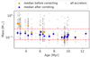 |
Fig. 14. Stellar mass distribution of accretors in the Sco-Cen clusters vs. cluster age (Baraffe et al. 2015-BpRp). The plot shows the stellar masses of all cluster members with pEW < − 1.0 nm as derived in Sect. 2.5 (Table 2), and the cluster median both before (orange) and after (blue) applying the 0.06 < M⋆ < 0.22 M⊙ cut (red lines). The median mass is only shown if there are at least four cluster members in the chosen mass range. We note this filtering by stellar mass results in similar median stellar masses for all clusters. |
Carpenter et al. (2025) compared millimetre-wavelength observations with the Ratzenböck et al. (2023a,b) cluster membership in Upper Scorpius, and found no significant evolution of mm-fluxes with age. Indeed, Polnitzky et al. (2025) finds a significantly larger than 2.7 Myr disc dissipation timescale for the same Sco-Cen clusters considered in this work. This could suggest the presence of planet-forming discs containing dust-traps (e.g. Testi et al. 2022), for which significant primordial or second-generation dust-disc material could be still detected while accretion is below detection thresholds. Indeed, a larger fraction of discs with inner dust cavities has been tentatively reported at the later Upper Scorpius ages (Vioque et al. 2025).
A tentative steepening with time of the Mdisc-M⋆ relation has been proposed (e.g. Pascucci et al. 2016; Ansdell et al. 2017), although this steepening is contested due to the scatter in the data and the associated uncertainties (Testi et al. 2022; Manara et al. 2023). If this steepening is true, population synthesis models have predicted that for viscously evolving discs the Ṁacc-M⋆ correlation (Fig. 11) should also steepen with time (Somigliana et al. 2022). This would imply that the accretion timescale for low mass YSOs is shorter (i.e. they evolve faster) than for more massive YSOs. By taking the Sco-Cen clusters of Ratzenböck et al. (2023a,b) we can evaluate this change in steepness in the Ṁacc-M⋆ and Lacc-L⋆ power law relationships homogeneously for the whole Sco-Cen region (spanning ∼10 Myr). The results of fitting the two relations for the ten clusters of Sco-Cen with at least 20 sources for which we traced accretion (considering only the sources with pEW < − 1.0 nm to exclude contaminants, as in criterion B of Sect. 2.7) are presented in Fig. 15. The plots of the fits for each region, and the values of the slopes, can be found in Appendix F. For most clusters, the slopes we find are in the same range as those calculated in Almendros-Abad et al. (2024), which are discussed in Sect. 3.2. The correlations we find are not indicating any clear evolution with time of either the Ṁacc-M⋆ or the Lacc-L⋆ relations. We do not find significant gradient differences for clusters of very different ages. We note that in this analysis we do not apply any filtering on the mass range of cluster members. More accurate determinations of accretion rates for complete populations are needed to further explore these relations.
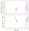 |
Fig. 15. Slope of the correlations of accretion luminosity vs. stellar luminosity (top panel), and mass accretion rate vs. stellar mass (bottom panel) for ten clusters of Sco-Cen, plotted against cluster age (Baraffe et al. 2015 Bp-Rp ages). For each cluster, we measured the slope of the correlations in the logarithmic plane, using values calculated with med-GSP-Phot, and only considering sources with pEW < − 1.0 nm. Only clusters where at least 20 sources could be used in the fit were considered. Each point is colour-coded to match the corresponding fit in Appendix F. |
4.2. Other star-forming regions
An implicit assumption of Sect. 4.1 is that all clusters within Sco-Cen can be considered as snapshots of the same star formation process, disregarding the impact of the environment or cluster-to-cluster intrinsic differences. While this assumption might be appropriate for the general derivations of Sect. 4.1 for the Sco-Cen complex, it can help explain some of the observed scatter. For example, external photoevaporation from massive stars has been proven to have a significant impact in Upper Scorpius gas-disc radii (Anania et al. 2025).
For legacy value, in this section we derive the fraction of accretors (facc), median accretion luminosity and median mass accretion rate for other known star-forming regions and groups (following the prescriptions of Sect. 4.1 and using Table 2). We report the derived values in Table 6, together with literature estimates of ages and the references for group membership.
Table 6 shows that older regions tend to have lower values of median accretion luminosity and mass accretion rate. The fraction of accretors (facc) per cluster also decreases with time, as illustrated in Fig. 16, where the regions of Table 6 are over-plotted on the top panel of Fig. 13. We note that the regions of Table 6 span very different environments and their ages come from different sources. In addition, they vary in distance and extinction and hence Gaia traces different YSO populations in them. Thus, Fig. 16 is only illustrative.
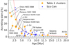 |
Fig. 16. Fraction of accretors against age for each region of Table 6, over-plotted on the top panel of Fig. 13. The Table 6 regions (orange stars in the plot) are labelled. The blue dots are the Sco-Cen clusters of Fig. 13 and the red and green line are, respectively, the power law and exponential fit to the Sco-Cen clusters, obtained in Sect. 4.1. |
Fraction of accreting stars, median accretion luminosity, and median mass accretion rate for various star-forming regions and groups within 500 pc.
5. Conclusions
We have presented an all-sky homogeneous analysis of the H emitting YSO candidates within 500 pc down to G magnitude 17.65 mag. By using the Gaia XP spectra, we have characterised the H line and derived accretion luminosities and mass accretion rates for a sample of 145 975 potential YSOs, which we present in Table 2, together with an estimation of the stellar parameters. We evidence the accuracy of our accretion determinations by comparing to accretion measurements derived from higher-resolution spectra. In Sect. 2.7 we describe filtering strategies to select specific sub-samples of YSOs from Table 2 that could be adopted for specific science cases.
We present some applications of this YSO catalogue for studying star formation in the solar neighbourhood. The main results we obtain after analysing this new sample of YSOs are:
-
While we recover well the known population of YSOs with measured accretion rates, we identify a large population of low-accreting YSO candidates previously untraced by YSO accretion rate surveys. Even when applying strict sample-purity constraints, we recover a significant population of accreting YSOs at Ṁacc = 10−11 to 10−12 M⊙/yr. We find previous accretion rate studies have mostly focused on the YSO population with significant infrared excesses from disc emission.
-
The population of low-accreting potential YSOs is mostly dispersed, away from star-forming regions or clustered environments of star formation. Even within star-forming regions, the YSO low accretors appear disperse and separated from the more clustered areas, where the accretion luminosities and mass accretion rates are higher. This could be due to the influence of the environment on star formation or YSO dispersion with age. Many low accretors appear entirely disconnected from young regions. This disperse population is likely to contain new ‘Peter Pan’ YSOs.
-
We evaluated the Ṁacc-M⋆ and Lacc-L⋆ relations for our sample of all-sky YSOs, finding values of Lacc ∝ L⋆1.41 ± 0.02 and
 . Both correlations are broadly consistent with literature values. In addition, we report the values of this relation for regions of different ages across the Sco-Cen complex, finding that the Ṁacc-M⋆ and Lacc-L⋆ correlations remain roughly constant in time.
 -
We analysed the decay of accretion rate with time by using the Sco-Cen complex cluster members and ages of Ratzenböck et al. (2023a,b, Table 4). By fitting an exponential function to the fraction of accreting stars in clusters of different ages, we obtain an accretion timescale of τacc = 2.7 ± 0.4 Myr. We find that a power law fits the evolution with age better than an exponential function and, using a power law fit, we find that the percentage of accretors is 70% at 2 Myr and 2.8% at 10 Myr. Moreover, we fit the exponential decay timescales of Lacc (τacc = 4.9 ± 3.0 Myr) and Ṁacc (τacc = 4.5 ± 2.4 Myr) of accreting sources. For all three cases, we report the results of fitting both the exponential function and the power law.
-
We report the fraction of accreting stars, median accretion luminosity and median mass accretion rate, for a collection of star-forming regions and groups within 500 pc (Table 6). We confirm the decay of accretion with age in theseregions.
This work constitutes the first effort to derive accretion rates for YSOs using the Gaia XP spectra. We have produced a sample of 145 975 nearby accreting YSO candidates, with 4 208 being more robust based on their IR excess, 6170 being more robust based on their H emission strength, and 1945 sources being the most robust, based on both factors. This work lays the foundations for improved analyses to be done with Gaia data release 4, and the publication of all the individual epochs of XP spectra. Other ongoing and future efforts to characterise in greater detail the extinction towards the different star-forming regions will also benefit the accuracy of future derivations.
Data availability
Full Tables 2, 4 and 6 are only available at the CDS via anonymous ftp to cdsarc.cds.unistra.fr (130.79.128.5) or via https://cdsarc.cds.unistra.fr/viz-bin/cat/J/A+A/699/A145
3D interactive figure associated to Fig. 12 is available at https://www.aanda.org
Acknowledgments
We thank the anonymous referee for their valuable comments and suggestions which improved the quality of the paper. We thank Giacomo Beccari, Carlo F. Manara, and Alice Somigliana for insightful discussions which improved this work. This job has made use of the Python package GaiaXPy, developed and maintained by members of the Gaia Data Processing and Analysis Consortium (DPAC), and in particular, Coordination Unit 5 (CU5), and the Data Processing Centre located at the Institute of Astronomy, Cambridge, UK (DPCI). This work has made use of data from the European Space Agency (ESA) mission Gaia (https://www.cosmos.esa.int/gaia), processed by the Gaia Data Processing and Analysis Consortium (DPAC, https://www.cosmos.esa.int/web/gaia/dpac/consortium). Funding for the DPAC has been provided by national institutions, in particular the institutions participating in the Gaia Multilateral Agreement. This research has made use of the TOPCAT interactive graphical tool (Taylor 2005). Additionally, this research has made use of the VizieR catalogue access tool, CDS, Strasbourg, France.
References
- Alcalá, J. M., Natta, A., Manara, C. F., et al. 2014, A&A, 561, A2 [NASA ADS] [CrossRef] [EDP Sciences] [Google Scholar]
- Alcalá, J. M., Manara, C. F., Natta, A., et al. 2017, A&A, 600, A20 [NASA ADS] [CrossRef] [EDP Sciences] [Google Scholar]
- Almendros-Abad, V., Manara, C. F., Testi, L., et al. 2024, A&A, 685, A118 [NASA ADS] [CrossRef] [EDP Sciences] [Google Scholar]
- Anania, R., Rosotti, G. P., Gárate, M., et al. 2025, AJ, accepted [arXiv:2506.10743] [Google Scholar]
- Andrae, R., Fouesneau, M., Sordo, R., et al. 2023, A&A, 674, A27 [CrossRef] [EDP Sciences] [Google Scholar]
- Ansdell, M., Williams, J. P., Manara, C. F., et al. 2017, AJ, 153, 240 [Google Scholar]
- Avedisova, V. S. 2002, Astron. Rep., 46, 193 [NASA ADS] [CrossRef] [Google Scholar]
- Bailer-Jones, C. A. L., Rybizki, J., Fouesneau, M., Demleitner, M., & Andrae, R. 2021, AJ, 161, 147 [Google Scholar]
- Baraffe, I., Homeier, D., Allard, F., & Chabrier, G. 2015, A&A, 577, A42 [NASA ADS] [CrossRef] [EDP Sciences] [Google Scholar]
- Bressan, A., Marigo, P., Girardi, L., et al. 2012, MNRAS, 427, 127 [NASA ADS] [CrossRef] [Google Scholar]
- Cantat-Gaudin, T., Fouesneau, M., Rix, H.-W., et al. 2023, A&A, 669, A55 [NASA ADS] [CrossRef] [EDP Sciences] [Google Scholar]
- Cao, L., Pinsonneault, M., Hillenbrand, L., & Kuhn, M. 2021, https://doi.org/10.5281/zenodo.4567677 [Google Scholar]
- Carpenter, J. M., Esplin, T. L., Luhman, K. L., Mamajek, E. E., & Andrews, S. M. 2025, ApJ, 978, 117 [Google Scholar]
- Carrasco, J. M., Weiler, M., Jordi, C., et al. 2021, A&A, 652, A86 [NASA ADS] [CrossRef] [EDP Sciences] [Google Scholar]
- Castro-Ginard, A., Brown, A. G. A., Kostrzewa-Rutkowska, Z., et al. 2023, A&A, 677, A37 [NASA ADS] [CrossRef] [EDP Sciences] [Google Scholar]
- Claes, R. A. B., Manara, C. F., Garcia-Lopez, R., et al. 2022, A&A, 664, L7 [NASA ADS] [CrossRef] [EDP Sciences] [Google Scholar]
- Cody, A. M., & Hillenbrand, L. A. 2018, AJ, 156, 71 [Google Scholar]
- Coleman, G. A. L., & Haworth, T. J. 2020, MNRAS, 496, L111 [NASA ADS] [CrossRef] [Google Scholar]
- Cournoyer-Cloutier, C., Karam, J., Sills, A., Zwart, S. P., & Wilhelm, M. J. C. 2024, ApJ, 975, 207 [Google Scholar]
- Creevey, O. L., Sordo, R., Pailler, F., et al. 2023, A&A, 674, A26 [NASA ADS] [CrossRef] [EDP Sciences] [Google Scholar]
- Cutri, R. M., Wright, E. L., Conrow, T., et al. 2021, VizieR Online Data Catalog: AllWISE Data Release (Cutri+ 2013), VizieR On-line Data Catalog: II/328. Originally published in: IPAC/Caltech (2013) [Google Scholar]
- De Angeli, F., Weiler, M., Montegriffo, P., et al. 2023, A&A, 674, A2 [NASA ADS] [CrossRef] [EDP Sciences] [Google Scholar]
- De Marchi, G., Panagia, N., & Romaniello, M. 2010, ApJ, 715, 1 [NASA ADS] [CrossRef] [Google Scholar]
- Fairlamb, J. R., Oudmaijer, R. D., Mendigutía, I., Ilee, J. D., & van den Ancker, M. E. 2015, MNRAS, 453, 976 [Google Scholar]
- Fairlamb, J. R., Oudmaijer, R. D., Mendigutia, I., Ilee, J. D., & van den Ancker, M. E. 2017, MNRAS, 464, 4721 [NASA ADS] [CrossRef] [Google Scholar]
- Fang, M., Pascucci, I., Edwards, S., et al. 2023, ApJ, 945, 112 [NASA ADS] [CrossRef] [Google Scholar]
- Fedele, D., van den Ancker, M. E., Henning, T., Jayawardhana, R., & Oliveira, J. M. 2010, A&A, 510, A72 [NASA ADS] [CrossRef] [EDP Sciences] [Google Scholar]
- Fiorellino, E., Tychoniec, Ł., Cruz-Sáenz de Miera, F., et al. 2023, ApJ, 944, 135 [NASA ADS] [CrossRef] [Google Scholar]
- Fischer, W. J., Hillenbrand, L. A., Herczeg, G. J., et al. 2023, in Protostars and Planets VII, eds. S. Inutsuka, Y. Aikawa, T. Muto, K. Tomida, & M. Tamura, ASP Conf. Ser., 534, 355 [NASA ADS] [Google Scholar]
- Flores, C., Connelley, M. S., Reipurth, B., Boogert, A., & Doppmann, G. 2024, ApJ, 972, 149 [NASA ADS] [CrossRef] [Google Scholar]
- Fouesneau, M., Frémat, Y., Andrae, R., et al. 2023, A&A, 674, A28 [NASA ADS] [CrossRef] [EDP Sciences] [Google Scholar]
- Gaia Collaboration (Prusti, T., et al.) 2016, A&A, 595, A1 [NASA ADS] [CrossRef] [EDP Sciences] [Google Scholar]
- Gaia Collaboration (Brown, A. G. A., et al.) 2021, A&A, 649, A1 [NASA ADS] [CrossRef] [EDP Sciences] [Google Scholar]
- Gaia Collaboration (Vallenari, A., et al.) 2023, A&A, 674, A1 [NASA ADS] [CrossRef] [EDP Sciences] [Google Scholar]
- Grant, S. L., Stapper, L. M., Hogerheijde, M. R., et al. 2023, AJ, 166, 147 [NASA ADS] [CrossRef] [Google Scholar]
- Gupta, A., Miotello, A., Williams, J. P., et al. 2024, A&A, 683, A133 [NASA ADS] [CrossRef] [EDP Sciences] [Google Scholar]
- Hartmann, L., Herczeg, G., & Calvet, N. 2016, ARA&A, 54, 135 [Google Scholar]
- Herczeg, G. J., Kuhn, M. A., Zhou, X., et al. 2019, ApJ, 878, 111 [NASA ADS] [CrossRef] [Google Scholar]
- Kelly, B. C. 2007, ApJ, 665, 1489 [Google Scholar]
- Kirkpatrick, J. D., Henry, T. J., & McCarthy, D. W., J. 1991, ApJS, 77, 417 [NASA ADS] [CrossRef] [Google Scholar]
- Kóspál, Á., Cruz-Sáenz de Miera, F., White, J. A., et al. 2021, ApJS, 256, 30 [CrossRef] [Google Scholar]
- Kounkel, M., Covey, K., Suárez, G., et al. 2018, AJ, 156, 84 [NASA ADS] [CrossRef] [Google Scholar]
- Kuffmeier, M., Jensen, S. S., & Haugbølle, T. 2023, Eur. Phys. J. Plus, 138, 272 [NASA ADS] [CrossRef] [Google Scholar]
- Lee, R., Gaidos, E., Saders, J., Feiden, G., & Gagné, J. 2024, MNRAS, 528, 4760 [NASA ADS] [CrossRef] [Google Scholar]
- Long, F., Pascucci, I., Houge, A., et al. 2025, ApJ, 978, L30 [Google Scholar]
- Luhman, K. L. 2018, AJ, 156, 271 [Google Scholar]
- Luhman, K. L. 2022, AJ, 164, 151 [NASA ADS] [CrossRef] [Google Scholar]
- Luhman, K. L. 2023, AJ, 165, 269 [NASA ADS] [CrossRef] [Google Scholar]
- Manara, C. F., Rosotti, G., Testi, L., et al. 2016a, A&A, 591, L3 [NASA ADS] [CrossRef] [EDP Sciences] [Google Scholar]
- Manara, C. F., Fedele, D., Herczeg, G. J., & Teixeira, P. S. 2016b, A&A, 585, A136 [NASA ADS] [CrossRef] [EDP Sciences] [Google Scholar]
- Manara, C. F., Frasca, A., Alcalá, J. M., et al. 2017a, A&A, 605, A86 [NASA ADS] [CrossRef] [EDP Sciences] [Google Scholar]
- Manara, C. F., Testi, L., Herczeg, G. J., et al. 2017b, A&A, 604, A127 [NASA ADS] [CrossRef] [EDP Sciences] [Google Scholar]
- Manara, C. F., Natta, A., Rosotti, G. P., et al. 2020, A&A, 639, A58 [NASA ADS] [CrossRef] [EDP Sciences] [Google Scholar]
- Manara, C. F., Ansdell, M., Rosotti, G. P., et al. 2023, in Protostars and Planets VII, eds. S. Inutsuka, Y. Aikawa, T. Muto, K. Tomida, & M. Tamura, ASP Conf. Ser., 534, 539 [NASA ADS] [Google Scholar]
- Marton, G., Ábrahám, P., Szegedi-Elek, E., et al. 2019, MNRAS, 487, 2522 [Google Scholar]
- Marton, G., Ábrahám, P., Rimoldini, L., et al. 2023, A&A, 674, A21 [NASA ADS] [CrossRef] [EDP Sciences] [Google Scholar]
- Mejías, A., Minniti, D., Alonso-García, J., et al. 2022, A&A, 660, A131 [NASA ADS] [CrossRef] [EDP Sciences] [Google Scholar]
- Mendigutía, I. 2020, Galaxies, 8, 39 [Google Scholar]
- Mendigutía, I., Oudmaijer, R. D., Rigliaco, E., et al. 2015, MNRAS, 452, 2837 [Google Scholar]
- Miret-Roig, N., Alves, J., Barrado, D., et al. 2024, Nat. Astron., 8, 216 [Google Scholar]
- Montegriffo, P., De Angeli, F., Andrae, R., et al. 2023, A&A, 674, A3 [NASA ADS] [CrossRef] [EDP Sciences] [Google Scholar]
- Nisini, B., Antoniucci, S., Alcalá, J. M., et al. 2018, A&A, 609, A87 [EDP Sciences] [Google Scholar]
- Olivares, J., Bouy, H., Miret-Roig, N., et al. 2023, A&A, 671, A1 [NASA ADS] [CrossRef] [EDP Sciences] [Google Scholar]
- Pascucci, I., Testi, L., Herczeg, G. J., et al. 2016, ApJ, 831, 125 [Google Scholar]
- Planck Collaboration III. 2020, A&A, 641, A3 [NASA ADS] [CrossRef] [EDP Sciences] [Google Scholar]
- Polnitzky, F. A., Ratzenböck, S., Großschedl, J. E., & Alves, J. 2025, A&A, submitted [Google Scholar]
- Ratzenböck, S., Großschedl, J. E., Möller, T., et al. 2023a, A&A, 677, A59 [NASA ADS] [CrossRef] [EDP Sciences] [Google Scholar]
- Ratzenböck, S., Großschedl, J. E., Alves, J., et al. 2023b, A&A, 678, A71 [NASA ADS] [CrossRef] [EDP Sciences] [Google Scholar]
- Ribas, Á., Bouy, H., & Merín, B. 2015, A&A, 576, A52 [NASA ADS] [CrossRef] [EDP Sciences] [Google Scholar]
- Riddick, F. C., Roche, P. F., & Lucas, P. W. 2007, MNRAS, 381, 1067 [Google Scholar]
- Riello, M., De Angeli, F., Evans, D. W., et al. 2021, A&A, 649, A3 [NASA ADS] [CrossRef] [EDP Sciences] [Google Scholar]
- Rogers, C., de Marchi, G., & Brandl, B. 2024, A&A, 684, L8 [NASA ADS] [CrossRef] [EDP Sciences] [Google Scholar]
- Rottensteiner, A., & Meingast, S. 2024, A&A, 690, A16 [NASA ADS] [CrossRef] [EDP Sciences] [Google Scholar]
- Ruz-Mieres, D. 2023, https://doi.org/10.5281/zenodo.8239995, https://gaia-dpci.github.io/GaiaXPy-website/ [Google Scholar]
- Silverberg, S. M., Wisniewski, J. P., Kuchner, M. J., et al. 2020, ApJ, 890, 106 [NASA ADS] [CrossRef] [Google Scholar]
- Soderblom, D. R. 2010, ARA&A, 48, 581 [Google Scholar]
- Somigliana, A., Toci, C., Rosotti, G., et al. 2022, MNRAS, 514, 5927 [NASA ADS] [CrossRef] [Google Scholar]
- Tabone, B., Rosotti, G. P., Lodato, G., et al. 2022, MNRAS, 512, L74 [NASA ADS] [CrossRef] [Google Scholar]
- Taylor, M. B. 2005, in Astronomical Data Analysis Software and Systems XIV, eds. P. Shopbell, M. Britton, & R. Ebert, ASP Conf. Ser., 347, 29 [Google Scholar]
- Testi, L., Natta, A., Manara, C. F., et al. 2022, A&A, 663, A98 [NASA ADS] [CrossRef] [EDP Sciences] [Google Scholar]
- Tilling, I., Clarke, C. J., Pringle, J. E., & Tout, C. A. 2008, MNRAS, 385, 1530 [Google Scholar]
- Vioque, M., Oudmaijer, R. D., Baines, D., Mendigutía, I., & Pérez-Martínez, R. 2018, A&A, 620, A128 [NASA ADS] [CrossRef] [EDP Sciences] [Google Scholar]
- Vioque, M., Oudmaijer, R. D., Schreiner, M., et al. 2020, A&A, 638, A21 [NASA ADS] [CrossRef] [EDP Sciences] [Google Scholar]
- Vioque, M., Oudmaijer, R. D., Wichittanakom, C., et al. 2022, ApJ, 930, 39 [NASA ADS] [CrossRef] [Google Scholar]
- Vioque, M., Cavieres, M., Pantaleoni González, M., et al. 2023, AJ, 166, 183 [NASA ADS] [CrossRef] [Google Scholar]
- Vioque, M., Kurtovic, N. T., Trapman, L., et al. 2025, AJ, accepted [arXiv:2506.10746] [Google Scholar]
- Weiler, M., Carrasco, J. M., Fabricius, C., & Jordi, C. 2023, A&A, 671, A52 [NASA ADS] [CrossRef] [EDP Sciences] [Google Scholar]
- Wendeborn, J., Espaillat, C. C., Lopez, S., et al. 2024, ApJ, 970, 118 [Google Scholar]
- Wichittanakom, C., Oudmaijer, R. D., Fairlamb, J. R., et al. 2020, MNRAS, 493, 234 [Google Scholar]
- Winter, A. J., & Haworth, T. J. 2022, Eur. Phys. J. Plus, 137, 1132 [NASA ADS] [CrossRef] [Google Scholar]
- Winter, A. J., Benisty, M., Manara, C. F., & Gupta, A. 2024a, A&A, 691, A169 [NASA ADS] [CrossRef] [EDP Sciences] [Google Scholar]
- Winter, A. J., Benisty, M., Shuai, L., et al. 2024b, A&A, 691, A43 [NASA ADS] [CrossRef] [EDP Sciences] [Google Scholar]
- Zagaria, F., Clarke, C. J., Rosotti, G. P., & Manara, C. F. 2022, MNRAS, 512, 3538 [NASA ADS] [CrossRef] [Google Scholar]
- Zallio, L., Rosotti, G., Tabone, B., et al. 2024, A&A, 692, A93 [NASA ADS] [CrossRef] [EDP Sciences] [Google Scholar]
- Žerjal, M., Martín, E. L., & Pérez-Garrido, A. 2024, A&A, 686, A161 [NASA ADS] [CrossRef] [EDP Sciences] [Google Scholar]
- Zhou, X., Herczeg, G. J., Liu, Y., Fang, M., & Kuhn, M. 2022, ApJ, 933, 77 [NASA ADS] [CrossRef] [Google Scholar]
Linmix Python package https://linmix.readthedocs.io/en/latest/
See Chapter 11.3.3 of the Gaia DR3 Documentation, available at https://gea.esac.esa.int/archive/documentation/GDR3/
Appendix A: Sample query
ADQL query used to select the sample of all sources compatible with distance < 500 pc, for which H pseudo-equivalent width measurements (pEW) are available in the Gaia DR3 table of astrophysical parameters (astrophysical_parameters, Creevey et al. 2023).
SELECT *
FROM gaiadr3.astrophysical_parameters ,
external.gaiaedr3_distance , gaiadr3.
    gaia_source
WHERE ew_espels_halpha IS NOT NULL
AND gaia_source.source_id =
    gaiaedr3_distance.source_id
AND gaia_source.source_id =
    astrophysical_parameters.source_id
AND gaiaedr3_distance.r_lo_geo <500
Appendix B: Identifying non-H-alpha emitter contaminants
A number of sources with no H emission can appear to have it in the low-resolution Gaia XP spectra. These contaminants are mostly M-dwarfs. M-dwarfs are cool low mass stars that comprise around 75% of stars in the Milky Way (Mejías et al. 2022). At low temperatures, titanium oxide (TiO) is present in the atmosphere of M-dwarfs and causes absorption bands in the spectra (Riddick et al. 2007), including in the region around the H emission wavelength (Kirkpatrick et al. 1991). In high-resolution spectra the TiO absorption lines are resolved and various extrema can be observed in the H region. However, in low-resolution spectra the individual spectral features are not well resolved and the TiO absorption bands appear as a broad feature around 656.3 nm, which linefinder mistakes for a H emission line. For stars with higher effective temperatures than M-dwarfs TiO dissociates and the absorption bands are not present. Since most M-dwarfs are not true H emitters, in this appendix we present a method for excluding M-dwarfs from the sample of candidate H emitters.
According to linefinder, there are 2 756 293 sources with H emission within 500 pc. We started by assessing the line-parameters depthlf and widthlf which linefinder reports for this sample (top left panel of Fig. B.1). Since TiO causes a broad line in the H region of the low-resolution spectra, the measured ‘H line-width’ can be a good tracer for identifying M-dwarf contaminants. Indeed, in Fig. B.1 a clear division into two populations of different widthlf can be appreciated: one population with narrow lines, as expected for real H emission, and one population with wide lines, as expected for M-dwarf contaminants. The dividing threshold is at around widthlf = 25 nm. We confirmed that sources with widthlf > 25 nm are predominantly M-dwarfs by checking their location on a colour-magnitude diagram and visually inspecting their spectra. Therefore, we consider all sources with widthlf > 25 nm as M-dwarf contaminants with no real H emission as traced by linefinder from the Gaia XP spectra, and exclude them from the analyses of this work (see Fig. 2). We note that M-dwarfs with true H emission at the level of the TiO feature are also excluded by this cut.
It is also necessary to consider where is the noise level in the Hlinefinder line detection. Some depthlf are so small it is unclear if they are tracing true emission (Fig. B.1). In order to evaluate this, we ran linefinder on well-known YSOs with H emission from the works of Manara et al. (2023, T Tauri stars) and Vioque et al. (2018; 2022, Herbig stars) that have public XP spectra (40 T Tauris and 14 Herbigs in total). We found that, of those sources with widthlf < 25 nm, depthlf > 10−17 W/nm/m2 is a good threshold for tracing real H emission (top left panel of Fig. B.1). Lower values of depthlf include a significant number of sources and very few of the well-known YSOs. This latter sample selection cut of depthlf> 10−17 W/nm/m2 can be used in cases where it is acceptable to only consider the strongest H emitters, which are less likely to be contaminants. However, as well as removing false positives it also removes real faint H emitters.
As described in Sect. 2.1, not all sources with pEW have published XP spectra (although the inverse is true), and this includes the majority of historically known YSOs. It is thus necessary to select a threshold in pEW that selects true H emitters (i.e. maximises ‘accuracy’), while retaining the largest number of true emitters as possible (i.e. maximises ‘completeness’). This can be done via the F1-score, a harmonic mean of accuracy and completeness. However, in this work it is more interesting to prioritise completeness, as we have independent means to identify contaminants (Fig. 2). Hence, we use a more general Fβ-score, with β = 2, which weights completeness higher than accuracy. To define these metrics in a Gaia XP self-consistent manner, we consider as true H emitters all objects within 500 pc with widthlf < 25 nm and depthlf > 10−17 W/nm/m2, and as false H emitters the rest of sources in that parameter space (top left panel of Fig. B.1). The fraction of false H emitters as a function of adopted pEW selection threshold is shown in the bottom panel of Fig. B.1, showing the fraction of contaminants decreasing as the threshold becomes more conservative. We can then build the ‘accuracy’, ‘completeness’, ‘F1-score’, and ‘Fβ-score’ metrics as a function of pEW selection threshold. These metrics are shown on the top right panel of Fig. B.1 as a function of pEW threshold for selecting H emitters. The ‘Fβ-score’ is maximum when selecting objects with pEW < − 1.0 nm, and hence we consider this value as the best threshold for selecting true H emitters. However, pEW < − 1.0 nm drastically reduce the sample size from 2 756 293 to 5 116 sources. A more complete threshold is to consider sources with pEW < − 0.5 nm, which reduces the accuracy of the selection significantly but greatly increases the completeness (95 009 sources) and the bias against weak H emitters. Independent observables can be then used to further filter YSO-like objects. Therefore, different pEW thresholds can be used depending on the use case to select samples of H emitting sources. The resulting populations in the widthlf and depthlf parameter space after filtering by pEW < − 1.0, and < − 0.5 nm are shown in the middle panels of Fig. B.1.
The results of running linefinder with truncation = false on all sources within 500 pc with pEW < − 0.5 nm are included in Table 2. Of 150 383 total sources, 130 109 have XP spectra available and of these, linefinder detects H for 95 094. Users looking for purer samples of true strong H emitters might want to use more conservative thresholds of pEW (e.g. pEW < − 1.0 nm) or use the recommended widthlf < 25 nm and depthlf > 10−17 W/nm/m2 if XP spectra is available.
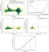 |
Fig. B.1. Top left: Density plot of the H line-depth against line-width as identified by linefinder for all sources within 500 pc with Gaia DR3 XP spectra available. Dashed red lines indicate the thresholds in line-width and line-depth used to filter non-real H emitters (see Appendix B). Sources with widthlf > 25 nm are mostly M-dwarf contaminants. Sources with depthlf < 10−17 W/nm/m2 have emission comparable to the linefinder uncertainties. Top right: ‘accuracy’, ‘completeness’, ‘F1-score’, and ‘Fβ-score’ metrics as a function of pEW threshold for selecting H emitters. Vertical lines indicate the main thresholds used in this work (pEW < − 0.5, and < − 1.0 nm). Middle panels: Density plots of the H line-depth against line-width as identified by linefinder for all sources within 500 pc with Gaia DR3 XP spectra available and pEW < − 0.5 nm (left) or pEW < − 1.0 nm (right). Bottom panel: Plot of the fraction of contaminants against pEW threshold applied, where the number of contaminants is defined as the number of sources with with widthlf > 25 nm. |
Appendix C: Correlation between Fcont and RP
Fig. C.1 shows the correlation between Fcont and RP for the three different extinction regimes discussed in Sect. 2.4.
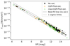 |
Fig. C.1. Correlation between the continuum flux density at the H line (Fcont) and the mean magnitude in the integrated Gaia RP band, for a sample of YSOs for which Fcont was calculated from the XP spectra. The points show all three extinction regimes discussed in Sect. 2.4. The line of best linear fit, with its uncertainties, is only shown for the case of no extinction correction. The values of the fit parameters for all three cases are presented in Table 1. |
Appendix D: YSO region on colour-magnitude diagram
To remove non-YSOs from the catalogue of Table 2, we apply a selection criterion based on the Gaia colour-magnitude diagram (BP-RP vs absolute G magnitude). We convert the G band mean magnitude to absolute magnitude using the geometric distances of Bailer-Jones et al. (2021). As the goal is to perform a filtering of obvious non-YSO objects, we focus on highlighting the regions clearly incompatible with YSOs in the CMD (by adding generous margins to the Baraffe et al. 2015 tracks). In particular, we select as YSO-compatible the sources that fall in the area bounded by the following lines (Fig. 3):
 (D.1)
(D.1)
This CMD cut excludes populations such as white dwarfs, cataclysmic variables, evolved stars, and Classical Be stars. Sources within the YSO-compatible region are flagged in Table 2 as ‘flag_CMD’.
Appendix E: Addressing the inhomogeneous sky distribution of sources with no XP spectra
The sky distribution of sources that have no XP spectra in Gaia DR3, but that have pEW measurements available in the astrophysical_parameters table, is affected by the Gaia scanning law. Gaia scans some regions of the sky less frequently than others (Gaia Collaboration 2016), and XP spectra was not published in DR3 for sources that have fewer than 15 CCD transits contributing to the generation of the BP and RP spectra (De Angeli et al. 2023). However, pEWs were published for these sources regardless of them not having public XP spectra. We thus need to account for the fact that some entire regions of the sky have no XP spectra, and hence there is no possible removal of M-dwarf contaminants via linefinder (see Sect. 2.6 and Appendix B). The obvious approach of not considering pEWs for sources with no XP spectra is not adequate. This is because, importantly, most known YSOs have no public XP spectra due to unrelated internal reasons (private communication with Gaia helpdesk), but they also have pEW measurements in DR3.
To evaluate this artificial higher-fraction of contaminants in Table 2 in certain regions of the sky, we projected the sources with no XP spectra in the sky and manually selected the regions with no public XP spectra because of the Gaia scanning law. Sources in the selected regions are flagged in Table 2 in the column ‘flag_Gaia_scanning’. In selection criterion B (Sect. 2.7), we keep all sources that are not in these regions, and from the sources that are in these regions we only keep the strongest accretors, defined as the sources with log(Lacc,med-GSP-Phot extinction/L⊙) > − 3.5. This number was chosen so the density of YSO H emitters in the regions with poor Gaia coverage matches the density of YSO H emitters in nearby regions with good Gaia coverage. Fig. E.1 shows the inhomogeneous distribution of sources with no XP spectra and the regions that we selected as affected by the Gaia scanning law. More information on how to evaluate and work with the Gaia scanning law can be found in Cantat-Gaudin et al. (2023) and Castro-Ginard et al. (2023).
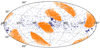 |
Fig. E.1. All sources from Gaia DR3 within 500 pc with pEW < − 0.5 nm but with no XP spectra publicly available. The Gaia scanning law footprint is clearly visible. We colour-code in orange the sources that have no XP spectra because of poor Gaia coverage. The sources in blue do not have XP spectra because of other reasons. Of the sources in orange, we only consider in criterion B (Sect. 2.7) the ones with log(Lacc,med-GSP-Phot extinction/L⊙) > − 3.5. |
Appendix F: Plots of accretion properties versus stellar parameters in Sco-Cen
Fig F.1 shows the fits used to derive the slopes of Fig. 15 for ten different Sco-Cen clusters. All fits were performed using using the Bayesian method of Kelly (2007) to propagate errors.
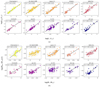 |
Fig. F.1. Plots of the fits used to derive the slopes of Fig. 15. Each is the fit is of a specific cluster of Sco-Cen, and the colours match those used in Fig. 15. The value of the slope of each region is reported. Fig. (a): log Lacc vs log L⋆; Fig. (b): log Ṁacc vs log M⋆. |
All Tables
Parameters derived in this work from Gaia XP spectra and pEW for H emitters within 500 pc (145 975 sources).
Fraction of accreting stars, median accretion luminosity, and median mass accretion rate for 34 Sco-Cen clusters.
Fit parameters for the evolution of fraction of accretors (facc), median Lacc of the accretors and median Ṁacc of the accretors in Sco-Cen clusters with age, where by accretors we mean sources with pEW < − 1.0 nm.
Fraction of accreting stars, median accretion luminosity, and median mass accretion rate for various star-forming regions and groups within 500 pc.
All Figures
|
Fig. 1. Correlation between H equivalent widths from medium-resolution spectra and Gaia H pseudo-equivalent widths, for a sample of YSOs (T Tauri and Herbig stars). The black lines represent the best linear fit to the data and its uncertainties, log(−EWHα) = (1.13 ± 0.04)⋅log(−pEW)+(0.41 ± 0.02)±0.18. |
| In the text | |
|
Fig. 2. Diagram illustrating the various selections applied to the original sample of all Gaia DR3 sources within 500 pc with measured pEW to obtain the final sample of YSO candidates (Table 2), and the different quality flags that can be applied to further refine the purity of the sample. The two boxes on the right show two of the steps in more detail. |
| In the text | |
|
Fig. 3. Colour-magnitude diagram (CMD) of all H emitter candidates within 500 pc (Table 2). The 1494 sources outside of the red lines are flagged in Sect. 2.7 as being incompatible with a YSO location in the CMD. The equations to reproduce the lines are reported in Appendix D. The sources are colour-coded by accretion luminosity, using the accretion luminosity calculated using med-GSP-Phot extinction. Grey sources belong to the 1% of the sample which does not have med-GSP-Phot extinction. |
| In the text | |
|
Fig. 4. Colour-colour plot using 2MASS and WISE magnitudes. The sources in the plot were pre-selected using the colour-magnitude diagram of Fig. 3, and by excluding upper limits. The region to the top right (J − Ks > 0.60 mag and W1 − W2 > 0.25 mag) is the region considered when applying selection criterion A (Sect. 2.7). The sources are colour-coded by accretion luminosity, using the accretion luminosity calculated using med-GSP-Phot extinction. Grey sources belong to the 1% of the sample which does not have med-GSP-Phot extinction. |
| In the text | |
|
Fig. 5. Accretion luminosity divided by stellar luminosity as a function of effective temperature for the all-sky YSOs with accretion luminosity and effective temperature calculated from med-GSP-Phot extinction, from samples A (flag_IR, 4086 sources), B (flag_pEW, 5934 sources), and C (flag_combined, 1871 sources). All sources from sample C are, by definition, also included in sample A and B. Dashed lines trace the locus of chromospheric emission lines when they are erroneously converted into accretion luminosities, as derived in Manara et al. (2017a). 8.44% of sample A and 0.15% of sample B are below the chromospheric emission lines. |
| In the text | |
|
Fig. 6. Fig. (a): Sky plot in galactic co-ordinates of YSO H emitters selected using criterion A (filtering by IR excess, Sect. 2.7). Fig. (b): Sky plot in galactic co-ordinates of YSO H emitters selected using criterion B (filtering by pEW). Fig. (c): Sky plot in galactic co-ordinates of YSO H emitters selected using criterion C, which is the intersection of sources in A and B. In Fig. (c), the plot is zoomed in around the Galactic plane. The star-forming regions are labelled following Avedisova (2002). The sources are colour-coded by their accretion luminosity calculated using med-GSP-Phot extinction (Sect. 2.4). The few sources without med-GSP-Phot extinction are shown in grey. |
| In the text | |
|
Fig. 7. Histogram of distances of YSO H emitter candidates including the full table with ‘flag_CMD’ and samples A, B, and C (these being refined subsets of YSO candidates, Sect. 2.7). We use the geometric distances of Bailer-Jones et al. (2021). |
| In the text | |
|
Fig. 8. Detail of some star-forming regions from Fig. 6 bottom panel (sample C), plotted over the Planck map at 217 GHz (Planck Collaboration III 2020). YSOs with higher accretion luminosities can be appreciated concentrated in the more clustered areas, following the structure of the regions. |
| In the text | |
|
Fig. 9. Comparison of the accretion luminosities and mass accretion rates of this work with the values reported in Manara et al. (2023) from higher-resolution spectroscopy. The dashed black lines are the 1:1 lines, and the dashed grey lines show ±1 dex. Top panels: Three plots showing accretion luminosities calculated without accounting for extinction (left), using Gaia GSP-Phot extinction (central), and using med-GSP-Phot extinction (right). Bottom panels: Two plots showing mass accretion rates calculated using Gaia GSP-Phot extinction (left), and using med-GSP-Phot extinction (right). |
| In the text | |
|
Fig. 10. Distribution of accretion luminosities and mass accretion rates derived for YSO H emitters within 500 pc. Different lines trace the quality filters described in Sect. 2.7 (see Fig. 2). The left panels present accretion properties obtained using the GSP-Phot extinction correction and the right panels the ones obtained using the med-GSP-Phot extinction correction (Sect. 2.4). We have added to this plot the accretion luminosities and mass accretion rates presented in Manara et al. (2023) for well-characterised T Tauri stars from higher-resolution spectroscopy. The central panels are cumulative distributions of the accretion properties shown on left panels, using GSP-Phot extinction. |
| In the text | |
|
Fig. 11. Left: Accretion luminosity vs. stellar luminosity for 1871 YSOs all-sky within 500 pc (sample C, Sect. 2.7). The 655 sources of the sample that have GSP-Phot extinction are plotted according to their values of accretion luminosity and stellar luminosity derived using this extinction. The black line is the fit for the GSP-Phot values of these 656 sources. The value of the slope in the log-log plane is 1.41 ± 0.02. The remaining sources of sample C that do not have GSP-Phot extinction are plotted using the values calculated using med-GSP-Phot. The results of fitting to values calculated with med-GSP-Phot are reported in Table 3. Right: Mass accretion rate vs. stellar mass for the same sample of 1871 YSOs. The 656 sources of the sample that have GSP-Phot extinction are plotted according to their values derived using this extinction. The black line is the fit to the GSP-Phot values, for sources with stellar mass M⋆ < 1.0 M⊙, and with Ṁacc > 10−12 M⊙/yr. The value of the slope in the log-log plane is 2.4 ± 0.1. Again, the sources of sample C that do not have GSP-Phot extinction are plotted using the values calculated using med-GSP-Phot. |
| In the text | |
|
Fig. 12. Three-dimensional spatial distribution of 1954 members of the 34 Sco-Cen clusters identified by Ratzenböck et al. (2023a), colour-coded by accretion luminosity. The co-ordinates are provided in Ratzenböck et al. (2023a) and are such that the Sun is at (0,0,0) and the Z = 0 plane is parallel to the Galactic plane. For better visualisation, see the interactive 3D version online. |
| In the text | |
|
Fig. 13. Evolution of accretion in Sco-Cen clusters with age. Each point represents one of the 34 Sco-Cen clusters whose ages were calculated in Ratzenböck et al. (2023b). The ages shown here are the Baraffe et al. (2015) Bp-Rp ages of that work. In each panel, we show two fits: an exponential decay (Eq. (7)) and a power law (Eq. (8)). Top panel: we show the percentage of YSO accretors per cluster facc. The accretion timescale obtained from fitting the exponential is τacc = 2.7 ± 0.4 Myr. Bottom two panels: median accretion luminosity and the median mass accretion rate of the accretors (sources with pEW < − 1.0 nm) in each cluster. Only the cluster members with stellar mass in the range 0.08 < M⋆ < 0.25 M⊙ were considered for the medians, to remove dependencies with stellar mass. Only clusters with four or more accretors in this mass range were considered. All fit parameters are reported in Table 5. |
| In the text | |
|
Fig. 14. Stellar mass distribution of accretors in the Sco-Cen clusters vs. cluster age (Baraffe et al. 2015-BpRp). The plot shows the stellar masses of all cluster members with pEW < − 1.0 nm as derived in Sect. 2.5 (Table 2), and the cluster median both before (orange) and after (blue) applying the 0.06 < M⋆ < 0.22 M⊙ cut (red lines). The median mass is only shown if there are at least four cluster members in the chosen mass range. We note this filtering by stellar mass results in similar median stellar masses for all clusters. |
| In the text | |
|
Fig. 15. Slope of the correlations of accretion luminosity vs. stellar luminosity (top panel), and mass accretion rate vs. stellar mass (bottom panel) for ten clusters of Sco-Cen, plotted against cluster age (Baraffe et al. 2015 Bp-Rp ages). For each cluster, we measured the slope of the correlations in the logarithmic plane, using values calculated with med-GSP-Phot, and only considering sources with pEW < − 1.0 nm. Only clusters where at least 20 sources could be used in the fit were considered. Each point is colour-coded to match the corresponding fit in Appendix F. |
| In the text | |
|
Fig. 16. Fraction of accretors against age for each region of Table 6, over-plotted on the top panel of Fig. 13. The Table 6 regions (orange stars in the plot) are labelled. The blue dots are the Sco-Cen clusters of Fig. 13 and the red and green line are, respectively, the power law and exponential fit to the Sco-Cen clusters, obtained in Sect. 4.1. |
| In the text | |
|
Fig. B.1. Top left: Density plot of the H line-depth against line-width as identified by linefinder for all sources within 500 pc with Gaia DR3 XP spectra available. Dashed red lines indicate the thresholds in line-width and line-depth used to filter non-real H emitters (see Appendix B). Sources with widthlf > 25 nm are mostly M-dwarf contaminants. Sources with depthlf < 10−17 W/nm/m2 have emission comparable to the linefinder uncertainties. Top right: ‘accuracy’, ‘completeness’, ‘F1-score’, and ‘Fβ-score’ metrics as a function of pEW threshold for selecting H emitters. Vertical lines indicate the main thresholds used in this work (pEW < − 0.5, and < − 1.0 nm). Middle panels: Density plots of the H line-depth against line-width as identified by linefinder for all sources within 500 pc with Gaia DR3 XP spectra available and pEW < − 0.5 nm (left) or pEW < − 1.0 nm (right). Bottom panel: Plot of the fraction of contaminants against pEW threshold applied, where the number of contaminants is defined as the number of sources with with widthlf > 25 nm. |
| In the text | |
|
Fig. C.1. Correlation between the continuum flux density at the H line (Fcont) and the mean magnitude in the integrated Gaia RP band, for a sample of YSOs for which Fcont was calculated from the XP spectra. The points show all three extinction regimes discussed in Sect. 2.4. The line of best linear fit, with its uncertainties, is only shown for the case of no extinction correction. The values of the fit parameters for all three cases are presented in Table 1. |
| In the text | |
|
Fig. E.1. All sources from Gaia DR3 within 500 pc with pEW < − 0.5 nm but with no XP spectra publicly available. The Gaia scanning law footprint is clearly visible. We colour-code in orange the sources that have no XP spectra because of poor Gaia coverage. The sources in blue do not have XP spectra because of other reasons. Of the sources in orange, we only consider in criterion B (Sect. 2.7) the ones with log(Lacc,med-GSP-Phot extinction/L⊙) > − 3.5. |
| In the text | |
|
Fig. F.1. Plots of the fits used to derive the slopes of Fig. 15. Each is the fit is of a specific cluster of Sco-Cen, and the colours match those used in Fig. 15. The value of the slope of each region is reported. Fig. (a): log Lacc vs log L⋆; Fig. (b): log Ṁacc vs log M⋆. |
| In the text | |
Current usage metrics show cumulative count of Article Views (full-text article views including HTML views, PDF and ePub downloads, according to the available data) and Abstracts Views on Vision4Press platform.
Data correspond to usage on the plateform after 2015. The current usage metrics is available 48-96 hours after online publication and is updated daily on week days.
Initial download of the metrics may take a while.