| Issue |
A&A
Volume 699, July 2025
|
|
|---|---|---|
| Article Number | A34 | |
| Number of page(s) | 26 | |
| Section | Interstellar and circumstellar matter | |
| DOI | https://doi.org/10.1051/0004-6361/202452700 | |
| Published online | 27 June 2025 | |
ALMAGAL
IV. Morphological comparison of molecular and thermal dust emission using the histogram of oriented gradients method
1
INAF-Istituto di Astrofisica e Planetologia Spaziale,
Via Fosso del Cavaliere 100,
00133
Roma,
Italy
2
Institut de Ciències de l’Espai (ICE), CSIC, Campus UAB, Carrer de Can Magrans s/n,
08193
Bellaterra (Barcelona),
Spain
3
Institut d’Estudis Espacials de Catalunya (IEEC),
08860,
Castelldefels (Barcelona),
Spain
4
Dipartimento di Fisica, Sapienza Università di Roma,
Piazzale Aldo Moro 2,
00185
Rome,
Italy
5
Dipartimento di Fisica, Università di Roma Tor Vergata,
Via della Ricerca Scientifica 1,
00133
Roma,
Italy
6
I. Physikalisches Institut, Universität zu Köln,
Zülpicher Str. 77,
50937
Köln,
Germany
7
University of Connecticut, Department of Physics,
2152 Hillside Road, Unit 3046 Storrs,
CT
06269,
USA
8
Institute of Astronomy and Astrophysics, Academia Sinica,
11F of ASMAB, AS/NTU No. 1, Sec. 4, Roosevelt Road,
Taipei
10617,
Taiwan
9
East Asian Observatory,
660 N. A’ohoku, Hilo,
Hawaii,
HI
96720,
USA
10
INAF-Osservatorio Astrofisico di Arcetri,
Largo E. Fermi 5,
50125
Firenze,
Italy
11
Max Planck Institute for Astronomy,
Königstuhl 17,
69117
Heidelberg,
Germany
12
Jodrell Bank Centre for Astrophysics,
Oxford Road, The University of Manchester,
Manchester
M13 9PL,
UK
13
Universität Heidelberg, Zentrum für Astronomie, Institut für Theoretische Astrophysik,
Heidelberg,
Germany
14
Universität Heidelberg, Interdisziplinäres Zentrum für Wissenschaftliches Rechnen,
Heidelberg,
Germany
15
Center for Astrophysics | Harvard & Smithsonian,
60 Garden St,
Cambridge,
MA
02138,
USA
16
Elizabeth S. and Richard M. Cashin Fellow at the Radcliffe Institute for Advanced Studies at Harvard University,
10 Garden Street,
Cambridge,
MA
02138,
USA
17
Center for Data and Simulation Science, University of Cologne,
Germany
18
ASTRON, Netherlands Institute for Radio Astronomy,
Oude Hoogeveensedijk 4,
Dwingeloo,
7991
PD,
The Netherlands
19
Dipartimento di Fisica e Astronomia, Università degli Studi di Firenze,
Via G. Sansone 1,
50019
Sesto Fiorentino, Firenze,
Italy
20
SKA Observatory, Jodrell Bank, Lower Withington,
Macclesfield
SK11 9FT,
UK
21
UK ALMA Regional Centre Node,
M13 9PL,
UK
22
National Radio Astronomy Observatory,
520 Edgemont Road,
Charlottesville,
VA
22903,
USA
23
Max-Planck-Institute for Extraterrestrial Physics (MPE),
Garching bei München,
Germany
24
Laboratory for the study of the Universe and eXtreme phenomena (LUX), Observatoire de Paris,
Meudon,
France
25
Université Paris-Saclay, Université Paris-Cité, CEA, CNRS, AIM,
91191
Gif-sur-Yvette,
France
26
School of Engineering and Physical Sciences, Isaac Newton Building, University of Lincoln, Brayford Pool,
Lincoln
LN6 7TS,
UK
27
Faculty of Physics, University of Duisburg-Essen,
Lotharstraße 1,
47057
Duisburg,
Germany
28
Jet Propulsion Laboratory, California Institute of Technology,
4800 Oak Grove Drive,
Pasadena,
CA
91109,
USA
29
Shanghai Astronomical Observatory, Chinese Academy of Sciences,
Shanghai
200030,
PR
China
30
School of Physics and Astronomy, University of Leeds,
Leeds
LS2 9JT,
UK
31
INAF-Istituto di Radioastronomia & Italian ALMA Regional Centre,
Via P. Gobetti 101,
40129
Bologna,
Italy
32
Department of Astronomy, School of Science, The University of Tokyo,
7-3-1 Hongo, Bunkyo,
Tokyo
113-0033,
Japan
33
Department of Earth and Planetary Sciences, Institute of Science Tokyo, Meguro,
Tokyo
152-8551,
Japan
34
National Astronomical Observatory of Japan, National Institutes of Natural Sciences,
2-21-1 Osawa, Mitaka,
Tokyo
181-8588,
Japan
35
Dipartimento di Fisica e Astronomia, Alma Mater Studiorum – Università di Bologna,
Bologna,
Italy
36
SRON Netherlands Institute for Space Research,
Landleven 12,
9747
AD
Groningen,
The Netherlands
37
Kapteyn Astronomical Institute, University of Groningen,
The Netherlands
38
Departamento de Astronomía, Universidad de Chile,
Casilla 36-D,
Santiago,
Chile
39
Zhejiang Laboratory,
Hangzhou
311100,
PR
China
40
Universidad Autonoma de Chile,
Pedro de Valdivia 425,
9120000
Santiago de Chile,
Chile
★ Corresponding author: This email address is being protected from spambots. You need JavaScript enabled to view it.
Received:
22
October
2024
Accepted:
10
April
2025
Abstract
Context. The study of molecular line emission is crucial to unveil the kinematics and the physical conditions of gas in star-forming regions. We use data from the ALMAGAL survey, which provides an unprecedentedly large statistical sample of high-mass star-forming clumps that helps us to remove bias and reduce noise (e.g., due to source peculiarities, selection, or environmental effects) to determine how well individual molecular species trace continuum emission.
Aims. Our aim is to quantify whether individual molecular transitions can be used reliably to derive the physical properties of the bulk of the H2 gas, by considering morphological correlations in their overall integrated molecular line emission with the cold dust. We selected transitions of H2CO, CH3OH, DCN, HC3N, CH3CN, CH3OCHO, SO, and SiO and compared them with the 1.38 mm dust continuum emission at different spatial scales in the ALMAGAL sample. We included two transitions of H2CO to understand whether the validity of the results depends on the excitation condition of the selected transition of a molecular species. The ALMAGAL project observed more than 1000 candidate high-mass star-forming clumps in ALMA band 6 at a spatial resolution down to 1000 au. We analyzed a total of 1013 targets that cover all evolutionary stages of the high-mass star formation process and different conditions of clump fragmentation.
Methods. For the first time, we used the method called histogram of oriented gradients (HOG) as implemented in the tool astroHOG on a large statistical sample to compare the morphology of integrated line emission with maps of the 1.38 mm dust continuum emission. For each clump, we defined two masks: the first mask covered the extended more diffuse continuum emission, and the second smaller mask that only contained the compact sources. We selected these two masks to study whether and how the correlation among the selected molecules changes with the spatial scale of the emission, from extended more diffuse gas in the clumps to denser gas in compact fragments (cores). Moreover, we calculated the Spearman correlation coefficient and compared it with our astroHOG results.
Results. Only H2CO, CH3OH, and SO of the molecular species we analyzed show emission on spatial scales that are comparable with the diffuse 1.38 mm dust continuum emission. However, according the HOG method, the median correlation of the emission of each of these species with the continuum is only ~24–29%. In comparison with the dusty dense fragments, these molecular species still have low correlation values that are below 45% on average. The weak morphological correlation suggests that these molecular lines likely trace the clump medium or outer layers around dense fragments on average (in some cases, this might be due to optical depth effects) or also trace the inner parts of outflows at this scale. On the other hand DCN, HC3N, CH3CN3 and CH3OCHO are well correlated with the dense dust fragments at above 60%. The lowest correlation is seen with SiO for the extended continuum emission and for compact sources. Moreover, unlike other outflow tracers, in a large fraction of the sources, SiO does not cover the area of the extended continuum emission well. This and the results of the astroHOG analysis reveal that SiO and SO do not trace the same gas, in contrast to what was previously thought. From the comparison of the results of the HOG method and the Spearman correlation coefficient, the HOG method gives much more reliable results than the intensity-based coefficient when the level of similarity of the emission morphology is estimated.
Key words: astrochemistry / molecular data / ISM: general / ISM: lines and bands / ISM: molecules
© The Authors 2025
 Open Access article, published by EDP Sciences, under the terms of the Creative Commons Attribution License (https://creativecommons.org/licenses/by/4.0), which permits unrestricted use, distribution, and reproduction in any medium, provided the original work is properly cited.
This article is published in open access under the Subscribe to Open model. This email address is being protected from spambots. You need JavaScript enabled to view it. to support open access publication.
1 Introduction
The study of molecular line emission in star-forming regions is extremely important not only for understanding the chemical content of the environment in which stars form, but also for constraining the physical and dynamic properties of the gas (e.g., Kennicutt & Evans 2012; Beuther et al. 2006; Beltrán et al. 2018). Based on the analysis of the line emission, it is possible to infer the average velocity and velocity dispersion of the emitting gas, and also its column density and temperature, when we detect multiple transitions of the same molecular species. Moreover, the combined analysis of several molecular species can help us to constrain quantities such as the column density of H2, the volume density, and the UV radiation field (Gratier et al. 2017). It is known that different molecular species can trace different regions in the star formation scenario (e.g., van Dishoeck & Blake 1998; Caselli & Ceccarelli 2012; Tychoniec et al. 2021), depending on the physical conditions required for the production and release of each molecular species in the gas phase. In addition, different transitions of a molecular species can be excited and emit in gas with higher/lower temperatures and densities. The use of various tracers in star-forming regions arises because the main component of the interstellar medium (ISM), that is, the hydrogen molecule (H2), has no permanent dipole moment and has the lowest moment of inertia of all the molecular species. As a result, there are no allowed transitions of H2 that can be excited under typical conditions in cold and dense of star-forming regions (Stahler & Palla 2004). Therefore, an indirect method for tracing H2 in star-forming regions on scales below 1 pc, where the CO emission (the typical proxy of H2) is usually optically thick (Kennicutt & Evans 2012), is to use the dust continuum emission at millimeter wavelengths, assuming a constant ratio of the density of the H2 and the dust density. Much of the crucial information that is contained in the line emission, such as the kinematics of the material, cannot be obtained from dust emission, however. Therefore, studying how well individual molecular species trace the continuum emission is crucial for assessing whether the estimates made from the analysis of these species in the bulk of the gas emission under different conditions are reliable.
In this framework, we analyze the molecular line emission in star-forming regions in the dataset of the ALMA Evolutionary study of High Mass Protocluster Formation in the Galaxy (ALMAGAL), which is the largest sample of star-forming regions ever observed at a high spatial resolution with the Atacama Large Millimeter/Submillimeter Array (ALMA). ALMAGAL is an ALMA large project (2019.1.00195.L; PIs: Molinari, Schilke, Battersby, Ho; Molinari et al. 2025; Sánchez-Monge et al. 2025) that targeted more than 1000 candidate high-mass star-forming regions with a resolution of ~1000 au that covered all the evolutionary stages of the star formation process and different environmental conditions (from the tip of the bar to the outer galaxy) and showed different fragmentation properties (Coletta et al. 2025, Elia et al., in prep.). This provides a robust statistical basis for our study.
We analyzed the emission morphology of eight commonly detected molecular tracers of star-forming regions (H2CO, CH3OH, DCN, HC3N, CH3CN, CH3OCHO, SO, and SiO) in the 1.38 mm band (ALMA band 6) and compared it to the dust continuum emission on different spatial scales.
To study the morphological correlation of emission from selected molecular species with the dust continuum emission we use the method of the histogram of oriented gradients (HOG) (Soler et al. 2019). The HOG method uses the orientation of the spatial gradients of different images (or 3D data cubes) to compare their emission morphology. Previous applications of the HOG method included the pairing of atomic and molecular emission toward molecular clouds in the Galactic plane (Syed et al. 2020), the correlation between neutral atomic hydrogen (HI) emission and Faraday synthesis cubes (Bracco et al. 2020), the characterization of the line emission from molecular species in three high-mass star formation regions (Liu et al. 2020; Gieser et al. 2022), and the comparison between the 3D reconstruction of the interstellar dust density and the HI and carbon monoxide (CO) emission (Soler et al. 2023). Studies of the correlation between the emission in high-resolution observations of high-mass star-forming regions were mostly carried out using intensity-based statistical correlators, such as the cross-correlation, the Pearson coefficient, or the Spearman coefficient, to study the correlation between different molecular species (e.g., Guzmán et al. 2018; Li et al. 2022).
We present a more sophisticated approach for the first time for a sample of this size that compares the total morphology of the emission and not only the intensity pixel by pixel, as was usually done so far. In particular, we compare the morphology of the integrated-intensity maps of several molecular species with the morphology of the continuum emission from the cold dust in the largest sample of star-forming regions using the HOG method.
This paper is organized as follows. In Section 2, we present the ALMAGAL sample and the molecular species we analyzed. In Section 3, we describe the observations and the data reduction process. In Section 4, we describe the derivation of the integrated line-intensity maps (moment-0 maps) and the tool used to investigate the morphological correlation of the molecular species with the dust continuum emission: astroHOG. Section 5 presents a discussion of the results, where we show emission in the same regions of the maps does not imply that the emission morphology is well correlated for all the species, and we demonstrate the importance of using a dedicated tool for studying the morphology. Finally, we present our conclusions in Section 6.
2 Sources and molecule selection
2.1 The sample
The ALMAGAL sample includes 1017 high-mass clumps with masses M> 500 M⊙, surface densities Σ> 0.1 g cm−2, located at heliocentric distances up to 7.5 kpc, and covering evolutionary stages from starless clumps to HII regions. Due to the close proximity (below the FOV size) of three pairs of sources and the exclusion of Eta Carinae, the sample analyzed is of 1013 sources (see Molinari et al. 2025 for further details). The sample spans four orders of magnitude in the luminosity-to-mass ratio (L/M), a distance-independent indicator of the evolutionary stage of a star-forming region (Molinari et al. 2008, 2016, 2019; Giannetti et al. 2017; Elia et al. 2017, 2021; König et al. 2017). During the first stages of star formation, L/M increases due to the increase of the accretion rate with time and therefore accretion luminosity, while the central object is still very embedded in its envelope so that the total mass M does not vary significantly.
Using this parameter, it is possible to roughly divide starless sources, having L/M < 1 L⊙/M⊙, from protostellar objects, with 1 < L/M < 10 L⊙/M⊙, and from candidate ultra-compact HII (UC HIIs) regions, with L/M > 10 L⊙/M⊙ (Cesaroni et al. 2015; Elia et al. 2017; Elia 2020; Elia et al. 2021).
Within the ALMAGAL sample, the clump masses are in the range between 102 M⊙ and 104 M⊙, and the number of fragments varies from one up to 50, with a median value over the whole sample of five (Coletta et al. 2025). We give an overview of the properties of the ALMAGAL sample in Figure 1, where the pink histogram highlights the properties of a subsample of sources for which the automated routine for the creation of moment-0 maps failed (see Section 4.1). For these sources, moment-0 maps have been created integrating over a fixed velocity range.
The ALMAGAL survey and its dataset have already been described by Molinari et al. (2025) and Sánchez-Monge et al. (2025), including a description of the reduction pipeline and full characterization of the clumps. Moreover, Coletta et al. (2025) performed a detailed study of the fragmentation properties in each clump, and Wells et al. (2024) studied the accretion flows of gas from the lines of H2CO in a sub-sample of ALMAGAL sources.
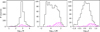 |
Fig. 1 Physical properties of the clumps in the ALMAGAL sample (shown in black). The subsample for which we created moment-0 maps using a fixed velocity range of ±5 km/s around the clump systemic velocity (see Section 4.1) is shown in magenta with shading. From left to right: mass of the clumps M in units of M⊙, the L/M ratio of the clumps in units of L⊙/M⊙, and the surface density of the clumps Σ in units of g/cm2. |
Summary of the molecular emission lines.
2.2 Molecular transitions
We analyzed the emission morphology of eight commonly detected molecular tracers of star-forming regions (H2CO, CH3OH, DCN, HC3N, CH3CN, CH3OCHO, SO, and SiO; the selected transitions are listed in Table 1) in the 1.38 mm band (ALMA Band 6) and compared it to the dust continuum emission on different spatial scales. To investigate the dependence of the results on the selected transition for each molecular species, and on the upper level energy and critical density, we selected two of the three available transitions for H2CO, which is expected to be the most commonly detected molecule in the sample.
The species selected include both simple and complex molecules (i.e., molecules made of six or more atoms) as well as well-known shock tracers such as SiO and SO. Even though we expect the emission of those molecular species to not correlate with the extended dust continuum emission, we do not know how those molecular species correlate with continuum emission at cores scale, and with this study we will be able to quantify it. This is especially true for SO, since other studies have underlined that SO can also trace a hot envelope around protostellar sources (e.g., Tychoniec et al. 2021). The spectral setup of ALMAGAL includes also lines of 13CO and C18O. However, we excluded from the analysis these two tracers since in most cases their emission covers the entire FOV of the observations, and extend even further, unlike all other species analyzed in this paper, which raises problems in the cleaning of those spectral channel, leading to possible artefacts and filtering.
In the following paragraphs we give a brief review of the main formation pathways for all the molecular species analyzed in the paper.
H2CO forms on grains from hydrogenation of CO (Charnley et al. 1997; Watanabe et al. 2004; Garrod et al. 2008), and is released in gas phase when the temperature raises above 40 K (Garrod et al. 2008), but also through gas-phase reactions (Le Teuff et al. 2000; Garrod & Herbst 2006; Fuchs et al. 2009; Chacón-Tanarro et al. 2019). Methanol is quite exclusively formed on dust-grains, mainly from the hydrogenation of CO, after the formation of H2CO (Charnley et al. 1997; Watanabe et al. 2004; CO → HCO → H2CO → CH2CO, CH3O → CH3OH), or through a secondary route by CH3OH+H2CO → CH3OH + HCO, on dust grains (Simons et al. 2020; Santos et al. 2022). It is then released in gas phase mainly due to thermal desorption from T~150 K (Luna et al. 2017), but non-thermal desorption mechanisms are at play to explain its detection in cold environment. These two molecules can also be released due to grain-sputtering and therefore probe outflows, as their emission shows high-velocity wings and their column densities have been found to be well correlated with the one of SiO (Li et al. 2022). Indeed, also in our ALMAGAL sample, we found evidence of contribution from outflowing gas in the emission of these two molecular species.
HCCCN can form through gas phase reactions starting mainly from the release in gas-phase of CH4 above 25 K, which reacts with C+ to form C2H2, followed by C2H2+CN→HCCCN+H, and increase its production at T>55 K when also C2H2 thermally desorb from dust grains (Hassel et al. 2008). However, the HCCCN formed in gas-phase is partly depleted onto dust-grains, and the highest abundances are reached when it desorb at T above ~90 K (Taniguchi et al. 2019). Therefore it is expected to be detected only in the more warm regions.
The main pathway of formation for CH3CN is on the surface of dust grains from the reactions of CH3 with CN (Garrod et al. 2008). Another grain surface pathways for its formation is the multiple hydrogenation of C2N, and modest abundances of this molecules are also produced in gas-phase following the desorption of HCN from the grains (Garrod et al. 2008).
CH3OCHO formation is mainly the result of the reactions of HCO and CH3OH on grains. This reaction can occur already at T~10 K, but higher temperature around 20–40 K increase the methyl formate production thanks to the higher mobility of the reactants. The majority of CH3OCHO is released in gas-phase at temperature above 100 K (Burke et al. 2015), so also this line is expected in the hot regions around protostars.
The reactions that leads to the formation of DCN are gas-phase reactions, with both cold and warm/high temperature reactions. However, unlike other deuterated species, the predominant part of the production of DCN takes place in warm gas up to and even above 70 K (Millar et al. 1989; Turner 2001; Roueff et al. 2007; Albertsson et al. 2013).
SiO is a well known shock tracer and its abundance is enhanced up to six order of magnitudes in outflow regions (Martin-Pintado et al. 1992). In those regions grain sputtering releases in gas-phase a significant amount of atomic Si or Si-bearing molecules, which leads to the formation of SiO (Schilke et al. 1997; Jiménez-Serra et al. 2008). However, a narrow SiO emission has been observed, which might be due to low-velocity shocks, or cloud-cloud collisions (Jiménez-Serra et al. 2008; Louvet et al. 2016; Cosentino et al. 2022; Duarte-Cabral et al. 2014). Lastly, S atoms freeze on dust grains during the cold collapse phase, where H2S is mainly formed. After its release in gas phase at high temperature (T>100 K) rapid hot gas-phase reactions lead to the formation of SO (Charnley et al. 1997; Wakelam et al. 2004, 2011). However, Esplugues et al. (2013) observed an increase of three orders of magnitude in SO abundances in regions affected by shocks, and Fontani et al. (2023) observed that SO can trace both quiescient and turbulent material depending on the source, thus the sputtering of dust grains is likely increasing the SO formation in outflow regions, as in the case of SiO.
3 Observations and data reduction
The ALMAGAL program (project code: 2019.1.00195.L in Cycle 7) was observed between October 2019 and July 2022. To achieve the requested linear resolution of ~1000 au without losing information on diffuse material at the clump scale, each target was observed with the 7-m array (hereafter 7M) and with two configurations of the main ALMA array. To resolve almost the same spatial scale of about 1000 au for all the sources that are at different distances, the sample was divided in two bins of distance. The near sources (i.e., sources with d < 4.7 kpc) were observed in configurations C-2 and C-5 of the main array, while the far sources (i.e., sources with d > 4.7 kpc) were observed in configurations C-3 and C-6. Using the standard pipeline, we calibrated the data of the single arrays (hereafter 7M; TM2, C-2 and C-3, intermediate resolution configuration of the main array; TM1, C-5 and C-6, highest resolution configuration of the main array). The ALMAGAL team developed a dedicated pipeline to obtain the final cubes using joint deconvolution of the various configurations observed that includes self-calibration for the most intense sources. Moreover, an iterative procedure starting from the standard ALMA-pipeline function findcont was implemented, to refine the determination of the continuum channels used to create the continuum images and the line-only cubes. A detailed description of this routine, together with a quality assessment of the final products, is presented in Sánchez-Monge et al. (2025). For the purpose of this work, we decided to analyze the cubes and continuum maps obtained by the joint deconvolution of 7M and TM2 data only (hereafter 7M+TM2), which reach a linear resolution of ~5000 au, because they recover with a better signal-to-noise ratio the diffuse emission on large scales compared to the 7M+TM2+TM1 cubes obtained from the joint deconvolution of all the available configurations that reach the aforementioned maximum resolution of ~1000 au.
The spectral setup of the observations covers four spectral windows in total: two spectral windows with a 1.9 GHz bandwidth and spectral resolution of 0.98 MHz (~1.3 km s−1) centered at 217.8 GHz and 220.0 GHz, and two higher resolution spectral windows with 0.47 GHz bandwidth and spectral resolution of 0.24 MHz (~0.3 km/s) centered at 218.3 GHz and 220.6 GHz, respectively.
4 Method
4.1 Creating the moment maps
The generation of the moment-0 maps for the sources in our sample was not feasible individually, given the large number of fields. We automated the procedure to estimate, for each molecular line in each source, the extremes of integration of the line in the velocity space, and then we created the moment-0 maps integrating the spectral cube inside that range for all the pixels. The details of this automated routine are given in Appendix B.
The CH3CN 120−110 and 121−111 lines are heavily blended in several sources. Therefore, for these two transitions, we created a single moment-0 map that includes the emission of both transitions.
All the maps for each field and transition were then visually inspected to validate them. This was done by looking at the line observed in the spectra averaged on each continuum compact source detected by the source extraction algorithm CuTEx (CUrvature Thresholding EXtractor; Molinari et al. 2011, 2016 see Sect. 4.4; following the same method as was used in Coletta et al. (2025) for 7M+TM2+TM1 data) in the clump, and checking that the velocity extremes used for the integration agree with the velocity ranges of the lines in these spectra. The employed method gives good extremes of integration, that is extremes that include the whole line for all the cores in the clump, in the majority of the sources. Two example moment 0 maps with spectra averaged over the area of each cores in the field is shown in Fig. 2, while Fig. 3 shows the moment-0 maps of all the transitions for one source. The number of sources for which the automated routine gave integration extremes that encompass all the line, without line blending problems, is 916, while for the remaining 97 sources we created the maps using a fixed velocity range. In fact, a fraction of the sample has, in at least one transition, moment-0 maps for which the extremes of integration automatically derived do not encompass the whole line or partially encompass other transitions. This is especially true for extremely line-rich sources where most lines are blended with transitions of other molecular species. For those clumps, the moment-0 maps have been recreated integrating the cube over a fixed velocity range of ±5 km/s around the systemic velocity of the clump for all the pixels. This range is a compromise between including the majority of the line, while excluding blendings in line-rich cores. These maps, in some spatial pixels, do not include the total velocity range of the line emission, since they clearly exclude possible high-velocity wings and a portion of the line if it is larger than 10 km/s.
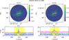 |
Fig. 2 Moment-0 maps and spectral range created with the automated routine described in Sect. 4.1. Upper row: moment-0 map of H2CO 30,3−20,2 (left) and CH3OH 22,3−31,2 (right) for source AG024.4614+0.1981. The color scales are in units of Jy/beam km/s. Lower row: spectra averaged over the 12 continuum cores detected in the source (ellipse with semiaxis the HWHM = 1.177σ from the 2D Gaussian fit). Each core spectrum has an y-axis offset to show the spectra better. The yellow area indicates the range for the velocity integration we used to obtain the moment-0 maps shown in the upper panel. The red contours are the contours of maskcom., and the white contour is the contour of maskext., defined from the continuum emission (see Section 4.4 for details). For this source, the continuum emission is shown in Fig. 4. |
4.2 Detection and mask on the moment-0 maps
To determine if a selected transition is detected in a target and to compare the emission of the different molecular species with the continuum emission, we created the masks of the line emission from the moment-0 maps. Given a moment-0 map of a selected transition of a specific field, we created a mask of all the pixels with S/N>3, excluding noise fluctuation. More details on the refinement of the moment-0 mask can be found in Appendix A. We required that at least one of the regions remaining inside the mask has a number of pixels > Nbeam, since this would be the size of emission of a point-like source. If this condition is met, we considered the transition as detected in the field.
For methyl-formate (CH3OCHO), the molecule with lowest S/N and least detected (detected in 139 sources), we visually inspected the spectra extracted towards the cores for the detected sources to confirm all the detections, since false detections could possibly alter the results on such a small sample of detections (see Section 5). We revealed only 29 false detections that were introduced into the sample where CH3OCHO was detected and we excluded these sources for the following analysis, leaving 110 sources with a real detection. This is a very small number of false detections out of the sample of 903 sources without emission of CH3OCHO (3%), and it corroborates the robustness of the automatic method applied. We expect a similar number of false detections for the other molecular species. However, these would not influence the detection statistics because they are negligible compared to the total number of detections for all the other species. Moreover, those false detections would not enter the astroHOG analysis because the regions of false emission are at the edge of the FOV and likely do not intersect with the masks defined for the continuum (see Sections 4.3 and 4.4).
4.3 Morphological analysis with astroHOG
We performed the comparison of the continuum and integrated-intensity (moment-0) maps of the molecular transitions listed in Table 1 using the HOG method presented in Soler et al. (2019). The HOG method is a machine vision tool based on the use of the intensity gradient orientation to characterize the similarities between two images. It is at the core of many algorithms used in object detection and classifications in image processing (see, for example, Leonardis et al. 2006). The implementation of the HOG method introduced by Soler et al. (2019), astroHOG1, uses tools from circular statistics to quantify the significance of the accordance of the orientation between the intensity gradients.
The basic analysis in astroHOG for two given 2D intensity maps ![Mathematical equation: $\[I_{i j}^{\mathrm{A}}\]$](/articles/aa/full_html/2025/07/aa52700-24/aa52700-24-eq1.png) and
and ![Mathematical equation: $\[I_{i j}^{\mathrm{B}}\]$](/articles/aa/full_html/2025/07/aa52700-24/aa52700-24-eq2.png) is as follows. The gradient of the two images
is as follows. The gradient of the two images ![Mathematical equation: $\[\nabla I_{i j}^{\mathrm{A}}\]$](/articles/aa/full_html/2025/07/aa52700-24/aa52700-24-eq3.png) and
and ![Mathematical equation: $\[\nabla I_{i j}^{\mathrm{B}}\]$](/articles/aa/full_html/2025/07/aa52700-24/aa52700-24-eq4.png) are calculated using Gaussian derivatives, which are the results of convolution of the images with the derivative of a Gaussian with characteristic FWHM Ω (Soler et al. 2013). This procedure is equivalent to calculating the derivative using weighted differences over points within a diameter Ω. By definition, the orientation between the gradients in a certain position ij of the maps, which is also the orientation between the iso-intensity contours, is
are calculated using Gaussian derivatives, which are the results of convolution of the images with the derivative of a Gaussian with characteristic FWHM Ω (Soler et al. 2013). This procedure is equivalent to calculating the derivative using weighted differences over points within a diameter Ω. By definition, the orientation between the gradients in a certain position ij of the maps, which is also the orientation between the iso-intensity contours, is
![Mathematical equation: $\[\phi_{i j}=\arctan \left(\frac{\left(\nabla I_{i j}^{\mathrm{A}} \times \nabla I_{i j}^{\mathrm{B}}\right) \cdot \hat{z}}{\nabla I_{i j}^{\mathrm{A}} \cdot \nabla I_{i j}^{\mathrm{B}}}\right),\]$](/articles/aa/full_html/2025/07/aa52700-24/aa52700-24-eq5.png) (1)
(1)
where ![Mathematical equation: $\[\hat{z}\]$](/articles/aa/full_html/2025/07/aa52700-24/aa52700-24-eq6.png) is the unit vector in the direction perpendicular to the plane of RA and Dec. If the two maps are identical, all of the angles ϕij are equal to 0°. If the intensity in the two maps is entirely uncorrelated, the distribution of the angles ϕij should be uniform. Thus, quantifying the similarity in the intensity distribution in the two images is related to evaluating if the distribution of angles peaks around 0°.
is the unit vector in the direction perpendicular to the plane of RA and Dec. If the two maps are identical, all of the angles ϕij are equal to 0°. If the intensity in the two maps is entirely uncorrelated, the distribution of the angles ϕij should be uniform. Thus, quantifying the similarity in the intensity distribution in the two images is related to evaluating if the distribution of angles peaks around 0°.
astroHOG tests whether the distribution of the relative orientations ϕij is uniformly distributed or has a preferential alignment at ϕ=0°, using the projected Rayleigh statistic (PRS; Durand & Greenwood 1958; Jow et al. 2018)
![Mathematical equation: $\[V=\frac{\sum_{i j} w_{i j} ~\cos~ \left(2 \phi_{\mathrm{ij}}\right)}{\left(\sum_{i j} ~w_{i j}^2 / 2\right)^{1 / 2}},\]$](/articles/aa/full_html/2025/07/aa52700-24/aa52700-24-eq7.png) (2)
(2)
where wij are the statistical weights corresponding to ϕij. Therefore, it is also independent of the intensity of the gradients, but is defined only from the relative orientations of gradients in the two maps. In our application of the method, we use the statistical weights to account for the fact that different values of ϕij inside a beam are not independent. Thus, we chose weight wij = w = δ/Δ, where δ is the size of the pixels of the image and Δ is the size of the beam of the observations. Since, in our case, the weights are the same for all the pixels, Eq. (2) becomes
![Mathematical equation: $\[V=\left(\frac{2}{N}\right)^{1 / 2} \sum_{i j} ~\cos \left(2 \phi_{\mathrm{ij}}\right).\]$](/articles/aa/full_html/2025/07/aa52700-24/aa52700-24-eq8.png) (3)
(3)
If the angles ϕij are randomly distributed, as in the case of two completely unrelated images or an image of noise with a real image, the sum of cos (2ϕij) will give values close to zero. The parameter V is thus our estimate of how well the two images are morphologically correlated. In the case of identical images, in which all ϕij = 0°, we obtain the maximum possible value of V
![Mathematical equation: $\[V_{\max }=(2 N)^{1 / 2},\]$](/articles/aa/full_html/2025/07/aa52700-24/aa52700-24-eq9.png) (4)
(4)
where N is the number of angles ϕij, which is equal to the number of pixels of the image (or inside the mask selected). Since we aim to compare a large fraction of the ALMAGAL sources, which maps not always have the same numbers of pixels and whose emission covers different portions of the map, we introduced a normalized projected Rayleigh statistic,
![Mathematical equation: $\[V_{\mathrm{N}}=V / V_{\max },\]$](/articles/aa/full_html/2025/07/aa52700-24/aa52700-24-eq10.png) (5)
(5)
where Vmax is defined for each clump and mask used (see Section 4.4). Following the definitions, VN can only take values between 1 and −1, where negative values are reached when the gradients are more likely to be oriented perpendicularly rather than parallel in the two maps. The value of VN can be interpreted as the percentage of the two maps that shows parallel gradients (if VN >0), thus the percentage of the maps that is morphologically similar. It has to be noted, that because this method relies only on the relative orientation of the gradients, it is not sensitive to investigate if two tracers peak in the same position or if their emission (assumed to be Gaussian and centered in the same pixel) has the same size (i.e., FWHM), since these quantities are defined on the intensity of the emission.
We estimated the uncertainties of V and VN using the Monte Carlo (MC) method implemented inside the astroHOG package, which works as follows. Giving as input the standard deviations, σA and σB, of the two images IA and IB and the number of MC iterations, NMC, the procedure creates NMC images ![Mathematical equation: $\[I_{i}^{\mathrm{A}}= I^{\mathrm{A}}+I_{\text {noise }}^{\mathrm{A}}\]$](/articles/aa/full_html/2025/07/aa52700-24/aa52700-24-eq11.png) adding to the original image an image of random noise with standard deviation σA, and NMC analogous images
adding to the original image an image of random noise with standard deviation σA, and NMC analogous images ![Mathematical equation: $\[I_{j}^{\mathrm{B}}\]$](/articles/aa/full_html/2025/07/aa52700-24/aa52700-24-eq12.png) . An estimate of V is then computed for all the
. An estimate of V is then computed for all the ![Mathematical equation: $\[N_{\text {MC }}^{2}\]$](/articles/aa/full_html/2025/07/aa52700-24/aa52700-24-eq13.png) possible couples
possible couples ![Mathematical equation: $\[\left(I_{i}^{\mathrm{A}}, I_{j}^{\mathrm{B}}\right)\]$](/articles/aa/full_html/2025/07/aa52700-24/aa52700-24-eq14.png) , from which it derives the best estimate of V and its standard deviation.
, from which it derives the best estimate of V and its standard deviation.
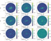 |
Fig. 3 Moment-0 maps of all the transitions for the source AG024.4614+0.1981. The color scales are in units Jy beam−1 km s−1. In the upper left panel, we show the continuum emission masks for reference. The red contour shows the mask of all the compact sources inside the source. The white contour shows the mask of the continuum emission with an S/N higher than 3. |
4.4 Details of the application of astroHOG
In this paper, we investigate how the emission of different species is correlated with the dust continuum emission. Moreover, it is interesting to explore if and how this correlation changes at different spatial scales. In particular, we want to investigate the level of correlation in the clump medium, which is traced by the extended diffuse continuum emission, and in the denser fragments which are traced by the compact dust emission. For this reason, we run astroHOG both on the mask of the extended emission (all pixels with the emission of continuum above 3 S/N, maskext.) and on the mask of all the compact structures that we identified with the CuTEx algorithm (maskcom.) for each target. More details on the creation of these masks are given in Appendix A. The continuum emission, with the masks defined, are shown in Fig. 4 for six sources as examples of the variety of emission morphologies in the sample. In some cases, especially for fainter sources, part of the extended emission might not be recovered due to the sensitivity limitation. The size of maskext. with respect to maskcom. varies from source to source, with six extreme cases in which ![Mathematical equation: $\[N_{\text {ext. }}^{\text {mask}}<2 ~N_{\text {com.}}^{\text {mask}}\]$](/articles/aa/full_html/2025/07/aa52700-24/aa52700-24-eq15.png) , where
, where ![Mathematical equation: $\[N_{\text {ext. }}^{\text {mask}}\]$](/articles/aa/full_html/2025/07/aa52700-24/aa52700-24-eq16.png) and
and ![Mathematical equation: $\[N_{\text {com.}}^{\text {mask}}\]$](/articles/aa/full_html/2025/07/aa52700-24/aa52700-24-eq17.png) are the number of pixels in the two masks (see bottom row of Fig. 4). For these six sources we considered only the maskcom. for the analysis.
are the number of pixels in the two masks (see bottom row of Fig. 4). For these six sources we considered only the maskcom. for the analysis.
To give some reference numbers, the median value of the area covered by maskcom. is of 0.004 pc2, while the median for maskext. is of 0.04 pc2. Both masks possibly include regions with outflows in the molecular emission. This is more relevant for maskext., but depending on the geometry of the outflows and how close from the compact source the shock is present, may also affect maskcom. A full disentanglement of the two masks from the regions with outflow emission (i.e., masks of extended/compact emission not co-spatial with outflows, and a mask only covering the outflow regions) would require a prior dedicated study on outflows to obtain the region covered by it, which is beyond the scope of this paper.
We expect that in some cases, the continuum emission of high-mass star forming regions at 1.38 mm is not only due to thermal dust emission, but may have a contribution from free-free emission. Therefore, we checked for available ALMAGAL counterparts in the CORNISH survey at 5 GHz (Purcell et al. 2008; Hoare et al. 2012). We identified 112 matched clumps, mostly evolved clumps (i.e., L/M > 10 L⊙/M⊙), compatible with the potential presence of HII regions. We do not exclude those clumps from the main analysis presented in the paper, since we do expect that the free-free emission will affect the emission of a small region inside each clump. However, we present in Appendix E the same results from the HOG analysis excluding the sources associated with a CORNISH counterparts, to show that the main conclusions of this work are not affected. We show in the same appendix that the inclusion of the 97 sources with moment-0 maps created over the fixed ±5 km/s range (which do not include the totality of the emission of the transition for the pixel of the line-rich cores and in the pixels with high-velocity wings) do not affect the results either.
We also expect that in some clumps the line emission in a portion of the map could be optically thick. However, this still provides information about how well the line is tracing the continuum, therefore we do not exclude sources due to optical depth consideration.
To compare the morphological emission of the line tracers considered in this work with the continuum emission, we derive the VN parameters from astroHOG and the Spearman correlation coefficient, ρs. The latter is a statistical correlation coefficient that determines if two sets of data, xi and yi, are well correlated from their intensity values.
We compute the correlations of the moment-0 maps and the continuum maps only on the intersection mask between the moment-0 emission masks defined in Sect. 4.2 and the continuum emission masks defined here and Appendix A, for both the HOG method and the Spearman coefficient correlation. This choice was made considering that in determining VN, the area where only one of the two maps shows emission, while the other is only noise, should contribute with a value close to 0. Thus, the VN value would be lowered by the percentage of the area of the map where only one of the tracers is detected.
To have robust and reliable results, for the intersection with maskcom. we took all the compact sources that have at least 60% of their area covered also by line emission, and checked that the pixels in the masks cover at least three times the area of the beam; for maskext. we performed the analysis only if the intersection with the mask of moment-0 covers at least five times the area of the beam and if the number of pixels of the intersection is at least two times the number of pixels of the mask derived from the intersection of maskcom. Lastly, to obtain an error estimate on VN, we used the MC method calculating 100 times VN to derive its error (see Section 4.3). The noise maps considered in the MC method are not correlated below the beam size, unlike the noise of interferometric maps. However, the value of correlation of the real noise in our dataset is below 3% (see Appendix B), and the correlation in the noise is not relevant in the regions with S/N>3 considered inside our masks.
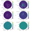 |
Fig. 4 Examples of continuum emission for six sources in the ALMAGAL sample. Upper row: continuum maps of two example sources with large diffuse emission outside the cores. Middle row: continuum maps of two example sources for which the diffuse emission is present but more restricted in area. Lower row: continuum maps of two example sources in which the continuum emission is well described by the mask of all compact sources only (the maskext, is plotted in dashed white for reference). Red contour: maskcomp., white contour: maskext. (see Section 4.4). The continuum image color scales are in Jy/beam. |
5 Results
5.1 Statistics of the detections in moment-0 maps
In this section, we analyze the statistics of the detection of the different molecular transitions, starting from the emission of the moment-0 maps. The number of clumps where a specific tracer is detected is given in Table 2 together with the corresponding percentage of the total sample, which is also shown in Fig. 5. Moreover, Table 2 and Fig. 5 show the percentage of detections when dividing the sample into five ranges of luminosity-to-mass ratio (L/M), a distance independent evolutionary indicator (Molinari et al. 2008, 2016, 2019; Giannetti et al. 2017; Elia et al. 2017, 2021; König et al. 2017). Sources with L/M < 1 L⊙/M⊙ are considered starless candidates. Considering the large number of sources in the ALMAGAL sample, we divided them into five ranges, to explore also very young sources (L/M < 0.1 L⊙/M⊙) and the most evolved (L/M > 100 L⊙/M⊙) ones.
Part of the differences in the detection statistics, and of the increase of the detection rate with L/M, originates from the chemical pathways that lead to the formation of these molecular species, which we reviewed in Section 2.2.
Together with the chemistry taking place, to interpret the difference in the detection rate for different molecular transitions, we have to consider that the critical density, ncrit, and upper state energy, EU/κB (where κB it the Boltzmann’s constant), of the selected transitions play a role in their detectability. These two parameters are listed in Table 1, except for the critical density of CH3OCHO since there are no collisional cross sections available for the E-conformer. The molecule with the highest detection rate clearly is H2CO with 76% in the H2CO 30,3−20,2 transition and 56% in the 32,1−22,0, which is the molecular species that form both in gas-phase and on grains and that can be released from the grains at the lowest temperature, and also in shock regions thanks to sputtering of the grains. The highest detected transition has the lowest upper energy of all the transitions analyzed in the sample (20 K), while H2CO 32,1−22,0 has an upper energy of 68 K. After H2CO, the most detected transitions are those of SO, CH3OH, and SiO with a detection rate of ~60%. The formation of those molecular species happens on grains, or through rapid gas-phase reactions after the release of some precursor atoms/species, and are then released thanks to sputtering or thermal desorption. The specific transitions analyzed in this paper, also have similar upper energy transitions between 30 K and 45 K. DCN 3–2 has a detection rate of 42% over the entire sample, despite having one of the lowest EU/κB. However, the abundance of this molecular specie is enhanced in warm/hot gas through gas-phase reactions, it is a deuterated species, and the specific transition has the highest critical density among the transitions analyzed. The three least detected molecular transitions are those of HCCCN, CH3CN, and CH3OCHO, respectively. The abundances of these molecular species are mainly enhanced in hot gas thanks to their release from grains at temperature above 90 K, therefore they are mostly detected only on the more evolved sources in the sample. CH3OCHO is the most complex molecular species in the sample, which is also the least detected. The detection rates of the different transitions as a function of EU/κB and ncrit, calculated for a gas temperature of 20 K, are given in Fig. 6. From the image, the percentages of detection within the total sample show a clear decreasing trend with EU/κB for values up to 70 K, together with a decreasing trend with ncrit, as highlighted by DCN 3–2.
The percentage of detections as a function of L/M varies noticeably for each molecular species. The detection rate increases for all species from the lower value of L/M to the highest ones, where all of the molecular transitions except of CH3OCHO show at least a detection rate of ~87%.
From the lower panel of Fig. 7, we note that H2CO (both transitions), CH3OH, SiO, and SO have already detection rates above ~25% in the less evolved sources (L/M < 0.1 L⊙/M⊙), with H2CO 30,3−20,2 reaching already more than 50%. This high detection is expected for H2CO that can desorb at ~40 K from grains and have gas-phase creation pathways, and CH3OH which has already been found in cold environment, despite a high desorption temperature. The 24% and 34% detection rate of SO and SiO can could be related to the higher efficiency of outflow observations to reveal the star-formation process from its very beginning compared to the infrared emission (e.g., Motte et al. 2007; Li et al. 2020; Towner et al. 2024) or to the presence of a narrow Gaussian component of SiO and SO in star-forming regions (e.g., Motte et al. 2007; Sanhueza et al. 2013; Duarte-Cabral et al. 2014; Csengeri et al. 2016), whose origin is caused by low-velocity shocks from cloud-cloud collisions, but not fully understood yet. The presence of outflow in very early stages could have also contributed to part of the high detection rate detected in H2CO and CH3OH. However, disentangling the two components as well as the identification of outflows is beyond the scope of this paper and will be explored in forthcoming papers of the ALMAGAL collaboration.
On the other hand DCN, HCCCN, CH3CN, and CH3OCHO have a statistics of detection lower than 8% for L/M below 0.1 L⊙/M⊙, since their chemical pathways require high temperature for their formation/release in gas-phase. The increase of the detection rate of these molecular species is thus more sensible (the trend is steeper) to the evolutionary stage and also the mean temperature of the clump (see upper panel of Fig. 7), as derived by Elia et al. (2017, 2021) from the SED fitting of the 160–850 μm continuum emission.
Number of clumps with a detection from the moment-0 maps.
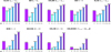 |
Fig. 5 Percentage of detection per clump of the molecular transitions for the whole sample and divided in ranges of L/M. The molecular transitions are sorted by the detection rate over the whole sample. |
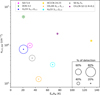 |
Fig. 6 Percentage of detection on the whole sample of the molecular transitions, shown as the diameter of the circles, in a scatter plot of the upper state energy transition and of the critical density at 20 K of the transition. |
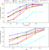 |
Fig. 7 Increase in the detection statistic of the molecular transitions, divided into bins of temperature of the clump (upper panel) and evolutionary stage of the clump L/M (lower panel). |
5.2 Area of the line emission versus the area of the continuum emission
In this section, we discuss the area of emission of the selected molecular lines with respect to the area of the emission of the continuum at the two levels (extended continuum and emission of the compact sources) defined by the mask presented in Sect. 4.4. In Fig. 8, we display for each molecular transition the histogram of the percentage of the area of maskext. covered also by the emission in the moment-0 map (in blue), the percentage of the mask of the emission of the moment-0 map covered by the maskext, and the percentage of dense cores detected in the molecular line (i.e., cores with at least 60% of the area covered by the moment-0 mask of the selected transition, in yellow). Only H2CO, CH3OH, and SO, already all known to be tracing also outflows, have at least 25% of sources with detection for which the molecular line emission covers more than 25% of the extended continuum mask. In particular the percentage is of 66%, 40%, 38%, and 27% for H2CO 30,3−20,2, SO, CH3OH, and H2CO 32,1−22,0, respectively. On the other hand, HCCCN, CH3CN, and CH3OCHO only have 11%, 7%, and 1% respectively of sources that cover more than 25% of the extended continuum mask. DCN and SiO have an intermediate number of sources around ~20% for which their emission cover at least 25% of the extended continuum mask. The fact that DCN can, in some sources, trace not only the dense emission, but also be present in diffuse gas, and also be easily detected at an advanced stage of the star-formation process and trace outflows has also been shown by Sakai et al. (2022), Cunningham et al. (2023), and Gieser et al. (2021), likely due to warm gas phase reactions occurring (Roueff et al. 2007).
Also, in the case of SiO emission, only 20% of the sources cover more than 25% of the area of maskext.. Thus, SiO shows a different overall emitting region than SO, even though both are outflow tracers. The reasons for the low percentage of SiO coverage of the extended continuum emission mask do not imply that SiO does not have extended emission, but that in most cases, this is mainly not in the region that overlaps the continuum emission. The purple histogram of SiO shows the largest percentage of sources for which less than 50% of the moment-0 map is covered by the mask of the extended continuum emission compared to all the other molecular species, including the other outflow tracers SO, H2CO, and CH3OH.
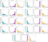 |
Fig. 8 For each molecular transition, three histograms are presented. The blue histogram shows the percentage of maskext. covered by the moment-0 mask of the selected transition. The purple histogram shows the percentage of the moment-0 mask of the selected transition covered by the maskext.. The yellow histogram shows the percentage of compact sources in which the transition is detected, that is compact sources with at least 60% of the area covered by the moment-0 mask of the selected transition. |
5.3 AstroHOG results
The results of the morphological comparison between the continuum emission and the emission of the molecular lines selected in this paper with astroHOG are shown in Fig. 9 and are tabulated in Tables D.1 and D.2, for the first 40 sources for the lines of H2CO on the maskext. and maskcom., respectively. The full versions of Tables D.1 and D.2 and the analogous Tables for all the other molecular lines are available through Zenodo. The top row of Fig. 9 shows the results from the comparison with the diffuse emission (maskext.), while the bottom row shows the same results with the dense emission (maskcom.). Moreover, in Fig. 10 we plot only the median values of the histograms presented in Fig. 9. Values of VN above 0.02 deviate from the statistical correlation that can be found running astroHOG on noise maps (see Appendix C), and are considered significant. The same plot excluding sources with CORNISH counterparts, that is, excluding possible free-free contamination in the continuum emission, or with only the sources for which moment-0 maps have been created selecting a fixed range of +/−5km/s range are presented in Fig. E.1, and shows no significant variation from the main results of Fig. 10.
As shown in the previous section, only H2CO (both transitions), CH3OH, and SO cover in more than the 25% of the sources at least 25% of the area of maskext.. The two transitions of H2CO and CH3OH have similar median values, 0.27–0.29 (27–29%), while the median morphological correlation of SO with the continuum at the diffuse scale is 0.24 (24%). These percentages highlight that on average these transitions do not trace well the continuum emission arising from the diffuse thermal dust emission. In fact, these numbers can be interpreted as saying that only 24 to 29% of the area compared is morphologically well correlated on average. We report the results also for the rest of the molecular transitions, but the results of the previous section should be kept in mind, that is, that SiO and DCN have only 20% of the sources covering more than 25% of the area of maskext., while for the rest of the molecular species the percentage is below 10%. Therefore the results of the astroHOG on maskext. are in general for this transitions limited to a smaller area. SiO shows the lowest value of correlation, with a median value of 0.15 (15%). This value is the lowest in the entire sample of transitions analyzed. On the other hand, the results for HCCCN, DCN, and CH3CN are ~0.5 (50%), while for CH3OCHO (for which we have only 17 sources, while in the other case we always have more than ~150 following the selection criteria on the masks detailed in Section 4.4) we found a value of 0.84 (84%). These considerations should be taken statistically over the source sample, since for all species we find some specific sources in which VN is very close either to 0 or to 1 (100%).
For the comparison on compact continuum emission, the molecular transition with the lowest value of morphological correlation is again SiO, with a median correlation of 0.35 (35%). The other molecular species can be divided in two groups. The first group consists of H2CO (both transitions), CH3OH, and SO. For this group, we found mediancorrelation values of around 40%, with an increase between the values found for the same molecular transitions at the diffuse scale. However, these molecules, even at the scales and densities of the cores, do not present the same morphology of the continuum emission.
The second group of molecules, which includes HCCCN, CH3CN, DCN, and CH3OCHO, show a very high correlation with the morphology of the continuum at the dense cores scales. For these molecules, the value of the normalized projected Rayleigh statistic is in the range 62–65%, with the exception of CH3OCHO, which has a median value of 87%. CH3OCHO and CH3CN (respectively an O-bearing and an N-bearing molecule) are the two tracers with the best agreement in morphology with the compact continuum. Most of the transitions considered for these molecules have values of EU/κB at the higher end of the range covered by all the transitions analyzed in this paper, with the exception of the transition of DCN (from Table 1 the DCN 3–2 line has EU/κB ~ 21 K), which still shows a high degree of morphological correlation. Moreover, in the first group of molecules we also find the transition of H2CO 32,1−22,0 which has a value of EU/κB similar to those of CH3CN, but still has a low correlation with the continuum morphology (below 50%). We therefore conclude that the difference between the two groups of molecular transitions is related to the molecular species. However, some bias due to the selected transition is present especially on the compact mask.
We analyzed two lines of H2CO with two different EU/κB (21 K and 68 K, respectively). The results show a mild improvement in the morphological correlation with the continuum using the transition with higher EU/κB at the extended scale, but at this scale it is quite consistent with the other transition, while a larger increase (from 31% to 45%) is seen at the scale of the compact sources. A dependence on the selected transition is present. Therefore, the results of this paper can be considered valid also for other transitions of the same molecular specie, in a reasonable range of EU/κB around the transitions presented here.
The difference between the two groups of molecules can be traced back to their mechanism of formation (see Section 5.1), together with the conditions of excitation of the selected transition. SiO, whose formation pathway is strictly linked to sputtering of dust grains in shock/outflows regions, register the lowest morphological correlation with the continuum emission. All the other three molecular species that show a low level of morphological correlation are species that have been shown to be associated to shocks. At the scale of compact emission these molecular species have a higher degree of correlation, but still below 50%. In this case, the main emission could likely come not only from the cores but also from an outer envelope surrounding them, since the conditions of the release of these molecular species and/or the low/intermediate excitation temperature allow their emission. Still, a contribution to outflows close to protostellar objects can be present also at core scales. The comparison of SO and SiO on both masks shows a difference between the two molecules, as already highlighted by the results of Section 5.2. In fact, SO has in general values closer to those of H2CO and CH3OH. This is likely due to the importance of the formation route of SO after the thermal desorption of H2S from dust grains due to thermal desorption. On the other hand, DCN, HCCCN, CH3CN and CH3OCHO have pathways of formation that require high temperature for their formation/release in gas phase. The higher values of the upper energy of the transitions (with the exception of DCN) also contribute to the fact that they probe the warm/hot gas linked to the evolved cores, without contribution from their colder outer envelope, thus showing a good morphological correlation with the continuum over the maskcom.. These molecular species shows less extended emission, as seen in Sect. 5.2, but the area of extended continuum emission, which in some cases is covered by their emission, show an intermediate level of correlation ~50%.
We also explored the possible dependence of the results of the morphological correlation of the selected transitions with the dust continuum emission with the evolutionary stage of the clumps, dividing the sample in three range of L/M: L/M < 1 L⊙/M⊙, 1 L⊙/M⊙ < L/M < 10 L⊙/M⊙, and L/M > 10 L⊙/M⊙. The results are shown in Fig. 11. In general, the distributions of the morphological correlation of almost all the molecular lines with the continuum for the three evolutionary stages, are consistent within the errors. The only clear differences are for HCCCN and CH3CN for L/M<1 in the maskext.. However, the statistics for these two points are based on ten or less sources. The fact that we found no correlation with the evolutionary stage of the clump, indicated by the L/M value, could not exclude a possible dependence with the evolutionary stage of the single fragments forming inside the clump itself. In fact, a clump can contain fragments in different evolutionary stages (especially for sources with high values of L/M). No in-depth analysis of the evolutionary stages of the cores, that considers the temperature of the cores or the outflows originating from them is available so far. Therefore, the mask comp that include all the cores, can mix together cores in different evolutionary stages, including both starless and protostellar cores. This is true also for maskext, which can contain emission from the starless cores and their surroundings together with the emission from more evolved and dynamical regions. For this reasons, a possible dependence with the evolutionary stage of the individual cores might be undetectable, due to mixing of the two in the same masks. For some of the molecular species, such as CH3CN and CH3OCHO there could also be no difference due to a selection effect, that is, the cores with emission of these molecular species in all the range of L/M are in the same phase, i.e. already protostellar objects with high temperature at their center, therefore the different L/M bins, which probe different evolutionary stages at clump level, in these cases might still be probing cores at the same stage of evolution.
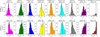 |
Fig. 9 Morphological correlation between the continuum emission and the line emission (moment-0) for the indicated transition, as quantified by VN parameter from the astroHOG method. Values of VN ≈ 0 and VN ≈ 1 correspond to no correlation and perfect correlation in the distribution of the two emissions, respectively. The upper panels correspond to the correlation on the intersection of the moment-0 line emission mask and the maskext.. The lower panels correspond to a mask selecting only the compact sources where the line is detected, starting from maskcom.. The dotted and dashed histograms represent how the distribution would change if all the values were replaced by VN − error (the error on the value of VN is derived using an MC method, see Sect. 4.3) and VN+ error, respectively. |
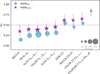 |
Fig. 10 Median value of VN histograms for the maskext. (light blue points) and for the maskcom. (purple stars) for the different molecular transitions. The horizontal dashed line represent the values of VN for which ~50% of the area has a good agreement in the two maps (continuum and moment-0). |
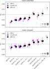 |
Fig. 11 Upper panel: median value of VN histograms for the maskext. dividing the sample into three evolutionary stages; lower panel: median value of VN histograms for the maskcom. dividing the sample into three evolutionary stages. The horizontal dashed line represent the values of VN for which ~50% of the area has a good agreement in the two maps (continuum and moment-0). |
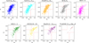 |
Fig. 12 Comparison between the Spearman correlation coefficient and the VN parameter from the HOG method in the comparison between the continuum and the indicated species using maskext.. The two boxes delimited by red dotted-dashed lines are the regions in the plot where the two estimators give the more contrasting results. |
5.4 Comparison with the Spearman correlation coefficient
In this section we compare the results obtained with the HOG method with one of the most widely used tool in the literature for computing the correlation between two tracers: the Spearman correlation coefficient, ρs. The definition of this coefficient starts from those of the Pearson correlation coefficient, ρp, which determines whether two data sets, xi and yi, are well correlated through a linear relation. The parameter ρp is defined as
![Mathematical equation: $\[\rho_{\mathrm{p}}=\frac{\sum_i\left(x_i-\hat{x}\right)\left(y_i-\hat{y}\right)}{\sqrt{\sum_i\left(x_i-\hat{x}\right)^2} \sqrt{\sum_i\left(y_i-\hat{y}\right)^2}},\]$](/articles/aa/full_html/2025/07/aa52700-24/aa52700-24-eq18.png) (6)
(6)
where in our case, datasets xi and yi are the pixel-to-pixel intensities of the selected moment-0 map and of the continuum map of the source, and ![Mathematical equation: $\[\hat{x}\]$](/articles/aa/full_html/2025/07/aa52700-24/aa52700-24-eq19.png) and
and ![Mathematical equation: $\[\hat{y}\]$](/articles/aa/full_html/2025/07/aa52700-24/aa52700-24-eq20.png) are their mean values. Therefore, this statistical correlation coefficient is intensity based, unlike the HOG method, which is gradient based, and imply an underlying linear correlation between the two datasets.
are their mean values. Therefore, this statistical correlation coefficient is intensity based, unlike the HOG method, which is gradient based, and imply an underlying linear correlation between the two datasets.
In the case of the Spearman coefficient, no underlying linear relation is assumed, and it is defined as the Pearson correlation coefficient between the rank variables, that is, the variables that report the rank in order or brightness for each pixel of the two maps.
We present here the Spearman coefficient results only, which is the most suitable to use, but we tested also the Pearson correlation coefficient, and the values are given in Tables D.1 and D.2 and on Zenodo2. In general, the Pearson correlation coefficient gives fairly similar results to those of the Spearman correlation coefficient in comparison with astroHOG.
We compute ρs using the same masks used for the HOG method, and Figure 12 shows the comparison of the results of this method with the HOG method on the maskext. for all the species and in Figure 13 for all the species on the maskcom.. The results of the statistical correlation coefficient do not differ much from the results of the HOG method, and in general, there is an underlying positive correlation among the results of them with the HOG method, but a high degree of scatter is found. For high values of ρs ~ 0.7, there is a large spread in VN with some values below 0.5. For some points the two methods even give clearly contrasting results (see the two areas in the upper-left and lower-right corner of each plot in Figs. 12 and 13: VN > 0.5 and ρs < 0.3 and VN < 0.2 and ρs > 0.6). The majority of the sources with highly contrasting results between the two methods fall in the upper-left corner of the plots, that is, in the region where from the Spearman correlation coefficient there is a moderate/high correlation, but a very low correlation based on the HOG results, which means that even if there is a good level of correlation in the intensity of the continuum and the molecular species, the two emissions do not have a similar morphology. An example is given in Fig. 14, where we show both the continuum map and the moment-0 map of H2CO 30,3−20,2 for AG019.8843-0.5337 with the direction of the gradients, together with the scatter plot of the intensity from which the Spearman correlation coefficient is calculated. The gradients do not in general match well as indicated by the value of VN, and also the majority of the points in the scatter plot do not show a linear trend. The trend that results in ρs ~ 0.67 is driven by a small number of points that correspond to the brightest source in the continuum, which is also the brightest in the moment-0 map. The ρs is therefore mostly biased by a small number of good matching points due to the dynamic range of the values of intensity. This effect is relevant also for the Pearson correlation coefficient, having a value of 0.69 in this case.
Figure 15 shows an example of one of the clearest opposite (less common) cases, where VN has high values, while ρs is very low. In clump AG332.7016-0.5870, the morphology of H2CO 32,1−22,0 and the continuum on the cores for which H2CO 32,1−22,0 is detected match well (in the gradients, VN = 0.64), but the brightest source in the continuum does not correspond to the brightest source in H2CO 32,1−22,0 emission. Therefore, the value of the intensity-based correlator ρs is ~0.07 in this case. This example shows that the two types of statistical correlators give different results, and are suited to answer different questions. If the main goal is to compare the morphology of two tracers, the HOG method is to be preferred to intensity-based correlator. On the other hand, if the goal of a study is to determine if two tracers peak at the same positions the latter is the most suitable. Moreover, the values of intensity-based correlator should be carefully checked in case of maps with large dynamical range.
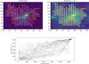 |
Fig. 14 Example of a source for which the HOG method indicates a low morphological correlation and the Spearman correlation indicates a high correlation. The source is AG019.8843-0.5337 and in the comparison of the continuum and of the moment-0 of H2CO 30,3−20,2 in the maskext. VN=0.20, while ρs = 0.67. The two panels in the upper row show the continuum and the moment-0 map of H2CO 30,3−20,2 with superimposed the directions of the gradients in the two maps (red: moment-0, white: continuum, respectively). The panel in the lower row shows the scatter plot of the pixel-to-pixel rank variables in the two maps inside the same mask (in black in the images of the two maps) where both the Spearman correlation and the Projected Rayleigh Statistic, VN, have been computed. |
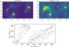 |
Fig. 15 Example of a source for which the HOG method indicates a high morphological correlation and the Spearman correlation coefficient indicates a low correlation. The source is AG332.7016-0.5870 and in the comparison of the continuum and of the moment-0 of H2CO 32,1−22,0 in the maskcom. VN=0.64, while ρs=0.07. The two panels in the upper row show the continuum and the moment-0 map of H2CO 32,1−22,0 with superimposed the directions of the gradients in the two maps (red: moment-0, white: continuum, respectively). The panel in the lower row shows the scatter plot of the pixel-to-pixel rank variables in the two maps inside the same mask (in black in the images of the two maps) where both the Spearman correlation and the Projected Rayleigh Statistic, VN, have been computed. |
6 Conclusions
We analyzed the integrated emission of lines from eight of the most commonly detected molecular species (i.e., H2CO, CH3OH, DCN, HCCCN, CH3CN, CH3OCHO, SO, and SiO) in the largest survey of high-mass star-forming clumps ever observed at high angular resolution, the ALMAGAL survey. To evaluate how well these species trace the cold dust, we used an innovative method, the histogram of oriented gradients (HOG, with the package astroHOG), which quantifies the level of similarity in the morphology of two images. The method only uses the angle between the gradients in the two images to derive the level of correlation, and it is completely independent of the intensity values of the two images as well as the intensity of the gradients. We compared the morphology of the moment-0 maps of these tracers with the dust continuum emission at 1.38 mm using the HOG method on two spatial scales of the extended emission and of the compact sources alone. We also compared the results of this method with those obtained using the Spearman correlation coefficient, which is an intensity-based correlator. We summarize the main results below:
The detection rate of all the molecular species increases with the L/M ratio of the sources to reach a detection percentage close to or above 87% for sources with L/M > 100 L⊙/M⊙. The exception is CH3OCHO, which is only detected toward 110 sources in our entire sample;
Only the emission of H2CO, CH3OH, and SO covers the extended continuum (maskext.) in a large fraction of sources. The smallest fraction is observed for SiO, where the extended emission, if present, is mostly not cospatial with the continuum emission. This is expected since SiO is mainly emitted in the outflow lobes, where continuum from cold dust is not observable. This highlights a difference between SO and SiO, based on which the former is to be considered not only as a shock tracer. Moreover, in some sources (the exact number might be limited by the sensitivity of the data), DCN is not only detected toward the compact cores, but also shows extended emission;
Even though H2CO, CH3OH, and SO cover the extended continuum emission, the morphological comparison using the HOG method (astroHOG) showed a low level of correlation. Only 24–29% of the area in which both emissions are detected agree well morphologically.
The analysis on the compact fragments shows that DCN, HCCCN, CH3CN, and CH3OCHO are strongly correlated morphologically with the compact continuum emission. The values exceed 60%. On the other hand, SiO has the lowest correlation with the compact continuum emission, followed by H2CO, CH3OH, and SO, which still has low to intermediate values of correlation (below 45%);
The results of astroHOG divided into three bins of the evolutionary indicator L/M show no clear differences in the morphological correlation with the evolution of the clump. This result might be biased because inside each clump, cores in prestellar and protostellar phase might be mixed together. This effect is not observed for some of the molecular species, whose emission only arise from more evolved cores/regions inside the clump, that is, for HCCCN, CH3CN, and CH3OCHO. The similarity of the HOG results in all the evolutionary stages of the clump in these three species might be due to a selection effect that includes only the more evolved cores inside the analysis in all the bins of L/M;
The trend between the HOG result (VN) that correlates the general emission morphology and the Spearman coefficients (ρs) that only measure the correlation of the intensity is positive. The scatter is large, however, and for some sources the results of the two methods clearly differ. Due to their intrinsic nature, the two types of methods are best suited to answer different questions, with the HOG method better performing in comparison of morphologies.
Based on these results, we roughly divided the molecular transition into two classes. The first class is composed of H2CO, CH3OH, SO, and SiO transitions. They do not trace the same morphology as the continuum both on the extended and compact emission scales. Moreover, the SiO emission differs from that of the other outflow tracers. This was confirmed by the percentage of the overlap of SiO emission and continuum emission, compared with the same values for the other tracers, and by the results of astroHOG. We will present a direct comparison using astroHOG of the moment-0 maps of different molecular species, to investigate this aspect as well in a forthcoming paper.
The second group of molecular transitions contains lines of DCN, HCCCN, CH3CN, and CH3OCHO, which do not trace the most diffuse part of the continuum emission in most sources, but are morphologically well correlated with the compact dust continuum emission. The exception in the latter category is DCN, whose emission traces part of the diffuse emission toward ~20% of the sources compared to less than 10% in the other molecular lines in this group.
These results are to be considered valid in a reasonable range of EU/κB values around those of the transitions presented here, since we have seen a dependence with the excitation temperature of the transitions for the two lines of H2CO, especially in compact sources.
The total detected emission that is cospatial with the densest fragments for the species with a low level of correlation in the fragment mask indicated that these molecular transitions strobgly contribute emission from the intraclump medium or from outer layers around the fragments (in some cases, this might also be due to optical depth effects). In contrast, the total emission toward the densest fragments of species with strong morphological correlation is dominated by the emission from the fragments themselves.
Data availability
The Tables of results are available for the entire sample on Zenodo: https://doi.org/10.5281/zenodo.15236491
Acknowledgements
C.M. and the INAF-IAPS team acknowledge funding from the European Research Council (ERC) under the European Union’s Horizon 2020 program through the ECOGAL Synergy grant (ID 855130). R.K. acknowledges financial support via the Heisenberg Research Grant funded by the Deutsche Forschungsgemeinschaft (DFG, German Research Foundation) under grant no. KU 2849/9, project no. 445783058. P.S. was partially supported by a Grant-in-Aid for Scientific Research (KAKENHI Number JP22H01271 and JP23H01221) of JSPS. P.S. was supported by Yoshinori Ohsumi Fund (Yoshinori Ohsumi Award for Fundamental Research). C.B. gratefully acknowledges funding from National Science Foundation under Award Nos. 2108938, 2206510, and CAREER 2145689, as well as from the National Aeronautics and Space Administration through the Astrophysics Data Analysis Program under Award “3-D MC: Mapping Circumnuclear Molecular Clouds from X-ray to Radio,” Grant No. 80NSSC22K1125. A.S. M. acknowledges support from the RyC2021-032892-I grant funded by MCIN/AEI/10.13039/501100011033 and by the European Union ‘Next GenerationEU’/PRTR, as well as the program Unidad de Excelencia María de Maeztu CEX2020-001058-M, and support from the PID2023-146675NB-I00 (MCI-AEI-FEDER, UE). RSK acknowledges financial support from the ERC via Synergy Grant ECOGAL (project ID 855130), from the German Excellence Strategy via the Heidelberg Cluster “STRUCTURES” (EXC 2181 – 390900948), and from the German Ministry for Economic Affairs and Climate Action in project “MAINN” (funding ID 50OO2206). RSK also thanks the 2024/25 Class of Radcliffe Fellows for highly interesting and stimulating discussions. Part of this research from D.C.L. was carried out at the Jet Propulsion Laboratory, California Institute of Technology, under a contract with the National Aeronautics and Space Administration (80NM0018D0004). LB gratefully acknowledges support by the ANID BASAL project FB210003. This paper makes use of the following ALMA data: project code 2019.1.00195. L. ALMA is a partnership of ESO (representing its member states), NSF (USA) and NINS (Japan), together with NRC (Canada), MOST and ASIAA (Taiwan), and KASI (Republic of Korea), in cooperation with the Republic of Chile. The Joint ALMA Observatory is operated by ESO, AUI/NRAO and NAOJ.
Appendix A Masks creation
A.1 Continuum masks
In this paper, we created two different masks on the continuum maps.
The first mask we defined contains all the compact sources detected in the field of view by CuTEx, and we call it maskcomp.. CuTEx (Molinari et al. 2011) individuates compact sources inside continuum maps building a curvature image by double-differentiation of the initial map in four different directions. This method allows an easier identification (by applying a threshold on the curvatures maps) of compact sources, which stand out in the curvature images, while diffuse and background emission is strongly dampened. Identified peaks in curvature maps are then fitted (on the original map) with 2D elliptical Gaussians plus a background that can be a constant background (zero order) or an inclined plane (first order) background3, in order to obtain the position and dimensions of the sources (major axis σA, minor axis σB, and position angle) and the integrated flux background subtracted. As last step, we required that the background-subtracted peak flux from photometry is higher than five times the map rms to confirm the compact source. CuTEx has been run on the continuum 7M+TM2 maps using the same method as Coletta et al. (2025) for the 7M+TM2+TM1 maps (the catalog for 7M+TM2 will be presented in Coletta et al. in prep.). For the maskcom. we create ellipses for each core that took as semi-axis 2σA and 2σB from the 2D Gaussian fits, to recover the 86% of the integral of the source4. An example of maskcom. for the source AG024.4616+0.1981 is visible in red in the upper row of Fig. A.1
The second mask, which includes the most diffuse and extended continuum emission, is defined as the continuum emission with a S/N higher than 3, (maskext.). In the ALMA continuum map, the noise level is not uniform but increases from the center of the map toward the edge, following the shape of the primary beam. Therefore, we build a map of noise by estimating the noise level of the continuum image not corrected for the primary beam, where the noise is uniform all over the map, with a sigma clipping method and then we divided for the map of the primary beam. In the first step of the mask creation we select all of the pixels above an S/N of 3. In these first step a lot of noise peaks just above an S/N 3 are included in the mask. Therefore, as second step we excluded from the first raw mask all the isolated regions with a number of pixels < 0.8 × Nbeam, where Nbeam is the number of pixels inside the area of a beam. As third step we dilated the mask by one beam (Dame 2011), to encompass possible emission just below the 3 S/N threshold, and as final step we include all of the pixel of maskcom. in maskext., if case not all of them where already selected. The steps for the creation of maskext. are illustrated in orange in the second row of image A.1 for source AG024.4616+0.1981. The last step for this source is not needed, since all of the pixel of maskcom.. were already in maskext. at step 3.
A.2 Moment-O masks
For the moment-0 maps we derived a maps of the noise, using the same method as described above for the continuum maskext.. In the first step of the mask creation we select all of the pixels above an S/N of 3. Therefore, in the second and final step we excluded the regions that do not have any pixel with an S/N above 5 or that have a to- tal number of pixels < 0.8×Nbeam. The first requirement is connected to the fact that integrated line intensity below a 5 S/N would result in spectral lines not identified above a 3 S/N in the spectrum, while the second is to avoid spurious noise fluctuation peaks in the mask. As the last step, we required that at least one of the regions remaining inside the mask has a number of pixels > Nbeam, since this would be the size of emission of a point-like source. If this last condition is met, we considered the transition as detected in the field. The two steps for the creation of the moment-0 mask for the transition of H2CO 30,3−20,2 for source AG024.4616+0.1981 are visible in the first two columns of the bottom row of Fig. A.1 in white.
A.3 Intersection masks
We calculated the astroHOG VN coefficient and the Spearman coefficient on the intersection between the moment-0 mask and maskext.. An example is visible in the third column of the bottom row of Figure A.1. For the compact emission, we run the analysis on the mask of the compact cores with detection of the selected transition, that we defined as the cores that are covered by more than 60% by the mask of the moment-0 of the selected transitions. An example is visible in the last column of the bottom row of Figure A.1. In this case all the cores defined in the continuum met our condition.
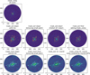 |
Fig. A.1 Figure illustrating the steps defining the masks used in this paper for source AG024.4616+0.1981 for the continuum and for the moment-0 of H2CO 30,3−20,2. Upper row: continuum maskcomp.; middle row: steps for the creation of continuum maskext.; bottom row first two panel from left: steps for the creation of the mask on moment-0; bottom row last two panel on the right: intersection masks used for the analysis. |
Appendix B Definition of the range of integration for moment-0 maps
In order to create the moment-0 maps for all the sources and all the selected transitions (1013 sources × 9 transitions), we created an automated routine that derives the best velocity range for integrating the cubes. The aim of the routine is to individuates the velocity range that encompass all the line (including high-velocity wings) in all the pixel of the source, to then integrate all the pixel over the same velocity range.
As first step, we resampled spatially the cube on the two positions axis by a factor 6, the average number of pixels in a beam size. For each source, we created an average spectrum from all the pixels with emission above 4σ (σ is the standard deviation of the cube along the frequency axis) in the resampled cube in an interval of 7 km/s around the systemic velocity of the clump, to avoid selecting a different line close in frequency, and we fit it with a Gaussian profile. We repeated the Gaussian fit for the spectrum of the pixel with the highest line intensity peak, since in some cases the line on the brightest pixel shows higher FWHM than the median spectrum defined before. We took the largest full width at half maximum (FWHMmax) of the two fits and the central velocity, vfit, of the first fit to define as integration limits vfit − 2FWHMmax, and vfit + 2FWHMmax. Moreover, considering the possible presence of non-Gaussian wings in strong lines, for pixels with emission above 5σ we calculated the initial and final endpoints of the wings (i.e., where the emission of the wings goes to zero) as the two values vi and vf where the signal-to-noise ratio (S/N), starting from the center of the line, goes below 0.5. This ensures that the full wing is included inside the integration, since in many cases wings are very noisy and the signal has channels below 1 S/N before the end of the wing. Finally, to compute the moment-0 maps, we adopt the starting point as the minimum value between vi and vfit − 2FWHMmax, and the endpoint as the maximum value between vf and vfit + 2FWHMmax. The CH3CN 120 − 110 and 121 − 111 lines are heavily blended in several sources. Therefore, for these two transitions, we created a single moment-0 map that includes the emission of both transitions, and then we fitted two Gaussian assuming they have the same FWHM.
In Figure B.1 we show the different spectra used for defining the extreme of integration for the line of H2CO 30,3−20,2 (upper row) and CH3CN 120,1−110,1 (bottom row) for source AG024.4616+0.1981. The first panel (from left) in the upper row shows the median spectrum of all the pixels above 4σ and its best fit. The value of the FWHM of this fit define the first guess for the extreme of integration (dashed vertical magenta line) shown in all the panels. The second panel shows the spectrum of the pixel with the highest peak intensity with its best fit. The value of the FWHM of this fit define the second guess for the extreme of integration (dashed vertical green line) shown in all the panels. The third panel show the spectrum of the pixel with more extended blue-shifted wings, with the blue vertical line indicating the channel where the emission of the blue-wing goes below 0.5 S/N. The last panel show the spectrum of the pixel with more extended red-shifted wings, with the blue vertical line indicating the channel where the emission of the red-wing goes below 0.5 S/N. As defined before, we then selected the largest extreme of integration to create the moment-0 maps, in this case the value defined by the blue and red solid vertical lines.
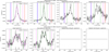 |
Fig. B.1 Steps of the determination of the range of integration for the moment-0 maps for the example source AG024.4616+0.1981 for H2CO 3(0,3)-2(0,2) (top row) and CH3CN 120,1 − 110,1 (bottom row). Top row from left: 1) mean spectrum over all the pixel with peak emission above 4 S/N, with its best fit and derived range of integration in magenta; 2) pixel with highest peak spectrum, with its best fit and derived range of integration in green; 3) spectrum of the pixel with the blue-wing terminating at the lowest velocity, marked by the blue vertical line; 4) spectrum of the pixel with the red-wing terminating at the highest velocity, marked by the red vertical line. Bottom row: same as top row, but for CH3CN 120,1 − 110,1 for which a 2-Gaussian fit is performed to include both K=0 and K=1 line. No spectra are shown in the last two panel since no pixel was found with wings above the integration range defined by the first two panels. |
The bottom row of Fig. B.1 shows the same spectra as the upper row, but for the case of CH3CN, where only one moment − 0 map have been created integrating together the transitions 120,1−110,1, since they are in most cases blended. For this reason the first two panels (from left) show a two-Gaussian fit, and the extreme of integration took into account the separation in veocity of the two peaks. For this source there are no pixels with blue-wing or red-wing above the range of integration already defined from the 2 two-Gaussian fit, so there is no spectra in the last two panels on the right. In this case the extreme of integration selected for the creation of the moment-0 map are those indicated by the vertical magenta dashed lines.
All the maps for each field and transition were then visually inspected to validate them. This was done by looking at the line observed in the spectra averaged on each continuum compact source detected by the source-extraction algorithm CUrvature Thresholding EXtractor (CuTEx; Molinari et al. 2011, 2016 see Sect. 4.4; following the same method as was used in Coletta et al. (2025) for 7M+TM2+TM1 data) in the clump, and checking that the velocity extremes used for the integration agree with the velocity ranges of the lines in these spectra, and no blending with other lines is present.
Appendix C Noise correlation in astroHOG
To estimate the significance of the projected Rayleigh statistics parameter VN, in output of astroHOG, we performed the morphological comparison on noise-only maps. We selected couples of moment-0 maps of the same sources of two non-detected lines, for a total of 50 couples of noise maps, and ran astroHOG on the total FOV of the maps. The list of moment-0 maps used and the results of astroHOG are given in Table C.1. The histogram of the values of VN from the correlation of noise-only maps is given in Fig. C.1, while in Fig. C.2 we plotted one couple of noise maps with over imposed the gradients directions in the two maps. The median absolute deviation of the correlation of noise-only maps is 0.6%, with all the values being below 3%.
Appendix D Tables of Results
In Tables D.1 and D.2 we give the results of astroHOG analysis, of the Pearson correlation coefficient, and the Spearman correlation coefficient, together with the number of pixels of the various masks adopted in the analysis for the first 37 sources for H2CO 30,3−20,2 for maskext. and maskcomp., respectively. The complete tables, as well as the tables for all of the other transitions are given in Zenodo5.
Results of astroHOG significance test on moment-0 maps with non-detection.
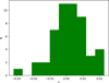 |
Fig. C.1 Distribution of the VN parameter, calculated by astroHOG on pairs of noise-only moment-0 maps. |
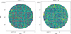 |
Fig. C.2 Gradients comparison on a pair of noise-only maps from Table C.1 for source AG023.0417+0.2925. The color scale units are Jy/beam km s−1 in both panels. The cyan lines indicate the direction of the gradients of the noise map in the left panel, while the red lines indicate the direction of the gradient of the noise map in the right panel. For this pair of noise maps VN is 0.013. |
Results of astroHOG, the Pearson correlation, and the Spearman correaltion for the maskext. for H2CO 30,3 − 20,2.
Results of astroHOG, the Pearson correlation, and the Spearman correlation for the maskcomp for H2CO 30,3 − 20,2.
Appendix E HOG results excluding failed automatic routine sources for moment maps and sources with CORNISH counterparts
In the main text we have presented the results of the analysis of the histogram of oriented gradients (HOG) in Fig. 9 on all the sources. However, for 97 sources we created the moment-0 maps using a fixed velocity range of +/ − 5km/s, since the automated routine failed due mostly to blendings in line-rich sources. The moment-maps of these sources therefore do not encompass the entire line in the pixels of the line-rich cores to avoid line blendings, and are not integrating possible high velocity wings also in less line-rich regions of the clump. In Figure E.1 we show that the inclusion of these sources, with moment-0 maps defined in a different way, do not alter the main result shown in the main text, since the differences between the results on all the sources (upper-left panel) and the results only on the 97 sources (upper-right panel) are negligible and well within the range of the distribution.
Moreover, for 112 sources we found a counterpart in emission from CORNISH. In these sources a part of the continuum emission could be affected by free-free emission. Since the importance of this contamination, both in the area of the maps affected, and in the relative importance in the flux measured, is not known, we show in the bottom row of Figure E.1 that removing these contaminated sources does not alter the main results shown in the text (and in the upper-left panel of Figure E.1).
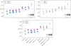 |
Fig. E.1 Top left panel: same of Fig. 9, that is, results of the astroHOG analysis on all the sample; top right panel: same plot only for the sources for which the automated routine for the creation of moment-0 maps failed; bottom panel: same plot excluding from all the sources those with a CORNISH counterpart. |
References
- Albertsson, T., Semenov, D. A., Vasyunin, A. I., Henning, T., & Herbst, E. 2013, ApJS, 207, 27 [CrossRef] [Google Scholar]
- Beltrán, M. T., Cesaroni, R., Rivilla, V. M., et al. 2018, A&A, 615, A141 [Google Scholar]
- Beuther, H., Zhang, Q., Sridharan, T. K., Lee, C. F., & Zapata, L. A. 2006, A&A, 454, 221 [NASA ADS] [CrossRef] [EDP Sciences] [Google Scholar]
- Bracco, A., Jelić, V., Marchal, A., et al. 2020, A&A, 644, L3 [EDP Sciences] [Google Scholar]
- Burke, D. J., Puletti, F., Brown, W. A., et al. 2015, MNRAS, 447, 1444 [CrossRef] [Google Scholar]
- Caselli, P., & Ceccarelli, C. 2012, A&A Rev., 20, 56 [NASA ADS] [CrossRef] [Google Scholar]
- Cesaroni, R., Pestalozzi, M., Beltrán, M. T., et al. 2015, A&A, 579, A71 [NASA ADS] [CrossRef] [EDP Sciences] [Google Scholar]
- Chacón-Tanarro, A., Caselli, P., Bizzocchi, L., et al. 2019, A&A, 622, A141 [Google Scholar]
- Charnley, S. B., Tielens, A. G. G. M., & Rodgers, S. D. 1997, ApJ, 482, L203 [NASA ADS] [CrossRef] [Google Scholar]
- Coletta, A., Molinari, S., Schisano, E., et al. 2025, A&A, 696, A151 [NASA ADS] [CrossRef] [EDP Sciences] [Google Scholar]
- Cosentino, G., Jiménez-Serra, I., Tan, J. C., et al. 2022, MNRAS, 511, 953 [NASA ADS] [CrossRef] [Google Scholar]
- Csengeri, T., Leurini, S., Wyrowski, F., et al. 2016, A&A, 586, A149 [NASA ADS] [CrossRef] [EDP Sciences] [Google Scholar]
- Cunningham, N., Ginsburg, A., Galván-Madrid, R., et al. 2023, A&A, 678, A194 [NASA ADS] [CrossRef] [EDP Sciences] [Google Scholar]
- Dame, T. M. 2011, arXiv e-prints [arXiv:1101.1499] [Google Scholar]
- Duarte-Cabral, A., Bontemps, S., Motte, F., et al. 2014, A&A, 570, A1 [NASA ADS] [CrossRef] [EDP Sciences] [Google Scholar]
- Durand, D., & Greenwood, J. A. 1958, J. Geol., 66, 229 [Google Scholar]
- Elia, D. 2020, Commun. Byurakan Astrophys. Observ., 67, 241 [Google Scholar]
- Elia, D., Molinari, S., Schisano, E., et al. 2017, MNRAS, 471, 100 [NASA ADS] [CrossRef] [Google Scholar]
- Elia, D., Merello, M., Molinari, S., et al. 2021, MNRAS, 504, 2742 [NASA ADS] [CrossRef] [Google Scholar]
- Esplugues, G. B., Tercero, B., Cernicharo, J., et al. 2013, A&A, 556, A143 [NASA ADS] [CrossRef] [EDP Sciences] [Google Scholar]
- Fontani, F., Roueff, E., Colzi, L., & Caselli, P. 2023, A&A, 680, A58 [NASA ADS] [CrossRef] [EDP Sciences] [Google Scholar]
- Fuchs, G. W., Cuppen, H. M., Ioppolo, S., et al. 2009, A&A, 505, 629 [NASA ADS] [CrossRef] [EDP Sciences] [Google Scholar]
- Garrod, R. T., & Herbst, E. 2006, A&A, 457, 927 [NASA ADS] [CrossRef] [EDP Sciences] [Google Scholar]
- Garrod, R. T., Widicus Weaver, S. L., & Herbst, E. 2008, ApJ, 682, 283 [Google Scholar]
- Giannetti, A., Leurini, S., Wyrowski, F., et al. 2017, A&A, 603, A33 [NASA ADS] [CrossRef] [EDP Sciences] [Google Scholar]
- Gieser, C., Beuther, H., Semenov, D., et al. 2021, A&A, 648, A66 [EDP Sciences] [Google Scholar]
- Gieser, C., Beuther, H., Semenov, D., et al. 2022, A&A, 657, A3 [CrossRef] [EDP Sciences] [Google Scholar]
- Gratier, P., Bron, E., Gerin, M., et al. 2017, A&A, 599, A100 [CrossRef] [EDP Sciences] [Google Scholar]
- Guzmán, A. E., Guzmán, V. V., Garay, G., Bronfman, L., & Hechenleitner, F. 2018, ApJS, 236, 45 [CrossRef] [Google Scholar]
- Hassel, G. E., Herbst, E., & Garrod, R. T. 2008, ApJ, 681, 1385 [Google Scholar]
- Hoare, M. G., Purcell, C. R., Churchwell, E. B., et al. 2012, PASP, 124, 939 [Google Scholar]
- Jiménez-Serra, I., Caselli, P., Martín-Pintado, J., & Hartquist, T. W. 2008, A&A, 482, 549 [NASA ADS] [CrossRef] [EDP Sciences] [Google Scholar]
- Jow, D. L., Hill, R., Scott, D., et al. 2018, MNRAS, 474, 1018 [NASA ADS] [CrossRef] [Google Scholar]
- Kennicutt, R. C., & Evans, N. J. 2012, ARA&A, 50, 531 [NASA ADS] [CrossRef] [Google Scholar]
- König, C., Urquhart, J. S., Csengeri, T., et al. 2017, A&A, 599, A139 [Google Scholar]
- Leonardis, A., Bischof, H., & Pinz, A. 2006, Computer Vision – ECCV (Berlin: Springer), 3951 [Google Scholar]
- Le Teuff, Y. H., Millar, T. J., & Markwick, A. J. 2000, A&AS, 146, 157 [NASA ADS] [CrossRef] [EDP Sciences] [Google Scholar]
- Li, S., Sanhueza, P., Zhang, Q., et al. 2020, ApJ, 903, 119 [Google Scholar]
- Li, S., Sanhueza, P., Lu, X., et al. 2022, ApJ, 939, 102 [CrossRef] [Google Scholar]
- Liu, T., Evans, N. J., Kim, K.-T., et al. 2020, MNRAS, 496, 2790 [Google Scholar]
- Louvet, F., Motte, F., Gusdorf, A., et al. 2016, A&A, 595, A122 [NASA ADS] [CrossRef] [EDP Sciences] [Google Scholar]
- Luna, R., Luna-Ferrándiz, R., Millán, C., et al. 2017, ApJ, 842, 51 [Google Scholar]
- Martin-Pintado, J., Bachiller, R., & Fuente, A. 1992, A&A, 254, 315 [NASA ADS] [Google Scholar]
- Millar, T. J., Bennett, A., & Herbst, E. 1989, ApJ, 340, 906 [NASA ADS] [CrossRef] [Google Scholar]
- Molinari, S., Pezzuto, S., Cesaroni, R., et al. 2008, A&A, 481, 345 [NASA ADS] [CrossRef] [EDP Sciences] [Google Scholar]
- Molinari, S., Schisano, E., Faustini, F., et al. 2011, A&A, 530, A133 [NASA ADS] [CrossRef] [EDP Sciences] [Google Scholar]
- Molinari, S., Schisano, E., Elia, D., et al. 2016, A&A, 591, A149 [NASA ADS] [CrossRef] [EDP Sciences] [Google Scholar]
- Molinari, S., Baldeschi, A., Robitaille, T. P., et al. 2019, MNRAS, 486, 4508 [Google Scholar]
- Molinari, S., Schilke, P., Battersby, C., et al. 2025, A&A, 696, A149 [NASA ADS] [CrossRef] [EDP Sciences] [Google Scholar]
- Motte, F., Bontemps, S., Schilke, P., et al. 2007, A&A, 476, 1243 [NASA ADS] [CrossRef] [EDP Sciences] [Google Scholar]
- Purcell, C. R., Hoare, M. G., & Diamond, P. 2008, in Astronomical Society of the Pacific Conference Series, 387, Massive Star Formation: Observations Confront Theory, eds. H. Beuther, H. Linz, & T. Henning, 389 [Google Scholar]
- Roueff, E., Parise, B., & Herbst, E. 2007, A&A, 464, 245 [NASA ADS] [CrossRef] [EDP Sciences] [Google Scholar]
- Sakai, T., Sanhueza, P., Furuya, K., et al. 2022, ApJ, 925, 144 [NASA ADS] [CrossRef] [Google Scholar]
- Sánchez-Monge, Á., Brogan, C. L., Hunter, T. R., et al. 2025, A&A, 696, A150 [Google Scholar]
- Sanhueza, P., Jackson, J. M., Foster, J. B., et al. 2013, ApJ, 773, 123 [NASA ADS] [CrossRef] [Google Scholar]
- Santos, J. C., Chuang, K.-J., Lamberts, T., et al. 2022, ApJ, 931, L33 [NASA ADS] [CrossRef] [Google Scholar]
- Schilke, P., Walmsley, C. M., Pineau des Forets, G., & Flower, D. R. 1997, A&A, 321, 293 [NASA ADS] [Google Scholar]
- Shirley, Y. L. 2015, PASP, 127, 299 [Google Scholar]
- Simons, M. A. J., Lamberts, T., & Cuppen, H. M. 2020, A&A, 634, A52 [NASA ADS] [CrossRef] [EDP Sciences] [Google Scholar]
- Soler, J. D., Hennebelle, P., Martin, P. G., et al. 2013, ApJ, 774, 128 [Google Scholar]
- Soler, J. D., Beuther, H., Rugel, M., et al. 2019, A&A, 622, A166 [NASA ADS] [CrossRef] [EDP Sciences] [Google Scholar]
- Soler, J. D., Zucker, C., Peek, J. E. G., et al. 2023, A&A, 675, A206 [NASA ADS] [CrossRef] [EDP Sciences] [Google Scholar]
- Stahler, S. W., & Palla, F. 2004, The Formation of Stars (Wiley-VCH) [CrossRef] [Google Scholar]
- Syed, J., Wang, Y., Beuther, H., et al. 2020, A&A, 642, A68 [NASA ADS] [CrossRef] [EDP Sciences] [Google Scholar]
- Taniguchi, K., Saito, M., Sridharan, T. K., & Minamidani, T. 2019, ApJ, 872, 154 [Google Scholar]
- Towner, A. P. M., Ginsburg, A., Dell’Ova, P., et al. 2024, ApJ, 960, 48 [NASA ADS] [CrossRef] [Google Scholar]
- Turner, B. E. 2001, ApJS, 136, 579 [Google Scholar]
- Tychoniec, Ł., van Dishoeck, E. F., van’t Hoff, M. L. R., et al. 2021, A&A, 655, A65 [NASA ADS] [CrossRef] [EDP Sciences] [Google Scholar]
- van Dishoeck, E. F., & Blake, G. A. 1998, ARA&A, 36, 317 [Google Scholar]
- Wakelam, V., Caselli, P., Ceccarelli, C., Herbst, E., & Castets, A. 2004, A&A, 422, 159 [NASA ADS] [CrossRef] [EDP Sciences] [Google Scholar]
- Wakelam, V., Hersant, F., & Herpin, F. 2011, A&A, 529, A112 [NASA ADS] [CrossRef] [EDP Sciences] [Google Scholar]
- Watanabe, N., Nagaoka, A., Shiraki, T., & Kouchi, A. 2004, ApJ, 616, 638 [Google Scholar]
- Wells, M. R. A., Beuther, H., Molinari, S., et al. 2024, A&A, 690, A185 [NASA ADS] [CrossRef] [EDP Sciences] [Google Scholar]
Code available through GitHub at https://github.com/solerjuan/astroHOG
The best order for the backgound is automatically assessed by CuTEx.
For 2D-Gaussian distribution centered around (0,0) the integral between +σ and −σ correspond to the 39% of the total area, while between +2σ and −2σ to the 86%.
All Tables
Results of astroHOG, the Pearson correlation, and the Spearman correaltion for the maskext. for H2CO 30,3 − 20,2.
Results of astroHOG, the Pearson correlation, and the Spearman correlation for the maskcomp for H2CO 30,3 − 20,2.
All Figures
|
Fig. 1 Physical properties of the clumps in the ALMAGAL sample (shown in black). The subsample for which we created moment-0 maps using a fixed velocity range of ±5 km/s around the clump systemic velocity (see Section 4.1) is shown in magenta with shading. From left to right: mass of the clumps M in units of M⊙, the L/M ratio of the clumps in units of L⊙/M⊙, and the surface density of the clumps Σ in units of g/cm2. |
| In the text | |
|
Fig. 2 Moment-0 maps and spectral range created with the automated routine described in Sect. 4.1. Upper row: moment-0 map of H2CO 30,3−20,2 (left) and CH3OH 22,3−31,2 (right) for source AG024.4614+0.1981. The color scales are in units of Jy/beam km/s. Lower row: spectra averaged over the 12 continuum cores detected in the source (ellipse with semiaxis the HWHM = 1.177σ from the 2D Gaussian fit). Each core spectrum has an y-axis offset to show the spectra better. The yellow area indicates the range for the velocity integration we used to obtain the moment-0 maps shown in the upper panel. The red contours are the contours of maskcom., and the white contour is the contour of maskext., defined from the continuum emission (see Section 4.4 for details). For this source, the continuum emission is shown in Fig. 4. |
| In the text | |
|
Fig. 3 Moment-0 maps of all the transitions for the source AG024.4614+0.1981. The color scales are in units Jy beam−1 km s−1. In the upper left panel, we show the continuum emission masks for reference. The red contour shows the mask of all the compact sources inside the source. The white contour shows the mask of the continuum emission with an S/N higher than 3. |
| In the text | |
|
Fig. 4 Examples of continuum emission for six sources in the ALMAGAL sample. Upper row: continuum maps of two example sources with large diffuse emission outside the cores. Middle row: continuum maps of two example sources for which the diffuse emission is present but more restricted in area. Lower row: continuum maps of two example sources in which the continuum emission is well described by the mask of all compact sources only (the maskext, is plotted in dashed white for reference). Red contour: maskcomp., white contour: maskext. (see Section 4.4). The continuum image color scales are in Jy/beam. |
| In the text | |
|
Fig. 5 Percentage of detection per clump of the molecular transitions for the whole sample and divided in ranges of L/M. The molecular transitions are sorted by the detection rate over the whole sample. |
| In the text | |
|
Fig. 6 Percentage of detection on the whole sample of the molecular transitions, shown as the diameter of the circles, in a scatter plot of the upper state energy transition and of the critical density at 20 K of the transition. |
| In the text | |
|
Fig. 7 Increase in the detection statistic of the molecular transitions, divided into bins of temperature of the clump (upper panel) and evolutionary stage of the clump L/M (lower panel). |
| In the text | |
|
Fig. 8 For each molecular transition, three histograms are presented. The blue histogram shows the percentage of maskext. covered by the moment-0 mask of the selected transition. The purple histogram shows the percentage of the moment-0 mask of the selected transition covered by the maskext.. The yellow histogram shows the percentage of compact sources in which the transition is detected, that is compact sources with at least 60% of the area covered by the moment-0 mask of the selected transition. |
| In the text | |
|
Fig. 9 Morphological correlation between the continuum emission and the line emission (moment-0) for the indicated transition, as quantified by VN parameter from the astroHOG method. Values of VN ≈ 0 and VN ≈ 1 correspond to no correlation and perfect correlation in the distribution of the two emissions, respectively. The upper panels correspond to the correlation on the intersection of the moment-0 line emission mask and the maskext.. The lower panels correspond to a mask selecting only the compact sources where the line is detected, starting from maskcom.. The dotted and dashed histograms represent how the distribution would change if all the values were replaced by VN − error (the error on the value of VN is derived using an MC method, see Sect. 4.3) and VN+ error, respectively. |
| In the text | |
|
Fig. 10 Median value of VN histograms for the maskext. (light blue points) and for the maskcom. (purple stars) for the different molecular transitions. The horizontal dashed line represent the values of VN for which ~50% of the area has a good agreement in the two maps (continuum and moment-0). |
| In the text | |
|
Fig. 11 Upper panel: median value of VN histograms for the maskext. dividing the sample into three evolutionary stages; lower panel: median value of VN histograms for the maskcom. dividing the sample into three evolutionary stages. The horizontal dashed line represent the values of VN for which ~50% of the area has a good agreement in the two maps (continuum and moment-0). |
| In the text | |
|
Fig. 12 Comparison between the Spearman correlation coefficient and the VN parameter from the HOG method in the comparison between the continuum and the indicated species using maskext.. The two boxes delimited by red dotted-dashed lines are the regions in the plot where the two estimators give the more contrasting results. |
| In the text | |
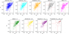 |
Fig. 13 Same as Fig. 12, but for maskcom.. |
| In the text | |
|
Fig. 14 Example of a source for which the HOG method indicates a low morphological correlation and the Spearman correlation indicates a high correlation. The source is AG019.8843-0.5337 and in the comparison of the continuum and of the moment-0 of H2CO 30,3−20,2 in the maskext. VN=0.20, while ρs = 0.67. The two panels in the upper row show the continuum and the moment-0 map of H2CO 30,3−20,2 with superimposed the directions of the gradients in the two maps (red: moment-0, white: continuum, respectively). The panel in the lower row shows the scatter plot of the pixel-to-pixel rank variables in the two maps inside the same mask (in black in the images of the two maps) where both the Spearman correlation and the Projected Rayleigh Statistic, VN, have been computed. |
| In the text | |
|
Fig. 15 Example of a source for which the HOG method indicates a high morphological correlation and the Spearman correlation coefficient indicates a low correlation. The source is AG332.7016-0.5870 and in the comparison of the continuum and of the moment-0 of H2CO 32,1−22,0 in the maskcom. VN=0.64, while ρs=0.07. The two panels in the upper row show the continuum and the moment-0 map of H2CO 32,1−22,0 with superimposed the directions of the gradients in the two maps (red: moment-0, white: continuum, respectively). The panel in the lower row shows the scatter plot of the pixel-to-pixel rank variables in the two maps inside the same mask (in black in the images of the two maps) where both the Spearman correlation and the Projected Rayleigh Statistic, VN, have been computed. |
| In the text | |
|
Fig. A.1 Figure illustrating the steps defining the masks used in this paper for source AG024.4616+0.1981 for the continuum and for the moment-0 of H2CO 30,3−20,2. Upper row: continuum maskcomp.; middle row: steps for the creation of continuum maskext.; bottom row first two panel from left: steps for the creation of the mask on moment-0; bottom row last two panel on the right: intersection masks used for the analysis. |
| In the text | |
|
Fig. B.1 Steps of the determination of the range of integration for the moment-0 maps for the example source AG024.4616+0.1981 for H2CO 3(0,3)-2(0,2) (top row) and CH3CN 120,1 − 110,1 (bottom row). Top row from left: 1) mean spectrum over all the pixel with peak emission above 4 S/N, with its best fit and derived range of integration in magenta; 2) pixel with highest peak spectrum, with its best fit and derived range of integration in green; 3) spectrum of the pixel with the blue-wing terminating at the lowest velocity, marked by the blue vertical line; 4) spectrum of the pixel with the red-wing terminating at the highest velocity, marked by the red vertical line. Bottom row: same as top row, but for CH3CN 120,1 − 110,1 for which a 2-Gaussian fit is performed to include both K=0 and K=1 line. No spectra are shown in the last two panel since no pixel was found with wings above the integration range defined by the first two panels. |
| In the text | |
|
Fig. C.1 Distribution of the VN parameter, calculated by astroHOG on pairs of noise-only moment-0 maps. |
| In the text | |
|
Fig. C.2 Gradients comparison on a pair of noise-only maps from Table C.1 for source AG023.0417+0.2925. The color scale units are Jy/beam km s−1 in both panels. The cyan lines indicate the direction of the gradients of the noise map in the left panel, while the red lines indicate the direction of the gradient of the noise map in the right panel. For this pair of noise maps VN is 0.013. |
| In the text | |
|
Fig. E.1 Top left panel: same of Fig. 9, that is, results of the astroHOG analysis on all the sample; top right panel: same plot only for the sources for which the automated routine for the creation of moment-0 maps failed; bottom panel: same plot excluding from all the sources those with a CORNISH counterpart. |
| In the text | |
Current usage metrics show cumulative count of Article Views (full-text article views including HTML views, PDF and ePub downloads, according to the available data) and Abstracts Views on Vision4Press platform.
Data correspond to usage on the plateform after 2015. The current usage metrics is available 48-96 hours after online publication and is updated daily on week days.
Initial download of the metrics may take a while.