| Issue |
A&A
Volume 692, December 2024
|
|
|---|---|---|
| Article Number | A55 | |
| Number of page(s) | 16 | |
| Section | Interstellar and circumstellar matter | |
| DOI | https://doi.org/10.1051/0004-6361/202450653 | |
| Published online | 02 December 2024 | |
PRODIGE – envelope to disk with NOEMA
IV. An infalling gas bridge surrounding two Class 0/I systems in L1448N
1
Max Planck Institute for Extraterrestrial Physics,
Gießenbachstraße 1,
85749
Garching bei München,
Germany
2
Department of Astronomy, The University of Texas at Austin,
2515 Speedway,
Austin,
TX
78712,
USA
3
Institut de Radioastronomie Millimétrique (IRAM),
300 rue de la Piscine,
38406
Saint-Martin d’Hères,
France
4
IPAG, Université Grenoble Alpes, CNRS,
38000
Grenoble,
France
5
Centre for Star and Planet Formation, Niels Bohr Institute, University of Copenhagen,
Øster Voldgade 5–7,
1350
Copenhagen,
Denmark
6
Max-Planck-Institut für Astronomie,
Königstuhl 17,
69117
Heidelberg,
Germany
7
SKA Observatory, Jodrell Bank,
Lower Withington,
Macclesfield
SK11 9FT,
UK
8
Centro de Astrobiología (CAB), CSIC-INTA,
Ctra.deTorrejón a Ajalvir km 4,
28806,
Torrejón de Ardoz,
Spain
★ Corresponding author; This email address is being protected from spambots. You need JavaScript enabled to view it.
Received:
8
May
2024
Accepted:
26
October
2024
Abstract
Context. The formation of stars has been subject to extensive studies in the past decades on scales from molecular clouds to proto-planetary disks. It is still not fully understood how the surrounding material in a protostellar system, which often shows asymmetric structures with complex kinematic properties, feeds the central protostar(s) and their disk(s).
Aims. We study the spatial morphology and kinematic properties of the molecular gas surrounding the IRS3A and IRS3B protostellar systems in the L1448N region located in the Perseus molecular cloud.
Methods. We present 1 mm Northern Extended Millimeter Array (NOEMA) observations of the large program PROtostars & DIsks: Global Evolution (PRODIGE). We analyzed the kinematic properties of molecular lines. Because the spectral profiles are complex, the lines were fit with up to three Gaussian velocity components. The clustering algorithm called density-based spatial clustering of applications with noise (DBSCAN) was used to disentangle the velocity components in the underlying physical structure.
Results. We discover an extended gas bridge (≈3000 au) surrounding both the IRS3A and IRS3B systems in six molecular line tracers (C18O, SO, DCN, H2CO, HC3N, and CH3OH). This gas bridge is oriented in the northeast-southwest direction and shows clear velocity gradients on the order of 100 km s−1 pc−1 toward the IRS3A system. We find that the observed velocity profile is consistent with analytical streamline models of gravitational infall toward IRS3A. The high-velocity C18O (2-1) emission toward IRS3A indicates a protostellar mass of ≈1.2 M⊙.
Conclusions. While high angular resolution continuum data often show IRS3A and IRS3B in isolation, molecular gas observations reveal that these systems are still embedded within a large-scale mass reservoir, whose spatial morphology and velocity profiles are complex. The kinematic properties of the extended gas bridge are consistent with gravitational infall toward the protostar IRS3A.
Key words: stars: formation / stars: protostars / ISM: kinematics and dynamics / ISM: individual objects: LDN 1448N
© The Authors 2024
 Open Access article, published by EDP Sciences, under the terms of the Creative Commons Attribution License (https://creativecommons.org/licenses/by/4.0), which permits unrestricted use, distribution, and reproduction in any medium, provided the original work is properly cited.
This article is published in open access under the Subscribe to Open model.
Open Access funding provided by Max Planck Society.
1 Introduction
Star formation is a hierarchical process from (giant) filamentary molecular clouds of up to several hundred parsec in size (Ragan et al. 2014) to protostellar cores with sizes <0.1 pc that harbor protostars (Pineda et al. 2023). The most embedded phase of low-mass star formation (with final stellar masses M✮ lower than ≈2 M⊙) is the Class 0/I stage, during which the protostellar systems are still embedded within their natal core envelope (Evans et al. 2009; Dunham et al. 2014).
Interferometric observations in the millimeter (mm) wavelength range with, for example, the Northern Extended Millimeter Array (NOEMA), the Submillimeter Array (SMA), and the Atacama Large Millimeter/submillimeter Array (ALMA), allow us to study nearby star-forming regions on scales of a few 1000 au to several au, which trace the cold gas and dust.
Surveys with a high angular resolution (≲0″. 3) have revealed structured planet-forming disks with a diversity of physical and chemical properties (e.g., Fedele et al. 2017; Andrews et al. 2018; Segura-Cox et al. 2020; Öberg et al. 2021; Ohashi et al. 2023; Miotello et al. 2023). Stars are often arranged in multiple systems (e.g., Offner et al. 2023), where the multiplicity fraction can be even higher in the early evolutionary phases (e.g., Tobin et al. 2016b).
Extended emission is often filtered out in interferometric observations, that is, the surrounding envelope material. Because the envelope can be the main mass reservoir, it is important to study star-forming regions on intermediate scales of a few 100 au to fill the gap between single-dish and interferometric observations. This regime is crucial for connecting the large-scale properties of the cloud, filament, and core with the characteristics of the protostar(s) and protoplanetary disks. In particular, it is important to trace the gas flows from filament and core scales to the protostars and disks. Protostellar envelopes have asymmetric and complex structures (e.g., Tobin et al. 2010, 2011, 2012; Maureira et al. 2017). The kinematic properties of the molecular gas surrounding protostars reveal asymmetric gas flows with infall motions that are sometimes referred to as streamers. These motions reach scales of a few 100 au to several 1000 au (e.g., Yen et al. 2014, 2017; Pineda et al. 2020; Ginski et al. 2021; Garufi et al. 2022; Valdivia-Mena et al. 2022; Hsieh et al. 2023; Fernández-López et al. 2023). These streamers can be traced by a variety of species, such as CS, DCN, HCO+ , H2CO, HC3N, CH3CN, and CH3OH, and their chemical properties and their connection to the natal environment is still subject of active research. While models of early protostel- lar gravitational collapse assumed that a spherically symmetric envelope forms a single protostar (e.g., Larson 1969; Shu 1977), more sophisticated models and simulations have been developed over the recent years in which multiple systems can form as well (Kuffmeier 2024, and references within). Analytic infall models assuming spherical symmetry can describe the kinematics of the asymmetric gas by tracing the kinematic profile of material along the streamlines (Pineda et al. 2020; Valdivia-Mena et al. 2022).
In this work, we study the kinematic properties of gas flows in the L1448N region, which is located in the Perseus molecular cloud at a distance of 288 pc (estimated by combining Gaia astrometry, stellar photometry, and CO maps, Zucker et al. 2018). We also study the connection of these flows to the embedded protostellar systems IRS3A and IRS3B. The left panel in Fig. 1 presents an overview of the cold dust distribution surrounding the L1448N region as traced by 850 µm continuum emission, taken from the Coordinated Molecular Probe Line Extinction and Thermal Emission (COMPLETE) survey (Ridge et al. 2006) with the James Clerk Maxwell Telescope (JCMT). A dense dust core toward L1448N harbors three protostellar systems: IRS3A, IRS3B, and IRS3C. The Class 0 protostar L1448-mm is located at a projected distance of ≈25 000 au toward the southeast.
The protostars in the Perseus molecular cloud have been studied extensively in the past by tracing both the large- and small-scale environment (e.g., Jørgensen et al. 2007, 2009). Within the Mass Assembly of Stellar Systems and their Evolution (MASSES) survey, envelope masses of 0.10 M⊙ and 0.34 M⊙ and outflow position angles (PA) of 218° and 122° were derived for IRS3A and IRS3B, respectively (Lee et al. 2016). The bolometric luminosity of IRS3A and IRS3B was estimated to be 9.2 ± 1.3 and 8.3 ± 0.8 L⊙, respectively (Tobin et al. 2016b). L1448N hosts at least six protostars: The VLA Nascent Disk and Multiplicity Survey of Perseus Protostars (VANDAM) revealed that IRS3A is a single protostar, IRS3C is a binary system, and IRS3B is a triple system (IRS3B-a, IRS3B-b, and IRS3B- c hereafter; marked in the right panel in Fig. 1) (Tobin et al. 2016b). While IRS3B-c dominates the mm emission, the close binary IRS3B-a and IRS3B-b dominates in mass (Tobin et al. 2016a). Moreover, about 1 arcmin away from L1448N, L1448- mm, which is also known as L1448C or Per-emb-26, lies part of a multiple system with the nearby L1448C(S) system, also known as Per-emb-42 (Jørgensen et al. 2006; Tobin et al. 2016b).
Several surveys have targeted these protostars to account for the chemical complexity in these regions. The survey Continuum And Lines in Young ProtoStellar Objects (CALYPSO) did not reveal any secure detections of complex organic molecules in IRS3A and IRS3B, except for a tentative detection of methanol (CH3 OH) and methyl formate (CH3OCHO) (De Simone et al. 2017; Belloche et al. 2020). In the survey Perseus ALMA Chemistry Survey (PEACHES), detections of CH3OH, CH3CN, CH3OCHO were reported toward IRS3A and IRS3B-c, but none toward IRS3B-a/b (Yang et al. 2021). Most notably, Yang et al. (2021) find that while for most of their sample, the emission of CH3OH that surrounds the protostars is compact, the emission for IRS3A is extended.
The orientations of known bipolar outflows are marked in Fig. 1. A large-scale outflow is launched by L1448-mm (e.g., Bally et al. 1993; Bachiller et al. 1995; Barsony et al. 1998; Jiménez-Serra et al. 2011), and the blueshifted lobe is directed toward L1448N. Toledano-Juárez et al. (2023) reported that the outflows in L1448-mm with a northwest-southeast direction interact with the close-by L1448-C(S) outflow. The redshifted lobes of both outflows are colliding with each other, but these authors found no evidence for triggered star formation. The midinfrared (MIR) study by O’Linger et al. (2006) revealed that only L1448-mm and L1448 IRS3A are bright in the mid-infrared (from 12.5 µm to 24.5 µm). By modeling the spectral energy distribution (SED) from the MIR to mm wavelengths, these authors reported for both IRS3A and L1448-mm systems two temperature components at ≈20 K and ≈90 K. The authors suggested that IRS3A is close to being a Class I system by comparing the envelope mass Menv = 0.29 M⊙ to Class 0 and I systems from the literature. The authors also concluded that the nondetection of the IRS3B system in the MIR might be related to the disruption of the IRS3A envelope by the L1448-mm outflow, while IRS3B is still embedded within its natal envelope.
Tobin et al. (2016a) and Reynolds et al. (2021) presented high angular resolution observations (≲0″.3) with ALMA that revealed spiral structures in the IRS3B disk (with a size of 497 au × 351 au). They also claimed this potentially for IRS3A. Reynolds et al. (2021) suggested that the triple system in IRS3B formed via disk fragmentation: IRS3B-a and IRS3B-b might have formed first, and the tertiary component IRS3B-c might have recently formed via gravitational instability. In contrast to this, Reynolds et al. (2021) found that the disk of IRS3A, with a size of 197 au × 72 au, is gravitationally stable. At a spatial resolution of 8 au, ALMA revealed that the IRS3A disk structure is a ring, and a fourth protostar might be embedded in the IRS3B disk (Reynolds et al. 2024).
In summary, the protostellar systems in L1448N have been substantially studied from IR to cm wavelengths, at which both the large-scale structures (> few thousand au) and the smallest scales down to the disks and protostars (< few dozen au) were targeted. However, important aspects for understanding the formation of these low-mass protostellar systems have not yet been addressed: The material flow onto the protostellar systems, and a possible connection to the larger-scale filament (Fig. 1 left panel) or to matter in between. The effect of the blueshifted outflow that is launched by L1448-mm on the L1448N region, and the possibility that this outflow may have triggered the formation of the systems in L1448N, as was suggested in the literature (e.g., Barsony et al. 1998; O’Linger et al. 2006).
A survey targeting these scales (300 au to few 1000 au) is the NOEMA large program PROtostars & DIsks: Global Evolution (PRODIGE). The PolyFiX correlator of NOEMA tuned to 1.4 mm wavelengths provides a broad bandwidth of 16 GHz, which allows us to simultaneously observe a plethora of molecular lines and obtain a sensitive continuum image. In total, 32 Class 0/I systems toward the Perseus molecular cloud are covered by the ongoing PRODIGE project, in which scales down to ≈300 au are resolved with an angular resolution of ≈1″. The first PRODIGE results of the program have revealed infalling streamers in H2CO in Per-emb-50 (Valdivia-Mena et al. 2022) and in DCN emission in the hot corino SVS13A (Hsieh et al. 2023, 2024). The second part of PRODIGE targeted eight Class II disks in Taurus. It revealed compact and extended disks in 12CO, 13CO, and C18O (2–1) line emission (Semenov et al. 2024). By modeling these species, disk gas masses between 0.005 and 0.04 M⊙ were determined (Franceschi et al. 2024). The PRODIGE program covers two NOEMA pointings toward IRS3A and IRS3B, as sketched by the dashed gray circles in Fig. 1.
In this work, we investigate the kinematic properties of the cold molecular gas in the L1448N region using molecular line observations with NOEMA toward the IRS3A and IRS3B systems and determine how they might be affected by the nearby protostellar systems IRS3C and L1448-mm. The paper is organized as follows: In Sect. 2, we explain the data-calibration procedure, including phase self-calibration, mosaic combination, and imaging of the NOEMA data. The analyses of the molecular line morphology and kinematic properties are presented in Sect. 3. Our findings are discussed in Sect. 4, and our conclusions are summarized in Sect. 5.
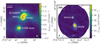 |
Fig. 1 Continuum images toward L1448N. The left panel shows the JCMT 850 µm emission taken from the COMPLETE survey in color (Ridge et al. 2006; Kirk et al. 2006). The dashed gray circles show the primary beam (22″.8) of the two NOEMA pointings of the PRODIGE observations. The protostellar systems of L1448N (IRS3A, IRS3B, and IRS3C) and the nearby L1448-mm system are marked by black squares. The beam of the JCMT and NOEMA observations is shown in the bottom right corner in green and black, respectively. In the right panel, we present the 1.4 mm continuum image of the PRODIGE observations in color and white contours. The contour levels are 5, 10, 20, 40, 80, and 160×σcont (σcont=0.94mJy beam−1). The black circles mark the positions of individual protostars taken from the VANDAM survey (Tobin et al. 2016b). The synthesized beam of the NOEMA data is shown in the bottom left corner. In both panels, scale bars are marked in the top left corner, and the bipolar outflow orientations are highlighted by red and blue arrows (Sect. 3.2). |
2 Observations
The NOEMA observations were obtained within the PRODIGE project (program id: L19MB, PIs: P. Caselli and Th. Henning). One part of PRODIGE targets 32 Class 0/I protostars in the Perseus molecular cloud in total, including two NOEMA single pointing observations centered on the IRS3A and IRS3B systems in L1448N (Fig. 1).
2.1 Single-pointing observations
Both IRS3A and IRS3B were observed with a single pointing each at 1.4 mm with a NOEMA primary beam of size 22″.8 (indicated by dashed circles in the left panel in Fig. 1). The phase centers (right ascension α and declination δ (J2000)) for the IRS3A and IRS3B pointings are 03h25m36.499s +30°45′21″.88 and 03h25m36.379s +30°45′14″.73, respectively. The observations in C and D configurations with 10 or 11 antennas in the array were taken from December 2019 to August 2021 and covered baselines from 16 m (12 kλ) to 370 m (272 kλ). These baseline ranges roughly correspond to spatial scales of 6000 au to 300 au at the distance of L1448N (288 pc, Zucker et al. 2018).
The PolyFiX correlator was set to a tuning frequency in the 1.4 mm range, covering frequencies from 214.7 GHz to 222.8 GHz in the lower sideband and from 230.2 GHz to 238.3 GHz in the upper sideband, with a channel width of 2MHz (≈2.6 km s−1). These are referred to as wideband data in the following. The wideband consists of four basebands covering ≈4 GHz each. Within the wideband frequency coverage, 39 high spectral resolution (narrowband) units were placed that targeted molecular lines at a higher spectral resolution of 62.5 kHz (≈0.09 km s−1).
The NOEMA data were calibrated using the continuum and line interferometer calibration (CLIC) package in GILDAS1. Bright radio sources (3C 84 or 3C 454.3) were used to calibrate the frequency bandpass. For amplitude and phase calibration, 0322+222 and 0333+321 were jointly observed every ≈20 minutes within each observation track. For the absolute flux calibration, we used LkHA 101, 2010+723 and/or MWC 349. With NOEMA, the flux calibration at 1.4 mm is correct at the 20% level or better.
The data were further processed with the MAPPING package of GILDAS. In each wideband baseband, a continuum- subtracted cube and a continuum image was created. The continuum was created with the uv_continuum task after carefully masking channel ranges at the edges of the baseband and with line emission using uv_filter. The same mask was applied for the continuum subtraction of the wideband cubes with the uv_baseline task fitting a first-order polynomial to visibilities in the continuum-only channels.
Atmospheric instabilities cause a high phase noise, but because the IRS3A and IRS3B systems are both bright sources at 1.4 mm, the dynamic range can be significantly increased by applying phase self-calibration after the standard calibration procedure (e.g., Gieser et al. 2021). We performed a phase self-calibration on the combined C- and D-configuration continuum data of each baseband separately, including all executions to obtain the highest signal-to-noise ratio (S/N), and we then applied the gain solutions to the corresponding wide- and narrowband data.
First, the continuum data were imaged with robust weighting (robust parameter 1) to maximize the spatial resolution, and they were then imaged with the Hogbom cleaning algorithm (Högbom 1974). A support mask was defined around the continuum sources. Self-calibration was performed in three loops, with decreasing integration times from 300 s, 135 s, to 45 s and a simultaneously increasing number of iterations (750, 1500, and 2000 and 500, 750, and 1500 for the IRS3A and IRS3B NOEMA pointing, respectively). We flagged visibilities with gain solutions whose S/N was lower than 6. For the IRS3A and IRS3B NOEMA data, 1% and 2% of the visibilities were flagged in the self-calibration step, respectively.
The gain solutions were applied to the wide- and narrowband data using the uv_cal task, where uncalibrated visibilities with S/N < 6 were flagged. We then subtracted the continuum from the narrowband units by first flagging channels at the edges of the unit and channel ranges containing line emission with uv_filter, and we then fit a zeroth- or first-order polynomial to continuum-only channel ranges, which we subtracted with the uv_baseline task.
Properties of the molecular lines covered by the NOEMA PRODIGE observations.
2.2 Mosaic combination
The phase centers of the two NOEMA pointings are only separated by 7″.2. The self-calibrated continuum and line data can therefore be combined into a mosaic. Because IRS3A and IRS3B have slightly different velocities (5.3 km s−1 and 4.7 km s−1, respectively), we adopted an intermediate source velocity of 5 km s−1 for the mosaic. For individual line cubes, the velocity was set to the line center using the modify command, and a subcube was extracted around the line using uv_extract. To combine both pointings, the spectral axis was placed on the same grid using the uv_resample task. In order to increase the S/N, all line cubes were rebinned to a common resolution of 0.1 km s−1. For the observed CO and SiO transitions, the width of the narrowband units did not cover the full extent of the line emission because of the broad outflow line wings. We thus also extracted wideband cubes for these two lines, rebinned to a channel width of 3.0 km s−1. We then combined the two NOEMA pointings for the continuum and line data into a mosaic using the uv_mosaic task. The phase center was set as the center between the two NOEMA pointings, with α=03h25m36.439s and δ=+30°45′ 18″.7304 (J2000).
The mosaic continuum data were cleaned with a robust weighting (robust parameter of 1) with the Hogbom algorithm and a support mask down to three times the theoretical noise. A manually defined support mask covered the IRS3A and IRS3B continuum sources. The mosaic line data were cleaned with natural weighting to increase the line S/N and the Hogbom algorithm down to the theoretical noise. For the DCN (3–2), HC3N (24– 23), and CH3OH (42,3−31,2E) line cubes, we defined a support mask in each channel that contained significant line emission or absorption. For both the mosaic continuum and line data, we applied primary beam correction.
The morphology in the continuum images in the four basebands is similar. The intensity increases with frequency, as expected from cold dust emission. We thus only present the continuum image created from the lower inner baseband, centered at 220.785 GHz (1.4 mm), as shown in the right panel in Fig. 1. The synthesized beam has a size of 0′90×0′73 (PA=18°), and the continuum noise σcont is 0.94 mJy beam−1.
The properties of the molecular line transitions we analyzed are summarized in Table 1. With the applied natural weighting, the synthesized beam with a size of ≈1.″2 × 0.″9 is slightly larger than the continuum data. We estimated the line noise per channel in the central area of the mosaic in line-free channel ranges. The line noise σline is ≈0.2K in the high spectral resolution (δv = 0.1 km s−1) data, and it is ≈0.04K in the low spectral resolution (δv = 3.0 km s−1) data.
3 Results
The 1.4 mm L1448N continuum map of the PRODIGE observations is presented in the right panel in Fig. 1. The IRS3A and IRS3B systems are both clearly resolved in their cold dust emission. We also mark the positions of individual protostars detected by the VANDAM survey (Tobin et al. 2016b). With an angular resolution of ≈1″ (300 au), the three protostars in IRS3B (labeled a, b, and c) are not resolved. We can only distinguish between the outer IRS3B-c protostar and the IRS3B-ab binary system. Nevertheless, the PRODIGE observations allowed us to study the spatial morphology and kinematic properties of the molecular gas that surrounds the IRS3A and IRS3B systems on scales of a few hundred to a few thousand au.
3.1 Spatial morphology of the molecular gas
With the PRODIGE data, common abundant molecular species are detected in the L1448N region. The detected lines we analyzed and their properties are summarized in Table 1. Unlike the hot-corino source SVS13A, for which the PRODIGE data show a plethora of transitions by complex organic molecules (Hsieh et al. 2023, 2024), CH3 OH is the most complex species detected with NOEMA at the sensitivity and angular resolution in L1448N. In particular, for each molecule, only one transition is detected. It is therefore not possible to reliably derive excitation temperatures and column densities.
To investigate the spatial morphology, we computed line- integrated intensity (moment 0) maps of all molecular lines listed in Table 1. For each transition, we integrated along all velocities that contained line emission:  . The last two columns in Table 1 summarize the velocity ranges, vlow and vupp , we used for each transition to compute the moment 0 map. This means that depending on the tracer, the velocity ranges can be larger (e.g., for CO with broad line wings due to the presence of molecular outflows) than for the lines with narrow line widths around the source velocity. For CO and SiO, whose line wings are broader than the extent of the narrowband units, we used the wideband line data to compute the integrated-intensity maps. The integrated-intensity maps are presented in Fig. 2 for all nine molecular lines presented in this work. Figure A.12 shows spectra of all transitions extracted from the IRS3A and IRS3B continuum peak position.
The moment 0 map of CO (2–1) shows extended emission within the full field of view (FoV). The emission traces bipolar outflows from the IRS3A and IRS3B systems, as well as from the nearby IRS3C and L1448-mm systems, which are outside the FoV of the NOEMA mosaic (Fig. 1). With a shortest baseline of 16 m, spatial scales larger than ≈22″ (6600 au) are filtered out during the observations. Missing flux due to this filtering is most prominent in CO with negative artifacts. SiO (5–4) emits brightly and surrounds the IRS3B system east and west. It traces shocks along the bipolar outflow and south of IRS3B. No extended SiO emission is detected toward IRS3A above 3σline. In Sect. 3.2, we further analyze the observed outflows by studying the red- and blueshifted line wings of the CO and SiO emission.
The OCS (18–17) line has compact emission around the IRS3A and IRS3B protostars. It traces warmer gas with Eu/kB ≈ 100 K. Although the angular resolution of the NOEMA observations is insufficient for resolving the triple system within the IRS3B system, the OCS emission clearly peaks at the position of the IRS3B-c protostar, which is located in the outer part of the disk. The integrated-intensity map of SO (65−54) also shows bright emission peaks toward IRS3A, while for IRS3B, the emission peaks in between of the protostars in the triple system. SO is also detected east of IRS3B in the redshifted part of the outflow. The emission southwest toward the edge of the FoV can be linked to gas that is shocked by the L1448-mm outflow (further discussed in Sect. 3.2). In addition, there is faint SO emission in between the IRS3A and IRS3B systems.
The extended emission surrounding the IRS3A and IRS3B systems is prominent in C18O (2−1), H2CO (30,3 − 20,2), DCN (3−2), HC3N (24−23), and CH3OH (42,3 − 31,2E). We refer to this feature as the “bridge” in the following, and its extent is highlighted by the pink polygon in the bottom panels in Fig. 2. This bridge extends from north of IRS3A to the IRS3B disk, it embeds these two systems, and has a filamentary substructure. Toward the IRS3B disk, DCN is highly absorbed against the bright continuum emission. In addition to the bridge, the H2CO moment 0 map traces the IRS3B outflow. The C18O and H2CO integrated-intensity maps show negative features due to the spatial filtering, suggesting that the gas bridge might be even more extended. However, the emission of DCN, HC3N, and CH3OH is compact enough, and the missing flux filtered out by the interferometric observations is not substantial.
The morphology of the extended molecular emission suggests that this gas bridge connects the IRS3A system to the IRS3B disk. A similar gas bridge has been found toward the Class 0 system IRAS16293-2422 (Pineda et al. 2012; van der Wiel et al. 2019). It was concluded by van der Wiel et al. (2019) that this quiescent bridge is remnant filamentary material from the natal protostellar envelope. The gas bridge in L1448N might be associated with the outflows, or it might have a different origin. In order to investigate the properties of this bridge that is revealed in the PRODIGE molecular line data, we first study the outflow morphology of IRS3A and IRS3B (Sect. 3.2), and in Sect. 3.4, we perform a kinematic analysis of the gas bridge.
3.2 Molecular outflows in L1448N
The identification of the outflow orientations of protostars in the L1448N region in early studies was difficult (e.g., Bachiller et al. 1990, 1995; Bally et al. 1993; Barsony et al. 1998) because of the close by L1448-mm outflow, which has a bright and extended southeast (redshifted)–northwest (blueshifted) orientation, as indicated in Fig. 1. Infrared observations also revealed multiple large-scale outflows originating in the L1448N region (e.g., Tobin et al. 2007).
The emission of CO (2−1) and SiO (5−4) of the PRODIGE data clearly reveals bipolar outflows in L1448N (Fig. 2). To distinguish the red- and blueshifted parts of the outflows, we computed the line-integrated intensity of the redshifted, central, and blueshifted velocity ranges for both transitions. For CO, we analyzed both the low- and high-velocity components with the narrowband and wideband data, respectively. The top row in Fig. 3 shows the outflow morphology for CO (low- and high- velocity components in the left and middle panel, respectively) and SiO (right panel). The red- and blueshifted integrated intensities are highlighted by red and blue contours, respectively. The contour levels are 10, 30, 50, and 90% of the peak-integrated intensity. We checked for all maps that the 10% level is higher than five times the integrated-intensity noise, σmom0. This was calculated as  , where nchannels is the number of channels used to compute the corresponding integrated-intensity map, and σline and δv are the line noise per channel and the channel width, respectively (Table 1). The velocity ranges are shown in the top left corner in each panel in Fig. 3 and are highlighted by dashed vertical red and blue lines in the spectra presented in the bottom panels in Fig. 3.
The IRS3A protostar launches a northeast (blueshifted)- southwest (redshifted) outflow that is detected in CO (2–1) without a counterpart in SiO (5–4). The redshifted outflow lobe of IRS3A is only present close to the source velocity (up to vLSR + 6 km s−1; shown in color scale and thus not visible in the red contours). This indicates that the outflow is inclined close the plane of the sky.
The redshifted emission in low-velocity CO from northwest in the FoV down to the southeast can mistakenly be identified as the outflow from IRS3A because it overlaps with the source. However, it is launched by the IRS3C system, which is located northwest of IRS3A, but outside of the FoV of the mosaic.
The IRS3B system launches a southeast (redshifted)- northwest (blueshifted) outflow with shocked high-velocity bullets of CO and SiO along both outflow lobes. The bottom panels of Fig. 3 show example spectra for CO and SiO. The high- velocity SiO bullets extent up to ±50 km s−1 from the source velocity.
The blueshifted emission in the east and south seen in both CO and SiO are associated with the large-scale outflow of the L1448-mm protostar. In Fig. B.1 we show the outflow morphology of the low-velocity component of CO in L1448N as well as L1448-mm, which was also observed within the PRODIGE project. The blueshifted emission blob in the northwest is also most likely associated with this outflow (as suggested by Girart & Acord 2001) because it was found that the outflow lobe is asymmetric and bent toward the northwest at the location of L1448N (e.g., Froebrich et al. 2002; Hirano et al. 2010; Yoshida et al. 2021). A detailed analysis of the PRODIGE observations of the L1448-mm outflow will be presented in a different publication. The blueshifted CO emission in the low-velocity regime might also partially be caused by foreground cloud emission.
All systems in L1448N show bipolar outflows. The projected size of the IRS3A outflow is small (<1000 au), while the CO outflow of IRS3B traces a wide-angle outflow cavity that extends well beyond the FoV. While the IRS3A outflow has no counterpart in SiO, toward the IRS3B outflow, SiO traces shocked high-velocity bullets that suggest energetic episodic outbursts (Vorobyov et al. 2018).
In the MASSES survey, Lee et al. (2016) reported an outflow PA of 218 ± 10° and 122 ± 15° for IRS3A and IRS3B, respectively. These outflow orientations are orthogonal with respect to the disks, with a PA of 133° and 28°, respectively (Reynolds et al. 2021). From the observed CO outflow lobes (Fig. 3), we estimate an outflow PA of 225° and 99° for IRS3A and IRS3B, respectively. For IRS3A, the outflow PA is consistent with the findings from Lee et al. (2016).
For IRS3B, the outflow PA derived from the PRODIGE high- velocity CO data (99°) is consistent with the high-velocity SiO bullets shown in the right panel in Fig. 3. Toward the southeast of IRS3B, a wide-angle cavity is detected in CO close to the source velocity, however. Our results are consistent with the high-velocity SiO bullets launched by IRS3B-c revealed by ALMA (Reynolds et al. 2021), while the wide-angle outflow with a PA of 120–130° (Lee et al. 2016; Dunham et al. 2024) is associated with the compact IRS3B-ab system.
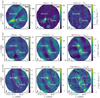 |
Fig. 2 Line-integrated intensity maps of the PRODIGE observations. The line-integrated intensity and the 1.4 mm continuum are presented in color and white contours, respectively. The contour levels are 5, 40, and 160×σcont (σcont=0.94mJybeam−1). The IRS3A and IRS3B protostellar systems toward L1448N are labeled in white. The black circles mark the positions of individual protostars taken from the VANDAM survey (Tobin et al. 2016b). The bipolar outflow orientations are indicated by blue and red arrows. The synthesized beam of the line and continuum data is indicated in the bottom left and bottom right corner, respectively. A scale bar is shown in the top right corner. In the bottom row panels, the extent of the bridge structure is indicated by the dashed pink polygon. The spectra toward the continuum peak position of IRS3A and IRS3B are shown in Fig. A.1 for all transitions. |
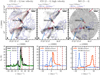 |
Fig. 3 Molecular outflows in L1448N. The red and blue contours in the top panels show the red- and blueshifted line-integrated intensities of low-velocity CO 2–1 (left), high-velocity CO 2–1 (center), and SiO 5–4 (right). The contour levels are 0.1, 0.3, 0.5, and 0.9× the corresponding peak-integrated intensity. We present the integrated intensity around the source velocity in color. The integration ranges are listed in each panel and are indicated by dashed vertical red and blue lines in the spectra in the bottom panels. The outflow orientations are indicated by blue and red arrows. The black contours are the 1.4 mm continuum of the PRODIGE observations. The contour levels are 5, 10, 20, 40, 80, and 160×σcont (σcont=0.94mJy beam−1). The protostellar systems of the L1448N system (IRS3A and IRS3B) are labeled in black. The synthesized beam of the line and continuum data is indicated in the bottom left and bottom right corner, respectively. A scale bar is shown in the top right corner. The bottom panels show spectra that were extracted from the positions indicated by the black triangles in the top panels. The vertical dashed gray line is the region velocity of L1448N (≈5 km s−1). |
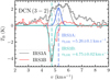 |
Fig. 4 Spectrum of DCN (3–2) toward the continuum peak position of IRS3A (black) and IRS3B (red). A Gaussian fit to the central velocities is shown in blue and green, and the source velocities are indicated by vertical dashed lines for IRS3A and IRS3B, respectively. In the case of IRS3A, three components were fit in total to account for the complexity of the spectrum. The central velocity components correspond to the blue line, and the additional two components are highlighted by the dash- dotted gray lines. The total three-component fit is indicated by the solid gray line. |
3.3 Source velocity and mass estimates
We used the DCN (3–2) transition to estimate the individual source velocities of IRS3A and IRS3B. The spectra of DCN (3–2) extracted from the continuum peak position of IRS3A and IRS3B are shown in Fig. 4 in black and red, respectively. The high spectral resolution of the PRODIGE data (0.1 km s−1) reveals a complex line profile toward IRS3A. Multiple high- velocity components lie in the red- and blueshifted ranges. Based on the IRS3A spectrum, we estimate the source velocity to be 5.26 ± 0.10 km s−1 from a three-component Gaussian model fit toward the central velocity component. This source velocity is consistent with the results from a position-velocity (PV) diagram of C18O (2−1) (5.2 km s−1, as analyzed in the following) and Reynolds et al. (2021, 5.4 km s−1). The IRS3A spectrum shows multiple velocity components, and the kinematic properties with a multicomponent fit are further analyzed in Sect. 3.4.
The DCN (3–2) spectrum toward the continuum peak of IRS3B shows strong absorption, which can be explained by the high optical depth of the disk continuum emission and/or foreground DCN with a lower excitation temperature than the continuum. High continuum opacities commonly cause absorption features of molecular lines (e.g., Ohashi et al. 2022; Codella et al. 2024; Podio et al. 2024). We estimate a source velocity of 4.75±0.02 km s−1 for IRS3B, which is consistent with Reynolds etal. (2021, 4.8 km s−1).
The DCN (3–2) emission and absorption toward the continuum peak position of IRS3A and IRS3B, respectively, already reveal multiple underlying physical components that cause emission or absorption at various velocities. In Sect. 3.4, we disentangle the complex line profiles by fitting multiple Gaussian velocity components to DCN (3–2) as well as HC3N (24–23) and CH3OH (42,3−31,2E) to derive the kinematic structure in the entire region, with a focus on the gas bridge.
The mass of a (proto)star is the most important property that influences its evolution strongly, but it is not straightforward to measure the protostellar mass of the central objects. Reynolds et al. (2021) estimated the mass of the IRS3B system by obtaining a PV diagram of C17O (3−2) emission: for the IRS3B-ab binary, they derived a mass of 1.15 M⊙, and for IRS3B-c, they derived an upper limit of 0.2 M⊙. These authors were not able to reliably fit the PV diagram of IRS3A and estimated a value of 1.4 M⊙ by a visual inspection. In addition, they estimated the IRS3A mass to be 1.5 ± 0.1 M⊙ based on a radiative transfer modeling of the SO2 line emission.
We used the C18O (2–1) transition of the PRODIGE data to estimate the protostellar mass of IRS3A. For IRS3B, the contribution of the extended envelope and the gas bridge is too high in C18O emission in order to reliably estimate the kinematic mass. Young embedded disks around Class 0/I protostars are warm enough to prevent CO freeze-out compared to isolated Class II disks (van’t Hoff et al. 2020). The radiative transfer models by Tobin et al. (2020) showed that the average disk temperature is ≈60 K and ≈70 K for protostellar luminosities of 1 L⊙ and 10 L⊙, respectively. Thus, C18O is expected to be in the gas phase in the entire disk of the embedded Class 0/I IRS3A system with L = 9.2 L⊙ (Tobin et al. 2016b).
We used the pvextractor package (Ginsburg et al. 2015, 2016) to extract a PV diagram of C18O (2–1) along the orientation of the disk (133±1°, Reynolds et al. 2021) with a width of 1″. The PV diagram is shown in color in Fig. 5, whereas 4, 8, and 16σline levels are indicated by black contours (σline = 0.22 K). In order to estimate the mass, we used the KeplerFit Python package (Bosco et al. 2019, 2023) to fit the observed PV diagram with models assuming Keplerian disk rotation. A good estimate of the mass, with uncertainties of about a few 10%, can be obtained by fitting the edge of the emission (Seifried et al. 2016; Bosco et al. 2019; Ahmadi et al. 2023). In our case, we fit the 4σline contour level of the emission in the PV diagram. It should be noted, however, that marginally resolved data can cause an overestimate of the mass due to a broadening along the velocity axis (e.g., Maret et al. 2020). Ohashi et al. (2023) compared the mass of R CrA IRS7B-a derived with the PV diagram method using the edge method as well as the ridge method. They reported differences of ≈1 M⊙.
The best-fit Keplerian disk model is indicated by a dashed red line in Fig. 5. We only included ranges in radius that are highlighted by the solid red line that included bright line emission. We mostly focused on the redshifted part of the emission since the blueshifted part missed flux in some parts. The final mass was corrected for the inclination of the disk (69°, Reynolds et al. 2021). We assumed an uncertainty of 5° for the disk inclination. We obtained a mass of 1.2±0.1 M⊙, where the uncertainty includes the errors from the fit as well as the uncertainty of the inclination. This value agrees within the uncertainties with the mass reported by Reynolds et al. (2021, 1.4 M⊙). The source velocity from the best-fit Keplerian model was estimated to be 5.2 km s−1, which agrees with the estimate based on the DCN (3−2) transition (Fig. 4).
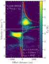 |
Fig. 5 Position-velocity diagram of C18O (2–1) toward IRS3A extracted along the orientation of the disk with a width of 1″. The black contours highlight levels at 4, 8, and 16×σline (σline = 0.22 K, Table 1). The best- fit derived by KeplerFit is shown as a dashed red line. The ranges in radius that are included in the fit are indicated by the solid red line. |
3.4 Kinematic structure of the gas bridge in L1448N
The line-integrated intensity maps (Fig. 2) reveal an extended gas bridge in L1448N that surrounds the IRS3A and IRS3B systems and in which they are embedded. The outflow orientations of the systems are known (Sect. 3.2). We were therefore able to study the gas bridge and its kinematic properties. This gas bridge might be associated with the outflow or might have a different origin, for example, infalling material. We analyzed the kinematic properties of the gas bridge using the DCN (3−2), HC3N (24–23), and CH3OH (42,3−31,2E) transitions (bottom row in Fig. 2) because these molecules trace the bridge without contamination from the outflows and because the emission is compact enough so that no flux is missing. A zoom-in on the integrated intensity map of these three molecules and example spectra of these three transitions at selected positions along the gas bridge is presented in Fig. 6.
The high spectral resolution of the PRODIGE data (0.1 km s−1) spectrally resolves the line profiles well and reveals multiple velocity components as well as clear velocity gradients along the gas bridge. Thus, we first fit up to three Gaussian velocity components to the DCN, HC3N, and CH3 OH line data (Sect. 3.4.1) and then applied a clustering algorithm to disentangle the velocity components (Sect. 3.4.2).
3.4.1 Gaussian decomposition of the spectral line profiles
The kinematic properties, with a focus on the peak velocity of the different velocity components, were analyzed using the pyspeckit python package and its specfit function (Ginsburg & Mirocha 2011; Ginsburg et al. 2022). We fit up to one, two, and three Gaussian velocity components (nGauss,max) to the HC3N, CH3 OH, and DCN spectra, respectively. Each Gaussian component was defined by three parameters (peak amplitude Ipeak , velocity v, and standard deviation σGauss). The corresponding full width at half maximum (FWHM) line width corresponds to  .
.
First, we created a noise map for each transition by estimating the noise in each pixel in line-free channel ranges. Then, the spectrum in each pixel was evaluated, and when the S/N was higher than 5 within a velocity range of 3 km s−1 and 7 km s−1, the spectrum was fed into pyspeckit. We only analyzed the area that is covered by the gas bridge, as highlighted by the dashed gray ellipse in Fig. 6. A single Gaussian component (peak amplitude Ipeak, velocity 3, and standard deviation σGauss) was then fit to the observed spectrum using the specfit function with use_lmfit = True. In the case of the HC3N (24−23) transition, no significant residuals were present in the spectra in a fit with one Gaussian velocity component.
In a next step, for DCN and CH3 OH, a second Gaussian velocity component was fit to the data. This procedure was repeated for DCN because the velocity profile of DCN (3−2) shows areas that are clearly dominated by three velocity components (Fig. 6). In Fig. C.1, we present example spectra as well as the best fit from the Gaussian decomposition at some positions along the gas bridge (Fig. 6).
To avoid overfitting as well as discard unreliable fits, we applied a quality assessment of the results. We discarded all velocity components with σGauss < 0.07 km s−1 (corresponding to Δv = 0.16 km s−1) for all three transitions. They are associated to unreliable narrow fits in noisy spectra. For DCN and CH3OH, we computed the Akaike information criterion (AIC) for the one-, two- and (in the case of DCN) three-component fit (AIC1 , AIC2, and AIC3, respectively) in order to select the best model fit. The AIC considers the least χ2 statistics as well as the number of free parameters in each model (see Appendix B in Valdivia-Mena et al. 2022). The best model has the lowest AIC value, AICmin , but only when it improves the AIC value by a difference of ΔAIC = 5 at least. The median uncertainty of the FWHM line width is 0.09, 0.07, and 0.11 km s−1 for the DCN, HC3N, and CH3 OH results, respectively.
Because the velocity components are complex and overlap spatially, it is not straightforward to assign the velocity components to their underlying physical structure. In the next section, we therefore use a clustering algorithm to disentangle the velocity components.
3.4.2 Clustering of the velocity components
We used the density-based spatial clustering algorithm DBSCAN of the scikit-learn Python package (Grisel et al. 2023) to cluster the velocity components for each transition (DCN, HC3N, and CH3OH). We aimed to recover the kinematic signature of the gas bridge.
Each cluster derived by DBSCAN consists of central core points as well as nearby neighborhood points. The clustering with DBSCAN is set by two parameters: the maximum distance between two data points for one to be considered as in the neighborhood of the other, eps, and the minimum number of data points in a cluster, minsamples. With DBSCAN, some data points may not be associated with any cluster, and we refer to them as discarded data points. The input parameters for DBSCAN are summarized in Table C.1 for each of the three transitions.
The input for DBSCAN is a list of data points that each consists of the 2D position and velocity (x, y, v). The peak intensity and line width are not given as an input, but we also analyzed the spatial distribution of these parameters of all velocity clusters to confirm that DBSCAN provided reasonable results. To further minimize the effect of outliers, the data set was scaled using the RobustScaler function of scikit-learn. This function removes the median and scales the data according to the quantile range between the first and third quantile. Then we ran DBSCAN for each molecule on this scaled data set. The output of DBSCAN is the number of clusters, as well as a list of data points (x, y, v) for each cluster. Data points that could not be associated with any cluster according to the defined parameters (eps and minsamples) were discarded.
The results from DBSCAN are summarized in Table C.1, and Fig. 7 shows the velocity map of each cluster for DCN, while the results for HC3N and CH3OH are presented in Fig. C.2. for DCN, a minor fraction of pixels after the clustering contains two velocity components. In these cases, the average values of the fit parameters (velocity, peak amplitude, and line width) were calculated. The peak amplitude and line width maps of the clusters of all three transitions are presented in Figs. C.3 and C.4, respectively.
For the DCN 3–2 transition (Fig. 7), we found four velocity clusters with DBSCAN. Cluster 1 traces the emission around the IRS3B disk at the source velocity of ≈4.7 km s−1. Clusters 2, 3, and 4 reveal the extended gas bridge and a red- (cluster 2 and 4) and blueshifted (cluster 3) part (in the east and west, respectively). At either side of the bridge, the velocities increase toward IRS3A with respect to the source velocity of ≈5.2 km s−1. In Sect. 4.1.1 we further discuss the velocity gradients of the bridge. Most notably, the envelope and disk rotation of IRS3A (as revealed by C17O 3–2, Reynolds et al. 2021) shows the same velocity pattern as the gas bridge (redshifted east of IRS3A, and blueshifted west of IRS3A). With the angular resolution of the PRODIGE data (300 au), we cannot resolve the IRS3A disk with a size of ≈100 au. High angular molecular line observations are therefore required to better study how the bridge structure is connected to the IRS3A disk.
Four clusters are found with DBSCAN for HC3N 24–23 (top panel in Fig. C.2). Clusters 1 and 4 can be associated with the blue- and redshifted part of the gas bridge, while clusters 2 and 3 trace the red- and blueshifted emission of the envelope and disk rotation of IRS3A. The HC3N emission is much less extended than DCN (3–2). The upper energy level of 131 K for HC3N (Table 1) is relatively high, which may mean that the emission traces warmer locations along the gas bridge as well as in the envelope and disk region.
For the CH3OH 42,3−31,2E transition, we find four velocity clusters with DBSCAN. Clusters 1 and 2 can be associated with envelope rotation of IRS3B. The velocity pattern roughly matches the C17O (3–2) envelope rotation found by Reynolds et al. (2021). We only detect CH3OH emission toward the outer edges of the disk. The nondetection toward the bright continuum disk location most likely arises because the high optical depth of the continuum blocks the line emission (e.g., De Simone et al. 2020). Clusters 3 and 4 can be associated with the blue- and redshifted part of the gas bridge, respectively.
In the right panels in Figs. 7 and C.2, we present the velocity maps of the discarded data. The separation in both position and velocity is small. Together with the spatial resolution of the PRODIGE data, it is challenging to disentangle the velocity components close to the IRS3A envelope and disk system as well as the spatial intersection of the red- and blueshifted part of the gas bridge.
The amplitude Ipeak and FWHM line width ∆v maps of all clusters derived with the three species are presented in Figs. C.3 and C.4, respectively. The smooth maps of the peak intensity and line width, both of which were no input parameters for the clustering, confirm that the clustering of the velocity data points with DBSCAN provides reliable results.
In the DCN (3–2) transition, the line widths along the gas bridge are narrow and ≈1 km s−1 or smaller, but they increase toward the location of the unresolved IRS3A disk. The line width of CH3 OH along the bridge is as narrow as DCN and HC3N, which means that the emission is most likely not caused by shocks. In order to disentangle the region close to the IRS3A protostar and its disk, line observations at higher angular resolution are necessary.
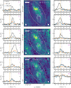 |
Fig. 6 Overview of the gas bridge. In the central panels, a zoom-in of the integrated-intensity maps (Fig. 2) is shown in color (top: DCN 3–2, middle: HC3N 24–23, and bottom: CH3OH 42,3 −31,2 E). The synthesized beam of the line and continuum data is shown in the bottom left and right corners, respectively. A scale bar is presented in the top left corner. The dashed gray ellipse shows the area that is covered by the gas bridge in which the kinematic analysis was conducted. We label the positions for which spectra are shown in the left and right panels in pink (black: DCN 3–2, orange: HC3N 24–23, and blue: CH3OH 42,3 − 31,2 E). The dashed vertical gray and orange lines indicate the source velocity of IRS3A and IRS3B, respectively. |
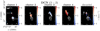 |
Fig. 7 Velocity clusters derived with DBSCAN for DCN (3–2). The velocity of a cluster is shown in each panel in color, and the discarded data points are shown in the last panel. The 1.4 mm continuum data are presented in white contours, and the levels are 5, 10, 20, 40, 80, and 160×σcont (σcont=0.94mJy beam−1). In the first panel, the outflow directions are indicated and the sources are marked. A scale bar of 1000au is shown in the top left corner. The synthesized beam of the line and continuum data is shown in the bottom left and right panels, respectively. The velocity clusters for HC3N and CH3 OH are presented in Fig. C.2. The corresponding amplitude Ipeak and FWHM line width ∆3 of all three transitions are presented in Figs. C.3 and C.4, respectively. |
4 Discussion
We have revealed an extended gas bridge between IRS3A and IRS3B with the PRODIGE molecular line data of IRS3A and IRS3B. These two protostellar systems are located in L1448N. We disentangled the velocity components in the spectra to extract the kinematic signature of the gas bridge in the molecular tracers DCN (3–2), HC3N (24–23), and CH3OH (42,3−31,2E) in Sect. 3.4. We found that the gas bridge consists of a redshifted side that extends east and a blueshifted side that extends west of the IRS3A and IRS3B systems. In the following, we discuss the properties of the gas bridge, that is, the velocity gradients and infalling motions, the impact of the infall, and possible origins of the gas bridge.
4.1 Infall motions along the gas bridge
4.1.1 Velocity gradients
To study velocity gradients at either side of the gas bridge, we used the velocity gradient code used by Pineda et al. (2010) that is available in the velocity_tools3 Python package. The velocity maps of the red- and blueshifted parts of the gas bridge already show velocity gradients along its major axis (Figs. 7 and C.2). Whereas the difference in velocity is only about a few 0.1 km s−1 , which highlights the necessity for a high spectral resolution, this difference occurs over small spatial scales, on the order of a few 1000 au. We computed the velocity gradient using the velocity maps of the two sides of the gas bridge derived with DBSCAN (Sect. 3.4.2). The results for DCN (3–2) are shown in Fig. 8, and the results for HC3N (24–23) and CH3OH (42,3−31,2E) are shown in Figs. C.5 and C.6, respectively. The velocity gradient results for the red- and blueshifted part of the gas bridge are shown in the top and bottom panels in Fig. 8, respectively. The left panel shows the velocity map overlaid with purple arrows that highlight the direction and strength of the velocity gradient, the middle panel shows the velocity gradient map, and the right panel is a map of the PA of the velocity gradient.
The velocity gradient of the gas bridge is on the order of a few 10 km s−1 pc−1 to ≈120 km s−1 pc−1 for DCN (3–2). For both parts of the gas bridge, the velocities become more extreme toward IRS3A, that is, more redshifted and blueshifted. This suggests infalling motions from both parts of the gas bridge toward IRS3A. In the next section, we apply a streamline model to both sides of the gas bridge to determine whether gravitational infall caused by the IRS3A protostar can explain the observed velocities along the gas bridge. The southern part of the redshifted gas bridge indicates velocity gradients toward IRS3B as well, which can also be clearly seen in the change in the PA of the gradient near IRS3B (top right panel in Fig. 8). More sensitive and higher angular resolution observations are required in order to investigate a potential connection of the gas bridge with the IRS3A and IRS3B disks.
Even though the velocity maps of HC3N and CH3OH are less extended than DCN (3–2), the redshifted side of the gas bridge shows a similar morphology in velocity as DCN (Figs. C.5 and C.6). The bottom part of the blueshifted side of the gas bridge in CH3OH shows an additional east-west gradient in the direction of IRS3B. While the gas bridge shows increasing velocity gradients toward IRS3A, there might be infall toward IRS3B as well.
Notably, the rotation of the IRS3A envelope and disk system (Reynolds et al. 2021) occurs in a similar direction, that is, west (blueshifted) to east (redshifted). This is a strong indication that the gas bridge is a remnant structure of the common elongated filament out of which the IRS3A and IRS3B systems have formed. We further discuss the origin of the gas bridge in Sect. 4.3.
The overall, that is, global, velocity gradient for each side and molecular tracer of the gas bridge is summarized in Table C.1. We find global velocity gradients in the range of 50–120 km s−1 pc−1 and 70–130 km s−1 pc−1 for the redshifted and blueshifted side of the gas bridge, respectively. These values are consistent with the velocity gradients found by Gupta et al. (2022, 70 km s−1 pc−1 and 120 km s−1 pc−1 for IRS3A and IRS3B, respectively), who studied the velocity gradients using C180 (2−1). One explanation for the differences in the two sides might be the unknown inclination of the gas bridge. In the scenario of the infalling gas bridge, a high-velocity gradient could cause strong accretion events in the IRS3A disk and might explain why IRS3A is much brighter in the IR than IRS3B (O’Linger et al. 2006). In contrast to this gas bridge around IRS3A and IRS3B, the gas bridge toward IRAS 16293 – 2422 is quiescent, and no strong velocity gradients are detected in C170 (3−2) (van der Wiel et al. 2019).
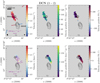 |
Fig. 8 Velocity gradient maps of the red- (top) and blueshifted (bottom) part of the gas bridge. In each row, the velocity (left), velocity gradient (center), and velocity gradient PA (right) are shown in color. The black contours are the 1.4 mm continuum with levels at 5, 10, 20, 40, 80, and 160×σcont (σcont=0.94mJybeam−1). The purple arrows in the left panels indicate the direction and strength of the velocity gradient, where the arrow tip points from low to high velocities. The length of the purple arrow in the bottom left corner marks a velocity gradient of 100 km s−1pc−1. In the top left panel, the synthesized beam of the NOEMA line and continuum data are shown in the bottom left and right corner, respectively. A scale bar is shown in the top left corner, and bipolar outflow orientations are highlighted by red and blue arrows (Sect. 3.2). |
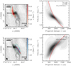 |
Fig. 9 Streamline model of the red- (top) and blueshifted (bottom) sides of the gas bridge. The left panel shows the integrated intensity of DCN (3−2) in grayscale and the velocity map in color. The black contours are the 1.4 mm continuum with levels at 5, 10, 20, 40, 80, and 160×σcont (σcont=0.94 mJy beam−1). The synthesized beam of the NOEMA line and continuum data is shown in the bottom left and right panels, respectively. A scale bar is shown in the top left corner. The right panel shows the kernel density estimate of the observed velocity profile in grayscale as a function of projected distance and the streamline model in red. The projected trajectory of the streamline model is highlighted in red in the left panels as well. The position at which the streamline model reaches the centrifugal radius is marked by the red triangle. |
4.1.2 Streamline model
To investigate whether the observed velocity gradients along the two sides of the gas bridge can be explained by gravitational infall due to the central IRS3A protostar, we used the streamline model by Pineda et al. (2020). The model uses an analytic solution of a free-falling accretion flow of a rotating parcel toward a central gravitating object assuming conservation of angular momentum (Mendoza et al. 2009). We applied the model to the observed DCN (3−2) velocities of the red- and blueshifted side (clusters 4 and 3, respectively) of the gas bridge derived in Sect. 3.4.2.
The streamline model computed the position and velocity of a test mass along the streamline. The coordinate system was set such that the ɀ-axis pointed along the angular momentum vector of the disk, and the x- and y-axis corresponded to the disk plane. For both streamline models, we used an inclination i of 21° (Reynolds et al. 2021) and position angle of 225° (Sect. 3.2) to set the orientation of the angular momentum vector of the disk. The protostellar mass was 1.2 M⊙, and the source velocity was set to 5.26 km s−1, as derived in Sect. 3.3.
The accretion flow is described by its initial position (r0, θ0, ϕ0) and initial radial velocity vr0. Due to our limited FoV set by the primary beam, we set r0 = 2500 au for both sides of the gas bridge, which matches the extent of the observed gas bridge structure. The initial rotation of the parcel is described by Ω0, which we estimated by the difference of peak velocity of the gas bridge with respect to the source velocity, that is, ≈0.5 km s−1, and the length of the streamer,  . The corresponding centrifugal radius is rcentr = 1200 au. The streamline model computed the position and velocity from r0 up until rcentr.
We explored the parameter space of the remaining three parameters − θ0, ϕ0, and vr0 , and searched manually by eye for streamline models that reproduce the projected trajectory as well as the velocity profile. The left panels in Fig. 9 show the integrated intensity of DCN (3−2) in grayscale and the red- and blueshifted velocity side of the gas bridge overlaid in color in the top and bottom panels, respectively. The right panels shows the corresponding kernel density estimate of the observed velocity profile in grayscale. In the left panels, we show the projected trajectory and in the right panels the velocity profile of the best-fit streamline model. For the redshifted side of the gas bridge, we obtain a good match for θ0 = 145°, ϕ0 = 240°, and vr0 = 0.3 km s−1, and for the blueshifted side of the gas bridge, we obtain a good match for θ0 = 15°, ϕ0 = 65°, and vr0 = 0.0 km s−1.
For the two sides of the gas bridge, we found solutions of the streamline model that matched the observed trajectory as well as velocity profile. This means that the observed velocity gradients might be caused by the gravitational pull of the central IRS3A protostar. The streamline model does not include the assumption of conservation of angular momentum, which limits the model. Moreover, no interaction with the surrounding envelope material was considered. The impact of the infalling material is further discussed in Sect. 4.2.
4.2 Impact of the gas bridge on the IRS3A and IRS3B disks
We found that the gas bridge is connected to the rotation envelope and disk of IRS3A with infalling motions. There is evidence that the bridge is also partially connected to the IRS3B disks, but data with a higher angular resolution are required to disentangle the kinematically complex region. The PRODIGE data at a resolution of 1″ (≈300 au) cannot spatially resolve the IRS3A disk, and observations with a higher angular resolution are therefore necessary to resolve the impact of the gas bridge on the disk. Compact emission of shock-tracing species such as SO and OCS is bright toward the position of the IRS3A disk (Fig. 2). Asymmetric SO emission has been attributed to a streamer impact toward Per-emb-50 within the PRODIGE data (Valdivia-Mena et al. 2022).
Ring-like and spiral arm structures are evident in the disks of IRS3A and IRS3B, respectively (Reynolds et al. 2021, 2024). Gravitational instabilities could have been triggered through the infalling material of the gas bridge, as suggested by simulations (e.g., Kuffmeier et al. 2018). Comparing our large-scale observations with the high angular resolution ALMA observations by Reynolds et al. (2021), we find indications of a connection of the gas bridge with the IRS3A disk in H13CO+ and SO2 emission (their Figs. 8 and 10, respectively). These two transitions shows the same red- and blueshifted morphology of the gas bridge in the east and west, respectively, as are observed in DCN, HC3N, and CH3OH. The integrated intensity of CS 5−4 from the ALMA PEACHES survey also shows the redshifted side of the gas bridge and was interpreted as an infalling envelope (Artur de la Villarmois et al. 2023), while in the maps of IRS3B, the CS emission follows the bipolar outflow. Observations with a high spatial resolution in the mm regime of shock-tracing molecules might together with sensitive MIR observations of hydrogen-recombination lines with the James Webb Space Telescope (JWST) also reveal accretions shocks in the IRS3A disk (Rigliaco et al. 2015).
4.3 Possible origins of the gas bridge
A kinematic analysis of the PRODIGE molecular line data revealed that the gas bridge is infalling toward IRS3A from the two sides of the gas bridge (Sect. 4.1). A sketch of the infall and outflow motions is presented in Fig. 10. In the following, we discuss potential explanations of the bridge structure formation.
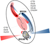 |
Fig. 10 Sketch of the kinematic components of the gas bridge as well as bipolar outflows surrounding the IRS3A and IRS3B protostellar systems in L1448N. The grayscale images show the 1.3 mm emission with ALMA, taken from the VANDAM survey (Tobin et al. 2018). Individual protostars are highlighted with yellow stars. |
4.3.1 Molecular outflow of IRS3A
The orientation of the gas bridge is parallel to the orientation of the bipolar outflow from IRS3A. However, the spatial morphology and kinematic properties of CO that trace the outflow are different from the gas bridge that is traced in DCN, HC3N, and CH3OH. The line widths of these tracers are narrow (<2 km s−1, Fig. C.4) and are thus likely not caused by shocks from the IRS3A outflow. We therefore rule out that the gas bridge is a signature of a rotating outflow, as was suggested for other pro-tostars with rotating outflows (e.g., Zapata et al. 2015; Bjerkeli et al. 2016; Tabone et al. 2017; Zhang et al. 2018; Oya et al. 2021; Nazari et al. 2024).
4.3.2 Remnant filamentary material
Another explanation might be that the gas bridge is remnant material from the natal envelope structure from which the IRS3A and IRS3B systems formed. SMA observations (whose primary beam is 2.5× larger than that of NOEMA at 1.4 mm) of the MASSES survey revealed an extended N-S filament that connects IRS3A and IRS3B in 13CO (2−1), C18O (2−1), as well as HCO+ (4−3) emission (Lee et al. 2015, their Fig. 5). The IRS3A and IRS3B systems might accrete material from this filament. While O’Linger et al. (2006) claimed that IRS3A is IR-bright (S12.5 µm = 0.43 Jy compared to S12.5 µm < 0.12 Jy for IRS3B) because it has already dispersed the surrounding material, the results by Lee et al. (2015) and our PRODIGE data reveal that both IRS3A and IRS3B are still embedded within filamentary material (Fig. 2). The high IR brightness of IRS3A can be explained by the fact that it is accreting from the gas bridge (Sect. 4.1.2), which produces a high accretion luminosity. Numerical simulations of low-mass star-forming regions commonly show that protostars in multiple systems are surrounded by filamentary gas structures (e.g., Kratter et al. 2010; Kuffmeier et al. 2018, 2019; Lee et al. 2019).
Simulations by Kuffmeier et al. (2019) revealed that bridge structures (with sizes of 103–104 au) connect protostars that formed as a result of compressive flows in turbulent environments. Protostars accrete material from the bridge that feeds the disks. In the simulations, the bridge structures are transient objects that last a few 10 kyr and are connected to the larger-scale filament. In addition, turbulent fragmentation causes the formation of protostellar companions with separations of ≈1000 au. Comparing these simulations with the observed properties of the IRS3A and IRS3B systems, we suggest that the close binary system IRS3B-a/b might have formed from disk fragmentation (e.g., Kratter et al. 2010), whereas the tertiary component may have formed later through turbulent fragmentation (e.g., Offner et al. 2010) of the gas bridge and migrated toward the IRS3B-a/b system. The simulated gas bridge by Kuffmeier et al. (2019) could provide material toward multiple protostars, and in the case of the L1448N system, both the IRS3A and IRS3B-c protostars might still strongly accrete from the gas bridge. An analysis of the stability of the IRS3B disk suggests that the IRS3B-c protostar might have also formed via disk fragmentation, however (Tobin et al. 2016a; Reynolds et al. 2021). Higher angular resolution observations of molecular lines toward IRS3B are necessary to study the impact of the gas bridge on the disk.
4.3.3 Triggered star formation
L1448N is located in northwest of L1448-mm (Fig. 1), and the blueshifted outflow-lobe of L1448-mm is not only oriented along L1448N, but blueshifted emission knots from CO, SO, H2CO, and CH3OH are detected in the PRODIGE FoV (Fig. 2). It was already hypothesized by Barsony et al. (1998) that L1448-mm might have triggered the formation of the L1448N systems. Because the redshifted lobe of the IRS3C outflow impacts the L1448 IRS3A and IRS3B systems as well (Fig. 3), the material from the L1448-mm and IRS3C systems might have affected the material around IRS3A and IRS3B from both sides. The impact of the outflows might have shocked and compressed the filament toward IRS3A and IRS3B, while in the surroundings, cold material that is evident in N2H+ emission is spatially offset from the filament that connects IRS3A and IRS3B (Lee et al. 2015). Observations with a high angular resolution in the MIR, together with JWST targeted heated and/or shocked material, are necessary to follow up on this. Spitzer and Herschel observations show bright IR emission from atomic and molecular lines such as H2, FeII, SI, and OI that originate from the L1448-mm outflow (Neufeld et al. 2009; Nisini et al. 2013, 2015). However, the spatial resolution is not sufficient to disentangle the different protostellar systems within L1448N, but the L1448-mm outflow might still have influenced or even triggered the formation of protostars in L1448N. To further investigate this, a better determination of the L1448-mm outflow timescale with respect to the lifetimes of the protostellar systems in L1448N is necessary.
The protostellar systems in L1448N are surrounded by nearby systems with large-scale outflows. The molecular gas in L1448N shows complex kinematic properties. Extended gas is revealed in a bridge structure surrounding IRS3A, and IRS3B is most likely connected to the filamentary structure from which these systems have formed. However, the L1448-mm outflow as well as the outflows of IRS3A might also have affected the formation of the bridge structure.
5 Conclusions
NOEMA 1 mm observations of the PRODIGE project toward L1448N revealed extended molecular emission in the structure of a gas bridge that surrounds the IRS3A and IRS3B proto-stellar systems. We analyzed the spatial morphology as well as the kinematic properties of spectral lines in several molecular tracers, such as DCN, HC3N, and CH3OH.
The PRODIGE data reveal that the IRS3A and IRS3B systems are embedded in extended molecular gas that extends well beyond the FoV of the observed mosaic (>6600au). An elongated gas bridge with bright emission connects the IRS3A and IRS3B protostellar systems. This is most evident in C18O, H2CO, DCN, HC3N, and CH3OH;
Using a Keplerian disk rotation model applied to the observed PV diagram of C18O, we were able to determine the central mass of IRS3A to be 1.2±0.1 M⊙. This value agrees with radiative transfer modeling results by Reynolds et al. (2021), who estimated the mass to be 1.5 ± 0.1 M⊙;
The high spectral resolution data with a channel width of 0.1 km s−1 revealed complex dynamics, including multiple velocity components along the line of sight. For DCN, HC3N, and CH3OH, individual velocity components were extracted with a multicomponent Gaussian fitting. By applying the DBSCAN clustering algorithm, we associated these velocity components with envelope and disk rotation of the protostellar systems and with a red- and blueshifted side of the gas bridge;
Velocity gradients along the gas bridge revealed infalling material toward IRS3A from both the red- and blueshifted sides. Locally, the velocity gradients rise to 120 km s−1 pc−1, while the global average is ≈100 km s−1 pc−1. We applied a streamline model to the observed velocity profiles of the two sides of the gas bridge and confirmed that the observations are consistent with gravitational infall toward IRS3A;
Both IRS3A and IRS3B launch bipolar outflows, as revealed by CO emission. The IRS3B outflow is also detected in high-velocity CO and SiO bullets. Within the observed FoV, a contribution from the nearby L1448-mm and IRS3C outflows is also detected (blueshifted and redshifted lobe, respectively). It has been suggested that the L1448-mm outflow might influence the IRS3A and IRS3B systems. We indeed found that bright SiO emission, hence shocked locations, are caused by L1448-mm toward L1448N.
Very high angular resolution observations often filter out extended emission. In L1448N, which harbors the IRS3A and IRS3B systems, we revealed extended molecular emission surrounds the two systems with NOEMA 1.3mm observations. The kinematic properties of the extended gas bridge are complex, and we found that the most likely explanation for the origin of the structure is that it is the remnant filament material out of which the IRS3A and IRS3B systems formed. To study the full extent of the gas bridge, a larger area needs to be covered in follow-up observations. At the same time, to reveal the impact zone of the gas bridge on the IRS3A and IRS3B disks, more spectral line observations at higher angular resolution and sensitivity are required. Nevertheless, the PRODIGE data highlight the importance of studying the extended, often infalling, material that surrounds protostellar systems on scales of a few 100 au.
Data availability
Appendices A, B, and C are available on Zenodo: https://doi.org/10.5281/zenodo.14001971.
Acknowledgements
We thank the referee John Tobin for his constructive feedback that substantially improved the paper. The authors thank the IRAM staff at the NOEMA observatory for their support in the observations and data calibration. This work is based on observations carried out under project number L19MB with the IRAM NOEMA Interferometer. IRAM is supported by INSU/CNRS (France), MPG (Germany) and IGN (Spain). DSC is supported by an NSF Astronomy and Astrophysics Postdoctoral Fellowship under award AST-2102405. D. S. and Th. H. acknowledge support from the European Research Council under the Horizon 2020 Framework Program via the ERC Advanced Grant Origins 832428 (PI: Th. Henning). I.J-.S acknowledges funding from grants PID2022-136814NB-I00 funded by MICIU/AEI/ 10.13039/501100011033 and by “ERDF/EU”.
References
- Ahmadi, A., Beuther, H., Bosco, F., et al. 2023, A&A, 677, A171 [NASA ADS] [CrossRef] [EDP Sciences] [Google Scholar]
- Andrews, S. M., Huang, J., Pérez, L. M., et al. 2018, ApJ, 869, L41 [NASA ADS] [CrossRef] [Google Scholar]
- Artur de la Villarmois, E., Guzmán, V. V., Yang, Y. L., Zhang, Y., & Sakai, N. 2023, A&A, 678, A124 [NASA ADS] [CrossRef] [EDP Sciences] [Google Scholar]
- Bachiller, R., Cernicharo, J., Martin-Pintado, J., Tafalla, M., &Lazareff, B. 1990, A&A, 231, 174 [NASA ADS] [Google Scholar]
- Bachiller, R., Guilloteau, S., Dutrey, A., Planesas, P., & Martin-Pintado, J. 1995, A&A, 299, 857 [NASA ADS] [Google Scholar]
- Bally, J., Lada, E. A., & Lane, A. P. 1993, ApJ, 418, 322 [CrossRef] [Google Scholar]
- Barsony, M., Ward-Thompson, D., André, P., & O’Linger, J. 1998, ApJ, 509, 733 [NASA ADS] [CrossRef] [Google Scholar]
- Belloche, A., Maury, A. J., Maret, S., et al. 2020, A&A, 635, A198 [NASA ADS] [CrossRef] [EDP Sciences] [Google Scholar]
- Bjerkeli, P., van der Wiel, M. H. D., Harsono, D., Ramsey, J. P., & Jørgensen, J. K. 2016, Nature, 540, 406 [Google Scholar]
- Bosco, F., Beuther, H., Ahmadi, A., et al. 2019, A&A, 629, A10 [NASA ADS] [CrossRef] [EDP Sciences] [Google Scholar]
- Bosco, F., Beuther, H., Ahmadi, A., et al. 2023, KeplerFit: Keplerian velocity distribution model fitter, Astrophysics Source Code Library [record ascl:2308.012] [Google Scholar]
- Codella, C., Podio, L., De Simone, M., et al. 2024, MNRAS, 528, 7383 [NASA ADS] [CrossRef] [Google Scholar]
- De Simone, M., Codella, C., Testi, L., et al. 2017, A&A, 599, A121 [NASA ADS] [CrossRef] [EDP Sciences] [Google Scholar]
- De Simone, M., Ceccarelli, C., Codella, C., et al. 2020, ApJ, 896, L3 [NASA ADS] [CrossRef] [Google Scholar]
- Dunham, M. M., Stutz, A. M., Allen, L. E., et al. 2014, in Protostars and Planets VI, eds. H. Beuther, R. S. Klessen, C. P. Dullemond, & T. Henning, 195 [Google Scholar]
- Dunham, M. M., Stephens, I. W., Myers, P. C., et al. 2024, MNRAS, 533, 3828 [NASA ADS] [CrossRef] [Google Scholar]
- Evans, Neal J., I., Dunham, M. M., Jørgensen, J. K., et al. 2009, ApJS, 181, 321 [NASA ADS] [CrossRef] [Google Scholar]
- Fedele, D., Carney, M., Hogerheijde, M. R., et al. 2017, A&A, 600, A72 [NASA ADS] [CrossRef] [EDP Sciences] [Google Scholar]
- Fernández-López, M., Girart, J. M., López-Vázquez, J. A., et al. 2023, ApJ, 956, 82 [CrossRef] [Google Scholar]
- Franceschi, R., Henning, T., Smirnov-Pinchukov, G. V., et al. 2024, A&A, 687, A174 [NASA ADS] [CrossRef] [EDP Sciences] [Google Scholar]
- Froebrich, D., Smith, M. D., & Eislöffel, J. 2002, A&A, 385, 239 [NASA ADS] [CrossRef] [EDP Sciences] [Google Scholar]
- Garufi, A., Podio, L., Codella, C., et al. 2022, A&A, 658, A104 [CrossRef] [EDP Sciences] [Google Scholar]
- Gieser, C., Beuther, H., Semenov, D., et al. 2021, A&A, 648, A66 [EDP Sciences] [Google Scholar]
- Ginsburg, A., & Mirocha, J. 2011, PySpecKit: Python Spectroscopic Toolkit, Astrophysics Source Code Library [record ascl:1109.001] [Google Scholar]
- Ginsburg, A., Robitaille, T., Beaumont, C., et al. 2015, in Astronomical Society of the Pacific Conference Series, 499, Revolution in Astronomy with ALMA: The Third Year, eds. D. Iono, K. Tatematsu, A. Wootten, & L. Testi, 363 [Google Scholar]
- Ginsburg, A., Robitaille, T., & Beaumont, C. 2016, pvextractor: Position-Velocity Diagram Extractor, Astrophysics Source Code Library [record ascl:1608.010] [Google Scholar]
- Ginsburg, A., Sokolov, V., de Val-Borro, M., et al. 2022, AJ, 163, 291 [NASA ADS] [CrossRef] [Google Scholar]
- Ginski, C., Facchini, S., Huang, J., et al. 2021, ApJ, 908, L25 [NASA ADS] [CrossRef] [Google Scholar]
- Girart, J. M., & Acord, J. M. P. 2001, ApJ, 552, L63 [CrossRef] [Google Scholar]
- Grisel, O., Mueller, A., Lars, et al. 2023, scikit-learn/scikit-learn: Scikit-learn 1.3.2, https://zenodo.org/records/13749328 [Google Scholar]
- Gupta, A., Yen, H.-W., Koch, P., et al. 2022, ApJ, 930, 67 [NASA ADS] [CrossRef] [Google Scholar]
- Hirano, N., Ho, P. P. T., Liu, S.-Y., et al. 2010, ApJ, 717, 58 [NASA ADS] [CrossRef] [Google Scholar]
- Högbom, J. A. 1974, A&AS, 15, 417 [Google Scholar]
- Hsieh, T. H., Segura-Cox, D. M., Pineda, J. E., et al. 2023, A&A, 669, A137 [NASA ADS] [CrossRef] [EDP Sciences] [Google Scholar]
- Hsieh, T. H., Pineda, J. E., Segura-Cox, D. M., et al. 2024, A&A, 686, A289 [NASA ADS] [CrossRef] [EDP Sciences] [Google Scholar]
- Jiménez-Serra, I., Martín-Pintado, J., Winters, J. M., Rodríguez-Franco, A., & Caselli, P. 2011, ApJ, 739, 80 [CrossRef] [Google Scholar]
- Jørgensen, J. K., Harvey, P. M., Evans, Neal J., I., et al. 2006, ApJ, 645, 1246 [Google Scholar]
- Jørgensen, J. K., Bourke, T. L., Myers, P. C., et al. 2007, ApJ, 659, 479 [Google Scholar]
- Jørgensen, J. K., van Dishoeck, E. F., Visser, R., et al. 2009, A&A, 507, 861 [NASA ADS] [CrossRef] [EDP Sciences] [Google Scholar]
- Kirk, H., Johnstone, D., & Di Francesco, J. 2006, ApJ, 646, 1009 [Google Scholar]
- Kratter, K. M., Matzner, C. D., Krumholz, M. R., & Klein, R. I. 2010, ApJ, 708, 1585 [NASA ADS] [CrossRef] [Google Scholar]
- Kuffmeier, M. 2024, Front. Astron. Space Sci., 11, 1403075 [NASA ADS] [CrossRef] [Google Scholar]
- Kuffmeier, M., Frimann, S., Jensen, S. S., & Haugbølle, T. 2018, MNRAS, 475, 2642 [NASA ADS] [CrossRef] [Google Scholar]
- Kuffmeier, M., Calcutt, H., & Kristensen, L. E. 2019, A&A, 628, A112 [NASA ADS] [CrossRef] [EDP Sciences] [Google Scholar]
- Larson, R. B. 1969, MNRAS, 145, 271 [Google Scholar]
- Lee, K. I., Dunham, M. M., Myers, P. C., et al. 2016, ApJ, 820, L2 [NASA ADS] [CrossRef] [Google Scholar]
- Lee, K. I., Dunham, M. M., Myers, P. C., et al. 2015, ApJ, 814, 114 [CrossRef] [Google Scholar]
- Lee, A. T., Offner, S. S. R., Kratter, K. M., Smullen, R. A., & Li, P. S. 2019, ApJ, 887, 232 [NASA ADS] [CrossRef] [Google Scholar]
- Maret, S., Maury, A. J., Belloche, A., et al. 2020, A&A, 635, A15 [NASA ADS] [CrossRef] [EDP Sciences] [Google Scholar]
- Maureira, M. J., Arce, H. G., Offner, S. S. R., et al. 2017, ApJ, 849, 89 [NASA ADS] [CrossRef] [Google Scholar]
- Mendoza, S., Tejeda, E., & Nagel, E. 2009, MNRAS, 393, 579 [NASA ADS] [CrossRef] [Google Scholar]
- Miotello, A., Kamp, I., Birnstiel, T., Cleeves, L. C., & Kataoka, A. 2023, in Astronomical Society of the Pacific Conference Series, 534, Protostars and Planets VII, eds. S. Inutsuka, Y. Aikawa, T. Muto, K. Tomida, & M. Tamura, 501 [Google Scholar]
- Müller, H. S. P., Schlöder, F., Stutzki, J., & Winnewisser, G. 2005, J. Mol. Struct., 742, 215 [Google Scholar]
- Nazari, P., Tabone, B., Ahmadi, A., et al. 2024, A&A, 686, A201 [NASA ADS] [CrossRef] [EDP Sciences] [Google Scholar]
- Neufeld, D. A., Nisini, B., Giannini, T., et al. 2009, ApJ, 706, 170 [NASA ADS] [CrossRef] [Google Scholar]
- Nisini, B., Santangelo, G., Antoniucci, S., et al. 2013, A&A, 549, A16 [NASA ADS] [CrossRef] [EDP Sciences] [Google Scholar]
- Nisini, B., Santangelo, G., Giannini, T., et al. 2015, ApJ, 801, 121 [NASA ADS] [CrossRef] [Google Scholar]
- Öberg, K. I., Guzmán, V. V., Walsh, C., et al. 2021, ApJS, 257, 1 [CrossRef] [Google Scholar]
- Offner, S. S. R., Kratter, K. M., Matzner, C. D., Krumholz, M. R., & Klein, R. I. 2010, ApJ, 725, 1485 [Google Scholar]
- Offner, S. S. R., Moe, M., Kratter, K. M., et al. 2023, in Astronomical Society of the Pacific Conference Series, 534, eds. S. Inutsuka, Y. Aikawa, T. Muto, K. Tomida, & M. Tamura, 275 [NASA ADS] [Google Scholar]
- Ohashi, S., Codella, C., Sakai, N., et al. 2022, ApJ, 927, 54 [NASA ADS] [CrossRef] [Google Scholar]
- Ohashi, N., Tobin, J. J., Jørgensen, J. K., et al. 2023, ApJ, 951, 8 [NASA ADS] [CrossRef] [Google Scholar]
- O’Linger, J. C., Cole, D. M., Ressler, M. E., & Wolf-Chase, G. 2006, AJ, 131, 2601 [CrossRef] [Google Scholar]
- Oya, Y., Watanabe, Y., López-Sepulcre, A., et al. 2021, ApJ, 921, 12 [NASA ADS] [CrossRef] [Google Scholar]
- Pickett, H. M., Poynter, R. L., Cohen, E. A., et al. 1998, J. Quant. Spec. Radiat. Transf., 60, 883 [Google Scholar]
- Pineda, J. E., Goodman, A. A., Arce, H. G., et al. 2010, ApJ, 712, L116 [Google Scholar]
- Pineda, J. E., Maury, A. J., Fuller, G. A., et al. 2012, A&A, 544, L7 [NASA ADS] [CrossRef] [EDP Sciences] [Google Scholar]
- Pineda, J. E., Segura-Cox, D., Caselli, P., et al. 2020, Nat. Astron., 4, 1158 [NASA ADS] [CrossRef] [Google Scholar]
- Pineda, J. E., Arzoumanian, D., Andre, P., et al. 2023, in Astronomical Society of the Pacific Conference Series, 534, eds. S. Inutsuka, Y. Aikawa, T. Muto, K. Tomida, & M. Tamura, 233 [NASA ADS] [Google Scholar]
- Podio, L., Ceccarelli, C., Codella, C., et al. 2024, A&A, 688, L22 [NASA ADS] [CrossRef] [EDP Sciences] [Google Scholar]
- Ragan, S. E., Henning, T., Tackenberg, J., et al. 2014, A&A, 568, A73 [NASA ADS] [CrossRef] [EDP Sciences] [Google Scholar]
- Reynolds, N. K., Tobin, J. J., Sheehan, P., et al. 2021, ApJ, 907, L10 [NASA ADS] [CrossRef] [Google Scholar]
- Reynolds, N. K., Tobin, J. J., Sheehan, P. D., et al. 2024, ApJ, 963, 164 [Google Scholar]
- Ridge, N. A., Di Francesco, J., Kirk, H., et al. 2006, AJ, 131, 2921 [Google Scholar]
- Rigliaco, E., Pascucci, I., Duchene, G., et al. 2015, ApJ, 801, 31 [Google Scholar]
- Segura-Cox, D. M., Schmiedeke, A., Pineda, J. E., et al. 2020, Nature, 586, 228 [NASA ADS] [CrossRef] [Google Scholar]
- Seifried, D., Sánchez-Monge, Á., Walch, S., & Banerjee, R. 2016, MNRAS, 459, 1892 [NASA ADS] [CrossRef] [Google Scholar]
- Semenov, D., Henning, T., Guilloteau, S., et al. 2024, A&A, 685, A126 [NASA ADS] [CrossRef] [EDP Sciences] [Google Scholar]
- Shu, F. H. 1977, ApJ, 214, 488 [Google Scholar]
- Tabone, B., Cabrit, S., Bianchi, E., et al. 2017, A&A, 607, L6 [NASA ADS] [CrossRef] [EDP Sciences] [Google Scholar]
- Tobin, J. J., Looney, L. W., Mundy, L. G., Kwon, W., & Hamidouche, M. 2007, ApJ, 659, 1404 [NASA ADS] [CrossRef] [Google Scholar]
- Tobin, J. J., Hartmann, L., Looney, L. W., & Chiang, H.-F. 2010, ApJ, 712, 1010 [CrossRef] [Google Scholar]
- Tobin, J. J., Hartmann, L., Chiang, H.-F., et al. 2011, ApJ, 740, 45 [NASA ADS] [CrossRef] [Google Scholar]
- Tobin, J. J., Hartmann, L., Bergin, E., et al. 2012, ApJ, 748, 16 [Google Scholar]
- Tobin, J. J., Kratter, K. M., Persson, M. V., et al. 2016a, Nature, 538, 483 [NASA ADS] [CrossRef] [Google Scholar]
- Tobin, J. J., Looney, L. W., Li, Z.-Y., et al. 2016b, ApJ, 818, 73 [CrossRef] [Google Scholar]
- Tobin, J. J., Looney, L. W., Li, Z.-Y., et al. 2018, ApJ, 867, 43 [CrossRef] [Google Scholar]
- Tobin, J. J., Sheehan, P. D., Megeath, S. T., et al. 2020, ApJ, 890, 130 [CrossRef] [Google Scholar]
- Toledano-Juárez, I., de la Fuente, E., Trinidad, M. A., Tafoya, D., & Nigoche-Netro, A. 2023, MNRAS, 522, 1591 [CrossRef] [Google Scholar]
- Valdivia-Mena, M. T., Pineda, J. E., Segura-Cox, D. M., et al. 2022, A&A, 667, A12 [NASA ADS] [CrossRef] [EDP Sciences] [Google Scholar]
- van der Wiel, M. H. D., Jacobsen, S. K., Jørgensen, J. K., et al. 2019, A&A, 626, A93 [NASA ADS] [CrossRef] [EDP Sciences] [Google Scholar]
- van’t Hoff, M. L. R., Harsono, D., Tobin, J. J., et al. 2020, ApJ, 901, 166 [Google Scholar]
- Vorobyov, E. I., Elbakyan, V. G., Plunkett, A. L., et al. 2018, A&A, 613, A18 [NASA ADS] [CrossRef] [EDP Sciences] [Google Scholar]
- Yang, Y.-L., Sakai, N., Zhang, Y., et al. 2021, ApJ, 910, 20 [Google Scholar]
- Yen, H.-W., Takakuwa, S., Ohashi, N., et al. 2014, ApJ, 793, 1 [NASA ADS] [CrossRef] [Google Scholar]
- Yen, H.-W., Takakuwa, S., Chu, Y.-H., et al. 2017, A&A, 608, A134 [NASA ADS] [CrossRef] [EDP Sciences] [Google Scholar]
- Yoshida, T., Hsieh, T.-H., Hirano, N., & Aso, Y. 2021, ApJ, 906, 112 [CrossRef] [Google Scholar]
- Zapata, L. A., Lizano, S., Rodriguez, L. F., et al. 2015, ApJ, 798, 131 [NASA ADS] [CrossRef] [Google Scholar]
- Zhang, Y., Higuchi, A. E., Sakai, N., et al. 2018, ApJ, 864, 76 [NASA ADS] [CrossRef] [Google Scholar]
- Zucker, C., Schlafly, E. F., Speagle, J. S., et al. 2018, ApJ, 869, 83 [NASA ADS] [CrossRef] [Google Scholar]
All appendices are available on Zenodo: https://doi.org/10.5281/zenodo.14001971
All Tables
All Figures
|
Fig. 1 Continuum images toward L1448N. The left panel shows the JCMT 850 µm emission taken from the COMPLETE survey in color (Ridge et al. 2006; Kirk et al. 2006). The dashed gray circles show the primary beam (22″.8) of the two NOEMA pointings of the PRODIGE observations. The protostellar systems of L1448N (IRS3A, IRS3B, and IRS3C) and the nearby L1448-mm system are marked by black squares. The beam of the JCMT and NOEMA observations is shown in the bottom right corner in green and black, respectively. In the right panel, we present the 1.4 mm continuum image of the PRODIGE observations in color and white contours. The contour levels are 5, 10, 20, 40, 80, and 160×σcont (σcont=0.94mJy beam−1). The black circles mark the positions of individual protostars taken from the VANDAM survey (Tobin et al. 2016b). The synthesized beam of the NOEMA data is shown in the bottom left corner. In both panels, scale bars are marked in the top left corner, and the bipolar outflow orientations are highlighted by red and blue arrows (Sect. 3.2). |
| In the text | |
|
Fig. 2 Line-integrated intensity maps of the PRODIGE observations. The line-integrated intensity and the 1.4 mm continuum are presented in color and white contours, respectively. The contour levels are 5, 40, and 160×σcont (σcont=0.94mJybeam−1). The IRS3A and IRS3B protostellar systems toward L1448N are labeled in white. The black circles mark the positions of individual protostars taken from the VANDAM survey (Tobin et al. 2016b). The bipolar outflow orientations are indicated by blue and red arrows. The synthesized beam of the line and continuum data is indicated in the bottom left and bottom right corner, respectively. A scale bar is shown in the top right corner. In the bottom row panels, the extent of the bridge structure is indicated by the dashed pink polygon. The spectra toward the continuum peak position of IRS3A and IRS3B are shown in Fig. A.1 for all transitions. |
| In the text | |
|
Fig. 3 Molecular outflows in L1448N. The red and blue contours in the top panels show the red- and blueshifted line-integrated intensities of low-velocity CO 2–1 (left), high-velocity CO 2–1 (center), and SiO 5–4 (right). The contour levels are 0.1, 0.3, 0.5, and 0.9× the corresponding peak-integrated intensity. We present the integrated intensity around the source velocity in color. The integration ranges are listed in each panel and are indicated by dashed vertical red and blue lines in the spectra in the bottom panels. The outflow orientations are indicated by blue and red arrows. The black contours are the 1.4 mm continuum of the PRODIGE observations. The contour levels are 5, 10, 20, 40, 80, and 160×σcont (σcont=0.94mJy beam−1). The protostellar systems of the L1448N system (IRS3A and IRS3B) are labeled in black. The synthesized beam of the line and continuum data is indicated in the bottom left and bottom right corner, respectively. A scale bar is shown in the top right corner. The bottom panels show spectra that were extracted from the positions indicated by the black triangles in the top panels. The vertical dashed gray line is the region velocity of L1448N (≈5 km s−1). |
| In the text | |
|
Fig. 4 Spectrum of DCN (3–2) toward the continuum peak position of IRS3A (black) and IRS3B (red). A Gaussian fit to the central velocities is shown in blue and green, and the source velocities are indicated by vertical dashed lines for IRS3A and IRS3B, respectively. In the case of IRS3A, three components were fit in total to account for the complexity of the spectrum. The central velocity components correspond to the blue line, and the additional two components are highlighted by the dash- dotted gray lines. The total three-component fit is indicated by the solid gray line. |
| In the text | |
|
Fig. 5 Position-velocity diagram of C18O (2–1) toward IRS3A extracted along the orientation of the disk with a width of 1″. The black contours highlight levels at 4, 8, and 16×σline (σline = 0.22 K, Table 1). The best- fit derived by KeplerFit is shown as a dashed red line. The ranges in radius that are included in the fit are indicated by the solid red line. |
| In the text | |
|
Fig. 6 Overview of the gas bridge. In the central panels, a zoom-in of the integrated-intensity maps (Fig. 2) is shown in color (top: DCN 3–2, middle: HC3N 24–23, and bottom: CH3OH 42,3 −31,2 E). The synthesized beam of the line and continuum data is shown in the bottom left and right corners, respectively. A scale bar is presented in the top left corner. The dashed gray ellipse shows the area that is covered by the gas bridge in which the kinematic analysis was conducted. We label the positions for which spectra are shown in the left and right panels in pink (black: DCN 3–2, orange: HC3N 24–23, and blue: CH3OH 42,3 − 31,2 E). The dashed vertical gray and orange lines indicate the source velocity of IRS3A and IRS3B, respectively. |
| In the text | |
|
Fig. 7 Velocity clusters derived with DBSCAN for DCN (3–2). The velocity of a cluster is shown in each panel in color, and the discarded data points are shown in the last panel. The 1.4 mm continuum data are presented in white contours, and the levels are 5, 10, 20, 40, 80, and 160×σcont (σcont=0.94mJy beam−1). In the first panel, the outflow directions are indicated and the sources are marked. A scale bar of 1000au is shown in the top left corner. The synthesized beam of the line and continuum data is shown in the bottom left and right panels, respectively. The velocity clusters for HC3N and CH3 OH are presented in Fig. C.2. The corresponding amplitude Ipeak and FWHM line width ∆3 of all three transitions are presented in Figs. C.3 and C.4, respectively. |
| In the text | |
|
Fig. 8 Velocity gradient maps of the red- (top) and blueshifted (bottom) part of the gas bridge. In each row, the velocity (left), velocity gradient (center), and velocity gradient PA (right) are shown in color. The black contours are the 1.4 mm continuum with levels at 5, 10, 20, 40, 80, and 160×σcont (σcont=0.94mJybeam−1). The purple arrows in the left panels indicate the direction and strength of the velocity gradient, where the arrow tip points from low to high velocities. The length of the purple arrow in the bottom left corner marks a velocity gradient of 100 km s−1pc−1. In the top left panel, the synthesized beam of the NOEMA line and continuum data are shown in the bottom left and right corner, respectively. A scale bar is shown in the top left corner, and bipolar outflow orientations are highlighted by red and blue arrows (Sect. 3.2). |
| In the text | |
|
Fig. 9 Streamline model of the red- (top) and blueshifted (bottom) sides of the gas bridge. The left panel shows the integrated intensity of DCN (3−2) in grayscale and the velocity map in color. The black contours are the 1.4 mm continuum with levels at 5, 10, 20, 40, 80, and 160×σcont (σcont=0.94 mJy beam−1). The synthesized beam of the NOEMA line and continuum data is shown in the bottom left and right panels, respectively. A scale bar is shown in the top left corner. The right panel shows the kernel density estimate of the observed velocity profile in grayscale as a function of projected distance and the streamline model in red. The projected trajectory of the streamline model is highlighted in red in the left panels as well. The position at which the streamline model reaches the centrifugal radius is marked by the red triangle. |
| In the text | |
|
Fig. 10 Sketch of the kinematic components of the gas bridge as well as bipolar outflows surrounding the IRS3A and IRS3B protostellar systems in L1448N. The grayscale images show the 1.3 mm emission with ALMA, taken from the VANDAM survey (Tobin et al. 2018). Individual protostars are highlighted with yellow stars. |
| In the text | |
Current usage metrics show cumulative count of Article Views (full-text article views including HTML views, PDF and ePub downloads, according to the available data) and Abstracts Views on Vision4Press platform.
Data correspond to usage on the plateform after 2015. The current usage metrics is available 48-96 hours after online publication and is updated daily on week days.
Initial download of the metrics may take a while.