| Issue |
A&A
Volume 698, June 2025
|
|
|---|---|---|
| Article Number | A238 | |
| Number of page(s) | 18 | |
| Section | Extragalactic astronomy | |
| DOI | https://doi.org/10.1051/0004-6361/202453015 | |
| Published online | 18 June 2025 | |
The full iron budget in simulated galaxy clusters: The chemistry between gas and stars
1
INAF – Osservatorio Astronomico di Trieste, Via Tiepolo 11, I-34143 Trieste, Italy
2
IFPU – Institute for Fundamental Physics of the Universe, Via Beirut 2, I-34014 Trieste, Italy
3
Department of Physics; University of Michigan, 450 Church St, Ann Arbor, MI 48109, USA
4
Department of Physics, University of Trieste, Via G. Tiepolo 11, I-34131 Trieste, Italy
5
ICSC – Italian Research Center on High Performance Computing, Big Data and Quantum Computing, Via Magnanelli 2, 40033, Casalecchio di Reno, Italy
6
INFN – Istituto Nazionale di Fisica Nucleare, Via Valerio 2, I-34127, Trieste, Italy
7
INAF – Istituto di Astrofisica Spaziale e Fisica Cosmica di Milano, Via A. Corti 12, I-20133 Milano, Italy
8
Universitäts-Sternwarte, Fakultüt für Physik, Ludwig-Maximilians-Universität München, Scheinerstr.1, 81679 München, Germany
9
Max-Planck-Institut für Astrophysik, Karl-Schwarzschild-Straße 1, 85741 Garching, Germany
⋆ Corresponding author: This email address is being protected from spambots. You need JavaScript enabled to view it.
Received:
15
November
2024
Accepted:
26
April
2025
Abstract
Context. Heavy chemical elements such as iron in the intra-cluster medium (ICM) of galaxy clusters are a signpost of the interaction between the gas and stellar components. Observations of the ICM metallicity in present-day massive systems, however, pose a challenge to the underlying assumption that the cluster galaxies have produced the amount of iron that enriches the ICM.
Aims. We evaluate the iron share between ICM and stars within simulated galaxy clusters with the twofold aim of investigating the origin of possible differences with respect to observational findings and of shedding light on the observed excess of iron on the ICM with respect to expectations based on the observed stellar population.
Methods. We evaluated the iron mass in gas and stars in a sample of 448 simulated systems with masses Mtot,500>1014 M⊙ at z = 0.07. These were extracted from the high-resolution (352 h−1 cMpc)3 volume of the MAGNETICUM cosmological hydrodynamical simulations. We compared our results with observational data of low-redshift galaxy clusters.
Results. The iron share in simulated clusters features a shallow dependence on the total mass, and its value is close to unity on average. In the most massive simulated systems, the iron share is thus smaller than observational values by almost an order of magnitude. The dominant contribution to this difference is related to the stellar component, whereas the chemical properties of the ICM agree well overall with the observations. We find larger stellar mass fractions in simulated massive clusters, which in turn yield higher stellar iron masses, than in observational data.
Conclusions. Consistently with the modelling, we confirm that the stellar content within simulated present-day massive systems causes the metal enrichment in the ICM. It will be crucial to alleviate the stellar mass discrepancy between simulations and observations to definitely assess the iron budget in galaxy clusters.
Key words: methods: numerical / galaxies: clusters: general / galaxies: clusters: intracluster medium
© The Authors 2025
 Open Access article, published by EDP Sciences, under the terms of the Creative Commons Attribution License (https://creativecommons.org/licenses/by/4.0), which permits unrestricted use, distribution, and reproduction in any medium, provided the original work is properly cited.
This article is published in open access under the Subscribe to Open model. This email address is being protected from spambots. You need JavaScript enabled to view it. to support open access publication.
1. Introduction
Chemical elements heavier than helium (often referred to as metals) constitute a tiny fraction of the total mass budget in galaxy clusters. Their presence in the hot intra-cluster medium (ICM) is the signpost of the interplay between stars and gas from galaxy to cluster scales, however. In the self-similar scenario of structure formation (Gunn et al. 1972; White & Rees 1978; Peebles 1980), ICM thermodynamical properties such as the temperature, density and pressure can be directly connected to the gravitating mass of the system at first order (Kaiser 1986). Deviations from self-similarity are typically related to the impact of additional physical processes, such as star formation and energetic feedback from either stellar sources or super-massive black holes that power active galactic nuclei (AGNs). Unrelated to the self-similar scenario, the chemical features of the ICM are essentially connected to the presence of a stellar component that synthesised the metals and enriched the gas. Nonetheless, observational data and simulation results of the past decades all indicated a consistent picture in which the metallicity profiles of the hot gas in galaxy groups and clusters are remarkably self-similar and in which the global chemical properties do not vary much in different systems (see for instance reviews by Mernier et al. 2018a; Biffi et al. 2018a; Gastaldello et al. 2021, and references therein) and in time (z≲2; e.g. Baldi et al. 2012).
In this framework, the chemical enrichment of the gas from groups to clusters of galaxies is characterised by a spatially homogeneous distribution of the metals at large cluster-centric distances on average. It is marked by the flatness of the radial metallicity profiles beyond the central regions (De Grandi & Molendi 2001; Leccardi & Molendi 2008; Werner et al. 2013; Mernier et al. 2017; Urban et al. 2017; Ghizzardi et al. 2021). In the inner regions, spatially resolved X-ray observations have revealed asymmetries in the 2D metallicity maps of single clusters in some cases. This indicates azimuthal variation. Dedicated studies have shown that in most of the cases, this is related to metal-rich outflows associated with AGN-powered radio jets or with sloshing and mergers (Rebusco et al. 2005; David & Nulsen 2008; O’Sullivan et al. 2011; Ghizzardi et al. 2014; Kirkpatrick et al. 2011; Kirkpatrick & McNamara 2015; see also the numerical studies by Gaspari et al. 2011). In the outermost regions, the radial metallicity profiles are instead spatially homogeneous (Werner et al. 2013; Simionescu et al. 2015; Vogelsberger et al. 2018), and this result is not only valid for iron (Fe), but also for other chemical elements that are produced by different enrichment sources, such as supernovae (SN) Type Ia and core-collapse SN (SNIa and SNcc, respectively) or intermediate- and low-mass stars during their phase on the asymptotic giant branch (AGB) (Matsushita et al. 2013; Simionescu et al. 2015; Ezer et al. 2017). The homogeneity of the gas enrichment is also preserved in different clusters. This is marked by a relative low scatter on the ICM metallicity profiles in the outskirts (Urban et al. 2017; Mernier et al. 2017; Gastaldello et al. 2021; Ghizzardi et al. 2021; Sarkar et al. 2022) and by a shallow dependence of the global metallicity on the system temperature (i.e. total mass) over a wide mass range (Andreon 2012a; Truong et al. 2019; Mernier et al. 2018b, c). This picture is furthermore valid in clusters of the local Universe and up to redshift z∼2, and this indicates little evolution over time especially beyond the core region (Baldi et al. 2012; Ettori et al. 2015; McDonald et al. 2016; Mantz et al. 2017; Liu et al. 2020; Flores et al. 2021). Most simulation results agree with this global picture (Biffi et al. 2018a), although differences persist in some aspects because the detailed galaxy formation modelling affects the chemical pattern of the ICM (see for instance recent results by Hough et al. 2024). In particular, the shallow variation in the gas metallicity across the mass range from groups to clusters (Truong et al. 2019; Pearce et al. 2021; Nelson et al. 2024) is still debated. Recent findings by Braspenning et al. (2024) and Padawer-Blatt et al. (2025) instead indicated a stronger mass dependence of the radial metallicity profiles, although the difference between groups and clusters remained within a factor of ∼2.
These pieces of evidence of the uniformity and time-invariance of the ICM enrichment indicate an early enrichment (z≳3) of the gas by the stellar populations of galaxies (Renzini 2004), followed by an efficient and broad displacement of metal-rich gas through the effect of an efficient feedback mechanism at early times, for instance, from AGNs (Werner et al. 2013). This was also supported by simulation studies (e.g. Fabjan et al. 2010; Biffi et al. 2017, 2018b; see also McCarthy et al. 2011, on the impact of early AGN feedback on simulated cluster X-ray properties).
The connection to the stellar assembly process and total stellar content in groups and clusters of galaxies is thus the key for fully explaining the metal cycle in cosmic structures (Renzini et al. 1993). A complete census of the metals in massive systems from the data is nonetheless a very challenging task. The direct measurement of the iron mass in cluster gas and stars requires that the ICM abundances and stellar masses are ideally measured out to large radii so that they comprise the whole baryonic content of the cluster. A representative region to consider is the region that is encompassed by R200 (or R500), within which the average matter density of the system is 200 (or 500) times the critical density of the Universe at the system redshift. For what concerns the gas component, observational measurements of the ICM metallicity suggest that potential systematic issues can affect the abundance measurements in the cluster outskirts (Molendi et al. 2016). The main limitation remains to cover a large fraction of the cluster volume for a representative sample of systems. In the past decade, the intermediate and outer regions of galaxy clusters have been probed for an increasing number of objects whose iron abundance profiles were derived from X-ray Suzaku (e.g. Fujita et al. 2008; Urban et al. 2011, 2017; Simionescu et al. 2011) and XMM-Newton data (see e.g. Ghizzardi et al. 2021 and the review by Mernier et al. 2018a). These progresses were crucial to refine the ICM iron mass estimates that were thus obtained by integrating the abundance profile (e.g. De Grandi et al. 2004) instead of assuming a constant average ICM abundance and relying on the correlation between gas iron mass and total gas mass (e.g. Renzini et al. 1993).
The common practice for the stellar component is to calculate the iron mass from the total stellar mass assuming an average solar abundance (Renzini & Andreon 2014; Maoz & Graur 2017; Ghizzardi et al. 2021). The main source of uncertainty thus resides in the stellar mass estimate, which is typically derived from optical and near-IR observations of the brightest cluster galaxy (BCG) and satellite galaxies in the cluster. This measurement is complicated by the low surface brightness of extended light beyond the central regions that are occupied by BCG and by the possible presence of multiple stellar populations (Mitchell et al. 2013). The uncertain contribution of the intra-cluster light (ICL) to the total stellar light of the cluster also adds a non-negligible source of uncertainty to the stellar mass determination (Mihos 2019) and causes substantial differences among the various observational analyses. Typically, values range from ∼10% to ∼50% (Zibetti et al. 2005; Gonzalez et al. 2007; Montes & Trujillo 2018; de Oliveira et al. 2022), which is consistent with recent results from Euclid observations of the Perseus cluster, which indicated a BCG + ICL fraction of ∼35% (Kluge et al. 2025). Another source of uncertainty is related to the assumptions required to infer stellar masses from broad-band photometry, especially the assumed stellar initial mass function (IMF), the measurement of the total galaxy luminosities (e.g., see discussion in Kravtsov et al. 2018), and different apertures and forward modelling (Price et al. 2017; de Graaff et al. 2022).
Based on the observational estimates of the iron budget in clusters, attempts to reconcile the observed ICM metallicity and the expected enrichment from the observed stellar content have failed so far (as already discussed in early studies by e.g. Vigroux 1977). The amount of iron that is observed in the gas phase is consistent with expectations based on the observed stellar population in the group regime. At the scale of massive clusters, however, the ICM iron budget inferred from the observed abundance profiles seems to significantly exceed the amount that the stars in cluster galaxies might reasonably have produced based on standard nucleosynthesis and stellar evolution models (e.g. Arnaud et al. 1992; Loewenstein 2006, 2013; Renzini & Andreon 2014; Ghizzardi et al. 2021). This represents the so-called iron conundrum (as formulated by Renzini & Andreon 2014), and it essentially follows from three pieces of observational evidence, namely (i) the increase in the gas fraction with total mass, (ii) the relatively flat metallicity-mass relation, and (iii) the decrease in the stellar fraction with system mass.
In massive objects, observations found a significant drop in the stellar mass fraction that was not accompanied by a drop in ICM metallicity, however. This generates a significant difference from predictions based on stellar nucleosynthesis. In these clusters, the ratio of the iron mass in the ICM and the iron mass that is locked into stars, that is, the iron share, is several times higher than expected. Estimates of the effective efficiency with which stars produce iron in clusters were also performed by calculating the iron yield, namely the ratio of the total iron mass in baryons (ICM and stars) and the mass of gas that turned into the stellar component. The discrepancy with the theoretical predictions from stellar evolution models persisted, however (Renzini & Andreon 2014; Ghizzardi et al. 2021). Several solutions have been proposed in the past decades to reconcile these puzzling observational findings with theoretical expectations. The solutions included an incorrect assumption of the stellar IMF in clusters, higher SNIa rates at high redshifts or within the cluster environment, a different efficiency of the metal production and release into the ICM, or even additional stellar populations that contribute to the ICM enrichment, such as Population III stars and pair-instability SN (e.g. Loewenstein 2001, 2013; Bregman et al. 2010; Morsony et al. 2014; Maoz & Graur 2017; Blackwell et al. 2022). Recently, Molendi et al. (2024) proposed an observation-based model for the chemical enrichment of galaxy clusters that instead suggested that the Fe conundrum arises from the underestimation of observed stellar masses and from the different distributions of gas and stars in massive systems.
In this paper, we investigate the relation between the stellar content and ICM enrichment in simulated clusters extracted from the state-of-the-art MAGNETICUM cosmological hydrodynamical simulations, which reproduce the thermodynamical and chemical properties of the observed populations of galaxy groups and clusters well. We describe the simulation run and the cluster sample we employed in Sect. 2. In particular, we directly evaluate the iron budget in the ICM and stars in the simulated systems to assess whether there is any conundrum in simulations. Sect. 3.1 illustrates our results for the iron share in comparison to observations (e.g. by Renzini & Andreon 2014; Ghizzardi et al. 2021). In Sect. 3.2 we further inspect the total iron content of ICM and stellar components separately (Sections 3.2.1 and 3.2.2, respectively). In order to separately investigate the origin of the difference between simulations and observations in terms of gas and stellar component, we primarily focused on the results by Ghizzardi et al. (2021), which were based on the dataset from the XMM Cluster Outskirts Project (X-COP; Eckert et al. 2017). This is a recent representative sample of massive systems (with the total mass enclosed within R500, Mtot,500>3×10¹⁴ M⊙), for which ICM iron abundance profiles were measured out to R500, and corrected for a systematic error that has affected most of previous Fe abundance measurements in cluster outskirts (introduced by the Fe L-shell emission, which can bias the fit and the resulting abundance measurements in these outer regions characterised by low surface brightness). For most of the X-COP systems, stellar mass profiles are also available from optical data (van der Burg et al. 2015), which allowed Ghizzardi et al. (2021) to derive a detailed estimate of the iron budget in the ICM and in galaxies within R500. The connection between the enrichment level of the ICM and the star formation efficiency (traced by the stellar-to-gas mass fraction) is further investigated in Sect. 3.3. In Sect. 3.4 we show the results for the efficiency with which stars produce iron in simulated clusters, and we compare them to observational estimates. Our results and the related limitations are discussed in Sect. 4. We summarise our main results and conclusions in Sect. 5.
2. Simulations
In the following we present our results based on the study of the most massive haloes in a large-volume cosmological box from the MAGNETICUM PATHFINDER1 simulation set (hereafter, MAGNETICUM). The MAGNETICUM simulations are performed with an improved version of GADGET 3, a non-public version of the Tree-PM/Smoothed-Particle-Hydrodynamics (SPH) code GADGET 2 Springel (2005). The code includes an updated SPH scheme, based on the inclusion of a time-dependent artificial viscosity and of artificial thermal diffusion (Dolag et al. 2004, 2005; Beck et al. 2016), as well as higher-order interpolation kernels (Dehnen & Aly 2012) and passive magnetic fields (Dolag & Stasyszyn 2009). A variety of physical processes driving the evolution of baryons is also modelled. Gas thermal properties are affected by the heating from a uniform time-dependent ultraviolet (UV) background (Haardt & Madau 2001) and the radiative losses due to metallicity-dependent cooling processes (Wiersma et al. 2009). Gas parcels denser than ∼0.1 cm−3 become eligible to form stars according to the sub-resolution model for star formation by Springel & Hernquist (2003). According to this model star-forming particles having density exceeding the above threshold value are assumed to describe a multi-phase interstellar medium, in which a cold and a hot phase coexist in pressure equilibrium, with the former representing the reservoir for star formation. Energy feedback is modelled both from stellar sources, in the form of thermal and kinetic feedback (with a fixed galactic-wind velocity of vw = 350 km s−1) (Springel & Hernquist 2003; Tornatore et al. 2010), and from AGNs, as thermal feedback powered by gas accretion onto super-massive black holes (SMBHs). The evolution of SMBHs is treated within the simulations according to the models by Springel et al. (2005) and Di Matteo et al. (2005), with further modifications by Fabjan et al. (2010). Stellar evolution and chemical enrichment are included according to the model implemented by Tornatore et al. (2007). Specifically, metals are produced by SNIa, SNcc, and AGB stars, for which the MAGNETICUM simulations assume stellar yields by Thielemann et al. (2003), Woosley & Weaver (1995), and van den Hoek & Groenewegen (1997), respectively. These three enrichment channels are associated to stellar particles that represent simple stellar populations with a IMF according to Chabrier (2003) and mass-dependent lifetimes by Padovani & Matteucci (1993). Eleven different chemical elements, i.e. H, He, C, Ca, O, N, Ne, Mg, S, Si, and Fe, are directly traced by the simulation code. In particular, iron is mostly produced by long-lived stars and, in our simulations, we implement the single-degenerate scenario to account for metal production by SNIa events (see e.g. Matteucci & Recchi 2001; Greggio 2005).
The cosmology adopted in MAGNETICUM is consistent with the 7th-year data release by the Wilkinson Microwave Anisotropy Probe (Komatsu et al. 2011), with the Hubble parameter at present time set to H0 = 100×h [km s−1 Mpc−1] with h = 0.704, the normalisation of the fluctuation amplitude at 8 h−1 Mpc equal to σ8 = 0.809 and the density parameters equal to ΩM = 0.272, ΩΛ = 0.728 and Ωb = 0.0451, for matter, dark energy and baryons, respectively.
A plethora of studies based on the MAGNETICUM simulations reported a number of consistent properties of the simulated clusters and galaxies compared to observational findings (see Dolag et al. 2025). In the galaxy regime, global and X-ray properties of normal galaxy and AGN populations have been successfully compared to observations (see for instance, Hirschmann et al. 2014; Schulze et al. 2018; Biffi et al. 2018b; Vladutescu-Zopp et al. 2023; Rihtaršič et al. 2024). In particular, studies by Teklu et al. (2017) and Remus et al. (2017) have shown how the stellar mass function, the relation between stellar and total mass and the properties of central galaxies are in overall agreement with observations, especially in the intermediate mass range (halo masses of Mtot,200∼1012–1013 M⊙). At cluster scales, several studies showed that MAGNETICUM haloes successfully match observed gas properties, such as scaling relations, pressure profiles, and X-ray properties (e.g. Biffi et al. 2013, 2022; Gupta et al. 2017; Ragagnin et al. 2019; ZuHone et al. 2023; Marini et al. 2024; Bahar et al. 2024). More importantly for this work, the MAGNETICUM simulations yielded results on the chemical enrichment of the gas from galaxy to cluster scales that are in good agreement with observations, as reported by Dolag et al. (2017), Biffi et al. (2018a) and Kudritzki et al. (2021).
2.1. Dataset
Among the various cosmological volumes and resolutions available in the MAGNETICUM suite, we focus on the Box2 run carried out at high resolution (hr), which encompasses a cubic periodic volume of size (352 h−1 cMpc)3 resolved with 2×15843 particles. This corresponds to mDM = 6.9×10⁸ h−1 M⊙ and mgas = 1.4×10⁸ h−1 M⊙, for the mass of dark matter and gas particles, respectively.
Haloes in the MAGNETICUM simulation are identified using the SUBFIND algorithm (Springel et al. 2001; Dolag et al. 2009). The centre of haloes is positioned on the most-bound particle location and characteristic radii and masses are computed for each halo with the spherical over-density method. We define RΔ as the radius enclosing the sphere in which the average matter density is Δ times the critical density of the Universe at the redshift of the system, and the total mass enclosed within that radius is Mtot,Δ≡Mtot(<RΔ). In the following, we will mainly use R500 and R200, and the masses therein, namely Mtot,500 and Mtot,200. By using Mtot,Δ or referring to the “total mass”, we always refer to Mtot,Δ, namely the true total mass of the system within the radius RΔ, as defined above. Similarly, we define the total gas and stellar masses (Mgas,Δ and M*,Δ, respectively), computed by summing up all the masses of the gas and stellar particles located within RΔ, with no distinction between main halo and substructures (unless otherwise specified; see Sect. 3.2.3). Gravitationally bound substructures within each main halo can be nonetheless identified by the SUBFIND algorithm, thus allowing us to distinguish between central and satellite galaxies.
In order to study the iron budget in gas and stars in massive systems, we focus on a simulation snapshot of Box2/hr corresponding to z = 0.07. We extract therefrom a sample of 448 objects, comprising all the systems with Mtot,500>1014 M⊙.
2.2. Methods
For the analysis of the gas chemical properties that would be derived from X-ray observables, namely iron gas masses and metallicities, we restrict to the hot and tenuous gas phase, which is expected to emit at X–ray energies. Specifically, we select all gas particles that are not star-forming, and the multi-phase star forming particles whose cold fraction is smaller than 10%. Selected gas particles must have a temperature in the range 0.3<T [keV]<50. The lower temperature limit is used to restrict to the hot X-ray-emitting phase of the ICM. Changing this threshold has little effect in the mass regime explored, especially considering mass-weighted averages. The upper limit aims at excluding spurious ultra-energetic particles that are occasionally heated to such high temperatures by the AGN feedback, still need to thermalize in the ICM by shock heating, and would then provide an unrealistic contribution to X-ray emission. The X-ray gas component selected this way constitutes more than 95% of the total gas mass (median value in the sample), within both R500 and R200. To distinguish the two cases, we use the label “ICM” when referring to this X-ray hot phase (e.g. MFe,ICM), and “gas” when all gaseous components are considered instead (e.g. Mgas,Δ or fgas). For what concerns the total gas mass, we verified that using all the gas particles or only the X-ray component has no appreciable impact on the relations discussed below.
The total iron content is computed for gas and stellar components by summing up the iron mass contained in X-ray gas and stellar particles located within the considered spherical region, that is MFe,ICM(<RΔ) and MFe,*(<RΔ), respectively. For the stellar component, an observational-like estimate is also provided in Sect. 3.1, Eq. (2), for the purpose of comparing with observational results.
As for the reference solar iron abundance, we adopt the value by Asplund et al. (2009) throughout the paper, that is ZFe,⊙ = 3.16×10⁻⁵ (number fraction relative to hydrogen).
3. Results
In the following we present our main findings about the iron share (Sect. 3.1) and the iron budget in the gaseous and stellar components (Sect. 3.2). This analysis will allow us to connect star formation properties with the chemical enrichment of the ICM (Sect. 3.3). In Sect. 3.4 we additionally inspect the efficiency with which stars produce iron in our simulated clusters by investigating the effective iron yield.
3.1. Iron share
The iron share (Renzini & Andreon 2014; Ghizzardi et al. 2021), ϒFe, is defined as the ratio between the mass of iron contained in the ICM (MFe,ICM) and the mass of iron locked into stars (MFe,*) in the same cluster volume, for instance, the spherical region enclosed within a distance R from the centre:
 (1)
(1)
This quantity depends on the effective iron yields of the stars that enriched the ICM during the cluster assembly, which is, in turn, sensitive to assumptions about the IMF, stellar yields and, possibly, dynamical and feedback history of the system. In cluster simulations, the iron mass within a given radius can be directly measured and compared to available observational findings. In Fig. 1, results for our simulated haloes are displayed as a function of the cluster total mass, for R500 and R200 (as in the legend). In both cases, ϒFe increases with mass in the whole range between 1014 and 2×10¹⁵ M⊙. For a more quantitative comparison of the iron-share to total mass relation, we fit the two datasets in Fig. 1 with a linear relation in the log-log space of the form log(YΔ) = AΔ+BΔ×log(XΔ), with YΔ=ϒFe(<RΔ) and XΔ=Mtot,Δ/M⊙, for Δ = 500 or Δ = 200. From the best-fit results, we find that the two distributions have relatively similar slopes (B500 = 0.28±0.02 and B200 = 0.20±0.01), and normalisations (A500=−4.0±0.24 and A200=−2.9±0.18), which both differ by roughly ∼30–35%.
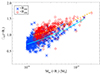 |
Fig. 1. Iron share between ICM and stellar component as a function of the total system mass. On both axes, the quantities are computed either within R500 (blue asterisks) or within R200 (red diamonds). The two lines correspond to the linear best fit of the two datasets in log-log space. |
On average, for a given system, the iron share within R200 is slightly higher than that within R500. This is a consequence of the increase in MFe,ICM between R500 and R200, while the iron mass in stars remains roughly constant at R>R500 (see next Sect. 3.2). More specifically, this follows the distribution of gas and stars in the clusters, with the gas mass increasing more significantly than the stellar mass going from R500 to R200, namely Mgas,200/Mgas,500∼1.8, while M*,200/M*,500∼1.15.
In principle, the conclusions drawn about the iron share calculated within the given radii (overdensities) are sensitive to the distributions of gas and stars, as well as to the system total mass and environment. In the ideal case of an isolated object, the iron share at different radii should converge by enlarging the region around the centre (until the whole gas and stellar contents are taken into account). Within a cosmic structure formation framework, this is difficult to be achieved because of other structures which reside in the surrounding environment. We note that our findings in Fig. 1 are consistent with expectations about the so-called “closure” radius for cluster-size systems. By definition, this radius corresponds to the distance at which the baryon fraction reaches the cosmic value, thereby enclosing all the baryons of the system. Simulation studies on cluster-size haloes show that this condition is almost fulfilled around the virial boundary or at radii corresponding to large fractions of it (despite variations in the details of different numerical modellings – see e.g. Ayromlou et al. 2023; Angelinelli et al. 2023; Rasia et al. 2025). To first approximation, we therefore expect that most stars that enriched the ICM and most of the enriched gas should be found within the cluster R200 by the present time, where the iron share is evaluated. This is especially the case for the high-mass end of our sample, whereas for smaller systems with Mtot,500∼1014 M⊙ the outer radius examined, R200, can still be insufficient to capture all the baryons.
From an observational point of view, the iron mass in stars, MFe,* is difficult to measure directly. Thus it is often estimated by means of the detected total stellar mass, M*, assuming an average solar iron abundance,  (by mass), that is:
 (2)
(2)
This means that the iron share is evaluated observationally as (Andreon 2010; Ghizzardi et al. 2021):
 (3)
(3)
In Eq. (3),  is the solar iron abundance in mass fraction, namely
  . Based on the solar reference by Asplund et al. (2009), the Fe atomic weight AFe = 55.85, and a hydrogen mass fraction of X = 0.7, this yields
  (following Ghizzardi et al. 2021; Renzini & Andreon 2014; Maoz & Graur 2017). As a general warning, we note that any uncertainty on the iron solar abundance adopted would thus directly translate into the same uncertainty on the iron share. In particular, according to Eq. (2), keeping the assumption that the stars have on average a solar iron abundance while adopting a different solar reference value would yield different stellar iron masses.
In Fig. 2 we compare the iron share of simulated clusters within R500 against observational estimates taken from the study by Renzini & Andreon (2014) and from the X-COP cluster sample by Ghizzardi et al. (2021), as a function of Mtot,500. To this scope, in addition to the values of ϒFe(<R500) evaluated directly from the total iron mass in gas and stars and already reported in Fig. 1, we also compute the iron share via the observational approach based on Eq. (3). For the assumptions made in Eq. (3) on the average stellar metallicity and solar reference abundance, we find that the observational estimate of the iron stellar mass for our simulated clusters (Eq. (2)) is slightly smaller than the true value and thus the iron share slightly increases, as clear from the figure. The differences are anyhow minor, of less than ∼10% for the majority of the systems (75% of the sample). Within R200, the median difference between true and observational-like stellar iron mass is even smaller, of the order of ∼5% (see Appendix C and Fig. C.1).
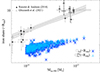 |
Fig. 2. Comparison of the iron share from simulations and observational data by Renzini & Andreon (2014) (black crosses and solid line with the grey shaded area) and Ghizzardi et al. (2021) (black open circles and dashed shaded area). The two simulation estimates of the iron share are derived by either computing directly the iron mass within stars (as in Fig. 1; large blue asterisks; “sim”) or by converting the stellar mass into iron mass assuming solar abundance, similarly to observations (Eq. (3); small cyan triangles; “obs-like”). |
The iron share predicted from simulations is significantly lower than what is obtained from cluster observations, at fixed total mass. From group to massive clusters we find a difference by a factor of 5–8 – as in Fig. 2.
The value of ϒFe in simulations confirms that gas and stars overall share a similar amount of iron, within a factor of two, despite various physical processes could impact the distributions of gas and stars in groups and clusters and their evolution in time. For instance, if the ICM within R200 comprised an accreted gas component enriched by stars that are not any longer (e.g. splash back galaxies) or not yet within the cluster volume, then the value of the iron share ϒFe(<R200) reported in Fig. 1 would be overestimated compared to the expectations of the closed-box model. Such a situation could happen when merging galaxies get stripped of their gas atmosphere, for instance after a first passage through the cluster centre, and then get shot outside R200. In terms of mass, this should be a subdominant effect, though. Instead, if part of the gas enriched by the cluster stellar component were displaced beyond the cluster virial radius and not yet re-accreted by the present time, then the ICM iron mass would be lower than the amount produced by the stars within the cluster. As a consequence, the iron share value would be also lower, compared to the closed-box model expectation. In this respect, a mass trend of the iron share can be partially connected to the impact of ejective feedback at early times (z≳2). If strong, it can push enriched gas to larger distances and the depletion of iron-rich gas content is expected to be more prominent in low-mass systems, due to their shallower potential wells, than in massive clusters, where instead a higher amount of gas can be more efficiently re-accreted by the present time (e.g. Mitchell & Schaye 2022).
Additionally, we note that part of the iron content can be comprised in a different, namely colder and denser, gas phase within the cluster, that would not contribute to the X-ray diffuse emission. The amount of this component is sensitive to the star-formation model in the simulations and to the thresholds adopted for the X-ray gas selection. In our study, we find that the total iron mass within hot and cold gas components is typically ∼10% higher (median value on the sample) than the iron mass within the X-ray gas, within both R500 and R200. The iron not included in the X-ray-emitting phase mostly resides in the core (i.e. <0.2×R500) of our simulated clusters, where it typically comprises ∼40% of the total iron gas mass and dominates the iron gas budget for ∼25% of our clusters.
3.2. Iron masses and spatial distribution
The picture of the iron share we outlined above it rooted in the spatial distribution of the iron content of the ICM and stars. Fig. 3 illustrates the median radial profile (and scatter) of the cumulative iron mass in gas and stars respectively, up to R200. From the comparison of the two median profiles, it is evident that most of the stellar MFe is enclosed within the innermost region (<0.1×R200), and roughly doubles by R200. The cumulative MFe profile for the gas is instead much steeper, increasing by ∼1.5 dex between 0.1×R200 and R200. We recall that a fraction of the iron mass is not comprised in the X-ray-emitting gas considered in Fig. 3 but rather associated to the star-forming colder gas phase. This is mostly located in the innermost region (namely <0.2×R500∼0.15R200), however, and does not impact the radial trend beyond R500. Going from R500 to R200, the increase in iron mass MFe is instead on average larger for the gas (∼55%) than for the stellar component (∼12%), similarly to the trends of total gas and stellar masses (see also Sect. 3.1). We find that the relative ratio between iron mass in the ICM and total system mass is typically almost the same within both R500 and R200. Differently, for the stellar component, this ratio decreases at R200 because the total mass increases while most of the stellar iron mass (and stellar mass) is concentrated well within R500.
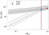 |
Fig. 3. Median radial profiles of iron mass in the ICM (solid line) and in the stellar component (dashed line) up to R200. The scatter on the sample (data comprised between the 16th and 84th percentile) is marked in both cases by the grey shaded area. The coloured symbols mark the median value of MFe in the gas (asterisks) and in the stars (stars) at R500 (blue) and R200 (red) respectively. The vertical pink line and shaded area indicate the median value of R500/R200 and the corresponding scatter. |
Despite this very different spatial distribution, the gas and stellar components share almost the same amount of iron mass within R500 or R200. In Fig. 3 this is marked by the similar median values of MFe for gas and stars at R500 and R200 (normalised to R200 in the figure – blue and red symbols, respectively), and is consistent with values of the iron share on average close to unity within both overdensities (see Fig. 1).
The total iron mass in ICM and stars within both overdensities is reported as a function of the system total mass in Fig. 4. The data points refer to the quantities computed within R500. We compute the log-log best-fit linear relations, in the form
 (4)
(4)
for gas and stars, within R500 and R200. Best-fit values for normalisation y0 and slope α are reported in Table B.1. Both gas and stellar iron masses correlate strongly with the system total mass, and the scaling shows a relatively similar normalisation, within both R500 and R200. In terms of slope, the relation between stellar MFe and total mass is always mildly shallower than the relation for the ICM iron mass.
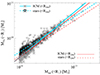 |
Fig. 4. Relation between iron mass in gas (grey asterisks) and stars (black stars) and total mass, within R500. Lines refer to the best-fit relations between MFe(<R500)–Mtot,500 (cyan lines), for gas (solid) and stars (dashed) respectively. Overplotted for comparison, the best-fit relations for the R200 region, MFe(<R200)–Mtot,200 (gas: red solid line; stars: red dashed line). |
The differences in slopes, although mild, reflect the different share of the iron content in terms of ICM and stars. This is at the origin of the trend of ϒFe with mass that can be observed in Fig. 1. In massive systems, the gas typically comprises larger amounts of iron compared to stars (ϒFe≳1), at both overdensities, with a larger difference at R200. In low-mass haloes, instead, the iron content of stars is larger than that of the gas within R500 [ϒFe(<R500)≲1], whereas it is similar within R200 [ϒFe(<R200)∼1].
3.2.1. Iron content of the ICM
In order to dissect the discrepancy between simulated and observed iron share, we compare the iron budget in the ICM to observational results. In Fig. 5 we report the relations between the ICM iron mass within R500 and both the gas mass (left) and the total mass (right) of the simulated clusters. As a comparison, we overplot the recent observational results by Ghizzardi et al. (2021) from the X-COP cluster sample, whose iron share is shown in Fig. 2. We find consistent trends in terms of slope, for both relations. For the total gas mass, Mgas,500, we consider both the cold and hot gaseous components, while for MFe,ICM(<R500) we refer to the iron mass comprised only in the X-ray emitting gas. In both cases we expect very similar results, though. Indeed, for the massive systems we select (Mtot,500>1014 M⊙), the gas budget is dominated by the hot X-ray component, which constitutes ≳95% of the total gas mass within both R500 and R200. The relation between MFe,ICM and Mgas indicates that the predictions from the simulations agree remarkably well with the observational results. Although the X-COP data mainly populate the high-mass envelope of the simulated relation, the observational best-fit relation is in very good agreement with the simulated data when extrapolated to the lower-mass regime (Mgas<5×10¹³ M⊙) as well.
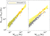 |
Fig. 5. Iron mass in the ICM as a function of gas mass (left) and total mass (right) within R500 (grey asterisks). Orange open circles with errorbars show the results for the X-COP clusters analysed by Ghizzardi et al. (2021). Best-fit observational relations from Ghizzardi et al. (2021) are also reported (solid lines) with 1-σ confidence regions (yellow shaded areas). |
In the simulated MFe,ICM–Mtot relation we note instead a systematic offset in the normalisation, compared to data. In both axes, the offset is of order of ∼50% on average. The X-COP iron gas masses are nonetheless still partially compatible with the simulation ones, at fixed total mass of the cluster, according to the uncertainties on the measurements. Considering the shift in the x-axis, we note that observational X-COP total masses refer to hydrostatic estimates, but the estimated mass bias for this specific sample is expected to be relatively small, of order of 6% at R500 (Ettori et al. 2019; Eckert et al. 2019), and cannot explain the offset between the simulated and observed trends shown in the figure. From the simulation point of view, in contrast, we should consider a 10–20% average shift towards lower masses if we were to estimate total masses through an observational-like approach under the assumption of hydrostatic equilibrium (see, e.g., Scheck et al. 2023, for mock observations with the extended ROentgen Survey with an Imaging Telescope Array, eROSITA, of a sample of clusters extracted from the same Magneticum box). The hydrostatic mass bias thus cannot explain the observed offset of Fig. 5 (right), nor it would impact the comparison with the iron share from observational data (Fig. 2) because the discrepancy is almost 1 dex. In general, we connect the shift in the normalisation of the MFe,ICM–Mtot relation to the offset in the gas-to-total mass relation between the MAGNETICUM clusters and the X-COP sample by Ghizzardi et al. (2021) (see Fig. E.3). Both simulations and observational datasets are nonetheless consistent, within the uncertainties, with the relationship proposed by Eckert et al. (2021), which aims at defining the fgas–Mtot region occupied by the majority of recent observational findings presented in the literature.
From Fig. 5, we conclude that the iron mass in the gas component of the simulated clusters is consistent with the one estimated for the X-COP clusters, at a given total gas mass. This is in line with the fact that the mass-weighted iron abundance profiles for the MAGNETICUM clusters analysed here are largely consistent with those of the X-COP sample by Ghizzardi et al. (2021) (see Appendix A).
Further ICM chemical abundances in the MAGNETICUM simulation have been previously explored by Dolag et al. (2017) across various mass ranges. They also find consistent results in comparison to a variety of observations. These different analyses all point towards an overall consistent picture of gas chemical properties in the simulated clusters investigated in this work. We thus explore the stellar-component properties in order to interpret our results on the iron share.
3.2.2. Iron content of the stellar component
For what concerns the stellar budget, we showed in Sect. 3.1 that an observational-like estimate of the iron mass in the stellar component of simulated clusters, according to Eq. (3), does not impact significantly our conclusions on the (simulated) iron share (see Fig. 2), since it only leads to a moderate (≲10%) underestimation of the true value in most cases. We thus inspect directly the stellar component in simulated clusters in order to single out the possible origin of the iron share discrepancy with respect to observational results.
In the MAGNETICUM sample we find a relatively flat, mildly decreasing, relation between the stellar mass fraction and the system total mass, for both R500 and R200. For simplicity, we only show our results for R500 in Fig. 6. On average, we find typical values of f* around 3% within R500 and closer to 2% within R200, as marked by the median values in four bins of total mass reported in the figure (cyan asterisks and shaded areas). The intrinsic scatter of the stellar fraction is small, of the order of 0.23% and 0.16%, at R500 and R200 respectively, i.e.  in both cases. This is significantly smaller than the scatter typically measured in observed stellar fractions (e.g. Andreon 2012b; Molendi et al. 2024).
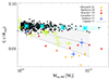 |
Fig. 6. Relation between stellar fraction and total mass within R500. Black asterisks refer to the simulated clusters in the MAGNETICUM sample, with median values and scatter in four bins of total mass marked in cyan. Observational data are taken from Laganá et al. (2011), Andreon (2012b), Gonzalez et al. (2013), Kravtsov et al. (2018), Starikova et al. (2020) and Ghizzardi et al. (2021), marked as in the upper-right legend. |
In Fig. 6, we compare the simulation results to observational measurements taken from Laganá et al. (2011), Andreon (2012b), Gonzalez et al. (2013), Kravtsov et al. (2018), Starikova et al. (2020) and Ghizzardi et al. (2021). Overall, we note a broad agreement with the reported observational findings for the low-mass systems (Mtot,500≲2–3×10¹⁴ M⊙). At the scales of massive systems (Mtot,500≳3–4×10¹⁴ M⊙), simulated stellar fractions are a factor of ∼2–3 higher than observed ones, with the majority of the data roughly converging around f*∼1–2%. Among the observational datasets reported, Ghizzardi et al. (2021) find the lowest values (f*∼0.7% on average) for the X-COP massive clusters used to estimate the iron share discussed in Sect. 3.1. In this case, there is a factor of ∼4–5 difference with respect to the stellar fractions derived from our simulated clusters. Based on the stellar iron mass estimate from Eq. (2), such difference between simulations and observations in stellar fraction would translate directly into an equal difference in the stellar iron mass (see Appendix C), and thus in the iron share.
An overall similar picture is also obtained for the measurements of the stellar component within R200 (as shown in Appendix E), given that no strong variation in the stellar-to-total mass ratio is typically observed in cluster outskirts, R500<r<R200 (Andreon 2015). Data by Andreon (2010, 2012b) suggest stellar fractions decreasing from about 4% at Mtot∼1014 M⊙ to 0.6% at Mtot∼1015 M⊙. This is in contrast with the flatter relation around 2–3% predicted by the simulations (see Fig. E.1). A recent determination by Sartoris et al. (2020) for the massive Abell S1063 cluster (Mtot∼2.9×10¹⁵ M⊙ within a radius of R200∼2.6 Mpc) at redshift z≃0.35 reported nonetheless a stellar fraction within R200 of f* = 1.5%±0.4%. This is higher than the figures typically inferred in the high-mass regime and is closer to simulation findings, as visible from Fig. E.1 in the Appendix. The value by Sartoris et al. (2020) derives from a robust, full, dynamical reconstruction of the mass profile. The authors evaluate the BCG stellar mass from spectral-energy-distribution (SED) fitting (assuming a Salpeter IMF) of high-quality VLT MUSE spectra, and further account for 1234 spectroscopically confirmed cluster members up to R200, for which stellar masses are derived from SED fitting of WFI photometric data from observations with the ESO 2.2m telescope.
We stress that results about stellar fractions from numerical simulations could be strongly impacted by the modelling of the different physical processes included (such as gas cooling and SN/AGN feedback), as well as by numerical resolution. Part of the difference can also be related to the treatment of the diffuse stellar component and its contribution to the total stellar mass. In observations, the stellar content of groups and clusters of galaxies has been extensively studied, especially at low redshift (z≲0.1, for the majority of the works reported here). By comparing the different observational datasets, a large scatter in terms of both slope and normalisation is found (e.g., see Eckert et al. 2019). In addition to the sensitivity of the inferred stellar mass on the assumed IMF, the major source of uncertainty in observations is in fact the achievement of a comprehensive census of the stellar population out to large radii, including also the tenuous ICL component and the unresolved low-mass galaxies. Whereas the ICL contribution is always included in our measurements of total stellar masses from simulations (unless otherwise stated), not all the observational studies reported account for this diffuse stellar component. For this reason, we inspect in the following the impact of measuring stellar masses within fixed apertures around the BCG instead of considering the whole stellar component within the cluster main halo.
3.2.3. Main halo contribution to the stellar mass
In Fig. 7 we show the scaling of the simulated stellar mass M*(<R500) as a function of the total cluster mass Mtot,500. We also report some of the observational datasets from Fig. 6, as in the legend. In particular, we include the two datasets by Andreon (2012b) and Ghizzardi et al. (2021), for which we discussed the iron share estimate in Sect. 3.1, and the data by Kravtsov et al. (2018). Reflecting the results on the stellar fraction, we note a systematic overprediction of the total stellar mass from simulations within R500, for haloes with Mtot,500>2×10¹⁴ M⊙.
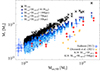 |
Fig. 7. Scaling relations between stellar mass and total halo mass Mtot,500 within R500c for the simulated clusters compared to the observational data. Simulated datapoints refer to stellar masses within R500 (M*,500; black asterisks), and to values obtained by summing up the satellite stellar mass, M*,sat, and the BCG stellar mass, M*,BCG, computed within 0.1 R500 (dark-blue asterisks), 100 kpc (blue asterisks), 70 kpc (light-blue asterisks), and 50 kpc (cyan asterisks), as in the upper-left legend. Observational data are from Ghizzardi et al. (2021) (yellow diamonds) and Andreon (2012b) (blue squares), as from their samples also the iron share estimates were derived, and from Kravtsov et al. (2018) (K18; red stars). For the latter, we report two estimates, given by the sum of the satellite stellar mass, Msat (see their Tables 1 and 4), and the BCG stellar mass within 50 kpc, MBCG(<50 kpc) (small symbols), and extrapolated to infinity from their best-fit Sérsic profile, MBCG (big symbols). |
Here, we investigate in detail the origin of this difference, by evaluating, in the simulated clusters, the specific contribution of BCGs and satellite galaxies, as identified by SUBFIND (see also Ragagnin et al. 2022). We define as satellites the substructures of the main halo that have a stellar mass M*,sat>109 M⊙ and are located within the cluster R500. The BCG is defined as the stellar component of the main halo. With this definition, we would count all the diffuse stellar halo, extending out to large radii and making up the ICL, in the BCG stellar mass. Since this component is not included in most of the observational determination of the stellar budget, we only count the stellar mass contained within the given apertures. In particular, we test different selection criteria for the BCG, computing the stellar mass within the following physical apertures: 0.1 R500, 100 kpc, 70 kpc, and 50 kpc.
For each of these four BCG definitions, the total stellar mass of the cluster region within R500 is computed as the sum of the stellar masses of the satellites2 and the BCG. This yields four different estimates of M*(<R500) (coloured, smaller asterisks in Fig. 7) in addition to the usual one computed by summing up the mass of all the stellar particles within R500 (black asterisks).
In general, we note that the decrease in the region used to estimate the BCG mass is reflected by a decrease of the resulting M* which is not constant with halo mass. The effect is stronger at higher total masses and the scaling relation effectively flattens for smaller BCG selection regions. This can be appreciated already by considering the BCG contribution within 0.1 R500. More quantitatively, we can compare the simulation results of these tests to analogous measurements available for the observational sample by Kravtsov et al. (2018) (cf. their Table 4). For instance, we report the data we obtain by summing up their values for satellites and BCG stellar masses within 50 physical kpc, M*,sat+M*,BCG(<50 kpc). In this case, the disagreement is alleviated and the difference between simulations and observational data ranges between 10% (at the low-mass end) and 40% (in massive systems), at fixed total mass. This extreme case introduces a decrease of stellar mass by a factor of ∼1.5–3, which would directly translate into the same difference in the iron stellar mass, following Eq. (2). This would let the simulated iron share value correspondingly increase by the same factor ∼1.5–3, thus getting closer to the observational estimates (see Appendix D). This further confirms that the diffuse stellar component beyond the BCG, not comprised within satellites (either small galaxies with M*<109 M⊙ or diffuse stellar component of the main halo), has a significant role in shaping the level of tension between observational findings and results from our simulated sample, in which it contributes up to 60% of the total stellar mass enclosed within R500. Carefully accounting for residual systematics in the observational inference of the stellar mass budget in clusters and for the contribution of an elusive ICM component is essential to assess the limits that the feedback processes included in simulations have in regulating star formation in such extreme environments.
3.3. Connecting star formation and the chemical enrichment of the ICM
The common underlying assumption that the stars in the cluster potential well must cause the chemical enrichment in the ICM is challenged by the high values of the iron share that are inferred from the observations of massive systems. A standard approach to investigate the amount of metal mass that could have been produced by the actual stellar population in the cluster galaxies and ejected in the cluster gas relies on semi-analytical methods. In these methods, typical prescriptions about IMF, star formation efficiency and supernova ratios are usually adopted. Studies in the literature conclude that the ICM metallicity expected from such calculations on the basis of the observed stellar mass should be lower than the metallicity actually measured from X-ray spectra (Bregman et al. 2010; Loewenstein 2013; Renzini & Andreon 2014; Blackwell et al. 2022). Here, we test semi-analytical findings by confronting the actual ICM metallicity in the simulated clusters and the predictions from stellar evolution models based on the stellar component.
In particular, we focus on the study by Loewenstein (2013) (L13) that gives a relation between ICM iron abundance and stellar-to-gas mass ratio expressed as
 (5)
(5)
where the factor β is directly proportional to the total specific number of SNe per unit stellar mass formed available to enrich the ICM, ηSN, increases with the fraction of stellar mass returned to the environment, r*, and varies with the SNIa-to-SNcc ratio, RSN (see Sect. 2.4 of L13 for more details). L13 derives the value β = 0.155 for  , r* = 0.35, RSN = 0.44, a ‘diet Salpeter’ IMF (which is a slight modification of the Salpeter IMF that assumes a flat distribution of stellar masses below 0.6 M⊙; Bell & de Jong 2001) and metal yields from Kobayashi et al. (2006).
To better relate the discrepancy in the iron share to the stellar and gas components, we bracket the validity of the L13 prediction and investigate the relation between the ICM iron abundance and the stellar-to-gas mass ratio directly in our simulated clusters. We compute ZFe both directly from the simulation outputs (“true” value) and from the L13 prediction in Eq. (5) (“L13” value). In Fig. 8 (left) the true mass-weighted ZFe/ZFe,⊙ is reported as a function of the simulated f*/fgas (black asterisks), for the region within R200. The true ICM iron abundance mildly increases with the stellar-to-gas fraction, but the relation based on the simulation outputs is overall flatter than the one predicted by L13 in Eq. (5) (solid blue line in the Figure). In general, the L13 relation predicts higher ICM enrichment levels mostly at large f*/fgas, mainly corresponding to small-mass systems (see discussion below and Appendix E). For a more quantitative comparison, we also report the best fit to the simulation data assuming two functional forms. First, we adopt a linear function similar to the L13 one, i.e. ZFe/ZFe,⊙=B×(f*/fgas), for which the best-fit value is B = 1.15 (corresponding to β = 0.115). Then, we test a second functional form:
 (6)
(6)
for which we find the best fit for A = 0.11 and B = 0.67. Thanks to the additional offset parameter A, Equation (6) provides a better fit (smaller residuals) to simulation results. These fits are valid in the range 0.15≲f*/fgas≲0.40.
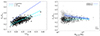 |
Fig. 8. Comparison between the simulated ICM mass-weighted iron abundance ZFe/ZFe,⊙ and the L13 prediction based on the stellar-to-gas fraction f*/fICM as in Eq. (5) for the region within R200. Left: relation between ZFe/ZFe,⊙ and f*/fICM for the simulated clusters (black asterisks), compared to the L13 relation (blue solid line). Overplotted two best-fit relations (cyan solid and dot-dashed lines, as in the legend) to the simulation data. Right: iron abundance as a function of simulated gas masses. Two estimates of ZFe/ZFe,⊙ are compared: the mass-weighted value computed directly from the simulation (“true”; black asterisks) and the value predicted for each simulated cluster given its stellar-to-gas fraction (“L13”; grey triangles). We mark median values in five mass bins for both the true (dashed cyan line) and the L13 (solid blue line) estimate, as well as the respective scatter (shaded areas) between the 16th and the 84th percentile of the distributions. |
In our simulated clusters, at each simulation timestep and for each stellar particle, ηSN, RSN and r* derive directly from our time-dependent stellar-evolution calculations (that include both metal spreading and stellar-mass loss during AGB phases and SNIa/SNcc events; see Sect. 2). We do not impose nor calibrate any relation between star formation (or metallicity) and f*/fgas. Simulated stellar mass fractions result consistently from the gas thermal cooling/heating and environmental properties. The metal distribution is additionally affected both by dilution due to mergers and by feedback mechanisms, that can halt star formation temporarily and impact the spreading of heavy elements away from star-forming regions.
Differences, albeit modest, between the L13 relation and the one found in simulations can also be introduced by different assumptions in the stellar evolution model. The choice of the IMF also plays a role during the metal budget buildup (e.g. Tornatore et al. 2007). For instance, the number of SNe per unit stellar mass is sensitive to the chosen IMF, but stellar masses decrease only by a factor of ∼1.24 when passing from a diet Salpeter IMF to a Chabrier IMF (Bell et al. 2003; Gallazzi et al. 2008; Herrmann et al. 2016). Commonly adopted values for the stellar return fraction typically range between r*≃0.26 and r*≃0.45 for different assumptions on stellar metallicity, IMF and metal yields (e.g. Fardal et al. 2007; O’Rourke et al. 2011; Vincenzo et al. 2016). Here, we have verified that the z = 0.07 median return fraction predicted from our simulated stellar populations in the clusters is r*∼0.41, in line with the expectations for a Chabrier IMF (which is adopted in our simulation runs and which is used to evaluate SN quantities at each timestep for each stellar population) and fairly close to the diet Salpeter assumption in L13. The chosen stellar yields affect only slightly the overall normalisation of ZFe and the total metallicity (e.g. Tornatore et al. 2007; Maio et al. 2010; Buck et al. 2021). Therefore, details in the stellar-evolution modelling have little impact on improving the almost 1-dex discrepancy between observations and simulations in the iron share. Overall, since L13-based gas metallicities and simulation-based gas metallicities differ by only a factor of ≲1.5 at all f★/fgas ratios and since the expected ICM iron mass is roughly consistent with observational data (as shown e.g. in previous Fig. 5), the much larger discrepancy in the iron share has to be mostly related to the different (higher) f*/fgas regime spanned by our clusters.
As a further check in our analysis, we inspect in Fig. 8 (right) the discrepancy between true iron abundance (black asterisks) and L13 prediction (grey triangles) as a function of gas mass. For both L13 expectations and simulation predictions, the scatter on the iron abundance is of about 0.02–0.04 ZFe,⊙ over the whole cluster mass range. This is essentially introduced by the scatter in the relation between f*/fgas and mass of the simulated clusters (see Appendix E). Overall, the true ICM iron abundance is fairly similar for all halos in our mass range, with a shallow mass dependence that is in agreement with most simulation results already reported in the literature from group to cluster regime (e.g. Fabjan et al. 2010; Dolag et al. 2017; Truong et al. 2019; Pearce et al. 2021; Nelson et al. 2024). Compared to the true abundances, the values predicted according to L13 are on average ∼34% higher. This difference is in fact mass dependent, with larger discrepancies for poor clusters and groups (roughly 40%) than for massive clusters (few percents). This mass trend is due to the different impact of feedback in different mass regimes. Indeed, in the shallower potential wells of small systems not all the baryons involved in the metal cycle are enclosed within R200 by the present time and part of the metal-rich gas is likely displaced out of R200. This turns into an ICM enrichment level similar to massive systems, but lower than expected (according to the L13 prediction) from their higher f*/fgas values measured within R200 (see the decreasing, albeit shallow, trend of f*/fgas(<R200) with total mass Mtot,200 in Fig. E.2). At variance with observations, the true ICM metallicity in the simulated massive clusters (Mgas,200≳5×10¹³ M⊙) is fairly consistent with the L13 expectation based on the stellar-to-gas mass fraction. In the high-mass end of our sample, true and L13-predicted ICM iron abundances differ by less than ∼10%, further stressing that the simulated ICM enrichment level is essentially consistent with predictions from semi-analytical stellar evolution models. As commented above, the small differences seem thus to be related to the different modelling techniques. Namely, changes in the amount of metals produced can be due to small variations in the assumptions underlying the L13 estimate compared to the MAGNETICUM simulations, as well as to the impact of highly non-linear processes followed by the simulations (such as star formation, feedback mechanisms and accretion/merging events) throughout the whole cluster evolution. All these phenomena impact the enrichment process and contribute in a non-trivial way to, for instance, the spreading of metal-enriched gas, the manner metals are reincorporated into newly formed stars and the spatial distribution of gas and stars within systems of different mass. The relation with the total gas mass in Fig. 8 (right) further indicates that all these effects impact more the low-mass (high-f★/fgas) regime than the massive clusters, where instead the iron-share discrepancy is the largest. This means that the much bigger offset between the observationally inferred iron share and the corresponding theoretical expectations cannot be easily reconciled with simple model variations, but is rather dependent on differences in the stellar-to-gas relative contributions to the total mass budget.
3.4. Effective iron yield
Lastly, we inspect the effective iron yield, which is another way of quantifying the efficiency with which stars produce iron in clusters. It is defined as the ratio between the total iron mass contained in cluster gas and stars (MFe,gas+MFe,*) and the initial mass of the cluster stellar component (M*,0):
 (7)
(7)
This can also be expressed in solar units as  and evaluated within a spherical region of radius RΔ. The initial stellar mass, M*,0, is typically higher than the present-day mass of the stars in the cluster (M*) due to stellar mass losses during the temporal evolution of the stellar populations, namely
 (8)
(8)
for an effective stellar mass return fraction r*. In our simulations, the initial mass of every stellar particle is stored in every snapshot output, so that we can directly compute the total M*,0 for the stars located in the clusters. This further allows us to verify the cumulative mass loss of the stars in the clusters, where multiple stellar populations of different ages co-exist and the whole cosmic evolution has occurred by the late-time snapshot considered. We find that the effective return fraction for our clusters by z = 0.07 is in fact consistent with r*∼0.41 (as expected theoretically for a Chabrier IMF, adopted in our runs). This is also fairly close to the value adopted in observations, where M*,0 has to be estimated from Eq. (8) by assuming a value for r* (e.g. M* = 0.58×M*,0, i.e. r* = 0.42, both in Renzini & Andreon 2014 and Ghizzardi et al. 2021).
Simulation results on the effective iron yield are displayed in Fig. 9 as a function of total mass, within R500. For comparison, we also report observational estimates by Renzini & Andreon (2014) and Ghizzardi et al. (2021), as in Fig. 1. Consistently with the picture sketched by the iron share, in the simulations we find a flatter relation between yFe and system mass. This translates into a difference by a factor of ∼3–5 between simulated and observed effective iron yield (depending on the observational dataset) in massive systems (Mtot,500≳4×10¹⁴ M⊙), with simulations indicating a lower efficiency in the iron production by the cluster stars.
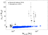 |
Fig. 9. Effective iron yield as a function of cluster mass within R500. Simulation data are marked by blue asterisks, and compared to observational data by Renzini & Andreon (2014) (black crosses) and Ghizzardi et al. (2021) (black open circles). |
From Eqs. (7) and (8), we note that the quantities involved in the effective iron yield are essentially the same at play in the iron share, so that they make a consistent description of the iron production and circulation between stars and gas. The discrepancy between simulated results and observational estimates is thus ascribed to the same factors, mostly to the different stellar mass to total mass relation (on which both stellar iron mass and initial stellar mass depend) and, to a minor extent, to some difference in the gas-to-total mass relation (see Sects. 3.2.1 and 3.2.2, and the following discussion in Sect. 4). In particular, these differences consist in the overprediction of both the total iron mass in massive clusters (MFe,gas+MFe,*) and the initial stellar mass (M*,0=M*/(1−r*)) in simulations. According to Eq. (7), the size of the discrepancy in the iron yield between simulations and observations is therefore partially alleviated compared to the iron share case.
In the following, we thus concentrate our discussion on the iron share result, which in principle is a quantity more directly measurable in observations as well, by considering only the present-day gas and stellar content.
4. Discussion
The excess of observed iron abundance with respect to the predictions from stellar-evolution models, based on the observed stellar content, represents the main inconsistency in the picture of the cluster enrichment suggested by observations. In general, the relation between iron share and total mass is expected to be impacted by the way stellar and gas distributions vary as a function of the total cluster mass.
For the galaxy clusters extracted from a MAGNETICUM simulation box, we find a flatter relation between f* and mass, compared to observations, with simulation predictions in line with observed results only at the scale of poor clusters, while predicting too much stellar mass in the most massive systems. The flat trend of f* with mass in our sample is consistent with findings on the stellar-to-halo mass relation in the regime of clusters (Mtot>1014 M⊙) based on halo occupation distribution models (Shuntov et al. 2022). Furthermore, we find a mildly increasing trend of fgas with total mass, as shown in Fig. E.3, which makes the dependence of the stellar-to-gas fraction, f*/fgas, on total cluster mass shallow, especially within R200 (see Appendix E). These results and the shallow dependence of ZFe,gas on f*/fgas also reflect the almost flat trend of ZFe,gas with total mass found in simulated clusters (Fabjan et al. 2010; Dolag et al. 2017; Biffi et al. 2018a; Truong et al. 2019; Pearce et al. 2021; see also recent observational results by Yates et al. 2017; Mernier et al. 2018a; Gastaldello et al. 2021; Mernier & Biffi 2022). These considerations explain why the iron share of simulated clusters is only mildly increasing with the cluster total mass, and robustly predict a much flatter trend than reported by observational investigations. Differently, the precise value of the iron share strongly depends on the exact level of enrichment and on the total gas and stellar budget. In our study, the discrepancy in the value of simulated and observed iron share in massive clusters can be explained by the combination of two main factors. Each of them inevitably depends on the specific simulation and observational dataset used for the comparisons. Considering the gas budget, iron abundances and iron masses are broadly consistent between the MAGNETICUM clusters and several observational samples, at a given total gas mass. With respect to the X-COP dataset, used for comparisons of the iron share, the scaling between gas iron mass and gas total mass in simulated clusters agrees very well in terms of both normalisation and slope. The agreement is in fact found throughout the mass range explored, not only at the high-mass end where the two datasets overlap. There is an offset in the gas-to-total mass relation (see Fig. 5 and Appendix E), however, that induces an additional factor of ∼1.5 difference in the gas iron mass, and thus in the iron share, at fixed total cluster mass. Based on this difference, the bias likely affecting the observational hydrostatic mass estimates would not be sufficient to reconcile the results. In particular, an average mass bias of 10–20% applied to the MAGNETICUM masses to mimick the observational measurements would not significantly ameliorate the results on the iron share nor on MFe,ICM−Mtot relation, and we can thus safely ignore it. The dominant contribution to the iron share discrepancy between simulations and X-COP data is due to the difference by a factor of ∼5 in stellar mass, and hence in the resulting stellar iron mass, at fixed halo mass. Ghizzardi et al. (2021) draw a somewhat similar conclusion based on the systematics affecting their observational measures. Namely, they argue that the uncertainties affecting the ICM iron mass estimate are the smallest ones, while systematics on the stellar component are dominant and impact the resulting iron share the most.
In light of these results, reducing the discrepancy between simulations and observations in the stellar-to-total mass relation would largely alleviate the mismatch on the iron budget. While differences in the normalisation can always be due to uncertainties in the underlying assumptions of the stellar evolution model, a flatter f*–Mtot relation, as expected from theoretical studies, would definitely help reconciling observations with the predicted iron yield in the cluster regime (and iron share; Renzini & Andreon 2014; Molendi et al. 2024). From the simulation point of view, further work on the star formation modelling is also required. Currently, most simulation results tend to overpredict the stellar masses in cluster-size haloes, producing too massive BCGs and overly massive main halos (namely the sum of the BCG and the diffuse stellar component), compared to observations (see e.g. recent results by Teklu et al. 2017; Bahé et al. 2017; Pillepich et al. 2018; Henden et al. 2020; Bassini et al. 2020; Ragagnin et al. 2022; Nelson et al. 2024). Compared to observations, the stellar mass function for the MAGNETICUM simulations at redshift z = 0 predicts too many galaxies both at the low-mass end and at the highest masses, whereas a good agreement is found in the intermediate regime (at masses ∼1010–1011 M⊙; Dolag et al. 2025). Also the star formation history in BCGs from simulations adopting similar physical modelling as the MAGNETICUM ones is still partially in contrast with observational findings, suggesting a residual star formation activity at late times which is not detected in observations of low-z BCGs (Ragone-Figueroa et al. 2018). On the other hand, a suppression of star formation in simulations should be achieved by maintaining an efficient production and circulation of metals, in such a way as to preserve the agreement between the observed and the simulated ICM enrichment level.
An additional source of discrepancy between simulated and observational measurements of stellar masses can be the comparison method itself (Munshi et al. 2013; Brough et al. 2024). In fact, in both cases, a conversion between stellar light and mass must be adopted, requiring unavoidable assumptions on the cluster stellar population properties, the IMF, the star formation history (Behroozi et al. 2010). From the purely observational point of view, a large variance in the measurement of stellar masses from various datasets is intrinsically present, as visible from Fig. 6. Especially in massive systems, uncertainties on galaxy stellar masses and difficulties in detecting and estimating the fainter diffuse stellar component likely lead to an underestimation of the observed masses, and consequently of the iron budget in stars. The definition of ICL in observations is ambiguous per se and different methods provide different results compared to estimates from simulations, where the identification of the diffuse stellar component is also non-trivial (Dolag et al. 2010). Remus et al. (2017) showed that the diffuse stellar component around massive galaxies within group and cluster environments in the MAGNETICUM simulations reproduces the spatial distribution of the observed ICL as well as its kinematic properties. Testing the observational approaches on mock images of simulated clusters extracted from different simulations, including MAGNETICUM, Brough et al. (2024) recently showed that on average all simulations provide consistent results, with BCG+ICL fractions of 0.38±0.16. Compared to the simulation values, they find all observational measures to be biased towards underestimating the ICL fractions (yielding BCG + ICL fractions of 0.13±0.05 on average). The authors also point out that among different methods and different simulations the range of BCG + ICL fractions obtained is actually substantially large, with several aspects such as projection effects contributing to enhance the uncertainties. Nonetheless, Brough et al. (2024) conclude that the discrepancy between observations and simulations mainly resides in observers and simulators often measuring different quantities, while inherent differences related to the specific simulation model are subdominant in this respect.
The underestimation of the observed stellar mass in massive haloes is indicated as part of the origin of the iron conundrum also by recent studies. Ghizzardi et al. (2021) discuss various possible uncertainties affecting the calculation of iron yield and iron share, concluding the most prominent ones are associated to the contribution of the ICL to the total cluster luminosity (up to ∼50%) and to the systematic errors in the stellar mass estimates (up to ∼60%). Molendi et al. (2024) propose an observation-based model for the chemical enrichment of clusters which implies a flat relation between the iron yield and the halo mass. Despite favouring a flat relation between stellar fraction and total mass, the main difference between the model proposed by Molendi et al. (2024) and the simulation-based picture outlined here lies in a lower normalisation for massive systems, implying an underestimation of the stellar masses in observational analyses by ∼30%, much lower than would be required to have consistency between observational results and predictions from our simulated clusters.
5. Summary and conclusions
We have directly investigated a long-standing problem in the metal budget share between the ICM and stars in massive galaxy clusters by analysing a large set of 448 simulated systems with masses Mtot,500>1014 M⊙ extracted from the MAGNETICUM simulation set at z = 0.07. The cosmological hydrodynamical simulations included a sub-resolution treatment of a wide variety of physical processes (see Sect. 2), including a detailed chemical evolution model following a metallicity-dependent cooling, a sub-resolution model of star formation from a multi-phase ISM, and the production and release of chemical elements from stars into the surrounding gas (Tornatore et al. 2004, 2007). This allowed us to test whether the stars that are included in the simulated clusters at the present epoch suffice to explain the ICM enrichment. The answer is positive. On the one hand, this may sound like an obvious outcome of the modelling within simulations. These results further ensure, however, that the assembly process and evolution of galaxy clusters, including merging events, stellar and AGN energy feedback, accretion of pristine gas along with pre-enriched gas, and the accretion of galaxies or galaxy groups, do not significantly alter the final baryonic and metal budget in massive clusters compared to expectations from a closed-box model. When the iron share is evaluated within a sufficiently large region that is comparable to the virial region, its value is close to unity. This simulation prediction is in contrast with observational findings that indicate a much larger iron share and thus an iron conundrum: The amount of iron that is detected in the ICM through X-ray observations significantly exceeds the amount that cluster stars could reasonably have produced based on their total amount as inferred from optical and near-IR luminosities.
In the following, we briefly summarise our main results.
-
The iron share ϒFe in simulated clusters is a shallow function of the total mass, both within R500 and R200. The typical values always lie between 0.5 and 2 in the mass range we explored, with 1<ϒFe<2 for the most massive systems (see Fig. 1).
-
Compared to observational estimates of the iron share by Renzini & Andreon (2014) and Ghizzardi et al. (2021), the iron share from simulations within R500 is about eight times smaller for massive systems (Mtot,500>5×10¹⁴ M⊙), and the relation with the total mass is significantly flatter (see Fig. 2). A calculation of the iron mass in stars by assuming a constant average solar iron abundance for all stars did not improve the comparison significantly.
-
The relations between total mass and iron mass in the ICM and in stars are quite similar, only the slopes are slightly different (Fig. 4 and Appendix B). At a fixed total mass, stars comprise more iron mass than ICM in the poor-cluster regime, whereas the opposite is true for massive clusters. This can be ascribed to a stronger gas depletion in smaller systems, which yields lower iron share values than unity especially within R500.
-
The iron content in the ICM and stars within simulated clusters has a different spatial distribution. The stellar iron mass is more centrally concentrated. In the ICM, the iron mass increases substantially with radius from 0.1×R200 to R200 because the gas dominates the outskirts baryonic budget. As a consequence, the increase between ϒFe(<R500) and ϒFe(<R200) is mainly driven by the increase in the ICM (gas and) iron mass.
-
The ICM chemical properties and iron mass in simulated clusters are overall consistent with observations (Sect. 3.2.1 and Appendix A). With respect to the X-COP clusters by Ghizzardi et al. (2021), the MFe,gas–Mgas relation agrees remarkably well in terms of the slope and normalisation. The agreement is also preserved at the lower masses when the best-fit relation derived from the X-COP clusters is extrapolated. The scaling between iron mass in the ICM and total cluster mass within R500 is also consistent with observations in terms of the slope, but we found a shift in the normalisation that can be connected to a higher gas fraction at a fixed total mass for the X-COP clusters compared to our simulated sample (see Appendix E). This contributes a factor of ∼1.5 to the difference between simulated and observed iron share.
-
The stellar fraction-to-total mass relation in simulations is flatter than what is indicated by observations, with a typical scatter of ∼0.2 dex at a fixed total mass. Simulated massive clusters have higher total stellar masses (fractions) at a fixed total mass than the observed systems. This difference in the stellar component is the main driver of the iron share gap between simulations and observations. It contributes a discrepancy of a factor of 2–5.
-
The prediction of the ICM metallicity based on the stellar-to-gas mass fraction as in the semi-analytical approach by Loewenstein (2013) yields values that are relatively close to the true ICM Fe abundance as measured in the simulated clusters at the highest halo masses, while larger discrepancies between the predicted and true values are found in lower-mass systems. This relates to a flatter relation between ZFe and f*/fgas in the simulated clusters. The impact of this different relation is found to be stronger than the different underlying model assumptions for stellar evolution.
-
As indicated by the comparison between the effective iron yield in simulations and observations, we found a lower efficiency with which stars produce iron in simulated clusters, with values 1≲yFe,⊙(<R500)≲2 and a shallow mass dependence for 1014<Mtot,500 [M⊙]≲2×10¹⁵.
Our results indicate the most important directions for future investigations in this framework. From the point of view of simulations, the scaling relation between the stellar mass and the halo mass definitely requires further improvements because stellar masses in the regime of massive systems are overestimated (for individual BCG and global stellar masses). This result is shared by independent sets of simulations. In terms of star formation activity, BCGs in clusters extracted from simulations adopting a similar physical modelling as the MAGNETICUM simulations also showed some residual star formation at low redshift. This contradicts observations. Observational data at higher redshifts will thus be crucial for better constraining the star formation activity in BCG across cosmic time and for improving the modelling. Any new model dedicated to improving the description of the galactic component should nonetheless preserve the solid results that are currently obtained on the ICM properties, such as the global scaling relations, the spatial distribution, and the chemical enrichment properties. On the observational side, a better understanding of the systematics that affect the measurement of stellar masses and ICL contribution in the low surface brightness limit is definitely needed to reduce the uncertainties and to better assess by how much the current star formation and feedback models that are implemented in simulations eventually need to be revised. The new era opened by Euclid and JWST observations are of paramount importance in this respect.
As a last note, a dedicated effort should still be made to properly compare simulated and observational quantities for the stellar mass determination to reduce any biases related to the comparison method itself as much as possible.
Acknowledgments
The Authors would like to thank the anonymous referee for constructive comments that helped improving the manuscript. VB is particularly grateful to Silvano Molendi, Sabrina De Grandi and Stefano Andreon, for fruitful discussions on the observational findings about the iron share conundrum. VB would like to acknowledge the precious help of Camilla Maio in spotting a typographical error in Fig. C.1 during the revision phase. VB, UM, ER acknowledge partial support from the INAF Grant 2023 “Origins of the ICM metallicity in galaxy clusters”. ER and VB acknowledge support from the Chandra Theory Program (TM4-25006X) awarded from the Chandra X-ray Center which is operated by the Smithsonian Astrophysical Observatory for and on behalf of NASA under contract NAS8-03060. UM was supported in part by grant NSF PHY-2309135 to the Kavli Institute for Theoretical Physics (KITP). KD acknowledges support by the COMPLEX project from the European Research Council (ERC) under the European Union's Horizon 2020 research and innovation program grant agreement ERC-2019-AdG 882679. This research was partially supported by the Excellence Cluster ORIGINS and by the Munich Institute for Astr-, Particle and BioPhysics (MIAPbP) which are funded by the German Research Foundation (Deutsche Forschungsgemeinschaft, DFG) under Germany's Excellence Strategy – EXC-2094 – 390783311, and by the DFG project nr. 415510302. The calculations for the hydro-dynamical simulations were carried out at the Leibniz Supercomputer Center (LRZ) under the project pr83li (MAGNETICUM). This work has been initiated under the Project HPC-EUROPA3 (INFRAIA-2016-1-730897), with the support of the EC Research Innovation Action under the H2020 Programme; in particular, the author gratefully acknowledges the computer resources and technical support provided by CINECA. SB is supported by: the Italian Research Center on High Performance Computing Big Data and Quantum Computing (ICSC), project funded by European Union – NextGenerationEU – and National Recovery and Resilience Plan (NRRP) – Mission 4 Component 2, within the activities of Spoke 3, Astrophysics and Cosmos Observations; the National Recovery and Resilience Plan (NRRP), Mission 4, Component 2, Investment 1.1, Call for tender No. 1409 published on 14.9.2022 by the Italian Ministry of University and Research (MUR), funded by the European Union – NextGenerationEU – Project Title “Space-based cosmology with Euclid: the role of High-Performance Computing” – CUP J53D23019100001 – Grant Assignment Decree No. 962 adopted on 30/06/2023 by the Italian Ministry of Ministry of University and Research (MUR); the INFN Indark Grant.
We verified that the difference between computing the satellite masses within fixed apertures and considering the total masses by SUBFIND is minor.
References
- Akritas, M. G., & Bershady, M. A. 1996, ApJ, 470, 706 [Google Scholar]
- Andreon, S. 2010, MNRAS, 407, 263 [NASA ADS] [CrossRef] [Google Scholar]
- Andreon, S. 2012a, A&A, 546, A6 [NASA ADS] [CrossRef] [EDP Sciences] [Google Scholar]
- Andreon, S. 2012b, A&A, 548, A83 [NASA ADS] [CrossRef] [EDP Sciences] [Google Scholar]
- Andreon, S. 2015, A&A, 575, A108 [NASA ADS] [CrossRef] [EDP Sciences] [Google Scholar]
- Angelinelli, M., Ettori, S., Dolag, K., Vazza, F., & Ragagnin, A. 2023, A&A, 675, A188 [NASA ADS] [CrossRef] [EDP Sciences] [Google Scholar]
- Arnaud, M., Rothenflug, R., Boulade, O., Vigroux, L., & Vangioni-Flam, E. 1992, A&A, 254, 49 [NASA ADS] [Google Scholar]
- Asplund, M., Grevesse, N., Sauval, A. J., & Scott, P. 2009, ARA&A, 47, 481 [NASA ADS] [CrossRef] [Google Scholar]
- Ayromlou, M., Nelson, D., & Pillepich, A. 2023, MNRAS, 524, 5391 [CrossRef] [Google Scholar]
- Bahar, Y. E., Bulbul, E., Ghirardini, V., et al. 2024, A&A, 691, A188 [NASA ADS] [CrossRef] [EDP Sciences] [Google Scholar]
- Bahé, Y. M., Barnes, D. J., Dalla Vecchia, C., et al. 2017, MNRAS, 470, 4186 [Google Scholar]
- Baldi, A., Ettori, S., Molendi, S., et al. 2012, A&A, 537, A142 [NASA ADS] [CrossRef] [EDP Sciences] [Google Scholar]
- Bassini, L., Rasia, E., Borgani, S., et al. 2020, A&A, 642, A37 [NASA ADS] [CrossRef] [EDP Sciences] [Google Scholar]
- Beck, A. M., Murante, G., Arth, A., et al. 2016, MNRAS, 455, 2110 [Google Scholar]
- Behroozi, P. S., Conroy, C., & Wechsler, R. H. 2010, ApJ, 717, 379 [Google Scholar]
- Bell, E. F., & de Jong, R. S. 2001, ApJ, 550, 212 [Google Scholar]
- Bell, E. F., McIntosh, D. H., Katz, N., & Weinberg, M. D. 2003, ApJS, 149, 289 [Google Scholar]
- Biffi, V., Dolag, K., & Böhringer, H. 2013, MNRAS, 428, 1395 [Google Scholar]
- Biffi, V., Planelles, S., Borgani, S., et al. 2017, MNRAS, 468, 531 [Google Scholar]
- Biffi, V., Mernier, F., & Medvedev, P. 2018a, Space Sci. Rev., 214, 123 [NASA ADS] [CrossRef] [Google Scholar]
- Biffi, V., Dolag, K., & Merloni, A. 2018b, MNRAS, 481, 2213 [Google Scholar]
- Biffi, V., Dolag, K., Reiprich, T. H., et al. 2022, A&A, 661, A17 [Google Scholar]
- Blackwell, A. E., Bregman, J. N., & Snowden, S. L. 2022, ApJ, 927, 104 [NASA ADS] [CrossRef] [Google Scholar]
- Braspenning, J., Schaye, J., Schaller, M., et al. 2024, MNRAS, 533, 2656 [NASA ADS] [CrossRef] [Google Scholar]
- Bregman, J. N., Anderson, M. E., & Dai, X. 2010, ApJ, 716, L63 [Google Scholar]
- Brough, S., Ahad, S. L., Bahé, Y. M., et al. 2024, MNRAS, 528, 771 [NASA ADS] [CrossRef] [Google Scholar]
- Buck, T., Rybizki, J., Buder, S., et al. 2021, MNRAS, 508, 3365 [NASA ADS] [CrossRef] [Google Scholar]
- Chabrier, G. 2003, PASP, 115, 763 [Google Scholar]
- David, L. P., & Nulsen, P. E. J. 2008, ApJ, 689, 837 [Google Scholar]
- de Graaff, A., Trayford, J., Franx, M., et al. 2022, MNRAS, 511, 2544 [NASA ADS] [CrossRef] [Google Scholar]
- De Grandi, S., & Molendi, S. 2001, ApJ, 551, 153 [NASA ADS] [CrossRef] [Google Scholar]
- De Grandi, S., Ettori, S., Longhetti, M., & Molendi, S. 2004, A&A, 419, 7 [NASA ADS] [CrossRef] [EDP Sciences] [Google Scholar]
- Dehnen, W., & Aly, H. 2012, MNRAS, 425, 1068 [NASA ADS] [CrossRef] [Google Scholar]
- de Oliveira, N. O. L., Jiménez-Teja, Y., & Dupke, R. 2022, MNRAS, 512, 1916 [NASA ADS] [CrossRef] [Google Scholar]
- Di Matteo, T., Springel, V., & Hernquist, L. 2005, Nature, 433, 604 [NASA ADS] [CrossRef] [Google Scholar]
- Dolag, K., & Stasyszyn, F. 2009, MNRAS, 398, 1678 [NASA ADS] [CrossRef] [Google Scholar]
- Dolag, K., Jubelgas, M., Springel, V., Borgani, S., & Rasia, E. 2004, ApJ, 606, L97 [NASA ADS] [CrossRef] [Google Scholar]
- Dolag, K., Vazza, F., Brunetti, G., & Tormen, G. 2005, MNRAS, 364, 753 [NASA ADS] [CrossRef] [Google Scholar]
- Dolag, K., Borgani, S., Murante, G., & Springel, V. 2009, MNRAS, 399, 497 [Google Scholar]
- Dolag, K., Murante, G., & Borgani, S. 2010, MNRAS, 405, 1544 [NASA ADS] [Google Scholar]
- Dolag, K., Mevius, E., & Remus, R. -S. 2017, Galaxies, 5, 35 [NASA ADS] [CrossRef] [Google Scholar]
- Dolag, K., Remus, R. -S., Valenzuela, L. M., et al. 2025, A&A, submitted [arXiv:2504.01061] [Google Scholar]
- Eckert, D., Ettori, S., Pointecouteau, E., et al. 2017, Astron. Nachr., 338, 293 [Google Scholar]
- Eckert, D., Ghirardini, V., Ettori, S., et al. 2019, A&A, 621, A40 [NASA ADS] [CrossRef] [EDP Sciences] [Google Scholar]
- Eckert, D., Gaspari, M., Gastaldello, F., Le Brun, A. M. C., & O’Sullivan, E. 2021, Universe, 7, 142 [NASA ADS] [CrossRef] [Google Scholar]
- Ettori, S., Baldi, A., Balestra, I., et al. 2015, A&A, 578, A46 [NASA ADS] [CrossRef] [EDP Sciences] [Google Scholar]
- Ettori, S., Ghirardini, V., Eckert, D., et al. 2019, A&A, 621, A39 [NASA ADS] [CrossRef] [EDP Sciences] [Google Scholar]
- Ezer, C., Bulbul, E., Nihal Ercan, E., et al. 2017, ApJ, 836, 110 [NASA ADS] [CrossRef] [Google Scholar]
- Fabjan, D., Borgani, S., Tornatore, L., et al. 2010, MNRAS, 401, 1670 [Google Scholar]
- Fardal, M. A., Katz, N., Weinberg, D. H., & Davé, R. 2007, MNRAS, 379, 985 [Google Scholar]
- Flores, A. M., Mantz, A. B., Allen, S. W., et al. 2021, MNRAS, 507, 5195 [NASA ADS] [CrossRef] [Google Scholar]
- Fujita, Y., Tawa, N., Hayashida, K., et al. 2008, PASJ, 60, S343 [Google Scholar]
- Gallazzi, A., Brinchmann, J., Charlot, S., & White, S. D. M. 2008, MNRAS, 383, 1439 [Google Scholar]
- Gaspari, M., Melioli, C., Brighenti, F., & D’Ercole, A. 2011, MNRAS, 411, 349 [Google Scholar]
- Gastaldello, F., Simionescu, A., Mernier, F., et al. 2021, Universe, 7, 208 [NASA ADS] [CrossRef] [Google Scholar]
- Ghizzardi, S., De Grandi, S., & Molendi, S. 2014, A&A, 570, A117 [NASA ADS] [CrossRef] [EDP Sciences] [Google Scholar]
- Ghizzardi, S., Molendi, S., van der Burg, R., et al. 2021, A&A, 646, A92 [NASA ADS] [CrossRef] [EDP Sciences] [Google Scholar]
- Gonzalez, A. H., Zaritsky, D., & Zabludoff, A. I. 2007, ApJ, 666, 147 [Google Scholar]
- Gonzalez, A. H., Sivanandam, S., Zabludoff, A. I., & Zaritsky, D. 2013, ApJ, 778, 14 [Google Scholar]
- Greggio, L. 2005, A&A, 441, 1055 [NASA ADS] [CrossRef] [EDP Sciences] [Google Scholar]
- Gunn, J. E., Gott, J., & Richard, I. 1972, ApJ, 176, 1 [Google Scholar]
- Gupta, N., Saro, A., Mohr, J. J., Dolag, K., & Liu, J. 2017, MNRAS, 469, 3069 [Google Scholar]
- Haardt, F., & Madau, P. 2001, in Clusters of Galaxies and the High Redshift Universe Observed in X-rays, eds. D. M. Neumann, & J. T. V. Tran, 64 [Google Scholar]
- Henden, N. A., Puchwein, E., & Sijacki, D. 2020, MNRAS, 498, 2114 [Google Scholar]
- Herrmann, K. A., Hunter, D. A., Zhang, H. -X., & Elmegreen, B. G. 2016, AJ, 152, 177 [NASA ADS] [CrossRef] [Google Scholar]
- Hirschmann, M., Dolag, K., Saro, A., et al. 2014, MNRAS, 442, 2304 [Google Scholar]
- Hough, R. T., Shao, Z., Cui, W., et al. 2024, MNRAS, 532, 476 [Google Scholar]
- Isobe, T., Feigelson, E. D., Akritas, M. G., & Babu, G. J. 1990, ApJ, 364, 104 [Google Scholar]
- Kaiser, N. 1986, MNRAS, 222, 323 [Google Scholar]
- Kirkpatrick, C. C., & McNamara, B. R. 2015, MNRAS, 452, 4361 [Google Scholar]
- Kirkpatrick, C. C., McNamara, B. R., & Cavagnolo, K. W. 2011, ApJ, 731, L23 [NASA ADS] [CrossRef] [Google Scholar]
- Kluge, M., Hatch, N. A., Montes, M., et al. 2025, A&A, 697, A13 [NASA ADS] [CrossRef] [EDP Sciences] [Google Scholar]
- Kobayashi, C., Umeda, H., Nomoto, K., Tominaga, N., & Ohkubo, T. 2006, ApJ, 653, 1145 [NASA ADS] [CrossRef] [Google Scholar]
- Komatsu, E., Smith, K. M., Dunkley, J., et al. 2011, ApJS, 192, 18 [Google Scholar]
- Kravtsov, A. V., Vikhlinin, A. A., & Meshcheryakov, A. V. 2018, Astron. Lett., 44, 8 [Google Scholar]
- Kudritzki, R. -P., Teklu, A. F., Schulze, F., et al. 2021, ApJ, 910, 87 [NASA ADS] [CrossRef] [Google Scholar]
- Laganá, T. F., Zhang, Y. -Y., Reiprich, T. H., & Schneider, P. 2011, ApJ, 743, 13 [Google Scholar]
- Leccardi, A., & Molendi, S. 2008, A&A, 487, 461 [NASA ADS] [CrossRef] [EDP Sciences] [Google Scholar]
- Liu, A., Tozzi, P., Ettori, S., et al. 2020, A&A, 637, A58 [NASA ADS] [CrossRef] [EDP Sciences] [Google Scholar]
- Loewenstein, M. 2001, ApJ, 557, 573 [Google Scholar]
- Loewenstein, M. 2006, ApJ, 648, 230 [Google Scholar]
- Loewenstein, M. 2013, ApJ, 773, 52 [Google Scholar]
- Maio, U., Ciardi, B., Dolag, K., Tornatore, L., & Khochfar, S. 2010, MNRAS, 407, 1003 [CrossRef] [Google Scholar]
- Mantz, A. B., Allen, S. W., Morris, R. G., et al. 2017, MNRAS, 472, 2877 [NASA ADS] [CrossRef] [Google Scholar]
- Maoz, D., & Graur, O. 2017, ApJ, 848, 25 [Google Scholar]
- Marini, I., Popesso, P., Lamer, G., et al. 2024, A&A, 689, A7 [NASA ADS] [CrossRef] [EDP Sciences] [Google Scholar]
- Matsushita, K., Sakuma, E., Sasaki, T., Sato, K., & Simionescu, A. 2013, ApJ, 764, 147 [Google Scholar]
- Matteucci, F., & Recchi, S. 2001, ApJ, 558, 351 [NASA ADS] [CrossRef] [Google Scholar]
- McCarthy, I. G., Schaye, J., Bower, R. G., et al. 2011, MNRAS, 412, 1965 [Google Scholar]
- McDonald, M., Bulbul, E., de Haan, T., et al. 2016, ApJ, 826, 124 [Google Scholar]
- Mernier, F., & Biffi, V. 2022, in Handbook of X-ray and Gamma-ray Astrophysics, eds. C. Bambi, & A. Santangelo (Springer Living Reference Work), 12 [Google Scholar]
- Mernier, F., de Plaa, J., Kaastra, J. S., et al. 2017, A&A, 603, A80 [NASA ADS] [CrossRef] [EDP Sciences] [Google Scholar]
- Mernier, F., Biffi, V., Yamaguchi, H., et al. 2018a, Space Sci. Rev., 214, 129 [Google Scholar]
- Mernier, F., Werner, N., de Plaa, J., et al. 2018b, MNRAS, 480, L95 [Google Scholar]
- Mernier, F., de Plaa, J., Werner, N., et al. 2018c, MNRAS, 478, L116 [NASA ADS] [CrossRef] [Google Scholar]
- Mihos, J. C. 2019, ArXiv e-prints [arXiv:1909.09456] [Google Scholar]
- Mitchell, P. D., & Schaye, J. 2022, MNRAS, 511, 2948 [Google Scholar]
- Mitchell, P. D., Lacey, C. G., Baugh, C. M., & Cole, S. 2013, MNRAS, 435, 87 [NASA ADS] [CrossRef] [Google Scholar]
- Molendi, S., Eckert, D., De Grandi, S., et al. 2016, A&A, 586, A32 [NASA ADS] [CrossRef] [EDP Sciences] [Google Scholar]
- Molendi, S., Ghizzardi, S., De Grandi, S., et al. 2024, A&A, 685, A88 [NASA ADS] [CrossRef] [EDP Sciences] [Google Scholar]
- Montes, M., & Trujillo, I. 2018, MNRAS, 474, 917 [Google Scholar]
- Morsony, B. J., Heath, C., & Workman, J. C. 2014, MNRAS, 441, 2134 [Google Scholar]
- Munshi, F., Governato, F., Brooks, A. M., et al. 2013, ApJ, 766, 56 [NASA ADS] [CrossRef] [Google Scholar]
- Nelson, D., Pillepich, A., Ayromlou, M., et al. 2024, A&A, 686, A157 [NASA ADS] [CrossRef] [EDP Sciences] [Google Scholar]
- O’Rourke, D. J. P., Shabala, S. S., & Alexander, P. 2011, MNRAS, 418, 2145 [Google Scholar]
- O’Sullivan, E., Giacintucci, S., David, L. P., Vrtilek, J. M., & Raychaudhury, S. 2011, MNRAS, 411, 1833 [CrossRef] [Google Scholar]
- Padawer-Blatt, A., Shao, Z., Hough, R. T., et al. 2025, Universe, 11, 47 [Google Scholar]
- Padovani, P., & Matteucci, F. 1993, ApJ, 416, 26 [Google Scholar]
- Pearce, F. A., Kay, S. T., Barnes, D. J., Bahé, Y. M., & Bower, R. G. 2021, MNRAS, 507, 1606 [NASA ADS] [CrossRef] [Google Scholar]
- Peebles, P. J. E. 1980, The Large-scale Structure of the Universe (Princeton University Press) [Google Scholar]
- Pillepich, A., Nelson, D., Hernquist, L., et al. 2018, MNRAS, 475, 648 [Google Scholar]
- Price, S. H., Kriek, M., Feldmann, R., et al. 2017, ApJ, 844, L6 [NASA ADS] [CrossRef] [Google Scholar]
- Ragagnin, A., Dolag, K., Moscardini, L., Biviano, A., & D’Onofrio, M. 2019, MNRAS, 486, 4001 [Google Scholar]
- Ragagnin, A., Meneghetti, M., Bassini, L., et al. 2022, A&A, 665, A16 [NASA ADS] [CrossRef] [EDP Sciences] [Google Scholar]
- Ragone-Figueroa, C., Granato, G. L., Ferraro, M. E., et al. 2018, MNRAS, 479, 1125 [NASA ADS] [Google Scholar]
- Rasia, E., Tripodi, R., Borgani, S., et al. 2025, A&A, submitted [arXiv:2505.21624] [Google Scholar]
- Rebusco, P., Churazov, E., Böhringer, H., & Forman, W. 2005, MNRAS, 359, 1041 [NASA ADS] [CrossRef] [Google Scholar]
- Remus, R. -S., Dolag, K., & Hoffmann, T. L. 2017, Galaxies, 5, 49 [NASA ADS] [CrossRef] [Google Scholar]
- Renzini, A. 2004, in Clusters of Galaxies: Probes of Cosmological Structure and Galaxy Evolution, eds. J. S. Mulchaey, A. Dressler, & A. Oemler, 260 [Google Scholar]
- Renzini, A., & Andreon, S. 2014, MNRAS, 444, 3581 [Google Scholar]
- Renzini, A., Ciotti, L., D’Ercole, A., & Pellegrini, S. 1993, ApJ, 419, 52 [Google Scholar]
- Rihtaršič, G., Biffi, V., Fabjan, D., & Dolag, K. 2024, A&A, 683, A57 [NASA ADS] [CrossRef] [EDP Sciences] [Google Scholar]
- Sarkar, A., Su, Y., Truong, N., et al. 2022, MNRAS, 516, 3068 [NASA ADS] [CrossRef] [Google Scholar]
- Sartoris, B., Biviano, A., Rosati, P., et al. 2020, A&A, 637, A34 [NASA ADS] [CrossRef] [EDP Sciences] [Google Scholar]
- Scheck, D., Sanders, J. S., Biffi, V., et al. 2023, A&A, 670, A33 [NASA ADS] [CrossRef] [EDP Sciences] [Google Scholar]
- Schulze, F., Remus, R. -S., Dolag, K., et al. 2018, MNRAS, 480, 4636 [Google Scholar]
- Shuntov, M., McCracken, H. J., Gavazzi, R., et al. 2022, A&A, 664, A61 [NASA ADS] [CrossRef] [EDP Sciences] [Google Scholar]
- Simionescu, A., Allen, S. W., Mantz, A., et al. 2011, Science, 331, 1576 [Google Scholar]
- Simionescu, A., Werner, N., Urban, O., et al. 2015, ApJ, 811, L25 [NASA ADS] [CrossRef] [Google Scholar]
- Springel, V. 2005, MNRAS, 364, 1105 [Google Scholar]
- Springel, V., & Hernquist, L. 2003, MNRAS, 339, 289 [Google Scholar]
- Springel, V., White, S. D. M., Tormen, G., & Kauffmann, G. 2001, MNRAS, 328, 726 [Google Scholar]
- Springel, V., Di Matteo, T., & Hernquist, L. 2005, MNRAS, 361, 776 [Google Scholar]
- Starikova, S., Vikhlinin, A., Kravtsov, A., et al. 2020, ApJ, 892, 34 [Google Scholar]
- Teklu, A. F., Remus, R. -S., Dolag, K., & Burkert, A. 2017, MNRAS, 472, 4769 [NASA ADS] [CrossRef] [Google Scholar]
- Thielemann, F. -K., Argast, D., Brachwitz, F., et al. 2003, in From Twilight to Highlight: The Physics of Supernovae, eds. W. Hillebrandt, & B. Leibundgut, 331 [Google Scholar]
- Tornatore, L., Borgani, S., Matteucci, F., Recchi, S., & Tozzi, P. 2004, MNRAS, 349, L19 [Google Scholar]
- Tornatore, L., Borgani, S., Dolag, K., & Matteucci, F. 2007, MNRAS, 382, 1050 [Google Scholar]
- Tornatore, L., Borgani, S., Viel, M., & Springel, V. 2010, MNRAS, 402, 1911 [NASA ADS] [CrossRef] [Google Scholar]
- Truong, N., Rasia, E., Biffi, V., et al. 2019, MNRAS, 484, 2896 [Google Scholar]
- Urban, O., Werner, N., Simionescu, A., Allen, S. W., & Böhringer, H. 2011, MNRAS, 414, 2101 [NASA ADS] [CrossRef] [Google Scholar]
- Urban, O., Werner, N., Allen, S. W., Simionescu, A., & Mantz, A. 2017, MNRAS, 470, 4583 [Google Scholar]
- van den Hoek, L. B., & Groenewegen, M. A. T. 1997, A&AS, 123, 305 [NASA ADS] [CrossRef] [EDP Sciences] [Google Scholar]
- van der Burg, R. F. J., Hoekstra, H., Muzzin, A., et al. 2015, A&A, 577, A19 [NASA ADS] [CrossRef] [EDP Sciences] [Google Scholar]
- Vigroux, L. 1977, A&A, 56, 473 [NASA ADS] [Google Scholar]
- Vincenzo, F., Matteucci, F., Belfiore, F., & Maiolino, R. 2016, MNRAS, 455, 4183 [Google Scholar]
- Vladutescu-Zopp, S., Biffi, V., & Dolag, K. 2023, A&A, 669, A34 [NASA ADS] [CrossRef] [EDP Sciences] [Google Scholar]
- Vogelsberger, M., Marinacci, F., Torrey, P., et al. 2018, MNRAS, 474, 2073 [NASA ADS] [CrossRef] [Google Scholar]
- Werner, N., Urban, O., Simionescu, A., & Allen, S. W. 2013, Nature, 502, 656 [Google Scholar]
- White, S. D. M., & Rees, M. J. 1978, MNRAS, 183, 341 [Google Scholar]
- Wiersma, R. P. C., Schaye, J., & Smith, B. D. 2009, MNRAS, 393, 99 [NASA ADS] [CrossRef] [Google Scholar]
- Woosley, S. E., & Weaver, T. A. 1995, ApJS, 101, 181 [Google Scholar]
- Yates, R. M., Thomas, P. A., & Henriques, B. M. B. 2017, MNRAS, 464, 3169 [NASA ADS] [CrossRef] [Google Scholar]
- Zibetti, S., White, S. D. M., Schneider, D. P., & Brinkmann, J. 2005, MNRAS, 358, 949 [Google Scholar]
- ZuHone, J., Bahar, Y. E., Biffi, V., et al. 2023, A&A, 675, A150 [NASA ADS] [CrossRef] [EDP Sciences] [Google Scholar]
Appendix A: Iron abundance profiles
In Fig. A.1 we show the iron abundance profiles for the MAGNETICUM sample compared to the X-COP observational sample by Ghizzardi et al. (2021) (dark-to-light red data-points), used for comparisons on the iron share. For the 448 simulated clusters, we report the individual mass-weighted, three-dimensional profiles (thin grey lines), as well as the sample median profile with scatter (dark grey, dotted line and shaded areas). Compared to the X-COP clusters, we note that on average the simulated profiles are slightly steeper and reach a lower median value in the outermost region (r≳0.8R500). In the core, we find moderately higher abundances in simulations, but we note that this is still in agreement with some of the systems in the X-COP sample. Considering the scatter on both samples, the simulated mass-weighted profiles are overall consistent with the observed ones throughout most of the radial range. This is in line with the agreement found on the relation between total iron mass in the gas and total gas mass (see Fig. 5).
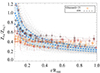 |
Fig. A.1. Iron abundance profiles up to R500 for the individual MAGNETICUM sample (thin dashed grey lines). Simulated median profile and scatter are marked as blue thick dashed line and shaded area. Coloured datapoints refer to the observational profiles for individual X-COP clusters by Ghizzardi et al. (2021), with normalisation rescaled to the reference solar abundance by Asplund et al. (2009), used for the profiles of the simulated clusters. |
Appendix B: Iron mass scaling relations
In Fig. B.1 we report the results of two different fitting methods applied to the scaling relations between iron mass, MFe, in gas (solid lines) and stars (dashed lines), and the system total mass, Mtot. As in Fig. 4, we only show the data points for the region within R500, whereas the best-fit scaling relations are reported for both R500 and R200 overdensities (in blue and red, respectively). Specifically, we compare the best-fit relations obtained in Sec. 3.2 by minimising the chi-square (grey lines) with those obtained through the BCES (Akritas & Bershady 1996) linear regression method, using the least-squares bisector method as in Isobe et al. (1990).
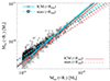 |
Fig. B.1. Same as Fig. 4, where the best-fit relations have been computed using the BCES method instead. For comparison the best-fit lines from Fig. 4 are also reported in dark (<R500) and light (<R200) grey. |
The best-fit slopes and normalisations, for both methods and overdensities are reported, with errors, in Table B.1. The two sets of best-fit relations are largely overlapping out to (6–7)×1014M⊙, with slopes consistent within the errors. Minor differences are mainly driven by the few most-massive systems (Mtot≳8×10¹⁴), and do not affect the qualitative conclusions on the main trends presented in Sec. 3.2.
Best-fit values of normalisation y0 and slope α of the MFe–Mtot relation.
Appendix C: Stellar iron content
In the simulated clusters, we verified that the iron stellar mass estimate according to Eq. 2 does not differ significantly from the direct estimate obtained by summing up the iron content of all stellar particles residing within the considered region. In particular, the observational-like estimate is on average lower than the simulation value, with a relative difference  that is ≲10% for the majority of our clusters. This difference does not depend significantly on the total cluster mass, featuring only a very weak anti-correlation quantified by a Person correlation coefficient of −0.15. This can be seen from Fig. C.1, where the two estimates of the stellar iron mass in the simulated clusters is shown as a function of Mtot,500. Based on this overall agreement between the two estimates, the stellar iron mass to total mass relation features the same scaling as the stellar to total mass relation (see Fig. 7). Compared to the observational estimates by Ghizzardi et al. (2021) for the X-COP sample (open circles) we thus find that simulated iron masses are consistently higher in simulations.
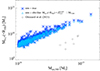 |
Fig. C.1. Stellar iron mass as a function of the total mass for the MAGNETICUM sample. We report two estimates of the iron mass in the stellar component, computed by directly summing up the iron content of all stellar particles within R500 (blue asterisks) and according to Eq. (2) (cyan triangles). For comparison, we report the X-COP observational data by Ghizzardi et al. (2021). |
Appendix D: Impact of the diffuse stellar component on the iron share
Here we show the impact on the iron share of excluding the contribution of the diffuse stellar component of the main halo beyond the BCG from the total stellar mass of the cluster, and thus from the stellar iron content. As an example, we consider the maximum correction to the stellar mass in our simulated clusters reported in Fig. 7. Namely, we consider only the stars in the clusters comprised within satellites and BCG, with the latter computed within the central 50 physical kpc (M*,sat+M*,BCG(<50 kpc), light-blue smallest asterisks in Fig. 7). The stellar iron mass, for this test, is then estimated as in Eq. (3) assuming an average solar iron abundance by Asplund et al. (2009) for all those stars. In Fig. D.1 we report the iron share of simulated and observed clusters, as in Fig. 2, with the additional dataset of simulation values for the aforementioned stellar mass definition (light-blue big triangles). The difference in cluster stellar mass directly translates in the stellar iron mass and thus on the iron share value. The latter increases by a factor of ∼2, reducing the gap with the observed values.
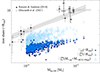 |
Fig. D.1. Same as Fig. 2, but also including the additional dataset (light-blue bigger triangles) that refers to a stellar iron mass that includes only stars within the satellites and the BCG, with the latter defined within the central 50 kpc (smallest, light-blue asterisks in Fig. 7 of the main paper). |
Appendix E: Stellar and gas fraction
In Fig. E.1 we report the relation between stellar fraction and total mass for the region enclosed within R200. Simulation data for the MAGNETICUM sample are compared against observational measurements by Andreon (2010) and Sartoris et al. (2020). Simulation results show a picture that is in line with findings at R500 (cf. Fig. 6), indicating a flatter relation compared to observations, and higher values of the stellar fraction, at fixed total mass, in the regime of massive systems. We note, however, that the observational measurement by Sartoris et al. (2020) indicates a larger stellar-to-total mass fraction (∼15%, for a system with Mtot,200∼2.9×10¹⁵M⊙), definitely closer to the simulation values.
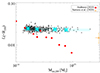 |
Fig. E.1. Relation between stellar fraction and total mass, for the region within R200. Simulation data for the MAGNETICUM sample are marked as black asterisks, with cyan big asterisks and shaded area indicating the median values and scatter in four bins of total mass. Observational data are taken from Andreon (2010) (red filled circles) and Sartoris et al. (2020) (orange triangle). |
In Fig. E.2 we report the stellar-to-gas mass fractions within R500 and R200 as a function to the system total mass Mtot,200, for the sample of MAGNETICUM clusters. We note that there is an intrinsic scatter in both relations, which is strongly reduced when the f*/fgas ratio is also computed within the larger region corresponding to R200, however. The latter is in fact expected to enclose most of the system baryons, especially in massive systems, while a larger halo-to-halo variation persists at lower masses. In smaller objects, in fact, baryonic physical processes have a stronger impact in shaping the stellar and gaseous distributions. Overall, we note that simulation values for f*/fgas are typically larger than observed values (cf., for instance, Blackwell et al. 2022). This tension is mostly driven by the larger stellar fractions predicted by simulations in massive clusters.
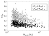 |
Fig. E.2. Stellar-to-gas fraction within the two considered overdensities (Δ = 500 and Δ = 200), both as a function of the total mass within R200. |
We report in Fig. E.3 gas masses (upper panel) and fractions (lower panel) as a function of total mass within R500, for the simulated MAGNETICUM clusters in comparison to the X-COP sample by Ghizzardi et al. (2021). In order to mark the scatter in observational measurements, we also report the best-fit functional form proposed by Eckert et al. (2021) (see their Eq. 11). As illustrated in Sec. 3.2.1, we note that the gas content in the X-COP sample is typically higher than in our simulated clusters, at fixed total mass.
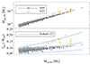 |
Fig. E.3. Upper panel: Relation between gas mass and total mass. Lower panel: Gas fraction as a function of total mass. The MAGNETICUM data are reported as grey asterisks, with median values in four bins of Mtot,500 marked by the dashed black line. Observational data points by Ghizzardi et al. (2021) (orange diamonds) and functional form derived from state-of-the-art available observations by Eckert et al. (2021) (blue line and shaded area). |
All Tables
All Figures
|
Fig. 1. Iron share between ICM and stellar component as a function of the total system mass. On both axes, the quantities are computed either within R500 (blue asterisks) or within R200 (red diamonds). The two lines correspond to the linear best fit of the two datasets in log-log space. |
| In the text | |
|
Fig. 2. Comparison of the iron share from simulations and observational data by Renzini & Andreon (2014) (black crosses and solid line with the grey shaded area) and Ghizzardi et al. (2021) (black open circles and dashed shaded area). The two simulation estimates of the iron share are derived by either computing directly the iron mass within stars (as in Fig. 1; large blue asterisks; “sim”) or by converting the stellar mass into iron mass assuming solar abundance, similarly to observations (Eq. (3); small cyan triangles; “obs-like”). |
| In the text | |
|
Fig. 3. Median radial profiles of iron mass in the ICM (solid line) and in the stellar component (dashed line) up to R200. The scatter on the sample (data comprised between the 16th and 84th percentile) is marked in both cases by the grey shaded area. The coloured symbols mark the median value of MFe in the gas (asterisks) and in the stars (stars) at R500 (blue) and R200 (red) respectively. The vertical pink line and shaded area indicate the median value of R500/R200 and the corresponding scatter. |
| In the text | |
|
Fig. 4. Relation between iron mass in gas (grey asterisks) and stars (black stars) and total mass, within R500. Lines refer to the best-fit relations between MFe(<R500)–Mtot,500 (cyan lines), for gas (solid) and stars (dashed) respectively. Overplotted for comparison, the best-fit relations for the R200 region, MFe(<R200)–Mtot,200 (gas: red solid line; stars: red dashed line). |
| In the text | |
|
Fig. 5. Iron mass in the ICM as a function of gas mass (left) and total mass (right) within R500 (grey asterisks). Orange open circles with errorbars show the results for the X-COP clusters analysed by Ghizzardi et al. (2021). Best-fit observational relations from Ghizzardi et al. (2021) are also reported (solid lines) with 1-σ confidence regions (yellow shaded areas). |
| In the text | |
|
Fig. 6. Relation between stellar fraction and total mass within R500. Black asterisks refer to the simulated clusters in the MAGNETICUM sample, with median values and scatter in four bins of total mass marked in cyan. Observational data are taken from Laganá et al. (2011), Andreon (2012b), Gonzalez et al. (2013), Kravtsov et al. (2018), Starikova et al. (2020) and Ghizzardi et al. (2021), marked as in the upper-right legend. |
| In the text | |
|
Fig. 7. Scaling relations between stellar mass and total halo mass Mtot,500 within R500c for the simulated clusters compared to the observational data. Simulated datapoints refer to stellar masses within R500 (M*,500; black asterisks), and to values obtained by summing up the satellite stellar mass, M*,sat, and the BCG stellar mass, M*,BCG, computed within 0.1 R500 (dark-blue asterisks), 100 kpc (blue asterisks), 70 kpc (light-blue asterisks), and 50 kpc (cyan asterisks), as in the upper-left legend. Observational data are from Ghizzardi et al. (2021) (yellow diamonds) and Andreon (2012b) (blue squares), as from their samples also the iron share estimates were derived, and from Kravtsov et al. (2018) (K18; red stars). For the latter, we report two estimates, given by the sum of the satellite stellar mass, Msat (see their Tables 1 and 4), and the BCG stellar mass within 50 kpc, MBCG(<50 kpc) (small symbols), and extrapolated to infinity from their best-fit Sérsic profile, MBCG (big symbols). |
| In the text | |
|
Fig. 8. Comparison between the simulated ICM mass-weighted iron abundance ZFe/ZFe,⊙ and the L13 prediction based on the stellar-to-gas fraction f*/fICM as in Eq. (5) for the region within R200. Left: relation between ZFe/ZFe,⊙ and f*/fICM for the simulated clusters (black asterisks), compared to the L13 relation (blue solid line). Overplotted two best-fit relations (cyan solid and dot-dashed lines, as in the legend) to the simulation data. Right: iron abundance as a function of simulated gas masses. Two estimates of ZFe/ZFe,⊙ are compared: the mass-weighted value computed directly from the simulation (“true”; black asterisks) and the value predicted for each simulated cluster given its stellar-to-gas fraction (“L13”; grey triangles). We mark median values in five mass bins for both the true (dashed cyan line) and the L13 (solid blue line) estimate, as well as the respective scatter (shaded areas) between the 16th and the 84th percentile of the distributions. |
| In the text | |
|
Fig. 9. Effective iron yield as a function of cluster mass within R500. Simulation data are marked by blue asterisks, and compared to observational data by Renzini & Andreon (2014) (black crosses) and Ghizzardi et al. (2021) (black open circles). |
| In the text | |
|
Fig. A.1. Iron abundance profiles up to R500 for the individual MAGNETICUM sample (thin dashed grey lines). Simulated median profile and scatter are marked as blue thick dashed line and shaded area. Coloured datapoints refer to the observational profiles for individual X-COP clusters by Ghizzardi et al. (2021), with normalisation rescaled to the reference solar abundance by Asplund et al. (2009), used for the profiles of the simulated clusters. |
| In the text | |
|
Fig. B.1. Same as Fig. 4, where the best-fit relations have been computed using the BCES method instead. For comparison the best-fit lines from Fig. 4 are also reported in dark (<R500) and light (<R200) grey. |
| In the text | |
|
Fig. C.1. Stellar iron mass as a function of the total mass for the MAGNETICUM sample. We report two estimates of the iron mass in the stellar component, computed by directly summing up the iron content of all stellar particles within R500 (blue asterisks) and according to Eq. (2) (cyan triangles). For comparison, we report the X-COP observational data by Ghizzardi et al. (2021). |
| In the text | |
|
Fig. D.1. Same as Fig. 2, but also including the additional dataset (light-blue bigger triangles) that refers to a stellar iron mass that includes only stars within the satellites and the BCG, with the latter defined within the central 50 kpc (smallest, light-blue asterisks in Fig. 7 of the main paper). |
| In the text | |
|
Fig. E.1. Relation between stellar fraction and total mass, for the region within R200. Simulation data for the MAGNETICUM sample are marked as black asterisks, with cyan big asterisks and shaded area indicating the median values and scatter in four bins of total mass. Observational data are taken from Andreon (2010) (red filled circles) and Sartoris et al. (2020) (orange triangle). |
| In the text | |
|
Fig. E.2. Stellar-to-gas fraction within the two considered overdensities (Δ = 500 and Δ = 200), both as a function of the total mass within R200. |
| In the text | |
|
Fig. E.3. Upper panel: Relation between gas mass and total mass. Lower panel: Gas fraction as a function of total mass. The MAGNETICUM data are reported as grey asterisks, with median values in four bins of Mtot,500 marked by the dashed black line. Observational data points by Ghizzardi et al. (2021) (orange diamonds) and functional form derived from state-of-the-art available observations by Eckert et al. (2021) (blue line and shaded area). |
| In the text | |
Current usage metrics show cumulative count of Article Views (full-text article views including HTML views, PDF and ePub downloads, according to the available data) and Abstracts Views on Vision4Press platform.
Data correspond to usage on the plateform after 2015. The current usage metrics is available 48-96 hours after online publication and is updated daily on week days.
Initial download of the metrics may take a while.