| Issue |
A&A
Volume 697, May 2025
|
|
|---|---|---|
| Article Number | A64 | |
| Number of page(s) | 26 | |
| Section | Interstellar and circumstellar matter | |
| DOI | https://doi.org/10.1051/0004-6361/202553822 | |
| Published online | 12 May 2025 | |
Turbulence in protoplanetary disks: A systematic analysis of dust settling in 33 disks
1
Universitá degli Studi di Milano, Dipartimento di Fisica,
via Celoria 16,
20133
Milano,
Italy
2
Centre for Star and Planet Formation, Globe Institute, University of Copenhagen,
Øster Voldgade 5–7,
1350
Copenhagen,
Denmark
3
Astronomy Unit, School of Physics and Astronomy, Queen Mary University of London,
London
E1 4NS,
UK
4
Ludwig-Maximilians-Universität München, Universitäts-Sternwarte,
Scheinerstr. 1,
81679
München,
Germany
5
Univ. Grenoble Alpes, CNRS, IPAG,
38000
Grenoble,
France
6
Jet Propulsion Laboratory, California Institute of Technology,
4800 Oak Grove Drive,
Pasadena,
CA
91109,
USA
7
Astronomy Department, University of California Berkeley,
Berkeley,
CA
94720-3411,
USA
8
California Institute of Technology,
Pasadena,
CA
91125,
USA
9
Max-Planck Institute for Astronomy,
Königstuhl 17,
69117
Heidelberg,
Germany
★ Corresponding author: This email address is being protected from spambots. You need JavaScript enabled to view it.
Received:
20
January
2025
Accepted:
22
February
2025
Abstract
The level of dust vertical settling and radial dust concentration in protoplanetary disks is of critical importance for understanding the efficiency of planet formation. Here, we present the first uniform analysis of the vertical extent of millimeter dust for a representative sample of 33 protoplanetary disks, covering broad ranges of disk evolutionary stages and stellar masses. We used radiative transfer modeling of archival high-angular-resolution (≲0.1″) ALMA dust observations of inclined and ringed disks to estimate their vertical dust scale height, which was compared to estimated gas scale heights to characterize the level of vertical sedimentation. In all 23 systems for which constraints could be obtained, we find that the outer parts of the disks are vertically settled. Five disks allow for the characterization of the dust scale height both within and outside approximately half the dust disk radius, showing a lower limit on their dust heights at smaller radii. This implies that the ratio between vertical turbulence, αz, and the Stokes number, αz/St, decreases radially in these sources. For 21 rings in 15 disks, we also constrained the level of radial concentration of the dust, finding that about half of the rings are compatible with strong radial trapping. In most of these rings, vertical turbulence is found to be comparable to or weaker than radial turbulence, which is incompatible with the turbulence generated by the vertical shear instability at these locations. We further used our dust settling constraints to estimate the turbulence level under the assumption that the dust size is limited by fragmentation, finding typical upper limits around αfrag ≲ 10−3. In a few sources, we find that turbulence cannot be the main source of accretion. Finally, in the context of pebble accretion, we identify several disk regions that have upper limits on their dust concentration that would allow core formation to proceed efficiently, even at wide orbital distances outside of 50 au.
Key words: radiative transfer / turbulence / protoplanetary disks / stars: formation
© The Authors 2025
 Open Access article, published by EDP Sciences, under the terms of the Creative Commons Attribution License (https://creativecommons.org/licenses/by/4.0), which permits unrestricted use, distribution, and reproduction in any medium, provided the original work is properly cited.
This article is published in open access under the Subscribe to Open model. This email address is being protected from spambots. You need JavaScript enabled to view it. to support open access publication.
1 Introduction
Protoplanetary disks are the birthplaces of planets. As such, understanding disk properties is critical to determining how and where planets are forming. Two main theories can explain planet formation. On the one hand, dense and cold disks can form massive planets directly from the available dust and gas via the gravitational instability process. This is similar to the star formation mechanism and is expected to create planets at large separations from their host star (>100 au). On the other hand, the core accretion scenario requires the progressive growth of initially submicron-sized particles to form larger bodies and eventually the rocky cores of giant planets. In this scenario, an important concentration of solids is necessary to accelerate the dust growth. Indeed, the streaming instability (Youdin & Goodman 2005; Johansen & Youdin 2007), currently one of the favored mechanisms allowing the sufficiently rapid growth from pebbles to planetesimals, can develop if the dust-to-gas ratio is high, of order unity. After the planetesimal formation stage, growth of planetary cores via pebble accretion (Lambrechts & Johansen 2012) is also enhanced if the layer of pebbles is vertically thin.
The spatial distribution of dust and its enhancement with respect to the gas is determined by dust–gas interactions. As dust orbits the central star, gas drag causes it to drift radially toward a local pressure maximum. In the vertical direction, initial oscillations of dust particles around the disk midplane are dampened due to gas drag, which leads dust to fall vertically toward the disk midplane. The level of dust concentration is directly related to the ratio α/St, where St is the Stokes number that parametrizes the coupling of dust with gas, and α quantifies the turbulence level in the disk. High values of this ratio imply strong mixing of dust with gas, while low values (α/St < < 1) mean that the dust is decoupled from the gas and concentrated into geometrically thin regions. Despite their critical role in planet formation, observational constraints on the level of gas turbulence and the coupling between dust and gas remain limited.
In order to explain the accretion of the disk toward the star, protoplanetary disks are predicted to be turbulent. Various hydrodynamical or magnetohydrodynamic processes can be at the origin of the physical gas turbulence in disks (see Lesur et al. 2023, for a review) and still need to be constrained by observations. Both the strength and isotropy of the predicted turbulence can be compared with observations. For example, mechanisms such as the vertical shear instability (VSI, Nelson et al. 2013) imply very strong vertical turbulence associated with weak radial mixing (e.g., Stoll et al. 2017). On the contrary, gravitational instability results in the opposite anisotropy of turbulence (e.g., Béthune et al. 2021), while mechanisms such as the streaming instability, embedded planets, or ambipolar diffusion imply turbulence of similar strength in both the vertical and radial directions (e.g., Youdin & Goodman 2005; Simon et al. 2013). Finally, alternate views can also explain accretion without requiring turbulence, as in the case of MHD winds for example (e.g., Bai & Stone 2011; Tabone et al. 2022; Lesur et al. 2023).
Measuring the strength of turbulence is notoriously difficult (see Rosotti 2023, for a recent review), in part because turbulence is predicted to be very weak (α ≪ 1). Direct measurements via line broadening have been performed in about half a dozen systems (Flaherty et al. 2015, 2018, 2020; Teague et al. 2016), typically finding that weak turbulence, α ≲ 10−3, may be common (although there are exceptions, see e.g., Paneque-Carreño et al. 2024; Flaherty et al. 2024). These studies are, however, limited to a few objects, due to the high quality of the observations required, and only allow for the measurement of a global value for the turbulence strength at the disk surface. On the other hand, the radial and vertical concentration of dust can allow us to go beyond these limitations and evaluate the variation and anisotropy of turbulence throughout the disk and for a larger number of objects. Dust accumulation also traces the turbulence at the disk midplane, which is important for dust growth.
Thanks to ALMA, several dozen of protoplanetary disks have been observed at high angular resolution (≲0.1″). These observations have revealed a broad range of substructures in millimeter continuum, with annular rings being the most common (Andrews et al. 2018; Long et al. 2018). Such observations can be used to directly observe and characterize the radial and vertical structure of protoplanetary disks, and obtain insights into the turbulence levels and structure in the disks. High-angular-resolution observations of edge-on disks are the most direct way to retrieve information on their vertical structure (Villenave et al. 2020, 2022; Lin et al. 2021, 2023; Sturm et al. 2023). However, such systems are relatively rare (~20–30 are currently known, Angelo et al. 2023), and do not provide a good view of their radial structure. On the other hand, systems at intermediate inclinations that possess clear ring and gap features are favorable targets to constrain both the vertical (Pinte et al. 2016; Doi & Kataoka 2021; Pizzati et al. 2023) and radial (Dullemond et al. 2018; Rosotti 2023) concentration of dust particles. Here, we propose to expand the analysis of the vertical and radial concentration of dust to a larger sample and to systematically look for potential radial variations in the turbulence strength within the disks. Our goal is also to characterize the turbulence level and its potential anisotropy in a large sample of protoplanetary disks, and to discuss the implications regarding the origin of the turbulence and wide-orbit planet formation.
We present the analysis of archival ALMA continuum observations of 33 inclined and ringed protoplanetary disks. The sample selection and data reduction are discussed in Sect. 2. Then, Sect. 3 describes the methodology employed to model the disks. Sect. 4 introduces the results for the vertical concentration of dust in the disks. In Sect. 5, we determine the level of vertical and radial dust–gas coupling (α/St) in the different rings, and discuss the anisotropy of turbulence and implication regarding its possible origin. In Sect. 6, we break the degeneracy between α and St by assuming that the dust size is limited by fragmentation. We discuss the results in the context of disk accretion and potential for planet formation. We conclude with a discussion on the implications of our results for wide-orbit planet formation via pebble accretion (Sect. 7) and our final remarks (Sect. 8).
2 Observations
2.1 Sample
We selected disks with moderate to high inclination that present ring structures and for which good quality ALMA data at band 6 (~1.3 mm; Ediss et al. 2004; Kerr et al. 2014) or 7 (~0.9 mm; Mahieu et al. 2012) are available in the archive. We report observation characteristics of the sources in Appendix B.
We analyzed a total of 33 disks. Our sample includes 15 disks from the DSHARP survey (AS209, DoAr25, DoAr33, Elias20, Elias24, Elias27, GWLup, HD 142666, HD 143006, HD 163296, MYLup, SR4, Sz114, WaOph6, WSB52, Andrews et al. 2018), for most of which a measurement of the height with a similar technique was previously obtained or attempted by Pizzati et al. (2023). We also include five disks from the Taurus survey by Long et al. (2018, CI Tau, DL Tau, DS Tau, GO Tau, MWC 480) and one from the ODISEA survey (ISO-Oph 17, Cieza et al. 2021). Finally, the rest of the sample constitutes of 12 disks previously published in individual papers (AA Tau, DM Tau, GM Aur, Haro6-5B, HL Tau, J1608, J1610, LkCa 15, Oph163131, PDS70, RYTau, V1094Sco; Loomis et al. 2017; Hashimoto et al. 2021; Huang et al. 2020; Stephens et al. 2023; Facchini et al. 2020; Villenave et al. 2020, 2022; Benisty et al. 2021; Ribas et al. 2024; van Terwisga et al. 2018).
Table A.1 gathers the disk and stellar parameters considered for this study. Specifically, we compile the stellar masses and radii, which are input parameters required for the modeling presented in Sect. 3. For most disks, we estimate the stellar radius based on the published stellar luminosity following ![Mathematical equation: $\[R_{\star}=\sqrt{L_{\star} / 4 \pi \sigma T_{\text {eff }}^{4}}\]$](/articles/aa/full_html/2025/05/aa53822-25/aa53822-25-eq1.png) (however, see Sect. 3.3 for systems marked with * in R⋆ column of Table A.1). The sample covers a wide range of stellar masses, between 0.36 M⊙ and 2.04 M⊙. It also includes objects with different accretion rates spanning four orders of magnitudes, which could be at different evolutionary stages within the Class II phase (although young stellar object accretion is episodic, Evans et al. 2009).
(however, see Sect. 3.3 for systems marked with * in R⋆ column of Table A.1). The sample covers a wide range of stellar masses, between 0.36 M⊙ and 2.04 M⊙. It also includes objects with different accretion rates spanning four orders of magnitudes, which could be at different evolutionary stages within the Class II phase (although young stellar object accretion is episodic, Evans et al. 2009).
2.2 Data reduction
For each object, we gathered calibrated visibility files either from the ALMA archive or directly from the first publisher team. Data collected from first publisher teams are the DSHARP targets (Andrews et al. 2018), DM Tau (Hashimoto et al. 2021), Haro6-5B (Villenave et al. 2020), Oph163131 (Villenave et al. 2022), PDS 70 (Benisty et al. 2021), RY Tau (Ribas et al. 2024), and some Taurus disks from Long et al. (2018, DL Tau, DS Tau, GO Tau, MWC 758, see Tables B.1 and B.2). Those datasets had been previously self-calibrated. For datasets collected from the archive, we employed the automated self-calibration script developed at NRAO1, which was successful to improve the data quality of V1094 Sco and ISO-Oph 17. Then, for each disk, we generated an image using the tclean algorithm, using CASA version 5.1.1–5, consistently with the version used to generate the DSHARP images. All images were generated with the spectral model mfs and nterms=1. A multi-scale synthesis was used for all disks and the images were cleaned up to ~5σ. We used a briggs weighting, with a robust parameter between −0.5 and 0.5 as is indicated in Tables B.1 and B.2. We also report the root mean square (rms) of the final images in those tables. All the reduction parameters, the visibilities, and cleaned disk images have been uploaded on zenodo (zenodo.14054952). Finally, we generate a deprojected image based on the inclinations reported in Table A.1.
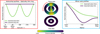 |
Fig. 1 Schematic representation of the expected effects of disk thickness. Left: effect of ring vertical thickness on the azimuthal profiles of a radially narrow, optically thin ring. A vertically thin ring (dark) shows no variation in its azimuthal profile along the ring, while a thick ring (green) displays strong azimuthal variation along the ring. Right: effect of disk vertical thickness on the minor axis brightness of a disk at the location of a gap (right). A vertically thin gapped disk (dark) shows deep gap along the minor axis, while a thick gapped disk (green) displays shallow gap along the minor axis direction. |
3 Radiative transfer modeling
In this section, we first describe the expected effect of vertical thickness to the appearance of a protoplanetary disk. Then, we detail the modeling procedure of this work, which allows us to fit each disk and obtain constraints on their vertical extent. We follow the approach that Pinte et al. (2016) developed for the case of HL Tau, and which was also used by Pizzati et al. (2023) on 15 DSHARP disks. Compared to the study of Pizzati et al. (2023), we now consistently compute the temperature structure of the disk, consider a full grain size distribution, and analyze the disk emission not only along the minor axis direction but also along several other azimuthal angles.
3.1 Expected effect of disk thickness to observed brightness
The geometrical thickness of a protoplanetary disk can have different effects on its brightness, which we summarize in this sub-section. Fig. 1 shows a schematic representation of the two main effects analyzed in this work. We consider here inclined disks or rings, with no intrinsic eccentricity and asymmetry. Gap projection effect – gaps and outer disk edges. While, after deprojection from the inclination, a gap in an infinitely thin disk will have the same shape at all azimuths, the depth and apparent width of a gap is expected to vary with azimuth in the case of a geometrically thick disk. If the disk is sufficiently inclined and vertically thick, a gap will appear less deep and less wide along the projected minor axis than along the major axis direction (see middle and right panels of Fig. 1). In other words, the depth of a gap in the projected minor axis cuts of an image can be dominated by the disk vertical thickness in inclined systems. This is the effect that has been previously analyzed for example by Pinte et al. (2016), Villenave et al. (2022), and Pizzati et al. (2023). It is most easily identifiable by using intensity cuts across the gap for different azimuthal angles. High angular resolution is critical for effectively resolving the substructures and identifying those effects. For example, a typical angular resolution of 0.1″ corresponds to 15 au at the distance of nearby star-forming regions (e.g., Taurus). At this resolution, most disk substructures remain unresolved, as is evidenced by the high fraction of smooth disks (20/32) found in the unbiased Taurus survey by Long et al. (2018). This underscores the need for higher angular resolution observations, as analyzed in this work (Appendix B).
A narrow gap configuration is the most favorable situation to identify this effect as the rings both interior and exterior to the gap can be projected on to the gap and affect its width along the minor axis direction. However, the vertical projection effect of a ring can also be visible at the outer edge of a disk. In that case, only the thickness of the disk interior to the outer (infinite) gap plays a role. In other words, the disk thickness is projected further out than the true (midplane) outer radius. A thinner disk will have a steeper outer edge profile along the minor axis direction than a thicker disk, and end at a smaller apparent radius. We refer to these effects as “G” in the case of the gap effect and “O” for the outer edge effect in Table A.2.
Ring effect. For optically thin dust, a vertically thick, radially narrow ring is expected to exhibit azimuthal brightness variations. Although it may superficially look similar, this effect is different from the well-known limb darkening in stars, which requires optically thick emission and a temperature gradient. This mechanism has been discussed in detail for disks by Doi & Kataoka (2021) and relies on the amount of material which is crossed along the line of sight and which varies at different azimuths. Along the major axis the line of sight intersects both the width, σr, and the height, σz, of the ring. Along the minor axis, however, the projected material column density is reduced due to the projection of the vertical extent of the disk, resulting in lower observed intensities, such that ![Mathematical equation: $\[I_{minor} / I_{major}= \sigma_{r} / \sqrt{\sigma_{r}^{2}+\sigma_{z}^{2} \tan ^{2} i}\]$](/articles/aa/full_html/2025/05/aa53822-25/aa53822-25-eq2.png) (Doi & Kataoka 2021). As a result, if dust is optically thin, the ring is predicted to be brighter along its major axis than along its minor axis (see left and middle panels of Fig. 1). This effect is indicated by the letter “R” in Table A.2.
(Doi & Kataoka 2021). As a result, if dust is optically thin, the ring is predicted to be brighter along its major axis than along its minor axis (see left and middle panels of Fig. 1). This effect is indicated by the letter “R” in Table A.2.
However, we note that an elongated beam might artificially create a similar azimuthal variation in a ring’s brightness in observations. To confirm that the variations are due to a vertically thick ring rather than to an imaging artifact, radiative transfer models are required and synthetic images need to be created with similar characteristics as the observations. Alternatively, creating images where the beam is circular after deprojection from the disk inclination could alleviate this problem.
Wall effect. When dust is optically thick and in the presence of a gap, the far side of the disk (wall), will be directly exposed to the observer. On the near side, the directly illuminated wall is hidden, leading to a crescent asymmetry along one side of the minor axis. The best example of disk walls are found in optically thick rings observed at scattered light wavelengths (e.g., GG Tau, Duchêne et al. 2004). At millimeter wavelengths, this effect has been clearly demonstrated by Ribas et al. (2024) in two systems, and also identified in other mid- or highly inclined disks (e.g., Ohashi et al. 2022; Lin et al. 2023; Guerra-Alvarado et al. 2024). In mid-inclination systems it only becomes relevant close to the star (≲10 au). This effect will thus not be specifically investigated in this work.
3.2 Disk structure
We assume that the disk structure is axisymmetric. For all disks, we consider an inner radius of Rin = 0.1 au and a fixed outer radius, Rout, as is indicated in Table A.1. The vertical density distribution of the gas is parameterized by a power law such that:
![Mathematical equation: $\[H_{\mathrm{g}, ~\operatorname{model}}(r)=10~(r / 100 ~\mathrm{au})^{1.1}, \text { for } R_{\mathrm{in}}<r<R_{\mathrm{out}}.\]$](/articles/aa/full_html/2025/05/aa53822-25/aa53822-25-eq3.png) (1)
(1)
The dust is composed of astronomical silicates and graphite grains (same composition as in Gräfe et al. 2013; Villenave et al. 2023). The distribution of dust sizes is fixed. Grains sizes a are between 0.005 μm and 3 mm and follow a power-law distribution such that n(a)da ∝ a−3.5da. We consider 100 grain size bins with a logarithmic distribution in a. The gas-to-dust ratio is constant within the disk and assumed to be 100.
We implement differential dust settling, using the prescription of Fromang & Nelson (2009). This prescription describes turbulence as a diffusive process, and the vertical density distribution for a grain of size a follows:
![Mathematical equation: $\[\rho_{\mathrm{d}}(r, z, a) \propto \Sigma_{\mathrm{d}}(r) \exp \left[-\mathrm{Sc} \frac{\operatorname{St}_{\mathrm{MCFOST}}(a)}{\alpha_{z, \mathrm{MCFOST}}}\left(e^{\frac{z^2}{2 H_{\mathrm{g}}^2}}-1\right)-\frac{z^2}{2 H_{\mathrm{g}}^2}\right],\]$](/articles/aa/full_html/2025/05/aa53822-25/aa53822-25-eq4.png) (2)
(2)
where Σd(r) is the dust surface density, and Hg is the gas scale height (Equation (1)). StMCFOST(a) is the Stokes number of the particles at the disk midplane (z = 0):
![Mathematical equation: $\[\operatorname{St}_{\mathrm{MCFOST}}(a)=\frac{\rho_{\mathrm{bulk}} a}{\rho_{\mathrm{g}, ~\operatorname{mid}} H_{\mathrm{g}}(r)}.\]$](/articles/aa/full_html/2025/05/aa53822-25/aa53822-25-eq5.png) (3)
(3)
The dust material density and gas density in the midplane are respectively described as ρbulk and ρg,mid. Sc is the Schmidt number, which quantifies the ratio of gas and dust diffusivities, and is fixed to 1.5 (Pinte et al. 2016; Fromang & Nelson 2009). The degree of settling is set by varying the turbulence parameter αz,MCFOST. For each disk, we consider 4 logarithmic levels of settling, with αz,MCFOST between 2 × 10⁻⁴ and 0.2. Because this value is model-dependent, we later refer to the models as “Flat”, “Thin”, “Moderate”, or “Thick”, respectively for αz,MCFOST = 2 × 10⁻⁴, 2 × 10⁻³, 2 × 10⁻², or 2 × 10⁻¹.
3.3 Fitting the dust surface brightness
We use the radiative transfer code mcfost (Pinte et al. 2006, 2009) to model the brightness of the disks. For each disk, we set global (distance, sky coordinates), disk (i, PA, Rout), and stellar (Teff, R⋆, M⋆) parameters based on observational constraints (Table A.1).
We produced radiative transfer models of the disks based on an estimate of their surface density profile. To do so, we first estimate an initial surface density profile, as is described below. Then, we follow the approach of Pinte et al. (2016) and Pizzati et al. (2023), and employed an iterative procedure to find a surface density profile, allowing us to reproduce the brightness profile along the major axis for each disk.
We assumed that vertical projection effects are absent or limited in the major axis direction and used this to estimate the surface density of the disk. We extracted the major axis profiles of the data I(r) from their deprojected images, using a wedge with an opening angle of 30°, averaged on both sides (i.e., for positive and negative radii). For HD 143006, HD 163296, and PDS70, however, we do not average both sides of the major axis profiles but instead consider only the side without the crescent.
An initial surface density profile was estimated using the following equation:
![Mathematical equation: $\[\Sigma_{\mathrm{d}}(r)=\frac{I(r)}{B_\nu[T(r)] \times \kappa_\nu},\]$](/articles/aa/full_html/2025/05/aa53822-25/aa53822-25-eq6.png) (4)
(4)
where Bν represents the Planck function at a given temperature. To compute the initial surface density profile using Equation (4), we assume a dust opacity of κν = 13.27 cm2/g, independently of the observing wavelength, and an initial disk midplane temperature of T = 20(r/100 au)−q, where q = 0.5 for r > 5 au and q = 0.1 for r < 5 au. These assumptions are only needed for the first iteration since the temperature structure and dust opacities are consistently calculated during the radiative transfer for all subsequent iterations.
Using this initial surface density, we generated a radiative transfer image with mcfost, for the same inclination and position angle as the data. Using these radiative transfer model images, we then produce synthetic images with the same uvcoverage as the data. This is done within CASA using the ft function. Then, synthetic model images are created using the tclean CASA task, with the same imaging parameters as the data. Finally, similarly to the data, we deproject the model image based on the disk inclination.
After extracting the major axis brightness profile of the deprojected model image, we produce a corrected dust surface density profile by multiplying the initial surface density profile by the ratio data over model. During that step, the total dust disk mass is also adjusted to match the absolute brightness of the major axis profile. We repeat the steps until the model brightness profile agrees with the data within 5% or after 20 iterations, whichever is first. We report the final dust mass for each source in Table A.2. The reported value (resp. uncertainty) is the averaged (resp. standard deviation) dust mass over the four models with different thicknesses.
This method converges most effectively for optically thin dust. For optically thick dust, the method becomes ambiguous as iterations can increase the dust mass without a corresponding increase in observed flux, and the models can fail to reproduce the major axis brightness. This is why, although included in the model, the iterative procedure is only applied between 5 au and Rout to avoid modeling the optically thick inner region. Moreover, for a few systems (GO Tau, GW Lup, HL Tau, Oph163131), the stellar parameters inferred by the literature do not allow the models to be bright enough to reach the observed flux in some bright dust rings. This is because with the literature stellar parameters, the dust temperature is too low for the models to reproduce the observations. To allow the models to converge, we decided to increase the disk temperature in order to have sufficiently bright dust in the outer disk. We performed this by artificially increasing the stellar radius, and thus the stellar luminosity, in the modeling (systems marked with * in column R⋆ of Table A.1). Physically, the stellar luminosities may have been under-estimated in the case of the presence of an envelope (e.g., HL Tau) or an edge-on disk (e.g., Oph163131). Alternatively, a different disk density profiles, not explored in this work, may allow for a warmer midplane for similar stellar parameters. The final models have been uploaded to a zenodo repository (zenodo.14056832).
3.4 Identifying the best model utilizing different azimuthal wedges and azimuthal profiles
Using the iterative procedure previously described (Sect. 3.3), we generated four models per disk, with different levels of dust sedimentation (parametrized by αz,MCFOST). All of them match the major axis profiles of the observations, while having different vertical dust height. To identify the effect of the dust vertical height on the global disk appearance, we compared data and model profiles along different azimuths. From the deprojected data and model maps, we obtained six wedges of 30°. They go from the minor axis to 15° from the major axis, allowing us to investigate different levels of projection effects along several directions.
To identify the best fitting model, or the models to be excluded, we first performed a visual check of the different cuts. We focused on specific regions in the disks. Specifically, we defined regions centered around the gaps or including the outer disk, to look for the expected projection effects (Sect. 3.1). These regions of interest were defined visually based on the major axis profile and will allow us to study if there is any variation in the settling efficiency within a given disk.
Following our initial visual identification of the regions of interest and subsequent identification of inappropriate models, we employed two quantitative metrics to assess the discrepancies between the models and the data. The first metric consists of a normalized χ2 parameter and the second criterion, 𝒮, quantifies the difference in shapes between the data and model curves. For the first metric, we average ![Mathematical equation: $\[\chi_{\text {azimuth }}^{2} / \chi_{\text {majorAxis }}^{2}\]$](/articles/aa/full_html/2025/05/aa53822-25/aa53822-25-eq7.png) over each azimuthal direction. This quantifies the distance of the model with the data but does not consider the difference in shape. The second metric estimates the Hausdorff distance (𝒮, Munkres 2000), which takes into account the likelihood in shape between the model and the data. This metric measures the “distance” between two sets of point by identifying the maximum distance between any point in one set and its nearest neighbor in the other set.
over each azimuthal direction. This quantifies the distance of the model with the data but does not consider the difference in shape. The second metric estimates the Hausdorff distance (𝒮, Munkres 2000), which takes into account the likelihood in shape between the model and the data. This metric measures the “distance” between two sets of point by identifying the maximum distance between any point in one set and its nearest neighbor in the other set.
By visual inspection, we identify that models with χ2 ≤ 8 and 𝒮 ≤ 1.2 are generally good models. In addition, we also consider the shape of the χ2 and 𝒮 curves as a function of αz,MCFOST to identify trends for better/worse models with thickness. The constraints reported in Table A.2 reflect the combined use of the metrics and of our visual analysis to exclude models. In some systems, the χ2 or the 𝒮 metric is not discriminating and is thus not considered. Appendix D shows the final values of χ2 and 𝒮 for each model, as well as the major axis profiles and other relevant azimuthal profiles providing constraints on the dust scale height, for all disks.
Finally, we note that for three disks discussed in Sect. 4.1, we also generated azimuthal profiles along their rings, to investigate the ring effect presented in Sect. 3.1. For the inner ring of these disks, the constraint to the vertical thickness was mainly obtained by visual inspection.
3.5 Getting the dust scale height for the best model
Once the best model was identified, we estimated its dust scale height, Hd. We consider only the grains that emit the most at the wavelength of the observations (Appendix B). Those grains are identified within mcfost, based on the dust properties assumed in the modeling, and have typical sizes around 100 μm (Table A.2). To estimate their dust scale height, we fit the mcfost vertical distribution of these grains, at each radius, with a 1D Gaussian. This provides us with a radial profile of the relevant dust scale height. Then, we obtained the average dust scale height in each radial region of interest, which we divide by the average radius of the region to obtain the aspect ratio Hd/R.
For completeness, we also report the corresponding αz,MCFOST of the constraining model and the Stokes number of these particles assumed in the modeling, StMCFOST, in Table A.5. However, we emphasize that the dust vertical thickness is the only quantity that can be directly constrained by the observations. If different assumptions for the Stokes number were considered in the modeling (for example because of a different dust surface density or gas-to-dust ratio), αz,MCFOST would change, but the geometrical effects mentioned in Section 3.1 would still be observed for the same dust height.
4 Modeling results
Our modeling allows us to constrain the dust vertical extent in 23 out of the 33 systems considered. We identify five disks with both a lower limit on the dust scale height at some inner radii and an upper limit on their dust height in the outer regions, indicative (for three of them) of variation in thickness with radius (see Sect. 4.1). In the 18 remaining systems, our modeling provides useful upper limits on the dust scale height in the outer disks (see Sect. 4.2). We summarize the constraints obtained on the dust scale height from these 23 disks in Table A.2 and Fig. 2. Additional figures representing the results are shown in Appendix D. We compare the results with previous studies in Sect. 4.4.
4.1 Finite dust height and variation in thickness with radius in 5 disks
We identify five disks for which the scale height estimates vary with the orbital radius: DoAr 25, HD 142666, HD 163296, LkCa 15, and V1094 Sco. For all of them, the region typically within the inner half of the disk shows a finite vertical height, while an upper limit on the scale height is obtained for their outer disks. Here, “finite vertical height” refers to regions where we have either measured the dust scale height or established a lower limit. These regions may still exhibit some settling, but they contrast with other regions where we can only place upper limits on the dust thickness. We describe below how the constraints were obtained for each system (see also Figs. 3, 4, and D.1).
The constraints in the inner ring of HD 163296, LkCa 15, and V1094 Sco were obtained using the ring projection effect. Similarly to previous results on HD 163296 (Doi & Kataoka 2021, 2023; Liu et al. 2022), we identify significant azimuthal variations in the inner or intermediate ring brightness. The azimuthal profiles along their respective rings (at 49–85 au, 47–89 au, and 107–164 au, respectively) are shown in the second right panel of Fig. 3. They had not been previously reported for LkCa 15 and V1094Sco. In all three cases, the data display significant azimuthal variations in the ring brightness, with a maximum along the major axis and a minimum along the minor axis. As is presented in Sect. 3.1 and Fig. 1, this is expected in the case of a vertically thick (optically thin) ring. Indeed, we find that this azimuthal variation is not reproduced by the thinnest models (“Flat”), while thicker models correspond better to the data.
On the other hand, in the case of DoAr 25 and HD 142666, we used geometrical projection effects in the innermost gap (at 69–89 au, 11–30 au, respectively) to show that the thinnest models are too thin to reproduce the data. In both systems, the inclination is large (>60°) and the inner gap is relatively shallow so the best constraints were obtained along an azimuthal direction different from the minor axis direction. The results are displayed in Fig. 4, with a zoom in the inner disk region along a constraining azimuth in the second-right panels. In both DoAr 25 and HD 142666, the gap is mostly undetected in the data along azimuths of 45° or 15° away from the minor axis direction. However, the thinnest model (“Flat”) still shows the gap clearly along these azimuths indicating that the disk must be thicker in this inner region. This allows us to exclude this model. However, none of the thicker models presents a clear best match, allowing us to only place a lower limit on the allowed dust scale height in the inner region of the disks to Hd,R/R ≥ 0.01.
In contrast, for all five systems, the outer disks are best reproduced by the thinner models (see Figs. 3 and 4). In DoAr25, the gaps and ring between 86 and 135 au are not visible along the minor axis direction for “Moderate” and “Thick” models, implying that the outer disk must be vertically thin. Considering the outer disk edge or the ring effect, we find that the outer regions of the other disks are also significantly vertically thin, with an upper limit of Hd,R/R ≤ 0.046 in all cases, but as low as Hd,R/R ≤ 0.005 in the outer ring of HD 163296 (Table A.2). The dependence of the dust height with radius (Hd, R/R) in these systems is displayed in the bottom panel of Fig. 2.
To summarize, we identify five disks with both a finite thickness in their inner disk ring and a thin outer disk. For three out of these five disks (HD 163296, LkCa 15, and V1094Sco), the relative aspect ratio, Hd,R/R, in the inner ring is larger than that in the outer ring, while this is not necessary the case for the other two systems. For two disks, an inner gap is used to constrain the thickness of the inner disk, while azimuthal variation in the inner ring brightness is used in the other three systems. The outer regions of these five systems are found to be significantly affected by vertical settling with levels similar to the other disks studied in this work (Sect. 4.2).
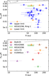 |
Fig. 2 Constraints on the vertical concentration of dust as a function of radius. Each symbol is associated with an horizontal bar corresponding to the range of radii over which the constraint was obtained. The gas scale height assumed in the modeling (Equation (1)) is indicated as a dashed gray line. Top: all disks. Bottom: five systems with both lower and upper limits on their dust height. |
4.2 Vertically thin outer disks in 18 systems
Similarly to previous studies, most systems included here only allow us to place upper limits on the acceptable value of the dust disk height. In the majority of cases, the best models correspond to those with the thinnest vertical extent (i.e., the weakest vertical turbulence αz,MCFOST). We show the major and minor axis profiles of the data and models in the regions where we obtained some constraints in Appendix D. The results are also summarized in Table A.2. In most cases, the upper limits on the dust height were obtained using the gap projection effect (see Sect. 3.1) either in a gap or in the outer edge of the disks.
Out of the 18 disks with only upper limits on their vertical height, only 3 allowed us to obtain different upper limits between the inner and outer regions of the disks. In AA Tau and AS209, the dust scale height is constrained to a smaller value in the outer regions than in the inner regions. On the other hand, the constraint in the outer ring of CI Tau is less strong than in its inner regions. In summary, no clear trend is obtained between the ring location and the upper limit on the dust scale height obtained for these systems (Fig. 2).
4.3 No constraints for 10 disks
While we selected disks with morphologies and orientations expected to be favorable for the study their vertical structures, a subsample of them do not allow us to place such constraints. Those are eight DSHARP targets (DoAr 33, Elias 20, Elias 27, HD 143006, SR 4, Sz 114, WaOph 6, WSB 52), one source from the Taurus survey (MWC 480), and DM Tau. These sources typically present lower inclinations and/or shallower gaps than in the rest of the sample, hence minimizing projection effects and preventing us from extracting information on their vertical structures. Additionally, we are unable to constrain the vertical distribution of the spiral disk Elias 27 because the gap interior to the spirals becomes deeper along the minor axis, which our radiative transfer model is unable to reproduce. This is likely caused by a true azimuthal variation in the dust density in this gap.
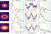 |
Fig. 3 Vertically thick inner ring and thin outer disk in HD 163296, LkCa 15, and V1094Sco. The shaded colors on the major axis cuts indicate the location of the azimuthal profiles (orange) and rings of interest (yellow and green). “Flat” models are too thin vertically to show sufficient azimuthal variation compared to the data (third panels), while “Thick” models are too vertically extended to reproduce the outer disk/ring brightness in all three disks (right panels). The beam size and a 25 au scale are indicated in the bottom left corner of the first panels. |
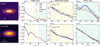 |
Fig. 4 Resolved thickness in the inner disk half and flat outer disk in DoAr 25 and HD 142666. For both disks, “Flat” models show too strong of a gap in the inner region (third panels), indicating that the disks must be thicker. On the other hand, “Moderate” and “Thick” models do not reproduce the gap and ring in DoAr 25, and the outer disk profile in both disks (last panels), highlighting the presence of a flat outer disk. The beam size and a 25 au scale are indicated in the bottom left corner of the first panels. |
4.4 Comparison with previous millimeter studies
The analysis presented in this work is new for 17 of the 33 disks of the sample. We extract new constraints on the dust vertical height for 13 of these 17 systems. The other ten disks for which we constrain the dust height have been previously modeled. Here, we compare our results with literature results for these ten disks.
Our results are consistent with the constraints obtained by Pinte et al. (2016) on HL Tau, who used the same prescription for vertical settling and devised the modeling approach used in the present work. However, the comparison of their results and our Table A.2 is not direct, because Pinte et al. (2016) report the height of 1 mm particles at a radius of 100au (H1mm = 0.7 au), while we report the height of the grains emitting the most at the observing wavelength, that is a ~ 59 μm in the case of HL Tau, at the location of the constraining region. Our constraints translate to H1mm ≤ 1.9 au at 100 au, which is in agreement with the results by Pinte et al. (2016), although less constraining. Another difference between the two works is also that they fitted observations at bands 3,6, and 7 together, while we only consider band 7 observations in this analysis. Our analysis is therefore sensitive to (less settled) smaller grains and higher optical depth, which could lead to a higher dust scale height. We also note the discrepancy in the reported αz,MCFOST of a factor about 7 between both studies. This is due to a difference in the total dust mass in both models, and allows us to highlight again that αz,MCFOST is a model-dependent estimate of the turbulence.
Our modeling of AS 209, Elias 24, GW Lup, MY Lup and Oph 163131 are consistent with constraints obtained in previous studies (Pizzati et al. 2023; Villenave et al. 2022). More specifically, we obtain similar upper limits for Elias 24 and the inner ring of AS 209 than in Pizzati et al. (2023). Our analysis of the second ring of AS209, GW Lup, and MY Lup however allows us to improve on the constraint limits placed by Pizzati et al. (2023) by a factor 1.4 to 3.1. This is due to the fact that our analysis now takes into account not only the minor axis profile but also different azimuthal directions. On the other hand, Villenave et al. (2022) obtained a smaller upper limit on the dust scale height of Oph163131 by a factor of about 2 compared to our result. This is because they exploit the unique geometry of this nearly edge-on system, focusing on the minor axis cut through the ‘ansae’ of the gap to estimate the vertical extent. In contrast, we employ a more general approach applicable to a wider range of systems.
In the case of HD 163296, our results slightly differ from the literature results. We obtain both a lower and an upper limit on the dust vertical scale height in the inner ring (0.006 ≤ Hd,R/R ≤ 0.067), while previous studies only constrained a lower limit on the scale height of this ring (Hd,R/R ≥ 0.056, Doi & Kataoka 2021; Liu et al. 2022). Because the lower limit obtained from previous studies is more constraining than our results, in the remaining of this study, we consider it as the lower limit on the dust scale height of HD 163296, such that: 0.056 ≤ Hd,R/R ≤ 0.067.
We note that six of the ten disks where our modeling does not allow us to obtain constraints were included in the sample of Pizzati et al. (2023, DSHARP disks without spirals). This work was also unable to estimate their vertical height using the gap projection effect. They empirically concluded that disks with an inclination of i > 25° and a gap depth lower than 0.65 are most favorable for constraining their vertical extent.
Previous studies at (sub)millimeter wavelengths already identified hints toward thicker inner disks in some of the systems considered here. For example, interior to the innermost gap of HD 142666, the minor axis profile presents an asymmetric brightness (previously pointed out by Jennings et al. 2022 and Ribas et al. 2024). These crescent-shaped asymmetries have been interpreted as being due to an optically thick wall (e.g, Ribas et al. 2024, Sect. 3.1), which is consistent with our finding of a finite dust height around the inner gap of this system.
Interestingly, Guerra-Alvarado et al. (2024) analyzed shorter wavelengths observations of HL Tau (band 9, 0.45 mm) and also identified a crescent feature, located around 32 au. They estimated that the scale height of the dust particles should be Hd,32/R > 0.08, which is significantly larger than our constraints at radii greater than 61au (Hd,R/R ≤ 0.041). This suggests that HL Tau might also be geometrically thicker in the inner regions than in the outer regions. Alternatively, the difference could be due to the fact that band 9 probes smaller grains than our band 7 observations, which are more vertically extended in the disk and have a larger optical depth than those detected in band 7. Similarly, our constraints on RY Tau at large radii (28–90 au, Hd,R/R ≤ 0.046) can be compared to the results of Ribas et al. (2024) who analyzed the required height of dust at 12 au to reproduce the wall effect observed in this system. Using radiative transfer modeling, they obtain Hd,12 = 0.2 au at 12 au, corresponding to Hd,12/R ~ 0.017. This value is consistent with our upper limit at radii larger than 28 au.
4.5 Comparison with scattered light observations
In this work, we find that five disks present a finite dust height in their inner region (i.e., measured or lower limit on the dust scale height) and an unresolved height in the outer disk. Three of them (HD 163296, LkCa 15, and V1094 Sco) definitively show that the inner ring has a thicker aspect ratio than the outer region. Such spatial variation in the disk thickness with radius, if also present for smaller particles, is expected to leave signatures on their scattered light images. Indeed, a thick inner region would cast a shadow to the outer disk, making it undetected at scattered light wavelengths.
Interestingly, these five disks have been observed with the VLT/SPHERE in scattered light. All disks are well detected and bright at near-infrared wavelengths. DoAr 25, HD 142666, and V1094 Sco show scattered light sizes comparable or larger than the millimeter dust emission, without clear substructures (Garufi et al. 2020, 2022) excluding disk self-shadowing. On the other hand, HD 163296 and LkCa 15 show a morphology clearly distinct from that of the continuum dust emission (Muro-Arena et al. 2018; Thalmann et al. 2016). In both cases, only the innermost ring is detected in scattered light, consistent with self-shadowing from the inner ring. Muro-Arena et al. (2018) modeled both the ALMA and SPHERE images of HD 163296. They showed that increased settling of the dust grains or depletion of small grains in the outer ring can explain the absence of outer ring in the scattered light images. In both HD 163296 and LkCa 15, the appearance of the scattered light images is thus suggestive of a thicker inner ring casting a shadow to the outer disk. Even though these studies consider very different grain sizes, this geometry is similar with what we inferred from the analysis of the 1.25 mm observations of these two systems. Detailed multi-wavelength modeling of these two systems could allow to further explore the physical relationship between the disk appearance in both wavelength ranges.
We also checked the ratio of near-infrared excess (NIR) to far-infrared excesses (FIR) for disks in our sample, as it could be indicative of some level of self-shadowing. Specifically, FIR-excesses less than 10% coupled with NIR excesses above 10% have been interpreted as evidence for self-shadowing (Garufi et al. 2024). We find that 16 disks in our sample have published estimates for both the near and the far infrared excess. Seven of them fall into the category of potentially self-shadowed systems (Garufi et al. 2018, 2022, 2024). Those are CI Tau, GW Lup, WSB52, DS Tau, and 3 of the sources where we identified a finite dust height in their inner regions at millimeter wavelengths: HD 142666, HD 163296, and LkCa 15. Besides, both DoAr25 and V1094Sco are bright in the near infrared and faint in the far infrared (Garufi et al. 2020), which would be consistent with the presence of a thicker inner region as found in our study.
5 Constraints on anisotropy of turbulence
5.1 Vertical dust-gas coupling
In Sect. 4, we showed that most outer disks are vertically thin, which suggests that vertical settling is occurring. Here, we aim to constrain the level of settling in the different regions. We estimate the ratio αz/St, which involves the level of vertical turbulence αz, and the Stokes number of the particles St characterizing the dust–gas coupling. Particles which are well mixed with the gas have a large ratio, while a low ratio (αz/St < 1) implies strong decoupling and significant vertical concentration. Assuming a balance between vertical stirring and settling, the ratio αz/St relates to the dust and the gas scale height, respectively Hd and Hg, following (e.g., Dubrulle et al. 1995):
![Mathematical equation: $\[\frac{\alpha_z}{\mathrm{St}}=\left[\left(\frac{H_{\mathrm{g}}}{H_{\mathrm{d}}}\right)^2-1\right]^{-1}.\]$](/articles/aa/full_html/2025/05/aa53822-25/aa53822-25-eq8.png) (5)
(5)
To estimate this ratio for all disks, we first estimate the gas scale height at the different ring locations. We report two scale heights and αz/St ratios in Table A.3 based on different assumptions, as is described below. On the one hand, we estimate Hg, model, the gas scale height as assumed in the modeling, which is using Equation (1). The corresponding αz/St|model ratio was obtained using this gas scale height.
On the other hand, we also estimate Hg, temp, the gas scale height obtained from the hydrostatic equilibrium using the midplane temperature of the models, T, following:
![Mathematical equation: $\[H_{\mathrm{g}, \text { temp }}(r)=\sqrt{\frac{k_{\mathrm{B}} T ~r^3}{G M_{\star} \mu m_{\mathrm{p}}}},\]$](/articles/aa/full_html/2025/05/aa53822-25/aa53822-25-eq9.png) (6)
(6)
with kB the Boltzmann constant, G the gravitational constant, M⋆ the stellar mass, μ = 2.3 the reduced mass, and mp the proton mass. To obtain the values reported in the second to last column in Table A.3, we consider the temperature of the most constraining model, averaged over the radial domain of the constraint. We find that the gas scale height obtained based on the hydrostatic equilibrium is systematically lower than the scale height assumed in the modeling, by up to a factor 2 lower. In addition, for each disk, we checked that the adopted Hg, temp agrees within 10% with the average scale height obtained using the temperature of the 4 models with different vertical thicknesses. We report the corresponding αz/St|temp ratio in Table A.3.
The top panel of Fig. 5 shows the most conservative values for the vertical αz/St in each region, ordered by increasing coupling. Nearly all disks/rings show αz/St < 1, which indicates that the grains are affected by vertical settling. Our results are consistent with those of previous studies (GW Lup, DoAr25, Elias24, AS209, MY Lup; HD 164296; Oph163131; Pizzati et al. 2023; Doi & Kataoka 2023; Villenave et al. 2022). Interestingly, however, some of the thick rings (HD 163296, V1094Sco, and LkCa 15) have lower limits on their αz/St ratio close to 1, indicating that settling is not efficient in these regions.
We then used these results to investigate potential correlations between the settling level, characterized by the ratio αz/St, and various disk or stellar parameters. As has already been shown in Fig. 2, there is no clear correlation between the radius and the local dust scale height between systems. Moreover, although we do not show the figures here, we also find no clear correlations with parameters such as accretion rates, dust masses, stellar masses, and the dust to stellar mass ratio. Specifically, we see that all disks with a finite dust scale height are spread across a wide range of accretion rates, dust and stellar masses (between 0.84 and 2.06 M⊙). Finally, we also note that our study includes 8 transition disks: AA Tau, GM Auriga, HD 163296, J1608, J1610, LkCa 15, PDS70, and RY Tau. Our sample, however, does not reveal significant differences between the level of vertical settling between the transition disks and the disks without a large central cavity. Similarly, the binary system Haro6-5B does not stand out from the rest of the sample, which is mostly composed of disks around single stars.
5.2 Radial dust–gas coupling
In the radial direction, at the location of dust rings, the equilibrium between dust drift and turbulent spreading also allows to relate a radial αr/St to the dust and gas radial width, respectively wd and wg (e.g., Dullemond et al. 2018):
![Mathematical equation: $\[\frac{\alpha_r}{\mathrm{St}}=\left[\left(\frac{w_{\mathrm{g}}}{w_{\mathrm{d}}}\right)^2-1\right]^{-1}.\]$](/articles/aa/full_html/2025/05/aa53822-25/aa53822-25-eq10.png) (7)
(7)
To estimate this ratio, we first evaluated the radial width of the dust rings. Previous studies aiming to constrain wd have either worked in the image plane (Dullemond et al. 2018), which is subject to uncertainties regarding the unconvolved width, or were performed using some visibility fitting (e.g., Jennings et al. 2022). Visibility fitting systematically reaches lower values than what was estimated from the image plane. Here, we took an alternative approach, where we consider the surface density profiles of the models as an unconvolved representation of the data. For each disk, we estimated the radial width of the rings by fitting a Gaussian to the rings in the final surface density profile obtained in the modeling (see Sect. 3).
The results are reported in Table A.4. We note that not all the rings for which a constraint in the vertical direction exists could also be constrained in the radial direction. In many cases, this is because the surface density profiles do not resemble a Gaussian, or because multiple rings are present in the unconvolved model to reproduce one single ring of the observations. The uncertainties reported in Table A.4 correspond to the standard deviation of the fit for all four models of each disk.
To estimate the αr/St ratio, we now need to estimate the radial width of the gas, wg. This could in principle be done directly by using molecular gas observations of the disks and tracing for deviation from Keplerian velocity. We use such constraints for the two disks studied by Rosotti et al. (2020): AS209 and HD 163296. However, such data are not always available for our sample and the complete analysis is out of the scope of this work. Instead, for the rest of the sample, we follow the simpler approach of Dullemond et al. (2018) in order to obtain a reasonable upper and lower limit for the radial width of the gas.
Under the assumption that the rings correspond to pressure bumps, the minimal size of the gas width has to be the gas scale height (e.g., Dullemond et al. 2018). We consider the local gas scale height as the lower limit for the gas radial width. Here, we only take into account the hydrostatic equilibrium gas scale height obtained using the model’s midplane temperature (wg, min = Hg, temp) because it is the lowest (see Table A.3) and thus provides the most conservative estimate for αr/St. On the other hand, following Dullemond et al. (2018), we assume that the distance from the peak of the ring to the deepest point in the gap inside of the ring is the upper limit for the gas width (wg, max). The results are reported in Table A.4.
We display the estimates for αr/St in the second panel of Fig. 5. Those were obtained for 21 rings, located in 15 disks (Table A.4). We find that 11 rings are consistent with radial dust trapping (αr/St < 1), while the other 10 rings do not necessarily require strong trapping. We find a good agreement in the resulting constraints for the dust rings in common between our sample and previous studies (AS209, Elias24, GW Lup; HD 163296; J1610; Dullemond et al. 2018; Rosotti et al. 2020; Jennings et al. 2022; Carvalho et al. 2024; Doi & Kataoka 2023; Facchini et al. 2020).
We are able to obtain a constraint on the radial trapping in only two vertically thick rings, in HD 163296 and LkCa 15 (using wd value from Facchini et al. 2020). In LkCa 15, the apparent dust width is larger than the gas scale height allowing us to only place a lower limit on the ratio αr/St. On the other hand, similarly to results from Doi & Kataoka (2023), we find that the inner ring of HD 163296 is subject to some radial trapping.
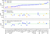 |
Fig. 5 Vertical αz/St (top), radial αr/St (middle), and their ratio αz/αr (bottom). In the bottom panel, we mark the rings without a full inclusion into the domain of the vertical constraints with a lighter blue. In all panels, constraints obtained by previous studies are shown in gray. The labels correspond to the constrained regions in Table A.3. The underscore ‘_1’ corresponds to the only or first region with a constraint in a disk, while ‘_2’ displays the results for the second region. |
5.3 Anisotropy of turbulence
We used our constraints on the vertical and radial dust-gas coupling to study the anisotropy of the turbulence in the different rings. In order to be conservative, we compared the least constraining αz/St from Table A.3 to αr/St from Table A.4. Because most constraints are upper limits in the vertical direction, we also mostly get upper limits on the ratio αz/αr. Moreover, we note that in some cases, the range of radii where the radial constraints (centered on the rings) were obtained do not fully overlap with that of the vertical constraints (centered on gaps). To increase the number of rings with an indication for the anisotropy of turbulence, we decided to include these systems, however marking them by a + in Table A.4 and with a lighter blue in Fig. 5. The results are reported in the last column of Table A.4 and shown in the third panel of Fig. 5.
We find that the upper limits for αz/αr vary between 0.06 and 8.57, with a median value of about 1.60. Out of the 20 rings, 7 have αz/αr ≲ 1, indicating that vertical turbulence is either weaker than radial turbulence within these rings (see also V4046 Sgr; Weber et al. 2022). On the other hand, similarly to Doi & Kataoka (2023), we find that vertical turbulence must be stronger than radial turbulence in the inner, vertically thick ring of HD 163296 located around 67 au. The other 12 rings do not allow to conclude on the anisotropy of turbulence and are consistent with vertical turbulence being either comparable to or weaker than radial turbulence.
5.4 Implications for the origin of turbulence
Our analysis indicated that most of the radial features in our sample are compatible with either quasi-isotropic turbulence (i.e., αz/αr ~ 1) or with features being disproportionately wider in the radial direction compared to their vertical extent (i.e., αz/αr < 1). Our estimates on the ratio αz/αr can then be used to constrain the mechanism driving the measured turbulence levels.
Specifically, our results suggest that the vertical shear instability (VSI, Nelson et al. 2013) is incompatible with most features, as it has been shown to drive highly anisotropic turbulence that manifests as vertically elongated motions with a vertical extent significantly larger than its radial counterpart (Nelson et al. 2013) and, consequently, αz ≳ 650αr ≫ αr (Stoll et al. 2017). It might still be possible for the VSI to be responsible for the vertical stirring of grains in some of the systems where our approach could not constrain αr, in which case a case-by-case analysis is necessary to examine whether the disk conditions can support the growth and saturation of the VSI at significant levels.
We note, however, that the VSI is commonly associated with an accretion stress or radial turbulence of αr ~ 10−5−10−3 (e.g., Stoll & Kley 2014; Manger et al. 2020), suggesting that a vertical turbulence of αz ≳ 10−2−10−1 is a reasonable expectation. Combined with typical Stokes numbers of St ~ 10−3−10−1 for millimeter-sized grains at R ~ 10–100 au scales (see also Sect. 6.1, Table A.5), we can narrow down the expected ratio αz/St to ≳ 0.1 for typical disk parameters. This in turn can rule out the VSI as the driving mechanism for several features where our analysis showed that αz/St ≲ 0.1 (highlighted in a light red region in the top panel of Fig. 5), even if a direct measurement of αz/αr was not possible. In addition, given that the strength of the VSI decays with increasing distance from the star as the dust–gas thermal coupling timescale renders cooling inefficient (thereby quenching the VSI, see e.g., Pfeil et al. 2023), we can argue that if a feature has been constrained to not be VSI-driven, any other features exterior to that in the same system are also unlikely to be VSI-related.
Nevertheless, we can identify different turbulence-driving mechanisms that are compatible with our results. In particular, for St ≲ 10−1, the emergent turbulence due to the streaming instability (SI, Youdin & Goodman 2005) tends to be isotropic between the radial and vertical directions even for an initial dust-to-gas ratio of order unity (e.g., Johansen & Youdin 2007; Baronett et al. 2024). Given that the majority of substructures analyzed here are compatible with radial dust trapping, which would naturally collect a high concentration of millimeter-sized grains with St ≲ 0.1, we expect that the SI could be operating in several of these rings. This concept has indeed been explored by other studies that suggest using the observed azimuthal variation in intensity to further constrain the extent to which the SI is taking place (e.g., Scardoni et al. 2024).
Another popular mechanism that is capable of both driving turbulence and creating the observed dust traps and substructure (rings, gaps) in the first place is, of course, embedded planets. The gravitational interaction between the planet and its surrounding disk gives rise to characteristic spiral waves (Ogilvie & Lubow 2002), which can deliver angular momentum into the disk (Rafikov 2002). Gap opening is then a natural byproduct of planet–disk interaction for even Saturn-mass planets in typical ALMA targets (more precisely, for a planet-to-star mass ratio of order ~(Hg/r)3, see Goodman & Rafikov 2001), with dust being efficiently trapped at the resulting outer gap edge. Three-dimensional models have further shown that planets excite both radial and meridional motion at the gap edge and around the excited spiral waves, which can in turn both lift dust above the midplane (Bi et al. 2021) and diffuse it radially about a dust trap (Bi et al. 2023). The resulting turbulent stresses αr and αz are of order ~10−3, suggesting that an assumption of αz/αr ~ 1 is not an unreasonable expectation.
Finally, it is possible for the origin of turbulence to lie in magnetohydrodynamic effects such as the ambipolar diffusion-mediated magnetorotational instability (Simon et al. 2013), which manifests as isotropic turbulent motion, or to the gravitational instability (GI, Toomre 1964; Kratter & Lodato 2016), which results in αr > αz (Béthune et al. 2021). However, the former would require the presence of a non-negligible vertical magnetic field, the strength of which is difficult to constrain observationally (e.g., Harrison et al. 2021), while the high disk masses required and the lack of observed spiral structures make the GI highly incompatible with most systems in our sample.
Overall, we expect the VSI to be incompatible with most of the systems in our sample, as we typically find that αz ≲ αr, while mechanisms such as the SI or planet–disk interaction are more favorable explanations for at least some of the observed substructures. Pinning down the dominant process that drives turbulence in each system would of course require a case-by-case analysis, which is beyond the scope of this study.
6 Constraints on turbulence level and implications
6.1 Estimating turbulence in the fragmentation limit
In this section, we attempt to break the degeneracy between St and α by assuming that the maximum grain size is limited by fragmentation. This is motivated by the results from laboratory experiments (Güttler et al. 2010; Beitz et al. 2011; Musiolik et al. 2016), which indicate that dust fragmentation can occur at low relative velocity, as low as tens of centimeter per second, depending on the dust composition. Observationally, multi-wavelengths observations have revealed relatively flat profiles for the maximum grain size as a function of radius in several disks (e.g., Sierra et al. 2021; Guidi et al. 2022). Performing numerical simulations of dust evolution in protoplanetary disks, Jiang et al. (2024) showed that this feature can be explained if dust growth is limited by fragmentation, with a fragmentation velocity of about 1 m s−1.
At the fragmentation barrier, the fragmentation threshold velocity vfrag can be equated with an approximate turbulent collision speed, such that the turbulent velocity coefficient αfrag and the fragmentation Stokes number Stfrag are related via the following (e.g., Birnstiel 2024):
![Mathematical equation: $\[\mathrm{St}_{\text {frag }}=\frac{1}{3 \alpha_{\text {frag }}}\left(\frac{v_{\text {frag }}}{c_{\mathrm{s}}}\right)^2.\]$](/articles/aa/full_html/2025/05/aa53822-25/aa53822-25-eq11.png) (8)
(8)
If the ratio ζ = α/St is known, Equation (8) can be rewritten as:
![Mathematical equation: $\[\alpha_{\text {frag }}=\frac{v_{\text {frag }}}{c_{\mathrm{s}}} \sqrt{\frac{\zeta}{3}}, \quad \mathrm{St}_{\text {frag }}=\frac{v_{\text {frag }}}{c_{\mathrm{s}}} \sqrt{\frac{1}{3 \zeta}},\]$](/articles/aa/full_html/2025/05/aa53822-25/aa53822-25-eq12.png) (9)
(9)
where ![Mathematical equation: $\[c_{\mathrm{s}}=\sqrt{\frac{k_{\mathrm{B}} T}{\mu m_{\mathrm{p}}}}\]$](/articles/aa/full_html/2025/05/aa53822-25/aa53822-25-eq13.png) is the disk sound speed. Contrary to the classical estimate of the Stokes number (e.g., Equation (3)), the above formulations allow us to estimate the fragmentation turbulence level and Stokes number without any assumptions on the relevant dust size and gas density.
is the disk sound speed. Contrary to the classical estimate of the Stokes number (e.g., Equation (3)), the above formulations allow us to estimate the fragmentation turbulence level and Stokes number without any assumptions on the relevant dust size and gas density.
We estimated αfrag and Stfrag using Equation (9). We assumed a fragmentation velocity of vfrag = 1 ms−1, and used ζ = αz/St; that is, the value for the vertical dust–gas coupling as constrained in Sect. 5.1 (Table A.3). Effectively, this assumes that vertical turbulence is dominant over, or comparable to radial turbulence. This is a reasonable assumption, as only a limited number of rings analyzed in Sect. 5.3 display a notably different relative turbulence strength (only 4/20 rings with αz < 0.2αr, and 1 with αz < 0.1αr). To estimate the disk sound speed, we considered the midplane temperature in the mcfost models, averaged over the radial domain of the constraint (see Sect. 5.1). We report the results in Table A.5, in addition to the assumed values in the mcfost models.
We find that the turbulence level obtained assuming the fragmentation limit αfrag reaches upper limits between 1.7 × 10⁻⁴ and 5.8 × 10⁻³, with a median of 1.1 × 10⁻³ (Table A.5). These estimates are almost systematically lower than their assumed values in the mcfost models, with an average difference of a factor about 2. Consequently, the Stokes numbers obtained assuming the fragmentation limit are also systematically lower than what is assumed in the mcfost models (see Table A.5, Appendix C), suggesting that the disk masses (or grain sizes) in mcfost may be too low (or too high) by a similar factor (see Equation (3)).
Five disks in our sample were previously included in the study of Jiang et al. (2024), who estimated αfrag for the same fragmentation velocity, using disk masses inferred from optically thin dust emission and a gas-to-dust ratio of 100, and considering the maximum dust size inferred from existing multi-wavelengths analysis. We find that our results are consistent with their findings as, in most cases, the values inferred by Jiang et al. (2024) are lower than the upper limits obtained here. Zagaria et al. (2023) used an alternative method to estimate the turbulence in HD163296 in the fragmentation limited regime. They used the observed dust sizes and midplane temperature obtained from multi-wavelengths observations combined with an estimate of αr/St to infer αfrag. The turbulence value that they obtained for the outer ring is consistent with our estimate, while their lower limit for the turbulence in the inner ring is about 4 times larger than our estimate.
6.2 Comparison with accretion turbulence
Historically, turbulence was introduced as a way to explain the observational fact that disks accrete. Since the mechanism producing turbulence was not known at the time when disks were postulated to be turbulent, and its exact nature is still elusive many decades after, it has become common to adopt a single value for the turbulence strength α, assuming this applies to the entire disk. While angular momentum transport and therefore accretion are influenced mostly by radial turbulence, it is also common to assume that turbulence is isotropic and therefore the radial and vertical values of α are the same.
In the previous sections however, we showed that the strength of turbulence can be different in the vertical and radial directions, with seven cases of stronger radial turbulence than vertical turbulence, and 13 rings where the opposite cannot be excluded (Fig. 5). Now, we aim to compare the level of vertical turbulence αfrag, which we estimated assuming that dust size is limited by fragmentation (Sect. 6.1), to the level of turbulence which can be expected based on the accretion rate of the disks (hereafter accretion turbulence or αacc).
Using disk global quantities, the accretion turbulence is related to the mass accretion rate, ![Mathematical equation: $\[\dot{M}\]$](/articles/aa/full_html/2025/05/aa53822-25/aa53822-25-eq14.png) , and the total disk mass, Mdisk, following (e.g., Rosotti 2023):
, and the total disk mass, Mdisk, following (e.g., Rosotti 2023):
![Mathematical equation: $\[\alpha_{\mathrm{acc}}=\frac{\dot{M}}{M_{\text {disk }}} \frac{\mu m_{\mathrm{p}}}{k_{\mathrm{B}} T} \Omega R_{\mathrm{c}}^2,\]$](/articles/aa/full_html/2025/05/aa53822-25/aa53822-25-eq15.png) (10)
(10)
where μ, mp, kB, T have already been defined in Sect. 5.1, ![Mathematical equation: $\[\Omega= \sqrt{G M_{\star} / R_{\mathrm{c}}^{3}}\]$](/articles/aa/full_html/2025/05/aa53822-25/aa53822-25-eq16.png) , and Rc is a length-scale describing the disk size, that is, within which a significant fraction of its mass resides. This length-scale can be quantified using commonly used analytical functional forms for the disk surface density (Lynden-Bell & Pringle 1974).
, and Rc is a length-scale describing the disk size, that is, within which a significant fraction of its mass resides. This length-scale can be quantified using commonly used analytical functional forms for the disk surface density (Lynden-Bell & Pringle 1974).
We remark that this formula is the most empirical estimate of accretion turbulence we can make; it does not prove in any way that disks are turbulent, but it quantifies how turbulent disks should be if accretion is indeed powered by turbulence. If this is not the case, the formula is still useful as it quantifies how effective angular momentum transport processes are. Finally, we note that we use global quantities here rather than local (e.g., disk mass rather than the disk surface density at the ring location) because those would require to make the further assumption that the disk is in steady state. Given the large radii of many of the rings we considered in this study, this is unlikely to be the case.
As with any estimate, the reliability of the values returned by Equation (10) depends on the reliability of the values used as input. Several attempts were made in the literature to estimate the accretion turbulence, starting from the seminal work of Hartmann et al. (1998). One of the main variable in these studies is the assumed disk radius. For example Rafikov (2017) used the millimeter continuum dust sizes to estimate αacc, while Ansdell et al. (2018) considered the observed 12CO size. As was stated above, the disk radius should instead be linked to where most of the disk mass is. Many works have shown that the dust radius fails to represent most of the gas mass due to radial drift; on the other hand, the 12CO size is not a good indicator either due to the high CO optical depth, which leads to an overestimate of Rc. To ensure we have accurate estimates, we restrict our sample and consider here studies where the disk radius has been determined by two techniques. The first consists in fitting the disk rotation curve (Martire et al. 2024 for AS209, GM Aur, HD163296; and Longarini et al. 2025, based on Izquierdo et al. 2025, Galloway-Sprietma et al. 2025, and Stadler et al. 2025 for LkCa 15), which directly probes the disk radius through its mass. The second technique consists in using thermochemical models to derive the physical size from the observed 12CO size (Trapman et al. 2023, for the rest of the sample).
The other variable to discuss is the disk mass. Dust based estimates are available for all our disks, but we opt not to use them as these are highly dependent on the assumed dust-to-gas ratio. Instead, we restrict the sample to disks where the gas mass has been estimated through the rotation curve, in the same way as the disk size (Martire et al. 2024; Longarini et al. 2025, for AS209, GM Aur, HD 163296, LkCa 15), or alternatively from CO gas line observations. In this latter case, since these estimates are dependent on the CO abundance, we only consider cases where the CO abundance could be inferred from combined N2H+ observations (Trapman & AGE PRO team 2025, for GW Lup and V1094Sco), or safely assumed because the source is a Herbig star (Stapper et al. 2024, for HD 142666), for which the consensus is that they should have ISM-like levels of CO abundance. Finally, we note that we assume a disk temperature at Rc based on our mcfost models.
The results are shown in the top panel of Fig. 6. We find accretion turbulence levels between 3.0 × 10⁻⁴ and 2.0 × 10⁻², with a median of 3.0 × 10⁻³. Our values appear to be in line with the results of Ansdell et al. (2018). As was mentioned before, we note however that using the observed 12CO size the authors likely overestimated accretion turbulence. This could mean the sample we consider here is biased toward high accretors. Pending confirmation on a larger statistical sample where αacc is estimated in a uniform and reliable way, if this is true this would make our sample a natural one where to search for turbulence and establish if it drives accretion.
Comparing αacc with αfrag (Fig. 6, Table A.5), we find that, in 8 cases out of 14, the upper limits on turbulence we put in this paper are lower than what is required to drive accretion. At face value, this implies that in those disks turbulence is too small to explain the accretion rates we measure and therefore accretion is not driven by turbulence, or that the rings and gaps we studied in this work have a lower turbulence than the bulk of the disk. It should be remarked however that this is a strong statement only for AS 209, and region 2 of HD 163296, where αfrag is significant lower than αacc – the other cases are only a marginal mismatch. Conversely, for 6 cases out of 14, a mix of upper and lower limits, we find that our results are compatible with turbulence-driven accretion. In one case, region 1 of LkCa 15, the turbulence we detect is even too high to explain accretion, implying that the local value we measure is probably significantly higher than in the rest of the disk. Overall, our results do not allow us to make strong conclusions regarding whether accretion is driven by turbulence at a population level, though it is significant that we find a few sources where turbulence seems unable to power accretion. We remark that at the population level this is a different outcome from a similar analysis in HL Tau (Pinte et al. 2016) and highlights the importance of conducting these studies for a sample.
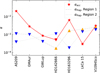 |
Fig. 6 Comparison between accretion turbulence (in red) and the fragmentation turbulence αfrag, derived from ζ = αz/St (Sect. 6.1). |
7 Implications for planet formation and limitations
7.1 Implications for wide-orbit planet formation
In the core accretion scenario, giant planets form by first accreting an approximately ten-Earth-mass solid core within the gas disk lifetime (Mizuno 1980; Pollack et al. 1996). This is challenging in wide-orbits given the relatively short lifetimes of protoplanetary disks of a few million years, determined from the rapidly decreasing solid mass budget in nearby star-forming regions (Ansdell et al. 2017; Michel et al. 2021; Manara et al. 2023). Despite this formation timescale challenge, wide-orbit giant planets are a relatively common type of planet with an approximate occurrence rate of between 5 and 10% percent around solar-mass stars (Nielsen et al. 2019; Fulton et al. 2021; Vigan et al. 2021). Moreover, the frequently observed dust rings in large protoplanetary disks, as explored in this work, could be consistent with a population of wide-orbit planets in the process of completing their growth (Zhang et al. 2018; Ruzza et al. 2024).
Core growth in wide orbits is maximally efficient when planetary embryos can accrete small pebbles (Lambrechts & Johansen 2012), because small dust particles approximately millimeter in size experience gas drag which increases the accretion cross section (Ormel & Klahr 2010). However, pebble accretion critically relies on pebbles settling toward the disk midplane. In order to assess which disk regions could be prone to drive core growth via pebble accretion, and which ones can crudely be ruled out, we can express a core formation time
![Mathematical equation: $\[t_{\mathrm{acc}, 3 \mathrm{D}}=\frac{M_{\mathrm{c}}}{\dot{M}_{c, 3 D}},\]$](/articles/aa/full_html/2025/05/aa53822-25/aa53822-25-eq17.png) (11)
(11)
where ![Mathematical equation: $\[\dot{M}_{c, 3 D}\]$](/articles/aa/full_html/2025/05/aa53822-25/aa53822-25-eq18.png) is the so-called 3D accretion rate onto an embryo of mass Mc. This 3D accretion regime is valid when the accretion cross section is smaller than the pebble scale height Hp and is appropriate to describe the critical growth regime from planetesimal to larger embryos growing in the more efficient 2D pebble accretion regime.
is the so-called 3D accretion rate onto an embryo of mass Mc. This 3D accretion regime is valid when the accretion cross section is smaller than the pebble scale height Hp and is appropriate to describe the critical growth regime from planetesimal to larger embryos growing in the more efficient 2D pebble accretion regime.
In this 3D growth phase, the accretion rate is proportional to the embryo mass, resulting in a mass-independent growth timescale that only depends on the particle Stokes number through the pebble disk aspect ratio (Hp/r):
![Mathematical equation: $\[t_{\mathrm{acc}, 3 \mathrm{D}} \approx \eta \frac{H_{\mathrm{p}}}{r} F^{-1} M_{\star},\]$](/articles/aa/full_html/2025/05/aa53822-25/aa53822-25-eq19.png) (12)
(12)
for a given pebble flux, F (Lambrechts & Johansen 2014), and where η here is a measure that expresses the pressure support in the disk (Nakagawa et al. 1986).
Making the same assumption as in Sect. 6.1, namely that pebbles are fragmentation limited, we can rewrite the pebble flux driven by radial drift in the Epstein regime, to obtain:
![Mathematical equation: $\[t_{\mathrm{acc}, 3 \mathrm{D}} \approx\left(r \Sigma_{\mathrm{p}}\right)^{-1}\left(\frac{H_p}{r}\right)^2 v_{\mathrm{frag}}^{-1} M_{\star},\]$](/articles/aa/full_html/2025/05/aa53822-25/aa53822-25-eq20.png) (13)
(13)
where Σp is the pebble surface density and vfrag is the pebble fragmentation velocity. In this way, we obtain an expression where the pebble accretion timescale is fully determined by two observable quantities, the pebble aspect ratio and surface density. Finally, we can rewrite Equation (13) to express the critical pebble scale height needed for core growth timescales within disk lifetimes:
![Mathematical equation: $\[\begin{gathered}\left.\frac{H_p}{r}\right|_{\text {crit }} \approx 0.033\left(\frac{r}{100 ~\mathrm{au}}\right)^{1 / 2}\left(\frac{v_{\text {frag }}}{1 \mathrm{~ms}^{-1}}\right)^{1 / 2}\left(\frac{t_{\mathrm{acc}, 3 \mathrm{D}}}{1 ~\mathrm{Myr}}\right)^{1 / 2} \\\\\left(\frac{\Sigma_{\mathrm{p}}}{0.1 \mathrm{~g} / \mathrm{cm}^2}\right)^{1 / 2}\left(\frac{M_{\star}}{M_{\odot}}\right)^{-1 / 2}.\end{gathered}\]$](/articles/aa/full_html/2025/05/aa53822-25/aa53822-25-eq21.png) (14)
(14)
Here, we set the core growth timescale to tacc,3D to a characteristic disk age value of tacc,3D = 1 Myr and assume solar-mass stars. The dependency of the critical pebble disk aspect ratio on the local pebble surface density is illustrated in Fig. 7.
Several of the modeled disk regions have upper limits on the dust scale height that would allow core formation to proceed efficiently even at wide orbital distances outside of 50 au. Fig. 7 shows the observational constraints on the dust aspect ratio and dust surface density for all disks in this study (see Table A.2) that can be compared with the critical pebble scale height of Equation (14). We show both the peak and median surface densities in each region, as obtained in Sect. 3.3, with respectively large and small triangle symbols.
In particular, the protoplanetary disk AS 209 stands out: both ring at 74 au and 120 au (see Fig. D.2) have upper limits on the dust aspect ratio that place it in a region of parameter space where core growth by pebble accretion would be possible. Similarly, the disk DoAr 25 (Fig. 4) contains two dust rings suitable for core growth by pebble accretion. Finally, the low dust scale height in the outer ring of HD 163296 (Fig. 3) makes it a region possibly prone to core growth even at 100 au distances. Interestingly, the above disks are also suspected to host wide-orbit planets, based on kinematic perturbations in CO emission: around 200 au in AS 209 (Bae et al. 2022), in the gap at 98 au around DoAr 25 (Pinte et al. 2020), and around 83 and 137 au in HD 163296 (Teague et al. 2018; Pinte et al. 2018b; Izquierdo et al. 2022). Therefore, it remains currently difficult to disentangle if these dust rings were the seeding grounds for core formation, or reflect current pile-up regions after giant planets already formed that are perhaps still prone to ongoing planet formation.
Some of the obtained lower-limits on dust scale heights already effectively rule out specific regions as sites for efficient core growth (upward triangles in the shaded purple area of Fig. 7). Two exceptions to this are the lower-limits given for the inner rings in the disks of Doar 25 and HD 142666, the latter being the most close-in region probed in this study (≲50 au, Fig. 4). In general, the current data is consistent with a possible trend of increased dust scale heights closer to the host star (bottom panel of Fig. 2, Sect. 4.1). If this holds, the inner disk, crudely within half the dust radius, would be less conductive to core growth by pebble accretion. This is because the growth timescale expressed in Equation (13) mainly depends on the pebble scale height: the factor rΣp is nearly constant, if Σp approximately follows a nominal gas disk scaling Σg ∝ r−1. In a broader perspective, this finding appears to be consistent with previous works proposing that giant planet formation is initiated in the outer disk, after which planets migrate inward, complete their growth and form the basis of the observed population of warm and cold Jupiter exoplanets. This has been argued on the basis of theoretical population synthesis models (Lodato et al. 2019; Ndugu et al. 2019) and disk substructure/exoplanet statistical analysis (van der Marel & Mulders 2021).
We have here presented an initial exploration to identify low pebble-scale-height disks with adequate pebble surface densities to be potential sites of pebble-accreting cores. Following works could target disks for more in-depth modeling and to verify that the fragmentation-limit assumed here holds by determining pebble sizes. This appears at least to be the case for AS 209 and HD 163296 (Jiang et al. 2024). A more detailed study could also explore the core formation process in more detail, fine-tuned per disk, by considering core growth from a pebble-dense planetesimal-forming region and subsequent inward migration. In that context, pebble accretion in pebble-rich rings can be highly efficient (Jiang & Ormel 2023), unless a pressure-bump generated pebble ring contains only a limiting finite mass reservoir (Morbidelli 2020).
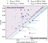 |
Fig. 7 Critical dust surface density for core formation by pebble accretion as function of the solid surface density. Large and small symbols indicate, respectively, the peak and median dust surface density for each of the modeled disk regions, while upper- and lower-limits on the dust disk aspect ratios are indicated by, respectively, downward and upward triangles. The ring location is color-coded according to orbital distance (see legend). The gray lines connecting triangles highlight two regions within the same disk. The figure area below the dashed green line marks rapid core growth timescales: below 1 Myr at 50 au in the 3 D pebble accretion regime, assuming fragmentation-limited pebbles (see Sect. 7). The dashed purple line illustrates the 1-Myr-core-growth timescale at 100 au. Disk regions with aspect ratios in the shaded purple region are unlikely to form planetary cores within disk lifetimes. |
7.2 Caveats and future prospects
This section discusses some caveats regarding the different aspects of this work, starting with observational considerations and moving toward more modeling related points. Some observational characteristics are not reproduced by our radiative transfer model. While these are located in regions where we do not put any constraints on the dust height, we point them out here because they could be interesting to study in future works. For example, several systems show deeper gaps along the minor axis than along the major axis direction (e.g., Elias27). In some cases (e.g., DL Tau, HL Tau, and V1094Sco) a ring which is well visible along the major axis direction completely disappears in the minor axis profile. In HL Tau (ring between 64–74 au), this has previously been pointed out by Pinte et al. (2016). This effect is in appearance similar to the ring effect previously discussed in Sect. 3.1. However, in all of these systems, even our thickest models are not able to reproduce the depth of the gap along the minor axis direction. For example, in the case of V1094Sco (Fig. 3), all models are similar between 164 and 201 au and do not reproduce the gap in the data well. Further modeling would be required to fully understand the origins of this behavior.
Moreover, a few systems (CI Tau, ISO-Oph17, and J1610) show a surprising azimuthal variation in their brightness profiles, with the disk being brighter along the minor axis direction than along its major axis. This is not expected to be caused by projection effects and is not well reproduced by our radiative transfer models. We hypothesize that in some cases, these rings could be partially optically thick and that the effect detected here could be similar to that reported by Scardoni et al. (2024).
We note here the degeneracy between the optical thickness and the true scale height. From the apparent vertical thickness, we assumed a reasonable optical thickness (surface density and dust properties) to estimate the dust scale height. However, we note that other combinations of optical thickness and dust scale height might be possible. Moreover, the dust heights reported in Table A.2 were obtained by fitting a Gaussian function to the vertical density profile of one dust size only, corresponding to dust with the maximum opacity at the wavelength of the observations (see Sect. 3.5). We caveat however that the true vertical profile of the dust is not exactly a Gaussian (see Equation (2)), and that several dust sizes might be contributing to the final image resulting from radiative transfer modeling.
For completeness, we also note that we assumed a constant dust-to-gas ratio radially throughout the disk. While we separate the inner and outer regions of the disk during our analysis, we note that the models do not include radially variable settling. We caveat that some effects of varying settling between the inner and outer regions, such as shadowing, cannot be captured under this assumptions. Furthermore, the settling prescription we assume supposes that the vertical density profile of the gas follows a Gaussian, that diffusion is constant vertically, and that there is no feedback of dust to the gas. Regarding the latter point, Lim et al. (2024) showed that the level of turbulence inferred by ignoring feedback (here, the model dependent αz,MCFOST) is potentially lower than that required in case where dust interacts with gas.
While we estimated the gas scale heights under the assumption of hydrostatic equilibrium (using Equation (6)), direct observational constraints to the gas scale height would be valuable to better estimate the ratio Hd/Hg and more precisely determine the ratio αz/St. This could for example be done by first determining the emitting surfaces of molecules (Pinte et al. 2018a; Law et al. 2021) and then retrieving the gas scale height using thermochemical modeling or analytical expressions (e.g. Paneque-Carreño et al. 2023).
The estimate of αr/St is based on the assumption that the rings correspond to pressure maxima. However, only two systems in our sample have direct evidences that this is the case, with a direct measurement of the gas radial width (wg) using molecular line emission (Rosotti et al. 2020). Expanding on the sample of rings with such direct estimates would also allow us to critically improve on our evaluation of αr/St, and thus on the anisotropy of turbulence at various locations. This could be done with the observations of the exoALMA large program.
Finally, the determination of αfrag depends on several assumptions which we state again here. First we assumed that the dust size is limited by fragmentation. This seems reasonable given the relatively low variation in the maximum grain size between the location of rings and gaps in different systems observed with multi-wavelengths observations (Sierra et al. 2021; Jiang et al. 2024) but might be incorrect in the outer disks where the grain size could be limited by radial drift instead. Further, we used our estimates of αz/St to obtain αfrag, which effectively assumes that vertical turbulence is dominant, and we assumed a low fragmentation velocity of 1 ms−1, as done in previous studies (Jiang et al. 2024) and consistent with some laboratory experimental results (Güttler et al. 2010). In the case where the fragmentation velocity was larger or if vertical turbulence did not dominate we would expect the values of αfrag to become higher. This could affect the discussion of Sect. 6.2, by changing the relative ratio between αfrag/αacc in some disks where αfrag is only marginally smaller than αacc.
8 Conclusions
We produced radiative transfer models of 33 inclined and ringed protoplanetary disks with high quality observations in the ALMA archive, aiming to constrain the vertical extent of the particles emitting in band 6 (1.3 mm) or band 7 (0.9 mm). Our analysis of the observations leads to the following results:
10 disks do not allow us to provide significant constraints on the local dust scale height;
We provide upper limits on the dust scale height for the outer regions of the 23 remaining disks;
For 5 disks, we also obtain a lower limit on the dust scale height in the region within approximately half of the disk radius. Three of them (HD 163296, LkCa 15, and V1094Sco), definitely exhibit a thicker aspect ratio in the inner ring than in the outer disk;
By comparing the measured dust scale height with estimated gas scale heights, we evaluate the vertical ratio αz/St. We find that vertical settling is prominent in most systems, as is indicated by low values of αz/St < 1;
Three systems (HD 163296, LkCa 15, and V1094Sco) showed evidence of enhanced mixing in their inner regions;
We also estimate the radial ratio αr/St of several rings by comparing the locally estimated gas scale heights with the dust widths. We find that αr/St < 1 for 11 rings, consistent with radial trapping, while the other 10 rings do not necessitate strong trapping.
We explored the implications of our findings on dust settling and radial trapping for the anisotropy of turbulence, its origin, disk evolution, and planet formation. Our key results include:
The analysis of 20 rings reveals that vertical turbulence is typically comparable to or weaker than radial turbulence (αz ≲ αr). The inner ring of HD 163296 is a notable exception, displaying stronger vertical than radial turbulence, in agreement with previous studies;
The apparent turbulence anisotropy suggests that VSI is incompatible with most of the rings in our sample, as it produces strong vertical and weak radial turbulence. Mechanisms like the streaming instability or planet-disk interaction may better explain some of the observed substructures;
Aiming to disentangle α and St, we assume that the dust size is limited by fragmentation, with a fragmentation velocity of 1 m s−1. We use our estimate of αz/St to estimate αfrag and Stfrag without assumption on the relevant dust size and gas density. We find a median upper limit of αfrag ≲ 1.1 × 10⁻³;
We compared αfrag to the turbulence level required for accretion in seven disks with well-constrained gas disk properties (gas size and gas mass); Although we cannot make strong conclusions regarding the link between accretion and turbulence across all disks, we find few sources where the inferred turbulence cannot be the main source of accretion;
Finally, we analyzed our estimates for the dust scale height and dust surface densities in the context of pebble accretion. We find that several of the modeled disk regions have estimates that would allow core formation to proceed efficiently within about 1 Myr, even at wide orbital distances outside of 50 au. In the case of the disks with vertically thicker inner than outer disk, we find that planet formation could be faster in the outer disk.
This highlights the need for a better understanding of the physical structure of the disk and dust vertical settling across all radii to better comprehend the best locations for forming planets.
Data availability
The data can be found on zenodo (zenodo.14054952). The models are also available (zenodo.14056832).
Acknowledgements
We thank the referee for their review of the manuscript, and Fabiola Gerosa for spotting a major typo in a final stage of the manuscript. The authors thank the DSHARP team and Jane Huang for making their calibrated visibilities and imaging scripts publicly available. We also thank Feng Long, Myriam Benisty, Jun Hashimoto, and Álvaro Ribas for sharing some of the calibrated visibilities used in this work, and the NRAO SRDP and ESO ARI-L (Massardi et al. 2021) for providing calibrated visibility files. We thank Giuseppe Lodato for very useful discussions. MV and GR acknowledge support from the European Union (grant No. 101039651, project DiscEvol) and from Fondazione Cariplo (grant No. 2022-1217). FMe and GD acknowledge funding from the European Research Council (ERC) under the European Union’s Horizon Europe research and innovation program (grant agreement No. 101053020, project Dust2Planets). AZ acknowledges funding by the STFC (grant ST/P000592/1), and from the European Union under the European Union’s Horizon Europe Research and Innovation Programme 101124282 (EARLYBIRD). ML acknowledges ERC starting grant 101041466-EXODOSS. Views and opinions expressed are, however, those of the author(s) only and do not necessarily reflect those of the European Union or the European Research Council. Neither the European Union nor the granting authority can be held responsible for them. This paper makes use of the following ALMA data: 2013.1.00498.S, 2015.1.00888.S, 2016.1.00484.L, 2016.1.00460.S, 2016.1.00545.S, 2016.1.00771.S, 2016.1.01164.S, 2016.1.01205.S, 2016.1.01239.S, 2016.1.01370.S, 2017.A.00006.S, 2017.1.01151.S, 2017.1.01167.S, 2017.1.01460.S, 2018.1.00028.S, 2018.A.00030.S, 2018.1.00689.S, 2018.1.00958.S, 2018.1.01255.S, 2018.1.01230.S, 2018.1.01755.S, 2019.1.01051.S. ALMA is a partnership of ESO (representing its member states), NSF (USA), and NINS (Japan), together with NRC (Canada), MOST and ASIAA (Taiwan), and KASI (Republic of Korea), in cooperation with the Republic of Chile. The Joint ALMA Observatory is operated by ESO, AUI/NRAO, and NAOJ. This paper used the following softwares CASA (CASA Team 2022), mcfost (Pinte et al. 2006, 2009), Matplotlib (Hunter 2007), Numpy (Harris et al. 2020), scipy (Virtanen et al. 2020), CARTA (10.5281/zenodo.3377984).
Appendix A Tables
We present here the main tables including the results of this paper. Table A.1 gathers the disk and stellar parameters considered for this study. Table A.2 presents the vertical constraints obtained in the different disk regions, the corresponding grain size for which they are valid, and the local and total dust mass in the models. Table A.3 shows the implications of these results for vertical trapping. Table A.4 indicates the level of radial trapping and turbulence anisotropy. Finally, Table A.5 compares αMCFOST assumed in the radiative transfer modeling with αfrag assumed based on the vertical constraints and assuming fragmentation limited dust (Sect 6.1). αacc estimated to explain the level of accretion in a few systems (Sect. 6.2) is also reported in Table A.5.
Disk parameters assumed in our modeling.
Constraints on the dust vertical concentration in different radial domains, local dust mass, and total dust mass.
Vertical trapping.
Radial trapping and anisotropy of turbulence.
α and St assumed in the models, derived based on fragmentation limited dust sizes, or to explain accretion.
Appendix B Observational parameters
We present the characteristics of the archival observations that we have used for this work. We have modeled a total of 33 protoplanetary disks. In Table B.1, we report the project IDs, beam size and wavelengths of the observations of the 23 sources where some constraints on their level of vertical turbulence could be obtained. On the other hand, Table B.2 shows the same characteristics for the other disks modeled during this project but where no constraints have been obtained. When no constraints could be obtained, the disks were either not very inclined, possessed only shallow substructures, or the presence of spiral interior to the gap of interest made the interpretation of the model incorrect.
Sample and image properties of the disks with constraints on their vertical thickness.
Sample and image properties of the disks without constraints on their vertical thickness.
Appendix C Comparison of Stfrag with StMCFOST
In Fig. C.1, we show how the assumed Stokes number in our mcfost models compares with the estimated Stokes number assuming grain growth is limited by fragmentation. We assumed a fragmentation velocity of 1 m s−1 and used the observational constraints on ζ = αz/St to obtain Stfrag (see Sect. 6.1). Stfrag is nearly systematically lower than StMCFOST suggesting that the disk masses obtained with our iterative fitting of the surface density in mcfost may be too low.
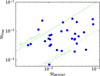
Appendix D Cuts and metric estimates
In Fig. D.1, we show images and metrics for the five disks for which we find that the inner disk half shows a finite dust thickness while the outer disk is settled (Sect. 4.1). In Fig. D.2, Fig. D.3, and Fig. D.4, we present an overview of the 18 disks for which only upper limits on their vertical thickness could be obtained (Sect. 4.2). For all models, we also show the values of χ2 and 𝒮 (Sect. 3.4).
We remind the reader that the normalized χ2 corresponds to the average of ![Mathematical equation: $\[\chi_{azimuth}^{2} / \chi_{majorAxis}^{2}\]$](/articles/aa/full_html/2025/05/aa53822-25/aa53822-25-eq23.png) over each azimuthal direction. On the other hand 𝒮, estimates the Hausdorff distance, which takes into account the likelihood in shape between the model and the data. By visual inspection, we identify that models with χ2 ≤ 8 and 𝒮 ≤ 1.2 are generally good models. However, we always perform a visual check before reporting the value in Table A.2 and in some rare cases, the reported values might be slightly different from those highlighted by the metrics.
over each azimuthal direction. On the other hand 𝒮, estimates the Hausdorff distance, which takes into account the likelihood in shape between the model and the data. By visual inspection, we identify that models with χ2 ≤ 8 and 𝒮 ≤ 1.2 are generally good models. However, we always perform a visual check before reporting the value in Table A.2 and in some rare cases, the reported values might be slightly different from those highlighted by the metrics.
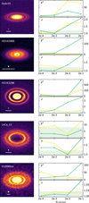 |
Fig. D.1 Left: Data image, Right: Values for the χ2 and shape parameter 𝒮 (Sect. 3.4), quantifying the quality of the models. The green regions indicate that the models are generally good models. Yellow curves indicate results for the inner ring/region while green curves show that for the second ring/region. Major axis profiles highlighting the radial location of the different regions are shown in Fig. 3 and Fig. 4. The beam size and a 25 au scale are indicated in the bottom left corner of the first panels. |
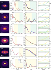 |
Fig. D.2 Left: Data image, Middle left: Major axis profiles of the data and models outside of 5au. Middle right: Profiles along an azimuth of the data and model, zoomed in the constrained region. Right: Values for the normalized χ2 (top) and shape parameter 𝒮 (bottom), introduced in Sect. 3.4, quantifying the quality of the models. The green regions indicate that the models are generally good models. The colors of the curves correspond to the similarly colored range of radius in the major axis profile displayed in the second left panel. The beam size and a 25 au scale are indicated in the bottom left corner of the first panels. |
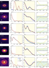 |
Fig. D.3 Same as Fig. D.2. For GM Aur, χ2 is artificially higher for model 2e-4 because |
![Mathematical equation: $\[\chi_{majorAxis}^{2}\]$](/articles/aa/full_html/2025/05/aa53822-25/aa53822-25-eq24.png)
References
- Alcalá, J. M., Manara, C. F., Natta, A., et al. 2017, A&A, 600, A20 [NASA ADS] [CrossRef] [EDP Sciences] [Google Scholar]
- Andrews, S. M., Huang, J., Pérez, L. M., et al. 2018, ApJ, 869, L41 [NASA ADS] [CrossRef] [Google Scholar]
- Angelo, I., Duchene, G., Stapelfeldt, K., et al. 2023, ApJ, 945, 130 [NASA ADS] [CrossRef] [Google Scholar]
- Ansdell, M., Williams, J. P., Manara, C. F., et al. 2017, AJ, 153, 240 [Google Scholar]
- Ansdell, M., Williams, J. P., Trapman, L., et al. 2018, ApJ, 859, 21 [NASA ADS] [CrossRef] [Google Scholar]
- Bai, X.-N., & Stone, J. M. 2011, ApJ, 736, 144 [Google Scholar]
- Bae, J., Teague, R., Andrews, S. M., et al. 2022, ApJ, 934, L20 [NASA ADS] [CrossRef] [Google Scholar]
- Baronett, S. A., Yang, C.-C., & Zhu, Z. 2024, MNRAS, 529, 275 [NASA ADS] [CrossRef] [Google Scholar]
- Beck, T. L., Bary, J. S., & McGregor, P. J. 2010, ApJ, 722, 1360 [NASA ADS] [CrossRef] [Google Scholar]
- Beitz, E., Güttler, C., Blum, J., et al. 2011, ApJ, 736, 34 [NASA ADS] [CrossRef] [Google Scholar]
- Benisty, M., Bae, J., Facchini, S., et al. 2021, ApJ, 916, L2 [NASA ADS] [CrossRef] [Google Scholar]
- Béthune, W., Latter, H., & Kley, W. 2021, A&A, 650, A49 [NASA ADS] [CrossRef] [EDP Sciences] [Google Scholar]
- Bi, J., Lin, M.-K., & Dong, R. 2021, ApJ, 912, 107 [NASA ADS] [CrossRef] [Google Scholar]
- Bi, J., Lin, M.-K., & Dong, R. 2023, ApJ, 942, 80 [NASA ADS] [CrossRef] [Google Scholar]
- Birnstiel, T. 2024, ARA&A, 62, 157 [NASA ADS] [CrossRef] [Google Scholar]
- Carvalho, A. S., Pérez, L. M., Sierra, A., et al. 2024, ApJ, 971, 129 [Google Scholar]
- CASA Team (Bean, B., et al.) 2022, PASP, 134, 114501 [NASA ADS] [CrossRef] [Google Scholar]
- Cieza, L. A., Ruíz-Rodríguez, D., Hales, A., et al. 2019, MNRAS, 482, 698 [Google Scholar]
- Cieza, L. A., González-Ruilova, C., Hales, A. S., et al. 2021, MNRAS, 501, 2934 [Google Scholar]
- Clarke, C. J., Tazzari, M., Juhasz, A., et al. 2018, ApJ, 866, L6 [NASA ADS] [CrossRef] [Google Scholar]
- Doi, K., & Kataoka, A. 2021, ApJ, 912, 164 [NASA ADS] [CrossRef] [Google Scholar]
- Doi, K., & Kataoka, A. 2023, ApJ, 957, 11 [CrossRef] [Google Scholar]
- Donati, J. F., Bouvier, J., Alencar, S. H., et al. 2019, MNRAS, 483, L1 [Google Scholar]
- Donati, J. F., Bouvier, J., Alencar, S. H., et al. 2020, MNRAS, 491, 5660 [Google Scholar]
- Dubrulle, B., Morfill, G., & Sterzik, M. 1995, Icarus, 114, 237 [Google Scholar]
- Duchêne, G., McCabe, C., Ghez, A. M., & Macintosh, B. A. 2004, ApJ, 606, 969 [Google Scholar]
- Dullemond, C. P., Birnstiel, T., Huang, J., et al. 2018, ApJ, 869, L46 [NASA ADS] [CrossRef] [Google Scholar]
- Ediss, G. A., Carter, M., Cheng, J., et al. 2004, in Fifteenth International Symposium on Space Terahertz Technology, ed. G. Narayanan, 181 [Google Scholar]
- Espaillat, C., Furlan, E., D’Alessio, P., et al. 2011, ApJ, 728, 49 [NASA ADS] [CrossRef] [Google Scholar]
- Evans, II, N. J., Dunham, M. M., Jørgensen, J. K., et al. 2009, ApJS, 181, 321 [Google Scholar]
- Facchini, S., Benisty, M., Bae, J., et al. 2020, A&A, 639, A121 [EDP Sciences] [Google Scholar]
- Flaherty, K. M., Hughes, A. M., Rosenfeld, K. A., et al. 2015, ApJ, 813, 99 [NASA ADS] [CrossRef] [Google Scholar]
- Flaherty, K. M., Hughes, A. M., Teague, R., et al. 2018, ApJ, 856, 117 [CrossRef] [Google Scholar]
- Flaherty, K., Hughes, A. M., Simon, J. B., et al. 2020, ApJ, 895, 109 [NASA ADS] [CrossRef] [Google Scholar]
- Flaherty, K., Hughes, A. M., Simon, J. B., et al. 2024, MNRAS, 532, 363 [NASA ADS] [CrossRef] [Google Scholar]
- Flores, C., Duchêne, G., Wolff, S., et al. 2021, AJ, 161, 239 [NASA ADS] [CrossRef] [Google Scholar]
- Francis, L., & van der Marel, N. 2020, ApJ, 892, 111 [Google Scholar]
- Fromang, S., & Nelson, R. P. 2009, A&A, 496, 597 [NASA ADS] [CrossRef] [EDP Sciences] [Google Scholar]
- Fulton, B. J., Rosenthal, L. J., Hirsch, L. A., et al. 2021, ApJS, 255, 14 [NASA ADS] [CrossRef] [Google Scholar]
- Galloway-Sprietma, M., Bae, J., Izquierdo, A. F., et al. 2025, ApJ, 984, L10 [Google Scholar]
- Garufi, A., Benisty, M., Pinilla, P., et al. 2018, A&A, 620, A94 [NASA ADS] [CrossRef] [EDP Sciences] [Google Scholar]
- Garufi, A., Avenhaus, H., Pérez, S., et al. 2020, A&A, 633, A82 [NASA ADS] [CrossRef] [EDP Sciences] [Google Scholar]
- Garufi, A., Dominik, C., Ginski, C., et al. 2022, A&A, 658, A137 [NASA ADS] [CrossRef] [EDP Sciences] [Google Scholar]
- Garufi, A., Ginski, C., van Holstein, R. G., et al. 2024, A&A, 685, A53 [NASA ADS] [CrossRef] [EDP Sciences] [Google Scholar]
- Goodman, J., & Rafikov, R. R. 2001, ApJ, 552, 793 [NASA ADS] [CrossRef] [Google Scholar]
- Gräfe, C., Wolf, S., Guilloteau, S., et al. 2013, A&A, 553, A69 [NASA ADS] [CrossRef] [EDP Sciences] [Google Scholar]
- GRAVITY Collaboration (Soulain, A., et al.) 2023, A&A, 674, A203 [NASA ADS] [CrossRef] [EDP Sciences] [Google Scholar]
- Guerra-Alvarado, O. M., Carrasco-González, C., Macías, E., et al. 2024, A&A, 686, A298 [NASA ADS] [CrossRef] [EDP Sciences] [Google Scholar]
- Guidi, G., Isella, A., Testi, L., et al. 2022, A&A, 664, A137 [NASA ADS] [CrossRef] [EDP Sciences] [Google Scholar]
- Güttler, C., Blum, J., Zsom, A., Ormel, C. W., & Dullemond, C. P. 2010, A&A, 513, A56 [Google Scholar]
- Haffert, S. Y., Bohn, A. J., de Boer, J., et al. 2019, Nat. Astron., 3, 749 [Google Scholar]
- Harris, C. R., Millman, K. J., van der Walt, S. J., et al. 2020, Nature, 585, 357 [NASA ADS] [CrossRef] [Google Scholar]
- Harrison, R. E., Looney, L. W., Stephens, I. W., et al. 2021, ApJ, 908, 141 [CrossRef] [Google Scholar]
- Hartmann, L., Calvet, N., Gullbring, E., & D’Alessio, P. 1998, ApJ, 495, 385 [Google Scholar]
- Hashimoto, J., Muto, T., Dong, R., et al. 2021, ApJ, 911, 5 [NASA ADS] [CrossRef] [Google Scholar]
- Huang, J., Andrews, S. M., Dullemond, C. P., et al. 2018, ApJ, 869, L42 [NASA ADS] [CrossRef] [Google Scholar]
- Huang, J., Andrews, S. M., Dullemond, C. P., et al. 2020, ApJ, 891, 48 [Google Scholar]
- Hunter, J. D. 2007, Comput. Sci. Eng., 9, 90 [NASA ADS] [CrossRef] [Google Scholar]
- Izquierdo, A. F., Facchini, S., Rosotti, G. P., van Dishoeck, E. F., & Testi, L. 2022, ApJ, 928, 2 [NASA ADS] [CrossRef] [Google Scholar]
- Izquierdo, A. F., Stadler, J., Galloway-Sprietsma, M., et al. 2025, ApJ, 984, L8 [Google Scholar]
- Jennings, J., Booth, R. A., Tazzari, M., Clarke, C. J., & Rosotti, G. P. 2022, MNRAS, 509, 2780 [NASA ADS] [Google Scholar]
- Jiang, H., & Ormel, C. W. 2023, MNRAS, 518, 3877 [Google Scholar]
- Jiang, H., Macías, E., Guerra-Alvarado, O. M., & Carrasco-González, C. 2024, A&A, 682, A32 [NASA ADS] [CrossRef] [EDP Sciences] [Google Scholar]
- Johansen, A., & Youdin, A. 2007, ApJ, 662, 627 [Google Scholar]
- Keppler, M., Benisty, M., Müller, A., et al. 2018, A&A, 617, A44 [NASA ADS] [CrossRef] [EDP Sciences] [Google Scholar]
- Kerr, A. R., Pan, S.-K., Claude, S. M. X., et al. 2014, IEEE Trans. Terahertz Sci. Technol., 4, 201 [Google Scholar]
- Kratter, K., & Lodato, G. 2016, ARA&A, 54, 271 [NASA ADS] [CrossRef] [Google Scholar]
- Kudo, T., Hashimoto, J., Muto, T., et al. 2018, ApJ, 868, L5 [NASA ADS] [CrossRef] [Google Scholar]
- Lambrechts, M., & Johansen, A. 2012, A&A, 544, A32 [NASA ADS] [CrossRef] [EDP Sciences] [Google Scholar]
- Lambrechts, M., & Johansen, A. 2014, A&A, 572, A107 [NASA ADS] [CrossRef] [EDP Sciences] [Google Scholar]
- Law, C. J., Teague, R., Loomis, R. A., et al. 2021, ApJS, 257, 4 [NASA ADS] [CrossRef] [Google Scholar]
- Law, C. J., Crystian, S., Teague, R., et al. 2022, ApJ, 932, 114 [NASA ADS] [CrossRef] [Google Scholar]
- Lesur, G., Flock, M., Ercolano, B., et al. 2023, in Protostars and Planets VII, eds. S. Inutsuka, Y. Aikawa, T. Muto, K. Tomida, & M. Tamura, Astronomical Society of the Pacific Conference Series, 534, 465 [NASA ADS] [Google Scholar]
- Lim, J., Simon, J. B., Li, R., et al. 2024, ApJ, 969, 130 [NASA ADS] [CrossRef] [Google Scholar]
- Lin, Z.-Y. D., Lee, C.-F., Li, Z.-Y., Tobin, J. J., & Turner, N. J. 2021, MNRAS, 501, 1316 [Google Scholar]
- Lin, Z.-Y. D., Li, Z.-Y., Tobin, J. J., et al. 2023, ApJ, 951, 9 [NASA ADS] [CrossRef] [Google Scholar]
- Liu, Y., Bertrang, G. H. M., Flock, M., et al. 2022, Sci. China Phys. Mech. Astron., 65, 129511 [CrossRef] [Google Scholar]
- Lodato, G., Dipierro, G., Ragusa, E., et al. 2019, MNRAS, 486, 453 [Google Scholar]
- Long, F., Pinilla, P., Herczeg, G. J., et al. 2018, ApJ, 869, 17 [Google Scholar]
- Longarini, C., Lodato, G., Rosotti, G., et al. 2025, ApJ, 984, L17 [Google Scholar]
- Loomis, R. A., Öberg, K. I., Andrews, S. M., & MacGregor, M. A. 2017, ApJ, 840, 23 [NASA ADS] [CrossRef] [Google Scholar]
- Lynden-Bell, D., & Pringle, J. E. 1974, MNRAS, 168, 603 [Google Scholar]
- Macías, E., Espaillat, C. C., Ribas, Á., et al. 2018, ApJ, 865, 37 [Google Scholar]
- Mahieu, S., Maier, D., Lazareff, B., et al. 2012, IEEE Trans. Terahertz Sci. Technol., 2, 29 [Google Scholar]
- Manara, C. F., Ansdell, M., Rosotti, G. P., et al. 2023, in Protostars and Planets VII, eds. S. Inutsuka, Y. Aikawa, T. Muto, K. Tomida, & M. Tamura, Astronomical Society of the Pacific Conference Series, 534, 539 [NASA ADS] [Google Scholar]
- Manger, N., Klahr, H., Kley, W., & Flock, M. 2020, MNRAS, 499, 1841 [NASA ADS] [CrossRef] [Google Scholar]
- Martire, P., Longarini, C., Lodato, G., et al. 2024, A&A, 686, A9 [Google Scholar]
- Massardi, M., Stoehr, F., Bendo, G. J., et al. 2021, PASP, 133, 085001 [NASA ADS] [CrossRef] [Google Scholar]
- Mendigutía, I., Calvet, N., Montesinos, B., et al. 2011, A&A, 535, A99 [NASA ADS] [CrossRef] [EDP Sciences] [Google Scholar]
- Mendigutía, I., Brittain, S., Eiroa, C., et al. 2013, ApJ, 776, 44 [CrossRef] [Google Scholar]
- Michel, A., van der Marel, N., & Matthews, B. C. 2021, ApJ, 921, 72 [CrossRef] [Google Scholar]
- Mizuno, H. 1980, Progr. Theoret. Phys., 64, 544 [CrossRef] [Google Scholar]
- Morbidelli, A. 2020, A&A, 638, A1 [Google Scholar]
- Munkres, J. 2000, Topology, Featured Titles for Topology (Prentice Hall, Incorporated) [Google Scholar]
- Muro-Arena, G. A., Dominik, C., Waters, L. B. F. M., et al. 2018, A&A, 614, A24 [NASA ADS] [CrossRef] [EDP Sciences] [Google Scholar]
- Musiolik, G., Teiser, J., Jankowski, T., & Wurm, G. 2016, ApJ, 818, 16 [Google Scholar]
- Nakagawa, Y., Sekiya, M., & Hayashi, C. 1986, Icarus, 67, 375 [Google Scholar]
- Ndugu, N., Bitsch, B., & Jurua, E. 2019, MNRAS, 488, 3625 [CrossRef] [Google Scholar]
- Nelson, R. P., Gressel, O., & Umurhan, O. M. 2013, MNRAS, 435, 2610 [Google Scholar]
- Nielsen, E. L., De Rosa, R. J., Macintosh, B., et al. 2019, AJ, 158, 13 [Google Scholar]
- Ogilvie, G. I., & Lubow, S. H. 2002, MNRAS, 330, 950 [Google Scholar]
- Ohashi, S., Nakatani, R., Liu, H. B., et al. 2022, ApJ, 934, 163 [NASA ADS] [CrossRef] [Google Scholar]
- Ormel, C. W., & Klahr, H. H. 2010, A&A, 520, A43 [NASA ADS] [CrossRef] [EDP Sciences] [Google Scholar]
- Paneque-Carreño, T., Miotello, A., van Dishoeck, E. F., et al. 2023, A&A, 669, A126 [NASA ADS] [CrossRef] [EDP Sciences] [Google Scholar]
- Paneque-Carreño, T., Izquierdo, A. F., Teague, R., et al. 2024, A&A, 684, A174 [NASA ADS] [CrossRef] [EDP Sciences] [Google Scholar]
- Pfeil, T., Birnstiel, T., & Klahr, H. 2023, ApJ, 959, 121 [NASA ADS] [CrossRef] [Google Scholar]
- Pinte, C., Ménard, F., Duchêne, G., & Bastien, P. 2006, A&A, 459, 797 [NASA ADS] [CrossRef] [EDP Sciences] [Google Scholar]
- Pinte, C., Harries, T. J., Min, M., et al. 2009, A&A, 498, 967 [NASA ADS] [CrossRef] [EDP Sciences] [Google Scholar]
- Pinte, C., Dent, W. R. F., Ménard, F., et al. 2016, ApJ, 816, 25 [Google Scholar]
- Pinte, C., Ménard, F., Duchêne, G., et al. 2018a, A&A, 609, A47 [NASA ADS] [CrossRef] [EDP Sciences] [Google Scholar]
- Pinte, C., Price, D. J., Ménard, F., et al. 2018b, ApJ, 860, L13 [Google Scholar]
- Pinte, C., Price, D. J., Ménard, F., et al. 2020, ApJ, 890, L9 [CrossRef] [Google Scholar]
- Pizzati, E., Rosotti, G. P., & Tabone, B. 2023, MNRAS, 524, 3184 [NASA ADS] [CrossRef] [Google Scholar]
- Pollack, J. B., Hubickyj, O., Bodenheimer, P., et al. 1996, Icarus, 124, 62 [NASA ADS] [CrossRef] [Google Scholar]
- Rafikov, R. R. 2002, ApJ, 572, 566 [NASA ADS] [CrossRef] [Google Scholar]
- Rafikov, R. R. 2017, ApJ, 837, 163 [NASA ADS] [CrossRef] [Google Scholar]
- Ribas, Á., Clarke, C. J., & Zagaria, F. 2024, MNRAS, 532, 1752 [NASA ADS] [CrossRef] [Google Scholar]
- Rosotti, G. P. 2023, New A Rev., 96, 101674 [NASA ADS] [CrossRef] [Google Scholar]
- Rosotti, G. P., Teague, R., Dullemond, C., Booth, R. A., & Clarke, C. J. 2020, MNRAS, 495, 173 [Google Scholar]
- Ruzza, A., Lodato, G., & Rosotti, G. P. 2024, A&A, 685, A65 [NASA ADS] [CrossRef] [EDP Sciences] [Google Scholar]
- Scardoni, C. E., Booth, R. A., Clarke, C. J., Rosotti, G. P., & Ribas, A. 2024, ApJ, 970, 109 [NASA ADS] [CrossRef] [Google Scholar]
- Sierra, A., Pérez, L. M., Zhang, K., et al. 2021, ApJS, 257, 14 [NASA ADS] [CrossRef] [Google Scholar]
- Simon, J. B., Bai, X.-N., Armitage, P. J., Stone, J. M., & Beckwith, K. 2013, ApJ, 775, 73 [NASA ADS] [CrossRef] [Google Scholar]
- Simon, M., Guilloteau, S., Beck, T. L., et al. 2019, ApJ, 884, 42 [NASA ADS] [CrossRef] [Google Scholar]
- Stadler, J., Benisty, M., Winter, A. J., et al. 2025, ApJ, 984, L11 [Google Scholar]
- Stapper, L. M., Hogerheijde, M. R., van Dishoeck, E. F., et al. 2024, A&A, 682, A149 [NASA ADS] [CrossRef] [EDP Sciences] [Google Scholar]
- Stephens, I. W., Lin, Z.-Y. D., Fernández-López, M., et al. 2023, Nature, 623, 705 [NASA ADS] [CrossRef] [Google Scholar]
- Stoll, M. H. R., & Kley, W. 2014, A&A, 572, A77 [NASA ADS] [CrossRef] [EDP Sciences] [Google Scholar]
- Stoll, M. H. R., Kley, W., & Picogna, G. 2017, A&A, 599, L6 [NASA ADS] [CrossRef] [EDP Sciences] [Google Scholar]
- Sturm, J. A., McClure, M. K., Law, C. J., et al. 2023, A&A, 677, A17 [NASA ADS] [CrossRef] [EDP Sciences] [Google Scholar]
- Tabone, B., Rosotti, G. P., Cridland, A. J., Armitage, P. J., & Lodato, G. 2022, MNRAS, 512, 2290 [NASA ADS] [CrossRef] [Google Scholar]
- Teague, R., Guilloteau, S., Semenov, D., et al. 2016, A&A, 592, A49 [CrossRef] [EDP Sciences] [Google Scholar]
- Teague, R., Bae, J., Bergin, E. A., Birnstiel, T., & Foreman-Mackey, D. 2018, ApJ, 860, L12 [NASA ADS] [CrossRef] [Google Scholar]
- Testi, L., Natta, A., Manara, C. F., et al. 2022, A&A, 663, A98 [NASA ADS] [CrossRef] [EDP Sciences] [Google Scholar]
- Thalmann, C., Janson, M., Garufi, A., et al. 2016, ApJ, 828, L17 [Google Scholar]
- Toomre, A. 1964, ApJ, 139, 1217 [Google Scholar]
- Trapman, L., & AGE PRO team 2025, ApJ, submitted [Google Scholar]
- Trapman, L., Rosotti, G., Zhang, K., & Tabone, B. 2023, ApJ, 954, 41 [NASA ADS] [CrossRef] [Google Scholar]
- van der Marel, N., & Mulders, G. D. 2021, AJ, 162, 28 [NASA ADS] [CrossRef] [Google Scholar]
- van Terwisga, S. E., van Dishoeck, E. F., Ansdell, M., et al. 2018, A&A, 616, A88 [NASA ADS] [CrossRef] [EDP Sciences] [Google Scholar]
- Vigan, A., Fontanive, C., Meyer, M., et al. 2021, A&A, 651, A72 [EDP Sciences] [Google Scholar]
- Villenave, M., Benisty, M., Dent, W. R. F., et al. 2019, A&A, 624, A7 [NASA ADS] [CrossRef] [EDP Sciences] [Google Scholar]
- Villenave, M., Ménard, F., Dent, W. R. F., et al. 2020, A&A, 642, A164 [EDP Sciences] [Google Scholar]
- Villenave, M., Stapelfeldt, K. R., Duchêne, G., et al. 2022, ApJ, 930, 11 [NASA ADS] [CrossRef] [Google Scholar]
- Villenave, M., Podio, L., Duchêne, G., et al. 2023, ApJ, 946, 70 [NASA ADS] [CrossRef] [Google Scholar]
- Virtanen, P., Gommers, R., Oliphant, T. E., et al. 2020, Nat. Methods, 17, 261 [Google Scholar]
- Weber, P., Casassus, S., & Pérez, S. 2022, MNRAS, 510, 1612 [Google Scholar]
- Youdin, A. N., & Goodman, J. 2005, ApJ, 620, 459 [Google Scholar]
- Zagaria, F., Clarke, C. J., Booth, R. A., Facchini, S., & Rosotti, G. P. 2023, ApJ, 959, L15 [NASA ADS] [CrossRef] [Google Scholar]
- Zhang, S., Zhu, Z., Huang, J., et al. 2018, ApJ, 869, L47 [Google Scholar]
All Tables
Constraints on the dust vertical concentration in different radial domains, local dust mass, and total dust mass.
α and St assumed in the models, derived based on fragmentation limited dust sizes, or to explain accretion.
Sample and image properties of the disks with constraints on their vertical thickness.
Sample and image properties of the disks without constraints on their vertical thickness.
All Figures
|
Fig. 1 Schematic representation of the expected effects of disk thickness. Left: effect of ring vertical thickness on the azimuthal profiles of a radially narrow, optically thin ring. A vertically thin ring (dark) shows no variation in its azimuthal profile along the ring, while a thick ring (green) displays strong azimuthal variation along the ring. Right: effect of disk vertical thickness on the minor axis brightness of a disk at the location of a gap (right). A vertically thin gapped disk (dark) shows deep gap along the minor axis, while a thick gapped disk (green) displays shallow gap along the minor axis direction. |
| In the text | |
|
Fig. 2 Constraints on the vertical concentration of dust as a function of radius. Each symbol is associated with an horizontal bar corresponding to the range of radii over which the constraint was obtained. The gas scale height assumed in the modeling (Equation (1)) is indicated as a dashed gray line. Top: all disks. Bottom: five systems with both lower and upper limits on their dust height. |
| In the text | |
|
Fig. 3 Vertically thick inner ring and thin outer disk in HD 163296, LkCa 15, and V1094Sco. The shaded colors on the major axis cuts indicate the location of the azimuthal profiles (orange) and rings of interest (yellow and green). “Flat” models are too thin vertically to show sufficient azimuthal variation compared to the data (third panels), while “Thick” models are too vertically extended to reproduce the outer disk/ring brightness in all three disks (right panels). The beam size and a 25 au scale are indicated in the bottom left corner of the first panels. |
| In the text | |
|
Fig. 4 Resolved thickness in the inner disk half and flat outer disk in DoAr 25 and HD 142666. For both disks, “Flat” models show too strong of a gap in the inner region (third panels), indicating that the disks must be thicker. On the other hand, “Moderate” and “Thick” models do not reproduce the gap and ring in DoAr 25, and the outer disk profile in both disks (last panels), highlighting the presence of a flat outer disk. The beam size and a 25 au scale are indicated in the bottom left corner of the first panels. |
| In the text | |
|
Fig. 5 Vertical αz/St (top), radial αr/St (middle), and their ratio αz/αr (bottom). In the bottom panel, we mark the rings without a full inclusion into the domain of the vertical constraints with a lighter blue. In all panels, constraints obtained by previous studies are shown in gray. The labels correspond to the constrained regions in Table A.3. The underscore ‘_1’ corresponds to the only or first region with a constraint in a disk, while ‘_2’ displays the results for the second region. |
| In the text | |
|
Fig. 6 Comparison between accretion turbulence (in red) and the fragmentation turbulence αfrag, derived from ζ = αz/St (Sect. 6.1). |
| In the text | |
|
Fig. 7 Critical dust surface density for core formation by pebble accretion as function of the solid surface density. Large and small symbols indicate, respectively, the peak and median dust surface density for each of the modeled disk regions, while upper- and lower-limits on the dust disk aspect ratios are indicated by, respectively, downward and upward triangles. The ring location is color-coded according to orbital distance (see legend). The gray lines connecting triangles highlight two regions within the same disk. The figure area below the dashed green line marks rapid core growth timescales: below 1 Myr at 50 au in the 3 D pebble accretion regime, assuming fragmentation-limited pebbles (see Sect. 7). The dashed purple line illustrates the 1-Myr-core-growth timescale at 100 au. Disk regions with aspect ratios in the shaded purple region are unlikely to form planetary cores within disk lifetimes. |
| In the text | |
|
Fig. D.1 Left: Data image, Right: Values for the χ2 and shape parameter 𝒮 (Sect. 3.4), quantifying the quality of the models. The green regions indicate that the models are generally good models. Yellow curves indicate results for the inner ring/region while green curves show that for the second ring/region. Major axis profiles highlighting the radial location of the different regions are shown in Fig. 3 and Fig. 4. The beam size and a 25 au scale are indicated in the bottom left corner of the first panels. |
| In the text | |
|
Fig. D.2 Left: Data image, Middle left: Major axis profiles of the data and models outside of 5au. Middle right: Profiles along an azimuth of the data and model, zoomed in the constrained region. Right: Values for the normalized χ2 (top) and shape parameter 𝒮 (bottom), introduced in Sect. 3.4, quantifying the quality of the models. The green regions indicate that the models are generally good models. The colors of the curves correspond to the similarly colored range of radius in the major axis profile displayed in the second left panel. The beam size and a 25 au scale are indicated in the bottom left corner of the first panels. |
| In the text | |
|
Fig. D.3 Same as Fig. D.2. For GM Aur, χ2 is artificially higher for model 2e-4 because |
| In the text | |
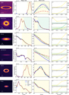 |
Fig. D.4 Same as Fig. D.2. |
| In the text | |
Current usage metrics show cumulative count of Article Views (full-text article views including HTML views, PDF and ePub downloads, according to the available data) and Abstracts Views on Vision4Press platform.
Data correspond to usage on the plateform after 2015. The current usage metrics is available 48-96 hours after online publication and is updated daily on week days.
Initial download of the metrics may take a while.