| Issue |
A&A
Volume 695, March 2025
ZTF SN Ia DR2
|
|
|---|---|---|
| Article Number | A264 | |
| Number of page(s) | 22 | |
| Section | Stellar structure and evolution | |
| DOI | https://doi.org/10.1051/0004-6361/202449746 | |
| Published online | 25 March 2025 | |
ZTF SN Ia DR2: High-velocity components in the Si IIλ6355
1
School of Physics, Trinity College Dublin, College Green, Dublin 2, Ireland
2
Oskar Klein Centre, Department of Astronomy, Stockholm University, SE-10691 Stockholm, Sweden
3
Oskar Klein Centre, Department of Physics, Stockholm University, SE-10691 Stockholm, Sweden
4
Institute of Physics, Humbolt-Universität zu Berlin, Newtonstr. 15, D-12489 Berlin, Germany
5
Univ Lyon, Univ Claude Bernard Lyon 1, CNRS, IP2I Lyon/IN2P3, UMR 5822, F-69622 Villeurbanne, France
6
Department of Physics, Lancaster University, Lancs LA1 4YB, UK
7
Université Clermont Auvergne, CNRS/IN2P3, LPCA, F-63000 Clermont-Ferrand, France
8
Instituto de Estudios Astrofísicos, Facultad de Ingeniería y Ciencias, Universidad Diego Portales, Av. Ejército Libertador 441, Santiago, Chile
9
Department of Particle Physics and Astrophysics, Weizmann Institute of Science, Rehovot 7610001, Israel
10
Institute of Astronomy and Kavli Institute for Cosmology, University of Cambridge, Madingley Road, Cambridge CB3 0HA, UK
11
Institute of Space Sciences (ICE, CSIC), Campus UAB, Carrer de Can Magrans, s/n, E-08193 Barcelona, Spain
12
Institut d’Estudis Espacials de Catalunya (IEEC), E-08034 Barcelona, Spain
13
Department of Physics and Astronomy, Northwestern University, 2145 Sheridan Road, Evanston, IL 60208, USA
14
Center for Interdisciplinary Exploration and Research in Astrophysics (CIERA), 1800 Sherman Ave., Evanston, IL 60201, USA
15
Nordic Optical Telescope, Rambla José Ana Fernández Pérez 7, ES-38711 Breña Baja, Spain
16
INAF – Osservatorio Astronomico di Padova, Vicolo dell’Osservatorio 5, I-35122 Padova, Italy
17
Division of Physics, Mathematics, and Astronomy, California Institute of Technology, Pasadena, CA 91125, USA
18
IPAC, California Institute of Technology, 1200 E. California Blvd, Pasadena, CA 91125, USA
19
Caltech Optical Observatories, California Institute of Technology, Pasadena, CA 91125, USA
⋆ Corresponding author; This email address is being protected from spambots. You need JavaScript enabled to view it.
Received:
26
February
2024
Accepted:
6
February
2025
Abstract
The Zwicky Transient Facility SN Ia Data Release 2 provides a perfect opportunity to perform a thorough search for and subsequent analysis of Si IIλ6355 high-velocity features (HVFs) in the pre-peak regime. The source of such features remains unclear, but potential origins include circumstellar material, as well as enhancements to the abundances or densities intrinsic to the supernova (SN) ejecta. Therefore, they may provide clues to the elusive progenitor and explosion scenarios of Type Ia SNe (SNe Ia). We employed a Markov chain Monte Carlo fitting method followed by Bayesian information criterion testing to classify single and double Si IIλ6355 components in the DR2. The detection efficiency of our classification method was investigated through the fitting of simulated features, which allowed us to place cuts on the spectral quality required for reliable classification. These simulations were also used to perform an analysis of the recovered parameter uncertainties and potential biases in the measurements. Within the 329 spectra sample we investigated, we identified 85 spectra exhibiting Si IIλ6355 HVFs. We find that HVFs decrease in strength with phase relative to their photospheric counterparts; however, this decrease can occur at different phases for different objects. HVFs with larger velocity separations from the photosphere were observed to fade earlier, leaving only the double components with smaller separations as we moved towards maximum light. Our findings suggest that around three quarters of SN Ia spectra before −11 d show high-velocity components in the Si IIλ6355, with this dropping to around one third in the six days before maximum light. We observed no difference between the populations of SNe Ia that do and do not form Si IIλ6355 HVFs in terms of the SALT2 light curve parameter x1, peak magnitude, decline rate, host mass, or host colour, supporting the idea that these features are ubiquitous across the SN Ia population.
Key words: techniques: spectroscopic / supernovae: general
© The Authors 2025
 Open Access article, published by EDP Sciences, under the terms of the Creative Commons Attribution License (https://creativecommons.org/licenses/by/4.0), which permits unrestricted use, distribution, and reproduction in any medium, provided the original work is properly cited.
This article is published in open access under the Subscribe to Open model. This email address is being protected from spambots. You need JavaScript enabled to view it. to support open access publication.
1. Introduction
Believed to be the thermonuclear explosion of a white dwarf due to interactions with a binary companion, Type Ia supernovae (SNe Ia) are a well-studied class of transients. With the normal SNe Ia following a strict relationship between their absolute magnitude and their light curve shape (Pskovskii 1977; Phillips 1993), their application as standardised candles was key to the discovery of the accelerating expansion of the Universe and, in turn, dark energy (Riess et al. 1998; Perlmutter et al. 1999).
The observational properties and evolution of SNe Ia have been well investigated in the literature, leading to further subdivision of the class into an ever-growing number of subclasses (see Taubenberger 2017, for a review). Many diagnostics have been developed to explore this diversity, grouping together clusters of similar SNe Ia in various parameter spaces, many of which revolve around the Si IIλ6355 absorption feature. The Branch classification scheme (Branch et al. 2006, 2009) divides the SN Ia population into four classes (core-normal, shallow-silicon, broad-line, and cool) based on the pseudo-equivalent widths of the Si IIλ6355 and λ5972 lines at maximum light, with the shallow-silicon and cool groups broadly aligning with the 91T- and 91bg-like subtypes, respectively. Wang et al. (2009) also drew their classifications from maximum-light spectra, defining all objects with an Si IIλ6355 velocity below 12 000 km s−1 as normal-velocity SNe and those above this threshold as high-velocity SNe. Analysing not just the Si IIλ6355 velocity from a single epoch but also the rate at which this velocity drops, Benetti et al. (2005) divided the population into low-velocity gradient (LVG) and high-velocity gradient (HVG), with the post peak velocity decline as less than or greater than 70 km s−1 day−1, respectively.
While the velocities and widths of the Si IIλ6355 line have been well characterised, little focus has been given to the potential presence of high-velocity features (HVFs). Seen predominantly in the Ca II near-infrared (NIR) and Ca II H&K absorption lines in spectra taken up to maximum light (Hatano et al. 1999; Kasen et al. 2003; Wang et al. 2003; Gerardy et al. 2004; Thomas et al. 2004; Mazzali et al. 2005a,b; Maguire et al. 2014; Marion et al. 2013), these features appear as secondary absorption components several thousands of kilometres per second to the blue of the photospheric-velocity (PV) component. While less common than in the calcium, a number of SNe Ia have been seen to possess these high-velocity (HV) components in the Si IIλ6355 (Quimby et al. 2006; Childress et al. 2013; Marion et al. 2013), with HVFs also having been reported in Si III, S II, and Fe II lines (Hatano et al. 1999; Marion et al. 2013). The source of these HVFs remains uncertain, with potential origins being in density or abundance enhancements in the ejecta or their formation being due to circumstellar material (CSM; e.g. Mazzali et al. 2005a; Tanaka et al. 2006).
Few samples of HVF spectra have been constructed and studied in the past, with any discussion of HVFs typically being conducted on an object-by-object basis. Childress et al. (2014) studied a sample of 58 low-redshift (z ≤ 0.03) SNe Ia with maximum light spectra in order to investigate the relation between the Si IIλ6355 and Ca II NIR features. Their analysis of the strengths of the HV components in the Ca II NIR feature indicated that HVF strength decreases with increasing light curve decline rate, and it is absent altogether in the rapidly evolving targets. Ca II NIR HVF strength was also shown to decrease with increasing silicon velocity at maximum light, with Ca II NIR HVFs being absent in high velocity SNe Ia (vSi ≥ 12 000 km s−1 at peak; Wang et al. 2009). Maguire et al. (2014) investigated a sample of 264 SNe Ia from the Palomar Transient Factory (PTF), which included spectra obtained more than two weeks before maximum light. They found that HVFs in the Ca II NIR line appear to be ubiquitous at early times, with ∼95% of SNe Ia with a spectrum before –5 days from peak displaying an HV component.
Silverman et al. (2015) conducted a search for HVFs in 445 spectra from 210 objects in the Si IIλ6355, Ca II NIR, and H&K features. Their results agreed with Childress et al. (2014) in finding under-luminous objects to lack Ca II NIR HVFs, unlike the rest of the subclass. The less common Si IIλ6355 HVFs were shown to only appear at earlier phases and are more commonly found accompanied by higher photospheric velocities. Silverman et al. (2015) also found stronger HV components in the Si IIλ6355 in objects lacking early C II absorption, with redder colours around the peak.
This work aims to identify spectra in the Zwicky Transient Facility (ZTF; Bellm et al. 2019; Graham et al. 2019; Masci et al. 2019; Dekany et al. 2020) Cosmology Data Release 2 (ZTF Cosmo DR2 or simply DR2; Rigault et al. 2025) possessing HV components in the Si IIλ6355 feature and then analyse the resulting distributions of phase, component velocity separation (Δv), and corresponding light curve properties as well as to investigate the correlations drawn from previous samples. In Sect. 2, we introduce the dataset. In Sect. 3, we present the fitting algorithm for the spectra and our simulations. The results of the fitting to the real data are presented in Sect. 4 and subsequently discussed in the context of the literature in Sect. 5.
2. Observations and sample definition
The ZTF Cosmo DR2 comprises the ZTF data for SNe Ia in the first three years of operations (2018–2020), which is the largest SN Ia sample to date from a single untargeted survey. This dataset consists of forced photometry light curves and spectroscopy for each SN Ia. A dataset overview containing statistics and technical details concerning the photometric and spectroscopic observations, as well as details on sub-classifications and host associations, can be found in Rigault et al. (2025), along with a list of accompanying analysis papers written by the ZTF Ia working group.
2.1. Data acquisition and reduction
The SN Ia spectra in our sample came from a variety of sources. In this section we describe the instruments and telescopes, as well as the data reduction technique for each telescope and instrument setup. Our measurements were sensitive to the wavelength and relative flux calibration across the Si IIλ6355 feature, but we did not make use of the absolute values so absolute flux calibration to photometric measurements was not performed. These spectra are being publicly released as part of the ZTF DR2 data release, with details on how to access the spectra and metadata provided in Rigault et al. (2025). We performed a number of cuts on our sample to select pre-maximum light spectra that had reliable phase estimates from their light curves and had sufficient signal-to-noise (S/N) in the region of the Si IIλ6355 feature (see Sect. 2.2).
Spectra from the European Southern Observatory’s (ESO) New Technology Telescope (NTT) were obtained with ESO Faint Object Spectrograph and Camera version 2 (EFOSC2; Buzzoni et al. 1984) as part of the ePESSTO and ePESSTO+ collaborations (Smartt et al. 2015) at the La Silla Observatory. These spectra were reduced using a custom built pipeline described in Smartt et al. (2015) to provide wavelength- and flux-calibrated spectra. A number of spectra come from the 2 m Liverpool Telescope (LT; Steele et al. 2004) using the Spectrograph for the Rapid Acquisition of Transients (SPRAT; Piascik et al. 2014) at the Observatorio del Roque de los Muchachos. The spectra were reduced with the pipeline of Barnsley et al. (2012), adapted for SPRAT, along with a custom Python pipeline (Prentice et al. 2018).
Spectra were obtained with the SuperNova Integral Field Spectrograph (SNIFS; Aldering et al. 2002) on the University of Hawai’i 88-inch Telescope (UH88) at the Mauna Kea Observatories. The spectra were reduced using the pipeline of the Spectroscopic Classification of Astronomical Transients (SCAT) Survey (Tucker et al. 2022). This pipeline is insufficient for studies involving absolute spectrophotometric calibration. However, our measurements involve velocities and relative line fluxes of the Si IIλ6355 feature and so this is not an issue. We are also not concerned with the region affected by the dichroic crossover (∼5000–5200 Å) that require special flat field images that are not applied by this pipeline. Spectra were also obtained at the Las Cumbres Observatory’s FLOYDS Spectrograph on the Faulkes Telescope North (FTN) and on the Faulkes Telescope South (FTS) at Haleakala and Siding Spring, respectively (Brown et al. 2013). These spectra were reduced and calibrated using a custom pipeline1 described in Valenti et al. (2014).
The KAST Spectrograph (Miller & Stone 1993) on the Shane 3 m Telescope at the Lick Observatory was used to obtain spectra that were reduced and calibrated using a custom Python pipeline, as detailed in Dimitriadis et al. (2022). Spectra were obtained with the Low Resolution Imaging Spectrometer (LRIS; Oke et al. 1995; McCarthy et al. 1998; Rockosi et al. 2010) on the Keck I telescope and reduced and calibrated using LPIPE (Perley 2019). The spectrum obtained with the Deep Imaging Multi-Object Spectrograph (DEIMOS) on the Keck II telescope was reduced using the PYPEIT software package (Prochaska et al. 2020)2. The Double Beam Spectrograph (DBSP) on the 200-inch Telescope (P200) at Palomar Observatory was used to obtain a number of spectra, these were reduced used a PyRAF-based pipeline, ‘pyraf-dbsp’ (Bellm & Sesar 2016).
Spectra were obtained with the Asiago Faint Objects Spectrograph and Camera (AFOSC) on the 1.82 m Copernico Telescope at the INAF Osservatorio Astronomico di Padova. They were reduced using standard tasks in IRAF, including wavelength calibration with arc lamp spectra and flux calibration using spectrophotometric standard stars. The spectra obtained at Alhambra Faint Object Spectrograph and Camera (ALFOSC) on the Nordic Optical Telescope (NOT) at the Observatorio del Roque de los Muchachos was reduced using a custom PYPEIT (Prochaska et al. 2020) environment3. Spectra were obtained using the Dual Imaging Spectrograph (DIS) on the Astrophysical Research Consortium 3.5 m Telescope (ARC) at the Apache Point Observatory (APO) and reduced using standard routines in IRAF, as in e.g. Sharma et al. (2023). Spectra obtained at the Goodman Spectrograph (Clemens et al. 2004) on the Southern Astrophysical Research Telescope (SOAR) at Cerro Tololo Inter-American Observatory were reduced and calibrated using a custom Python pipeline, as detailed in e.g. Dimitriadis et al. (2022). Spectra were obtained with the Focal Reducer and Low Dispersion Spectrograph 2 (FORS2) on UT1 of the Very Large Telescope (VLT) at the ESO Paranal Observatory. These spectra were reduced using a custom Python pipeline4 based on PYPEIT (Prochaska et al. 2020).
Spectra were observed with the Inamori-Magellan Areal Camera and Spectrograph (IMACS Dressler et al. 2011) mounted on the Magellan-Baade telescope at Las Campanas observatory. The data reduction was performed in IRAF5 following standard reduction procedures. The Low Dispersion Survey Spectrograph 3 (LDSS-3; Stevenson et al. 2016) on the Magellan-Clay Telescope at Las Campanas Observatory was used to obtain one spectrum, which was reduced using standard IRAF routines as described in Hamuy et al. (2006) using the same procedure as described for IMACS above.
Spectra were obtained with the Optical System for Imaging and low-Intermediate Resolution Integrated Spectroscopy (OSIRIS; Cepa et al. 2000) on the Gran Telescopio Canarias (GTC) at the Observatorio del Roque de los Muchachos. These data were reduced and calibrated following the method in Piscarrera et al. (in prep.) using custom routines based on PYPEIT (Prochaska et al. 2020). Some spectra were obtained with the Device Optimized for the Low Resolution (DOLORES) on the Telescopio Nazionale Galileo (TNG) at the Observatorio del Roque de los Muchachos and reduced using PYPEIT (Prochaska et al. 2020), following Das et al. (2023).
Spectra were obtained with Gemini Multi-Object Spectrographs (GMOS; Hook et al. 2004; Allington-Smith et al. 2002) on the Gemini North Telescope at the Mauna Kea Observatories. The spectra were reduced using standard IRAF and PYRAF and Python routines, following Dimitriadis et al. (2022). The Intermediate-Dispersion Spectrograph and Imaging System (ISIS) and the Auxiliary-port Camera (ACAM; Benn et al. 2008) on the William Herschel Telescope (WHT) at the Observatorio del Roque de los Muchachos were used to obtain spectra. These were reduced and calibrated using standard IRAF routines. The Robert Stobie Spectrograph (RSS; Kobulnicky et al. 2003) on the South African Large Telescope (SALT; Buckley et al. 2006) at the South African Astronomical Observatory (SAAO) was used to obtain spectra. The spectra were reduced using the custom pipeline, PySALT (Crawford et al. 2010) to produce wavelength- and flux-calibrated spectra. Spectra were obtained with the DeVeny spectrograph on the 4.3 m Discovery Channel Telescope (DCT), which was reduced using standard IRAF routines, including wavelength and flux calibration (Hung et al. 2017). The Spectral Energy Distribution Machine (SEDm; Blagorodnova et al. 2018; Kim et al. 2022; Lezmy et al. 2022) on the P60 (Cenko et al. 2006) was used to obtain spectra, which were subsequently reduced using PYSEDM (Rigault et al. 2019).
We did not require absolute flux calibration for our measurements but our measurements were impacted by the relative flux and the wavelength calibration. Not all the spectral reduction techniques used for our sample provide meaningful flux uncertainties. Therefore, as described in Sect. 3.1.1, we estimated the uncertainty on the flux using the standard deviation of the values in certain continuum regions near to the feature of interest. For SN Ia spectra, where flux uncertainties were available, we cross-checked against the uncertainty estimates from the standard deviation near the feature of interest and found them to be consistent. In Sect. 2.2 we describe how we performed a cut on the sample based on the S/N in the Si IIλ6355 region. Each remaining spectrum after this cut was inspected manually while choosing the continuum regions and if any cosmic rays or host galaxy lines were identified they were masked out prior to fitting the Si IIλ6355 feature. We include an uncertainty in our fitting of 200 km s−1 to account for additional velocity offsets associated with motions of the SNe Ia in their host galaxies.
2.2. Sample definition
The starting point for defining our sample was the subset of the 3628 confirmed SNe Ia in the DR2 with spectra from the aforementioned facilities for which sufficient data information and reliable reductions could be performed, amounting to 3585 targets with 5028 spectra. 43 SNe Ia that were included in the full DR2 data release were excluded from our sample due to a lack of sufficient information on the observations and data reduction techniques. As our analysis was to be restricted to spectra in the pre-peak regime, we required sufficient photometry to produce a reliable estimate of spectral phase. We used the suggested cuts of Rigault et al. (2025) on the SALT2 light curve fitter (Guy et al. 2007) outputs, of fit probability greater than 10−5 and uncertainties smaller than the quoted values for the light curve width parameter, x1 (δx1 < 1), colour parameter, c (δc < 0.1), and the time of maximum light, t0 (δt0 < 1 d). We did not impose any constraints on the measured values of x1 or c.
To maximise our spectral sample, we investigated all SNe Ia that failed to meet these criteria in order to avoid cutting otherwise acceptable spectra solely due to poor phase estimates from sparse photometry. In many cases this involved fitting supplementary photometry obtained from other surveys. A summary of this investigation and the updated phase estimates can be found in Appendix A. Following this investigation we were left with 4572 spectra for which we had reliable phase estimates. As we were specifically interested in the evolution of Si IIλ6355 HV components, we limited our search to the pre-peak regime when these features are expected to be present. Cutting any spectra with a phase post-peak, we were left with 2362 spectra from 1801 SNe Ia.
To assess the spectral quality in the vicinity of the Si IIλ6355 we defined a local S/N as the ratio of the depth of the Si IIλ6355 to the standard deviation in the regions of the continuum to the red and blue (continuum region selection is discussed in detail in Sect. 3.1). This measurement was made once the continuum had been removed and was repeated 1000 times with different continuum selection points. The final S/N estimate was taken as the mean of these 1000 values. In making these estimates we identified 432 spectra that either did not cover the wavelength range of the Si IIλ6355 feature, or did not have a clearly visible Si IIλ6355 feature from which to compute an estimate of local S/N. These spectra were cut from the sample and the measurements of S/N for the remaining objects are presented in Fig. 1, along with the distribution of dispersion (average separation between pixels in Å) and the redshift distribution of the corresponding SNe. The large peak at ∼25 Å in the spectral dispersion panel corresponds to the spectra coming from the Spectral Energy Distribution Machine (SEDM; Blagorodnova et al. 2018; Rigault et al. 2019) on the P60 (Cenko et al. 2006) at the Palomar Observatory. The SEDM provides ∼60% of the full DR2 spectral sample. The usefulness of the SEDM spectra in the search for HVFs is determined by the simulations in Sect. 3.2, where we place a cut on both dispersion and S/N.
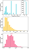 |
Fig. 1. Distributions of resolution and S/N in the 1930 spectra before the peak covering the relevant wavelength region with a clean enough signal for the S/N estimation. The bottom panel represents the redshift distribution of the 1557 objects sampled by these spectra. The dotted lines and accompanying values correspond to the medians of the three measurements. Final cuts upon S/N and resolution will be implemented based upon the results of the simulated fits. |
3. Method
In Sect. 3.1 we detail the procedure for fitting the Si IIλ6355 and our method of classifying HVFs and non-HVFs. In Sect. 3.2 we describe the formulation of our synthetic Si IIλ6355 features, as well as present the simulation results that test the ability of our method to identify HVFs. Based on these results, we can determine the dispersion and S/N that are required to identify HV components in observed spectra. We also investigate the simulation results to assess potential biases in our measurements of the feature parameters.
3.1. Identification of high-velocity components in the Si IIλ6355
Our aim is to distinguish between those SN Ia spectra that possess an HV component in the Si IIλ6355 line and those that do not. The feature fitting with single and double component models is performed with an Markov chain Monte Carlo (MCMC) framework using the EMCEE package (Foreman-Mackey et al. 2013), treating the local continuum as linear and leaving the corresponding slope and intercept as free parameters in the fitting.
3.1.1. Spectral line fitting
As for the S/N estimation discussed in Sect. 2.2, the line fitting requires defined continuum regions to the blue and to the red of the Si IIλ6355 absorption feature. The so-called ‘continuum’ in these photospheric phase spectra is in fact the overlapping of many different P-Cygni emission profiles and as such we are actually defining a pseudo-continuum. This pseudo-continuum region selection is more complex for the observed data than for the simulated features for reasons such as contamination by neighbouring features and noise spikes. The initial selections of these local pseudo-continuum regions were performed using a gradient method similar to previous studies (e.g. Blondin et al. 2011; Nordin et al. 2011; Silverman et al. 2012, 2015). Starting at the local minimum of the feature, gradients were calculated in wavelength bins successively moving outwards to the red and blue until the gradient changed sign, indicating a maximum. The wavelength bins corresponding to these sign changes were therefore taken as the selections of the initial pseudo-continuum regions. Each selection was subsequently checked manually, and any necessary updates to the regions were made.
For each spectrum, we commenced with a pre-processing step that involves the cutting of two small regions of the spectrum (6275–6307 Å and 6860–6890 Å) corresponding to telluric regions, as well as correcting for the host galaxy redshift. We then performed a normalisation step by dividing the flux of the spectrum by the maximum value found between 200 Å to the blue of the blue continuum region and 200 Å to the red of the red continuum region. This ensured that the slopes and offsets of all the features in the fitting were of a similar order of magnitude.
The Si IIλ6355 feature is a doublet comprised of two lines very close together in wavelength space at 6347.11 and 6371.37 Å. Our feature fitting assumes the two singlets of the Si IIλ6355 doublet to be tied in all parameters (velocity, depth, and width) as is the case under the assumption of an optically thick regime at these pre-peak phases (see discussion in Childress et al. 2013). The single component model corresponds to one Si IIλ6355 doublet, typically associated with the photosphere, and therefore, we call this the PV component. The double-component model includes an additional Si IIλ6355 doublet at higher velocity, which we refer to as the HV component.
The single (f1) and double (f2) component models take the forms
 (1)
(1)
and
 (2)
(2)
with f as the flux; s and i as the continuum slope and intercept, respectively; and g(λ, a, b, c) being an indivdual Si IIλ6355 doublet of the form
 (3)
(3)
where a is the depth of one of the singlets; b is the wavelength position of the minimum, with the 7.89 and 16.37 quantities as the offsets from 6355 Å for the 6347.11 Å and 6371.37 Å lines of the doublet; c is the width; and the PV and HV subscripts refer to the PV and HV components of the model, respectively. The uncertainty on the flux values is taken as the standard deviation of the points in the continuum regions around the linear fit used for the initialisation of s and i.
We placed a number of priors on the MCMC fitting to restrict the walkers to the relevant region of the parameter space. The depth parameters (aPV and aHV) and width parameters (cPV and cHV) were bound to be larger than 0.05 and 30 Å, respectively to avoid overfitting, especially in the noisier and lower resolution spectra. To ensure that the fitted components fall within the wavelength region of the feature we introduced the restrictions that the sum bPV + cPV was smaller than the lower bound of the red continuum region and than bHV − cHV was higher than the upper bound of the blue continuum region (or bPV − cPV in the single component model).
Through preliminary testing with simulated features (see Sect. 3.2.1), we found that in most cases the slope from a linear fit to the continuum regions provided a smaller residual with the true value than that of the final output of the MCMC. This effect was counteracted by placing a uniform prior on the slope parameter, with dispersion-dependent limits d away from this slope estimate derived empirically as
 (4)
(4)
with r as the dispersion in Å/pix.
The measured values for the parameters were taken as the medians of the posteriors, with the lower and upper uncertainties as the 16th and 84th percentiles, corresponding to a 68% confidence interval. We used the MCMC chains to calculate parameters such as pseudo-equivalent widths (pEWs), pEW ratios, and velocity separations directly, drawing the median and lower and upper uncertainties from the resulting posteriors. The accuracy of these uncertainties is investigated with the simulated data in Sect. 3.2.
3.1.2. Deciding upon the preferred model
With single- and double-component posterior distributions derived from the MCMC, we employed the Bayesian information criterion (BIC) – a goodness-of-fit metric that disfavours more complex models – to decide upon the preferred model. As there are three more free parameters in the double-component model than the single-component model, the corresponding fit has to significantly improve the goodness-of-fit in order to be preferred by the BIC. We employed the BIC as
 (5)
(5)
with L as the maximised value of the likelihood function, k as the number of free parameters (five for the single and eight for the double component), and N as the number of data points in the fitting. The model that produces the lowest BIC was provisionally deemed to be the best match, subject to two cuts explained below.
The HV components that possess large velocity separations from their PV counterparts are easily distinguishable through fitting or visual inspection. However, as this velocity separation decreases, the components become increasingly more entangled and more difficult to detect. With the addition of noise, this has the potential to lead to high false-positive rates. Therefore, a cut upon the minimum velocity separation was necessary in the fitting, as below this limit we were not be able to reliably differentiate between single and double component features. A lower limit of 4500 km s−1 was adopted in Silverman et al. (2015). Our lower limit of 4000 km s−1 was set based on the performance of our classification method on simulated data (Sect. 3.2). Similarly to Silverman et al. (2015), we considered any two-component classifications with a PVF velocity ≤ 9000 km s−1 as unreliable, with the fitted PV component likely corresponding to contaminating C II absorption. Therefore, in these cases we chose the single- over double-component classification, regardless of the BIC-based classification.
3.2. Simulations
To investigate the accuracy of the MCMC/BIC method described in Sect. 3.1 for identifying HV components, as well as its ability to recover the injected parameters, we generated synthetic Si IIλ6355 features. The results from these simulations were also used to inform cuts on dispersion and S/N in the observed data. In Sect. 3.2.1 we describe the construction of our simulated data for testing our method, while in Sect. 3.2.2 we detail our detection efficiencies and in Sect. 3.2.3, we discuss the correction for biases in our fitting based on our simulations.
3.2.1. Constructing the simulated data
The synthetic features were comprised of two (PV and HV) doublet components, separated by a fixed velocity difference – with the exception of the simulations where we injected no HV component to assess the false-positive rate. We created a grid spanning four S/Ns (4, 8, 15, and 25), four dispersions (2, 5, 10, and 25 Å/pix) to cover the range of values found for the DR2 subsample (Fig. 1), as well as seven velocity separations (no HVF, 3000, 4000, 5000, 6000, 7000, and 8000 km s−1) covering the range of separations expected from the data. For each of these parameter setups we generated 500 simulated features.
Measurements from PTF SNe Ia (Maguire et al. 2014) were used to inform our generation of Si IIλ6355 line profiles. For each feature, we generated a random phase between –17 and 0 d, which then gave a probability distribution of photospheric velocities as the cross-section of the power-law fit to the PTF data seen in the top panel of Fig. 2. We drew a photospheric velocity from this resulting distribution, with the HVF velocity then defined by the fixed velocity separation in the simulation. The depths and widths of both components were drawn from a kernel density estimate (KDE) of the PTF measurements found in the bottom panel of Fig. 2. The modelling of the HV components in these simulations was rather simplistic, with the depths and widths assumed to follow the same distribution as those of the PV components. The photospheric velocity, width, and depth estimates based on Maguire et al. (2014) were also biased since these include contributions from HVFs. The validity and potential implications of these assumptions can be assessed with our final DR2 sample and are discussed in Sect. 4.2.
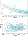 |
Fig. 2. Palomar Transient Factory (Maguire et al. 2014) SN Ia spectral measurements for velocity, width, and depth in the case of the Si IIλ6355 absorption feature. The power law fit to the velocity evolution and the Gaussian KDE (described by the contours) for the width and depth are used to inform the generation of the synthetic features in the simulations. |
Noise was introduced to the simulated features and surrounding continuum based on the set S/N values defined by the simulation grid. Noise values for each wavelength bin were then drawn from a Gaussian distribution centred about zero with a standard deviation as the product of the S/N and the depth of the composite feature. The dispersion of each simulated feature was simply defined as the separation between the wavelength bins (the same definition as used for the observed spectra). With this simulated feature constructed, we introduced a simple linear continuum to each feature, varying the slope and intercept between them. The values for these slopes were drawn from the normal distribution with mean −1.9 × 10⁻⁴ and standard deviation 1.7 × 10⁻⁴, chosen to match the range of initial slope estimates from the normalised DR2 spectra.
Our simulated spectra with the single- and double-component models were then fit following the procedure described in Sect. 3.1. The continuum region selection for the simulated data was performed in a similar fashion to that of the observed data but did not require manual checking for cosmic ray spikes or contamination by host lines.
3.2.2. Detection efficiencies
We performed simulations of the Si IIλ6355 region with different S/Ns, dispersions, and the presence (at different velocity separations between the two components) or absence of an HV component. We present the resulting true- and false-positive rates for the detection of HVFs for each of the different simulation setups in Fig. 3. The panels display the four S/N ratios increasing from left to right, with the different colours indicating the four different dispersions. The circle markers correspond to the left axis and display the percentage of the 500 simulated features in that simulation that were correctly identified as possessing both a HV and PV component. The arrows correspond to the right axis and represent the percentage of the 500 simulated features without an HV component that were incorrectly identified as possessing two components. The uncertainties on these points are taken as binomial and calculated from the Clopper-Pearson method with a 95% confidence interval.
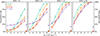 |
Fig. 3. True (circles) and false (arrows) positive rates of the MCMC/BIC classification method as a function of the velocity separations derived from the simulations for increasing S/Ns (from left to right in the panels) and different spectral dispersions (shown as different colours). One-dimensional slices (in Δv space) of the 3D GP interpolation of S/N, dispersion, and velocity separation are presented as the coloured lines and associated 68% confidence interval regions. |
Each simulation setup in our grid can be thought of as a point in a 3D parameter space spanning S/N, dispersion, and velocity separation. At every point in this space there exists some true-positive rate that can be used to assess how probable it is to correctly identify an HV component with such properties. Using the Gaussian Process (GP) module within SCIKIT-LEARN (Pedregosa et al. 2011) we performed a 3D interpolation of this discrete grid to obtain a continuous view of the changing detection efficiency. One-dimensional slices in velocity space are shown in Fig. 3.
Our aim was then to introduce cuts based on the velocity separation, S/N, and dispersion to keep the true-positive rate high and the false-positive rate to a minimum, while maximising our sample size. As one might expect, we see an increase in our ability to correctly identify HVFs as the noise is reduced, as we improve the spectral resolution (decrease the dispersion), and as we separate the components in velocity space. The highest dispersion simulations (purple in Fig. 3) have a separation of 25 Å between wavelength bins and represent the large percentage of DR2 spectra coming from the SEDm spectrograph. Accompanying the smaller true-positive rates for these features, we see large false-positive rates of the order 15–20%. These false-positive rates also stand as lower thresholds for the true-positive rates as we can see for the 25 Å/pix lines in the left hand panel, where the true-positive rates flatten off and plateau at the level of the false-positive rate as we approach smaller velocity separations. This levelling off of the true-positive rate as it becomes similar in magnitude to the false-positive rate causes an overlap effect between the 25 Å/pix simulations and those with smaller dispersions. The simulations with S/N of four exhibit the same overlap effect as seen for the 25 Å/pix dispersion simulations for the 10 Å/pix dispersion spectra for velocity separations up to 5000 km s−1.
Due to these issues with the lowest resolution and lowest S/N spectra, we cut all spectra from our observed sample with a dispersion greater than 10 Å/pix and S/N < 8. With this dispersion cut, we removed all SEDm spectra from our sample, which due to its brighter limiting magnitude for targets compared to the other telescopes, may have potentially removed brighter events from the sample. We test the impact of this on our demographic comparison in Sect. 4.3 but found no bias in SALT2 x1 for our sample compared to the volume-limited DR2 sample. Our S/N cut could have also potentially biased our sample, removing events with intrinsically shallower Si IIλ6355 features. However, ‘shallow silicon’ (Branch et al. 2006) SNe Ia have light curve widths (parametrised by e.g. SALT2 x1) that are higher than mean of the SNe Ia sample (e.g. Blondin et al. 2011) and we found no x1 bias relative to our comparison DR2 sample, again suggesting that this S/N cut did not introduce a significant bias to our final sample. With these two spectral quality cuts in place, we obtained our final sample of 329 observed spectra from 307 SNe ready for fitting. The breakdown of each of the cuts can be found in Table 1.
Breakdown of the number of spectra/SNe Ia remaining after each cut to reach the final sample of 329 spectra ready for fitting.
The final result to be drawn from Fig. 3 was a cut upon the measured velocity separation based on the simulations. Silverman et al. (2015) chose to disregard any classifications of features with separations less than 4500 km s−1, instead classifying these spectra as having single components. We chose a similar threshold of 4000 km s−1, as below this velocity we begin to see the previously discussed overlap effect below 4000 km s−1 for the 10 Å/pix simulations with S/N of eight (lowest final resolution and S/N studied). This is further justified by closer inspection of the false positive rate. Averaging over all simulations passing the implemented dispersion and S/N cuts, we found a false positive rate of ∼1%, with 80% of these false positive classifications measured with velocity separations less than 4000 km s−1. Applying this velocity separation cut reduces the simulation false positive rate to ∼0.2% in the remaining simulations. Given that the simulations represent the ideal scenario with linear continua, generated Gaussian features, and Gaussian noise, this rate is optimistic; therefore, we assumed a more conservative false positive rate of 2%. The false positives as measured in the DR2 are likely to be concentrated at smaller velocity separations up to ∼5000 km s−1 where there exists more degeneracy between the single and double component models.
3.2.3. Parameter recovery and uncertainty corrections
Along with estimating the detection efficiencies of our MCMC/BIC HVF classification method, the grid of simulations also allowed us to test how the estimated uncertainties perform in terms of truly representing 68% confidence intervals, and identify potential biases in our measurements. The pull for some parameter X is calculated as
 (6)
(6)
with σX as the uncertainty taken from the posterior distribution. In the case of no biases and uncertainties that truly reflect 68% confidence intervals, these distributions should be Gaussian with a mean of zero and a standard deviation of unity.
In Fig. 4 we show example distributions of the pulls in the six parameters describing the PV and HV components, as well as the pEWs, RHVF (the ratio of pEWHV/pEWPV), and Δv from a simulation with our middle remaining dispersion of 5 Å/pix and middle remaining S/N of 15, with a velocity separation of 5000 km s−1. As clearly visible for the majority of the measured parameters, the spread of the pull distribution is too large with a mean standard deviation of ∼1.3 about the mean for this set of simulation parameters, indicating that the uncertainties from the MCMC posterior are ∼1.3 times too small. A pull is also observed in most parameters where the means of the distributions do not lie exactly at zero.
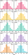 |
Fig. 4. Distribution of the pulls (residual/uncertainty) for the six feature parameters in the case of spectra with an S/N of 15, a dispersion of 5 Å/pix, and a velocity separation of 5000 km s−1. The solid black lines indicate the desired zero pull value, while the solid coloured lines indicate the means of the distributions, the values of which are shown in the top left corner of each panel. The dotted lines display the measured standard deviations. |
In Fig. 5, we present the standard deviations for each of the parameters as a function of dispersion and split into the three remaining S/N (8, 15 and 25). All two-component fits with resulting velocity separation measurements below the 4000 km s−1 threshold have already been removed. Most of the 2 Å/pix dispersion simulations exhibit standard deviations close to unity and therefore require little to no correction. The standard deviations of the pull generally increase with increasing dispersion for all S/N simulations. The thick black lines present linear regressions to these combined S/N standard deviation trends and are used to compute scale factor corrections to the uncertainties to bring them in line with 68% confidence intervals.
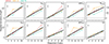 |
Fig. 5. Standard deviations of the pull distributions about their means for each of the simulations. The three S/Ns are represented by different colours, as indicated above the top-left panel. The thick solid lines describe the linear regression fits to the data points with each of the three dispersions. The black point in each panel presents the standard deviation of the points around this fit. We highlight that the RHVF panel has a different y-axis scaling due to the larger standard deviation values. |
In a similar fashion, we can analyse how closely the means of these pull distributions lie to zero to identify any biases in the measurements. In Fig. 6 we plot the means of the pull distributions for each of the simulations as a function of dispersion, after having applied the uncertainty corrections discussed above. We observe slight biases that are consistent between the different S/N and dispersion pairings and appear relatively flat with changing dispersion. We correct for these trends using a linear regression as a function of dispersion. The same investigation was performed for the single component fits to the simulated features with no HV components. While we find the means to be centred upon zero – indicating no bias in the measurements – the standard deviations of these distributions fell in the range 1–1.3, and therefore, small corrections were made to the uncertainties using the same method as for the two-component fits above.
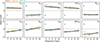 |
Fig. 6. Means of the pull distributions for each of the simulations after applying the uncertainty corrections. The formatting matches that of Fig 5. The thick black lines present linear regressions to these trends that can be used to characterise and then correct for the biases. The black point in each panel presents the standard deviation of the points around this fit. |
4. Results
With the cuts informed by the simulations (dispersion ≤ 10 Å/pix and S/N ≥ 8), we obtained our final sample of 329 spectra (see Table 1) for which we studied the presence of HVFs in the Si IIλ6355. With the MCMC/BIC classification method outlined in Sect. 3.1, we fit our sample, taking all those classified as HVF with vPV > 9000 km s−1 and Δv > 4000 km s−1 as our HVF subsample. Of the 329 spectra we identified 85 as possessing both PV and HV components, corresponding to 26% of the sample. The HVF spectral sample comprises spectra from 75 SNe, including eight objects for which we found these HV components in multiple epochs. In the sample, there exists one object (ZTF18abauprj) for which we have both HVF spectra and a final epoch showing no sign of an HV component, providing a glimpse at the full evolution of these features as time evolves. In our sample, we also have ten pairs of spectra from the same object coming from different instruments with phase separations of a day or less. In all these cases the classifications were consistent between these spectra with six pairs as PVF and four as HVF. The measured values for velocity for all these components were consistent within the uncertainties, as were the feature widths and the majority of the feature depths. Any differences in the depth parameters – which are all ≤0.05 in size – were likely predominantly the result of changing line profiles over the hours elapsed between the spectra, although there may be small systematic differences.
In Sect. 4.1 we describe how the observed SN measurements were used to validate the priors used in the simulations. In Sect. 4.2 we explore the phase evolution of the HVFs. We then define and analyse a reduced low-bias sample to draw conclusions about the properties of HVFs in Sect. 4.3, and correlations with light curve and host parameters in Sect. 4.5.
4.1. Validation of simulation priors
The top panel of Fig. 7 displays the measured velocity evolution for the 329 spectra from our 307 SNe Ia, split into the photospheric components, and high-velocity components where classified. Power-law fits were performed to the velocities as a function of phase for the HV components, as well as three samples of the PV velocities, (i) all the PV components, (ii) just the PV components with HV counterparts, and (iii) just the singular PV components. These three fits are consistent from around –10 d onwards, with the PV velocities in objects possessing HV components drifting to higher velocities at early phases. This agrees with the findings of Silverman et al. (2015) in that HVFs tend to be accompanied by higher velocity PVFs. We also plot in grey the velocity evolution from the PTF sample (Maguire et al. 2014) that was used as reference for our Si IIλ6355 feature generation in the simulations. These PTF measurements were performed on the overall Si IIλ6355 features without distinction between PV and HV components. The PTF velocity evolution therefore likely has some level of contamination from HVFs, and would be expected to lie somewhere between our measured PVF (blue) and HVF (pink) evolution curves, as it does.
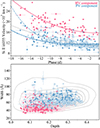 |
Fig. 7. Evolution of the velocities of the PV and HV Si IIλ6355 components for all 329 spectra in the sample (top panel). The hollow points correspond to the 244 PV components with no HV counterpart. The solid blue line is fit to all the PV components, with the dash-dotted and dotted blue lines showing fits to the PV components of spectra with and without HV components, respectively. The pink line is the fit to the HV components and the grey line is the evolution from the PTF sample (Maguire et al. 2014). The width against depth for the measured PV and HV Si IIλ6355 components using the same colours as the top panel (bottom panel). The grey contours show the KDE for the PTF sample for comparison. |
In the bottom panel of Fig. 7 we present the measured depths and widths of the singlet lines making up the PV and HV components. As for the velocity evolution we plot the comparison PTF data as grey contours to show how our final measurements align with the distributions chosen to inform the feature generation in the simulations. As expected, the distribution of PVF measurements lie in the same parameter space as the PTF data, but our measurements are slightly more compact in both dimensions, which (as with the velocity) is likely due to HVF contamination in the PTF dataset inflating the depths and widths in some cases. For the generation of the HVF components in the simulations, we made the assumption that the widths and depths of the HV components followed the same distribution. However, as clearly visible in Fig. 7, these components tend to cluster more towards shallower depths and narrower widths. While some false positive classifications may be contaminating the HVF cluster, there remains a clear distinction between the HVF and PVF distributions. To evaluate the effect that this discrepancy has upon the calculated detection efficiencies we recalculated the true-positive rates from the simulations, excluding any simulated spectra from the calculations with aHV > 0.25 or cHV > 70 Å so as to be more in agreement with the measurements from the observations. The residuals between the true positive rates these updated simulations and the original simulations are presented in Fig. 8. In most cases, the true-positive rate increases with the cut to only focus on the observed region of the parameter space. This implies that we are less sensitive to finding HV components with similar widths and depths to their PV counterparts – likely due to increased degeneracy in the fit. Therefore, we updated the detection efficiencies with a GP interpolation (following the method of Sect. 3.2.2) to these new values.
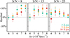 |
Fig. 8. Residuals between the true positive rates taken from simulated spectra with aHV ≤ 0.25 or cHV ≤ 70 Å and the original true positive rates as a function of velocity separation for the three S/Ns. |
4.2. Phase evolution
The evolution of the ratio of pEWHV/pEWPV (RHVF) is seen for our observed sample in the middle panel of Fig. 9. In general, the uncertainties on the measured RHVF values are large as many of the two-component fits exhibit high levels of degeneracy and posteriors of the numerator and denominator in the ratio (pEWHV and pEWPV) are inversely correlated.
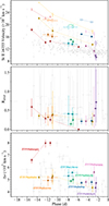 |
Fig. 9. Evolution of the component velocities (top), parameter RHVF (pEWHV/pEWPV; middle), and the separation of the PV and HV features in velocity space (bottom). The measurements for individual spectra are plotted in grey, with the coloured points and lines corresponding to SNe Ia for which we have multiple spectra. The hollow points in the top panel correspond to the HV components. The cluster of points in the middle panel at R = 0 correspond to all the spectra identified as not having an HV component. |
The SNe with multiple spectra allowed us to probe the evolution of this ratio within individual objects, with the overall sample – including single-epoch objects – giving a more global view of how the distribution of RHVF changes with phase. For most of our multi-phase objects, we possess only two spectral epochs, separated by less than ∼2.5 d, leading to very little evolution in RHVF, which appears to remain approximately constant on such small timescales. However, for ZTF19aatlmbo (SN 2019ein) and ZTF18abauprj (SN 2018cnw), we have three and four spectra spanning 9.3 d and 10.6 d, respectively. ZTF18abauprj displays a clear decrease in this ratio with time, with the HV component fading away completely somewhere between –11.4 and –5.8 d, whereas ZTF19aatlmbo exhibits a far flatter evolution; albeit with large uncertainties on the spectrum at –10.9 d. The RHVF evolution for these multi-spectra objects is consistent with previous studies showing a decline with phase, with HV components starting out strong and fading away over time (Silverman et al. 2015). As clear from these two objects, while we see a decrease in RHVF with time in individual SNe, this decay occurs at different phases, and we see many multi-spectra targets still exhibiting HVFs after the HV component in ZTF18abauprj had faded away completely. When combining the multi-spectra and single-spectra objects to get a global view of how RHVF varies with phase, we find no clear evolution, with some large and small measurements of this ratio and early and late phases, further supporting the idea that the fading away of HV components occurs at different phases in different objects.
The bottom panel of Fig. 9 presents the evolution of the velocity separation, Δv, with phase. As for RHVF, the multi-epoch spectra with small temporal differences do not shed much light upon the phase evolution of Δv. For ZTF18abauprj, we see an upwards evolution and the converse for ZTF19aatlmbo, implying that there is not a singular strict evolutionary trend for such features. However, when looking at the global evolution of the sample, we observe a dearth in the higher velocity separation spectra as we approach maximum light, with all the separations from HVF spectra after –4 d clustering below ∼5000 km s−1. This indicates more separated HV components tend to fade away at earlier phases compared to those that are more entangled with their PV counterpart.
4.3. Defining a low-bias sample
To analyse global properties of SNe Ia containing Si IIλ6355 HVFs, we were required to understand and mitigate the potential biases present in our sample that made it unrepresentative of the global SN Ia population. To this end we defined a ‘control sample’ as the 994 SNe Ia from the DR2 volume-limited (z ≤ 0.06) sample presented in Rigault et al. (2025). At this point we also removed any objects from our sample of 307 SNe that did not pass the initial suggested cuts outlined in Sect. 2.1 (fit probability > 10−5, δx1 < 1, δc < 0.1, δt0 < 1 d), reducing our ‘base sample’ to 261 SNe Ia. Through Kolmogorov-Smirnov (KS) tests between this base sample and the control sample, we can identify parameters in which our sample exhibits a significant level of bias and then eliminate these by way of a redshift-based cut. KS p-values below the threshold of 0.05 signify that the difference between the two samples is statistically unlikely to have occurred simply by chance, and points to them coming from separation populations.
The top panel of Fig. 10 presents these KS-test results for a number of measurements between the control sample and the base 261 SNe sample after imposing different redshift cuts, e.g. the data point at z = 0.04, corresponds to the KS-test between the base sample limited to SNe Ia with z ≤ 0.04 and the full control sample. The parameters investigated here are the SALT2 stretch and colours parameters, x1 and c, the phase of first photometric detection, the uncertainty in the date of maximum light (δt0), the host galaxy mass (measurements from Smith et al., in prep.), and the host galaxy redshift (not shown on plot). Our base sample of 261 SNe compared to the control sample has KS p-values that are greater than our bias threshold of 0.05 in all parameters for all redshift cut values, except c and host redshift. As we introduce more restrictive redshift cuts to our sample, we see the KS p-values for c rise, until it crosses our threshold to be considered low bias at a redshift cut of z = 0.06.
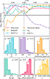 |
Fig. 10. Top: Kolmogorov-Smirnov p-values between our base sample and the control sample for six parameters. The solid black line describes the threshold below which a parameter should be considered to show a bias when compared to the ‘low-bias’ control sample. The dotted black line indicates the final redshift cut of 0.06. Bottom: Distributions of the control sample (bars) and the final sample of 190 SNe after a redshift cut at z = 0.06 (step). The p-values from the corresponding KS-tests are denoted in each of the panels. |
The comparison of the redshift distribution between the base and control samples exhibits such small p-values – for all potential redshift cuts – that it falls below the y-axis scaling of the plot in Fig. 10. This difference is not surprising at redshift cuts either far above or far below that of the control sample (z = 0.06). With a redshift cut equal to that of the control sample we see that the difference between the populations is that our sample peaks at lower redshifts, most likely due to the apparent brightness required to obtain a high enough S/N spectrum pre-peak to enter our sample. The redshift distribution describes the geometric distribution of our objects in space, with the intrinsic physics of the objects described by the other parameters. Therefore, the bias in the redshift distribution should not impact our results given that we observe no statistically significant bias in the other parameters. We consequently placed a cut at z = 0.06, leaving us with 210 spectra from 190 SNe from which to investigate global HVF properties. The distributions of these parameters in this low-bias cut sample can be seen as step plots in the bottom panels of Fig. 10 along with the control sample as the bars.
4.4. Parameter distributions
In Fig. 11 we present the distribution of velocity separations found in the 64 HVF spectra of the low-bias sample as the solid bar histogram. In general we observe a distribution skewed towards smaller velocity separations with very few spectra showing the extreme separations of 8000 km s−1. As seen in Fig. 3, our classification method is very sensitive to the larger velocity separations; however, its detection efficiency drops off as the features encroach on one another and become increasingly entangled. As an example, we have a true-positive rate of ∼25% for features with an S/N of eight and dispersion 2 Å/pix that possess a velocity separation of 4000 km s−1, implying that for every one spectrum that we identified with this parameter set, we missed three others; the true value is the number of identified targets divided by the fractional true-positive rate. Therefore, we can draw efficiency values from our 3D GP interpolation of the true-positive rates to scale the distribution of velocity separations on a spectrum-by-spectrum basis. This was first performed using the measured values of velocity separation, for which a Gaussian KDE of the probability density function (PDF) can be seen in Fig. 11 as the black solid line. To probe the potential variation of this distribution we employed a Monte Carlo method, sampling each of the velocity separations in the sample from their individual distributions – described by their measured medians and upper and lower uncertainties – before then performing the detection efficiency scaling with the resulting Δv values. This procedure was repeated 1000 times with each of these PDFs plotted as a faint orange line in Fig. 11. In each iteration we accounted for the variation due to false positives by randomly reclassifying some HVF spectra with Δv < 5000 km s−1 as non-HVF in accordance with our adopted conservative false positive rate of 2%. These final PDFs are all multiplied by the number of spectra that they represent and therefore correspond to spectrum densities instead of probabilities.
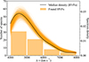 |
Fig. 11. Velocity separation distribution of the 64 HVF spectra from our low-bias sample of 210 SNe. The black curve presents the median spectrum density after correcting for the detection efficiency of our classification method. The individual orange curves correspond to 1000 iterations of sampling the Δv values from their individual measurement distributions, rescaling the distribution, and recalculating this density function. |
Figure 12 presents the phase distribution of the spectra displaying HVF against our full low-bias sample. The full sample is presented as the faint bars with the HVF spectra as the solid bars. As before, we performed the detection efficiency scaling on a spectrum-by-spectrum basis and plot the resulting density function from the velocity separation values as the solid black curve. The spectrum density function of the full phase distribution is plotted as the dotted black line. As for the velocity separation analysis, we performed Monte Carlo sampling for these two phase distributions, randomly reclassifying some HVF spectra with Δv < 5000 km s−1 as non-HVF in accordance with the false positive rate and drawing velocity separations and phases from the corresponding individual distributions to calculate new PDFs. In each of these 1000 iterations we also integrated over three phase bins to calculate the percentage of spectra exhibiting a Si IIλ6355 HV component. These three regions were divided up to each hold ∼1/3 of the 64 HVF spectra from the low-bias sample, giving bins for < –11 d, –11 to –6 d and > –6 d. The percentages of HVF spectra for these three phase ranges are shown in the bottom panel of Fig. 12 along with the shaded regions representing 68% confidence intervals calculated via the Clopper-Pearson method. These calculations indicate that we find Si IIλ6355 HV components in  % of spectra before –11 d, 46 ± 7% of spectra between –11 and –6 d, and 29 ± 5% of spectra between –6 d and maximum light. If we were to use the original detection efficiencies before introducing the cuts to only consider simulations with aHV ≤ 0.25 and cHV ≤ 70 Å (see Sect. 4.1), we calculate slightly higher percentages of
  %, 49 ± 7%, and 32 ± 5% for these three phase intervals. Therefore, Si IIλ6355 HV components are close to ∼2.5 times more common at early phases, but still appear in approximately one third of spectra in the week before maximum light.
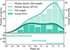 |
Fig. 12. Phase histogram for the 64 HVF spectra compared to the full 210 low-bias spectral sample. The solid black curve presents the median HVF spectrum density after correcting for the detection efficiency of our classification method, with the dotted black curve as the density of the full 210 spectra. The individual green curves (dark for HVF and pale for the full sample) correspond to 1000 iterations of sampling the Δv and phase values from their individual measurement distributions, rescaling the HVF distribution, and recalculating these density functions. |
4.5. Light curve observables and host measurements
In Fig. 13 we present the distributions of the SALT2 light curve parameter x1 for the SNe Ia in our full low-bias sample and only those showing evidence of HVFs as the faint and solid histograms, respectively. This information is then displayed in the form of SN density functions for the full sample (dotted) and those for which we have a spectrum with an identified HVF (solid). As for the Δv and phase parameters before, we performed a Monte Carlo sampling of the individual x1 measurements over 1000 iterations to assess the amount of variation in these density curves accounting for the estimated false positive rate and uncertainties in the x1 values. For each of these iterations, we integrated under the two density curves over two regions (x1 < 0 and 0≤ x1) and calculated the percentage of SNe exhibiting HV components in the Si IIλ6355. As visible in the bottom panel of Fig. 13, these two percentages (30 ± 5% and  %) are consistent with one another and support the idea of HVFs being ubiquitous across the SN Ia population. As before for the phase percentages, these uncertainties represent 68% confidence intervals.
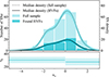 |
Fig. 13. SALT2 x1 histogram for the 56 HVF SNe compared to the full 190 low-bias sample. The solid black curve presents the median HVF SN density, and the dotted black curve indicates the density of the full 210 spectra. We performed no detection efficiency scaling upon the x1 parameter distribution. The individual blue curves (dark for HVF and pale for the full sample) correspond to 1000 iterations of sampling the x1 values from their individual measurement distributions and recalculating these density functions. |
As seen in Fig. 12, Si IIλ6355 HVFs are more prevalent at earlier phases and there is a significant decrease in the percentage of SN Ia spectra displaying HVF features as the phase approaches maximum light. By cutting the sample and repeating these percentage calculations with only the earliest phases, we can test the impact of this phase dependence on any potential trend with x1. We therefore introduced a phase cut at –8.7 d – the median HVF spectral phase – and recalculated the rates of occurrence in HVF in low and high x1 SNe Ia at these earlier phases as  % (x1 < 0) and 56 ± 11% (0 ≤ x1). While the difference between these two percentages is slightly larger than before (and in the opposite direction), they still overlap in the 1σ uncertainty region and therefore support the idea of HVF ubiquity.
We also investigated the relationship between the presence of HVFs and light curve parameters (peak absolute ZTFg-band magnitude, the g-band decline rate in 15 days post maximum, Δm15, ZTFg) measured from GP fitting in Dimitriadis et al. (2025). These are shown in the top panels of Fig. 14. We employed KS tests to quantify the likelihood of the two populations hailing from the same parent population. Resulting p-values that fall below the threshold of 0.05 indicate that the difference between the two samples for a given measurement is unlikely to have occurred simply by chance, and may point to a physical underlying distinction. We observe no significant difference between the HVF and non-HVF populations in terms of the peak ZTFg-band absolute magnitude and Δm15 parameters with the p-values as 0.67 and 0.81 respectively. This again supports the ubiquity of these features across the Ia population.
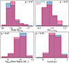 |
Fig. 14. Distributions of peak ZTFg-band magnitude, Δm15 in ZTFg, host galaxy mass, and local g-r colour for the HVF and non-HVF subsets of the 190 SNe low-bias sample. The means of each distribution are displayed as the dotted lines with the KS test p-values indicated in each panel. |
The host galaxy mass and local g-r colour (Smith et al., in prep.) are shown in the bottom panels of Fig. 14. The p-values for the host mass and local colour distributions of the HVF and non-HVF samples are large relative to the 0.05 threshold, with values of 0.65 and 0.59, respectively, again consistent with a lack of a difference in the local environment between SNe Ia with and without a Si IIλ6355 HVF.
As before for investigating trends with x1, we repeated these statistical tests exclusively with spectra before –8.7 d. We once again found large p-values for peak absolute magnitude and Δm15 in the ZTFg-band (0.91 and 0.52) as well as for the host galaxy mass and local g-r colour (1.0 and 0.94), indicating no difference between the HVF and non-HVF populations in these observables.
5. Discussion
In Sect. 5.1 we discuss our results in the context of the results of the literature, particularly those of Silverman et al. (2015). In Sect. 5.2 we investigate the potential false classification rates of the ‘Wang’ (Wang et al. 2009) and the ‘Branch’ (Branch et al. 2006, 2009), classification schemes if HVFs are not taken into account. Finally, we compare our velocity distributions to hydrodynamical explosion models in Sect. 5.3.
5.1. Comparison to literature
Silverman et al. (2015) investigated the properties of SNe Ia both with and without HVF in the context of the velocity-based classification scheme of Wang et al. (2009). The ‘Wang classification scheme’ divides objects into normal-velocity (NVW) and high-velocity (HVW) subclasses depending on whether the photospheric velocity (measured from the Si IIλ6355 feature) is less than or greater than 11 800 km s−1 around peak (–5 to 5 d), respectively. We chose to add the ‘W’ subscript here to differentiate between the high-velocity Wang subclass (HVW) and the high-velocity components (HV). While the cut-off of 11 800 km s−1 was employed by Silverman et al. (2015), we chose to adopt a cut-off of 12 000 km s−1 for consistency with other ZTF DR2 studies (Burgaz et al. 2025). Our Wang classifications are drawn from the latest spectrum we have for each object. In the case of the HVW class, only spectra later that –5 d were used. However, for any object for which the latest pre-peak spectrum has PV < 12 000 km s−1, regardless of phase, we denote it as NVW as the photospheric velocity is not expected to increase and the objects will still have photospheric velocities below 12 000 km s−1 around peak. These classifications are then augmented by classifications from (Burgaz et al. 2025) for which they examined a slightly later phase range of –5 to 5 d with respect to peak brightness.
Figure 15 presents the pEW ratio, RHVF, against the photospheric velocity of the Si IIλ6355 feature for the low-bias sample of 190 SNe Ia. When investigating the same parameters, Silverman et al. (2015) found a dearth of NVW SNe exhibiting HVFs in the Si IIλ6355 (RHVF > 0), with these features found more predominantly in HVW SNe. Contrary to this, we find HVFs in 26 of the NVW classified objects in our low-bias sample (36 in the full sample), largely populating the empty region of the parameter space seen by Silverman et al. (2015). An increase in RHVF with increasing photospheric velocity was also observed by Silverman et al. (2015). While this correlation makes intuitive sense for the evolution of individual objects, with RHVF and photospheric velocity both decreasing over time, we observe no such global correlation in Fig. 15. As before with the lack of a global downwards trend in the middle panel of Fig. 9, this indicates that the onset of the RHVF evolution begins at different phases for different objects.
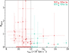 |
Fig. 15. Ratio of the pseudo-equivalent widths of the HV and PV components against the photospheric velocity of the Si IIλ6355 feature for the low-bias sample of 190 SNe. For objects with multiple spectra we take the mean value in both dimensions, treating the uncertainties with the ASYMMETRIC UNCERTAINTY package (Gobat 2022). The vertical dotted line indicates the 12 000 km s−1 cut velocity at maximum light between the NVW (red) and HVW (green) SNe Ia. |
5.2. Wang and Branch reclassifications
As described above, Wang classifications (NVW versus. HVW) are generally measured using the Si IIλ6355 photospheric velocity in the phase range –5 to 5 d with respect to peak. However, the specific measurement of this velocity will change depending upon whether we employ a single- or a double-component model. Historically this feature has been treated as a single component around peak, believed to be free of any HV components. However, our study, as well as the results from Silverman et al. (2015), suggests that HV components might be more common at these phases (later than –5 d) than previously thought, with one third of SN Ia spectra between –5 d and peak displaying an HVF. Therefore, we pose the question, if in these large spectroscopic studies we were to consider and account for HV Si IIλ6355 absorption close to maximum light, what percentage of the HVW classifications would be overturned in favour of a NVW subtype?
In the top panel of Fig. 16, we compare the photospheric velocity from the single component fits against the ‘true’ photospheric velocities (i.e. single component fits for spectra without an HVF, and double component fits for spectra with an HVF). All spectra identified to have an HV component exhibit lower photospheric velocities in their two-component fits as would be expected. We indicate the Wang classification cut off velocity of 12 000 km s−1 by the vertical and horizontal dotted lines, highlighting the region in the bottom right in which the objects would be classified as HVW with the single component model, but as NVW by the double-component model (orange points). When considering the 85 objects from the low-bias sample that possess a spectrum later than –5 d, there are five SNe Ia (seven of the 150 SNe from the full sample with a spectrum later than –5 d), indicating that  % of HVW classifications (
 % for the full sample) before peak would be incorrect if we were to not consider HV components. These uncertainties represent 68% confidence intervals and are calculated as binomial with the Clopper-Pearson interval. Such large uncertainties are the result of low number statistics and while this leaves the percentages fairly unconstrained, this suggests that HVF components could cause a significant rate of false HVW classifications in the 5 d before maximum light.
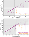 |
Fig. 16. Comparison of the photospheric velocity (top) and pEW (bottom) measured using the single component fits against taking into consideration the HV components and using the two component fits wherever an HV component was identified. Solid data points represent the low-bias sample, with hollow data points corresponding to the remaining objects from the full sample with z > 0.06. The points indicated in orange would be misclassified in the Wang scheme and Branch scheme in the top and bottom panels respectively, if the HV components were not to be considered. These two classification schemes concern spectra around maximum light, and as such, all the spectra presented here have phases greater that –5 d. |
Similarly, we performed this analysis with respect to the Branch classification scheme (Branch et al. 2006, 2009), which divides up the SN Ia population based upon the equivalent widths of the Si IIλ6355 and Si IIλ5972 lines. Broad-line (BL) SNe Ia exhibit pEWSi 6355 > 105 Å with a pEWSi 5972 < 30 Å. While we have no information on the Si IIλ5972, we can examine the effects of HV components upon the measured Si IIλ6355 pEW. The bottom panel of Fig. 16 displays the measured photospheric pEW coming from the single component fits against the ‘true’ photospheric pEWs (as above for the Wang analysis). The cut-off width at 105 Å is indicated by the dotted lines, with the orange points once again corresponding to those spectra that would receive an incorrect classification if we were to not consider the HV components. In the Branch scheme parameter space there are four SNe that are misclassified (six for the full sample), resulting in  % of incorrect BL classifications (
 % for the full sample) with respect to the Si IIλ6355 line. In their sample of BL SNe Ia, Yarbrough et al. (2023) also find the BL population to have higher Si IIλ6355 velocities than their core normal (CN) counterparts, further supporting this idea as the HV components would also cause an offset in measured single component velocities to higher values. These uncertainties represent 68% intervals as before for the Wang reclassifications, and once again the low number of data points results in loosely constrained percentages.
With generally smaller velocity separations in this phase range around peak, false positives are more probable and could have the inverse effect in both these cases. Incorrectly employing a double-component model to a Si IIλ6355 feature with no HVF would artificially decrease the photospheric velocity and width, potentially resulting in HVW SNe being classified as NVW and Branch BL SNe being missed. Therefore, the misclassification rates calculated here represent upper limits.
5.3. HVF origins
While the specific origins and formation channels of these HV components of the Si IIλ6355 feature remain unclear, they provide clear evidence of intermediate-mass element material in the upper ejecta of the majority of SNe Ia. Regardless of the explosion mechanism or progenitor channel, any model aiming to reproduce these features will require some fraction of silicon at the corresponding high velocities.
In Fig. 17 we present the measured velocity distributions for the PV and HV components for the HVF classified spectra in our sample, with the Si-abundance profiles from a number of explosion models from the Heidelberg Supernova Model Archive (HESMA; Kromer et al. 2017), arising from three different explosion mechanisms. In pink we plot the delayed-detonation (DDT) models (Röpke et al. 2012; Seitenzahl et al. 2013; Ohlmann et al. 2014) arising from an initial subsonic deflagration that later transitions to a supersonic detonation. In blue, we plot the double-detonation models (Sim et al. 2012; Gronow et al. 2020, 2021), which involves a detonation in a helium shell atop the white dwarf, sending a shock-wave inwards that converges in – and subsequently detonates – the core. Finally, in yellow we show the silicon abundances from the pure subsonic deflagration models (Fink et al. 2014; Kromer et al. 2015).
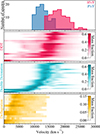 |
Fig. 17. Comparison of the measured velocity distributions of PV and HV components in our sample for spectra identified as having both components (top) against the distributions of silicon from a number of theoretical explosion models from the HESMA archive (Kromer et al. 2017). Each of the three panels corresponds to a different explosion mechanism, with each row of the colour plot as an individual, unique model. |
As expected, the pure deflagration models are very homogeneous in nature, possessing very flat distributions of the elements in the model. In addition, as a result of the low energy, they do not produce material moving at velocities faster than around 15 000 km s−1 and are therefore incapable of producing the HV – and many of the PV – components that can be seen in the DR2. The DDT and double-detonation models possess more layered ejecta structures, with peaks in the silicon abundance profiles in the 10 000–15 000 km s−1 range. The majority of these models also exhibit silicon at velocities covering the full HVF velocity distribution. The formation of such HVFs is dependant upon the ionisation profile, which in turn is dependant upon not only the abundances, but also the density profile of the plasma. This will be the focus of a follow-up modelling study with a handful of well-sampled HVF objects (Harvey et al., in prep.).
We also note here that the models presented in Fig. 17 are designed to reproduce the overall SN Ia photometric and spectroscopic evolution coming from the primary white dwarf itself. These HVFs may instead be the result of environmental components such as CSM, which are not included in the models. Through the spectroscopic modelling of the HVFs exhibited by SN 1999ee, Mazzali et al. (2005b) explored the ejecta conditions needed to recreate the evolution. In terms of an abundance enhancement, they required a region of the upper ejecta to be dominated by silicon and calcium (∼90 and ∼10% respectively), which is hard to justify in terms of nuclear burning. Therefore, they concluded that density enhancements in these regions are a more plausible cause of the HVFs. In Mazzali et al. (2005a), they suggested the sweeping up of surrounding CSM to be responsible for the line-forming region higher up in the ejecta, pointing to a thick disc and/or high density CSM environment produced by a companion wind. They also proposed angular fluctuations as a potential cause of density enhancement, with HVFs being the result of three-dimensional effects. This was further supported by Tanaka et al. (2006) who investigated various density enhancement geometries and degrees of photospheric coverage to produce the observed HVF population. This multidimensional requirement is supported by the observed polarisation difference between the HV and PV components of the Ca NIR triplet in SN 2001el (Wang et al. 2003; Kasen et al. 2003) and in the Si IIλ6355 of SN 2019ein/ZTF19aatlmbo (Patra et al. 2022).
6. Conclusions
In this work, we have conducted a thorough search for Si IIλ6355 HV components within the ZTF Cosmology Data Release 2 by way of MCMC fitting and model selection with the BIC. Through simulations, we quantified the detection efficiency over the spectral quality (S/N and dispersion) as well as for simulated velocity separation between the two components. These simulations were also employed to test the accuracy of the estimated uncertainties and identify and correct the biases in the model parameters. Within our sample of 329 spectra, we identified 85 Si IIλ6355 HV components. We subsequently defined a low-bias subsample with a redshift cut at 0.06 (210 spectra from 190 SNe) that was then used to calculate rates. Our conclusions from the analysis are as follows:
-
Of the spectra,
 % before –11 d exhibit HVFs in the Si IIλ6355 feature. This percentage dropped as we approached maximum light, with 29 ± 5% of spectra showing HVFs after –6 d.
 -
For individual objects, we observed a decrease in the HVF strength ratio RHVF with time, corresponding to the fading away of the HV component and leaving just the PV absorption. This evolution occurs at different phases for different objects, and therefore, globally, we observed a relatively uniform distribution of RHVF with phase.
-
The HV components with larger separations from their PV counterparts fade at earlier epochs, leaving just the smaller separations as we approached maximum light. We did not observe consistent Δv evolution from object to object, with some increasing, others decreasing, and some remaining constant.
-
We observed no tendency of Si IIλ6355 HVFs to occur in objects with high or low SALT x1 values, supporting the proposed ubiquity of HVFs across the SN Ia class.
-
Comparison of a low-bias subsample of our targets with the volume-limited DR2 sample (defined as a control sample) showed no statistical difference between the HVF and non-HVF populations in ZTFg-band peak magnitude and Δm15(ZTFg), host mass, or local host g-r colour.
-
We do not reproduce the finding from Silverman et al. (2015) that the Wang classification scheme HVW objects are more likely to exhibit Si IIλ6355 HVFs. A fairly significant portion of our HVF spectra come from NVW objects.
-
The fitting of Si IIλ6355 profiles without consideration of contributions from potential HV components may cause a number of false HVW classifications. We calculated an upper limit for the false HVW classification rate of
 % in the phase range –5 to 0 d.
 -
Similarly, for the Branch classification scheme, we find that up to
 % of the BL classifications drawn from spectra in the phase range –5 to 0 d are incorrect, as unaccounted HV components broaden the feature.
To summarise, our analysis provides detailed insights into the behaviour of HV components in SNe Ia. These findings support the previously proposed ubiquity of HVFs across the SN Ia population, underscore the importance of considering HV components when interpreting spectral data, and provide a foundation for future studies investigating the nature and impact of HVFs in SNe Ia. Further investigation would be required from a modelling standpoint to shed light upon the specific mechanisms giving rise to HVFs and the characteristics found here.
Data availability
The feature measurements for all 329 spectra are available in electronic form at the CDS via anonymous ftp to cdsarc.cds.unistra.fr (130.79.128.5) or via http://cdsweb.u-strasbg.fr/cgi-bin/qcat?J/A+A/695/A264. For other measurements presented in this paper – light curve properties, Branch and Wang classifications, host galaxy properties – we refer the reader to the source papers (Dimitriadis et al. 2025; Burgaz et al. 2025; Smith et al., in prep.).
FLOYDS_PIPELINE, https://github.com/svalenti/floyds_pipeline
FORSIFY, https://github.com/afloers/forsify
IRAF was distributed by the National Optical Astronomy Observatory, which is operated by the Association of Universities for Research in Astronomy, Inc., under cooperative agreement with the National Science Foundation.
Acknowledgments
The research conducted in this publication was funded by the Irish Research Council under grant number GOIPG/2020/1387. K.M., U.B., G.D., M.D., and J.T. acknowledge support from EU H2020 ERC grant no. 758638. L.G. acknowledges financial support from the Spanish Ministerio de Ciencia e Innovación (MCIN), the Agencia Estatal de Investigación (AEI) 10.13039/501100011033, and the European Social Fund (ESF) "Investing in your future" under the 2019 Ramón y Cajal program RYC2019-027683-I and the PID2020-115253GA-I00 HOSTFLOWS project, from Centro Superior de Investigaciones Científicas (CSIC) under the PIE project 20215AT016, and the program Unidad de Excelencia María de Maeztu CEX2020-001058-M. Y.-L.K. has received funding from the Science and Technology Facilities Council [grant number ST/V000713/1]. This project has received funding from the European Research Council (ERC) under the European Union’s Horizon 2020 research and innovation programme (grant agreement n°759194 – USNAC). This work has been supported by the research project grant “Understanding the Dynamic Universe” funded by the Knut and Alice Wallenberg Foundation under Dnr KAW 2018.0067, Vetenskapsrådet, the Swedish Research Council, project 2020-03444. Based on observations obtained with the Samuel Oschin Telescope 48-inch and the 60-inch Telescope at the Palomar Observatory as part of the Zwicky Transient Facility project. ZTF is supported by the National Science Foundation under Grant No. AST-1440341 and a collaboration including Caltech, IPAC, the Weizmann Institute of Science, the Oskar Klein Center at Stockholm University, the University of Maryland, the University of Washington, Deutsches Elektronen-Synchrotron and Humboldt University, Los Alamos National Laboratories, the TANGO Consortium of Taiwan, the University of Wisconsin at Milwaukee, and Lawrence Berkeley National Laboratories. Operations are conducted by COO, IPAC, and UW. This work was supported by the GROWTH project (Kasliwal et al. 2019) funded by the National Science Foundation under Grant No 1545949. The SALT classification spectra of SN 2020lil and SN 2020pst were obtained through Rutgers University program 2020-1-MLT-007 (PI: S. W. Jha). Based on observations collected at the European Organisation for Astronomical Research in the Southern Hemisphere under ESO programmes 199.D-0143, 1103.D-0328, and 106.216C.009. The authors thank Michael Tucker for advising in the quality and inclusion of SNIFS/UH-88 spectra from the SCAT survey. Based on observations collected at Copernico 1.82m telescope (Asiago Mount Ekar, Italy) INAF – Osservatorio Astronomico di Padova. The data presented here were obtained in part with ALFOSC, which is provided by the Instituto de Astrofisica de Andalucia (IAA) under a joint agreement with the University of Copenhagen and NOT. Some of the data presented herein were obtained at Keck Observatory, which is a private 501(c)3 non-profit organization operated as a scientific partnership among the California Institute of Technology, the University of California, and the National Aeronautics and Space Administration. The Observatory was made possible by the generous financial support of the W. M. Keck Foundation. The authors wish to recognize and acknowledge the very significant cultural role and reverence that the summit of Maunakea has always had within the Native Hawaiian community. We are most fortunate to have the opportunity to conduct observations from this mountain. Based on observations obtained with the Apache Point Observatory 3.5-meter telescope, which is owned and operated by the Astrophysical Research Consortium. This article is based on observations made with the Gran Telescopio Canarias operated by the Instituto de Astrofisica de Canarias, the Isaac Newton Telescope, and the William Herschel Telescope operated by the Isaac Newton Group of Telescopes, the Italian Telescopio Nazionale Galileo operated by the Fundacion Galileo Galilei of the INAF (Istituto Nazionale di Astrofisica), and the Liverpool Telescope operated by Liverpool John Moores University with financial support from the UK Science and Technology Facilities Council. All these facilities are located at the Spanish Roque de los Muchachos Observatory of the Instituto de Astrofisica de Canarias on the island of La Palma. Based on observations collected at the European Organisation for Astronomical Research in the Southern Hemisphere. This work makes use of observations from the Las Cumbres Observatory global telescope network. Based on observations obtained at the international Gemini Observatory, a program of NSF’s NOIRLab, which is managed by the Association of Universities for Research in Astronomy (AURA) under a cooperative agreement with the National Science Foundation on behalf of the Gemini Observatory partnership: the National Science Foundation (United States), National Research Council (Canada), Agencia Nacional de Investigación y Desarrollo (Chile), Ministerio de Ciencia, Tecnología e Innovación (Argentina), Ministério da Ciência, Tecnologia, Inovações e Comunicações (Brazil), and Korea Astronomy and Space Science Institute (Republic of Korea). Based on observations obtained at the Southern Astrophysical Research (SOAR) telescope, which is a joint project of the Ministério da Ciência, Tecnologia e Inovações (MCTI/LNA) do Brasil, the US National Science Foundation’s NOIRLab, the University of North Carolina at Chapel Hill (UNC), and Michigan State University (MSU). This paper includes data gathered with the 6.5 meter Magellan Telescopes located at Las Campanas Observatory, Chile. These results made use of the Lowell Discovery Telescope (LDT) at Lowell Observatory. Lowell is a private, non-profit institution dedicated to astrophysical research and public appreciation of astronomy and operates the LDT in partnership with Boston University, the University of Maryland, the University of Toledo, Northern Arizona University and Yale University. The Large Monolithic Imager was built by Lowell Observatory using funds provided by the National Science Foundation (AST-1005313). The upgrade of the DeVeny optical spectrograph has been funded by a generous grant from John and Ginger Giovale and by a grant from the Mt. Cuba Astronomical Foundation. Some of the observations reported in this paper were obtained with the Southern African Large Telescope (SALT). This work made use of the Heidelberg Supernova Model Archive (HESMA), https://hesma.h-its.org.
References
- Aldering, G., Adam, G., Antilogus, P., et al. 2002, in Survey and Other Telescope Technologies and Discoveries, eds. J. A. Tyson, & S. Wolff, Society of Photo-Optical Instrumentation Engineers (SPIE) Conference Series, 4836, 61 [NASA ADS] [CrossRef] [Google Scholar]
- Allington-Smith, J., Murray, G., Content, R., et al. 2002, PASP, 114, 892 [NASA ADS] [CrossRef] [Google Scholar]
- Barnsley, R., Smith, R., & Steele, I. 2012, in Astronomical Data Analysis Software and Systems XXI, eds. P. Ballester, D. Egret, & N. P. F. Lorente, Astronomical Society of the Pacific Conference Series, 461, 517 [NASA ADS] [Google Scholar]
- Bellm, E. C., & Sesar, B. 2016, Astrophysics Source Code Library [record ascl:1602.002] [Google Scholar]
- Bellm, E. C., Kulkarni, S. R., Graham, M. J., et al. 2019, PASP, 131, 018002 [Google Scholar]
- Benetti, S., Cappellaro, E., Mazzali, P. A., et al. 2005, ApJ, 623, 1011 [NASA ADS] [CrossRef] [Google Scholar]
- Benn, C., Dee, K., & Agócs, T. 2008, in Ground-based and Airborne Instrumentation for Astronomy II, eds. I. S. McLean, & M. M. Casali, Society of Photo-Optical Instrumentation Engineers (SPIE) Conference Series, 7014, 70146X [Google Scholar]
- Blagorodnova, N., Neill, J. D., Walters, R., et al. 2018, PASP, 130, 035003 [Google Scholar]
- Blondin, S., Mandel, K. S., & Kirshner, R. P. 2011, A&A, 526, A81 [NASA ADS] [CrossRef] [EDP Sciences] [Google Scholar]
- Branch, D., Dang, L. C., Hall, N., et al. 2006, PASP, 118, 560 [NASA ADS] [CrossRef] [Google Scholar]
- Branch, D., Chau Dang, L., & Baron, E. 2009, PASP, 121, 238 [NASA ADS] [CrossRef] [Google Scholar]
- Brown, T. M., Baliber, N., Bianco, F. B., et al. 2013, PASP, 125, 1031 [Google Scholar]
- Buckley, D. A. H., Swart, G. P., & Meiring, J. G. 2006, in Ground-based and Airborne Telescopes, ed. L. M. Stepp, Society of Photo-Optical Instrumentation Engineers (SPIE) Conference Series, 6267, 62670Z [NASA ADS] [CrossRef] [Google Scholar]
- Burgaz, U., Maguire, K., Dimitriadis, G., et al. 2025, A&A, 694, A9 [NASA ADS] [CrossRef] [EDP Sciences] [Google Scholar]
- Buzzoni, B., Delabre, B., Dekker, H., et al. 1984, Messenger, 38, 9 [Google Scholar]
- Cenko, S. B., Fox, D. B., Moon, D.-S., et al. 2006, PASP, 118, 1396 [Google Scholar]
- Cepa, J., Aguiar, M., Escalera, V. G., et al. 2000, in Optical and IR Telescope Instrumentation and Detectors, eds. M. Iye, & A. F. Moorwood, Society of Photo-Optical Instrumentation Engineers (SPIE) Conference Series, 4008, 623 [NASA ADS] [CrossRef] [Google Scholar]
- Childress, M. J., Scalzo, R. A., Sim, S. A., et al. 2013, ApJ, 770, 29 [NASA ADS] [CrossRef] [Google Scholar]
- Childress, M. J., Filippenko, A. V., Ganeshalingam, M., & Schmidt, B. P. 2014, MNRAS, 437, 338 [CrossRef] [Google Scholar]
- Clemens, J. C., Crain, J. A., & Anderson, R. 2004, in Ground-based Instrumentation for Astronomy, eds. A. F. M. Moorwood, & M. Iye, Society of Photo-Optical Instrumentation Engineers (SPIE) Conference Series, 5492, 331 [NASA ADS] [CrossRef] [Google Scholar]
- Crawford, S. M., Still, M., Schellart, P., et al. 2010, in Observatory Operations: Strategies, Processes, and Systems III, eds. D. R. Silva, A. B. Peck, & B. T. Soifer, Society of Photo-Optical Instrumentation Engineers (SPIE) Conference Series, 7737, 773725 [NASA ADS] [CrossRef] [Google Scholar]
- Das, K. K., Kasliwal, M. M., Fremling, C., et al. 2023, ApJ, 959, 12 [CrossRef] [Google Scholar]
- Dekany, R., Smith, R. M., Riddle, R., et al. 2020, PASP, 132, 038001 [NASA ADS] [CrossRef] [Google Scholar]
- Dimitriadis, G., Foley, R. J., Arendse, N., et al. 2022, ApJ, 927, 78 [NASA ADS] [CrossRef] [Google Scholar]
- Dimitriadis, G., Burgaz, U., Deckers, M., et al. 2025, A&A, 694, A10 [NASA ADS] [CrossRef] [EDP Sciences] [Google Scholar]
- Dressler, A., Bigelow, B., Hare, T., et al. 2011, PASP, 123, 288 [NASA ADS] [CrossRef] [Google Scholar]
- Fink, M., Kromer, M., Seitenzahl, I. R., et al. 2014, MNRAS, 438, 1762 [NASA ADS] [CrossRef] [Google Scholar]
- Foreman-Mackey, D., Hogg, D. W., Lang, D., & Goodman, J. 2013, PASP, 125, 306 [Google Scholar]
- Gerardy, C. L., Höflich, P., Fesen, R. A., et al. 2004, ApJ, 607, 391 [Google Scholar]
- Gobat, C. 2022, Astrophysics Source Code Library [record ascl:2208.005] [Google Scholar]
- Graham, M. J., Kulkarni, S. R., Bellm, E. C., et al. 2019, PASP, 131, 078001 [Google Scholar]
- Gronow, S., Collins, C., Ohlmann, S. T., et al. 2020, A&A, 635, A169 [NASA ADS] [CrossRef] [EDP Sciences] [Google Scholar]
- Gronow, S., Collins, C. E., Sim, S. A., & Röpke, F. K. 2021, A&A, 649, A155 [NASA ADS] [CrossRef] [EDP Sciences] [Google Scholar]
- Guy, J., Astier, P., Baumont, S., et al. 2007, A&A, 466, 11 [NASA ADS] [CrossRef] [EDP Sciences] [Google Scholar]
- Hamuy, M., Folatelli, G., Morrell, N. I., et al. 2006, PASP, 118, 2 [NASA ADS] [CrossRef] [Google Scholar]
- Hatano, K., Branch, D., Fisher, A., Baron, E., & Filippenko, A. V. 1999, ApJ, 525, 881 [NASA ADS] [CrossRef] [Google Scholar]
- Hook, I. M., Jørgensen, I., Allington-Smith, J. R., et al. 2004, PASP, 116, 425 [NASA ADS] [CrossRef] [Google Scholar]
- Hung, T., Gezari, S., Blagorodnova, N., et al. 2017, ApJ, 842, 29 [NASA ADS] [CrossRef] [Google Scholar]
- Kasen, D., Nugent, P., Wang, L., et al. 2003, ApJ, 593, 788 [NASA ADS] [CrossRef] [Google Scholar]
- Kasliwal, M. M., Cannella, C., Bagdasaryan, A., et al. 2019, PASP, 131, 038003 [NASA ADS] [CrossRef] [Google Scholar]
- Kim, Y. L., Rigault, M., Neill, J. D., et al. 2022, PASP, 134, 024505 [NASA ADS] [CrossRef] [Google Scholar]
- Kobulnicky, H. A., Nordsieck, K. H., Burgh, E. B., et al. 2003, in Instrument Design and Performance for Optical/Infrared Ground-based Telescopes, eds. M. Iye, & A. F. M. Moorwood, Society of Photo-Optical Instrumentation Engineers (SPIE) Conference Series, 4841, 1634 [Google Scholar]
- Kochanek, C. S., Shappee, B. J., Stanek, K. Z., et al. 2017, PASP, 129, 104502 [Google Scholar]
- Kromer, M., Ohlmann, S. T., Pakmor, R., et al. 2015, MNRAS, 450, 3045 [NASA ADS] [CrossRef] [Google Scholar]
- Kromer, M., Ohlmann, S., & Röpke, F. K. 2017, Mem. Soc. Astron. It., 88, 312 [NASA ADS] [Google Scholar]
- Lezmy, J., Copin, Y., Rigault, M., Smith, M., & Neill, J. D. 2022, A&A, 668, A43 [NASA ADS] [CrossRef] [EDP Sciences] [Google Scholar]
- Maguire, K., Sullivan, M., Pan, Y. C., et al. 2014, MNRAS, 444, 3258 [NASA ADS] [CrossRef] [Google Scholar]
- Marion, G. H., Vinko, J., Wheeler, J. C., et al. 2013, ApJ, 777, 40 [Google Scholar]
- Masci, F. J., Laher, R. R., Rusholme, B., et al. 2019, PASP, 131, 018003 [Google Scholar]
- Mazzali, P. A., Benetti, S., Altavilla, G., et al. 2005a, ApJ, 623, L37 [NASA ADS] [CrossRef] [Google Scholar]
- Mazzali, P. A., Benetti, S., Stehle, M., et al. 2005b, MNRAS, 357, 200 [NASA ADS] [CrossRef] [Google Scholar]
- McCarthy, J. K., Cohen, J. G., Butcher, B., et al. 1998, in Optical Astronomical Instrumentation, ed. S. D’Odorico, Society of Photo-Optical Instrumentation Engineers (SPIE) Conference Series, 3355, 81 [Google Scholar]
- Miller, J. S., & Stone, R. P. S. 1993, in Lick Observatory technical Report 66 (Santa Cruz, CA: Lick Observatory) [Google Scholar]
- Nordin, J., Östman, L., Goobar, A., et al. 2011, A&A, 526, A119 [NASA ADS] [CrossRef] [EDP Sciences] [Google Scholar]
- Ohlmann, S. T., Kromer, M., Fink, M., et al. 2014, A&A, 572, A57 [NASA ADS] [CrossRef] [EDP Sciences] [Google Scholar]
- Oke, J. B., Cohen, J. G., Carr, M., et al. 1995, PASP, 107, 375 [Google Scholar]
- Patra, K. C., Yang, Y., Brink, T. G., et al. 2022, MNRAS, 509, 4058 [Google Scholar]
- Pedregosa, F., Varoquaux, G., Gramfort, A., et al. 2011, J. Mach. Learn. Res., 12, 2825 [Google Scholar]
- Perley, D. A. 2019, PASP, 131, 084503 [Google Scholar]
- Perlmutter, S., Aldering, G., Goldhaber, G., et al. 1999, ApJ, 517, 565 [Google Scholar]
- Phillips, M. M. 1993, ApJ, 413, L105 [Google Scholar]
- Piascik, A. S., Steele, I. A., Bates, S. D., et al. 2014, in Ground-based and Airborne Instrumentation for Astronomy V, eds. S. K. Ramsay, I. S. McLean, & H. Takami, Society of Photo-Optical Instrumentation Engineers (SPIE) Conference Series, 9147, 91478H [NASA ADS] [Google Scholar]
- Prentice, S. J., Maguire, K., Smartt, S. J., et al. 2018, ApJ, 865, L3 [NASA ADS] [CrossRef] [Google Scholar]
- Prochaska, J., Hennawi, J., Westfall, K., et al. 2020, J. Open Source Softw., 5, 2308 [NASA ADS] [CrossRef] [Google Scholar]
- Pskovskii, I. P. 1977, Soviet Ast., 21, 675 [Google Scholar]
- Quimby, R., Höflich, P., Kannappan, S. J., et al. 2006, ApJ, 636, 400 [NASA ADS] [CrossRef] [Google Scholar]
- Riess, A. G., Filippenko, A. V., Challis, P., et al. 1998, AJ, 116, 1009 [Google Scholar]
- Rigault, M., Neill, J. D., Blagorodnova, N., et al. 2019, A&A, 627, A115 [NASA ADS] [CrossRef] [EDP Sciences] [Google Scholar]
- Rigault, M., Smith, M., Goobar, A., et al. 2025, A&A, 694, A1 [NASA ADS] [CrossRef] [EDP Sciences] [Google Scholar]
- Rockosi, C., Stover, R., Kibrick, R., et al. 2010, in Ground-based and Airborne Instrumentation for Astronomy III, eds. I. S. McLean, S. K. Ramsay, & H. Takami, Society of Photo-Optical Instrumentation Engineers (SPIE) Conference Series, 7735, 77350R [NASA ADS] [Google Scholar]
- Röpke, F. K., Kromer, M., Seitenzahl, I. R., et al. 2012, ApJ, 750, L19 [CrossRef] [Google Scholar]
- Seitenzahl, I. R., Ciaraldi-Schoolmann, F., Röpke, F. K., et al. 2013, MNRAS, 429, 1156 [NASA ADS] [CrossRef] [Google Scholar]
- Sharma, Y., Sollerman, J., Fremling, C., et al. 2023, ApJ, 948, 52 [NASA ADS] [CrossRef] [Google Scholar]
- Silverman, J. M., Kong, J. J., & Filippenko, A. V. 2012, MNRAS, 425, 1819 [NASA ADS] [CrossRef] [Google Scholar]
- Silverman, J. M., Vinkó, J., Marion, G. H., et al. 2015, MNRAS, 451, 1973 [CrossRef] [Google Scholar]
- Sim, S. A., Fink, M., Kromer, M., et al. 2012, MNRAS, 420, 3003 [NASA ADS] [CrossRef] [Google Scholar]
- Smartt, S. J., Valenti, S., Fraser, M., et al. 2015, A&A, 579, A40 [NASA ADS] [CrossRef] [EDP Sciences] [Google Scholar]
- Smith, K. W., Smartt, S. J., Young, D. R., et al. 2020, PASP, 132, 085002 [Google Scholar]
- Steele, I. A., Smith, R. J., Rees, P. C., et al. 2004, in Ground-based Telescopes, eds. J. Oschmann, & M. Jacobus, Society of Photo-Optical Instrumentation Engineers (SPIE) Conference Series, 5489, 679 [NASA ADS] [CrossRef] [Google Scholar]
- Stevenson, K. B., Bean, J. L., Seifahrt, A., et al. 2016, ApJ, 817, 141 [NASA ADS] [CrossRef] [Google Scholar]
- Tanaka, M., Mazzali, P. A., Maeda, K., & Nomoto, K. 2006, ApJ, 645, 470 [Google Scholar]
- Taubenberger, S. 2017, in Handbook of Supernovae, eds. A. W. Alsabti, & P. Murdin, 317 [CrossRef] [Google Scholar]
- Thomas, R. C., Branch, D., Baron, E., et al. 2004, ApJ, 601, 1019 [Google Scholar]
- Tonry, J. L., Denneau, L., Heinze, A. N., et al. 2018, PASP, 130, 064505 [Google Scholar]
- Tucker, M. A., Shappee, B. J., Huber, M. E., et al. 2022, PASP, 134, 124502 [NASA ADS] [CrossRef] [Google Scholar]
- Valenti, S., Sand, D., Pastorello, A., et al. 2014, MNRAS, 438, L101 [Google Scholar]
- Wang, L., Baade, D., Höflich, P., et al. 2003, ApJ, 591, 1110 [Google Scholar]
- Wang, X., Filippenko, A. V., Ganeshalingam, M., et al. 2009, ApJ, 699, L139 [NASA ADS] [CrossRef] [Google Scholar]
- Yarbrough, Z., Baron, E., DerKacy, J. M., et al. 2023, MNRAS, 521, 3873 [NASA ADS] [Google Scholar]
Appendix A: Supplementary photometry
Our initial light curve quality cut was employed as a general guideline to remove any supernovae from our sample with a poor corresponding SALT fit. A total of 2954 supernovae from the 3585 met this criteria. For completeness, these 2954 light curves were visually inspected, leading to the identification of 13 poorly sampled light curves that resulted in spectral phase estimates that were unrealistically early (< − 20 d). Supplementary forced photometry for these objects was obtained from the Asteroid Terrestrial-impact Last Alert System (ATLAS; Tonry et al. 2018; Smith et al. 2020), leading to more reliable estimates of t0.
Of the 631 objects that do not meet the initial criteria, there are a number with SALT fits acceptable enough with respect to t0 from which we can accurately estimate a spectral phase. Through visual inspection, we identified 255 such objects, and they were then added to the sample.
For the remaining 376 targets, we scraped as many forced photometry light curves as possible from ATLAS. If an ATLAS light curve could not be located, we instead attempted to scrape photometry from the All-Sky Automated Survey for Supernovae (ASAS-SN; Kochanek et al. 2017). In total this search returned 197 light curves from ATLAS and 2 from ASAS-SN. We fit these supplementary light curves with SALT and inspected the fits by eye. In the case of a successful SALT fit to this additional data that produces a well-constrained estimate of maximum light, we ‘accepted’ the supplementary SALT fit. In total, we accepted the updated t0 values for 84 of these objects (82 from ATLAS and 2 from ASAS-SN).
We set an errorfloor of 1.0 d on the t0 value for any object that required supplementary photometry and/or did not meet the initial criteria laid out in Sect. 2. We note here that while these objects are included in the sample at this point, the corresponding spectra may be removed subject to one of the various cuts that follow. Any spectra in the final sample corresponding to objects with these updated phases are excluded from any plots and analyses relating to light curve fit parameters other than t0 (x1, c). All updated peak MJD values coming from supplementary photometry can be found in Table A.1.
Figure A.1 illustrates one such example of an updated t0 estimate. As visible in the plot, there are only three ZTF photometry points for ZTF19abjkfrf, in a single band, post-peak. Due to the poor phase coverage of the light curve, this object will be excluded from almost all studies, especially those concerning cosmological measurements. As we possess a good quality pre-peak spectrum, however, updating the phase estimate in this fashion allowed us to avoid cutting otherwise acceptable data. For this object the phase estimate has changed from −35.9 to −12.5 d. The updated estimates for t0 for the 92 supernovae in Table A.1 were subsequently used to as initial constraints in refitting the corresponding light curves for the DR2.
Updated maximum light values from supplementary photometric data for improved spectral phase estimation.
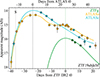 |
Fig. A.1. An example of a SALT2 fit to a DR2 g-band light curve of ZTF19abjkfrf, which results in a poor spectral phase estimate due to low coverage and single-band data. The original SALT2 fit is shown in green with the updated fit to the supplementary data from ATLAS in the cyan (ATLASc) and orange (ATLASo) filters displayed by the cyan and orange curves. The spectral date is represented by the solid grey vertical line, with the dotted vertical lines corresponding to the original (green) and updated (black) maximum light fit measurements. |
Appendix B: Two-component fits
The two component fits to the 85 spectra identified as exhibiting Si IIλ6355 HVFs are presented in Fig. B.1.
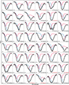 |
Fig. B.1. Best fits to the 85 ZTF DR2 spectra in the sample identified as having an HV component. The phase and SN ZTF name are indicated in each panel. The continuum regions are highlighted in blue and red, the overall fits are shown by the solid black curves, and the individual PV and HV components are shown by the blue and pink curves. Red SN names indicate those that were subsequently cut in the creation of the low-bias sample. |
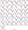 |
Fig. B.1. Continued. |
All Tables
Breakdown of the number of spectra/SNe Ia remaining after each cut to reach the final sample of 329 spectra ready for fitting.
Updated maximum light values from supplementary photometric data for improved spectral phase estimation.
All Figures
|
Fig. 1. Distributions of resolution and S/N in the 1930 spectra before the peak covering the relevant wavelength region with a clean enough signal for the S/N estimation. The bottom panel represents the redshift distribution of the 1557 objects sampled by these spectra. The dotted lines and accompanying values correspond to the medians of the three measurements. Final cuts upon S/N and resolution will be implemented based upon the results of the simulated fits. |
| In the text | |
|
Fig. 2. Palomar Transient Factory (Maguire et al. 2014) SN Ia spectral measurements for velocity, width, and depth in the case of the Si IIλ6355 absorption feature. The power law fit to the velocity evolution and the Gaussian KDE (described by the contours) for the width and depth are used to inform the generation of the synthetic features in the simulations. |
| In the text | |
|
Fig. 3. True (circles) and false (arrows) positive rates of the MCMC/BIC classification method as a function of the velocity separations derived from the simulations for increasing S/Ns (from left to right in the panels) and different spectral dispersions (shown as different colours). One-dimensional slices (in Δv space) of the 3D GP interpolation of S/N, dispersion, and velocity separation are presented as the coloured lines and associated 68% confidence interval regions. |
| In the text | |
|
Fig. 4. Distribution of the pulls (residual/uncertainty) for the six feature parameters in the case of spectra with an S/N of 15, a dispersion of 5 Å/pix, and a velocity separation of 5000 km s−1. The solid black lines indicate the desired zero pull value, while the solid coloured lines indicate the means of the distributions, the values of which are shown in the top left corner of each panel. The dotted lines display the measured standard deviations. |
| In the text | |
|
Fig. 5. Standard deviations of the pull distributions about their means for each of the simulations. The three S/Ns are represented by different colours, as indicated above the top-left panel. The thick solid lines describe the linear regression fits to the data points with each of the three dispersions. The black point in each panel presents the standard deviation of the points around this fit. We highlight that the RHVF panel has a different y-axis scaling due to the larger standard deviation values. |
| In the text | |
|
Fig. 6. Means of the pull distributions for each of the simulations after applying the uncertainty corrections. The formatting matches that of Fig 5. The thick black lines present linear regressions to these trends that can be used to characterise and then correct for the biases. The black point in each panel presents the standard deviation of the points around this fit. |
| In the text | |
|
Fig. 7. Evolution of the velocities of the PV and HV Si IIλ6355 components for all 329 spectra in the sample (top panel). The hollow points correspond to the 244 PV components with no HV counterpart. The solid blue line is fit to all the PV components, with the dash-dotted and dotted blue lines showing fits to the PV components of spectra with and without HV components, respectively. The pink line is the fit to the HV components and the grey line is the evolution from the PTF sample (Maguire et al. 2014). The width against depth for the measured PV and HV Si IIλ6355 components using the same colours as the top panel (bottom panel). The grey contours show the KDE for the PTF sample for comparison. |
| In the text | |
|
Fig. 8. Residuals between the true positive rates taken from simulated spectra with aHV ≤ 0.25 or cHV ≤ 70 Å and the original true positive rates as a function of velocity separation for the three S/Ns. |
| In the text | |
|
Fig. 9. Evolution of the component velocities (top), parameter RHVF (pEWHV/pEWPV; middle), and the separation of the PV and HV features in velocity space (bottom). The measurements for individual spectra are plotted in grey, with the coloured points and lines corresponding to SNe Ia for which we have multiple spectra. The hollow points in the top panel correspond to the HV components. The cluster of points in the middle panel at R = 0 correspond to all the spectra identified as not having an HV component. |
| In the text | |
|
Fig. 10. Top: Kolmogorov-Smirnov p-values between our base sample and the control sample for six parameters. The solid black line describes the threshold below which a parameter should be considered to show a bias when compared to the ‘low-bias’ control sample. The dotted black line indicates the final redshift cut of 0.06. Bottom: Distributions of the control sample (bars) and the final sample of 190 SNe after a redshift cut at z = 0.06 (step). The p-values from the corresponding KS-tests are denoted in each of the panels. |
| In the text | |
|
Fig. 11. Velocity separation distribution of the 64 HVF spectra from our low-bias sample of 210 SNe. The black curve presents the median spectrum density after correcting for the detection efficiency of our classification method. The individual orange curves correspond to 1000 iterations of sampling the Δv values from their individual measurement distributions, rescaling the distribution, and recalculating this density function. |
| In the text | |
|
Fig. 12. Phase histogram for the 64 HVF spectra compared to the full 210 low-bias spectral sample. The solid black curve presents the median HVF spectrum density after correcting for the detection efficiency of our classification method, with the dotted black curve as the density of the full 210 spectra. The individual green curves (dark for HVF and pale for the full sample) correspond to 1000 iterations of sampling the Δv and phase values from their individual measurement distributions, rescaling the HVF distribution, and recalculating these density functions. |
| In the text | |
|
Fig. 13. SALT2 x1 histogram for the 56 HVF SNe compared to the full 190 low-bias sample. The solid black curve presents the median HVF SN density, and the dotted black curve indicates the density of the full 210 spectra. We performed no detection efficiency scaling upon the x1 parameter distribution. The individual blue curves (dark for HVF and pale for the full sample) correspond to 1000 iterations of sampling the x1 values from their individual measurement distributions and recalculating these density functions. |
| In the text | |
|
Fig. 14. Distributions of peak ZTFg-band magnitude, Δm15 in ZTFg, host galaxy mass, and local g-r colour for the HVF and non-HVF subsets of the 190 SNe low-bias sample. The means of each distribution are displayed as the dotted lines with the KS test p-values indicated in each panel. |
| In the text | |
|
Fig. 15. Ratio of the pseudo-equivalent widths of the HV and PV components against the photospheric velocity of the Si IIλ6355 feature for the low-bias sample of 190 SNe. For objects with multiple spectra we take the mean value in both dimensions, treating the uncertainties with the ASYMMETRIC UNCERTAINTY package (Gobat 2022). The vertical dotted line indicates the 12 000 km s−1 cut velocity at maximum light between the NVW (red) and HVW (green) SNe Ia. |
| In the text | |
|
Fig. 16. Comparison of the photospheric velocity (top) and pEW (bottom) measured using the single component fits against taking into consideration the HV components and using the two component fits wherever an HV component was identified. Solid data points represent the low-bias sample, with hollow data points corresponding to the remaining objects from the full sample with z > 0.06. The points indicated in orange would be misclassified in the Wang scheme and Branch scheme in the top and bottom panels respectively, if the HV components were not to be considered. These two classification schemes concern spectra around maximum light, and as such, all the spectra presented here have phases greater that –5 d. |
| In the text | |
|
Fig. 17. Comparison of the measured velocity distributions of PV and HV components in our sample for spectra identified as having both components (top) against the distributions of silicon from a number of theoretical explosion models from the HESMA archive (Kromer et al. 2017). Each of the three panels corresponds to a different explosion mechanism, with each row of the colour plot as an individual, unique model. |
| In the text | |
|
Fig. A.1. An example of a SALT2 fit to a DR2 g-band light curve of ZTF19abjkfrf, which results in a poor spectral phase estimate due to low coverage and single-band data. The original SALT2 fit is shown in green with the updated fit to the supplementary data from ATLAS in the cyan (ATLASc) and orange (ATLASo) filters displayed by the cyan and orange curves. The spectral date is represented by the solid grey vertical line, with the dotted vertical lines corresponding to the original (green) and updated (black) maximum light fit measurements. |
| In the text | |
|
Fig. B.1. Best fits to the 85 ZTF DR2 spectra in the sample identified as having an HV component. The phase and SN ZTF name are indicated in each panel. The continuum regions are highlighted in blue and red, the overall fits are shown by the solid black curves, and the individual PV and HV components are shown by the blue and pink curves. Red SN names indicate those that were subsequently cut in the creation of the low-bias sample. |
| In the text | |
|
Fig. B.1. Continued. |
| In the text | |
Current usage metrics show cumulative count of Article Views (full-text article views including HTML views, PDF and ePub downloads, according to the available data) and Abstracts Views on Vision4Press platform.
Data correspond to usage on the plateform after 2015. The current usage metrics is available 48-96 hours after online publication and is updated daily on week days.
Initial download of the metrics may take a while.