| Issue |
A&A
Volume 698, June 2025
|
|
|---|---|---|
| Article Number | A70 | |
| Number of page(s) | 12 | |
| Section | Extragalactic astronomy | |
| DOI | https://doi.org/10.1051/0004-6361/202452864 | |
| Published online | 28 May 2025 | |
SN 2023xqm: A gradually fading Ia supernova exhibiting isolated high-velocity signatures
1
Center for Astronomy and Space Sciences, China Three Gorges University, Yichang 443000, People’s Republic of China
2
College of Mathematics and Physics, China Three Gorges University, Yichang 443000, People’s Republic of China
3
Beijing Planetarium, Beijing Academy of Science of Technology, Beijing 100044, People’s Republic of China
4
Physics Department and Tsinghua Center for Astrophysics (THCA), Tsinghua University, Beijing 100084, People’s Republic of China
5
Department of Physics, University of California, Santa Barbara, CA 93106-9530, USA
6
Las Cumbres Observatory, 6740 Cortona Drive Suite 102, Goleta, CA 93117-5575, USA
7
Xinjiang Astronomical Observatory, Chinese Academy of Sciences, Urumqi, Xinjiang 830011, People’s Republic of China
⋆ Corresponding authors: This email address is being protected from spambots. You need JavaScript enabled to view it.
, This email address is being protected from spambots. You need JavaScript enabled to view it.
Received:
4
November
2024
Accepted:
10
April
2025
Abstract
We conducted an exhaustive analysis combining optical photometry and spectroscopy of the type Ia supernova designated SN 2023xqm. Our observational period spanned from the two weeks preceding to 88 days after the B-band peak luminosity time. We determined the peak brightness in the B-band to be −18.90 ± 0.50 mag, and it is accompanied by a moderately slow decay rate of 0.90 ± 0.07 mag. The maximum quasi-bolometric luminosity was estimated to be 1.52 × 1043 erg s−1 and correlated with a calculated 56Ni mass of 0.74 ± 0.05 M⊙, aligning with the modestly reduced rate of light curve decay. A plateau that can be observed in the r − i color curve might correlate with the minor elevation noted between the principal and secondary peaks of the i-band light curve. An initial spectral analysis of SN 2023xqm revealed distinct high-velocity features (HVFs) in Ca II that contrast with the subdued HVFs observed in Si II. Such attributes may stem from variations in ionization or temperature or from scenarios involving enhanced element abundance, suggesting a naturally lower photospheric temperature for SN 2023xqm, which could be indicative of incomplete burning during the white dwarf’s detonation. The observed traits in the light curve and the spectral features offer significant insights into the variability among type Ia supernovae and their explosion dynamics.
Key words: supernovae: general / supernovae: individual: SN 2023xqm
© The Authors 2025
 Open Access article, published by EDP Sciences, under the terms of the Creative Commons Attribution License (https://creativecommons.org/licenses/by/4.0), which permits unrestricted use, distribution, and reproduction in any medium, provided the original work is properly cited.
This article is published in open access under the Subscribe to Open model. This email address is being protected from spambots. You need JavaScript enabled to view it. to support open access publication.
1. Introduction
Type Ia supernovae (SNe Ia) are widely accepted to be the result of the catastrophic detonation of carbon-oxygen-rich white dwarfs within binary star systems, where a rapid thermonuclear reaction takes place, as referenced in various studies (Hillebrandt & Niemeyer 2000; Maoz et al. 2014; Livio & Mazzali 2018; Soker 2019; Jha et al. 2019; Liu et al. 2023). Their uniform light curve profiles (e.g., Barbon et al. 1973; Elias et al. 1981) and the close relationship between their B-band peak brightness and subsequent decay rate (e.g., Phillips 1993; Jha et al. 2019) make SNe Ia the premier cosmic distance markers, and they are effective up to redshifts of approximately two (Riess et al. 1998; Perlmutter et al. 1999; Riess et al. 2016, 2018, 2022). Two theoretical models are predominantly considered for the genesis of SNe Ia: the double-degenerate (DD) scenario (Webbink 1984; Iben & Tutukov 1984; Tutukov & Yungelson 1996; Toonen et al. 2012; Ruiter et al. 2013) and the single-degenerate (SD) scenario (Whelan & Iben 1973; Marietta et al. 2000; Han & Podsiadlowski 2006; Podsiadlowski et al. 2008; Meng & Yang 2011; Justham 2011). For the DD framework, the supernova event is triggered in a binary system featuring two white dwarfs. Over time, these stars draw closer and ultimately coalesce, unleashing an immense burst of energy that precipitates the supernova (Pakmor et al. 2012; Sato et al. 2015). The SD framework involves a white dwarf and a companion star that could be in the main-sequence or giant phase. Here, the white dwarf accumulates material from its companion and increases in mass until it reaches a threshold that ignites nuclear reactions and results in an explosion (Whelan & Iben 1973; Webbink 1984; Iben & Tutukov 1984). These models are central to understanding the mechanisms behind SNe Ia despite the ongoing uncertainties and discussions (Wang et al. 2013; Maoz et al. 2014; Jha et al. 2019; Han et al. 2020). Some preliminary findings have hinted at the absence of companion stars in certain SNe Ia, which could support the DD hypothesis (Schaefer & Pagnotta 2012; Olling et al. 2015; Tucker et al. 2019). On the other hand, the possible identification of circumstellar material (CSM) around some SNe Ia suggests the SD model may be at play in at least some cases (Wang et al. 2004; Blondin et al. 2009; Silverman et al. 2013; Wang et al. 2019). However, it is important to acknowledge that theoretical research suggests CSM could also originate from the DD scenario (Shen et al. 2013; Levanon & Soker 2017).
The specific processes that lead to the ignition of SNe Ia continue to be a topic of vigorous scholarly debate and discussion (Kasen & Plewa 2005; Maoz et al. 2014; Soker 2019; Wang et al. 2024). Currently, the process of evolving from a subsonic deflagration to a supersonic detonation within a white dwarf of Chandrasekhar mass, referred to as the delayed detonation scenario, is widely adopted for modeling such catastrophic stellar events (Khokhlov 1991a,b; Seitenzahl et al. 2013; Jha et al. 2019; Liu et al. 2023). Additionally, the gravitationally confined detonation (GCD) model has been put forward by Plewa et al. (2004), Kasen & Plewa (2005), which involves an off-center ignition that spreads toward the outer layers. However, these theoretical frameworks face certain challenges, such as an excessive synthesis of 56 Ni (Wang et al. 2008) and the creation of highly polarized material, which do not align with spectropolarimetric observations from SNe Ia (with a mean polarization of ∼0.32%; Cikota et al. 2019), though Nagao et al. (2024) observed high polarization in several peculiar subtype of Ia supernovae. There is also a growing interest in models involving sub-Chandrasekhar mass white dwarfs, particularly those that consider a double-detonation sequence (Fink et al. 2007; Kromer et al. 2010; Woosley & Kasen 2011; Shen & Bildsten 2014; Shen & Moore 2014; Polin et al. 2019). A variety of alternative pathways are under investigation for their potential role in leading to SNe Ia, including catastrophic collisions between two white dwarfs (Benz et al. 1990; Pakmor et al. 2012; Shen et al. 2012), triple system interactions (Kushnir et al. 2013), detonation events in rapidly spinning white dwarfs surpassing the Chandrasekhar threshold (Di Stefano et al. 2011), and explosions initiated in the core of degenerate stars (Kashi & Soker 2011; Wang et al. 2017).
To deepen comprehension of the intrinsic physics behind SNe Ia, these cosmic phenomena have been meticulously sorted into diverse subtypes according to their detected attributes. Type Ia supernovae have a wide diversity, but most of them belong to the normal type (Graur et al. 2017; Li et al. 2023; Desai et al. 2024; Dimitriadis et al. 2025). However, a subset displays atypical traits, such as the dim 1991bg-like supernovae delineated by Filippenko et al. (1992a) and the intensely bright 1991T-like supernovae outlined by Filippenko et al. (1992b) and Ruiz-Lapuente et al. (1992). Based on unique photometric and spectral characteristics, normal type Ia supernovae have been further refined to include a number of special types of subclasses (Liu et al. 2023; Ruiter & Seitenzahl 2025). Benetti et al. (2005) categorized standard SNe Ia into high-, medium-, and low-velocity gradient groups based on the rate of change of the Si IIline’s velocity over time. Branch et al. (2006) proposed a system based on the strength of the Si IIλλ5972,6355 lines at the B-band peak, resulting in the identification of several subgroups, including core-normal, broad-line, cool, and shallow-silicon types. Wang et al. (2009a) recommended a further bifurcation of “branch-normal” SNe Ia into normal-velocity (NV; where v < 12 000 km/s) and high-velocity (HV; where v ≥ 12 000 km/s) categories based on the Si IIλ6355 line’s velocity at the B-band peak. The presence of high-velocity features (HVFs; Silverman et al. 2015; Zeng et al. 2021a; Harvey et al. 2025), which are frequently observed in the Ca II NIR triplet lines and sporadically in the Si IIλ6355 lines of certain SNe Ia, assists in subtype differentiation. SN 2023xqm, which is characterized by its gradually receding light curves and distinct HVF, provides an insightful instance for probing the genesis of SNe Ia.
This manuscript is structured as follows: In Sect. 2, we outline the methodologies for optical data collection and subsequent reduction processes. Section 3 presents an in-depth analysis of the photometric light curves, color curves, and the synthesis of the quasi-bolometric light curve. Subsequently, in Sect. 4, we analyze the spectral time-domain evolution of the supernova. In Sect. 5 we explore the nuances of the light curve, the distribution of intermediate-mass elements, and the potential detonation dynamics of SN 2023xqm. The paper concludes with Sect. 6, where we synthesize the findings.
2. Data acquisition
The supernova designated as SN 2023xqm was first identified on November 13, 2023, at the celestial coordinates  , δ = − 27° 39′03″.31 (J2000) by the ATLAS survey (Tonry et al. 2023). It exploded at the edge of the host galaxy NGC 3285B, which has a redshift of 0.009847 ± 0.000033 (Kaldare et al. 2003). This survey initially recorded the supernova at a magnitude of c = 17.885 in the AB magnitude system, as reported by Tonry et al. (2023). A series of multi-band photometry was performed on SN 2023xqm utilizing a series of telescopes, among which were the facilities of the Las Cumbres Observatory (LCO) and the Asteroid Terrestrial-impact Last Alert System (ATLAS), as detailed in Brown et al. (2013), Tonry et al. (2018), and Smith et al. (2020). The LCO’s Global Supernova Project conducted an extensive campaign of photometric observations on SN 2023xqm, covering the UBVgri bands with measurements collected on an approximately daily basis from 14 days prior to 88 days post the B-band peak. Figure 1 displays an image captured by LCO. The observational data of SN 2023xqm were processed using AutoPhot (Brennan & Fraser 2022), and the multi-band photometry was calibrated against the Gaia synthetic photometry catalog (Gaia Collaboration 2023). Further details on the standards and observations are outlined in Tables 1 and 2, respectively. Furthermore, a set of 14 low-resolution optical spectra for SN 2023xqm was obtained through the FLOYDS spectrographs mounted on the Faulkes Telescopes, which are components of the LCO’s Global Supernova Program (Sand et al. 2011; Brown et al. 2013; Howell & Global Supernova Project 2017). We sourced an additional spectrum observed by the European Southern Observatory’s New Technology Telescope (Kopsacheili et al. 2023) from theTransient Name Server(TNS). Standard spectral processing was carried out using IRAF routines (Tody et al. 1986) and followed by calibration of SN 2023xqm’s spectral flux through comparison with standard stars observed under similar conditions on the same night (Fig. 2).
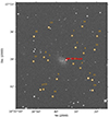 |
Fig. 1. Typical observation of SN 2023xqm by the LCO network. SN 2023xqm is marked with a red circle, while the photometric standard stars are indicated by orange circles. |
Photometric standards used in the SN 2023xqm field.
Optical photometric observations of SN 2023xqm.
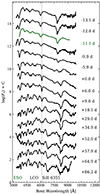 |
Fig. 2. Progression of the optical spectrum for SN 2023xqm. Each spectrum has undergone de-reddening based on the host galaxy’s characteristics and redshift data. The time indicators on the spectra’s right-hand side denote the days elapsed since the B-band’s peak luminosity. The vertical dashed lines pinpoint the absorption troughs of the Si II 6355 feature in SN 2023xqm’s spectrum, observed around t ∼ +0.0 days. |
3. Light curves
3.1. Time domain observations
Figure 3 presents a comparative examination of the UBVgri-band light curves of SN 2023xqm alongside those of several other SNe Ia with analogous traits, including SNe 2005cf (Garavini et al. 2007; Pastorello et al. 2007; Wang et al. 2009b; Gall et al. 2012), 2011fe (Richmond & Smith 2012; Pereira et al. 2013; Munari et al. 2013; Kerzendorf et al. 2014; Zhang et al. 2016; Milne et al. 2017; Friesen et al. 2017; Dimitriadis et al. 2017; Kerzendorf et al. 2017; Mulligan & Wheeler 2018; DerKacy et al. 2020; Tucker et al. 2022a,b; Tucker & Shappee 2024), 2017hpa (Zeng et al. 2021b; Dutta et al. 2021), 2017erp (Jha et al. 2017; Fung et al. 2019; Brown et al. 2019), 2018oh (Li et al. 2019; Levanon & Soker 2019; Dimitriadis et al. 2019), 2021hpr (Zhang et al. 2022; Barna et al. 2023; Lim et al. 2023, 2024), and 2023wrk (Liu et al. 2024; Andrade et al. 2024). Each light curve is in the rest-frame and has been K-corrected using SNooPy2 (Burns et al. 2011, 2014), and then scaled to their respective peak magnitudes. The B-band light curve of SN 2023xqm aligns closely with the general form observed in other typical SNe Ia in the phase leading up to the peak. Its rate of decline and intrinsic brightness closely mirror those of SN 2018oh (Li et al. 2019). However, the i-band light curve of SN 2023xqm shows a marginally more pronounced secondary peak compared to its counterparts. Although more luminous, the rate of decline for SN 2023xqm is less than that of SN 2011fe, which has a typical value of 1.103 ± 0.035 mag. SN 2023xqm also demonstrates a comparatively elevated luminosity relative to other SNe Ia at analogous stages. Collectively, the light curve progression of SN 2023xqm adheres to the general pattern observed in other standard SNe Ia.
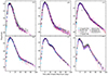 |
Fig. 3. Comparative analysis of the optical light curves (in the UBVgri bands) of SN 2023xqm with several well-observed SNe Ia. The light curves of the compared SNe Ia have been scaled to align with the peak magnitudes of SN 2023xqm. |
The updated Hubble constant (H0 = 72.3 ± 2.8 km s−1 Mpc−1) was utilized to calculate the distance (Galbany et al. 2023). We used the EBV_model2 in SNooPy2 to analyze the multiband light curves of SN 2023xqm, which resulted in an estimated B-band peak magnitude of 14.71 ± 0.02 mag at MJD 60 276.65 ± 0.20. The B-band decline rate after the peak, Δm15(B), was measured to be 0.90 ± 0.07 mag, and the color stretch, represented by sBV, was determined to be 1.06 ± 0.07 . The corresponding parameters are displayed in Table 3.
Basic parameters measured for SN 2023xqm.
Figure 5 displays the optical color evolution of SN 2023xqm contrasted with the color evolutions of several other meticulously tracked supernovae: SN 2005cf, SN 2011fe, SN 2017hpa, SN 2018oh, SN 2021hpr, and SN 2023wrk. Compared to other supernovae, the color profile of SN 2023xqm shows a relatively reddish color profile evolution pathway before reaching its bluest color peak. Regarding the B − V and g − r color evolutions, SN 2023xqm attains its most bluish tint around t ≈ − 6 days and then gradually turns red, reaching its most reddish point around t ≈ + 32 days. The B − V color evolution of SN 2023xqm closely mirrors that of SN 2005cf. As depicted in Figure 5, for the r − i color evolution of SN 2023xqm, after peaking in brightness, there is a brief plateau phase at approximately −0.7 mag that is followed by a swift reddening trend until it reaches approximately −0.1 mag around t ≈ + 35 days. After this point, the color evolution gradually shifts toward the bluer end. This plateau may be linked to a minor peak in the r-band light curve post-maximum. The g − i color evolution of SN 2023xqm experiences minor oscillations near its bluest peak. The most bluish g − i color, at approximately −0.8 mag, occurs around t ≈ + 14 days, while the most reddish g − i color, at approximately 1.0 mag, is observed around t ≈ + 35 days. Additionally, when contrasted with other supernovae, the g − r and g − i color trajectories of SN 2023xqm are marginally redder.
3.2. Quasi-bolometric light curve
The application of the SNooPy2 fitting to the light curves of SN 2023xqm in different filters yielded a mean distance modulus of μ = 33.85 ± 0.05 mag (see Figure 4). According to Tully et al. (2013), the distance modulus for the host galaxy NGC 3285B is estimated to be 32.98 ± 0.47 mag. As SN 2023qxm is not in the Hubble flow, the better estimate is the redshift-independent distance (32.98 ± 0.47 mag), which we used for subsequent analyses. After applying extinction corrections for both the galactic and the host galaxy and assuming RV = 3.1, we found the estimated absolute peak magnitude in the B-band for SN 2023xqm is Mmax(B) = −18.90 ± 0.50 mag. The brightness of SN 2023xqm is relatively low compared to typical values (Phillips 1993), and the significant uncertainty in its brightness is primarily due to the uncertainty in the distance estimation.
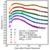 |
Fig. 4. Optimal light curve model for SN 2023xqm derived from SNooPy2 (solid black lines). The dashed black lines indicate the 1σ variability, which corresponds to the precision of the light curve patterns. The height of the curves has been adjusted to enhance visual distinction. |
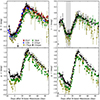 |
Fig. 5. Color curves of B − V, r − i, g − r, and g − i of SN 2023xqm compared to those of SNe 2005cf, 2011fe, 2017hpa, 2018oh, 2021hpr, and 2023wrk. All the color curves have been corrected for reddening using SNooPy2. The shaded gray area indicates the bump after the maximum in the i-band light curve. |
We synthesized the synthetic bolometric light curve representing SN 2023xqm by integrating the optical photometry spectral energy distribution (SED) across multiple bands, encompassing the UBVgri filters, as referenced in Li et al. (2019). In constructing this curve, it was presupposed that the near-infrared (NIR) and ultraviolet (UV) emissions of SN 2023xqm have a comparable impact, aligning with the observations from SN 2011fe (Zhang et al. 2016). Figure 6 presents a comparative analysis of the light curves of SN 2023xqm with those of SN 2005cf (Pastorello et al. 2007; Wang et al. 2009b) and SN 2011fe (Zhang et al. 2016). A close examination of the figure reveals that the initial phase development of SN 2023xqm’s quasi-bolometric light curve is strikingly similar to SN 2005cf. The luminosity of SN 2023xqm peaked at Lpeak ∼ 1.52 × 1043 erg s−1, which exceeds that of SN 2011fe (∼ 1.13 × 1043 erg s−1; Zhang et al. 2016) but falls short of that of SN 2005cf (∼ 1.56 × 1043 erg s−1; Wang et al. 2009b).
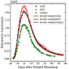 |
Fig. 6. Quasi-bolometric light curve of SN 2023xqm, which is compared with those of SN 2005cf and SN 2011fe. |
We applied the Minim Code (Chatzopoulos et al. 2012, 2013), which is grounded in the radiation diffusion framework originating from the Arnett law (Arnett 1982; Li et al. 2019; Zeng et al. 2021b), was applied to deduce the mass of nickel-56 and several related parameters. The parameters for SN 2023xqm, as described by Chatzopoulos et al. (2012), are as follows: the initial illumination time is t0 = -16.87 ± 0.03 days, the temporal extent of the light curve is tlc = 14.97 ± 0.01 days, and the duration scale for gamma-ray emissions is tγ = 33.68 ± 0.75 days. The calculated mass of synthesized 56Ni was estimated as 0.74 ± 0.05 M⊙. The relatively high 56Ni in the ejecta suggests that SN 2023xqm could have originated from a white dwarf with a mass close to the Chandrasekhar limit. As introduced by Arnett (1982), the quantity of mass in ejected material is approximated at Mej = 0.97 ± 0.04 M⊙, with the kinetic energy quantified at Ekin = (0.96 ± 0.10) × 1051 erg s−1. The same method was applied to derive the parameters of SNe 2005cf and 2011fe, which are listed in Table 4. The measured 56Ni mass of SN 2023xqm is moderate, indicating a normally bright SN Ia, which could be consistent with the Chandrasekhar mass model (Wang et al. 2008; Vallely et al. 2020). The light curve of SN 2023xqm is expected to be broad and decline slowly, suggesting that the supernova may have exploded within the delayed detonation scenario in a younger stellar environment (Wang et al. 2008; Deckers et al. 2022).
Measured parameters of SNe 2005cf,2011fe and 2023xqm.
4. Spectral observational features
4.1. Spectra compare
Figure 7 presents a side-by-side evaluation of the spectral data of SN 2023xqm against other SNe Ia with analogous Δm15(B) at four distinct temporal milestones: approximately −13, −6, 0, and 18 days relative to the B-band peak brightness. Panel(a) of Figure 7 depicts the early spectral analysis (around −13 days prior to the maximum brightness in the B-band light curve) of SN 2023xqm. At this stage, the predominant spectral traits of SN 2023xqm are largely similar to those of the other referenced SNe Ia. With the exception of SN 2021hpr, the majority of the supernovae display significant absorption lines for Ca II H&K and Si IIλ4130. The combined spectral features of Fe II and Mg IIas well as those in the vicinity of 4800 Å are nearly indistinguishable between SN 2023xqm and SN 2021hpr, and they stand out more than in the other supernovae. In this early phase, the Ca II NIR triplet is markedly visible in SN 2021hpr, SN 2005cf, and SN 2023xqm, whereas it is comparatively subdued in SN 2011fe and SN 2017hpa.
 |
Fig. 7. Spectra of SN 2023xqm were obtained at t ≈ −13, −6, +0, and +18 d relative to the B-band maximum light. These spectra were compared with the corresponding phase spectra of other supernovae, including SN 2011fe (Zhang et al. 2016), SN 2017hpa (Zeng et al. 2021b), SN 2021hpr (Zhang et al. 2022), and SN 2005cf (Wang et al. 2009b). |
Around one week prior to the peak brightness in the B-band, SN 2023xqm exhibited a growing resemblance to the comparative SNe Ia (see Figure 7b). During this phase, the spectral data of SN 2023xqm began to display the W-shaped absorption features of S II and Si IIλ5972 along with a noticeable absorption line corresponding to Si IIλ4130. When comparing the Ca II NIR triplet among the supernovae, noticeable differences persisted, particularly in the relative strengths of the HVFs and photospheric components. At the B-band maximum light phase, the spectrum of SN 2023xqm closely resembles those of the compared SNe Ia, as illustrated in Figure 7c. We determined the line strength ratio R(Si II) (Nugent et al. 1995), which is defined as the equivalent width (EW) ratio between Si IIλ5972 and Si IIλ6355 in the spectrum at the vicinity of peak luminosity, to be 0.05 ± 0.01 for SN 2023xqm. Compared to the typical measurement of R(Si II) = 0.28 ± 0.04 for normal SN 2005cf (Wang et al. 2009b) and 0.085 ± 0.006 for SN 2021hpr, the lower R(Si II) measured for SN 2023xqm indicates that it may have a relatively higher photospheric temperature (Nugent et al. 1995). At t ≈ + 18 d, it is evident from the comparative spectra of supernovae (see Figure 7d) that the spectral features are dominated by lines of Ca II, Si II and iron-group elements, including the Ca II NIR triplet, which shows considerable diversity from that in the early phase. The distinctive W-shaped profile of the S II line is nearly absent in SN 2023xqm and the comparison sample. The absorption line of Ca II NIR remains prominent in the spectra and experiences a resurgence in strength.
With the photosphere receding, the Si IIλ6355 absorption feature shifts gradually toward the red end. Figure 7 illustrates that at approximately t ≈ − 13 d, the Si IIλ6355 absorption line in the spectra of SN 2023xqm appears to be blue-ward compared to SN 2011fe, SN 2017hpa, and SN 2005cf. However, by t ≈ − 6 d, the Si IIλ6355 absorption profile of SN 2023xqm aligns almost perfectly with those of other supernovae. This suggests that SN 2023xqm could experience a faster early-phase velocity decline compared to other supernovae. Moreover, the absorption line of O Iλ7774 in the spectra of SN 2023xqm is not prominent, which suggests that the oxygen element in SN 2023xqm has undergone relatively thorough burning (Zhao et al. 2016).
4.2. Velocity evolutions
Figure 8 illustrates the velocity evolution of the ejected material for SN 2023xqm derived from the Gaussian-fitting minimum of the Si IIλ6355 absorption profile in observed spectra. This velocity profile has been compared with other extensively observed supernovae, including SN 1991T-like (Matheson et al. 2008), 1991bg-like (Wang et al. 2009a; Silverman 2011), SNe 2005cf, and 2011fe. Following the categorization framework proposed by Wang et al. (2009a), SN 2023xqm could be identified as a member of the NV subclass of SNe Ia based on the B-band maximum light velocity of 10580 ± 290 km s−1 derived from the Si IIλ6355 line profile. The velocity gradient of SN 2023xqm, calculated as  = 54.8 ± 13.7 km s−1 d−1, places it within the low-velocity gradient subtype in the classification developed by Benetti et al. (2005). During its early stages, SN 2023xqm exhibited an expansion velocity approximately 3000 km s−1higher than of SN 2012fr, SN 2005cf, and SN 2011fe. The expansion velocity decreased rapidly until 10 days before B-band maximum light and gradually slowed down around the time of the B-band maximum light. This may indicate the existence of HVFs in the Si IIλ6355 absorption line.
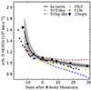 |
Fig. 8. Progression of velocities for the Si IIλ6355 line in SN 2023xqm analyzed in relation to other supernovae, including SN 2005cf and SN 2011fe (see text for the references). The velocity evolution profiles for supernovae akin to SN 1991T and SN 1991bg are illustrated with dashed red and blue lines, respectively, with velocity assessments made at the absorption line’s lowest point of Si IIλ6355. The shaded area represents the 1σ uncertainty surrounding the average velocity evolution for high-velocity SNe Ia according to Wang et al. (2009a). Comparative supernova data and the zone indicating typical SNe Ia are derived from Li et al. (2019). |
5. Discussion
5.1. Light curve feature and modeling
As presented in Figure 6, the r − i color curve of SN 2023xqm shows a short plateau stage during ∼3 days to ∼17 days with respect to the B-band maximum brightness. According to Kasen (2006), as the ionization state transitions from double to single, the gas enriched with iron exhibits intense luminescence, efficiently shifting the ubiquitous blue light toward the red end of the spectrum. The second peak observed in the near-infrared (NIR) bands of SN 2023xqm may be attributed to the energy released as iron elements in the core region recombine from a doubly ionized state to a singly ionized state. Similarly, the small bump just after the maximum light in the i-band light curve could be attributed to the recombination from triply to doubly ionized states in supernova ejecta (Kasen 2006).
As Magee et al. (2020) notes, disparities in density gradients result in varied 56 Ni distributions across velocity spaces within supernova ejecta. Models characterized by elevated kinetic energies tend to distribute a larger quantity of 56 Ni to higher velocity regions, leading to enhanced early luminosity. In Figure 9, we have adopted the explosion models from Magee et al. (2018, 2020) in order to perform a comparison of the light curves of SN 2023xqm. The model light curves were calculated using the radiative transfer code TURTLS1 (Magee et al. 2018), which is a one-dimensional Monte Carlo radiation transfer program. The code is used to simulate the early (near maximum) light curve of thermonuclear supernovae. The input structure (density, composition, and speed range) of SN ejecta is freely defined by the user, and the Monte Carlo packages are utilized to track the radioactive decay of 56 Ni and subsequent 56 Co. The models with double power law (DPL) and exponential (EXP) density profiles (Magee et al. 2020) were employed to compare the observed multi-band light curves of SN 2023xqm. The best-fitting models are DPL_Ni0.4_KE1.68_P4.4 and EXP_Ni0.6_KE0.78_P4.4, as shown in Figure 9. It is evident that SN 2023xqm exhibits a better match with the EXP_Ni0.6_KE0.78_P4.4 model, as it demonstrates a closer agreement in the comparison. Magee et al. (2018) have suggested that extended models (e.g., s3) exhibit very different light curves from compact models (e.g., s9.7 and s100). The favored model has a set of parameters, 0.6 M⊙ of 56 Ni; low kinetic energies (0.78); and extended 56 Ni distributions (4.4), which suggests that a more diffuse or spread-out distribution of 56 Ni exists in the ejecta of SN 2023xqm. This also indirectly suggests that the early ejecta of SN 2023xqm could have been mixed with a certain mass of iron-group elements, and the existence of these elements in the early ejecta is related to the small bump in the i-band light curve after the maximum light.
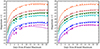 |
Fig. 9. Comparison of the light curves of SN 2023xqm with the TURTLS models (Magee et al. 2020). The left panel shows the best-fitting model of DPL density profile of DPL_Ni0.4_KE1.68_P4.4. The right panel depicts the best-fitting model with EXP density profile of EXP_Ni0.6_KE0.78_P4.4. |
As we illustrate in Figure 10, the light curves of SN 2023xqm were fit using the combined companion-shocking and SiFTO template as described in the works of Burke et al. (2021) and Hosseinzadeh et al. (2023). The fitting process was performed using the released lightcurve_fitting package (Hosseinzadeh et al. 2024), which involves several parameters: (1) the parameter representing the time of explosion, denoted as t0; (2) the parameter representing the separation of the binary system in the companion-shocking interaction, denoted as a; (3) the parameter θ, which is essential for the geometric interpretation of the light curve, as it represents the viewing angle (Brown et al. 2012); (4) the parameter tmax(B), which refers to the B-band maximum specifically for the SiFTO template; (5) the parameter s, which denotes the expansion factor employed with the SiFTO template; (6) the parameter ΔtU, which denotes the shift factor applied to the peak time of U-band light curve; (7) the parameter Δti, which represents the shift factor applied to the i-band maximum light time; (8) the parameter σ, which is a scaling factor that adjusts the data errors to account for possible underestimation. Table 5 provides a comprehensive description of the initial and best-fit values for these parameters. The B-band maximum time, tmax(B), determined by the model exhibits a close agreement with the estimation obtained from SNooPy2, so we adopted the value of MJD 60276.65 ± 0.20 of B-band maximum light in the following analysis. The rise time of SN 2023xqm could be measured as 18.2 ± 0.9 d. According to Figure 10, there is no significant difference between the “normal” type Ia component of the model fitting result (dashed line) and the combined companion-shocking and template model fitting result (solid line). The best-fit binary separation is a = 5.7 R⊙. Assuming the companion is in Roche lobe overflow (a/R ∼ 2 − 3; Kasen 2010), this value suggests a companion radius of R ∼ 1.9 R⊙. Since the radius and other values are degenerate with the viewing angle, which may not be fully accounted for here, the order of magnitude suggests a more commonly observed main-sequence or subgiant companion with a mass of 1–3 M⊙ (Kasen 2010; Hosseinzadeh et al. 2022).
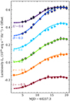 |
Fig. 10. Analysis outcomes for the initial multiband (UBVgri) luminosity profiles of SN 2023xqm. The light curves are compared with the model proposed by Kasen (2010), which takes into account the dynamic exchange between the supernova’s expelled materials and its nondegenerate companion star within a binary system. Dashed lines in the plots represent the “normal” type Ia component of the model, specifically the SiFTO template proposed by Conley et al. (2008). Solid lines depict the combined companion-shocking and SiFTO template model. Observed values are indicated by dots on the plot. The x-axis indicates the temporal progression in relation to the detonation, while the y-axis corresponds to the emitted light intensity. |
Measured parameters of the CompanionShocking3 model for SN 2023xqm.
5.2. Origin of HVFs
Measurement of the ejecta velocities from absorption lines, such as Si IIλ5972, Si IIλ6355, and the Ca II NIR triplet, was performed using the multi-Gaussian fitting method described by Zhao et al. (2015, 2016). The results are presented in Figure 11. The early time photospheric velocity, as determined from Si IIλ6355 at t ≈ −13 d, is approximately 16 390 km s−1, which is similar to the velocities observed in the Ca II NIR photospheric-velocity feature (PVF) line (approximately 16 400 km s−1). However, it is considerably slower than the velocity of the HVF estimated from the Ca II NIR HVF, which is approximately 29 400 km s−1. At the B-band maximum light, we determined the velocity of Si IIλ6355 to be 10580 ± 290 km s−1, which is lower than the typical value of approximately 11 800 km s−1observed in the NV SNe Ia (Wang et al. 2009a). Thus, SN 2023xqm could be safely categorized into the NV subclass.
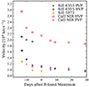 |
Fig. 11. Velocity evolution of several intermediate-mass elements that are measured from the minimum of the spectra absorption lines. The detached HVF and the PVF of Ca II and Si II are displayed for comparison. |
Figure 11 illustrates the velocity evolution of certain intermediate-mass elements in ejecta of SN 2023xqm, namely Si II and Ca II. Si IIλ5972 and the photospheric component of the Ca II NIR triplet demonstrate comparable velocity evolution patterns. However, the HVFs measured from the Si IIλ6355 and Ca II NIR triplet show higher velocities that are approximately 9000 km s−1 faster than those of PVF. Several widely accepted explanations have been proposed to account for the formation of HVFs in SNe Ia ejecta. These include the abundance enhancement scenario (Mazzali et al. 2005a,b; Maeda et al. 2010; Childress et al. 2013, 2014; Maguire et al. 2014; Silverman et al. 2015), the density enhancement scenario (Mazzali et al. 2005a,b; Tanaka et al. 2006, 2008; Townsley et al. 2012; Childress et al. 2013, 2014; Maguire et al. 2014; Silverman et al. 2015), and the ionization effect scenario (Mazzali et al. 2005a; Tanaka et al. 2008).
According to Zhao et al. (2015), the noticeable pattern of detecting high-velocity features more often in the Ca II line than in the Si II line (demonstrated by the greater pseudo-equivalent widths) observed in Ca-HVFs, as opposed to Si-HVFs, and the higher velocity formation of Ca-HVFs relative to Si-HVFs can be linked to the variation in the excitation energies required for the emission of the Si IIλ6355 line versus the Ca II IR triplet. Due to the relatively low temperatures anticipated in the outermost layer where HVFs form, the formation and saturation of Ca II IR absorption are facilitated (Childress et al. 2013; Zhao et al. 2015). This tendency is expected to become more pronounced as the velocity increases.
While the precise origin and formation mechanisms of HVFs observed in Si IIλ6355 absorption profiles remain elusive, the seminal study of Harvey et al. (2025) establishes compelling evidence for the ubiquitous presence of intermediate-mass elements in the outer ejecta of most SNe Ia. Based on the Heidelberg Supernova Model Archive (Kromer et al. 2017), Harvey et al. (2025) presents that pure subsonic burning struggles to produce the observed HVFs in SNe Ia spectra, while delayed detonation and double-detonation models can generate HVFs through stratified ejecta structures. Their formation mechanisms primarily depend on ionization profiles controlled by plasma density and abundance stratification, which require further focused investigation. Mazzali et al. (2005a) proposed that HVFs may originate from either the sweeping up of CSM produced by a companion star’s wind or three-dimensional density fluctuations (Mazzali et al. 2005a,b). These multidimensional origins are supported by the polarization differences observed in SN 2001el (Wang et al. 2003; Kasen et al. 2003)and SN 2019ein (Patra et al. 2022).
The HVFs are also believed to arise from a dense shell located at considerable distances from the center in the density enhancement scenario. The elemental makeup of this particular zone displays properties commonly associated with the carbon-oxygen enriched layer found within the outwardly expanding material (Childress et al. 2014; Maguire et al. 2014; Zhao et al. 2015). The formation of this shell is likely a result of the interaction between the ejecta from the SN and the CSM, as suggested by studies conducted by Gerardy et al. (2004), Mazzali et al. (2005b), Tanaka et al. (2006, 2008), and Mulligan & Wheeler (2018). Such a scenario can occur when the WDs undergo an explosion with a relatively dense CSM enveloped, which could be linked to the activity of the WDs before the explosion or the explosion process itself (Hoeflich et al. 1995, 1996). Alternatively, through recombination processes, the presence of these free electrons effectively reduces the ionization levels of calcium and silicon in the ionization effect scenario. As a result, a higher abundance of Ca II and Si II would be observed, which has the potential to generate HVFs (Mazzali et al. 2005a; Tanaka et al. 2008). The small bump observed in the i-band light curve of SN 2023xqm, which could be caused by the process of recombination from triply to doubly ionized states (Kasen 2006), suggests that the HVFs may be a result of an ionization effect of the ejecta.
6. Conclusion
This study provides comprehensive observations of the SN Ia 2023xqm, including extensive optical photometry and spectroscopy. The supernova was discovered in the galaxy NGC 3258B. The maximum quasi-bolometric luminosity determined from the optical light curves is estimated to be 1.52 × 1043 erg s−1, while the calculated  is 0.74 ± 0.05 M⊙. SN 2023xqm is a normal SN Ia, with a light curve decline estimated as Δm15(B) = 0.90 ± 0.07 mag. The maximum light absolute B-band magnitude is estimated as Mmax(B) = −18.90 ± 0.50 mag, while the photospheric expansion velocity at the same phase is estimated as v0 = 10580 ± 290 km s−1, which further confirms its classification as a typical SN Ia.
Overall, the evolutionary trend of SN 2023xqm is similar to that of the several supernovae we compared it to, although some differences exist in the local regions of color evolution, which may be attributed to the combined effects of differences in progenitor systems and explosion mechanisms. The small bump right after the maximum peak in the i-band light curve and the plateau in the r − i color curve together suggest the relatively low peak brightness of SN 2023xqm, which may recall that the observed characters could have arisen from ionization effects of the supernova ejecta (Kasen 2006; Tanaka et al. 2008). The spectral evolution of SN 2023xqm exhibits similarities to those of SN 2021hpr and SN 2005cf. We determined the line strength ratio R(Si II) (Nugent et al. 1995) to be 0.05 ± 0.01 for SN 2023xqm. Compared to the typical measurement of R(Si II) = 0.28 ± 0.04 for normal SN 2005cf (Wang et al. 2009b), SN 2023xqm could have a relatively higher photospheric temperature. The relatively modest light curve decline, higher luminosities, and photospheric temperatures of SN 2023xqm suggest the formation of HVFs through ionization and excitation effects.
The time domain observations of SN 2023xqm could enhance understanding of SNe Ia and their explosion mechanisms. It can also contribute to further research on SNe Ia. Additional late-time observations and investigations are necessary to determine the precise nature of SN 2023xqm.
Data availability
Full Tables 1 and 2 are available at the CDS via anonymous ftp to cdsarc.cds.unistra.fr (130.79.128.5) or via https://cdsarc.cds.unistra.fr/viz-bin/cat/J/A+A/698/A70
Acknowledgments
This research is sponsored by Natural Science Foundation of Xinjiang Uygur Autonomous Region under No. 2024D01D32 and National Natural Science Foundation of China 12203029 and U2031202, and Tian-shan Talent Training Program No. 2023TSYCLJ0053. Furthermore, this work is supported by the High Level Talent–Heaven Lake Program of Xinjiang Uygur Autonomous Region of China. Xiaofeng Wang is supported by the National Natural Science Foundation of China (NSFC grants 12288102 and 12033003), and the Tencent Xplorer prize. Xin Li is supported by the InnovationProject of Beijing Academy of Science and Technology(24CD013). The authors express their gratitude to the staffs of LCO network 1-m/2-m telescopes for supplying the data. Additionally, the LCO group receives support from NSF grants AST-1911225 and AST-1911151, as well as NASA grant Section 80NSSC19K1639. Moreover, this work has made use of data from the Asteroid Terrestrial-impact Last Alert System (ATLAS) project. The Asteroid Terrestrial-impact Last Alert System (ATLAS) project is primarily funded to search for near earth asteroids through NASA grants NN12AR55G, 80NSSC18K0284, and 80NSSC18K1575; byproducts of the NEO search include images and catalogs from the survey area. The ATLAS science products have been made possible through the contributions of the University of Hawaii Institute for Astronomy, the Queen’s University Belfast, the Space Telescope Science Institute, the South African Astronomical Observatory, and The Millennium Institute of Astrophysics (MAS), Chile. The authors thank Jialian Liu for his comments and suggestions during the writing of the manuscript.
References
- Andrade, C., Duverne, P.-A., Liu, J., et al. 2024, Res. Notes Am. Astron. Soc., 8, 273 [Google Scholar]
- Arnett, W. D. 1982, ApJ, 253, 785 [Google Scholar]
- Barbon, R., Ciatti, F., & Rosino, L. 1973, A&A, 25, 241 [Google Scholar]
- Barna, B., Nagy, A. P., Bora, Z., et al. 2023, A&A, 677, A183 [NASA ADS] [CrossRef] [EDP Sciences] [Google Scholar]
- Benetti, S., Cappellaro, E., Mazzali, P. A., et al. 2005, ApJ, 623, 1011 [NASA ADS] [CrossRef] [Google Scholar]
- Benz, W., Bowers, R. L., Cameron, A. G. W., & Press, W. H. 1990, ApJ, 348, 647 [Google Scholar]
- Blondin, S., Prieto, J. L., Patat, F., et al. 2009, ApJ, 693, 207 [CrossRef] [Google Scholar]
- Branch, D., Dang, L. C., Hall, N., et al. 2006, PASP, 118, 560 [NASA ADS] [CrossRef] [Google Scholar]
- Brennan, S. J., & Fraser, M. 2022, A&A, 667, A62 [NASA ADS] [CrossRef] [EDP Sciences] [Google Scholar]
- Brown, P. J., Dawson, K. S., Harris, D. W., et al. 2012, ApJ, 749, 18 [NASA ADS] [CrossRef] [Google Scholar]
- Brown, T. M., Baliber, N., Bianco, F. B., et al. 2013, PASP, 125, 1031 [Google Scholar]
- Brown, P. J., Hosseinzadeh, G., Jha, S. W., et al. 2019, ApJ, 877, 152 [Google Scholar]
- Burke, J., Howell, D. A., Sarbadhicary, S. K., et al. 2021, ApJ, 919, 142 [NASA ADS] [CrossRef] [Google Scholar]
- Burns, C. R., Stritzinger, M., Phillips, M. M., et al. 2011, AJ, 141, 19 [Google Scholar]
- Burns, C. R., Stritzinger, M., Phillips, M. M., et al. 2014, ApJ, 789, 32 [Google Scholar]
- Chatzopoulos, E., Wheeler, J. C., & Vinko, J. 2012, ApJ, 746, 121 [Google Scholar]
- Chatzopoulos, E., Wheeler, J. C., Vinko, J., Horvath, Z. L., & Nagy, A. 2013, ApJ, 773, 76 [NASA ADS] [CrossRef] [Google Scholar]
- Childress, M. J., Scalzo, R. A., Sim, S. A., et al. 2013, ApJ, 770, 29 [NASA ADS] [CrossRef] [Google Scholar]
- Childress, M. J., Filippenko, A. V., Ganeshalingam, M., & Schmidt, B. P. 2014, MNRAS, 437, 338 [CrossRef] [Google Scholar]
- Cikota, A., Patat, F., Wang, L., et al. 2019, MNRAS, 490, 578 [NASA ADS] [CrossRef] [Google Scholar]
- Conley, A., Sullivan, M., Hsiao, E. Y., et al. 2008, ApJ, 681, 482 [NASA ADS] [CrossRef] [Google Scholar]
- Deckers, M., Maguire, K., Magee, M. R., et al. 2022, MNRAS, 512, 1317 [NASA ADS] [CrossRef] [Google Scholar]
- DerKacy, J. M., Baron, E., Branch, D., et al. 2020, ApJ, 901, 86 [Google Scholar]
- Desai, D. D., Kochanek, C. S., Shappee, B. J., et al. 2024, MNRAS, 530, 5016 [NASA ADS] [CrossRef] [Google Scholar]
- Dimitriadis, G., Sullivan, M., Kerzendorf, W., et al. 2017, MNRAS, 468, 3798 [NASA ADS] [CrossRef] [Google Scholar]
- Dimitriadis, G., Foley, R. J., Rest, A., et al. 2019, ApJ, 870, L1 [NASA ADS] [CrossRef] [Google Scholar]
- Dimitriadis, G., Burgaz, U., Deckers, M., et al. 2025, A&A, 694, A10 [NASA ADS] [CrossRef] [EDP Sciences] [Google Scholar]
- Di Stefano, R., Voss, R., & Claeys, J. S. W. 2011, ApJ, 738, L1 [Google Scholar]
- Dutta, A., Singh, A., Anupama, G. C., Sahu, D. K., & Kumar, B. 2021, MNRAS, 503, 896 [Google Scholar]
- Elias, J. H., Frogel, J. A., Hackwell, J. A., & Persson, S. E. 1981, ApJ, 251, L13 [NASA ADS] [CrossRef] [Google Scholar]
- Filippenko, A. V., Richmond, M. W., Matheson, T., et al. 1992a, ApJ, 384, L15 [CrossRef] [Google Scholar]
- Filippenko, A. V., Richmond, M. W., Branch, D., et al. 1992b, AJ, 104, 1543 [NASA ADS] [CrossRef] [Google Scholar]
- Fink, M., Hillebrandt, W., & Röpke, F. K. 2007, A&A, 476, 1133 [NASA ADS] [CrossRef] [EDP Sciences] [Google Scholar]
- Friesen, B., Baron, E., Parrent, J. T., et al. 2017, MNRAS, 467, 2392 [NASA ADS] [Google Scholar]
- Fung, J., Zhu, Z., & Chiang, E. 2019, ApJ, 887, 152 [NASA ADS] [CrossRef] [Google Scholar]
- Gaia Collaboration (Montegriffo, P., et al.) 2023, A&A, 674, A33 [CrossRef] [EDP Sciences] [Google Scholar]
- Galbany, L., de Jaeger, T., Riess, A. G., et al. 2023, A&A, 679, A95 [NASA ADS] [CrossRef] [EDP Sciences] [Google Scholar]
- Gall, E. E. E., Taubenberger, S., Kromer, M., et al. 2012, MNRAS, 427, 994 [NASA ADS] [CrossRef] [Google Scholar]
- Garavini, G., Nobili, S., Taubenberger, S., et al. 2007, A&A, 471, 527 [NASA ADS] [CrossRef] [EDP Sciences] [Google Scholar]
- Gerardy, C. L., Höflich, P., Fesen, R. A., et al. 2004, ApJ, 607, 391 [Google Scholar]
- Graur, O., Bianco, F. B., Modjaz, M., et al. 2017, ApJ, 837, 121 [CrossRef] [Google Scholar]
- Han, Z., & Podsiadlowski, P. 2006, MNRAS, 368, 1095 [NASA ADS] [CrossRef] [Google Scholar]
- Han, X., Zheng, W., Stahl, B. E., et al. 2020, ApJ, 892, 142 [Google Scholar]
- Harvey, L., Maguire, K., Burgaz, U., et al. 2025, A&A, 695, A264 [NASA ADS] [CrossRef] [EDP Sciences] [Google Scholar]
- Hillebrandt, W., & Niemeyer, J. C. 2000, ARA&A, 38, 191 [Google Scholar]
- Hoeflich, P., Khokhlov, A. M., & Wheeler, J. C. 1995, ApJ, 444, 831 [CrossRef] [Google Scholar]
- Hoeflich, P., Khokhlov, A., Wheeler, J. C., et al. 1996, ApJ, 472, L81 [NASA ADS] [CrossRef] [Google Scholar]
- Hosseinzadeh, G., Sand, D. J., Lundqvist, P., et al. 2022, ApJ, 933, L45 [NASA ADS] [CrossRef] [Google Scholar]
- Hosseinzadeh, G., Sand, D. J., Sarbadhicary, S. K., et al. 2023, ApJ, 953, L15 [NASA ADS] [CrossRef] [Google Scholar]
- Hosseinzadeh, G., Bostroem, K. A., Ben-Ami, T., & Gomez, S. 2024, https://doi.org/10.5281/zenodo.11405219 [Google Scholar]
- Howell, D. A., & Global Supernova Project 2017, Am. Astron. Soc. Meeting Abstr., 230, 318.03 [NASA ADS] [Google Scholar]
- Iben, I., Jr, & Tutukov, A. V. 1984, ApJS, 54, 335 [NASA ADS] [CrossRef] [Google Scholar]
- Jha, S. W., Camacho, Y., Dettman, K., et al. 2017, ATel, 10490, 1 [Google Scholar]
- Jha, S. W., Maguire, K., & Sullivan, M. 2019, Nat. Astron., 3, 706 [NASA ADS] [CrossRef] [Google Scholar]
- Justham, S. 2011, ApJ, 730, L34 [NASA ADS] [CrossRef] [Google Scholar]
- Kaldare, R., Colless, M., Raychaudhury, S., & Peterson, B. A. 2003, MNRAS, 339, 652 [NASA ADS] [CrossRef] [Google Scholar]
- Kasen, D. 2006, ApJ, 649, 939 [NASA ADS] [CrossRef] [Google Scholar]
- Kasen, D. 2010, ApJ, 708, 1025 [Google Scholar]
- Kasen, D., & Plewa, T. 2005, ApJ, 622, L41 [NASA ADS] [CrossRef] [Google Scholar]
- Kasen, D., Nugent, P., Wang, L., et al. 2003, ApJ, 593, 788 [NASA ADS] [CrossRef] [Google Scholar]
- Kashi, A., & Soker, N. 2011, MNRAS, 417, 1466 [NASA ADS] [CrossRef] [Google Scholar]
- Kerzendorf, W. E., Taubenberger, S., Seitenzahl, I. R., & Ruiter, A. J. 2014, ApJ, 796, L26 [Google Scholar]
- Kerzendorf, W. E., McCully, C., Taubenberger, S., et al. 2017, MNRAS, 472, 2534 [Google Scholar]
- Khokhlov, A. M. 1991a, A&A, 245, L25 [NASA ADS] [Google Scholar]
- Khokhlov, A. M. 1991b, A&A, 245, 114 [NASA ADS] [Google Scholar]
- Kopsacheili, M., Gonzalez-Banuelos, M., Müller-Bravo, T., Galbany, L.& Yaron, O. 2023, Transient Name Server Classif. Rep., 2023-2991, 1 [Google Scholar]
- Kromer, M., Sim, S. A., Fink, M., et al. 2010, ApJ, 719, 1067 [Google Scholar]
- Kromer, M., Ohlmann, S., & Röpke, F. K. 2017, MmASI, 88, 312 [Google Scholar]
- Kushnir, D., Katz, B., Dong, S., Livne, E., & Fernández, R. 2013, ApJ, 778, L37 [NASA ADS] [CrossRef] [Google Scholar]
- Levanon, N., & Soker, N. 2017, MNRAS, 470, 2510 [Google Scholar]
- Levanon, N., & Soker, N. 2019, ApJ, 872, L7 [NASA ADS] [CrossRef] [Google Scholar]
- Li, W., Wang, X., Vinkó, J., et al. 2019, ApJ, 870, 12 [Google Scholar]
- Li, Y., Zheng, S., Zeng, X., et al. 2023, A&A, 675, A73 [NASA ADS] [CrossRef] [EDP Sciences] [Google Scholar]
- Lim, G., Im, M., Paek, G. S. H., et al. 2023, ApJ, 949, 33 [Google Scholar]
- Lim, G., Im, M., Paek, G. S. H., Yoon, S. C., & Imsng Team, 2024, in The Twelfth Pacific Rim Conference on Stellar Astrophysics, eds. H. W. Lee, S. J. Chang, & K. C. Leung, ASP Conf. Ser., 536, 29 [Google Scholar]
- Liu, Z.-W., Röpke, F. K., & Han, Z. 2023, Res. Astron. Astrophys., 23, 082001 [CrossRef] [Google Scholar]
- Liu, J., Wang, X., Andrade, C., et al. 2024, ApJ, 973, 117 [Google Scholar]
- Livio, M., & Mazzali, P. 2018, Phys. Rep., 736, 1 [Google Scholar]
- Maeda, K., Benetti, S., Stritzinger, M., et al. 2010, Nature, 466, 82 [NASA ADS] [CrossRef] [Google Scholar]
- Magee, M. R., Sim, S. A., Kotak, R., & Kerzendorf, W. E. 2018, A&A, 614, A115 [NASA ADS] [CrossRef] [EDP Sciences] [Google Scholar]
- Magee, M. R., Maguire, K., Kotak, R., et al. 2020, A&A, 634, A37 [NASA ADS] [CrossRef] [EDP Sciences] [Google Scholar]
- Maguire, K., Sullivan, M., Pan, Y. C., et al. 2014, MNRAS, 444, 3258 [NASA ADS] [CrossRef] [Google Scholar]
- Maoz, D., Mannucci, F., & Nelemans, G. 2014, ARA&A, 52, 107 [Google Scholar]
- Marietta, E., Burrows, A., & Fryxell, B. 2000, ApJS, 128, 615 [NASA ADS] [CrossRef] [Google Scholar]
- Matheson, T., Kirshner, R. P., Challis, P., et al. 2008, AJ, 135, 1598 [CrossRef] [Google Scholar]
- Mazzali, P. A., Benetti, S., Stehle, M., et al. 2005a, MNRAS, 357, 200 [NASA ADS] [CrossRef] [Google Scholar]
- Mazzali, P. A., Benetti, S., Altavilla, G., et al. 2005b, ApJ, 623, L37 [NASA ADS] [CrossRef] [Google Scholar]
- Meng, X.-C., & Yang, W.-M. 2011, Res. Astron. Astrophys., 11, 965 [Google Scholar]
- Milne, P. A., Williams, G. G., Porter, A., et al. 2017, ApJ, 835, 100 [Google Scholar]
- Mulligan, B. W., & Wheeler, J. C. 2018, MNRAS, 476, 1299 [Google Scholar]
- Munari, U., Henden, A., Belligoli, R., et al. 2013, New Astron., 20, 30 [Google Scholar]
- Nagao, T., Maeda, K., Mattila, S., et al. 2024, A&A, 687, L19 [NASA ADS] [CrossRef] [EDP Sciences] [Google Scholar]
- Nugent, P., Phillips, M., Baron, E., Branch, D., & Hauschildt, P. 1995, ApJ, 455, L147 [NASA ADS] [CrossRef] [Google Scholar]
- Olling, R. P., Mushotzky, R., Shaya, E. J., et al. 2015, Nature, 521, 332 [NASA ADS] [CrossRef] [Google Scholar]
- Pakmor, R., Kromer, M., Taubenberger, S., et al. 2012, ApJ, 747, L10 [NASA ADS] [CrossRef] [Google Scholar]
- Pastorello, A., Taubenberger, S., Elias-Rosa, N., et al. 2007, MNRAS, 376, 1301 [NASA ADS] [CrossRef] [Google Scholar]
- Patra, K. C., Yang, Y., Brink, T. G., et al. 2022, MNRAS, 509, 4058 [Google Scholar]
- Pereira, R., Thomas, R. C., Aldering, G., et al. 2013, A&A, 554, A27 [NASA ADS] [CrossRef] [EDP Sciences] [Google Scholar]
- Perlmutter, S., Aldering, G., Goldhaber, G., et al. 1999, ApJ, 517, 565 [Google Scholar]
- Phillips, M. M. 1993, ApJ, 413, L105 [Google Scholar]
- Plewa, T., Calder, A. C., & Lamb, D. Q. 2004, ApJ, 612, L37 [Google Scholar]
- Podsiadlowski, P., Mazzali, P., Lesaffre, P., Han, Z., & Förster, F. 2008, New A Rev., 52, 381 [NASA ADS] [CrossRef] [Google Scholar]
- Polin, A., Nugent, P., & Kasen, D. 2019, ApJ, 873, 84 [Google Scholar]
- Richmond, M. W., & Smith, H. A. 2012, JAAVSO, 40, 872 [Google Scholar]
- Riess, A. G., Filippenko, A. V., Challis, P., et al. 1998, AJ, 116, 1009 [Google Scholar]
- Riess, A. G., Macri, L. M., Hoffmann, S. L., et al. 2016, ApJ, 826, 56 [Google Scholar]
- Riess, A. G., Rodney, S. A., Scolnic, D. M., et al. 2018, ApJ, 853, 126 [NASA ADS] [CrossRef] [Google Scholar]
- Riess, A. G., Yuan, W., Macri, L. M., et al. 2022, ApJ, 934, L7 [NASA ADS] [CrossRef] [Google Scholar]
- Ruiter, A. J., & Seitenzahl, I. R. 2025, A&A Rev., 33, 1 [Google Scholar]
- Ruiter, A. J., Sim, S. A., Pakmor, R., et al. 2013, MNRAS, 429, 1425 [NASA ADS] [CrossRef] [Google Scholar]
- Ruiz-Lapuente, P., Cappellaro, E., Turatto, M., et al. 1992, ApJ, 387, L33 [NASA ADS] [CrossRef] [Google Scholar]
- Sand, D. J., Brown, T., Haynes, R., & Dubberley, M. 2011, Am. Astron. Soc. Meeting Abstr., 218, 132.03 [NASA ADS] [Google Scholar]
- Sato, Y., Nakasato, N., Tanikawa, A., et al. 2015, ApJ, 807, 105 [NASA ADS] [CrossRef] [Google Scholar]
- Schaefer, B. E., & Pagnotta, A. 2012, Nature, 481, 164 [NASA ADS] [CrossRef] [Google Scholar]
- Seitenzahl, I. R., Ciaraldi-Schoolmann, F., Röpke, F. K., et al. 2013, MNRAS, 429, 1156 [NASA ADS] [CrossRef] [Google Scholar]
- Shen, K. J., & Bildsten, L. 2014, ApJ, 785, 61 [Google Scholar]
- Shen, K. J., & Moore, K. 2014, ApJ, 797, 46 [Google Scholar]
- Shen, K. J., Bildsten, L., Kasen, D., & Quataert, E. 2012, ApJ, 748, 35 [Google Scholar]
- Shen, K. J., Guillochon, J., & Foley, R. J. 2013, ApJ, 770, L35 [NASA ADS] [CrossRef] [Google Scholar]
- Silverman, J. M. 2011, Ph.D. Thesis, University of California, Berkeley, USA [Google Scholar]
- Silverman, J. M., Nugent, P. E., Gal-Yam, A., et al. 2013, ApJ, 772, 125 [NASA ADS] [CrossRef] [Google Scholar]
- Silverman, J. M., Vinkó, J., Marion, G. H., et al. 2015, MNRAS, 451, 1973 [CrossRef] [Google Scholar]
- Smith, K. W., Smartt, S. J., Young, D. R., et al. 2020, PASP, 132, 085002 [Google Scholar]
- Soker, N. 2019, New A Rev., 87, 101535 [NASA ADS] [CrossRef] [Google Scholar]
- Tanaka, M., Mazzali, P. A., Maeda, K., & Nomoto, K. 2006, ApJ, 645, 470 [Google Scholar]
- Tanaka, M., Mazzali, P. A., Benetti, S., et al. 2008, ApJ, 677, 448 [Google Scholar]
- Tody, D. 1986, in Instrumentation in astronomy VI, ed. D. L. Crawford, SPIE Conf. Ser., 627, 733 [Google Scholar]
- Tonry, J. L., Denneau, L., Heinze, A. N., et al. 2018, PASP, 130, 064505 [Google Scholar]
- Tonry, J., Denneau, L., Weiland, H., et al. 2023, Transient Name Server Discov. Rep., 2023–2938, 1 [Google Scholar]
- Toonen, S., Nelemans, G., & Portegies Zwart, S. 2012, A&A, 546, A70 [NASA ADS] [CrossRef] [EDP Sciences] [Google Scholar]
- Townsley, D. M., Moore, K., & Bildsten, L. 2012, ApJ, 755, 4 [Google Scholar]
- Tucker, M. A., & Shappee, B. J. 2024, ApJ, 962, 74 [Google Scholar]
- Tucker, M. A., Shappee, B. J., & Wisniewski, J. P. 2019, ApJ, 872, L22 [NASA ADS] [CrossRef] [Google Scholar]
- Tucker, M. A., Ashall, C., Shappee, B. J., et al. 2022a, ApJ, 926, L25 [NASA ADS] [CrossRef] [Google Scholar]
- Tucker, M. A., Shappee, B. J., Kochanek, C. S., et al. 2022b, MNRAS, 517, 4119 [Google Scholar]
- Tully, R. B., Courtois, H. M., Dolphin, A. E., et al. 2013, AJ, 146, 86 [NASA ADS] [CrossRef] [Google Scholar]
- Tutukov, A., & Yungelson, L. 1996, MNRAS, 280, 1035 [Google Scholar]
- Vallely, P. J., Tucker, M. A., Shappee, B. J., et al. 2020, MNRAS, 492, 3553 [Google Scholar]
- Wang, L., Baade, D., Höflich, P., et al. 2003, ApJ, 591, 1110 [Google Scholar]
- Wang, L., Baade, D., Höflich, P., et al. 2004, ApJ, 604, L53 [NASA ADS] [CrossRef] [Google Scholar]
- Wang, B., Meng, X.-C., Wang, X.-F., & Han, Z.-W. 2008, Chinese J. Astron. Astrophys., 8, 71 [Google Scholar]
- Wang, X., Filippenko, A. V., Ganeshalingam, M., et al. 2009a, ApJ, 699, L139 [NASA ADS] [CrossRef] [Google Scholar]
- Wang, X., Li, W., Filippenko, A. V., et al. 2009b, ApJ, 697, 380 [NASA ADS] [CrossRef] [Google Scholar]
- Wang, X., Wang, L., Filippenko, A. V., Zhang, T., & Zhao, X. 2013, Science, 340, 170 [NASA ADS] [CrossRef] [Google Scholar]
- Wang, B., Zhou, W. H., Zuo, Z. Y., et al. 2017, MNRAS, 464, 3965 [NASA ADS] [CrossRef] [Google Scholar]
- Wang, X., Chen, J., Wang, L., et al. 2019, ApJ, 882, 120 [NASA ADS] [CrossRef] [Google Scholar]
- Wang, L., Hu, M., Wang, L., et al. 2024, Nat. Astron., 8, 504 [CrossRef] [Google Scholar]
- Webbink, R. F. 1984, ApJ, 277, 355 [NASA ADS] [CrossRef] [Google Scholar]
- Whelan, J., & Iben, I. J. 1973, ApJ, 186, 1007 [Google Scholar]
- Woosley, S. E., & Kasen, D. 2011, ApJ, 734, 38 [Google Scholar]
- Zeng, X., Wang, X., Esamdin, A., et al. 2021a, ApJ, 919, 49 [NASA ADS] [CrossRef] [Google Scholar]
- Zeng, X., Wang, X., Esamdin, A., et al. 2021b, ApJ, 909, 176 [NASA ADS] [CrossRef] [Google Scholar]
- Zhang, K., Wang, X., Zhang, J., et al. 2016, ApJ, 820, 67 [NASA ADS] [CrossRef] [Google Scholar]
- Zhang, Y., Zhang, T., Danzengluobu, A., et al. 2022, PASP, 134, 074201 [NASA ADS] [CrossRef] [Google Scholar]
- Zhao, X., Wang, X., Maeda, K., et al. 2015, ApJS, 220, 20 [NASA ADS] [CrossRef] [Google Scholar]
- Zhao, X., Maeda, K., Wang, X., et al. 2016, ApJ, 826, 211 [NASA ADS] [CrossRef] [Google Scholar]
All Tables
All Figures
|
Fig. 1. Typical observation of SN 2023xqm by the LCO network. SN 2023xqm is marked with a red circle, while the photometric standard stars are indicated by orange circles. |
| In the text | |
|
Fig. 2. Progression of the optical spectrum for SN 2023xqm. Each spectrum has undergone de-reddening based on the host galaxy’s characteristics and redshift data. The time indicators on the spectra’s right-hand side denote the days elapsed since the B-band’s peak luminosity. The vertical dashed lines pinpoint the absorption troughs of the Si II 6355 feature in SN 2023xqm’s spectrum, observed around t ∼ +0.0 days. |
| In the text | |
|
Fig. 3. Comparative analysis of the optical light curves (in the UBVgri bands) of SN 2023xqm with several well-observed SNe Ia. The light curves of the compared SNe Ia have been scaled to align with the peak magnitudes of SN 2023xqm. |
| In the text | |
|
Fig. 4. Optimal light curve model for SN 2023xqm derived from SNooPy2 (solid black lines). The dashed black lines indicate the 1σ variability, which corresponds to the precision of the light curve patterns. The height of the curves has been adjusted to enhance visual distinction. |
| In the text | |
|
Fig. 5. Color curves of B − V, r − i, g − r, and g − i of SN 2023xqm compared to those of SNe 2005cf, 2011fe, 2017hpa, 2018oh, 2021hpr, and 2023wrk. All the color curves have been corrected for reddening using SNooPy2. The shaded gray area indicates the bump after the maximum in the i-band light curve. |
| In the text | |
|
Fig. 6. Quasi-bolometric light curve of SN 2023xqm, which is compared with those of SN 2005cf and SN 2011fe. |
| In the text | |
|
Fig. 7. Spectra of SN 2023xqm were obtained at t ≈ −13, −6, +0, and +18 d relative to the B-band maximum light. These spectra were compared with the corresponding phase spectra of other supernovae, including SN 2011fe (Zhang et al. 2016), SN 2017hpa (Zeng et al. 2021b), SN 2021hpr (Zhang et al. 2022), and SN 2005cf (Wang et al. 2009b). |
| In the text | |
|
Fig. 8. Progression of velocities for the Si IIλ6355 line in SN 2023xqm analyzed in relation to other supernovae, including SN 2005cf and SN 2011fe (see text for the references). The velocity evolution profiles for supernovae akin to SN 1991T and SN 1991bg are illustrated with dashed red and blue lines, respectively, with velocity assessments made at the absorption line’s lowest point of Si IIλ6355. The shaded area represents the 1σ uncertainty surrounding the average velocity evolution for high-velocity SNe Ia according to Wang et al. (2009a). Comparative supernova data and the zone indicating typical SNe Ia are derived from Li et al. (2019). |
| In the text | |
|
Fig. 9. Comparison of the light curves of SN 2023xqm with the TURTLS models (Magee et al. 2020). The left panel shows the best-fitting model of DPL density profile of DPL_Ni0.4_KE1.68_P4.4. The right panel depicts the best-fitting model with EXP density profile of EXP_Ni0.6_KE0.78_P4.4. |
| In the text | |
|
Fig. 10. Analysis outcomes for the initial multiband (UBVgri) luminosity profiles of SN 2023xqm. The light curves are compared with the model proposed by Kasen (2010), which takes into account the dynamic exchange between the supernova’s expelled materials and its nondegenerate companion star within a binary system. Dashed lines in the plots represent the “normal” type Ia component of the model, specifically the SiFTO template proposed by Conley et al. (2008). Solid lines depict the combined companion-shocking and SiFTO template model. Observed values are indicated by dots on the plot. The x-axis indicates the temporal progression in relation to the detonation, while the y-axis corresponds to the emitted light intensity. |
| In the text | |
|
Fig. 11. Velocity evolution of several intermediate-mass elements that are measured from the minimum of the spectra absorption lines. The detached HVF and the PVF of Ca II and Si II are displayed for comparison. |
| In the text | |
Current usage metrics show cumulative count of Article Views (full-text article views including HTML views, PDF and ePub downloads, according to the available data) and Abstracts Views on Vision4Press platform.
Data correspond to usage on the plateform after 2015. The current usage metrics is available 48-96 hours after online publication and is updated daily on week days.
Initial download of the metrics may take a while.