| Issue |
A&A
Volume 675, July 2023
|
|
|---|---|---|
| Article Number | A73 | |
| Number of page(s) | 15 | |
| Section | Extragalactic astronomy | |
| DOI | https://doi.org/10.1051/0004-6361/202244985 | |
| Published online | 03 July 2023 | |
A comparative analysis of type Ia supernovae 2018xx and 2019gbx⋆
1
Center for Astronomy and Space Sciences, China Three Gorges University, Yichang, 443000
PR China
e-mail: This email address is being protected from spambots. You need JavaScript enabled to view it.
2
College of Science, China Three Gorges University, Yichang, 443000
PR China
3
Physics Department and Tsinghua Center for Astrophysics (THCA), Tsinghua University, Beijing, 100084
PR China
e-mail: This email address is being protected from spambots. You need JavaScript enabled to view it.
4
Beijing Planetarium, Beijing Academy of Science of Technology, Beijing, 100044
PR China
5
Department of Physics, University of California, Santa Barbara, CA, 93106-9530
USA
6
Las Cumbres Observatory, 6740 Cortona Drive Suite 102, Goleta, CA, 93117-5575
USA
7
Xinjiang Astronomical Observatory, Chinese Academy of Sciences, Urumqi, Xinjiang, 830011
PR China
8
School of Astronomy and Space Science, University of Chinese Academy of Sciences, Beijing, 100049
PR China
9
Yunnan Observatories (YNAO), Chinese Academy of Sciences, Kunming, 650216
PR China
10
Key Laboratory for the Structure and Evolution of Celestial Objects, Chinese Academy of Sciences, Kunming, 650216
PR China
11
Center for Astronomical Mega-Science, Chinese Academy of Sciences, 20A Datun Road, Chaoyang District, Beijing, 100012
PR China
12
Center for Astrophysics, Harvard & Smithsonian, 60 Garden Street, Cambridge, MA, 02138-1516
USA
13
The School of Physics and Astronomy, Tel Aviv University, Tel Aviv, 69978
Israel
14
Key Laboratory of Optical Astronomy, National Astronomical Observatories, Chinese Academy of Sciences, Beijing, 100012
PR China
15
George P. and Cynthia Woods Mitchell Institute for Fundamental Physics & Astronomy, Texas A&M University, Department of Physics and Astronomy, 4242 TAMU, College Station, TX, 77843
USA
Received:
16
September
2022
Accepted:
15
May
2023
Abstract
We present a comparative study of two nearby type Ia supernovae (SNe Ia), 2018xx and 2019gbx, that exploded in NGC 4767 and MCG-02-33-017 at a distance of 48 Mpc and 60 Mpc, respectively. The B-band light curve decline rate for SN 2018xx is estimated to be 1.48 ± 0.07 mag and for SN 2019gbx it is 1.37 ± 0.07 mag. Despite the similarities in photometric evolution, quasi-bolometric luminosity, and spectroscopy between these two SNe Ia, SN 2018xx has been found to be fainter by about ∼0.38 mag in the B-band and has a lower 56Ni yield. Their host galaxies have similar metallicities at the SN location, indicating that the differences between these two SNe Ia may be associated with the higher progenitor metallicity of SN 2018xx. Further inspection of the near-maximum-light spectra has revealed that SN 2018xx has relatively strong absorption features near 4300 Å relative to SN 2019gbx. The application of the code TARDIS fitting to the above features indicates that the absorption features near 4300 Å appear to be related to not only Fe II/Mg II abundance but possibly to the other element abundances as well. Moreover, SN 2018xx shows a weaker carbon absorption at earlier times, which is also consistent with higher ejecta metallicity.
Key words: supernovae: general / supernovae: individual: SN 2018xx / supernovae: individual: SN 2019gbx
Full Tables A.1, A.2, B.1, and B.2 are only available at the CDS via anonymous ftp to cdsarc.cds.unistra.fr (130.79.128.5) or via https://cdsarc.cds.unistra.fr/viz-bin/cat/J/A+A/675/A73
© The Authors 2023
 Open Access article, published by EDP Sciences, under the terms of the Creative Commons Attribution License (https://creativecommons.org/licenses/by/4.0), which permits unrestricted use, distribution, and reproduction in any medium, provided the original work is properly cited.
This article is published in open access under the Subscribe to Open model. This email address is being protected from spambots. You need JavaScript enabled to view it. to support open access publication.
1. Introduction
Type Ia supernovae (SNe Ia) are widely believed to come from thermonuclear explosions of carbon-oxygen (CO) white dwarfs (WDs) in binary systems (Hoyle & Fowler 1960; Nomoto et al. 1997; Bloom et al. 2012; Soker 2019). They play an essential role in measuring extragalactic distances through the normalization of their light curve and color curve parameters (Phillips 1993; Riess et al. 1996; Wang et al. 2005; Howell 2011; Jones et al. 2019) and led to the discovery of the accelerating expansion of the Universe (Riess et al. 1998; Perlmutter et al. 1999). However, their exact formation channel and explosion mechanisms are still under debate (Wang & Han 2012; Wang et al. 2013; Maoz et al. 2014). Among the progenitor scenarios for SNe Ia, there are two prevailing scenarios that are most frequently considered. One is the single-degenerate scenario (Whelan & Iben 1973; Nomoto et al. 1997; Podsiadlowski et al. 2008), in which the explosion of a WD is triggered by accreting matter from a nondegenerate companion. The other is the double-degenerate scenario (Iben & Tutukov 1984), which involves the merger and explosion of two WDs by accreting (Rasio & Shapiro 1994; Pakmor et al. 2012; Sato et al. 2015). Each progenitor scenario is supported by observations and thus possibly associated with the observed diversity among SNe Ia (Wang et al. 2013; Wang 2018).
Observationally, the majority of SNe Ia can be classified as spectroscopically normal objects (Branch et al. 1993; Li et al. 2011), while a small fraction have been identified as being peculiar, including the overluminous SN 1991T-like subclass (Filippenko et al. 1992a; Phillips 1993; Filippenko 1997), the subluminous SN 1991bg-like subclass (Filippenko et al. 1992b; Leibundgut et al. 1993), and the low-velocity, low-luminosity subclass of SN Iax (such as SN 2002cx-like; Li et al. 2003; Jha et al. 2006; Foley et al. 2013). Based on the velocity gradient of Si IIλ6355 absorption, SNe Ia can be grouped into three subclasses: FAINT (consisting of faint SNe Ia), high velocity gradient (HVG), and low velocity gradient (LVG; Benetti et al. 2005). Some studies indicate that the HVG subclass may come from a delayed detonation channel, while the LVG subclass may arise from a deflagration channel (Lentz et al. 2000; Hatano et al. 2000; Benetti et al. 2005). According to the pseudo-equivalent width (PEW) of absorption lines of Si IIλ5972 and Si IIλ6355 measured at near maximum light, Branch et al. (2006) classified SNe Ia into core normal (CN), broad-line (BL), cool (CL), and shallow silicon (SS) subgroups. Based on the expansion velocity of Si IIλ6355 near the B-band maximum, measured by using multiple Gaussian functions (Zhao et al. 2015, 2016), Wang et al. (2009) proposed that most SNe Ia could be grouped into normal-velocity (NV) and high-velocity (HV) subgroups, which tend to originate from different local or circumstellar explosion environments (Wang et al. 2013, 2019a).
Foley & Kirshner (2013) presented a comparative analysis of the nearby SN 2011fe and SN 2011by, which have similar photometric and spectroscopic properties but show significant differences in their peak luminosities and ultraviolet spectra. They found SN 2011fe to have stronger ultraviolet emission at wavelengths less than 2700 Å and a higher peak luminosity than SN 2011by. According to the progenitor metallicity models introduced by Lentz et al. (2000), Foley & Kirshner (2013) also found that SN 2011fe has stronger ultraviolet emission but a lower progenitor metallicity. Based on more complete model simulations, Ellis et al. (2008) suggested that the ultraviolet diversity is likely associated with progenitor metallicity. Additionally, Foley & Kirshner (2013) argued that the differences between SN 2011fe and SN 2011by can be attributed to the different metallicities of their progenitor systems (Arnett 1982; Lentz et al. 2000; Timmes et al. 2003). Understanding the physical origins of the observed variations in peak luminosity and different wavebands can help better standardize SNe Ia.
In this work, we present the photometric and spectroscopic observations of two SNe Ia, 2018xx and 2019gbx, and we investigate factors that might lead to the additional luminosity difference beyond the traditional indicators, such as post-peak decline rate, color, and velocity. The observations and data reduction are described in Sect. 2, while in Sect. 3 we present their optical light curves, color curves, reddening estimation, and quasi-bolometric light curves. The spectroscopic evolution is discussed in Sect. 4. We discuss the possible origins of the observed luminosity difference in Sect. 5 and provide a summary in Sect. 6.
2. Observations and data reduction
2.1. Discovery
The Distance Less Than 40 Mpc (DLT40; Tartaglia et al. 2018) survey discovered SN 2018xx with a brightness of 17.6 mag on 2018 February 21 at 09:10:04 UT (MJD = 58170.38) at coordinates  and
and  (J2000) (Valenti et al. 2018). The subsequent spectroscopic observation by Sand et al. (2018) classified it as a young type Ia SN. The host galaxy of SN 2018xx is the elliptical galaxy NGC 4767 at a redshift of z = 0.0099, corresponding to a distance modulus of μ = 33.4 ± 0.40 mag, or a distance of 48 Mpc (Smith et al. 2000), with an assumed Hubble constant (H0) of 67.8 km s−1 Mpc−1 (Theureau et al. 2007). Based on the radial distance (RD) of SN 2018xx, it is located far away from (RD ≈19.13 ± 0.01 kpc) the center of its host galaxy.
Asteroid Terrestrial-impact Last Alert System (ATLAS; Tonry et al. 2018) discovered SN 2019gbx on 2019 May 29 at 08:02:24 UT (MJD = 58632.34) at coordinates  and
and  (J2000) (Tonry et al. 2019). Zhang et al. (2019) classified it as a type SNe Ia with a clear carbon notch at the t = −13.7 days spectrum. The host galaxy of SN 2019gbx, MCG-02-33-017, is a lenticular galaxy with a redshift of z = 0.0130 (Paturel et al. 2003; Smith et al. 2019). The corresponding distance modulus is 33.89 ± 0.06 mag, and the distance is 60 Mpc when adopting H0 = 67.8 km s−1 Mpc−1 (Theureau et al. 2007). The RD of SN 2019gbx is ∼35.05 ± 0.01 kpc, indicating that SN 2019gbx is also located far away from the center of its host galaxy.
2.2. Photometry
The photometric observations of SN 2018xx and SN 2019gbx presented here were obtained with the one-meter telescopes of the Las Cumbres Observatory (LCO) network (Brown et al. 2010, 2013) for the Global Supernova Project (Howell & Global Supernova Project 2017). The light curves of SN 2018xx in the UBVgri bands and those of SN 2019gbx in the BVgri bands were sampled by LCO. The finder charts of SN 2018xx and SN 2019gbx were synthesized from LCO observations in gri bands, as shown in Fig. 1.
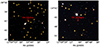 |
Fig. 1. Finder charts composited from LCO observations in gri bands. Left panel: finder chart of SN 2018xx. Right panel: finder chart of SN 2019gbx. The orange circles in both panels represent the calibration standard stars (see Tables A.1 and A.2). |
We applied the lcogtsnpipe (Valenti et al. 2016) and a PyRAF-based pipeline to reduce the observed images of SN 2018xx and SN 2019gbx. Because SN 2018xx and SN 2019gbx are far enough from the center of their host galaxies, we omitted the step of template subtraction. The UBV-band photometry is reported in Vega magnitudes and was converted into the Johnson system using a series of Landolt standard stars observed on the same night (Stetson 2000). The gri-band photometry is reported in AB magnitudes, and we calculated the zero points for the Sloan filters based on the Panoramic Survey Telescope and Rapid Response System (PanSTARRS) catalog (Chambers et al. 2016; Waters et al. 2020) magnitudes of stars in the SN field. For SN 2018xx and SN 2019gbx, the local standard stars with PanSTARRS gri magnitudes and the transformed UBV magnitudes are shown in Tables A.1 and A.2.
Ultraviolet (UV) and optical photometry of these two SNe Ia were also observed with the Neil Gehrels Swift Observatory (Swift; Gehrels et al. 2004) in six bands, including the UVW1, UVW2, UVM2, U, B, and V filters (Roming et al. 2005). According to the zero points of Breeveld et al. (2011) in the Vega magnitudes, we obtained the Swift optical and UV light curves using the data reduction pipeline of the Swift Optical/Ultraviolet Supernova Archive (SOUSA; Brown et al. 2014). We measured the source counts corrected by an average point-spread function using a 3″ aperture. Figure 2 shows the final LCO and Swift light curves of SN 2018xx and SN 2019gbx, and Tables B.1 and B.2 list the flux-calibrated magnitudes.
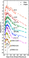 |
Fig. 2. Optical and UV light curves of SN 2018xx (triangles) and 2019gbx (stars). The vertical dashed line indicates the time of the B-band maximum of the two SNe Ia. The phase was measured relative to the maximum brightness. The light curves have been shifted vertically for clarity. |
2.3. Spectroscopy
A total of twelve low-resolution optical spectra of SN 2018xx and eight low-resolution optical spectra of SN 2019gbx were obtained with the FLOYDS spectrographs mounted on the LCO’s two-meter Faulkes Telescope North and South (Sand et al. 2011; Brown et al. 2013). The LCO’s telescope is from the Global Supernova Project (Howell & Global Supernova Project 2017). In addition, two spectra of SN 2019gbx taken by the Yunnan Faint Object Spectrograph and Camera mounted on the Lijiang 2.4-meter telescope (LJT) of Yunnan Astronomical Observatories (Chen et al. 2001; Wang et al. 2019b), including one classification of early spectra, are also included in our analysis. The standard stars observed with airmasses comparable to SN on the same night were applied to calibrate the spectral flux of the above two SNe Ia. The extinction curves at the LCO were used to correct for atmospheric extinction of the spectra, and the telluric absorption lines were also removed from the spectra.
In Sects. 3 and 4, we analyze and compare the light curves and spectra of SN 2018xx and SN 2019gbx. Although these two SNe Ia are quite similar, we identify several key differences. The basic properties of SNe 2018xx and 2019gbx are given in Table 1.
Measured parameters of SN 2018xx and SN 2019gbx.
3. Light curves
3.1. Ultraviolet and optical light curves
The UV and optical light curves of SN 2018xx and SN 2019gbx are shown in Fig. 2. Overall, these two SNe Ia are similar to normal ones in that their light curves both show a pronounced shoulder and secondary maximum in the r and i bands. Like other fast-declining SNe Ia, the light curves of both SN 2018xx and SN 2019gbx reached their peak slightly earlier in the i band and in the UV bands, relative to the B- and g-bands. When applying polynomial fits to the B-band light curves near maximum brightness, we found SN 2018xx reached the B-band peak magnitude of Bmax = 14.48 ± 0.02 mag on MJD 58184.29 ± 0.36, and SN 2019gbx reached the corresponding value of Bmax = 14.63 ± 0.03 mag on MJD 58647.39 ± 0.39. Likewise, these two SNe Ia reached the V-band peak magnitudes of 14.39 ± 0.02 mag (on MJD 58185.29 ± 0.36 for SN 2018xx) and 14.65 ± 0.03 mag (on MJD 58648.40 ± 0.39 for SN 2019gbx). The B-band light curve decline rates (△m15(B)) were measured as 1.48 ± 0.07 mag for SN 2018xx and 1.37 ± 0.07 mag for SN 2019gbx, and the corresponding stretch factors SBV (Burns et al. 2011, 2014) are 0.78 ± 0.04 and 0.84 ± 0.03, respectively. These light curve parameters are also listed in Table 1.
To further study the properties of SN 2018xx and SN 2019gbx, we overplotted the light curves of two well-observed, normal SNe Ia in Figs. 3 and 4, namely, SN 2004eo (△m15(B) = 1.46 mag; Pastorello et al. 2007) and SN 2011fe (△m15(B) = 1.18 mag; Zhang et al. 2016). As can be seen in these figures, SN 2018xx and SN 2019gbx clearly exhibit quite similar light curves. Unlike SN 2011fe, these two SNe Ia seem to have a slightly faster rising pace to the maximums in the U-band and B-band (top panel of Fig. 3) as well as UV (Fig. 4) light curves in their early phases. One can see from Fig. 3 that the light curves of both SN 2018xx and SN 2019gbx show close resemblances to those of the well-observed, fast-declining SN 2004eo in UBVg bands. Nevertheless, these two SNe Ia show noticeable differences in ri bands, especially at the phases around the shoulder or secondary maximum (Fig. 3).
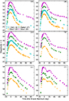 |
Fig. 3. UBVgri-band light curves of SN 2018xx and SN 2019gbx compared with those of the normal SN 2004eo and SN 2011fe. The rest frame light curves of SN 2019gbx and the two SNe Ia have been shifted vertically for greater clarity. |
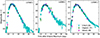 |
Fig. 4. UV light curves of SN 2018xx and SN 2019gbx compared with the well-observed normal SN 2011fe. The rest frame light curves of SN 2019gbx and SN 2011fe have been shifted vertically to match the peak magnitudes of SN 2018xx. |
3.2. Reddening and color curves
Assuming the extinction law RV = 3.1 (Cardelli et al. 1989) and the Galactic reddening of E(B − V)gal = 0.09 mag for SN 2018xx and E(B − V)gal = 0.05 mag for SN 2019gbx, the line-of-sight Galactic extinction (AB) of SN 2018xx and SN 2019gbx can be deduced as 0.39 mag and 0.15 mag, respectively (Schlafly & Finkbeiner 2011). The B − V color of SN 2018xx was estimated to be −0.08 ± 0.07 mag at the maximum light, while that of SN 2019gbx was estimated as −0.02 ± 0.04 mag, both of which agree with the typical values of normal SNe Ia (Phillips et al. 1999; Jha et al. 2007; Wang et al. 2009).
Figure 5 shows the fitting results of the multiband light curves of SN 2018xx and SN 2019gbx with the SuperNovae in object oriented Python (SNooPy2; Burns et al. 2011, 2014). The EBV model with st-type was employed to estimate an average host reddening of E(B − V)host = 0.02 ± 0.07 mag for SN 2018xx and E(B − V)host = 0.01 ± 0.07 mag for SN 2019gbx. The negligible host galaxy reddening derived for SN 2018xx and SN 2019gbx is consistent with the nondetectable Na I D absorption features in their spectra, which are consistent with the observed facts that these two SNe are isolated and far away from the center of the host galaxies.
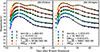 |
Fig. 5. Best-fit light curve model (solid black lines) from SNooPy2 (Burns et al. 2011, 2014) for SN 2018xx (left panel) and SN 2019gbx (right panel). The dashed black lines indicate the 1-σ uncertainty (in many cases smaller than the line width) with respect to the best-fit light curve templates. The light curves have been shifted vertically for greater clarity. |
Figure 6 shows the optical color evolution of SN 2018xx and SN 2019gbx together with that of two well-observed, normal SNe: SN 2011fe and SN 2004eo. The color curves were corrected for reddening due to the Milky Way (Schlafly & Finkbeiner 2011) and the host galaxies. One can see that SN 2018xx and SN 2019gbx are quite similar in color evolution. At early times, both the B − V and g − r color curves reached the bluest color at t ≈ −7 days from the maximum light, and then they evolved progressively redward in a linear fashion until reaching the reddest color at t ≈ +24 days. Both r − i and g − i color curves evolved blueward from t = −9 to +10 days, then they evolved redward again and reach the red peaks at t ≈ +24 days. Later, the color curves gradually evolved blueward as SN 2018xx and SN 2019gbx entered into the early nebular phase.
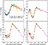 |
Fig. 6. SN 2018xx and SN 2019gbx B − V, r − i, g − r, and g − i color curves compared with those of SN 2004eo (all panels) and SN 2011fe (upper-left panel). All color curves have been corrected for reddening in the Milky Way and the host galaxies using SNooPy2 (Burns et al. 2011, 2014). |
The color curves of SN 2018xx and SN 2019gbx are mostly similar to those of SN 2004eo except that both SN 2018xx and SN 2019gbx are, on average, redder in the early phase and show an extremely different shape in the g − r color curve around the B-band maximum. According to previous studies, redder colors could be indicators of low photospheric temperatures (Nugent et al. 1995; Kasen & Woosley 2007; Zhang et al. 2016). The redder colors at the early phase of these two SNe Ia may suggest that they have lower photospheric temperatures than SN 2004eo (Pastorello et al. 2007). On the other hand, the B − V color curves of SNe 2004eo, 2018xx, and 2019gbx seem to reach their red peaks earlier than those of SN 2011fe.
3.3. Distance and quasi-bolometric light curve
Assuming H0 = 67.8 km s−1, ΩM = 0.308, and ΩV = 0.692, a Tully-Fisher distance obtained for the host galaxy NGC 4767 of SN 2018xx is μ = 33.4 ± 0.40 mag (Theureau et al. 2007), while the distance to the host galaxy MCG-02-33-017 of SN 2019gbx is μ = 33.89 ± 0.06 mag (Smith et al. 2019). We also used SNooPy2 to fit the multiband light curves of SN 2018xx and SN 2019gbx, which gave us an average distance modulus (μ) of μ = 33.07 ± 0.11 mag for SN 2018xx and μ = 33.76 ± 0.10 mag for SN 2019gbx (see Fig. 5). These distance moduli are consistent with the previous results and within the quoted errors. In our study, we adopted the weighted mean distance moduli of μ = 33.09 ± 0.11 mag and μ = 33.86 ± 0.05 mag for SN 2018xx and SN 2019gbx, respectively. With these weighted mean distance moduli, the B-band absolute peak magnitudes of SN 2018xx and SN 2019gbx were derived as Mmax(B) = − 19.00 ± 0.11 mag and Mmax(B) = − 19.38 ± 0.06 mag, respectively, which agree well with those of normal SNe Ia (i.e., Mmax(B)≈ − 19.30 mag; Phillips et al. 1999; Wang et al. 2009). We note that SN 2018xx appears to be fainter than SN 2019gbx around the B-band peak, although they have similar light curves and color curves as well as post-peak decline rates.
Phillips (1993) proposed an empirical width-luminosity relation in which SNe with a wider light curve is usually brighter (Phillips et al. 1999). Kasen & Woosley (2007) found that brighter SNe Ia relative to dimmer ones have broader and more slowly declining light curves in the B-band. According to Kasen & Plewa (2007), SN 2018xx and SN 2019gbx are roughly consistent with this trend. In other words, the relatively faster average value of Δm15(B) for SN 2018xx could be associated with its fainter luminosity.
Based on UV and optical photometry, and hence the spectral energy distribution (SED), including the UVW1, UVW2, UVM2, U, B, V, g, r, and i bands, we established the quasi-bolometric light curves of both SN 2018xx and SN 2019gbx, as shown in Fig. 7. The UV and optical photometry were interpolated with spline interpolation (Ahlberg et al. 1967; Leloudas et al. 2009; Li et al. 2019) in order to complement the missing data whenever necessary. According to the response curves in different filters, the final quasi-bolometric flux was derived by trapezoidal integration over flux densities at different wavebands, which cover the phases from −13.44 to +107.21 days for SN 2018xx and −14.19 to +63.74 days for SN 2019gbx, respectively. One can see from the Fig. 7 that SN 2004eo is more luminous than SN 2018xx and SN 2019gbx in the early phase. According to Kasen & Woosley (2007), there is a positive relation between photospheric temperature (T) and luminosity (L), such as T ∝ L1/4 (and hence  ), again indicating that at the early phase, SN 2018xx and SN 2019gbx have lower photospheric temperatures but a faster increase in temperature. The peak quasi-bolometric luminosities of SN 2018xx and SN 2019gbx were estimated as (1.12 ± 0.08)×1043 and (1.16 ± 0.13)×1043 erg s−1, respectively, and both are similar to that of SN 2011fe (i.e., 1.13 × 1043 erg s−1; Zhang et al. 2016).
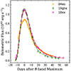 |
Fig. 7. Quasi-bolometric (UV and optical) light curves for SN 2018xx (magenta circles) and SN 2019gbx (green rhombuses) compared with that of SN 2004eo (orange stars) (Pastorello et al. 2007; Li et al. 2022). The solid red curve and dashed dark green curve represent the Arnett (1982) radiation diffusion model of SN 2018xx and SN 2019gbx, respectively. |
The modified radiation diffusion model of Arnett (1982) implemented in the Code Minim (Chatzopoulos et al. 2013) was employed to fit the quasi-bolometric light curves of SN 2018xx and SN 2019gbx via a constant opacity approximation, as shown in Fig. 7. The parameters deduced from the Arnett model include the time of first light (FLT), ejecta mass of radioactive 56Ni (MNi), and light-curve timescale (tlc), which are −13.87 ± 0.02 days, 0.40 ± 0.02 M⊙, and 10.44 ± 0.01 days, respectively, for SN 2018xx (see Chatzopoulos et al. 2012, 2013 for details). The corresponding values derived for SN 2019gbx are FLT = − 14.0 ± 0.03 days, MNi = 0.46 ± 0.03 M⊙, and tlc = 11.3 ± 0.01 days.
We found that the MNi of SN 2018xx is less than that of SN 2019gbx. Moreover, the deduced MNi of the two SNe Ia are smaller than that of SN 2011fe (MNi = 0.57 M⊙; Zhang et al. 2016), but they are close to the lower limit MNi of normal SNe Ia (i.e., 0.4 − 1.1 M⊙; Cappellaro et al. 1997).
4. Optical spectra
Figure 8 shows the spectral evolution of SN 2018xx and SN 2019gbx. From the figure, one can see that the spectra evolution of SN 2018xx and SN 2019gbx are very similar. Based on their similar light curves, color curves, and spectral evolution, we inferred that these two SNe Ia may have experienced physically similar explosions. However, there are still some differences in their spectral features, such as weaker absorption features at shorter wavelengths in the spectra of SN 2018xx and stronger carbon absorption in the early-time spectra of SN 2019gbx. In the following subsections, we discuss the spectral evolution of SN 2018xx and SN 2019gbx further by comparing them with the two well-observed, normal SN 2011fe and SN 2004eo.
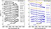 |
Fig. 8. Optical spectral evolution of SN 2018xx and SN 2019gbx. Left panel: spectral series of SN 2018xx collected by LCO telescopes covering the phase from −13.1 to +89.2 days. Right panel: spectral series of SN 2019gbx obtained by LCO (blue) and LJT (orange) spanning the phases from −14 to +37 days. The epochs marked on the right side of the spectra represent the phases in days relative to the B-band maximum light. The vertical dashed lines in both panels indicate the absorption minima of the Si IIλ6355 line in the spectra of SN 2018xx and SN 2019gbx taken at t = +1.37 days and t = +0.92 days, respectively. |
4.1. Temporal evolution of the spectra
Figure 9 presents detailed spectral comparisons performed at four selected epochs (t ≈ −12, −7, 0, and +30 days relative to the B-band maximum). The spectra of SN 2018xx and SN 2019gbx are clearly shown to be mostly different in the blended lines near 4300 Å (Fe II, Mg II) and 4800 Å (Si II, Fe II, Fe III), C II, and O I. At t ≈ −12 days, the blended lines of Fe and Si near 4800 Å of SN 2018xx and SN 2004eo are slightly stronger than those seen in SN 2019gbx and SN 2011fe, as displayed in Fig. 9a. In these early phases, the Si IIλ6355 velocity measured for SN 2018xx is about 15 873 ± 476 km s−1, which is larger than what is found for SN 2019gbx and the comparison SNe Ia. The Ca II near-infrared (NIR) triplet and Ca II H & K absorptions of SN 2018xx and SN 2019gbx are stronger than those of SN 2011fe and SN 2004eo. Also, the absorption features of intermediate-mass elements (IMEs; including Fe, Mg, Si, S, and Ca) dominate the spectra of SN 2018xx and SN 2019gbx. Further inspection of their spectra revealed that SN 2018xx has stronger absorption features near 4300 Å and 4800 Å compared to SN 2019gbx, although the latter has more prominent absorption features of C IIλ6580 and O Iλ7773 relative to SN 2018xx.
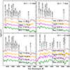 |
Fig. 9. Spectra of SN 2018xx and SN 2019gbx compared with spectra of the other NV SN 2004eo (Pastorello et al. 2007) and SN 2011fe (Zhang et al. 2016) at t ≈ −12, −7, 0, and +30 days (relative to B-band maximum). All the spectra have been corrected for redshift and reddening from their host galaxies and have been shifted vertically for clarity. |
Figure 9b shows the comparison of the spectra one week before the maximum brightness. The absorption strengths of the IMEs increased in all spectra. For the C II absorption feature, it becomes almost invisible in the spectra of SN 2018xx and SN 2019gbx, although it is still detectable in SN 2011fe. The Si IIλ4000 absorption feature is more prominent in SN 2018xx and SN 2019gbx. On the other hand, the Ca II NIR triplet and Ca II H&K absorption features are weaker in all spectra at this phase, and the Ca II NIR triplet absorption of SN 2018xx and SN 2019gbx are weaker than that of SN 2011fe and SN 2004eo. For SN 2004eo, the line velocity of Si IIλ6355 appears lower than those of the comparison SNe Ia. At this phase, the differences between SN 2018xx and SN 2019gbx are mainly near 4300 Å and 7773 Å.
Figure 9c shows the comparison near the B-band maximum. The Ca II NIR absorption features of the comparison SNe Ia gain strength with the receding photosphere. At this phase, the photospheric component of O Iλ7773 begins to emerge in the spectra of SN 2018xx. The blended lines near 4800 Å of Fe II, Fe III, and Si II are still notable in all comparison SNe Ia, while the "W"-shaped S II absorption features and Si IIλ4000 become more prominent at this phase. The photospheric velocities of SN 2018xx and SN 2019gbx measured from the absorption minimum of Si IIλ6355 absorption around the B-band maximum are 10, 482 ± 314 km s−1 and 10, 447 ± 314 km s−1, respectively, which puts both of them in the NV subclass according to the classification scheme proposed by Wang et al. (2009).
We further compared the line-strength ratio of Si IIλ5972 to Si IIλ6355 (R(Si II); Nugent et al. 1995), which was estimated as 0.26 ± 0.02 for SN 2018xx and 0.22 ± 0.01 for SN 2019gbx. These values are slightly larger than that of NV SN 2011fe (0.15 ± 0.02), which was also calculated using multiple Gaussian functions of Zhao et al. (2015, 2016), suggesting that the two SNe Ia have relatively cooler ejecta and lower photospheric temperature (Nugent et al. 1995). In addition, SN 2018xx and SN 2019gbx are also consistent with the tendency that fast-declining SNe Ia generally have larger values of R(Si II) (Benetti et al. 2005; Zeng et al. 2021a).
Figure 9d presents a comparison of the spectra at t ≈ +30 days after the B-band maximum. One can see that all comparison SNe Ia have well-developed absorption profiles and uniform morphologies. With the receding photosphere, the absorption features of the Ca II NIR triplet still dominate in the spectra, but the Fe II features have become more prominent, and they gradually dominate in the wavelength range from 4700 Å to 5000 Å. At this phase, the differences between SN 2018xx and SN 2019gbx are still noticeable in the blended lines near 4300 Å and 4800 Å, similar to what we had observed at early times. Although the Ca II NIR triplet of different SNe Ia is usually distinct at earlier epochs, they evolve into a quite smooth and similar absorption profile during the early nebular phase.
4.2. Ejecta velocity
The ejecta velocity (v) evolutions measured from Si IIλ6355 for SN 2018xx and SN 2019gbx are displayed in Fig. 10. The velocity evolution of these two SNe Ia are quite similar to each other and lie almost fully within the shaded region defined for normal SNe Ia (Wang et al. 2009). The Si IIλ6355 velocity gradients of these two SNe Ia are measured as 38 and 45 km s−1 d−1 during the period from t ≈ 0 to +10 days, suggesting that they belong to the LVG subgroup (based on the boundary of 70 km s−1 d−1 introduced by Benetti et al. 2005). As presented in Sect. 4.1, the Si II velocities of SN 2018xx and SN 2019gbx measured near the B-band maximum are all within the upper limit of NV SNe Ia (i.e., v < ∼11 800 km s−1; Wang et al. 2009). Thus, we classified SN 2018xx and SN 2019gbx as normal SNe Ia of the LVG and NV subclasses. The basic parameters of these two SNe Ia are listed in Table 1.
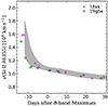 |
Fig. 10. Ejecta velocity evolution of SN 2018xx and SN 2019gbx. The velocities were measured from the minimum of their Si IIλ6355 absorption lines. The shaded region indicates the 1σ uncertainty of the mean velocity curve for NV SNe Ia as derived from Wang et al. (2009). |
5. Discussion
5.1. Properties of the light curves
Rising light curves can be used to put constraints on the radius of the exploding star itself (Piro et al. 2010; Piro & Nakar 2013) by using the estimated FLT (Nugent et al. 2011). In addition, some properties of SN Ia progenitor systems can be examined, such as the scenario of luminosity evolution and interaction with the companion star (Kasen 2010). Using the data at t < −7 days and assuming the same FLT for all six bands (UBVgri), the early multiband light curves of SN 2018xx and SN 2019gbx were fitted by the ideal expanding fireball model, f ∝ (t − FLT)2 (Riess et al. 1999; Conley et al. 2006), as shown in the left and right panels of Fig. 11.
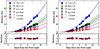 |
Fig. 11. Fit of multiband (UBVgri) early light curves of SN 2018xx (left panel) and SN 2019gbx (right panel). The dashed lines show the expanding fireball model (i.e., f ∝ (t − FLT)2) (Riess et al. 1999) fitting by forcing all six bands to have the same FLT and using the data with t < −7 days. The bottom subpanel in each image displays the residual of the best-fit curves, and the gray dashed horizontal line represents zero residual. |
The FLT relative to the B-band of SN 2018xx fitted from the model is MJD 58168.62 ± 0.07 (−15.7 ± 0.4 days), about 1.8 days earlier than we estimated from using the Arnett model (Arnett 1982), see Sect. 3.3 and Table 1. The dissimilarity could be attributed to the simplifications employed in the Arnett and expanding fireball models. Thus, the average FLT of SN 2018xx was estimated as −14.8 ± 0.2 days. For SN 2019gbx, its FLT fitted by the fireball model is MJD 58631.89 ± 0.10 (−15.5 ± 0.4 days), which is earlier than what was derived using the Arnett model, due to a possible dark phase. The average FLT for SN 2019gbx was estimated as −14.8 ± 0.2 days. Additionally, we found that the rise times of both SN 2018xx and SN 2019gbx were slightly shorter than the average value of normal SNe Ia (Zheng et al. 2017). Zheng et al. (2017) proposed that a shorter rise time generally corresponds to a larger decline rate. The shorter rise times inferred for these two SNe Ia are consistent with their larger decline rates.
In comparison to SN 2019gbx, SN 2018xx seems to have fainter absolute peak magnitudes, which could be attributed to the difference in their progenitor metallicity (Timmes et al. 2003; Foley & Kirshner 2013; Graham et al. 2015). Timmes et al. (2003) found a relation between the initial metallicity of progenitor (Z/Z⊙) and the amount of MNi (i.e., MNi ∝ 1 − 0.057Z/Z⊙). Using this relation, Foley & Kirshner (2013) and Graham et al. (2015) proposed that SNe Ia with higher progenitor metallicity tend to produce a lower MNi and lower absolute peak luminosity. The ∼0.06 M⊙ difference in MNi measured between SN 2018xx and SN 2019gbx perhaps implies a progenitor metallicity difference of Z18xx/Z⊙ = Z19gbx/Z⊙ + 1.05. Alternatively, the lower amount of MNi and fainter absolute peak magnitudes for SN 2018xx may indicate that it has a relatively higher progenitor metallicity. Meanwhile, the lower MNi and larger R(Si II) of SN 2018xx relative to SN 2019gbx may further support its fainter luminosity (Kasen & Woosley 2007).
5.2. Host galaxy
To study the properties of the host galaxies NGC 4767 (for SN 2018xx) and MCG-02-33-017 (for SN 2019gbx), we collected their optical and NIR photometry from the NASA/IPAC Extragalactic Database (NED1) to construct their SEDs. The Flexible Stellar Population Synthesis (FSPS; Conroy et al. 2009; Conroy & Gunn 2010) code in the piXedfit_model module of piXedfit (see Abdurro’uf et al. 2021 for details) was employed to construct the rest frame spectral models with the adopted parameter configurations, including initial mass function (IMF), star formation history (SFH), dust attenuation law, and other optional features (e.g., nebular emission, dust emission, active galactic nucleus dusty torus emission, and intergalactic medium). The adopted SED fitting method of piXedfit is a Bayesian inference technique that provides two kinds of posterior sampling methods: Markov chain Monte Carlo (Acquaviva et al. 2011; Morishita et al. 2019) and random dense sampling of parameter space (RDSPS; Han & Han 2014; Leja et al. 2019).
In this paper, the observed SEDs of NGC 4767 and MCG-02-33-017 were fitted using the piXedfit_fitting module with the Markov chain Monte Carlo method, giving estimates of the stellar mass and evolving age of the stellar population (agesys) of the galaxies. The observed SEDs and the best-fit templates of these two host galaxies are shown in Fig. 12. The stellar mass (M*) of the galaxies NGC 4767 and MCG-02-33-017 were estimated as log and
and  , respectively. And the agesys of these two host galaxies were estimated as log
![Mathematical equation: $ (age_{\mathrm{sys}} / \mathrm{[Gyr]}) \sim 0.90_{-0.21}^{+0.15} $](/articles/aa/full_html/2023/07/aa44985-22/aa44985-22-eq8.gif) and
and  , respectively. Wu & Boada (2019) found that there is a relation between host galaxy stellar mass (M*/M⊙) and metallicity, which can be characterized empirically as
![Mathematical equation: $$ \begin{aligned} {Z = -1.492 + 1.847\log (M_*/M_\odot ) - 0.08026[\log (M_*/M_\odot )]^2}, \end{aligned} $$](/articles/aa/full_html/2023/07/aa44985-22/aa44985-22-eq10.gif) (1)
(1)
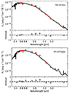 |
Fig. 12. Flexible Stellar Population Synthesis of piXedfit with MCMC fitting for the SEDs of the host galaxies of SN 2018xx (upper panel) and SN 2019gbx (lower panel). The SED plots represent the observed photometric SED (red squares), the median posterior model photometric SED (light gray squares), and the median posterior model spectra (black curve). In the bottom panels are the residuals of the best-fit (dark gray squares). and the zero residual (horizontal black dashed lines). |
where Z is the oxygen abundance 12 +log(O/H). Based on this relation, the supersolar oxygen abundances of NGC 4767 and MCG-02-33-017 were estimated as Z  and
and  , respectively (using a solar value of 8.86; Prieto et al. 2008). We found that the agesys and stellar metallicities estimated for the centers of these two host galaxies are quite similar. Moreover, according to statistical studies of host galaxies, the radial distances (RD in a unit of kiloparsec) have a good correlation with local metallicities, that is, Zlocal = −0.014(±0.016)*RD + Z (Stanishev et al. 2012; Galbany et al. 2016). Applying this correction, the local galaxy metallicities of SN 2018xx and SN 2019gbx could be estimated as
  and
and  , respectively. Therefore, the difference in peak luminosity between SN 2018xx and SN 2019gbx may be caused by the difference in metallicity of their progenitor system, suggesting that the two supernovae may have experienced different combustion intensities during their respective explosions.
5.3. Metallicity interpretation for spectral difference
The spectral evolution is similar for SN 2018xx and SN 2019gbx, although we found differences in their blended lines near 4300 Å, 4800 Å, and C IIλ6580 (Sect. 4.1). Detections of unburned carbon absorption features in the early spectra can help discriminate various explosion mechanisms and progenitor systems of SNe Ia (Yamanaka et al. 2009; Silverman & Filippenko 2012; Li et al. 2019; Zeng et al. 2021b). The fact that the C II features of both SNe Ia are only strong in the earliest spectra indicates that most of the carbon is in the outer layers of the ejecta (Parrent et al. 2012). Heringer et al. (2017) found that the emission from iron can hide the absorption feature of C II, which suggests that the C II absorption feature is more likely to be seen in lower metallicity progenitors or strongly stratified objects of SNe Ia. These explanations support the notion that SN 2018xx with its weaker C II feature relative to SN 2019gbx during the early phase may have a higher metallicity within its outer layers.
The differences in the blended lines near 4300 Å and 4800 Å may be also associated with a difference in elemental abundances of ejecta. We examined the possibility of a metallicity difference further through a spectral fit. The artificial intelligence-assisted inversion (AIAI) algorithm of SNe Ia spectra (Chen et al. 2020) trains a set of neural networks according to the simulated spectra using the Monte Carlo radiative transfer code TARDIS (Kerzendorf & Sim 2014). It has also been used to predict the elemental abundances for SN 2018xx and SN 2019gbx spectra around the B-band maximum. Chen et al. (2020) chose the delayed detonation model (DDT; Khokhlov 1991; Hoeflich et al. 1996) and W7 model (Nomoto et al. 1984) as density profiles of the ejecta to derive an initial guess model (IGM) of the ejecta structure, which was regarded as a baseline model to generate the library of simulated spectra using TARDIS. Additionally, they divided the ejecta structure into four different zones based on distinct velocity boundaries, namely, 5690–10 000 km s−1, 10 000–13 200 km s−1, 13 200–17 000 km s−1, and 17 000–24 000 km s−1. The density profile of the IGM can be approximately visualized as a power-law relation (Chen et al. 2022):
 (2)
(2)
where v is the inner boundary velocity, and texp is the date of explosion. The spectra of SN 2018xx and SN 2019gbx at 1.37 days and 0.92 day show their corresponding texp of 17.07 days and 16.42 days, respectively. For the relation between texp and v derived from Table 1 of Chen et al. (2020), the inner boundary velocities of these two SNe Ia were calculated as ∼7820.6 km s−1 and ∼8118.8 km s−1, respectively. The final input parameter was luminosity, which is sampled from a [8.64, 8.7] uniform distribution in logarithmic space. Based on the predicted elemental abundances, the IGM, the date of explosion, the inner boundary velocity, and target luminosity, we fit the spectra of these two SNe Ia using TARDIS and present the synthesized spectra in Fig. 13. From the figure, one can see that the synthesized spectra are roughly consistent with the observed spectra in the major optical spectral features.
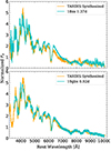 |
Fig. 13. Best-fit TARDIS synthesized spectra (cyan curves) and observed spectra (orange curves) of SN 2018xx (upper panel) and SN 2019gbx (lower panel). Their spectra are at t = 1.37 days and t = 0.92 day, respectively. These spectral fluxes were normalized by dividing their average flux between 6500 Å and 7500 Å for clarity. |
Table 2 lists the Mg, Fe, Si, and C abundances ratios of SN 2018xx and SN 2019gbx inferred from the spectra obtained at around the B-band maximum. The Fe/Mg abundance ratios between SN 2018xx and SN 2019gbx ejections are consistent within the quoted uncertainties, which may indicate that differences in absorption lines observed near 4300 Å may not be solely due to the abundance of Fe II/Mg II in the ejecta. Silverman et al. (2012) mentioned that the Fe II and Mg II features are actually composed of blends of spectral lines from many iron-group elements; thus, the differences near 4300 Å may also be influenced by the other element abundances. In addition, we found that SN 2018xx and SN 2019gbx have a similar Si abundance ratio, which further supports their similarity in Si. The spectra of SN 2018xx and SN 2019gbx at around the B-band maximum have an inconspicuous carbon feature, suggesting that they are likely to be less sensitive to the outermost regions of the ejecta, where carbon may be most abundant. At the B-band maximum light, their spectra have similar blended lines near 4800 Å, which is consistent with similar Fe/Si abundance ratios from Table 2.
Abundance ratios of Mg, Fe, Si, and C for SN 2018xx and SN 2019gbx.
6. Conclusion
In this paper, we presented a study comparing the optical photometric and spectroscopic observations of SN 2018xx and SN 2019gbx. The nearby SN 2018xx has a B-band light curve decline rate of △m15(B) = 1.48 ± 0.07 mag and an absolute B-band peak magnitude of Mmax(B) = − 19.00 ± 0.11 mag, while SN 2019gbx has △m15(B) = 1.37 ± 0.07 mag and Mmax(B) = − 19.38 ± 0.06 mag.
The main conclusions of this study are the following:
-
We classify SN 2018xx and SN 2019gbx as two normal SNe Ia (both NV and LVG subclasses). They share similar light curves, color curves, quasi-bolometric light curves, and spectral evolution.
-
The estimated peak absolute luminosity and the MNi for SN 2018xx are both lower than what is estimated for SN 2019gbx by ∼0.38 ± 0.13 mag and 0.06 ± 0.01M⊙, respectively. This is consistent with Foley & Kirshner (2013), who found that SNe with a higher progenitor metallicity produce a lower MNi and a lower peak luminosity for the same light curve shape. We measured the agesys and stellar metallicity of the host galaxies by piXedfit (Abdurro’uf et al. 2021) for the two SNe Ia, and we found them to be quite similar to each other. Moreover, the metallicities of the local host galaxies of SN 2018xx and SN 2019gbx are estimated to be
 and
and  , respectively, according to an experienced relationship. These findings could indicate that SN 2018xx has a slightly higher progenitor metallicity than SN 2019gbx.
 -
Based on our roughly calculated Mg and Fe abundance ratios of the ejecta from the two SNe Ia, we propose that the difference in the SNe Ia spectra near 4300 Å is related to not only the Fe/Mg abundance in the ejecta but also to the other element abundances. Moreover, SN 2018xx has a weaker carbon absorption rate at early times, which is also in agreement with higher metallicity ejecta.
Future observations and detailed modeling are needed to clarify the physical properties of the intrinsic explosion of these two SNe Ia.
Acknowledgments
Financial support for this work has been provided by the National Natural Science Foundation of China U2031202, 12203029, and the High Level Talent-Heaven Lake Program of Xinjiang Uygur Autonomous Region of China. Xiaofeng Wang is supported by the National Natural Science Foundation of China (NSFC grants 12288102, 12033003, and 11633002), the Scholar Program of Beijing Academy of Science and Technology (DZ:BS202002), and the Tencent Xplorer prize. This work makes use of data from the Las Cumbres Observatory (LCO) network of telescopes. The LCO group is supported by NSF grants AST-1911225, AST-1911151, and NASA grant 80NSSC19K1639. And we thank the staff of the Lijiang 2.4-m telescope (LJT) and Neil Gehrels Swift Observatory (Swift).
References
- Abdurro’uf, Lin, Y. T., Wu, P. F., & Akiyama, M. 2021, ApJS, 254, 15 [CrossRef] [Google Scholar]
- Acquaviva, V., Gawiser, E., & Guaita, L. 2011, ApJ, 737, 47 [NASA ADS] [CrossRef] [Google Scholar]
- Ahlberg, J. H., Nilson, E. N., & Walsh, J. L. 1967, The Theory of Splines and Their Applications (New York: Academic Press) [Google Scholar]
- Arnett, W. D. 1982, ApJ, 253, 785 [Google Scholar]
- Benetti, S., Cappellaro, E., Mazzali, P. A., et al. 2005, ApJ, 623, 1011 [NASA ADS] [CrossRef] [Google Scholar]
- Bloom, J. S., Kasen, D., Shen, K. J., et al. 2012, ApJ, 744, L17 [NASA ADS] [CrossRef] [Google Scholar]
- Branch, D., Fisher, A., & Nugent, P. 1993, AJ, 106, 2383 [NASA ADS] [CrossRef] [Google Scholar]
- Branch, D., Dang, L. C., Hall, N., et al. 2006, PASP, 118, 560 [NASA ADS] [CrossRef] [Google Scholar]
- Breeveld, A. A., Landsman, W., Holland, S. T., et al. 2011, in Gamma Ray Bursts 2010, eds. J. E. McEnery, J. L. Racusin, & N. Gehrels, Am. Inst. Phys. Conf. Ser., 1358, 373 [Google Scholar]
- Brown, T. M., Burleson, B., Crellin, M., et al. 2010, Am. Astron. Soc. Meeting Abstr., 215, 441.06 [NASA ADS] [Google Scholar]
- Brown, T. M., Baliber, N., Bianco, F. B., et al. 2013, PASP, 125, 1031 [Google Scholar]
- Brown, P. J., Breeveld, A. A., Holland, S., Kuin, P., & Pritchard, T. 2014, Ap&SS, 354, 89 [Google Scholar]
- Burns, C. R., Stritzinger, M., Phillips, M. M., et al. 2011, AJ, 141, 19 [Google Scholar]
- Burns, C. R., Stritzinger, M., Phillips, M. M., et al. 2014, ApJ, 789, 32 [Google Scholar]
- Cappellaro, E., Mazzali, P. A., Benetti, S., et al. 1997, A&A, 328, 203 [NASA ADS] [Google Scholar]
- Cardelli, J. A., Clayton, G. C., & Mathis, J. S. 1989, ApJ, 345, 245 [Google Scholar]
- Chambers, K. C., Magnier, E. A., Metcalfe, N., et al. 2016, ArXiv e-prints [arXiv:1612.05560] [Google Scholar]
- Chatzopoulos, E., Wheeler, J. C., & Vinko, J. 2012, ApJ, 746, 121 [Google Scholar]
- Chatzopoulos, E., Wheeler, J. C., Vinko, J., Horvath, Z. L., & Nagy, A. 2013, ApJ, 773, 76 [NASA ADS] [CrossRef] [Google Scholar]
- Chen, D., Wang, J.-C., Xu, J., et al. 2001, Pub. Yunnan Obs., 4, 42 [NASA ADS] [Google Scholar]
- Chen, X., Hu, L., & Wang, L. 2020, ApJS, 250, 12 [NASA ADS] [CrossRef] [Google Scholar]
- Chen, X., Wang, L., Hu, L., & Brown, P. J. 2022, ArXiv e-prints [arXiv:2210.15892] [Google Scholar]
- Conley, A., Howell, D. A., Howes, A., et al. 2006, AJ, 132, 1707 [NASA ADS] [CrossRef] [Google Scholar]
- Conroy, C., & Gunn, J. E. 2010, ApJ, 712, 833 [Google Scholar]
- Conroy, C., Gunn, J. E., & White, M. 2009, ApJ, 699, 486 [Google Scholar]
- Ellis, R. S., Sullivan, M., Nugent, P. E., et al. 2008, ApJ, 674, 51 [NASA ADS] [CrossRef] [Google Scholar]
- Filippenko, A. V. 1997, ARA&A, 35, 309 [NASA ADS] [CrossRef] [Google Scholar]
- Filippenko, A. V., Richmond, M. W., Matheson, T., et al. 1992a, ApJ, 384, L15 [CrossRef] [Google Scholar]
- Filippenko, A. V., Richmond, M. W., Branch, D., et al. 1992b, AJ, 104, 1543 [NASA ADS] [CrossRef] [Google Scholar]
- Foley, R. J., & Kirshner, R. P. 2013, ApJ, 769, L1 [NASA ADS] [CrossRef] [Google Scholar]
- Foley, R. J., Challis, P. J., Chornock, R., et al. 2013, ApJ, 767, 57 [Google Scholar]
- Galbany, L., Stanishev, V., Mourão, A. M., et al. 2016, A&A, 591, A48 [NASA ADS] [CrossRef] [EDP Sciences] [Google Scholar]
- Gehrels, N., Chincarini, G., Giommi, P., et al. 2004, ApJ, 611, 1005 [Google Scholar]
- Graham, M. L., Foley, R. J., Zheng, W., et al. 2015, MNRAS, 446, 2073 [CrossRef] [Google Scholar]
- Han, Y., & Han, Z. 2014, ApJS, 215, 2 [NASA ADS] [CrossRef] [Google Scholar]
- Hatano, K., Branch, D., Lentz, E. J., et al. 2000, ApJ, 543, L49 [NASA ADS] [CrossRef] [Google Scholar]
- Heringer, E., van Kerkwijk, M. H., Sim, S. A., & Kerzendorf, W. E. 2017, ApJ, 846, 15 [NASA ADS] [CrossRef] [Google Scholar]
- Hoeflich, P., Khokhlov, A., Wheeler, J. C., et al. 1996, ApJ, 472, L81 [NASA ADS] [CrossRef] [Google Scholar]
- Howell, D. A. 2011, Nat. Commun., 2, 350 [NASA ADS] [CrossRef] [Google Scholar]
- Howell, D. A., & Global Supernova Project 2017, Am. Astron. Soc. Meeting Abstr., 230, 318.03 [NASA ADS] [Google Scholar]
- Hoyle, F., & Fowler, W. A. 1960, ApJ, 132, 565 [NASA ADS] [CrossRef] [Google Scholar]
- Iben, I. Jr., & Tutukov, A. V. 1984, ApJS, 54, 335 [NASA ADS] [CrossRef] [Google Scholar]
- Jha, S., Kirshner, R. P., Challis, P., et al. 2006, AJ, 131, 527 [Google Scholar]
- Jha, S., Riess, A. G., & Kirshner, R. P. 2007, ApJ, 659, 122 [NASA ADS] [CrossRef] [Google Scholar]
- Jones, D. O., Scolnic, D. M., Foley, R. J., et al. 2019, ApJ, 881, 19 [Google Scholar]
- Kasen, D. 2010, ApJ, 708, 1025 [Google Scholar]
- Kasen, D., & Plewa, T. 2007, ApJ, 662, 459 [NASA ADS] [CrossRef] [Google Scholar]
- Kasen, D., & Woosley, S. E. 2007, ApJ, 656, 661 [NASA ADS] [CrossRef] [Google Scholar]
- Kerzendorf, W. E., & Sim, S. A. 2014, MNRAS, 440, 387 [NASA ADS] [CrossRef] [Google Scholar]
- Khokhlov, A. M. 1991, A&A, 245, 114 [NASA ADS] [Google Scholar]
- Leibundgut, B., Kirshner, R. P., Phillips, M. M., et al. 1993, AJ, 105, 301 [NASA ADS] [CrossRef] [Google Scholar]
- Leja, J., Johnson, B. D., Conroy, C., et al. 2019, ApJ, 877, 140 [NASA ADS] [CrossRef] [Google Scholar]
- Leloudas, G., Stritzinger, M. D., Sollerman, J., et al. 2009, A&A, 505, 265 [NASA ADS] [CrossRef] [EDP Sciences] [Google Scholar]
- Lentz, E. J., Baron, E., Branch, D., Hauschildt, P. H., & Nugent, P. E. 2000, ApJ, 530, 966 [NASA ADS] [CrossRef] [Google Scholar]
- Li, W., Filippenko, A. V., Chornock, R., et al. 2003, PASP, 115, 453 [Google Scholar]
- Li, W., Leaman, J., Chornock, R., et al. 2011, MNRAS, 412, 1441 [NASA ADS] [CrossRef] [Google Scholar]
- Li, W., Wang, X., Vinkó, J., et al. 2019, ApJ, 870, 12 [Google Scholar]
- Li, Z., Zhang, T., Wang, X., et al. 2022, ApJ, 927, 142 [NASA ADS] [CrossRef] [Google Scholar]
- Maoz, D., Mannucci, F., & Nelemans, G. 2014, ARA&A, 52, 107 [Google Scholar]
- Morishita, T., Abramson, L. E., Treu, T., et al. 2019, ApJ, 877, 141 [NASA ADS] [CrossRef] [Google Scholar]
- Nomoto, K., Thielemann, F. K., & Yokoi, K. 1984, ApJ, 286, 644 [Google Scholar]
- Nomoto, K., Iwamoto, K., & Kishimoto, N. 1997, Sci, 276, 1378 [NASA ADS] [CrossRef] [Google Scholar]
- Nugent, P., Phillips, M., Baron, E., Branch, D., & Hauschildt, P. 1995, ApJ, 455, L147 [NASA ADS] [CrossRef] [Google Scholar]
- Nugent, P. E., Sullivan, M., Cenko, S. B., et al. 2011, Nature, 480, 344 [NASA ADS] [CrossRef] [Google Scholar]
- Pakmor, R., Kromer, M., Taubenberger, S., et al. 2012, ApJ, 747, L10 [NASA ADS] [CrossRef] [Google Scholar]
- Parrent, J. T., Howell, D. A., Friesen, B., et al. 2012, ApJ, 752, L26 [NASA ADS] [CrossRef] [Google Scholar]
- Pastorello, A., Mazzali, P. A., Pignata, G., et al. 2007, MNRAS, 377, 1531 [CrossRef] [Google Scholar]
- Paturel, G., Theureau, G., Bottinelli, L., et al. 2003, A&A, 412, 57 [NASA ADS] [CrossRef] [EDP Sciences] [Google Scholar]
- Perlmutter, S., Aldering, G., Goldhaber, G., et al. 1999, ApJ, 517, 565 [Google Scholar]
- Phillips, M. M. 1993, ApJ, 413, L105 [Google Scholar]
- Phillips, M. M., Lira, P., Suntzeff, N. B., et al. 1999, AJ, 118, 1766 [Google Scholar]
- Piro, A. L., & Nakar, E. 2013, ApJ, 769, 67 [NASA ADS] [CrossRef] [Google Scholar]
- Piro, A. L., Chang, P., & Weinberg, N. N. 2010, ApJ, 708, 598 [NASA ADS] [CrossRef] [Google Scholar]
- Podsiadlowski, P., Mazzali, P., Lesaffre, P., Han, Z., & Förster, F. 2008, New A Rev., 52, 381 [NASA ADS] [CrossRef] [Google Scholar]
- Prieto, J. L., Stanek, K. Z., & Beacom, J. F. 2008, ApJ, 673, 999 [NASA ADS] [CrossRef] [Google Scholar]
- Rasio, F. A., & Shapiro, S. L. 1994, ApJ, 432, 242 [NASA ADS] [CrossRef] [Google Scholar]
- Riess, A. G., Press, W. H., & Kirshner, R. P. 1996, ApJ, 473, 88 [Google Scholar]
- Riess, A. G., Filippenko, A. V., Challis, P., et al. 1998, AJ, 116, 1009 [Google Scholar]
- Riess, A. G., Filippenko, A. V., Li, W., et al. 1999, AJ, 118, 2675 [NASA ADS] [CrossRef] [Google Scholar]
- Roming, P. W. A., Kennedy, T. E., Mason, K. O., et al. 2005, Space. Sci. Rev., 120, 95 [NASA ADS] [CrossRef] [Google Scholar]
- Sand, D. J., Brown, T., Haynes, R., & Dubberley, M. 2011, Am. Astron. Soc. Meeting Abstr., 218, 132.03 [NASA ADS] [Google Scholar]
- Sand, D., Strader, J., Chomiuk, L., et al. 2018, TNS Classif. Rep., 2018-259, 1 [Google Scholar]
- Sato, Y., Nakasato, N., Tanikawa, A., et al. 2015, ApJ, 807, 105 [NASA ADS] [CrossRef] [Google Scholar]
- Schlafly, E. F., & Finkbeiner, D. P. 2011, ApJ, 737, 103 [Google Scholar]
- Silverman, J. M., & Filippenko, A. V. 2012, MNRAS, 425, 1917 [NASA ADS] [CrossRef] [Google Scholar]
- Silverman, J. M., Kong, J. J., & Filippenko, A. V. 2012, MNRAS, 425, 1819 [NASA ADS] [CrossRef] [Google Scholar]
- Smith, R. J., Lucey, J. R., Hudson, M. J., Schlegel, D. J., & Davies, R. L. 2000, MNRAS, 313, 469 [NASA ADS] [CrossRef] [Google Scholar]
- Smith, K. W., Srivastav, S., McBrien, O., et al. 2019, TNS AstroNote, 19, 1 [NASA ADS] [Google Scholar]
- Soker, N. 2019, New A Rev., 87 [Google Scholar]
- Stanishev, V., Rodrigues, M., Mourão, A., & Flores, H. 2012, A&A, 545, A58 [NASA ADS] [CrossRef] [EDP Sciences] [Google Scholar]
- Stetson, P. B. 2000, PASP, 112, 925 [Google Scholar]
- Tartaglia, L., Sand, D. J., Valenti, S., et al. 2018, ApJ, 853, 62 [Google Scholar]
- Theureau, G., Hanski, M. O., Coudreau, N., Hallet, N., & Martin, J. M. 2007, A&A, 465, 71 [NASA ADS] [CrossRef] [EDP Sciences] [Google Scholar]
- Timmes, F. X., Brown, E. F., & Truran, J. W. 2003, ApJ, 590, L83 [Google Scholar]
- Tonry, J. L., Denneau, L., Heinze, A. N., et al. 2018, PASP, 130, 064505 [Google Scholar]
- Tonry, J., Denneau, L., Heinze, A., et al. 2019, TNS Discovery Rep., 2019-870, 1 [NASA ADS] [Google Scholar]
- Valenti, S., Howell, D. A., Stritzinger, M. D., et al. 2016, MNRAS, 459, 3939 [NASA ADS] [CrossRef] [Google Scholar]
- Valenti, S., Sand, D. J., & Wyatt, S. 2018, TNS Discovery Rep., 2018-253, 1 [NASA ADS] [Google Scholar]
- Wang, B. 2018, Res. Astron. Astrophys., 18, 049 [Google Scholar]
- Wang, B., & Han, Z. 2012, New A Rev., 56, 122 [CrossRef] [Google Scholar]
- Wang, X., Wang, L., Zhou, X., Lou, Y.-Q., & Li, Z. 2005, ApJ, 620, L87 [NASA ADS] [CrossRef] [Google Scholar]
- Wang, X., Filippenko, A. V., Ganeshalingam, M., et al. 2009, ApJ, 699, L139 [NASA ADS] [CrossRef] [Google Scholar]
- Wang, X., Wang, L., Filippenko, A. V., Zhang, T., & Zhao, X. 2013, Sci, 340, 170 [NASA ADS] [CrossRef] [Google Scholar]
- Wang, X., Chen, J., Wang, L., et al. 2019a, ApJ, 882, 120 [NASA ADS] [CrossRef] [Google Scholar]
- Wang, C.-J., Bai, J.-M., Fan, Y.-F., et al. 2019b, Res. Astron. Astrophys., 19, 149 [CrossRef] [Google Scholar]
- Waters, C. Z., Magnier, E. A., Price, P. A., et al. 2020, ApJS, 251, 4 [NASA ADS] [CrossRef] [Google Scholar]
- Whelan, J., Iben, Icko J., 1973, ApJ, 186, 1007 [CrossRef] [Google Scholar]
- Wu, J. F., & Boada, S. 2019, MNRAS, 484, 4683 [NASA ADS] [CrossRef] [Google Scholar]
- Yamanaka, M., Kawabata, K. S., Kinugasa, K., et al. 2009, ApJ, 707, L118 [NASA ADS] [CrossRef] [Google Scholar]
- Zeng, X., Wang, X., Esamdin, A., et al. 2021a, ApJ, 919, 49 [NASA ADS] [CrossRef] [Google Scholar]
- Zeng, X., Wang, X., Esamdin, A., et al. 2021b, ApJ, 909, 176 [NASA ADS] [CrossRef] [Google Scholar]
- Zhang, J., Lu, K., & Wang, X. 2019, TNS Classif. Rep., 2019-883, 1 [Google Scholar]
- Zhang, K., Wang, X., Zhang, J., et al. 2016, ApJ, 820, 67 [NASA ADS] [CrossRef] [Google Scholar]
- Zhao, X., Wang, X., Maeda, K., et al. 2015, ApJS, 220, 20 [NASA ADS] [CrossRef] [Google Scholar]
- Zhao, X., Maeda, K., Wang, X., et al. 2016, ApJ, 826, 211 [NASA ADS] [CrossRef] [Google Scholar]
- Zheng, W., Kelly, P. L., & Filippenko, A. V. 2017, ApJ, 848, 66 [NASA ADS] [CrossRef] [Google Scholar]
Appendix A: Standards mag
Photometric standards in the SN 2018xx field.
Photometric standards in the SN 2019gbx field.
Appendix B: Observations
Optical and UV photometric observations of SN 2018xx obtained from LCO and Swift telescopes.
Optical and UV photometric observations of SN 2019gbx obtained by LCO and Swift telescopes.
All Tables
Optical and UV photometric observations of SN 2018xx obtained from LCO and Swift telescopes.
Optical and UV photometric observations of SN 2019gbx obtained by LCO and Swift telescopes.
All Figures
|
Fig. 1. Finder charts composited from LCO observations in gri bands. Left panel: finder chart of SN 2018xx. Right panel: finder chart of SN 2019gbx. The orange circles in both panels represent the calibration standard stars (see Tables A.1 and A.2). |
| In the text | |
|
Fig. 2. Optical and UV light curves of SN 2018xx (triangles) and 2019gbx (stars). The vertical dashed line indicates the time of the B-band maximum of the two SNe Ia. The phase was measured relative to the maximum brightness. The light curves have been shifted vertically for clarity. |
| In the text | |
|
Fig. 3. UBVgri-band light curves of SN 2018xx and SN 2019gbx compared with those of the normal SN 2004eo and SN 2011fe. The rest frame light curves of SN 2019gbx and the two SNe Ia have been shifted vertically for greater clarity. |
| In the text | |
|
Fig. 4. UV light curves of SN 2018xx and SN 2019gbx compared with the well-observed normal SN 2011fe. The rest frame light curves of SN 2019gbx and SN 2011fe have been shifted vertically to match the peak magnitudes of SN 2018xx. |
| In the text | |
|
Fig. 5. Best-fit light curve model (solid black lines) from SNooPy2 (Burns et al. 2011, 2014) for SN 2018xx (left panel) and SN 2019gbx (right panel). The dashed black lines indicate the 1-σ uncertainty (in many cases smaller than the line width) with respect to the best-fit light curve templates. The light curves have been shifted vertically for greater clarity. |
| In the text | |
|
Fig. 6. SN 2018xx and SN 2019gbx B − V, r − i, g − r, and g − i color curves compared with those of SN 2004eo (all panels) and SN 2011fe (upper-left panel). All color curves have been corrected for reddening in the Milky Way and the host galaxies using SNooPy2 (Burns et al. 2011, 2014). |
| In the text | |
|
Fig. 7. Quasi-bolometric (UV and optical) light curves for SN 2018xx (magenta circles) and SN 2019gbx (green rhombuses) compared with that of SN 2004eo (orange stars) (Pastorello et al. 2007; Li et al. 2022). The solid red curve and dashed dark green curve represent the Arnett (1982) radiation diffusion model of SN 2018xx and SN 2019gbx, respectively. |
| In the text | |
|
Fig. 8. Optical spectral evolution of SN 2018xx and SN 2019gbx. Left panel: spectral series of SN 2018xx collected by LCO telescopes covering the phase from −13.1 to +89.2 days. Right panel: spectral series of SN 2019gbx obtained by LCO (blue) and LJT (orange) spanning the phases from −14 to +37 days. The epochs marked on the right side of the spectra represent the phases in days relative to the B-band maximum light. The vertical dashed lines in both panels indicate the absorption minima of the Si IIλ6355 line in the spectra of SN 2018xx and SN 2019gbx taken at t = +1.37 days and t = +0.92 days, respectively. |
| In the text | |
|
Fig. 9. Spectra of SN 2018xx and SN 2019gbx compared with spectra of the other NV SN 2004eo (Pastorello et al. 2007) and SN 2011fe (Zhang et al. 2016) at t ≈ −12, −7, 0, and +30 days (relative to B-band maximum). All the spectra have been corrected for redshift and reddening from their host galaxies and have been shifted vertically for clarity. |
| In the text | |
|
Fig. 10. Ejecta velocity evolution of SN 2018xx and SN 2019gbx. The velocities were measured from the minimum of their Si IIλ6355 absorption lines. The shaded region indicates the 1σ uncertainty of the mean velocity curve for NV SNe Ia as derived from Wang et al. (2009). |
| In the text | |
|
Fig. 11. Fit of multiband (UBVgri) early light curves of SN 2018xx (left panel) and SN 2019gbx (right panel). The dashed lines show the expanding fireball model (i.e., f ∝ (t − FLT)2) (Riess et al. 1999) fitting by forcing all six bands to have the same FLT and using the data with t < −7 days. The bottom subpanel in each image displays the residual of the best-fit curves, and the gray dashed horizontal line represents zero residual. |
| In the text | |
|
Fig. 12. Flexible Stellar Population Synthesis of piXedfit with MCMC fitting for the SEDs of the host galaxies of SN 2018xx (upper panel) and SN 2019gbx (lower panel). The SED plots represent the observed photometric SED (red squares), the median posterior model photometric SED (light gray squares), and the median posterior model spectra (black curve). In the bottom panels are the residuals of the best-fit (dark gray squares). and the zero residual (horizontal black dashed lines). |
| In the text | |
|
Fig. 13. Best-fit TARDIS synthesized spectra (cyan curves) and observed spectra (orange curves) of SN 2018xx (upper panel) and SN 2019gbx (lower panel). Their spectra are at t = 1.37 days and t = 0.92 day, respectively. These spectral fluxes were normalized by dividing their average flux between 6500 Å and 7500 Å for clarity. |
| In the text | |
Current usage metrics show cumulative count of Article Views (full-text article views including HTML views, PDF and ePub downloads, according to the available data) and Abstracts Views on Vision4Press platform.
Data correspond to usage on the plateform after 2015. The current usage metrics is available 48-96 hours after online publication and is updated daily on week days.
Initial download of the metrics may take a while.