| Issue |
A&A
Volume 693, January 2025
|
|
|---|---|---|
| Article Number | A54 | |
| Number of page(s) | 23 | |
| Section | Planets, planetary systems, and small bodies | |
| DOI | https://doi.org/10.1051/0004-6361/202452310 | |
| Published online | 03 January 2025 | |
The COBREX archival survey: Improved constraints on the occurrence rate of wide-orbit substellar companions
I. A uniform re-analysis of 400 stars from the GPIES survey
1
LESIA, Observatoire de Paris, Université PSL, CNRS, Sorbonne Université,
Université Paris Cité, 5 place Jules Janssen,
92195
Meudon,
France
2
Univ. Grenoble Alpes, CNRS-INSU, Institut de Planétologie et d’Astrophysique de Grenoble (IPAG) UMR 5274,
Grenoble
38041,
France
3
Centre de Recherche Astrophysique de Lyon (CRAL) UMR 5574, CNRS, Univ. de Lyon,
Univ. Claude Bernard Lyon 1, ENS de Lyon,
69230
Saint-Genis-Laval,
France
★ Corresponding author; This email address is being protected from spambots. You need JavaScript enabled to view it.
Received:
19
September
2024
Accepted:
7
November
2024
Abstract
Context. Direct imaging (DI) campaigns are uniquely suited to probing the outer regions around young stars in pursuit of giant exoplanet and brown dwarf companions, providing key complementary information to radial velocity (RV) and transit searches for demographic studies. However, the critical 5–20 au region, where most giant planets are thought to form, remains poorly explored, as it lies between current RV and DI capabilities.
Aims. Significant gains in detection performances can be attained at no instrumental cost by means of advanced post-processing techniques. In the context of the COBREX project, we have assembled the largest collection of archival DI observations to date with the aim of undertaking a large and uniform reanalysis. In particular, this paper details the reanalysis of 400 stars from the Gemini Planet Imager Exoplanet Survey (GPIES) operated at GPI@Gemini South.
Methods. Following the prereduction of raw frames, the GPI data cubes were processed by means of the PACO algorithm. Candidates were identified and vetted based on multi-epoch proper motion analysis (whenever possible) and by means of a suitable color-magnitude diagram. The conversion of detection limits into detectability maps allowed us to estimate the unbiased occurrence frequencies of giant planets and brown dwarfs.
Results. We derived deeper detection limits than those reported in the literature, with up to a two-fold gain in minimum detectable mass, compared to previous GPI-based publications. Although no new substellar companion was confirmed, we identified two interesting planet candidates awaiting follow-up observations. We derived an occurrence rate of 1.7−0.7+0.9% for 5 MJup < m < 13 MJup planets in 10 au < a < 100 au. This rises to 2.2−0.8+1.0% when including substellar objects up to 80 MJup. Our results are in line with the literature, but with lower uncertainties, thanks to the enhanced detection sensitivity. We confirm, as hinted at by previous studies, a more frequent occurrence of giant planets around BA hosts compared to FGK stars. Moreover, we tentatively observe a smaller occurrence of brown dwarf companions around BA stars, although larger samples are needed to shed light on this point.
Conclusions. While awaiting the wealth of data anticipated from future instrument and facilities, valuable information can still be extracted from existing data. In this regard, a complete reanalysis of SPHERE and GPI data is expected to provide the most precise demographic constraints ever provided by direct imaging.
Key words: techniques: high angular resolution / planets and satellites: detection / planets and satellites: gaseous planets / brown dwarfs
© The Authors 2025
 Open Access article, published by EDP Sciences, under the terms of the Creative Commons Attribution License (https://creativecommons.org/licenses/by/4.0), which permits unrestricted use, distribution, and reproduction in any medium, provided the original work is properly cited.
This article is published in open access under the Subscribe to Open model. This email address is being protected from spambots. You need JavaScript enabled to view it. to support open access publication.
1 Introduction
Bolstered by more than 5000 confirmed detections to date, the exoplanet field has become mature enough to accompany the still thriving detection-oriented endeavor with follow-up studies aimed at shedding light on key questions related to the origin, prevalence, and architecture of planetary systems. By unveiling statistical trends in the measured physical, orbital, and star-related properties of the exoplanet population, exoplanet demographics seeks to connect theory and observation, to gain a fuller understanding of the physical processes underlying planet formation (Biazzo et al. 2022).
The census of known exoplanets currently spans about four magnitudes in mass and in semi-major axis1. No single detection method is adequate to probe such a large extent of the parameter space: the large-scale picture can be unveiled and reconstructed through the combination of the different methods, each optimized for detection inside a specific niche (see, e.g., Gratton et al. 2023, 2024). However, obtaining a complete and unbiased blend from heterogeneous ingredients is hindered by factors such as inconsistent detection criteria, completeness and false-positive assessment, uncertainty quantification, neglect of underlying selection or observational biases (Gaudi et al. 2021).
Whenever two different methods can be simultaneously employed, their complementarity allows for a better characterization of individual objects (see, e.g., Gandolfi et al. 2017; Bonnefoy et al. 2018; Bourrier et al. 2018; Lacedelli et al. 2021; Kuzuhara et al. 2022; Philipot et al. 2023, Lagrange et al. under review) and strengthening the statistical trends emerging in each of the methods (Rogers 2015; Santerne et al. 2016). In cases where different techniques probe different separations within the same system instead, the joint analysis opens up the possibility for exquisite dynamical and formation studies (see, e.g., Covino et al. 2013; Bryan et al. 2016; Zhu & Wu 2018).
Radial velocity (RV) surveys have provided invaluable constraints on the physical and orbital properties of giant planets up to ~5 au (Wolthoff et al. 2022; Rosenthal et al. 2024). Yet, the reliability of RV trends for larger separations has been questioned (Lagrange et al. 2023), while the predicted yields for direct imaging (DI) surveys based on extrapolations of RV results have been shown to be too optimistic (see, e.g., Cumming et al. 2008; Dulz et al. 2020). On the other hand, direct imaging (DI) is mostly sensitive to young giant planets in wide (a ≳ 20 au) orbits, providing access to the scarcely studied outskirts of planetary systems. Starting from 2004 (Chauvin et al. 2004), direct imaging has discovered ~30 planets (M < 13 MJup; Zurlo 2024), including iconic systems such as the disk-enshrouded PDS 70 (Keppler et al. 2018), the ~20-Myr-old β Pictoris (Lagrange et al. 2009), 51 Eridani (Macintosh et al. 2015), AF Leporis (Mesa et al. 2023; De Rosa et al. 2023; Franson et al. 2023), and four-planet HR 8799 (Marois et al. 2008). These detections are the main outcome of large blind surveys targeting tens (e.g., MASSIVE, Lannier et al. 2016; SEEDS, Uyama et al. 2017; LEECH, Stone et al. 2018) or hundreds of stars (e.g., NICI-PCF, Liu et al. 2010; IDPS, Galicher et al. 2016; ISPY-NACO, Launhardt et al. 2020). The forefront of DI surveys, enabled by the exquisite performances of imagers and integral field spectrographs, coupled with extreme AO systems mounted on 8-m class telescopes, is currently represented by the 400 and 600 stars, respectively, from the SpHere INfrared survey for Exoplanets (SHINE; Chauvin et al. 2017) and the Gemini Planet Imager Exoplanet Survey (GPIES; Nielsen et al. 2019) surveys.
By constraining the overall frequency and the properties of wide-separation giant planets, DI studies are expected to enable a thorough comparison with concurrent formation models (see, e.g., Bowler 2016; Vigan et al. 2021). For instance, orbital properties shed light upon their formation and dynamical evolution (Bowler et al. 2020), and the dependence of frequency on stellar mass provides clues about the initial state of the disk and the formation mechanisms at play (Nielsen et al. 2019; Janson et al. 2021). However, despite years of extensive searches, it is still not clear whether the main formation channel for the observed wide-orbit population would be core accretion (CA; Pollack et al. 1996; Mordasini et al. 2009) (the bottom-up process responsible for the formation of planets in the Solar System) or rather a top-down star-like scenario such as gravitational instability (GI; Boss 1997; Vorobyov 2013). While an interplay between the two scenarios is deemed to be favored by empirical parametric models (Reggiani et al. 2016; Vigan et al. 2021) and direct comparisons with synthetic planet populations (Vigan et al. 2021) alike, grasping a clear understanding of how each known companion was formed is still beyond reach. The large uncertainties still existing in the interpretation of the observed picture can be attributed (at least partially) to the fact that the critical 5–20 au region, where most giant planets are thought to form, remains poorly explored. The reason is that this region is situated exactly between the current RV and DI capabilities.
Under given observing conditions, the final performances attainable by a high-contrast imaging observation are dictated both by instrumental (e.g., the telescope, the science instrument, the performance of adaptive optics and coronagraphs) and postprocessing (the algorithms applied to science images to decrease the level of systematic and random noise) components (Galicher & Mazoyer 2024). Depending on observing conditions, stellar brightness and angular separation, state-of-the-art instruments such as the Spectro-Polarimetric High-Contrast Exoplanet Research (SPHERE; Beuzit et al. 2019) and the Gemini Planet Imager (GPI; Macintosh et al. 2014b) typically achieve raw planet-to-star contrasts as low as 10−3−10−5 (Poyneer et al. 2016; Courtney-Barrer et al. 2023). On the instrumental side, 30-m-class telescopes and space-borne coronagraphic instruments are expected to bring about a major leap forward for the field in the next decade (see, e.g., Kasdin et al. 2020; Kasper et al. 2021); upgrades of existing instruments such as SPHERE+ (Boccaletti et al. 2022) and GPI 2.0 (Chilcote et al. 2018) are going to represent the forefront in the medium term. On the reduction side, advanced post-processing algorithms have been already shown to increase the contrast by as much as two orders of magnitudes compared to prereduced data. Therefore, the developments of more powerful reduction techniques can greatly increase detection capabilities working on observations that already exist (see, e.g., Currie et al. 2023).
In the framework of the COupling data and techniques for BReakthroughs in EXoplanetary systems exploration (COBREX) project, we collected more than a thousand archival SPHERE and GPI observations, assembling the largest exoplan-etary direct imaging survey to date, with the aim of rereducing them in a uniform and self-consistent way. The results of the full rereduction of the SHINE survey are illustrated in Chomez et al. (2024). In this work, we present the rereduction of 400 stars coming from GPIES. Despite being the largest DI observational campaign to date, just two new substellar objects were discovered during the survey: one planet (51 Eri b; Macintosh et al. 2015) and one brown dwarf (HR 2562 B; Konopacky et al. 2016). A statistical analysis of the first 300 stars was performed Nielsen et al. (2019; hereafter, N19). By combining the two surveys, it will be possible to obtain the tightest constraints to date on the occurrence of wide-orbit giant planets, thus providing an ideal test-bed for scrutinizing planet formation models.
This paper is organized as follows. We lay out the selection criteria for the sample and the corresponding observations (Section 2.2). We explain how we uniformly derived the stellar parameters of interest (Section 2.3), and we describe the process of data reduction in detail (Section 2.4). Section 3 presents the results of the analysis, namely, companion candidates and completeness maps. The derived occurrence rates are presented and discussed in Section 3.4. A thorough comparison with the literature is the subject of Section 4. Finally, in Section 5, we summarize the results of this work.
2 Data
2.1 Raw data collection
The observations considered in this work were collected between 2013 and 2020 by means of GPI at the Gemini South telescope. GPI is an integral-field spectrograph (IFS) with low spectral resolution (~50; Maire et al. 2014), operating in the wavelength range [0.97−2.40] µm. As the vast majority of GPI observations were gathered in the H band ([1.5−1.8] µm) – with the other bands being mostly used for characterization purposes – (Ruffio et al. 2017) we decided to restrict our query to H-band observations.
We downloaded therefore all H-band raw frames from GPI that are publicly available on the Gemini archive2(~30 000 frames)3. We neglected observational sequences with (at most) 5 frames (typically corresponding to ≲5-min exposure times) and observations of stars only taken for calibration purposes (easily identifiable through their program ID). The reason behind this choice is twofold: on the one hand, the known multiplicity of these stars is expected to detrimentally affect the performances attainable by post-processing; on the other hand, the selection criteria for these stars are different from those of science targets, thereby inducing a bias when interested in statistical considerations.
The preliminary sample obtained in this way (hereafter, GPI database) is composed of 852 sequences for 655 stars. Most of the observations (715/852) within the database were collected in the course of GPIES, and additional 10 sequences are describable as follow-up observations of interesting stars from the campaign. Intertwined to GPIES observations, the remaining 127 sequences were gathered over the lifetime of the instrument as part of other scientific programs. In the following Section 2.2, we elucidate how the final stellar sample was assembled and the criteria a sequence had to meet to be included in the corresponding sample of observations.
2.2 Sample definition
As with any other direct imaging search to date, GPIES was constructed by looking for young stars in the solar neighborhood; the reason for this is that recently formed exoplanets and brown dwarfs are brighter and hotter than mature objects of the same mass due to residual formation heat, yielding a significantly more favorable planet-to-star contrast in near infrared bands. In particular, the stellar sample was assembled by merging lists of members of young moving groups from the literature (de Zeeuw et al. 1999; Zuckerman et al. 2001, 2011) with close (<100 pc) stars selected for large X-ray emission. Echelle spectra were obtained for ~2000 stars to further identify additional young stars based on lithium abundance and chromospheric activity (see Section 2.3 for details). After removing apparent binaries with an angular separation ∊ [0.02″, 3″] and ∆mag < 5 (both before and during the campaign), and accounting for some new association members, a sample of 602 stars was finally obtained (Nielsen et al. 2019).
Due to the decommissioning of GPI – currently undertaking major upgrades to become GPI 2.0 (Chilcote et al. 2020) – in early 2020, the GPIES survey was never completed (~10% of the stars lack observations). It is thus vital to ascertain whether the sample of observed stars be an unbiased extraction of the full sample. An automated target-picker was employed to suggest the best targets for every telescope night, as a function of both observing conditions and stellar age/distance (McBride et al. 2011); however, we verified through a Kolmogorov-Smirnov test (α = 0.05) that the age and distance distributions of the first 300 stars (those from N19) are compatible with those of the full sample of observed stars (page ≈ 1, pdist = 0.051). Additionally, stars with known companions were not prioritized in their first-epoch observation (Nielsen et al. 2019). We can thus confidently maintain that the available GPIES observations are not affected by selection biases, making the sample suitable for statistical studies.
The definition of the final sample was based on a combination of observational constraints and physical constraints on stellar properties. As regards the former aspect, a minimum amount of parallactic angle rotation ∆PA ~ 10° is required to enable efficiently using angular differential imaging (ADI) during post-processing (Marois et al. 2006): we conservatively adopt a minimum rotation of 12° in order to exploit angular differential imaging (ADI) during post-processing4. A single observation with extremely bad seeing was removed. With respect to the latter, we only retained stars for which youth can be established with reasonable confidence (see Section 2.3).
Given our ignorance about the selection criteria adopted for stars from non-GPIES programs, we decided not to consider them for the purpose of this paper. However, we retained non-GPIES observations of GPIES stars as valuable follow-up epochs for promising point-source candidates. The final sample employed throughout this work consists of 400 stars (515 sequences).
2.3 Stellar parameters
The knowledge of stellar ages is pivotal to a meaningful interpretation of direct imaging campaigns, as a large degeneracy exists between age and mass – let alone additional parameters such as metallicity or a planet’s formation history – for substellar objects for which only photometric data are available (see, e.g., Spiegel & Burrows 2012).
Our primary age diagnostics is provided by kinematic membership to young associations and moving groups (hereafter, YMGs). Starting from Gaia DR3 (hereafter, Gaia; Gaia Collaboration 2023) data, we used BANYAN Σ (Gagné et al. 2018b) to classify a star as a member of a YMG when the associated membership probability was p > 90%. A second indicator was represented by the ages obtained by N19: we stress that the underlying data are not public and the derived ages (without error bars) are only available for the 300 stars presented in that study. Finally, the ages for 21 additional stars – that are not members of YMG nor targets of N19 – could be recovered after cross-matching our sample with SHINE (Desidera et al. 2024), which provides a thorough analysis based on a manifold variety of indicators such as isochrones, YMG membership, activity, and lithium abundance. For ages based on N19, that come with no associated uncertainty, we adopt a constant fractional uncertainty of 25%, empirically tuned to match the typical fractional uncertainty for SHINE stars.
Individual stellar parameters for each star were obtained by means of MADYS5 (v1.2, Squicciarini & Bonavita 2022), a tool for (sub)stellar parameter determination based on the comparison between photometric measurements and isochrone grids derived from theoretical (sub)stellar models. Assuming the ages described above, photometry from Gaia DR3 and 2MASS (Skrutskie et al. 2006) – corrected by extinction by integrating the 3D map by Leike et al. (2020) along the line of sight – was compared to the last version of non-rotating, solar-metallicity PARSEC isochrones (Nguyen et al. 2022).
The distance, age and spectral type of the 400 stars are shown in Figure 1. The full collection of the derived properties is summarized in Table A.1, while the ages adopted for YMGs are provided in Table A.2.
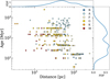 |
Fig. 1 Age of the final stellar sample as a function of distance. The color scale labels different spectral types. Kernel density estimates for the distribution of the two properties are provided on top and to the right of the main plot. |
2.4 Data reduction
2.4.1 Preliminary steps
The prereduction of raw GPI data is performed in two steps: the goal of the first step is to build a 3D data cube (x, y, λ) starting from the 2D image acquired in the detector plane; the collection of the derived data cubes is then stacked into a final 4D data cube (x, y, λ, t).
As routinely done for GPI data, we employed the version 1.6.0 of the GPI Data Reduction Pipeline (hereafter, DRP; Perrin et al. 2014, 2016; Wang et al. 2018) to handle the first part of the prereduction. After subtracting a dark frame, bad pixels in the image are substituted by interpolated values. The mapping of the ~37 000 small spectra created on the detector by GPI’s lenslet array to the corresponding spaxels of the 3D data cube is determined by means of master wavelength calibrations based on Xenon or Argon lamps, conveniently corrected for mechanical offsets induced by flexure (Wolff et al. 2014). The signal of each spectrum can be thus extracted and stored into the corresponding spaxel (Draper et al. 2014). Subsequent steps correct for small distortion effects of the field of view and for halos induced by residual atmospheric turbulence.
Thanks to a square grid embedded within the pattern of the apodizer, a diffraction pattern of “satellite spots” (hereafter, satspots) – attenuated images of the star – is created in the image. The four first-order satspots, symmetrically situated at ~20λ/D from the star, serve three different purposes: (1) to recenter the frames, by locating the position of the occulted star; (2) to calibrate the flux level of each pixel in the science image; (3) to build a model of the off-axis point spread function (PSF)6 (Wang et al. 2014). The final operations of the DRP deal with the astrometric and photometric characterization of the satellite spots, fitted by a Gaussian PSF template.
The second step of the prereduction deals with stacking up and recentering frames to build the final 4D data cube. In addition to the data cube, three files are thus created: (1) a 4D PSF; (2) a wavelength vector; and (3) a parallactic angle vector, that indicates the rotation of the field of view during the sequence. Indeed, GPI observations are operated in a pupil-stabilized mode (i.e., with no derotator), so as to allow the use of ADI-based post-processing algorithms (see, e.g., Ruffio et al. 2017).
This stage is achieved using PYKLIP (Wang et al. 2015). Compared to the 2.6 version, in our approach, we introduced slight modifications to create output files formatted in a SPHERE-like way as regards the data format, the PSF, and data cube flux, and the FOV orientation (east to the left). In this way, we ensured the harmonization of the future SPHERE+GPI sample while smoothing the I/O integration with the post-processing algorithm (Section 2.4.2). In addition to computing the image center through satspot pattern, PYKLIP estimates satspot flux in a more precise way than the DRP; this is a crucial step for photometric characterization purposes that empirically recomputes the wavelength vector based on the satspot-to-center separation (which scales with λ). We visually checked the goodness of the result for all our images; whenever a specific satspot was not properly fitted (due to intrinsic dimness or systematic problems), thereby inducing centering offsets in one or more frames, we used a specific option of PYKLIP to ignore it during recentering.
As already mentioned, satellite spots are faint images of the target star; the flux ratio between a satspot and the star, or grid ratio, was determined by Wang et al. (2014) to be ∆m = 9.4 ± 0.1 mag through on-sky observations. The ~ 10% uncertainty on the grid ratio turns out to be one of the main factors in the total error budget of GPI spectrophotometry.
We performed several tests to quantify the reliability of the wavelength solution, the image centering and the photometric calibration of the PSF. The accuracy of the DRP wavelength solution was estimated by Wolff et al. (2014) to be 0.032% in H-band, well below the 1 % accuracy needed to achieve a spectral characterization uncertainty <5%. With regard to the wavelength precision, for every sequence, we collected the satspot positions estimated by the DRP, along with the computed separations from PYKLIP’s frame centers, ξ(λ, t, s), then averaged over the temporal axis, t, and the satspot axis s to obtain  . We computed the ratio η = ξ(λ)/λ for every sequence, a value that ought to remain constant. The 50th, 16th, and 84th percentiles of the distribution across the sequences yields
  px/µm, corresponding to a precision of 0.15%.
As regards centering precision, propagation of random uncertainties in PYKLIP yields a centering precision along one axis σc,x = 0.04 px (that is, ~0.06 px in 2D), comparable to the one reported in Wang et al. (2014). However, we identified a systematic deviation of the satspot pattern shape from a square (which is an underlying assumption of PYKLIP’s centering algorithm): the difference between the centers computed from doublets of opposite satspots (xc,13, yc,13) and (xc,24, yc,24), stable over time, is  px. We consider the true center to be distributed according to a uniform distribution between (xc,13, yc,13) and (xc,24, yc,24). The final centering error σc is therefore:
 (1)
(1)
This value was consistently employed when propagating astro-metric uncertainties of detected sources.
Finally, we adopted a platescale of 14.161 ± 0.021 mas px−1 (De Rosa et al. 2020a), assuming it to be stable over time (Tran et al. 2016). With respect to the north offset angle, we used a time-varying value following the prescriptions indicated in Table 4 from De Rosa et al. (2020a).
2.4.2 Post processing – PACO
Prereduced datasets were processed in the COBREX Data Center, an improved version of the High-Contrast Data Center (HC-DC7, formerly SPHERE Data Center, Delorme et al. 2017). Prompted by the promising preliminary results presented in Chomez et al. (2023), we decided to process our archive by means of the PAtch-COvariance algorithm (PACO; Flasseur et al. 2018) in its robust angular and spectral differential imaging (ASDI) mode (Flasseur et al. 2020a,b).
PACO is a post-processing algorithm that employs ASDI to model the spatial and temporal fluctuations of the image background inside small patches through a combination of weighted multivariate (i.e., accounting for the spatio-spectral correlations of the speckles field) Gaussian components. Extensive testing proved that the resulting signal-to-noise (S/N) map is distributed as a normalized Gaussian 𝒩(0, 1), hence naturally providing a statistically grounded detection map upon which > 5σ detections can be identified at a controlled false alarm rate (e.g., at 5σ significance level). The algorithm was shown to be photometrically accurate and robust to false positives, and to outperform reduction methods that are routinely employed for SPHERE (Chomez et al. 2023). For these reasons, PACO was appointed by the SHINE consortium as the main reduction algorithm for the final analysis of the whole survey (Chomez et al. 2024).
In addition to this, the ASDI mode of PACO uses vectors of spectral weights (hereafter, the spectral priors) to maximize the detection capability of candidate sources exhibiting physically representative substellar spectra. As detailed in Chomez et al. (2023), for every star, we generated 20 such priors starting from exoplanet spectra from the ExoREM library (Charnay et al. 2019) (Teſſ ∊ [400, 2000] K) and suitable stellar spectra from the BT-Nextgen AGSS2009 library (Allard et al. 2011).
As in Chomez et al. (2023), extensive injection tests were performed on GPI datasets in order to ensure the reliability of 5σ detection limits, an output provided by PACO after the reduction (Flasseur et al. 2020a). After randomly picking a sample of 10 sequences, 12 synthetic sources were evenly injected in each observation’s FOV; the mean flux of each source was set equal to the 5σ detection limits estimated by PACO at the corresponding coordinates. The whole process was repeated three times, varying the input spectrum – a flat contrast spectrum, a T-type spectrum, and an L-type spectrum8 – of injected sources, yielding a total 360 injected sources. The median S/N of the recovered sources is 5.1, with little variation with respect of spectral type, confirming the statistical reliability of the contrast and detection confidence estimated by PACO and underlying the statistical analysis.
Figure 2 shows the final performances attained by the PACO reduction as 5σ detection limits. We have made these limits publicly available to the community. It is possible to notice that the usage of physically motivated spectral priors does indeed enhance detection capabilities. However, in order to easily allow for comparisons with reductions performed using different algorithms, we conservatively adopt in the following analysis a flat spectral prior, which is a combination of spectral channels assuming that any source has the same spectral energy distribution as its star; this is equivalent to standard SDI-based algorithms.
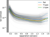 |
Fig. 2 5σ detection limits obtained with PACO. Individual curves are plotted in gray. The median curve is plotted as a light blue solid line, the dashed lines representing the 16 and 84% percentiles of the curve distribution. The orange and green solid lines indicate the median detection limits assuming a T-type and an L-type spectral prior, respectively. The gray box marks the inner working angle of the coronagraphic mask. |
2.4.3 Post processing – cADI
One of the underlying assumptions behind PACO is that the spatial and temporal fluctuations of noise inside patches are much stronger than the additional contribution from physical sources happening to cross the patch itself during the exposure (Flasseur et al. 2018). The assumption breaks down when a bright source, such as a stellar companion, is present. In other words, the algorithm is optimized to detect faint sources but can severely subtract, or even cancel, very bright sources in the derived S/N map. To complete the census of sources at the bright end, we developed a custom routine based on classical angular differential imaging (cADI; Marois et al. 2006) and performed a uniform reduction of the archive. After computing the pixel-wise median frame of the exposure sequence, the routine subtracts it from every frame, then derotates the frames and sums them up both temporally and along wavelength. The 4D PSF is stacked along the temporal axis to build a 3D (x, y, λ) PSF, which is then fitted by a 2D Gaussian model. The reduced map is finally normalized by the peak of the PSF model so as to translate it in contrast units. Detections are automatically performed on the derived map by computing the variance across annuli, centered on the target star, of width equal to 1 px, and finding the pixels of the map beyond a certain threshold level κ (expressed in noise standard-deviation units). In a subsequent step, a more precise characterization by fitting the PSF model provides the astrometry and photometry of each source.
Because of the simplicity of the noise-reduction approach, the S/N distribution in any annulus of a given contrast maps usually shows large deviations from Gaussianity. On the one hand, this issue implies that high thresholds (κ ≳ 20) must be adopted to ensure the stability of the detection step; on the other hand, the poor robustness against outliers intrinsically prevents us from precisely defining a statistically grounded detection threshold.
A visual inspection of all the maps ensured the reliability of the detections. Given the above-mentioned caveats and the neglect of a correction for signal self-subtraction, the derived photometry will only be used to characterize the stellar companions presented in Appendix D.
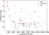 |
Fig. 3 Comparison between PACO and cADI performances. Sources only detected by PACO are shown as blue circles, while sources only seen through cADI are indicated as red diamonds. Common sources are plotted as blue squares with a red edge. |
3 Results
3.1 Exoplanet candidates
The PACO reduction of our sample yielded 91 detected sources. This number does not include a few false positives that could be recognized and removed (see Section 3.2). Then, 11 additional sources were detected through cADI. 62 sources are detected by both methods, ensuring the overlap of the respective dynamical ranges. Figure 3 shows the sources detected by the two methods. Astrometric and photometric details for all the candidates are provided in Table C.1.
Candidate companions in DI observations are always seen as unresolved point-like sources, and no information on their distance can be discerned from a single observation; in other words, it is not clear a priori if a source is physically bound to the target star or is instead a distant background star that happens to be projected close to the target. If two or more epochs are available, the differential motion between the foreground target star (and the objects bound to it) and faraway background stars can be disentangled (Figure 4).
Whenever more than one observation was available in our sample or when additional epochs from SPHERE could be recovered, it was possible to ascertain the proper motion of the candidates: 57 sources from the PACO reduction and 2 sources only detected with cADI were ruled out as background contaminants in this way.
If only a single observation was available or if detection limits allowed for detection in just one epoch, we adopted an alternative vetting criterion that exploits color-magnitude diagrams (CMDs) to identify sources showing similar colors to known imaged planets and to set them apart from background sources. It might be argued that, given the availability of contrast spectra, a spectrum-based classification could be employed: however, we argue that such a method would be highly sensitive to both random uncertainties and the ignorance about the amount of interstellar extinction to be adopted for background-star spectra. Conversely, the photometric method based on CMDs has already been shown to be highly reliable for absolute magnitudes H ≳ 15 mag, using an unprecedented sample of ~2000 of confirmed astrophysical background sources found in SPHERE data (Chomez et al. 2024). This usage of the CMD has been introduced by the SHINE consortium (Chauvin et al. 2017) and its construction is fully detailed in Bonnefoy et al. (2018). This tool has already been used to efficiently classify some of the sources detected in the first part of the SHINE survey (Langlois et al. 2021). As a first step, the H-band spectrum of each target star was estimated by means of synthetic stellar spectra from the BT-Nextgen AGSS2009 library9 (Allard et al. 2011), adequately degraded to match the spectral resolution of GPI. The best-matching synthetic spectrum was identified as the closest in effective temperature; the latter was empirically estimated as the median value across all literature measurements found in VizieR (Ochsenbein et al. 2000). Contrast spectra from candidate sources detected with PACO10 could thus be turned into physical spectra by multiplying them by their corresponding primaries spectra. We convolved these spectra with SPHERE H2 and H3 filters to derive synthetic H2 and H3 photometry for all our candidates; in other words, GPI spectroscopy was turned into SPHERE-like photometry both to exploit the CMD vetting method and to enable future comparisons between the results from the two instruments. The convolution was possible thanks to the broad extent of GPI’s H band, whose wavelength window covers both SPHERE narrow-band H filters.
In this way, it was possible to place every PACO candidate in a (H2-H3, H2) CMD (see Figure 5). We used confirmed background objects from the SHINE survey, which offers a larger sample statistics thanks to the wide 11″ × 11″ field of view of IRDIS (Dohlen et al. 2008), to build an “exclusion zone”. This is defined as the region of the CMD that encompasses all the points within 5σ from the mean colors of background sources as a function of their absolute magnitude. As in SHINE publications, the exclusion zone was set to begin at H2 = 16 mag, as the existence of some planets (e.g., HR 8799 b) with H2 ~ 15 mag and H2 – H3 ~ 0 mag renders the method unreliable at brighter magnitudes (Langlois et al. 2021, Chomez et al. 2024). We labeled the sources lying along the T track or having additional indications hinting towards a bound nature as “companion candidates”, and the sources in the regions of H2 < 16 mag and H2 – H3 ~ 0 as “ambiguous”.
Excluding already known substellar companions, all but nine sources can be confidently ruled out as background contaminants. Seven of these are classified as ambiguous according to our vetting scheme and we do not discuss it further in this paper. The nature of the two remaining promising candidates, whose photometry and age are consistent with 5–8 MJup objects, is currently unclear. The candidate around HIP 78663 is located in a position of the CMD where the colors of bound companions overlay those of background stars; however, we classify it as a promising candidate because of a tentative ~3.5σ detection in the shallower second epoch possibly hinting at common proper motion. As regards the candidate around HD 24072, in addition to the hypothesis of a bound nature, the following scenarios might be envisaged to explain its position along the young-object track:
A free-floating planet or brown dwarf, belonging to the same association as the target and thereby possessing similar colors to substellar companion while not exhibiting a large variation of the distance modulus.
A statistical false positive (see Section 3.2): the spectral dependence of the photocenter of a false positive could be incorrectly detected as a blue source mimicking the spectrum of a real substellar companion lying along the T track.
Spurious detections in direct imaging have previously arisen due to extended objects (proto-planetary and debris disks) that were poorly subtracted (see, e.g., Sallum et al. 2015 and confutation by Currie et al. 2019), but we exclude this possibility given the lack of infrared excess in WISE (Wright et al. 2010) bands.
Finally, we note that the HD 24072 system also comprises a low-mass star, closer to the primary than the planet candidate (see Section D); under the assumption of face-on circular orbits, we empirically verified, based on the results by Musielak et al. (2005), that the candidate would be far enough from the substellar companion to be dynamically stable.
Our reanalysis redetected all substellar companions (seven planets, three brown dwarfs) that we expected to find on the basis of the literature (Figure 6). Some of these companions – notably, HR 8799 c, d, and e – have just one epoch in our observing sample; consistently with the decision tree described above, we would have been able to confirm them as bound objects through proper motion test, employing additional available SPHERE or GPI epochs.
In Table 1, we offer details on the astrometry and the photometry of these ten substellar companions. Given the extensive characterization of these objects already undertaken in the literature, we deem a rederivation of masses and semi-major axes (the main input needed for the statistical analysis of Section 3.4) to be outside of the scope of this paper; instead, we decided to recover the most accurate values from dedicated literature works.
In addition to substellar companions, we detected six sources whose high luminosities point toward a stellar nature. We were able to confirm five of them as physically bound thanks to: (1) a proper motion strongly disagreeing with background stars and (2) astrometric wobbles indicated by the Gaia astrometric solution of the corresponding primaries. The remaining binary candidate to HD 74341B, with no second epoch and too bright to employ the CMD test, is awaiting confirmation. Details are provided in Section D.
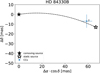 |
Fig. 4 Example of proper motion diagram. The astrometric displacement of the candidate around HD 8433OB between the first and the second epoch is compatible with a background source with null motion (empty star). A bound object would have been in a position close to that marked by the filled star and within the boundaries allowed by a Keplerian motion. |
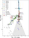 |
Fig. 5 CMD of the companion candidates detected in this work. Over-plotted to known substellar objects (white squares), background stars are represented as yellow stars if identified through proper motion analysis, or as blue circles if recognized via their color. Ambiguous sources are marked as red crosses. The exclusion area (gray) is defined by the two dashed lines. The two promising candidates (from left to right: C1 (HD 24072), C2 (HIP 78663)) are indicated as red dots. |
3.2 False positives
As mentioned in Section 3.1, the roster of PACO candidates does not include a few detections that have been identified as false positives, induced either (1) by real astrophysical or optical features or (2) by statistical fluctuations of the S/N map. The former category includes residuals of the first Airy ring around very bright sources (two cases) and disk residuals (ten cases); the latter (eight cases) is comprised of unusually bright residuals that had no counterpart in additional GPI or SPHERE observations, with better or similar detection limits.
With respect to the latter case, we tried to estimate the number of false positives expected to arise from statistical fluctuations. We recall that the distribution of pixel intensities in PACO S/N maps is a normalized Gaussian 𝒩(0, 1). In this case, a 5σ threshold corresponds to a false alarm probability p5σ = 2.9 ⋅ 10−7. Given the number of pixels in GPI’s FOV, Npx = 1852 and the number of effectively independent spectral priors, Np, which we empirically estimate as Np ≈ 411, using a binomial distribution, we expect ~20 false positives across the entire survey (see Chomez et al. 2023). This number is larger than the number of statistical false positives that could be identified through second-epoch observations; hence, we expect that some sources labeled as CMD background sources also belong to the category.
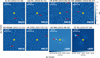 |
Fig. 6 PACO or cADI detection maps for the substellar companions detected in the survey (indicated by arrows). PACO maps are to be read as S/N maps, sharing a common colorbar. Individual colorbars are shown below the two cADI maps. |
3.3 Completeness
The completeness of our survey was quantified in the following way. As a first step, we azimuthally averaged the 2D detection maps provided by PACO, obtaining ID contrast curves (detection limits at 5σ).
Pending a final confirmation of the nature of the two promising candidate companions, the detection limits of the corresponding observations were adjusted accordingly to ensure the statistic reliability of the corresponding observations. The same was done for the seven datasets containing ambiguous sources. In particular, the mean contrast of each candidate was employed as a floor value in the corresponding 2D 5σ map. In other words, we make the assumption of shallower observations, so that a source as bright as the candidate can be (at most) a marginal 5σ detection. These maps were then collapsed to ID, as described above.
The ID curves obtained in this way were converted into mass limits through MADYS, adopting the stellar parameters discussed in Section 2.3. The mass-luminosity relation is based on the ATMO evolutionary models (hereafter, ATMO; Phillips et al. 2020; Chabrier et al. 2023)12. Chemical disequilibrium is expected to critically affect the atmospheric features of cool T-type and Y-type objects (see, e.g. Leggett et al. 2015, 2017; Miles et al. 2020; Baxter et al. 2021). Given that (1) the corresponding temperature range is within the reach of our analysis (see Figure 5) and (2) the effect is particularly strong in H-band observations, such as those under consideration, we decided to employ the grid assuming weak chemical disequilibrium (ATMO-NEQ-W) instead of chemical equilibrium (ATMO-CEQ). We explore in Appendix E the effect of this assumption, comparing the results with those obtained under chemical equilibrium and strong disequilibrium (ATMO-NEQ-S)13. In addition to this, the impact of model selection and age uncertainty was quantified.
Starting from mass limits, the completeness could be estimated through Exo-DMC14 (Bonavita 2020). Within each cell of a 2D grid in the (mass, sma) plane, the detectability of N = 1000 companions to every star, whose orbital parameters are drawn in a Monte Carlo fashion, was computed based on a comparison with the 5σ mass limits as a function of the projected separation. In Table 2, we offer an overview of the adopted parameters.
The final map is computed by taking the average of all the individual maps. When multiple epochs for a given star were available, the largest value for the detectability was selected for every cell. The results are shown in Figure 7. We notice that the peak sensitivity of the survey is about 88%: we interpret such a low value as the combination of three factors: (1) the small field of view of the instrument; (2) the moderate distance spread across the sample; and (3) the fact that when working in terms of semi-major axis (and not in projected separation), a fraction of planets with given a might be undetectable because of projection effects.
We are now able to directly compare our detection capabilities with those of N19, so as to justify a posteriori the idea of a reanalysis of those archival data. In order to avoid any possible systematic difference, a new map was computed only using the observations considered therein. Moreover, instead of using Exo-DMC, we decided to closely reproduce the original method, including the same values for distances, ages, and substellar evolutionary model. The comparison (shown in Figure 8) indicates that the PACO-based reanalysis allows for a significant performance gain at all separations, which can be up to twofold in terms of detectable mass at given completeness.
Detected substellar companions to stars in the sample.
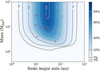 |
Fig. 7 Survey completeness as a function of companion mass and semi-major axis, computed using the ATMO-NEQ-W models. Red stars indicate known substellar companions (see Table 1). |
Input parameters used for Exo-DMC.
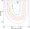 |
Fig. 8 Comparison of the survey completeness between N19 (dashed lines) and this work (solid lines). Only the observations used by N19 were used to draw this plot. |
3.4 Planet occurrence rates
Deriving unbiased occurrence frequencies of exoplanets is one of the main goals of large blind surveys and, in turn, a crucial input to draw comparisons with formation models. Provided a large enough sample, it is additionally possible to investigate the dependence of these frequencies on host properties such as mass and metallicity, highlighting the key role of the parent star in shaping its planetary system.
We begin our investigation by focusing on the occurrence frequency, f, for the entire stellar population represented by the GPIES sample. Extracting this quantity from the fact of having observed N companions given a certain survey completeness is a typical inversion problem that can be treated within a Bayesian framework.
We employed a formalism that is similar to that used in previous direct imaging studies (see, e.g., Lafrenière et al. 2007; Lannier et al. 2016). Given a certain area 𝒜 in the (sma, mass) plane defined by amin < a < amax and mmin < m < mmax, we define pi as the mean probability of observing a companion around the i-th star lying within 𝒜. Based on our completeness analysis (Section 3.3), pi can be estimated as the mean detection probability in 𝒜 across the entire survey; namely, the mean value in 𝒜 of the completeness map shown in Figure 7.
The probability pdet,i to detect a companion in 𝒜 around the i-th star is the product of the detection probability and the underlying occurrence frequency f: pdet,i = pi · f. The connection with the observed planet sample is mediated by d, a vector whose i element represents the number of companions detected within 𝒜 around the i-th star.
The likelihood of the observed data as a function of the f can be estimated as the product of individual Bernoulli events, one per star:
 (2)
(2)
The probability density function of f, that is, the occurrence frequency of companions in 𝒜 given the data, can be finally estimated through Bayes’ theorem:
 (3)
(3)
This gives us the posterior distribution emerging from the interplay between a suitable prior distribution P(f) and the likelihood L({di}|f). We adopted two distinct priors: a uniform prior and a Jeffreys prior. The uniform prior is
![Mathematical equation: $P(f) \propto 1,\quad \forall f \in [0,1]$](/articles/aa/full_html/2025/01/aa52310-24/aa52310-24-eq9.png) (4)
(4)
Despite the fact that it does not incorporate any observational information, this expression is not uninformative, as it assumes much larger weights for large values of f compared to what is expected from observations. Nevertheless, the simplicity of this prior makes it widely adopted in the literature: we decided to employ it in order to allow for comparison with published results.
A Jeffreys prior has the twofold advantage of being non-informative and counterbalancing the bias that favors f ~ 0.5. In the case of Bernoulli events, the Jeffreys prior for the parameter f is simply:
 (5)
(5)
We adopted the latter prior distribution, which offers the advantage of being non-informative, as our standard choice in the following analysis.
A particularly delicate point is represented by the choice of 𝒜: on the one hand, selecting a too narrow range would result in a critical amplification of fluctuations from small number statistics; on the other hand, including regions where <{pi}> ~ 0 would require a significant amount of extrapolation due to the lack of data and, consequently, induce a flattening of the posterior distribution over the prior. An additional factor to take into account is the dependence of the results on both age uncertainty and model selection, becoming more severe as the lower mass limit is decreased (Appendix E). We decided to consider, as our nominal case, a lower mass limit of 5 MJup and a semi-major axis range 10 au < a < 100 au as a compromise between these concurrent factors; the upper mass limit will be set to either 13 MJup or 80 MJup depending on whether brown dwarf companions are considered or not. We derive occurrence frequencies of  when 𝒜 = [5, 13] MJup × [10, 100] au, and
  when 𝒜 = [5, 80] MJup × [10, 100] au, with f represented by the median of the posterior and the error bars defined from the [16%, 84%] percentiles. In order to allow a straightforward comparison with previous results from the literature (Section 4), we also present additional occurrences starting from different definitions of 𝒜 (Table 3). We notice that no significant difference is derived from the prior choice, confirming that our careful choice for 𝒜 did minimize the impact of the prior; the error-bars, as expected, are smaller in Jeffreys case compared to the uniform case. In addition to this, no significant deviation arises for this choice of 𝒜 as an effect of the theoretical assumptions and observational uncertainties, ensuring the robustness of our results (Appendix E).
We assume that the host star metallicity is not a factor of particular concern, as the metallicity of young star-forming regions in the solar neighborhood is typically solar, with limited spread (D’Orazi et al. 2011; Biazzo et al. 2012; Baratella et al. 2020; Magrini et al. 2023). Conversely, as done in Nielsen et al. (2019) and Vigan et al. (2021), we explicitly investigated the dependence of the occurrence frequency on stellar mass. We divided our sample in three bins of stellar masses, obtaining the BA sub-sample (M > 1.5 M⊙, 160 stars), the FGK subsample (0.5 < M < 1.5 M⊙, 235 stars), and the M subsample (M ≤ 0.5 M⊙, 5 stars). Given its small size, the M star sample was discarded.
Both the aggregated results and the mass-dependent ones are plotted in Fig. 9. Occurrence frequencies for different values of 𝒜 are provided for reference in Table 3. Moreover, a digitized version of completeness maps is also made available so as to allow interested readers to extract additional results based on different definitions of 𝒜.
Occurrence rates for different definitions of the (mass, sma) range 𝒜 and for the two choices for the prior distribution (U: uniform; J: Jeffreys). (a)95% upper limit.
4 Discussion
The analysis described in Section 3.4 thus made it possible to directly compare the results emerging from our PACO rereduction of GPI data to previous literature works.
Figure 10 presents a juxtaposition of our results with the frequencies derived from the first 300 stars of GPTES (Nielsen et al. 2019) and the first 150 stars of SHINE (SHINE F150; Vigan et al. 2021). Moreover, the results emerging from the meta-analysis of 384 imaged stars by Bowler (2016) are shown, although we stress that they are by design less protected against selection biases due to the heterogeneous underlying sample. A general finding is that our results are fully compatible with literature estimates, but they are typically more precise. In particular, the comparison with N 19 clearly indicates that the new analysis places the tightest constraints to date on giant planet occurrence based on GPI data, with a gain in precision being a direct consequence of the large gain in completeness (Figure 8). The smaller frequency of companions is an effect of the increased completeness with no new confirmed detection. As regards SHINE F150, the much larger field of view of IRDIS (11″ × 11″, compared to the 2.7″ × 2.7″ FOV of GPI) ensures a much more complete coverage of the semi-major axis range of interest and thus larger room for planet detection, compensating with a twofold advantage for our study in terms of sample size and reduction performances: as a result, the precision of the derived occurrence rates is similar. In this regard, the full analysis of SHINE data with PACO (Chomez et al. 2024), which combines all the advantages of the two analyses, is expected to provide an invaluable contribution to demographic studies of wide-orbit exoplanets.
In view of the profound consequences with respect to planet formation scenarios, it is extremely interesting to assess the dependence of the observed occurrence rates on stellar mass. As in N19, we employed a threshold value of M = 1.5 M⊙ to distinguish a BA subsample and a FGK subsample. That study claimed that a significant (3.4σ) tension between BA and FGK planet rates (fBA and fFGK, respectively) exists for 𝒜 = [2,13] MJup × [3,100] au : = 𝒜1, with planets being more common around BA hosts; while six companions were detected inside 𝒜1 in the BA subsample, no companion was identified in the FGK subsample. However, we expect the result to be weakened by the re-evaluation of the mass of HR 2562 b (Zhang et al. 2023), a companion to an FGK star now firmly placed into the planetary-mass domain. In order to verify whether this is the case, we drew, in a Monte Carlo fashion, values from the posterior distributions of fBA and fFGK under 𝒜1. The values from the latter distribution are larger than those drawn from the former in 0.1% of the cases, implying a 3.3σ tension between the two distributions. Hence, our analysis confirms the finding by N19.
With respect to brown dwarf companions, no statistically significant difference in the observed rates was found by N19 between the BA and FGK hosts. The observation is in line with the results of previous analyses showing compatible rates across a wide range of stella types (see, e.g., Nielsen et al. 2013; Bowler et al. 2015; Lannier et al. 2016; Bowler & Nielsen 2018). Based on our analysis, a tentative (1.7 σ) tension between the two rates is found for 𝒜 = [13,80] MJup × [5,100] au, with an interesting inversion compared to the planetary case: in other words, giant planets appear to be more common around BA host, while brown dwarf companions tentatively appear to be more common around FGK hosts.
Although the BD trend is not statistically significant, an interesting analogy might be drawn with the behavior of the two empirical distributions of substellar companions introduced by Vigan et al. (2021) in the context of SHINE. A planet-like and a star-like distribution of companions – both being the product of a log-normal distribution for semimajor axis and a power-law for companion-to-star mass ratios – were simultaneously fitted to the substellar companion population, divided in three bins of mass (BA, FGK, and M). Similarly to our planetary rates, the median values of the planet-like posterior are larger than those of the star-like posterior for BA hosts, and smaller for FGK hosts. It might be argued that a strict distinction between giant planets and brown dwarfs based on the deuterium burning limit is not adequate to capture the complexity of the different formation mechanisms (CA and GI) involved (Chabrier et al. 2014) and that studying together the entire population is the key to identify population trends (see, e.g., Gratton et al. 2024). While this is certainly true, first-order, population-wise differences in some parameter, arguing for different underlying formation channels, can sometimes be discerned using rough mass boundaries (Bowler et al. 2020).
In view of the low occurrence rates, the large extent of host star masses, the interplay of different formation channels and the impact of input assumptions, we deem it necessary to defer a thorough study of the distribution of companion properties to our future joint SPHERE+GPI analysis. Thanks to its larger sample size, this sample is expected to bring about much tighter constraints on the properties of the companion population, offering in turn the possibility to compare them both to empirical distributions and to synthetic populations of companions produced by formation models.
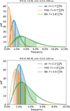 |
Fig. 9 Occurrence frequency of GP (upper panel) and GP+BD (lower panel) from the re-analysis of the 400-star GPIES sample presented in this work. Aggregated results are shown in blue, whereas results for the BA and the FGK subsample are plotted in green and orange, respectively. The colored area encompasses the [16th, 84th] of the posterior distribution. |
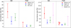 |
Fig. 10 Comparison of the occurrence rates (left panel: 𝒜 = [2,13] MJup × [3,100] au; right panel: 𝒜 = [5,13] MJup × [10,100] au) of giant planets with previous analyses by Bowler (2016), Nielsen et al. (2019) and Vigan et al. (2021). The left and the right half of each panel are relative to BA and FGK stars, respectively. Estimates indicated by arrows are to be read as 95% upper limits, while error bars on point estimates are defined as to encompass the 68% C.I.. Question marks indicate missing data points. |
5 Conclusions
In this work, we have presented the results of a complete rereduction of 400 stars from the GPIES survey, one of the largest planet-hunting DI endeavors to date, by means of an advanced post-processing algorithm named PACO. The key results of this work are the following:
The detection capabilities of the survey were greatly enhanced by means of our novel post-processing technique, reaching up to a twofold gain in terms of detectable mass at given completeness.
Out of 102 detected sources, 2 were identified as promising companion candidates awaiting follow-up confirmation.
Thanks to the deeper detection limits provided by PACO, it was possible to place some of the deepest constraints ever provided by direct imaging on the occurrence of wide-orbit giant planets. We derive an occurrence rate of
 for 5 MJup < m < 13 MJup planets in 10 au < a < 100 au, increasing to
  when including substellar companions up to 80 MJup.
We verified that the above-mentioned results are robust against the effect of age uncertainty, model selection, and disequilibrium chemistry.
As in previous studies, we observed (3.3σ C.L.) a larger occurrence rate of giant planets around BA hosts compared to FGK stars;
we tentatively (1.7σ C.L.) identified an inversion of this trend when considering brown dwarf companions, with FGK stars possibly hosting more such companion than their BA counterparts.
In a forthcoming study, we plan to combine the archives of SPHERE and GPI data, leading to a threefold sample size compared to this work. By applying the same reduction and analysis methods presented here, it will be possible to assess a whole series of stimulating questions related to the origin, prevalence, and properties of wide-orbit planets. In addition to this, these endeavors will enable the community to take a decisive step towards the coveted combination of demographic constraints derived through different detection techniques. In turn, this will help deliver key inputs for planet formation models suited to a wide variety of host stars.
Data availability
The 5σ detection limits underlying Figure 2 and the completeness maps described in Sections 3.3 and E can be downloaded fromhttps://zenodo.org/records/14161725. The full Table B.1 can be found inside the same repository. Tables A.1, C.1 and D.1 are available in electronic form at the CDS via anonymous ftp to cdsarc.cds.unistra.fr (130.79.128.5) or via https://cdsarc.cds.unistra.fr/viz-bin/cat/J/A+A/693/A54.
Acknowledgements
This project has received funding from the European Research Council (ERC) under the European Union’s Horizon 2020 research and innovation program (COBREX; grant agreement n° 885593). SPHERE is an instrument designed and built by a consortium consisting of IPAG (Grenoble, France), MPIA (Heidelberg, Germany), LAM (Marseille, France), LESIA (Paris, France), Laboratoire Lagrange (Nice, France), INAF - Osservatorio di Padova (Italy), Observatoire de Genève (Switzerland), ETH Zürich (Switzerland), NOVA (Netherlands), ONERA (France) and ASTRON (Netherlands) in collaboration with ESO. SPHERE was funded by ESO, with additional contributions from CNRS (France), MPIA (Germany), INAF (Italy), FINES (Switzerland) and NOVA (Netherlands). SPHERE also received funding from the European Commission Sixth and Seventh Framework Programmes as part of the Optical Infrared Coordination Network for Astronomy (OPTICON) under grant number RII3-Ct-2004-001566 for FP6 (2004-2008), grant number 226604 for FP7 (2009-2012) and grant number 312430 for FP7 (2013-2016). This work has made use of the High Contrast Data Centre, jointly operated by OSUG/IPAG (Grenoble), PYTHEAS/LAM/CeSAM (Marseille), OCA/Lagrange (Nice), Observatoire de Paris/LESIA (Paris), and Observatoire de Lyon/CRAL, and is supported by a grant from Labex OSUG@2020 (Investissements d’avenir - ANR10 LABX56). This work is based on observations obtained at the Gemini Observatory, which is operated by the Association of Universities for Research in Astronomy, Inc., under a cooperative agreement with the NSF on behalf of the Gemini partnership: the National Science Foundation (United States), the National Research Council (Canada), CONICYT (Chile), the Australian Research Council (Australia), Ministério Ciência, Tecnologia e Inovação (Brazil) and Ministerio de Ciencia, Tecnología e Innovación Productiva (Argentina). This research has made use of data obtained from or tools provided by the portal exoplanet.eu of The Extrasolar Planets Encyclopaedia. This research has made use of the VizieR catalogue access tool, CDS, Strasbourg, France (DOI: 10.26093/cds/vizier). The original description of the VizieR service was published in 2000, A&AS 143, 23. This research has made use of the SIMBAD database, CDS, Strasbourg Astronomical Observatory, France. The original description of the SIMBAD database was published in 2000, A&AS 143, 9. This work has made use of data from the SHINE GTO survey, operated at SPHERE@VLT. This research has made use of the SVO Filter Profile Service “Carlos Rodrigo”, funded by MCIN/AEI/10.13039/501100011033/through grant PID2020-112949GB-I00. We thank Schuyler Grace Wolff for her help to calculate GPI calibration files using GPI DRP. We are grateful to the anonymous referee for the insightful comments provided during the peer-review, which largely contributed to raising the quality of the manuscript. Software: numpy (Harris et al. 2020), astropy (Astropy Collaboration 2013), astroquery (Ginsburg et al. 2019), madys (Squicciarini & Bonavita 2022), GaiaPMEX (Kiefer et al. 2024), pyklip (Wang et al. 2015), Exo-DMC (Bonavita 2020), PACO (Flasseur et al. 2018).
Appendix A The stellar sample
Stellar properties for the sample considered in this work. The full table is available in electronic form at the CDS.
Adopted ages for the YMG of interest.
Appendix B Observation logs
Observing log for the observations considered in this work. The full table is available in electronic form on Zenodo.
Appendix C Companion candidates
Companion candidates detected in this work. The full table is available in electronic form at the CDS.
Appendix D Stellar companions
In addition to the brown dwarfs HD 984 B and PZ Tel B, the ADI reduction identified 7 bright companion candidates (two of them detected twice in two different epochs). Proper motion analysis allowed us to identify one of them (namely, the one seen next to HIP 61087) as a background object and one as a bound companion (around HIP 74696). For the remaining objects, for which only one observation was available in our sample, we searched for archival detections in the literature. It turns out that all the candidates but one (around HD 74341B) had been already imaged in the course of past campaigns, but just one (around HIP 38160) had already been confirmed as a comoving object through follow-up observations (Rameau et al. 2013). Therefore, we performed the proper motion analysis for all the systems, using the astrometric measurements reported in Table D.1.
The proper motion test confirmed that the 5 sources with two epochs exhibit a significantly different motion compared to static background objects, with large displacements related to orbital motion (Figure D.1).
In order to clarify the status of HD 74341 B, to further corroborate the bound nature of the other objects and, finally, to test the reliability of the derived photometric masses, we ran the GaiaPMEX tool (Kiefer et al. 2024) to see if the astrome-try of the primary from Gaia and/or Hipparcos showed hints of wobbles indicative of the presence of an unseen companion. GaiaPMEX comes equipped with a model of the Renormalized Unit Weight Error (ruwe; see Lindegren et al. 2021) and of the Gaia-Hipparcos proper motion anomaly (PMa; see Kervella et al. 2019, 2022) distribution expected for a single star as a function of stellar magnitude and colors. The evaluation of whether astrometric information is consistent with an unseen companion is performed in the following way. After defining a log-uniform grid of companion masses Mc ∈ [0.1,3000]MJup and semi-major axes a ∈ [0.01,1000] au with 30 × 30 bins, the program draws, within each bin, 100 (log Mc, log a)–doublets from a uniform distribution. As regards the other orbital parameters, they are randomly extracted from the distributions described in Table D.2. We employ stellar parallaxes from Gaia DR3, while stellar masses are recovered from our analysis described in Section 2.3.
At each node of the mass–sma grid, distributions of the ruwe and/or PMa are determined given the target and its hypothetical orbiting companion, and compared to the actual ruwe and/or PMa; the derivation of confidence regions for possible companion masses and semi-major axes can be finally obtained through Bayesian inversion.
Clear astrometric detections were found for all the targets but HD 74341B (Figure D.2), due to the absence of the star in the Hipparcos catalog; due to the much shorter timespan of the astrometric measurements underlying the ruwe (~ 3 yr, compared with the ~ 24 yr of the PMa), the sensitivity of the ruwe at the relatively large separation of the companion candidate is virtually null.
We find good agreement between the photometric and the dynamical masses for three stellar companions (those around HIP 74696, HD 24072, and HIP 26369). As regards the companions to HIP 67199 and HIP 38160, which are the ones located at the shortest separations from the star, we confirm their bound nature but we find largely underestimated masses, despite the expedient to use no-ADI instead of cADI15. We attribute the discrepancy to the fact that these sources lie at the edge of the coronagraph, where the transmission is much lower than elsewhere across the field of view.
Stellar companions identified in the sample with their astrometric and photometric properties. In addition to GPI measurements, literature astrometry is reported too. The table is also available in electronic form at the CDS.
ysical and orbital parameters used in GaiaPMEX.
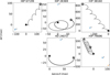 |
Fig. D.1 Proper motion test for the five stellar companion candidates with multiple epochs. As in Figure 4, a filled star indicates the displacement expected for a bound source with no relative motion to the star, whereas an empty star marks the location of a static background source. Second epochs are labeled by a ‘2’, third epochs by a ‘3’. The large deviations from the filled star are likely caused by orbital motion. |
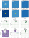 |
Fig. D.2 Upper panel: flux maps (in contrast units) showing the stellar companion candidates detected with cADI. Lower panel: GaiaPMEX (sma, mass) maps, with contours outlining the area corresponding to the 68% and 95% confidence level. Photometric masses (dots) or lower limits (arrows) are overplotted for comparison. The HD 74341B map should be interpreted as a nondetection, the white area being incompatible with the absence of a signal. |
Appendix E Effect of input assumptions on occurrence rates
We explored the dependence of the results derived in Section 3 on several input assumptions: the uncertainty on stellar age, the choice of the substellar evolutionary model, the degree of disequilibrium chemistry of planet atmospheres. In principle, all of them are expected to induce systematic deviations in the luminosity-mass relation, possibly impacting the reliability of the derived occurrence rates.
As a first step, we evaluated the impact of model selection by repeating the computations from Table 3 using the AMES-Cond models (Baraffe et al. 2003) and the Sonora Bobcat models (Marley et al. 2021). AMES-Cond models ignore the effect of dust opacity and are therefore more appropriate for objects with Teff ≲ 1300 K compared to fully dusty models such as the AMES-Dusty models (Baraffe et al. 2003). The derived completeness maps are shown on the left side of Figure E.1; the differences between completeness values are plotted on the right side. In this regard, we stress that, given that it is the mean detection probability across the (mass, sma) area 𝒜 that enters into Eq. 2, absolute differences are a more accurate proxy than relative differences when evaluating the impact of completeness maps variations on the derived frequency posteriors. Inspection of Figure E.1 clearly indicates that the discrepancies are the widest in the mass range [1, 5] MJup, and rapidly decrease at larger masses: this can be seen as a consequence of the stronger cooling rate of less massive objects, combined with the larger theoretical uncertainties at lower masses.
As a consequence of this observation, we expect the lower mass value selected to define 𝒜, Mlow to have a large impact on the accuracy of the results. We quantified this effect by computing occurrence rates under the three models for Mlow = [1,2,3,4,5] MJup. As expected, the problem exacerbates for lower values of Mlow (Figure E.2). This test justifies our conservative choice for 𝒜 (Sec. 3.4).
Afterwards, we investigated the dependence of the results on the assumption of chemical equilibrium: in particular, we used two suites of ATMO models that assume 1) chemical equilibrium (ATMO-CEQ) or 2) strong chemical disequilibrium (ATMO-NEQ-S), that is, a different relation for the vertical mixing coefficient (Phillips et al. 2020). Given a certain H-band magnitude, the fractional mass difference, computed as a function of age and ATMO-NEQ-W mass (m ∈ [1,10] MJup), can be as large as 30% compared to the chemical equilibrium case. The variation is larger at lower masses and larger ages, that is, at lower effective temperatures. The derived completeness maps, analogous to Figure E.1, are shown in Figure E.3. Given our careful choice of mass boundaries, it is possible to argue that completeness values within 𝒜 are dominated by projection effects rather than detection limits. Hence, we expect the occurrence rates to be fully consistent with those of the original analysis.
Finally, we provide similar completeness maps to quantify the dependence on age uncertainty: Figure E.4 shows the variation of the maps when assuming lower and upper values for stellar ages.
All the occurrence rates derived in this Section are visually compared in Figure E.5. It is evident that any doublet of estimates is compatible within the errors, making the estimates presented in this work robust against systematic effects.
 |
Fig. E.1 Effect of model selection on survey completeness: maps assuming the Ames-COND model (top row) and the Sonora model (bottom row). Left panels show completeness maps, while right panels indicate the difference relative to the map used for the analysis. The green dashed box indicates our nominal choice of 𝒜. |
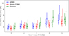 |
Fig. E.2 Trend of the uncertainties in the derived occurrence rates with Mlow. Each model - shown as a triplet (nominal ages, lower ages, upper ages) – is plotted in a different color. Horizontal offsets have been applied to each line for the sake of visualization. |
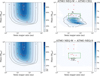 |
Fig. E.3 Effect of non-equilibrium chemistry on survey completeness: maps using the ATMO models assuming equilibrium chemistry (top row) and strong disequilibrium chemistry (bottom row). Left panels show completeness maps, while right panels indicate the difference relative to the map used for the analysis. The green dashed box indicates our nominal choice of 𝒜. |
 |
Fig. E.4 Effect of age uncertainty on survey completeness: maps assuming lower (top row) and upper (bottom row) values for stellar ages. Left panels show completeness maps, while right panels indicate the difference relative to the map used for the analysis. The green dashed box indicates our nominal choice of 𝒜. |
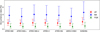 |
Fig. E.5 Effect of model selection and age uncertainty on planet occurrence (𝒜 = [5,13] MJup × [10,100] au): results for the entire sample (red squares), the BA subsample (blue diamonds), the FGK subsample (green circles) using: the standard ATMO-NEQ-weak model (ATMO-NW); the same model with lower (ATMO-NW, L) and upper (ATMO-NW, U) ages; the ATMO model with no (ATMO-C) and strong (ATMO-NS) disequilibrium chemistry; the AMES-Cond model (AMES-COND) and the Sonora Bobcat model (SONORA). A Jeffreys prior is assumed (see Section 3.4). |
References
- Allard, F., Homeier, D., & Freytag, B. 2011, ASP Conf. Ser., 448, 91 [Google Scholar]
- Astropy Collaboration (Robitaille, T. P., et al.) 2013, A&A, 558, A33 [NASA ADS] [CrossRef] [EDP Sciences] [Google Scholar]
- Baraffe, I., Chabrier, G., Barman, T. S., Allard, F., & Hauschildt, P. H. 2003, A&A, 402, 701 [NASA ADS] [CrossRef] [EDP Sciences] [Google Scholar]
- Baratella, M., D’Orazi, V., Carraro, G., et al. 2020, A&A, 634, A34 [NASA ADS] [CrossRef] [EDP Sciences] [Google Scholar]
- Baxter, C., Désert, J.-M., Tsai, S.-M., et al. 2021, A&A, 648, A127 [NASA ADS] [CrossRef] [EDP Sciences] [Google Scholar]
- Bell, C. P. M., Mamajek, E. E., & Naylor, T. 2015, MNRAS, 454, 593 [Google Scholar]
- Beuzit, J. L., Vigan, A., Mouillet, D., et al. 2019, A&A, 631, A155 [NASA ADS] [CrossRef] [EDP Sciences] [Google Scholar]
- Biazzo, K., D’Orazi, V., Desidera, S., et al. 2012, MNRAS, 427, 2905 [NASA ADS] [CrossRef] [Google Scholar]
- Biazzo, K., Bozza, V., Mancini, L., & Sozzetti, A. 2022, Astrophys. Space Sci. Lib., 466, 3 [NASA ADS] [CrossRef] [Google Scholar]
- Boccaletti, A., Chauvin, G., Wildi, F., et al. 2022, SPIE Conf. Ser., 12184, 121841S [NASA ADS] [Google Scholar]
- Bonavita, M. 2020, Astrophysics Source Code Library [record ascl:2010.008] [Google Scholar]
- Bonavita, M., Gratton, R., Desidera, S., et al. 2022, A&A, 663, A144 [NASA ADS] [CrossRef] [EDP Sciences] [Google Scholar]
- Bonnefoy, M., Perraut, K., Lagrange, A. M., et al. 2018, A&A, 618, A63 [NASA ADS] [CrossRef] [EDP Sciences] [Google Scholar]
- Boss, A. P. 1997, Science, 276, 1836 [Google Scholar]
- Bourrier, V., Dumusque, X., Dorn, C., et al. 2018, A&A, 619, A1 [NASA ADS] [CrossRef] [EDP Sciences] [Google Scholar]
- Bowler, B. P. 2016, PASP, 128, 102001 [Google Scholar]
- Bowler, B. P., & Nielsen, E. L. 2018, in Handbook of Exoplanets, eds. H. J. Deeg, & J. A. Belmonte (Berlin: Springer), 155 [Google Scholar]
- Bowler, B. P., Liu, M. C., Shkolnik, E. L., & Tamura, M. 2015, ApJS, 216, 7 [Google Scholar]
- Bowler, B. P., Blunt, S. C., & Nielsen, E. L. 2020, AJ, 159, 63 [Google Scholar]
- Brandt, G. M., Brandt, T. D., Dupuy, T. J., Michalik, D., & Marleau, G.-D. 2021, ApJ, 915, L16 [NASA ADS] [CrossRef] [Google Scholar]
- Bryan, M. L., Knutson, H. A., Howard, A. W., et al. 2016, ApJ, 821, 89 [NASA ADS] [CrossRef] [Google Scholar]
- Chabrier, G., Johansen, A., Janson, M., & Rafikov, R. 2014, in Protostars and Planets VI, eds. H. Beuther, R. S. Klessen, C. P. Dullemond, & T. Henning (Tucson: University of Arizona Press), 619 [Google Scholar]
- Chabrier, G., Baraffe, I., Phillips, M., & Debras, F. 2023, A&A, 671, A119 [NASA ADS] [CrossRef] [EDP Sciences] [Google Scholar]
- Charnay, B., Bézard, B., & Baudino, J.-L. 2019, EPSC-DPS Joint Meeting, 2019, 1450 [Google Scholar]
- Chauvin, G., Lagrange, A. M., Dumas, C., et al. 2004, A&A, 425, L29 [NASA ADS] [CrossRef] [EDP Sciences] [Google Scholar]
- Chauvin, G., Desidera, S., Lagrange, A. M., et al. 2017, in SF2A-2017: Proceedings of the Annual meeting of the French Society of Astronomy and Astrophysics, eds. C. Reylé, P. Di Matteo, F. Herpin, et al. [Google Scholar]
- Chilcote, J. K., Bailey, V. P., De Rosa, R., et al. 2018, SPIE Conf. Ser., 10702, 1070244 [NASA ADS] [Google Scholar]
- Chilcote, J., Konopacky, Q., De Rosa, R. J., et al. 2020, SPIE Conf. Ser., 11447, 114471S [NASA ADS] [Google Scholar]
- Chomez, A., Lagrange, A. M., Delorme, P., et al. 2023, A&A, 675, A205 [NASA ADS] [CrossRef] [EDP Sciences] [Google Scholar]
- Chomez, A., Delorme, P., & Lagrange, A.-M. 2024, A&A, submitted [Google Scholar]
- Courtney-Barrer, B., De Rosa, R., Kokotanekova, R., et al. 2023, A&A, 680, A34 [NASA ADS] [CrossRef] [EDP Sciences] [Google Scholar]
- Covino, E., Esposito, M., Barbieri, M., et al. 2013, A&A, 554, A28 [NASA ADS] [CrossRef] [EDP Sciences] [Google Scholar]
- Cumming, A., Butler, R. P., Marcy, G. W., et al. 2008, PASP, 120, 531 [CrossRef] [Google Scholar]
- Currie, T., Marois, C., Cieza, L., et al. 2019, ApJ, 877, L3 [Google Scholar]
- Currie, T., Biller, B., Lagrange, A., et al. 2023, ASP Conf. Ser., 534, 799 [NASA ADS] [Google Scholar]
- Delorme, P., Meunier, N., Albert, D., et al. 2017, in SF2A-2017: Proceedings of the Annual meeting of the French Society of Astronomy and Astrophysics, eds. C. Reylé, P. Di Matteo, F. Herpin, E. Lagadec, A. Lançon, Z. Meliani, & F. Royer, Di [Google Scholar]
- Desidera, S., Chauvin, G., Bonavita, M., et al. 2021, A&A, 651, A70 [EDP Sciences] [Google Scholar]
- Desidera, S., Squicciarini, V., & Brandner, W. 2024, A&A, in prep. [Google Scholar]
- De Rosa, R. J., Nguyen, M. M., Chilcote, J., et al. 2020a, J. Astron. Teles. Instrum. Syst., 6, 015006 [CrossRef] [Google Scholar]
- De Rosa, R. J., Nielsen, E. L., Wang, J. J., et al. 2020b, AJ, 159, 1 [Google Scholar]
- De Rosa, R. J., Nielsen, E. L., Wahhaj, Z., et al. 2023, A&A, 672, A94 [NASA ADS] [CrossRef] [EDP Sciences] [Google Scholar]
- de Zeeuw, P. T., Hoogerwerf, R., de Bruijne, J. H. J., Brown, A. G. A., & Blaauw, A. 1999, AJ, 117, 354 [Google Scholar]
- Dohlen, K., Langlois, M., Saisse, M., et al. 2008, SPIE Conf. Ser., 7014, 70143L [Google Scholar]
- D’Orazi, V., Biazzo, K., & Randich, S. 2011, A&A, 526, A103 [NASA ADS] [CrossRef] [EDP Sciences] [Google Scholar]
- Draper, Z. H., Marois, C., Wolff, S., et al. 2014, SPIE Conf. Ser., 9147, 91474Z [NASA ADS] [Google Scholar]
- Dulz, S. D., Plavchan, P., Crepp, J. R., et al. 2020, ApJ, 893, 122 [NASA ADS] [CrossRef] [Google Scholar]
- Elliott, A., Boyajian, T., Ellis, T., et al. 2024, PASA, 41, e043 [NASA ADS] [CrossRef] [Google Scholar]
- Flasseur, O., Denis, L., Thiébaut, É., & Langlois, M. 2018, A&A, 618, A138 [NASA ADS] [CrossRef] [EDP Sciences] [Google Scholar]
- Flasseur, O., Denis, L., Thiébaut, É., & Langlois, M. 2020a, A&A, 637, A9 [NASA ADS] [CrossRef] [EDP Sciences] [Google Scholar]
- Flasseur, O., Denis, L., Thiébaut, É., & Langlois, M. 2020b, A&A, 634, A2 [Google Scholar]
- Franson, K., & Bowler, B. P. 2023, AJ, 165, 246 [NASA ADS] [CrossRef] [Google Scholar]
- Franson, K., Bowler, B. P., Brandt, T. D., et al. 2022, AJ, 163, 50 [NASA ADS] [CrossRef] [Google Scholar]
- Franson, K., Bowler, B. P., Zhou, Y., et al. 2023, ApJ, 950, L19 [NASA ADS] [CrossRef] [Google Scholar]
- Gagné, J., Faherty, J. K., & Mamajek, E. E. 2018a, ApJ, 865, 136 [Google Scholar]
- Gagné, J., Mamajek, E. E., Malo, L., et al. 2018b, ApJ, 856, 23 [Google Scholar]
- Gaia Collaboration (Vallenari, A., et al.) 2023, A&A, 674, A1 [NASA ADS] [CrossRef] [EDP Sciences] [Google Scholar]
- Galicher, R., & Mazoyer, J. 2024, Comptes Rendus Physique, 24, 133 [Google Scholar]
- Galicher, R., Marois, C., Macintosh, B., et al. 2016, A&A, 594, A63 [NASA ADS] [CrossRef] [EDP Sciences] [Google Scholar]
- Gandolfi, D., Barragán, O., Hatzes, A. P., et al. 2017, AJ, 154, 123 [NASA ADS] [CrossRef] [Google Scholar]
- Gaudi, B. S., Meyer, M., & Christiansen, J. 2021, in ExoFrontiers; Big Questions in Exoplanetary Science, ed. N. Madhusudhan (Oxford: IOP Publishing Ltd), 2 [Google Scholar]
- Ginsburg, A., Sipocz, B. M., Brasseur, C. E., et al. 2019, AJ, 157, 98 [NASA ADS] [CrossRef] [Google Scholar]
- Gratton, R., Mesa, D., Bonavita, M., et al. 2023, Nat. Commun., 14, 6232 [Google Scholar]
- Gratton, R., Bonavita, M., Mesa, D., et al. 2024, A&A, 685, A119 [NASA ADS] [CrossRef] [EDP Sciences] [Google Scholar]
- Harris, C. R., Millman, K. J., van der Walt, S. J., et al. 2020, Nature, 585, 357 [NASA ADS] [CrossRef] [Google Scholar]
- Hinkley, S., Lacour, S., Marleau, G. D., et al. 2023, A&A, 671, L5 [NASA ADS] [CrossRef] [EDP Sciences] [Google Scholar]
- Janson, M., Squicciarini, V., Delorme, P., et al. 2021, A&A, 646, A164 [NASA ADS] [CrossRef] [EDP Sciences] [Google Scholar]
- Kasdin, N. J., Bailey, V. P., Mennesson, B., et al. 2020, SPIE Conf. Ser., 11443, 114431U [Google Scholar]
- Kasper, M., Cerpa Urra, N., Pathak, P., et al. 2021, The Messenger, 182, 38 [Google Scholar]
- Keppler, M., Benisty, M., Müller, A., et al. 2018, A&A, 617, A44 [NASA ADS] [CrossRef] [EDP Sciences] [Google Scholar]
- Kervella, P., Arenou, F., Mignard, F., & Thévenin, F. 2019, A&A, 623, A72 [NASA ADS] [CrossRef] [EDP Sciences] [Google Scholar]
- Kervella, P., Arenou, F., & Thévenin, F. 2022, A&A, 657, A7 [NASA ADS] [CrossRef] [EDP Sciences] [Google Scholar]
- Kiefer, F., Lagrange, A.-M., Rubini, P., & Philipot, F. 2024, arXiv e-prints [arXiv:2409.16992] [Google Scholar]
- Konopacky, Q. M., Rameau, J., Duchêne, G., et al. 2016, ApJ, 829, L4 [Google Scholar]
- Kuzuhara, M., Currie, T., Takarada, T., et al. 2022, ApJ, 934, L18 [NASA ADS] [CrossRef] [Google Scholar]
- Lacedelli, G., Malavolta, L., Borsato, L., et al. 2021, MNRAS, 501, 4148 [NASA ADS] [CrossRef] [Google Scholar]
- Lacour, S., Wang, J. J., Rodet, L., et al. 2021, A&A, 654, L2 [NASA ADS] [CrossRef] [EDP Sciences] [Google Scholar]
- Lafrenière, D., Doyon, R., Marois, C., et al. 2007, ApJ, 670, 1367 [Google Scholar]
- Lagrange, A. M., Gratadour, D., Chauvin, G., et al. 2009, A&A, 493, L21 [NASA ADS] [CrossRef] [EDP Sciences] [Google Scholar]
- Lagrange, A. M., Philipot, F., Rubini, P., et al. 2023, A&A, 677, A71 [NASA ADS] [CrossRef] [EDP Sciences] [Google Scholar]
- Langlois, M., Gratton, R., Lagrange, A. M., et al. 2021, A&A, 651, A71 [NASA ADS] [CrossRef] [EDP Sciences] [Google Scholar]
- Lannier, J., Delorme, P., Lagrange, A. M., et al. 2016, A&A, 596, A83 [NASA ADS] [CrossRef] [EDP Sciences] [Google Scholar]
- Launhardt, R., Henning, T., Quirrenbach, A., et al. 2020, A&A, 635, A162 [NASA ADS] [CrossRef] [EDP Sciences] [Google Scholar]
- Leggett, S. K., Morley, C. V., Marley, M. S., & Saumon, D. 2015, ApJ, 799, 37 [NASA ADS] [CrossRef] [Google Scholar]
- Leggett, S. K., Tremblin, P., Esplin, T. L., Luhman, K. L., & Morley, C. V. 2017, ApJ, 842, 118 [NASA ADS] [CrossRef] [Google Scholar]
- Leike, R. H., Glatzle, M., & Enßlin, T. A. 2020, A&A, 639, A138 [NASA ADS] [CrossRef] [EDP Sciences] [Google Scholar]
- Lindegren, L., Klioner, S. A., Hernández, J., et al. 2021, A&A, 649, A2 [EDP Sciences] [Google Scholar]
- Liu, M. C., Wahhaj, Z., Biller, B. A., et al. 2010, SPIE Conf. Ser., 7736, 77361K [Google Scholar]
- Macintosh, B. A., Anthony, A., Atwood, J., et al. 2014a, SPIE, 9148, 152 [Google Scholar]
- Macintosh, B., Graham, J. R., Ingraham, P., et al. 2014b, Proc. Natl. Acad. Sci., 111, 12661 [NASA ADS] [CrossRef] [Google Scholar]
- Macintosh, B., Graham, J. R., Barman, T., et al. 2015, Science, 350, 64 [Google Scholar]
- Magrini, L., Viscasillas Vázquez, C., Spina, L., et al. 2023, A&A, 669, A119 [NASA ADS] [CrossRef] [EDP Sciences] [Google Scholar]
- Maire, J., Ingraham, P. J., De Rosa, R. J., et al. 2014, SPIE Conf. Ser., 9147, 914785 [NASA ADS] [Google Scholar]
- Marley, M. S., Saumon, D., Visscher, C., et al. 2021, ApJ, 920, 85 [NASA ADS] [CrossRef] [Google Scholar]
- Marois, C., Lafrenière, D., Doyon, R., Macintosh, B., & Nadeau, D. 2006, ApJ, 641, 556 [Google Scholar]
- Marois, C., Macintosh, B., Barman, T., et al. 2008, Science, 322, 1348 [Google Scholar]
- McBride, J., Graham, J. R., Macintosh, B., et al. 2011, PASP, 123, 692 [NASA ADS] [CrossRef] [Google Scholar]
- Mesa, D., Gratton, R., Kervella, P., et al. 2023, A&A, 672, A93 [NASA ADS] [CrossRef] [EDP Sciences] [Google Scholar]
- Miles, B. E., Skemer, A. J. I., Morley, C. V., et al. 2020, AJ, 160, 63 [NASA ADS] [CrossRef] [Google Scholar]
- Mordasini, C., Alibert, Y., & Benz, W. 2009, A&A, 501, 1139 [CrossRef] [EDP Sciences] [Google Scholar]
- Murphy, S. J., Lawson, W. A., & Bessell, M. S. 2013, MNRAS, 435, 1325 [Google Scholar]
- Musielak, Z. E., Cuntz, M., Marshall, E. A., & Stuit, T. D. 2005, A&A, 434, 355 [NASA ADS] [CrossRef] [EDP Sciences] [Google Scholar]
- Nguyen, C. T., Costa, G., Girardi, L., et al. 2022, A&A, 665, A126 [NASA ADS] [CrossRef] [EDP Sciences] [Google Scholar]
- Nielsen, E. L., Liu, M. C., Wahhaj, Z., et al. 2013, ApJ, 776, 4 [Google Scholar]
- Nielsen, E. L., De Rosa, R. J., Macintosh, B., et al. 2019, AJ, 158, 13 [Google Scholar]
- Ochsenbein, F., Bauer, P., & Marcout, J. 2000, A&AS, 143, 23 [NASA ADS] [CrossRef] [EDP Sciences] [Google Scholar]
- Pecaut, M. J., & Mamajek, E. E. 2016, MNRAS, 461, 794 [Google Scholar]
- Perrin, M. D., Maire, J., Ingraham, P., et al. 2014, SPIE Conf. Ser., 9147, 91473J [NASA ADS] [Google Scholar]
- Perrin, M. D., Ingraham, P., Follette, K. B., et al. 2016, SPIE Con. Ser., 9908, 990837 [NASA ADS] [Google Scholar]
- Philipot, F., Lagrange, A. M., Rubini, P., Kiefer, F., & Chomez, A. 2023, A&A, 670, A65 [NASA ADS] [CrossRef] [EDP Sciences] [Google Scholar]
- Phillips, M. W., Tremblin, P., Baraffe, I., et al. 2020, A&A, 637, A38 [NASA ADS] [CrossRef] [EDP Sciences] [Google Scholar]
- Pollack, J. B., Hubickyj, O., Bodenheimer, P., et al. 1996, Icarus, 124, 62 [NASA ADS] [CrossRef] [Google Scholar]
- Poyneer, L. A., Palmer, D. W., Macintosh, B., et al. 2016, Appl. Opt., 55, 323 [NASA ADS] [CrossRef] [Google Scholar]
- Rameau, J., Chauvin, G., Lagrange, A. M., et al. 2013, A&A, 553, A60 [NASA ADS] [CrossRef] [EDP Sciences] [Google Scholar]
- Rameau, J., Nielsen, E. L., De Rosa, R. J., et al. 2016, ApJ, 822, L29 [Google Scholar]
- Reggiani, M., Meyer, M. R., Chauvin, G., et al. 2016, A&A, 586, A147 [NASA ADS] [CrossRef] [EDP Sciences] [Google Scholar]
- Rogers, L. A. 2015, ApJ, 801, 41 [Google Scholar]
- Rosenthal, L. J., Howard, A. W., Knutson, H. A., & Fulton, B. J. 2024, ApJS, 270, 1 [NASA ADS] [CrossRef] [Google Scholar]
- Ruffio, J.-B., Macintosh, B., Wang, J. J., et al. 2017, ApJ, 842, 14 [Google Scholar]
- Sallum, S., Follette, K. B., Eisner, J. A., et al. 2015, Nature, 527, 342 [Google Scholar]
- Santerne, A., Moutou, C., Tsantaki, M., et al. 2016, A&A, 587, A64 [NASA ADS] [CrossRef] [EDP Sciences] [Google Scholar]
- Skrutskie, M. F., Cutri, R. M., Stiening, R., et al. 2006, AJ, 131, 1163 [NASA ADS] [CrossRef] [Google Scholar]
- Spiegel, D. S., & Burrows, A. 2012, ApJ, 745, 174 [Google Scholar]
- Squicciarini, V., & Bonavita, M. 2022, A&A, 666, A15 [NASA ADS] [CrossRef] [EDP Sciences] [Google Scholar]
- Stone, J. M., Skemer, A. J., Hinz, P. M., et al. 2018, AJ, 156, 286 [Google Scholar]
- Tran, D., Konopacky, Q., & GPIES Collaboration 2016, AAS Meeting Abstracts, 228, 120.01 [Google Scholar]
- Uyama, T., Hashimoto, J., Kuzuhara, M., et al. 2017, AJ, 153, 106 [Google Scholar]
- Vigan, A., Fontanive, C., Meyer, M., et al. 2021, A&A, 651, A72 [EDP Sciences] [Google Scholar]
- Vorobyov, E. I. 2013, A&A, 552, A129 [NASA ADS] [CrossRef] [EDP Sciences] [Google Scholar]
- Waisberg, I., Klein, Y., & Katz, B. 2023a, Res. Notes Am. Astron. Soc., 7, 125 [Google Scholar]
- Waisberg, I., Klein, Y., & Katz, B. 2023b, Res. Notes Am. Astron. Soc., 7, 78 [Google Scholar]
- Wang, J. J., Rajan, A., Graham, J. R., et al. 2014, SPIE Conf. Ser., 9147, 914755 [NASA ADS] [Google Scholar]
- Wang, J. J., Ruffio, J.-B., De Rosa, R. J., et al. 2015, Astrophysics Source Code Library [record ascl:1506.001] [Google Scholar]
- Wang, J. J., Perrin, M. D., Savransky, D., et al. 2018, J. Astron. Teles. Instrum. Syst., 4, 018002 [NASA ADS] [Google Scholar]
- Wolff, S. G., Perrin, M. D., Maire, J., et al. 2014, SPIE Conf. Ser., 9147, 91477H [NASA ADS] [Google Scholar]
- Wolthoff, V., Reffert, S., Quirrenbach, A., et al. 2022, A&A, 661, A63 [NASA ADS] [CrossRef] [EDP Sciences] [Google Scholar]
- Wright, E. L., Eisenhardt, P. R. M., Mainzer, A. K., et al. 2010, AJ, 140, 1868 [Google Scholar]
- Zhang, S. Y., Duchêne, G., De Rosa, R. J., et al. 2023, AJ, 165, 219 [Google Scholar]
- Zhu, W., & Wu, Y. 2018, AJ, 156, 92 [Google Scholar]
- Zuckerman, B. 2019, ApJ, 870, 27 [Google Scholar]
- Zuckerman, B., Song, I., Bessell, M. S., & Webb, R. A. 2001, ApJ, 562, L87 [NASA ADS] [CrossRef] [Google Scholar]
- Zuckerman, B., Bessell, M. S., Song, I., & Kim, S. 2006, ApJ, 649, L115 [NASA ADS] [CrossRef] [Google Scholar]
- Zuckerman, B., Rhee, J. H., Song, I., & Bessell, M. S. 2011, ApJ, 732, 61 [Google Scholar]
- Zurlo, A. 2024, arXiv e-prints [arXiv:2404.05797] [Google Scholar]
- Zurlo, A., Gozdziewski, K., Lazzoni, C., et al. 2022, A&A, 666, A133 [NASA ADS] [CrossRef] [EDP Sciences] [Google Scholar]
Empirically estimated based on the Extrasolar Planet Encyclopaedia: http://www.exoplanet.eu/
We could not retrieve science commissioning data from 2014 from the old Gemini website (Macintosh et al. 2014a). However, the targeted stars were only known hosts of exoplanets or disks (HR 8799, HR 4796, HD 95806) that were later re-observed during GPIES.
The distribution of ∆PA across the database shows a bump for ∆PA > 12. Whereas just 12 sequences have 10° < ∆PA ≤ 12°, 49 observations are found inside the 12° < ∆PA ≤ 14° bin.
Unlike SPHERE, no PSF exposure is taken before and/or after the scientific observation in GPI.
Input contrast spectra, created using the same procedure as spectral priors, are arbitrarily defined using the following parameters: (Teff, log 𝑔, Z/Z⊙, CO) = (1000 K, 4.0,1.0,0.5) for the T type and (Teff, log 𝑔, Z/Z⊙, CO) = (1900 K, 3.0,10.0,0.6) for the L type.
The library, available at http://svo2.cab.inta-csic.es/theory/newov2/index.php?models=bt-nextցen-aցss2009, is defined by the following astrophysical parameters: log 𝑔[cm s−2] = 4.5, log Z/Z⊙ = 0, alpha enhancement = 0.
The status of all cADI candidates but one could be confirmed through dynamical arguments; the remaining one is too bright to allow for the CMD test.
The correlation between S/N maps under any two spectral priors is larger than zero. By “number of effectively independent spectral priors” we mean the ratio Npositives,20priors/Npositives,1priors, estimated through extensive testing.
Using the most recent version, that features a new equation of state for dense hydrogen-helium mixtures: https://noctis.erc-atmo.eu/fsdownload/zyU96xA6o/phillips2020
The amount of vertical mixing in disequilibrium models is parametrized through the eddy diffusion coefficient KZZ. Constraining KZZ is a long-standing issue (see discussion in Phillips et al. 2020).
The no-ADI algorithm can be thought as a cADI but with no median-subtraction step. The advantage of the method is to avoid selfsubtraction of signal from the source, a problem becoming more severe at shorter separations; on the other hand, this is obtained at the price of much poorer detection limits.
All Tables
Occurrence rates for different definitions of the (mass, sma) range 𝒜 and for the two choices for the prior distribution (U: uniform; J: Jeffreys). (a)95% upper limit.
Stellar properties for the sample considered in this work. The full table is available in electronic form at the CDS.
Observing log for the observations considered in this work. The full table is available in electronic form on Zenodo.
Companion candidates detected in this work. The full table is available in electronic form at the CDS.
Stellar companions identified in the sample with their astrometric and photometric properties. In addition to GPI measurements, literature astrometry is reported too. The table is also available in electronic form at the CDS.
All Figures
|
Fig. 1 Age of the final stellar sample as a function of distance. The color scale labels different spectral types. Kernel density estimates for the distribution of the two properties are provided on top and to the right of the main plot. |
| In the text | |
|
Fig. 2 5σ detection limits obtained with PACO. Individual curves are plotted in gray. The median curve is plotted as a light blue solid line, the dashed lines representing the 16 and 84% percentiles of the curve distribution. The orange and green solid lines indicate the median detection limits assuming a T-type and an L-type spectral prior, respectively. The gray box marks the inner working angle of the coronagraphic mask. |
| In the text | |
|
Fig. 3 Comparison between PACO and cADI performances. Sources only detected by PACO are shown as blue circles, while sources only seen through cADI are indicated as red diamonds. Common sources are plotted as blue squares with a red edge. |
| In the text | |
|
Fig. 4 Example of proper motion diagram. The astrometric displacement of the candidate around HD 8433OB between the first and the second epoch is compatible with a background source with null motion (empty star). A bound object would have been in a position close to that marked by the filled star and within the boundaries allowed by a Keplerian motion. |
| In the text | |
|
Fig. 5 CMD of the companion candidates detected in this work. Over-plotted to known substellar objects (white squares), background stars are represented as yellow stars if identified through proper motion analysis, or as blue circles if recognized via their color. Ambiguous sources are marked as red crosses. The exclusion area (gray) is defined by the two dashed lines. The two promising candidates (from left to right: C1 (HD 24072), C2 (HIP 78663)) are indicated as red dots. |
| In the text | |
|
Fig. 6 PACO or cADI detection maps for the substellar companions detected in the survey (indicated by arrows). PACO maps are to be read as S/N maps, sharing a common colorbar. Individual colorbars are shown below the two cADI maps. |
| In the text | |
|
Fig. 7 Survey completeness as a function of companion mass and semi-major axis, computed using the ATMO-NEQ-W models. Red stars indicate known substellar companions (see Table 1). |
| In the text | |
|
Fig. 8 Comparison of the survey completeness between N19 (dashed lines) and this work (solid lines). Only the observations used by N19 were used to draw this plot. |
| In the text | |
|
Fig. 9 Occurrence frequency of GP (upper panel) and GP+BD (lower panel) from the re-analysis of the 400-star GPIES sample presented in this work. Aggregated results are shown in blue, whereas results for the BA and the FGK subsample are plotted in green and orange, respectively. The colored area encompasses the [16th, 84th] of the posterior distribution. |
| In the text | |
|
Fig. 10 Comparison of the occurrence rates (left panel: 𝒜 = [2,13] MJup × [3,100] au; right panel: 𝒜 = [5,13] MJup × [10,100] au) of giant planets with previous analyses by Bowler (2016), Nielsen et al. (2019) and Vigan et al. (2021). The left and the right half of each panel are relative to BA and FGK stars, respectively. Estimates indicated by arrows are to be read as 95% upper limits, while error bars on point estimates are defined as to encompass the 68% C.I.. Question marks indicate missing data points. |
| In the text | |
|
Fig. D.1 Proper motion test for the five stellar companion candidates with multiple epochs. As in Figure 4, a filled star indicates the displacement expected for a bound source with no relative motion to the star, whereas an empty star marks the location of a static background source. Second epochs are labeled by a ‘2’, third epochs by a ‘3’. The large deviations from the filled star are likely caused by orbital motion. |
| In the text | |
|
Fig. D.2 Upper panel: flux maps (in contrast units) showing the stellar companion candidates detected with cADI. Lower panel: GaiaPMEX (sma, mass) maps, with contours outlining the area corresponding to the 68% and 95% confidence level. Photometric masses (dots) or lower limits (arrows) are overplotted for comparison. The HD 74341B map should be interpreted as a nondetection, the white area being incompatible with the absence of a signal. |
| In the text | |
|
Fig. E.1 Effect of model selection on survey completeness: maps assuming the Ames-COND model (top row) and the Sonora model (bottom row). Left panels show completeness maps, while right panels indicate the difference relative to the map used for the analysis. The green dashed box indicates our nominal choice of 𝒜. |
| In the text | |
|
Fig. E.2 Trend of the uncertainties in the derived occurrence rates with Mlow. Each model - shown as a triplet (nominal ages, lower ages, upper ages) – is plotted in a different color. Horizontal offsets have been applied to each line for the sake of visualization. |
| In the text | |
|
Fig. E.3 Effect of non-equilibrium chemistry on survey completeness: maps using the ATMO models assuming equilibrium chemistry (top row) and strong disequilibrium chemistry (bottom row). Left panels show completeness maps, while right panels indicate the difference relative to the map used for the analysis. The green dashed box indicates our nominal choice of 𝒜. |
| In the text | |
|
Fig. E.4 Effect of age uncertainty on survey completeness: maps assuming lower (top row) and upper (bottom row) values for stellar ages. Left panels show completeness maps, while right panels indicate the difference relative to the map used for the analysis. The green dashed box indicates our nominal choice of 𝒜. |
| In the text | |
|
Fig. E.5 Effect of model selection and age uncertainty on planet occurrence (𝒜 = [5,13] MJup × [10,100] au): results for the entire sample (red squares), the BA subsample (blue diamonds), the FGK subsample (green circles) using: the standard ATMO-NEQ-weak model (ATMO-NW); the same model with lower (ATMO-NW, L) and upper (ATMO-NW, U) ages; the ATMO model with no (ATMO-C) and strong (ATMO-NS) disequilibrium chemistry; the AMES-Cond model (AMES-COND) and the Sonora Bobcat model (SONORA). A Jeffreys prior is assumed (see Section 3.4). |
| In the text | |
Current usage metrics show cumulative count of Article Views (full-text article views including HTML views, PDF and ePub downloads, according to the available data) and Abstracts Views on Vision4Press platform.
Data correspond to usage on the plateform after 2015. The current usage metrics is available 48-96 hours after online publication and is updated daily on week days.
Initial download of the metrics may take a while.