| Issue |
A&A
Volume 692, December 2024
|
|
|---|---|---|
| Article Number | A263 | |
| Number of page(s) | 17 | |
| Section | Planets, planetary systems, and small bodies | |
| DOI | https://doi.org/10.1051/0004-6361/202451461 | |
| Published online | 18 December 2024 | |
Population of giant planets around B stars from the first part of the BEAST survey★
1
Univ. Grenoble Alpes, CNRS, IPAG,
38000
Grenoble,
France
2
LESIA, Observatoire de Paris, Université PSL, CNRS,
5 Place Jules Janssen,
92190
Meudon,
France
3
INAF – Osservatorio Astronomico di Padova ;
Vicolo dell’Osservatorio 5,
35122
Padova,
Italy
4
Institutionen för astronomi, Stockholms universitet; AlbaNova universitetscentrum,
106 91
Stockholm,
Sweden
5
Centre de Recherche Astrophysique de Lyon (CRAL) UMR 5574, CNRS,
Univ. de Lyon, Univ. Claude Bernard Lyon 1, ENS de Lyon,
69230
Saint-Genis-Laval,
France
6
Physikalisches Institut, Universität Bern,
Gesellschaftsstr. 6,
3012
Bern,
Switzerland
7
Université Côte d’Azur, OCA, CNRS, UMR Lagrange,
06304
Nice,
France
8
Max-Planck-Institut für Astronomie,
Königstuhl 17,
69117
Heidelberg,
Germany
9
Fakultät für Physik, Universität Duisburg-Essen,
Lotharstraße 1,
47057
Duisburg,
Germany
10
Institüt für Astronomie und Astrophysik, Universität Tübingen,
Auf der Morgenstelle 10,
72076
Tübingen,
Germany
11
Department of Astronomy, University of Michigan; 1085 S. University Ave,
Ann Arbor
MI
48109,
USA
12
Landessternwarte, Zentrum für Astronomie der Universität Heidelberg,
Königstuhl 12,
69117
Heidelberg,
Germany
13
University of Zurich, Department of Astrophysics, Winterthurerstr.
190 8057
Zurich,
Switzerland
14
Trottier Institute for Research on Exoplanets, Université de Montréal, Montréal,
H3C 3J7
Québec,
Canada
15
Leiden Observatory, Leiden University,
Leiden,
The Netherlands
16
Scottish Universities Physics Alliance, Institute for Astronomy, University of Edinburgh, Royal Observatory,
Blackford Hill,
Edinburgh
EH9 3HJ,
UK
17
Aix-Marseille Univ., CNRS, CNES, LAM,
Marseille,
France
★★ Corresponding author; This email address is being protected from spambots. You need JavaScript enabled to view it.
Received:
11
July
2024
Accepted:
27
September
2024
Abstract
Context. Exoplanets form from circumstellar protoplanetary disks whose fundamental properties (notably their extent, composition, mass, temperature, and lifetime) depend on the host star properties, such as their mass and luminosity. B stars are among the most massive stars and their protoplanetary disks test extreme conditions for exoplanet formation.
Aims. This paper investigates the frequency of giant planet companions around young B stars (median age of 16 Myr) in the Scorpius-Centaurus (Sco-Cen) association, the closest association containing a large population of B stars.
Methods. We systematically searched for massive exoplanets with the high-contrast direct imaging instrument SPHERE using the data from the BEAST survey, which targets a homogeneous sample of young B stars from the wide Sco-Cen association. We derived accurate detection limits in the case of non-detections.
Results. We found evidence in previous papers for two substellar companions around 42 stars. The masses of these companions are straddling the ~13 Jupiter mass deuterium burning limit, but their mass ratio with respect to their host star is close to that of Jupiter. We derived a frequency of such massive planetary-mass companions around B stars of 11−5+7%, accounting for the survey sensitivity.
Conclusions. The discoveries of substellar companions b Centaurib and μ2 Sco B happened after only a few stars in the survey had been observed, raising the possibility that massive Jovian planets might be common around B stars. However, our statistical analysis shows that the occurrence rate of such planets is similar around B stars and around solar-type stars of a similar age, while B-star companions exhibit low mass ratios and a larger semi-major axis.
Key words: methods: statistical / planets and satellites: detection / planets and satellites: formation / stars: massive / planets and satellites: gaseous planets
Based on data obtained with the ESO/VLT SPHERE instrument under programs 1101.C-0258(A/B/C/D).
© The Authors 2024
 Open Access article, published by EDP Sciences, under the terms of the Creative Commons Attribution License (https://creativecommons.org/licenses/by/4.0), which permits unrestricted use, distribution, and reproduction in any medium, provided the original work is properly cited.
This article is published in open access under the Subscribe to Open model. This email address is being protected from spambots. You need JavaScript enabled to view it. to support open access publication.
1 Introduction
Though exoplanets have been found around a wide variety of stellar hosts, notably around very low-mass stars (from Earthmass planets (Gillon et al. 2016, e.g., TRAPPIST b-f) to giants (Chauvin et al. 2004, e.g., 2M1207b)), their presence around stars more massive than a few solar masses has not been thoroughly investigated as of now. Their intrinsic rarity, large radii, masses, strong activity, and scarce emission or absorption line density make them unsuited for radial velocity surveys and poor targets for transit surveys, while their intense brightness offers unfavorable contrast for direct imaging. Reffert et al. (2015), and Wolthoff et al. (2022) have shown from radial velocity surveys of GK giants (which are the evolved counterparts of young A and late-B stars) that short separation giant exoplanets are more frequent with increasing stellar masses up to around 2 M⊙ and then this frequency decreases. The prospects on the theoretical side are not more promising for giant exoplanet formation around massive stars, with the strong UV flux of B-type stars quickly photo-evaporating their protoplanetary disks and thus making such massive stars an unfavorable environment for planet formation by core accretion. The first large direct imaging surveys conducted with the new generation adaptive optics (AO) instruments, SHINE (using SPHERE, Vigan et al. 2021) and GPIES (using GPI, Nielsen et al. 2019), targeted mostly solar-type stars and find that while massive giant planets did exist around such stars they were relatively rare. However, direct imaging has recently shown that massive stars do harbor planetary-mass companions at large separations (Janson et al. 2021a; Squicciarini et al. 2022; Chomez et al. 2023b). Though most of them are very massive (11–15 MJup) in absolute mass, these companions have mass ratios relative to their host stars that are below 0.2%, lower than those of most imaged exoplanets and close to that of Jupiter. Interestingly, these companions have been found at very large separations, hundreds of au from their host stars. Though Squicciarini et al. (2022) show that the expected stellar irradiation of the protoplanetary disk at the present-day separation (≈ 290 au) of μ2 Sco b is similar to that of early Jupiter, the exoplanets discovered by the YSES survey (Bohn et al. 2020, 2021), targeting solar-type stars of the Sco-Cen young association, show that these lower-mass stars do also harbor very large separation giant planets.
The B-star Exoplanet Abundance Study (BEAST) is a direct imaging high-contrast survey with the extreme AO instrument SPHERE, targeting 85 B-type stars in the young Scorpius-Centaurus (Sco-Cen) region with the aim of detecting giant planets at wide separations and constraining their occurrence rate and physical properties. The individual discoveries of b Centauri b and μ2 Sco B, which were achieved during an early stage of the survey (out of the 85 stars observed in the sample, they were the first and seventh ones, respectively), raised the possibility that massive Jovian planets might be relatively common around B stars. However, a dedicated statistical analysis is necessary to confirm or refute such a hypothesis and firmly establish whether large separation planetary-mass companions around massive stars are common or not and whether they are distinct in any way from the population that is known around solar–mass stars.
In this work, we present the statistical analysis of the first half of the survey that already has a complete follow-up of all identified candidates. Numbering 34 stars after the removal of eight outlying objects that did not respect the initial selection criteria, this homogeneous statistical sample is twice as large, and much deeper, than the previous largest direct imaging survey for exoplanets around B stars, the 18-strong sample studied by Janson et al. (2011).
The sample used for this study is described in Sect. 2. Section 3 presents the observations and the data analysis. Section 4 presents the companions identified around the stars of our sample. Section 5 describes the detection limits achieved around these stars to assess the completeness of the survey. Section 6 explores the statistics of the giant planet population as observed by our survey, in addition to the plausible pathways to account for the formation of the companions we detected.
2 Sample description
2.1 Initial BEAST sample
Starting from the census of B-type members of Sco-Cen, defined as those stars with a kinematic membership probability to the association according to Rizzuto et al. (2011), the target list of BEAST was assembled (Janson et al. 2021b, hereafter J21) by considering every B star belonging to Sco-Cen, with no known stellar companion with a separation in the 0.1″−6″ range, no previous deep observations with SPHERE, and declination outside of the −24.6° ± 3.0° range, due to telescope tracking limitations. The final roster of 85 stars, aged between 2 and 27 Myr, spans a wide range of stellar masses [2.4–16]M⊙, corresponding to spectral types from B0 to B9.5.
No prior indications of the possible presence of substellar companions were available at the time of sample definition; additionally, no selection and/or ranking was operated based on a priori estimations of planet detectability. In other words, neither the target selection nor the first-epoch observational strategy is affected by observational biases caused by assumptions on the underlying substellar companion population whose properties we aimed to constrain. The same argument applies to the followup within the standard BEAST program, which follows up on all identified point sources with equal priority, regardless of their estimated properties.
To further ensure the sample studied in this paper is free from observational biases, we decided to strictly adhere to a first-epoch criterion for the selection of the sample. We thus restricted the analysis to the first N stars imaged in the survey, exploiting any additional follow-up epoch regardless of its date. The value of N was optimized to simultaneously 1) allow for an even division of the sample between the intermediate and the final analysis, and 2) to minimize the fraction of stars with only a single epoch. The resulting value of N = 42 corresponds to stars with a first epoch observed no later than April 9, 2021. Only five among those stars have not yet been reobserved to date. Four of them show no candidate companion while the detection limits of the fifth are carefully handled in Sect. 5.1 to ensure statistical consistency.
2.2 Revised stellar host properties
We decided to reassess the main properties (namely age and mass) of the entire BEAST stellar sample compared to the original analysis presented in J21, so as to account for several theoretical as well as observational advancements that occurred in the last few years: (1) the code underlying J21’s analysis is now a robust tool known as MADYS (Squicciarini & Bonavita 2022); (2) a new version of nonrotating, solar-metallicity PARSEC isochrones, covering the full pre-main-sequence (pre-MS) evolution of [0.09, 14] M⊙ stars, is now available (Nguyen et al. 2022); (3) as a consequence of the former, stellar parameters based on the direct isochrone fitting of their photometry could be derived; (4) the astrometric solution for several stars in the sample is significantly improved thanks to Gaia Data Release 3 (DR3) (Gaia Collaboration 2023) compared to the previous DR2 solution (Gaia Collaboration 2018); and (5) the availability of the Hipparcos-Gaia proper motion catalog (Kervella et al. 2022) allows for a more accurate identification of groups of co-moving stars to our science targets. In addition to this, the updated kinematic information was used to reassess the membership of BEAST stars to the association through BANYAN Σ (Gagné et al. 2018).
The first step of the process involved the derivation of stellar ages in a similar fashion as in J21. MADYs is a tool aimed at deriving stellar or substellar astrophysical parameters (mass, age, effective temperature, etc.) for any list of input objects, by comparing suitable photometric measurements and theoretical (sub)stellar models. For the purpose of this work, optical and near-infrared photometry from Gaia DR3 (Gaia Collaboration 2023) and Two Micron All Sky Survey (2MASS) (Cutri et al. 2003) – corrected by extinction and estimated by integration of the 3D reddening map by Leike et al. (2020) along the line of sight – was compared to the abovementioned PARSEC isochrones.
The following four age indicators, ordered by ascending spatial scale, were employed. First, individual isochronal ages (individual ages) as well as the ages of small (10s–100s stars) kinematic groups (cms) sharing a similar motion with BEAST targets1, following the method developed in J21 (cms ages). At larger scale we used the 2D age map of Sco-Cen derived by Pecaut & Mamajek (2016), describing the variation of the mean association age as a function of galactic coordinates (map ages) and finally the ages of the three classical Sco-Cen sub-groups (Upper Scorpius, Upper Centaurus-Lupus, and Lower Centaurus-Crux) routinely adopted in the literature (subgroup ages; see, e.g., Pecaut & Mamajek 2016).
In most cases the different indicators turned out to be compatible with one another within their respective uncertainties; priority was assigned to cms ages (or, if not available, to map ages) otherwise. Unusually young individual ages are particularly informative as they might be indicative, as is subsequently shown below, of unresolved multiplicity.
Based on the derived ages, the second part of the process used MADYS in its age-constrained mode to derive the values of stellar mass that were more compatible with the observed photometry. We assumed a minimum relative uncertainty of 10% on the derived mass values to account for systematic uncertainties such as the amount of stellar rotation and the choice of the evolutionary model (see Appendix A).
The underlying assumption behind the method is that all stars are single; in other words, the contribution to the total measured flux from possible stellar companions is always assumed to be negligible2. Even though intermediate-separation binaries were removed during the sample design, the large fraction of tighter (a < 10 au) multiple systems with a B-type primary (~40–70%, increasing with mass; Moe & Di Stefano 2017) actually calls for extreme caution and for additional checks. The nuisance caused by unresolved multiplicity was exactly the reason why stellar mass determination in J21 was based on spectral type rather than on luminosity. Spectral types are indeed weakly affected by this problem; however, the precision of spectral-type determination is usually not as good as the one reached by absolute photometry. Hence, we decided to independently re-derive mass estimates based on spectral types with the goal of comparing them to photometry-based determinations to unveil significant differences which might be due to unresolved multiplicity. After collecting spectral types (SpT) from Simbad (Wenger et al. 2000), and assuming an error of ±1 subclass for SpT>B3 and ±0.5 for SpT≤ B33, we converted them to stellar masses by means of the latest version (2021) of the empirical tables by Pecaut & Mamajek (2013), based on a large collection of 5–30 Myr stars. The two mass estimates were found to be incompatible within their respective uncertainties in 11 cases (Fig. 1).
In order to verify if multiplicity was the reason for the observed discrepancies, we undertook a thorough search in the literature for high-contrast imaging, radial velocity, interferometry, and photometric indication of multiplicity; moreover, the GaiaPMEX tool (Kiefer et al. 2024) was used to identify unseen companions inducing astrometric wobbles in Hipparcos (van Leeuwen 2007) and Gaia data. We were able to identify 57 stellar companions to 52/85 stars (61% of the sample), and to place meaningful detection limits in the case of non-detections. Unresolved companions could be the reason for the observed differences between the two mass determinations in nine cases; in one instance the discrepancy might be related to a combination of binarity and an inaccurate spectral-type classification, while in a single case it is not clear whether the difference is related to parallax, spectral type, or unknown multiplicity (see Appendix A).
The results of this analysis are provided in Table B.1. Due to the heterogeneity of our binary data and to the manifold kinds of degeneracies (e.g., mass versus semi-major axis for astrometry) hampering a precise companion mass determination, it was not possible to determine primary and companion masses for the entire sample in a uniform and precise way. For the sake of uniformity, we decided to always employ masses derived from the single-star model throughout this work. The combination of archival and future data – future Gaia releases, radial velocity monitoring, and interferometric campaigns – will allow a systematic determination of the secondary masses to be performed in the coming years.
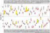 |
Fig. 1 Comparison between spectral-type-based mass estimates (black) and photometric mass estimates (red). Stars where the two estimates are not compatible are highlighted with yellow boxes. |
2.3 Sample selected for this study
The membership analysis mentioned in Sect. 2.2 allowed us to determine that several stars from our initial sample (HIP 52742, HIP 54767, HIP 60855, HIP 65021, HIP 76126, and HIP 81474) have a low chance of being members of the Sco-Cen association. Of these, HIP 52742 and HIP 65021 are part of the 42-strong intermediary sample that we study here. Although they are still relatively young B stars, we decided to remove them from our study, so that our sample is built only from Sco-Cen members, sharing the same environmental conditions associated with this relatively dense young star-forming region.
Another selection bias comes from binarity, since the BEAST survey has been built with the explicit selection of B stars from Sco-Cen with no stellar binary companions between 0.1″ and 6″. However, the BEAST observations themselves have uncovered some of the original sample stars as such intermediate separation stellar binaries. These objects bias the sample because their stellar companions are expected to have a strong impact on planet formation and orbital stability in the separation ranges probed by our data. To be able to derive the unbiased frequency of B stars with no stellar companions within 0.1″−6″ that host at least one planetary-mass companion, we therefore needed to remove any BEAST stars with such an intermediate separation stellar companion from our statistical sample or, if the bias is small enough, try to correct it.
Our BEAST high-contrast imaging data have revealed that eight stars within our initial sample were previously unknown binary stars with a stellar companion within 0.1″−6″, and they are thus outside of the specification of our initial sample. These stars are identified in Table 1 and were found by Gratton et al. (2023), and confirmed bound by our analysis of BEAST data. Among them HIP 52742 has already been rejected because it is not a Sco-Cen member. Six out of the remaining seven have bound stellar companions at a relatively large separation, with a projected semi-major axis (hereafter sma) ranging from 0.26″ to 4.16″ that would strongly bias our sample because they would make a planetary orbit unstable in a large part of the parameter range we probed. According to Holman & Wiegert (1999), for a moderate eccentricity of the binary system, exoplanets cannot have stable orbits if their sma is not at least ~3 times larger than the sma of the stellar companion, and this dynamical instability arises rapidly, within 10000 stellar companion orbits. We therefore also removed these six stars (HIP 50847, HIP 59173, HIP 62434 HIP 63005, HIP 63945, and HIP 74100) from our initial sample.
One last system, HIP 60009 is a tight stellar binary, with a projected sma of 0.146″. We decided to keep it in our final sample because the bias it causes on our sample selection is moderate, and we tried to minimize it as follows. We used the Holman & Wiegert (1999) stability criterion, and for a separation smaller than three times the binary sma, we manually set the completeness of these observations to zero for any companion mass to account for the fact that these two observations could never detect any exoplanet companions in this range where their orbit would be quickly unstable. This is equivalent to removing them from our sample only within the separation range from which we know putative exoplanet companions cannot have stable orbits. We acknowledge that projected separations do not directly translate to sma and that the Holman & Wiegert (1999) stability criterion value of three times the sma is an approximation. However, since the final exoplanet frequency is negligibly affected by varying its value by plus or minus 50% (the effect on the median of the posterior of exoplanet frequency is at the 0.1% level, which is much smaller than our formal error bars), we are confident this bias correction is acceptable.
The 34 stars that we kept in the sample and use in the following statistical study are shown in Table 2, together with their revised properties. Even if we did not use the stars we excluded from the sample in the statistical analysis, we did look for bound substellar companions around all of them. We found none and we make available on Zenodo the detection limits we achieved around these stars, along with the detection limits achieved around the stars we kept in the statistical sample. The median age of this statistical sample is 16.5 Myr, while the median mass of the primary stellar hosts is 4.8 M⊙.
Intermediate separation binaries in sample.
3 Observations and data processing
3.1 Observation setup
All of the observations were taken using SPHERE (Beuzit et al. 2019) in pupil stabilized mode. This mode introduces a field of view (FoV) rotation during the sequence, allowing the use of angular and spectral differential imaging (ASDI, Marois et al. 2006) based post-processing techniques. Each observation uses the infrared dual-band imager and spectrograph (IRDIS, Dohlen et al. 2008) with the N-ALC-YJH-S coronagraph to observe in the K1/K2 bands (except dedicated follow-up observations) in combination with the YJH bands for the integral field spectrograph (IFS, Claudi et al. 2008).
Each observation followed the same observational sequence: first, an unsaturated, non-coronagraphic image – point spread function (PSF) – of the primary was obtained for flux calibration purposes. Second, a coronagraphic exposure with a waffle pattern was applied to the deformable mirror (Cantalloube et al. 2019), for centering purposes. Then, the main coronagraphic exposures were recorded. Finally, another coronagraphic exposure with a waffle pattern was taken, followed by another PSF.
All of the observations were taken in service mode, ensuring the fulfillment of a set of atmospheric conditions for an observation to be accepted. All observations were scheduled to be taken within one hour of meridian crossing, ensuring at least around 20° of parallactic rotation during the coronagraphic sequence. Seeing was also required to be smaller than 0.9″ and the coherence time greater than 4 ms (for more details, see J21). The effective observing conditions as well as the achieved Strehl ratio and raw contrast for the whole survey are shown on Fig. 2. The observing conditions for each individual observation are summarized in figures and tables available on Zenodo.
Sample of stars used for this study’s statistical analysis.
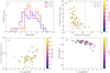 |
Fig. 2 Sample properties and observing conditions. (a) Histogram of the star magnitudes (G, H, and K) for the sample considered in this study. (b) Scatter plot showing the coherence time (τ0) against the seeing with the Strehl ratio color-coded. Data points without Strehl information are colored in white. The boxes delimit the ESO observing categories. (c) Scatter plot showing the 1 sigma raw contrast measured at a separation of 0.5″ (directly measured on the coronographic frame, before post-processing) with respect to the K-band star apparent magnitude. (d) Scatter plot displaying the Strehl ratio as a function of the star apparent magnitude in the G band. |
3.2 Data processing
The whole data reduction was performed on the COBREX Data Center, a modified and improved server based on the High Contrast Data Center, (HC-DC, formerly SPHERE Data Center; Delorme et al. 2017). The COBREX Data Center aims to improve the detection capabilities with existing SPHERE archival data by means of the patch covariance (PACO; Flasseur et al. 2018) algorithm. More specifically, we used PACO ASDI (Flasseur et al. 2020b; Flasseur et al. 2020a) as our primary post-processing algorithm for both IRDIS and IFS, where the initial reduction used the No-ADI (a simple temporal stack), cADI (Marois et al. 2006), and TLOCI-ADI (Marois et al. 2014) algorithms embedded in the SPECAL software (Galicher et al. 2018) in the HC-DC for IRDIS. For IFS, the first reduction also used three algorithms: cADI, TLOCI, and PCA (Soummer et al. 2012).
The prereduction pipeline (i.e., going from raw data to a calibrated 4D datacube) is identical to the one implemented in HC-DC, performing dark, flat, distortion, and bad pixel corrections. The full details on the improvements of the prereduction pipeline as well as the optimization regarding the ASDI mode of PACO, and the obtained performances are described in Chomez et al. (2023a).
The algorithm used in this work, PACO, models the noise using a multi-Gaussian model at a local scale on small patches, allowing for a better estimation of the spatial and spectral correlations of the noise. This modeling improves the contrast achieved between one and two magnitudes at all separations compared to more classical ADI approaches such as TLOCI and PCA. PACO is also a data-driven algorithm, meaning that it requires no hyper-parameters tuning by its user. One of the other key advantages of PACO is its detection map, which is directly interpretable in terms of the signal-to-noise ratio (S/N) of detection. It thus follows the standard normal distribution 𝒩(0, 1) by design, even when the SNR is evaluated close to the target stars where noise is dominated by speckle residual noise. It allows two important features: the first one is a reliable automated detection threshold (fixed for this analysis at the classical 5σ threshold), which is particularly suitable for automated reductions of dozens of datasets. The second one is its statistical guarantee over a detection (i.e., the probability of it being a statistical false positive), which is reliably linked to its S/N.
Using PACO for both instruments allows any systematics related to the use of different algorithms to be removed and the performances of both instruments to be easily compared to each other. Thanks also to the statistically grounded nature of the contrast limits provided by PACO, it allows for the derivation of more reliable constraints on the actual detection limits of the survey and the deeper sensitivity of PACO also enables us to look for new sources undetected by the previous analysis.
4 Detected companions within the sample
The astrometry (separation and PA relative to the host star) and the photometry (IRDIS fluxes and IFS spectrum) of all sources detected within this analysis are made available via a VizieR catalog linked to this article.
4.1 Substellar companions
Two substellar companions have been discovered within BEAST, b Centaurib, by Janson et al. (2021a), and μ2 Sco B by Squicciarini et al. (2022). b Centauri b has a mass of 11 ± 2 MJup, and a mass ratio of 0.1–0.17% with respect to its massive (6–10 M⊙) binary host star system, which is quite close to that of Jupiter in the Solar System. However, its very large projected separation of 560 au and the very high mass of its stellar hosts make it a very distinct type of exoplanet. μ2 Sco B shares many of the peculiar properties of b Centauri b, with a very large separation of 290 au from its very massive (~9M⊙) host and a mass ratio below 0.2%, and if a formation scenario could explain the existence of one of these companions it would certainly be compatible with the other. However, their masses are slightly different, with μ2 Sco B being 14±1 MJup and thus probably straddling the deuterium burning mass, that is to say being used (Lecavelier des Etangs & Lissauer 2022) to draw a border between objects below that 13 MJup limit that are called exoplanets and those above that are called brown dwarfs. In the peculiar case of this study, this definition does not appear to bear any significant physical meaning and would only draw an artificial border between two objects that most likely share a very similar nature.
In the subsequent statistical analysis, we therefore decided to use three different mass cuts: (1) “exoplanets”, for masses below the 13 MJup limits, one detection (b Centauri b); (2) “Exoplanets and Low-mass Brown Dwarfs” (ELBDs), for masses below 30 MJup limits, two detections (b Centauri b and μ2 Sco B); and (3) “substellar objects”, for masses below 73.3 MJup (hydrogen burning minimum mass as defined by Chabrier et al. 2000, at solar metallicity), two detections (b Centaurib and μ2 Sco B). These mass cuts both affect the number of detections in each category but also the completeness of the survey when evaluating the significance of our non-detections.
The choice for the intermediate mass limit of 30 MJup is of course somewhat arbitrary, but motivated by the following argument. The most massive stars systematically surveyed for the presence of giant planets at inner orbits are probably G and K giant stars, with stellar masses typically in the range between 1 and 3 solar masses (see e.g., Wolthoff et al. 2022). In these surveys, the most massive companions range from a few Jupiter masses up to about 25 Jupiter masses continuously, with no obvious gap at certain masses. However, beyond 25 Jupiter masses, very few objects are found, if any4. The next most massive companion after the 30 Jupiter mass limit has a minimum mass of 37 Jupiter masses, but there are indications from Gaia astrometry that its real mass is in excess of 60 Jupiter masses when accounting for inclination. Thus, we opted for a mass limit of 30 Jupiter masses for the ELBDs.
It is to be noted that other companions have been detected or suspected within the overall BEAST sample. First, Squicciarini et al. (2022) identified a promising candidate companion μ2 Sco C, close to the coronographic mask that – if bound – would have a mass of 18±2 MJup. Since our statistical study considers the fraction of systems with at least one companion within a given mass range, it is not affected by the possible existence of another planetary-mass companion in the μ2 Sco system. However, if confirmed, μ2 Sco C, with is relatively short separation of ~20 au, might bring constraints on the formation mechanisms that are quite distinct from the much more distant b Centauri b and μ2 Sco B. Second, Viswanath et al. (2023) discovered a massive ~67 MJup brown dwarf (HIP 81208B) and a very low-mass star (HIP 81208C) orbiting around HIP 81208, and Chomez et al. (2023b) discovered a ~15 MJup planetary-mass companion around the low-mass stellar companion HIP 81208C. Though forming a fascinating hierarchical quadruple system with a chain of relative mass ratios that are difficult to explain by any planet or binary star formation model, the late first epoch observation of HIP 81208 within the BEAST sample puts it outside of the BEAST intermediary sample that is considered by this article (see Sect. 2).
4.2 Identified background sources
With Sco-Cen being located relatively close to the galactic center, it is an area of high stellar density and the large IRDIS FoV consequently yields many detections. Those detections are in vast majority field K and M stars (Parravano et al. 2011), which is consistent with their position on the color magnitude diagram (CMD; see Fig. 3) and they are located much farther away than our target stars. The most effective method to identify those background stars (or, the other way around, find bound companions) is called the common proper motion test. Using (at least) two observations separated by a long enough time baseline, it assesses if the measured motion of a given source between the two observations is consistent with a bound object sharing, in that case, the proper motion of the host star, or a background star with a different (and usually very small) proper motion. This method however has one major flaw: it requires the detection of the sources at both epochs, which can be challenging for faint sources. However, BEAST is conducted in service mode, ensuring consistent performances between all epochs and allowing us to systematically use this technique.
4.3 Identification summary
The sources are classified following three categories (visible in the CMD in Fig. 3): “CC” for confirm companion (i.e., planets, brown dwarfs, and stellar companion), “BCKG_PM” for background sources identified via the proper motion test (see Sect. 4.2), and “BCKG_CMD” for sources detected at one epoch (single epoch stars or unable to re-detect them at a second epoch) that are likely background sources given their positions on the CMD far from the exoplanet parameter range.
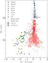 |
Fig. 3 K1-K2 color-magnitude diagram of candidate companions found around the original, 42-strong, sample. Detected sources are represented by the hollow dots while the plain symbols represent the theoretical MLT track (Bonnefoy et al. 2018, Appendix C). |
5 Detection limits
5.1 Dealing with single-epoch stars
Most of the stars present in this sample have been observed at least twice, allowing us to robustly determine the nature of all detected sources via proper motion. However, some stars, as of writing this paper, have only been observed once. If no source has been detected, the detection limits of this single epoch dataset can be used in the following statistical analysis without introducing any bias. However, if a point source is detected, we cannot confirm its nature (bound or background) via proper motion, making the statistical interpretation of the data more challenging. One can use a CMD to try to distinguish between a background source and a bound one but, as shown in Fig. 3, the CMD based on the K1-K2 color is not always discriminant, notably when the exoplanets and background stars track overlap.
In our sample, only one star has such a detection with no proper motion confirmation – HIP 76633 – and we present here how we dealt with this peculiar case in our statistical analysis. The previously undetected and very faint signal unveiled by PACO with a S/N = 5 is located at around 3 as from HIP 76633 and its nature is ambiguous. We modified the detection limits for this peculiar dataset so that we kept the same physical interpretation as detection limits for the single epoch dataset with no companion detected: this allowed to rule out the existence of any companion brighter than this limit in contrast. We therefore wanted the detection limits C at separation s to be expressed in a contrast unit and the contrast Camb of the ambiguous source to be located at the separation samb to verify the following relation:
![Mathematical equation: $\[\forall s \geq s_{\mathrm{amb}}; C(s)=\max \left(C(s), C_{\mathrm{amb}}\right).\]$](/articles/aa/full_html/2024/12/aa51461-24/aa51461-24-eq36.png) (1)
(1)
This effectively made it impossible to detect any companion brighter than the ambiguous source in our detection map. The contrast achieved over the full sample after applying this correction is shown in Fig. 4.
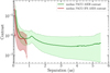 |
Fig. 4 Contrast achieved over the initial, 42-strong sample. The median contrast for both instrument is highlighted with the bold line and the gray area represents the coronographic mask. |
5.2 Achieved contrast and conversion to detection limits expressed in mass
To convert the 2D contrast map into mass maps expressed in MJup, we used a new feature implemented in MADYS (Squicciarini & Bonavita 2022) that allows for this conversion. We used the Gaia DR3 (Gaia Collaboration 2023) parallax and 2 MASS K magnitude for IRDIS and their associated uncertainties provided by Simbad5. To convert magnitude into masses, we used several models – atmo2020 (Phillips et al. 2020), ames-cond (Baraffe et al. 2003), and ames-dusty (Chabrier et al. 2000) – with the resulting variation from model to model being smaller than the mass uncertainties linked to the age uncertainties. In the following we chose to present results obtained with the ames-cond models.
In order to produce probability detection maps for each target and for the sample, we used the EXO-DMC MCMC tool (Bonavita 2020) with a semi-major axis (sma) from 1 to 10000 au and all orbital parameters are uniformly distributed except for the eccentricity, for which a one-sided Gaussian prior was used with 0 mean and 0.3 as sigma (with a max of 1) for the distribution. The average sensitivity using the median age for each star for the whole sample can be seen in Fig. 5, while detection maps using the minimum and maximum ages, the atmo2020 and ames-dusty models, and also the individual detection maps using the ames-cond model for each individual star are available on Zenodo.
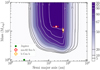 |
Fig. 5 Average detection probability of a companion of given mass/sma in the BEAST intermediary survey using the cond atmospheric model. The two detected planets in this survey are also represented with the mass/sma extracted from Janson et al. (2021a) and Squicciarini et al. (2021). Jupiter is also added to provide a comparison. In the case of b Centauri b, no semi-major axis estimation is available, so we provide its projected separation instead. |
6 The population of the substellar companion around B stars
6.1 Companions around B stars: Jupiter-like mass ratios
Though straddling the planet to brown dwarf definition border, the substellar companions imaged by BEAST have mass ratios relative to their host stars between 0.1 and 0.2%, which is lower than those of other imaged exoplanets and close to the 0.1% of Jupiter relative to the Sun. Since planetary formation takes place in disks around young stars, and since the properties of these protoplanetary disks are heavily related to the stellar mass, the mass ratio is quite informative when investigating the nature and possible formation mechanisms of substellar companions. We therefore converted each detection probability map expressed in Jupiter masses into detection probability maps expressed with the q ratio, that is, the planet to primary star mass ratio, using the nominal masses listed in Table B.1. Once each individual q-ratio map was computed, we interpolated them into a common q-ratio/sma grid and averaged them to produce the final average detection probability map presented in Fig. 6. This figure clearly shows that μ2 Sco B and b Cen b populate a mass-ratio range that is close to that of Jupiter and in the same range as the lowest mass imaged exoplanets, 51 Eri b and AF Lep b. In the case of b Centauri b, the mass ratio can be as low as that of Jupiter if we follow Janson et al. (2021a), and consider the total mass of the central binary (6–10 M⊙) instead of only the primary star (5.9±0.6 M⊙) for the mass-ratio calculation. Though the sma of the BEAST planets are much larger than Jupiter’s, Squicciarini et al. (2022) highlight that the stellar flux at their observed separation is also quite similar to that of Jupiter by the Sun. However, such a continuity in planetary formation from the Sun to a supernova progenitor such as μ2 Sco could come as a surprise. And there are some hints that this similarity might be coincidental: μ2 Sco and b Centauri are among the 20% most massive stars of BEAST, and while we have the detection capability to detect planets with Jupiter-like mass ratios and insulation around lowermass B stars observed by BEAST, we found none, hinting that the population of exoplanets around B stars might differ depending on their mass. However, we know that lower-mass late-B stars can host substellar companions, with HIP 79098AB and HIP 78530 which are two lower-mass B stars outside of BEAST survey that are known to host substellar companions at a large separation (Janson et al. 2019; Lafrenière et al. 2011). Our current sample is too small to be split into higher-than-median-mass and lower-than-median-mass subsamples to provide statistically meaningful constraints on possible variations of giant planet companions’ frequency with B-star mass. The future analysis of the full BEAST sample should provide more informative results on this question.
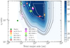 |
Fig. 6 Same as Fig. 5 but expressed in a companion to primary star mass ratio. Several emblematic systems are added to the plot, represented by the hollow diamonds. Data are extracted from Zurlo et al. (2022) for HR 8799 bcde, Desgrange et al. (2022) for HD 95086 b, Blunt et al. (2023) for HIP 65426 b, Lagrange et al. (2020) for β Pictoris b, Brown-Sevilla et al. (2023) for 51 Eri b, and Zhang et al. (2023) for AF Lep b. |
6.2 Frequency of companions around B stars
We wanted to estimate the frequency of planetary systems, so stars with at least one planetary-mass companion. The average survey sensitivity (or completeness) for planetary companions below the IAU maximal mass, and detectable by our data (2–13 MJup) with sma between 10 and 1000 au, is 64.1%. In this range, our sample of 34 stars therefore translates into an effective sample number of 21.8. With one exoplanet found in this range, a first order estimation of the frequency of such companions is 4.6%. However, the second companion, μ2 Sco B, just straddles the 13 MJup limit. If we associate it with the population of ELBDs that we defined in Sect. 4, the average survey sensitivity for such ELBD companions (2–30 MJup) with sma between 10 and 1000 au is 70.5%, resulting in an effective sample number of 24.0. Since we found two ELBDs, a first order estimation of the frequency of such companions is 8.5%.
We thus refined these rough estimates using bayesian probability to be able to derive reliable confidence intervals for the frequency of planetary systems around B stars. We followed the approach described in Carson et al. (2012); Rameau et al. (2013); Lannier et al. (2016) and derived the posterior distributions on the frequency of B-star systems with no stellar companion within 0.1″–6″ that host at least one substellar companion between 10 and 1000 au in various mass ranges.
For a given target j among the N stars within our sample, the mean detection probability of finding a companion of a given mass at a given semi-major axis is pj. We note that pj was derived from the 2D detection limit maps described above. We denote f as the fraction of stars around which there is at least one planet, with a mass included in the interval [2, mmax] MJup (with mmax = 13, 30, 73.3 MJup for exoplanets, ELBDs, and substellar companions, respectively), and for separations inside the interval [10, 1000] au. Then, f pj is the probability of detecting a companion around the star j given its mean detection probability pj and the fraction of stars f hosting at least one companion, and 1 – f pj is the probability of not finding it. The detections and non-detections that are reported for a survey are denoted as dj: dj = 1 for stars around which we found a planet, and 0 otherwise. The likelihood function, L(dj|f), of the data represents the probability that an observation gives dj given the planet fraction f. We have
![Mathematical equation: $\[L\left(d_{j} \mid f\right)=\prod_{j=1}^{N}\left(1-f ~p~_{j}\right)^{1-d_{j}} \times\left(f ~p~_{j}\right)^{d_{j}}.\]$](/articles/aa/full_html/2024/12/aa51461-24/aa51461-24-eq37.png) (2)
(2)
Bayes’ theorem provides the probability density of f, the fraction of stars hosting at least one ELBD given the observed data dj. This probability density is the posterior distribution that represents the distribution of f given the observed data dj:
![Mathematical equation: $\[P(f {\mid} d_{j})=\frac{L(d_{j} {\mid} f) P(f)}{\int_{0}^{1} L(d_{j} {\mid} f) P(f) d f}.\]$](/articles/aa/full_html/2024/12/aa51461-24/aa51461-24-eq38.png) (3)
(3)
In the former equation, P(f) is called the prior distribution. This prior is a distribution reporting any preexisting belief concerning the distribution of f, and it can strongly impact the posterior result when scant observational evidence is available. To minimize the impact of the prior choice, we therefore chose a range in sma and companion masses where our survey sensitivity is good. For the sake of comparison with previous studies, we used a uniform distribution in planetary frequency space as a prior P(f) = 1. The median of the resulting posteriors, as well as the 68.27% confidence intervals (equivalent to ±1σ) and 95.45% confidence intervals (equivalent to ±2σ) are shown in Table 3.
Derived occurrence rates for companions within various mass ranges around our sample of B stars.
6.3 Comparison with the frequency of companions found around solar-type stars
We used the results from the Vigan et al. (2021) SHINE-F150 survey as a comparison to explore whether the companion population is different around B stars and around Sun-like stars.
To account for the observational biases of the SHINE-F150 survey that attributed very high observational priority to some systems where the presence of planets was already known or suspected, we used the statistical weight from Table 1 of Vigan et al. (2021) to each F150 detection. To each detection, this attributes a weight (≤1) that corresponds to the probability that such a stellar system would have been observed if the survey had been unbiased and if observations had been carried out only on the basis of the survey-defined a priori merit function. Following this approach, we attribute 3.4 detections of stellar systems with at least one exoplanet companion to SHINE F150 (accounting for HIP 65426, β Pictoris, HR 8799, and HD 95086, 51 Eri), 4.96 with at least one ELBD (adding HIP 107412 B, HIP 78530 B, GSC8047-0232 B, and AB Pic B), and 8.56 with at least one substellar companion (adding HIP 64892 B, η Tel B, CD-35 2722 B, and Pz Tel B). We then used the same Bayesian statistical framework described above to derive the posterior distribution on the fraction of systems hosting at least one companion from the SHINE-F150 survey. One difference is that we only had access to the average survey sensitivity and not the individual detection maps for the SHINE-F150 survey, and therefore we set f pj to this average sensitivity in Eq. (2) for every star within this survey.
As can be seen in Fig. 7, there is no statistically significant difference in the occurrence rate of either exoplanet, ELBD, or brown dwarf companions. ELBDs might be more common around B stars, but the significance is below 2σ and this possible trend needs to be confirmed by the study of larger samples. In fact, the main difference in the companion properties observed in the BEAST sample is their very large separation from their host star which is replicated by none of the exoplanets or ELBDs from Vigan et al. (2021). However, the Young Suns Exoplanet Survey (YSES) survey (Bohn et al. 2020), targeting solar-type stars located in Sco-Cen (as BEAST stars), shows that these lower-mass stars also harbor exoplanets and ELBDs at very large separations. It is unclear if the absence of such very large separation companions in the SHINE-F150 is a random effect of small number statistics or if it is caused by some underlying physical processes.
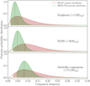 |
Fig. 7 Comparison of the normalized posterior distribution for the frequency of systems with at least one companion below a given mass, between the SHINE-F150 survey targeting mostly solar-type stars and the BEAST survey targeting only B stars. The shaded areas highlight the 95% confidence interval for each distribution and the vertical dashed line highlights the posterior maximum. |
6.4 Comparison to population synthesis models
In order to discuss the formation of observed planets, it is helpful to compare them with synthetic populations that result from population synthesis calculations. Such comparisons, however, are limited, because most population synthesis studies of the disk instability (DI) scenario still lack some physical processes and are typically focused on the planetary population around solar-type stars.
A recent development in population synthesis models in the DI model is the disk instability population synthesis project DIPSY (Schib et al. 2021, 2023, 2024 and in prep.). The authors performed population synthesis of objects that formed through disk fragmentation, including the formation of the star-and-disk system by infall from the molecular cloud core. They studied parameter space in the final stellar mass from 0.05 to 5 M⊙ and find that about 10% of the systems in the stellar mass range above 2.1 M⊙ have at least one surviving companion. Among these systems, results show that a bit less than half would have been excluded from the BEAST survey because they have a stellar mass companion at intermediate separations (see Sect. 2). Based on preliminary results, the fraction of systems with surviving companions that would have been selected is ~6%. This number is in rather good agreement with the companion frequencies given above. Many of these companions also have semi-major axes of hundreds of astronomical units.
However, the companions in systems compatible with the BEAST host star sample have masses from 1.5 MJup to 320 MJup, and most of them are intermediate- or high-mass brown dwarfs: 61% have masses between 30 MJup and 73.3 MJup. The rest are divided into ELBDs (34%) and low-mass stars (5%). Among the systems that do have an ELBD, 64% contain an additional companion more massive than 30 MJup. Only 15% of the ELBDs (corresponding to 5% of the overall companion population) have no other companion in the system, so the probability of finding two such systems and no other substellar companion as observed within the BEAST survey would be very small according to these statistics from DIPSY. It would be even more unlikely if one were to consider the exoplanet subset instead (about one-third of the ELBDs).
At the moment it seems that the companions detected by BEAST are not the most typical outcomes of the DI model. However, it is possible that DIPSY over-estimates the final masses. This could be a result of various reasons such as: an overestimation of gas accretion rate, the assumption of perfect merging due to collisions and ideal merging, and the lack of magnetic fields in the models. Also, we note that DIPSY only studied a stellar mass range up to 5 M⊙ and it is still unclear to what degree the conclusions are applicable to even more massive stars.
The same conclusions can be reached for studies of disk fragmentation around solar-type stars, such as the study by Forgan et al. (2018). These authors performed population synthesis of disk fragmentation, including tidal downsizing and gravitational interaction between fragments. They ignored gas accretion but used a higher initial fragment mass than Schib et al. Their resulting population is again dominated by objects with masses around 80 MJup.
However, recent simulations using state-of-the-art gridbased as well as particle-based 3D magneto-hydrodynamic simulations with self-gravity have uncovered a new regime for disk fragmentation, in which a small seed magnetic field is grown naturally by tapping the energy of the gravitational field (e.g., Riols & Latter 2019; Deng et al. 2020). This results in a dynamo mechanism that is more powerful than magnetorotational instability which rapidly leads to a dynamical important field. In the latter regime, known as “GI dynamo”, disk fragmentation has different characteristics, where the forming clumps are over an order of magnitude smaller in mass relative to conventional DI. In addition, in this case gas accretion is significantly less efficient due to the effect of magnetic pressure (Deng et al. 2021; Kubli et al. 2023). So far, this new fragmentation regime has only been explored for solar-type stars, where the characteristic masses were found to be in the regime of super-Earth and mini-Neptunes. If the mass ratio between stars and clumps is constant in this scenario, one would expect that the inferred distribution of planetary masses in the case of B stars peaks at about one Jupiter mass, so in this case lower masses than the observed 13–15 MJup BEAST companions. Even if this simple scaling does not quantitatively match the observed masses of the companions, it goes qualitatively in the right direction, by lowering the mass of the companions that formed through disk fragmentation. This provides a strong incentive to investigate GI dynamo in the intrinsically more massive disks expected around B stars in future research.
In core accretion, massive companions cannot form at a large separation in situ due to the long core growth timescale (Pollack et al. 1996). The accretion of pebbles may alleviate this problem (Ormel & Klahr 2010), since pebbles can be accreted more efficiently due to the stronger gas drag. However, when both accretion of planetesimals and pebbles are considered, the runaway gas accretion may still be delayed by the late accretion of planetesimals (Kessler & Alibert 2023).
It is, however, possible for massive objects to form closer to the star and be scattered to a large separation later. This scenario should lead to the formation of wide companions only in a minority of systems. For example, the NG76 (100 embryos) population from the New Generation Planetary Population Synthesis (Emsenhuber et al. 2021) features two companions above 1 MJup outside of 100 au in 1000 systems, the 50 embryo population NG75 only has one. However, these populations were conducted for 1 M⊙ stars. A variant population with the same parameters as NG75, except with a stellar mass of 1.5 M⊙, exhibits five wide massive companions. This hints at a larger fraction of such objects around more massive stars. However, the trend of more giants with increasing stellar mass is unlikely to continue to such massive hosts. Instead, the lifetimes of disks around stars more massive than ~3 M⊙ are expected to decline steeply with host mass because the internal photo-evaporation rate has a strong dependence on the stellar mass (Gorti & Hollenbach 2009; Komaki et al. 2021). Lifetimes well below 1 Myr will be too short for core accretion to form giant planets.
6.5 Gravitational capture scenario
The serious challenges for giant planet formation around B stars led Parker & Daffern-Powell (2022, hereafter PD22) to claim that the BEAST ELBDs were so unlikely to have been formed around their current massive hosts that it was more likely they formed around less massive stars (or even as isolated objects) and were later gravitationally captured. In order to investigate this hypothesis, they set up Nsim = 20 simulations where a circle of radius ℓ = 1 pc was filled with 1000 stars following a box-fractal spatial distribution that mimics the initial state of newborn associations (see Daffern-Powell et al. 2022). Given the random sampling of the stellar initial mass function, the number of B-type stars in the cubes, NB, varies between 44 and 65. One half of non-B stars (M* < 2.4 M⊙) are provided with a 1 MJup planet in a circular orbit at a = 30 au. N-body integration allows the dynamical evolution of each simulation to be followed for 10 million years.
A total of 18 planets are captured in the simulations; the frequency of captured planets per star is therefore fp ~ 18/(NB · Nsim) ≈ 0.016, where we assumed a constant NB = 55 for simplicity. Therefore, the probability pcapt of finding at least two captured planets in the 37-star sample considered in this work can be estimated via a binomial distribution,
![Mathematical equation: $\[p_{\text {capt }}=1-\sum_{k=0}^{1}\binom{n}{k} f_{p}^{k}\left(1-f_{p}\right)^{n-k} \approx 0.128,\]$](/articles/aa/full_html/2024/12/aa51461-24/aa51461-24-eq39.png) (4)
(4)
where ![Mathematical equation: $\[\binom{n}{k}=n!/[k!(n-k!)]\]$](/articles/aa/full_html/2024/12/aa51461-24/aa51461-24-eq40.png) is the binomial factor and n = 37. Though this probability is relatively small, it is probably overestimated. The median stellar density, which is a crucial feature of these simulations, is indeed on the order of ~104 pc−3, a value that, in contrast with observations, should result in the presence of dense and gravitationally bound clusters at the age of Sco-Cen (Gieles 2010). This value does not represent the mean density within the simulated volume (n ~ 240 pc−3), but rather the local density of the fractal regions. However, we argue that such a high value of n is not adequate to describe Sco-Cen, which has never been in such a compact configuration in the past (Galli et al. 2018). In addition to this, the assumed frequency of Jupiter-sized planets in wide orbits (fc = 0.5) is unrealistically high if compared to observational evidence (Bowler 2016; Nielsen et al. 2019; Vigan et al. 2021). Therefore, we expect the value of pcaptto be significantly lower.
is the binomial factor and n = 37. Though this probability is relatively small, it is probably overestimated. The median stellar density, which is a crucial feature of these simulations, is indeed on the order of ~104 pc−3, a value that, in contrast with observations, should result in the presence of dense and gravitationally bound clusters at the age of Sco-Cen (Gieles 2010). This value does not represent the mean density within the simulated volume (n ~ 240 pc−3), but rather the local density of the fractal regions. However, we argue that such a high value of n is not adequate to describe Sco-Cen, which has never been in such a compact configuration in the past (Galli et al. 2018). In addition to this, the assumed frequency of Jupiter-sized planets in wide orbits (fc = 0.5) is unrealistically high if compared to observational evidence (Bowler 2016; Nielsen et al. 2019; Vigan et al. 2021). Therefore, we expect the value of pcaptto be significantly lower.
We alternatively tried to quantify an upper limit of the frequency of gravitational capture only based on empirical data. We assessed it by summing the probability of two distinct scenarios: (1) the capture of a Sco-Cen object, either previously bound to a star or flee-floating; and (2) as above, but with the object belonging to the population of old interlopers that happen to share the same physical volume with the association.
The timescale for a close encounter between two stars in a given stellar environment can be estimated as
![Mathematical equation: $\[\tau_{\text {enc }} \approx 3.3 \times 10^{7} ~\mathrm{yr}\left(\frac{100 ~\mathrm{pc}^{-3}}{n}\right)\left(\frac{v_{\infty}}{1 \mathrm{~km} \mathrm{~s}^{-1}}\right)\left(\frac{10^{3} ~\mathrm{au}}{r_{\text {min }}}\right)\left(\frac{M_{\odot}}{m_{t}}\right),\]$](/articles/aa/full_html/2024/12/aa51461-24/aa51461-24-eq41.png) (5)
(5)
where n is the stellar density, v∞ the stellar mean relative speed at infinity, rminthe encounter distance, and mt the total mass participating in the close encounter (Malmberg et al. 2007). The last factor (M⊙/mt) accounts for gravitational focusing – that is, the deflection of stellar trajectories caused by their mutual attraction –, a process that largely extends the effective stellar cross section.
We adopted the stellar density of the relatively compact Lower Scorpius (Squicciarini et al. 2022) group (n ≈ 1 pc−3) as an estimate for a the initial state of a typical star-forming subgroup within Sco-Cen; assuming the present-day velocity dispersion of the Upper Scorpius subgroup (v = 3.0 km s−1, Squicciarini et al. 2021), a typical ml = 5M⊙, and rmin = 1000 au, Eq. (5) yields the following:
![Mathematical equation: $\[\tau_{\text {enc, SC }} \approx 1980 ~{\text{Myr}}.\]$](/articles/aa/full_html/2024/12/aa51461-24/aa51461-24-eq42.png) (6)
(6)
An estimate for the frequency of substellar objects can be obtained based on the results from the SHINE survey (Vigan et al. 2021): the fraction of 1–75 MJup companions with a semi-major axis ∈ [5, 300] au was found to be ![Mathematical equation: $\[5.8_{2.8}^{+4.7}\]$](/articles/aa/full_html/2024/12/aa51461-24/aa51461-24-eq43.png) % and
% and ![Mathematical equation: $\[12.6_{7.1}^{+12.9}\]$](/articles/aa/full_html/2024/12/aa51461-24/aa51461-24-eq44.png) % around FGK and M hosts, respectively. We assumed a constant fraction fc = 10%6. With regard to free-floating objects (5MJup ≲ M ≲ 75 MJup), we estimated their fraction with respect to the total Sco-Cen population as ff ~ 20% (Miret-Roig et al. 2022). In order to set an upper limit on the likelihood of this scenario, we set the efficiency ηcapt of the capture process, that is, the probability that a close encounter with a planet-bearing star or a free-floating object results in a capture event to 100%. Then the expected number of captured objects per close encounter Np,SC after 20 Myr could be computed as
% around FGK and M hosts, respectively. We assumed a constant fraction fc = 10%6. With regard to free-floating objects (5MJup ≲ M ≲ 75 MJup), we estimated their fraction with respect to the total Sco-Cen population as ff ~ 20% (Miret-Roig et al. 2022). In order to set an upper limit on the likelihood of this scenario, we set the efficiency ηcapt of the capture process, that is, the probability that a close encounter with a planet-bearing star or a free-floating object results in a capture event to 100%. Then the expected number of captured objects per close encounter Np,SC after 20 Myr could be computed as
![Mathematical equation: $\[N_{p, \mathrm{SC}} \approx \frac{20 ~\mathrm{Myr}}{460 ~\mathrm{Myr}} \cdot\left(f_{c} \cdot\left(1-f_{\mathrm{f}}\right)+f_{\mathrm{f}}\right)=0.0028.\]$](/articles/aa/full_html/2024/12/aa51461-24/aa51461-24-eq45.png) (7)
(7)
As Np,SC ≪ 1, we assumed the capture probability for a single star to be fp,SC = Np,SC. Considering the whole survey,
![Mathematical equation: $\[p_{capt, SC}=1-\sum_{k=0}^{1}\binom{37}{k} f_{p, S C}^{k}\left(1-f_{p, S C}\right)^{37-k} \approx 0.005.\]$](/articles/aa/full_html/2024/12/aa51461-24/aa51461-24-eq46.png) (8)
(8)
In a similar fashion, we estimated the capture probability of a non-Sco-Cen object to be pcapt,f = 3 · 10−5 (Appendix C). The total upper limit on the probability of the capture scenario is therefore pcapt = pcapt,SC + pcapt,f ≈ pcapt,SC = 0.005, corresponding to a confidence level of 2.8σ on the hypothesis that the two substellar companions are not captured. We stress that since the probability of pcapt linearly depends on the capture efficiency, we set pcapt to one to assess an upper limit of the capture scenario. More realistic values of pcapt, accounting for the possibility of ejection or simply that the companion stays within its birth system, would result in even lower capture probabilities. While these numbers are not sufficient to completely rule out the capture scenario, they indicate that this mechanism is unlikely to account for the population of B-star companions unveiled by BEAST.
7 Conclusion
In this paper, we have discussed several plausible scenarios as pathways to form ELBDs around very massive B stars, namely core fragmentation, gravitational instability in a disk, gravitational capture of free-floating or ejected planets, or core accretion. Although all of them might lead to the formation of planetary-mass objects, none of them provide a straightforward explanation for the population of ELBDs we observed around the stars of the BEAST sample. In the case of gravitational instability, companions are usually more massive and ELBDs make up only the tail of the distribution of companions. It is therefore unlikely to observe two ELBDs and any of the higher-mass brown dwarfs that would be more natural outcomes of gravitational instability. However, including the magnetic field in gravitational instability models might improve the agreement with our observations. When a magnetic field is present in the disk and dynamically important, the character of gravitational instability may indeed be significantly altered, leading to lower-mass companions.
The same issue arises for core fragmentation, which typically forms multiple stellar systems and occasionally brown dwarfs and exoplanet systems (e.g., 2M1207B Chauvin et al. 2004), and is complemented by the very unusual mass ratio of the observed ELBDs, which is almost two orders of magnitude lower than the lowest observed in multiple systems (see Gratton et al. 2023). Core accretion is the typical planet formation scenario that is put forward to explain the formation of Solar System planets, and the mass ratio as well as the stellar insulation at the observed orbital separation for the BEAST ELBDs are of the correct order of magnitude. However, the timescale for the formation of giant planets by core accretion are larger than the quite fast timescale of disk photo-evaporation around a star as hot and luminous as BEAST B stars (Gorti & Hollenbach 2009; Komaki et al. 2021). We also investigated gravitational capture as a distinct pathway to account for the presence of ELBDs around the stars BEAST survey sample. Even when favorable values are used for the various parameters involved in this scenario, we find that gravitational capture is unlikely to account for the observed ELBD populations.
It therefore turns out that none of the scenarios we explored readily explain the population of planetary-mass companions around B stars from our sample. The significant uncertainty affecting each of these scenarios prevents us from identifying which ones could be the least unlikely. At the same time, the physical complexity behind each of these processes means that current models and simulations are still limited in their predictive power, and further progress on the theoretical side must be ultimately guided by observations, such as those presented in this work, probing uncharted regions of parameter space for exoplanets and other substellar objects.
Data availability
Data are available on Zenodo: https://zenodo.org/records/13903381.
Table of all candidate companions detected is available at the CDS via anonymous ftp to cdsarc.cds.unistra.fr (130.79.128.5) or via https://cdsarc.cds.unistra.fr/viz-bin/cat/J/A+A/692/A263
Acknowledgements
This project has received funding from the European Research Council (ERC) under the European Union’s Horizon 2020 research and innovation programme (COBREX; grant agreement n° 885593). SPHERE is an instrument designed and built by a consortium consisting of IPAG (Grenoble, France), MPIA (Heidelberg, Germany), LAM (Marseille, France), LESIA (Paris, France), Laboratoire Lagrange (Nice, France), INAF - Osservatorio di Padova (Italy), Observatoire de Genève (Switzerland), ETH Zürich (Switzerland), NOVA (Netherlands), ONERA (France) and ASTRON (Netherlands) in collaboration with ESO. SPHERE was funded by ESO, with additional contributions from CNRS (France), MPIA (Germany), INAF (Italy), FINES (Switzerland) and NOVA (Netherlands). SPHERE also received funding from the European Commission Sixth and Seventh Framework Programmes as part of the Optical Infrared Coordination Network for Astronomy (OPTICON) under grant number RII3-Ct-2004-001566 for FP6 (2004-2008), grant number 226604 for FP7 (2009-2012) and grant number 312430 for FP7 (2013-2016). This work has made use of the High Contrast Data Centre, jointly operated by OSUG/IPAG (Grenoble), PYTHEAS/LAM/CeSAM (Marseille), OCA/Lagrange (Nice), Observatoire de Paris/LESIA (Paris), and Observatoire de Lyon/CRAL, and is supported by a grant from Labex OSUG@2020 (Investissements d’avenir - ANR10 LABX56). Th.H. and G.-D.M. acknowledge support from the European Research Council under the Horizon 2020 Framework Program via the ERC Advanced Grant Origins 8324 28. G.-D.M. also acknowledges the support of the DFG priority program SPP 1992 “Exploring the Diversity of Extrasolar Planets” under grant MA 9185/1-1. R.G. and S.D. acknowledge the support of PRIN-INAF 2019 Planetary Systems At Early Ages (PLATEA). O.S. acknowledges support from the Swiss National Science Foundation under grant 200021_204847 “PlanetsInTime”. This research has made use of the SIMBAD database and VizieR catalogue access tool, operated at CDS, Strasbourg, France. This work is supported by the French National Research Agency in the framework of the Investissements d’Avenir program (ANR-15-IDEX-02), through the funding of the “Origin of Life” project of the Univ. Grenoble-Alpes. This work was supported by the Action Spécifique Haute Résolution Angulaire (ASHRA) of CNRS/INSU co-funded by CNES. This research has made use of data obtained from or tools provided by the portal exoplanet.eu of The Extrasolar Planets Encyclopaedia.
Appendix A Uncertainties on stellar mass estimates
As described in Sect. 2.2, we derived stellar masses using PARSEC isochrones, so as to be consistent with the underlying age analysis. The typical random uncertainty σr of these, arising from the propagation of the uncertainties on parallax, apparent photometry and age, is on the order of 0.01 < σr ≲ 0.1 M⊙.
However, in addition to unresolved multiplicity and random uncertainties, additional factors can bias the photometric estimate of stellar mass for BEAST stars: 1) the choice of the input evolutionary model, and 2) stellar rotation, which can induce non-negligible luminosity variations in the B-star mass range.
In order to explore the dependency on these factors, we recomputed all stellar masses employing: 1) two different models – MIST (Dotter 2016; Choi et al. 2016) and Geneva (Haemmerlé et al. 2019); 2) PARSEC models with different values of stellar rotation (Nguyen et al. 2022).
A comparison of the results of these various models with the nominal values from the PARSEC nonrotating analysis that we use in this article is shown in Fig. A.1.
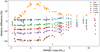 |
Fig. A.1 Systematic difference related to model selection and stellar rotation. Rotation velocities in the legend are expressed in units of the break-up velocity vbreak. |
In order to correctly interpret the results of this comparison, a couple of considerations have to be accounted for. Firstly, if one compares isochronal masses and spectral-type-based masses, a much lower compatibility is observed when using Geneva models, especially in the [4-6] M⊙range: in other words, systematically larger values are obtained using this model. Secondly, we expect the typical rotation velocity of our sample to be << 0.95vbreak. Alecian et al. (2013, hereafter A13) studied the rotation rate of a large sample of young (10 kyr to 10 Myr) Be stars. Even in the worst scenario of nonmagnetic Be stars (see Fig. 5, bottom panel, blue bars of A13), we expect about <5% (15%) of stars to have v sin i > 0.8vbreak for 2.3M⊙ < M < 3.5M⊙ (M > 3.5M⊙). Moreover, only 7 stars of our sample are reported as Be stars by Simbad; standard B stars with no prominent emission lines are expected to possess lower rotation rates. Finally, our stars are generally older than the sample by A13, which shows a clear trend of decreasing angular momentum over time (at least for stars with M>5 M⊙). For all these reasons, we consider it reasonable to (conservatively) assume a minimum fractional uncertainty of 10% on all stellar masses. In the case of μ2 Sco, which is in a mass range where models differ weakly and for which a dedicated analysis, showing evidence for a very low rotation rate, was undertaken in a previous publication (Squicciarini et al. 2022), we retain the nominal PARSEC uncertainty.
A.1 Notes on individual objects
HIP 63210: the classification of this star as B2 (~ 20000 K) is suspicious, as Teffmeasurements from the literature (~ 11000 K) are consistent with a late B. Also, the star is indicated as a SB2 by Chini et al. (2012). An equal-mass B8V binary (with MA = MB ≈ 3.4 M⊙) would be in agreement with the age, temperature and luminosity indicators.
HIP 78384: an equal-mass binary system with MA = MB ≈ 7 M⊙might explain the discrepancy between the two mass estimates; however, the pair separation would have to be < 1 au to be consistent with the non-detection by Rizzuto et al. (2013).
Appendix B Properties of target stars
Revised stellar parameters for all the targets of the BEAST survey. The multiplicity flag mf indicates whether the star is known to be a multiple system (1: Gratton et al. 2023, 2: this work, 3: Chini et al. 2012) or not (0).
Appendix C Assessing the capture scenario for a field object
In order to be properly assessed, a capture scenario cannot neglect the fact that a stellar association, at any point of its history, is nestled in a galactic environment where most of the stars are physically unrelated to the association. Thanks to its peculiar kinematic signature – markedly different from the one of the field –, the association can be said to experience a wind of field stars: we would like to assess here the probability of a BEAST star capturing a substellar object, either isolated or bound to a lower-mass star, from the field.
A list of bona-fide Sco-Cen members was built by considering all the 8878 stars that are listed as members in at least two of the following catalogs: Rizzuto et al. (2015), Galli et al. (2018), Damiani et al. (2019), Luhman & Esplin (2020), Esplin & Luhman (2020), and Luhman (2022). The sample was merged with the 85-star BEAST sample, yielding a sample of Sco-Cen sources, S. Afterwards, we queried the Gaia Archive for all sources located within the box containing S: 152° < α < 268°, −75° < δ < −10°, 4 mas < ϖ < 13 mas. Removing the intersection with S yielded a sample of field stars, F.
For every star in S, we computed the number of stars in F found within 5 pc. We estimate a mean density of nF = 0.34 stars pc−1, four times higher than the corresponding estimate for Sco-Cen sources, nS. We assume nF to be independent of time.
Using Gaia proper motion measurements ![Mathematical equation: $\[\mu_{\alpha}^{*}\]$](/articles/aa/full_html/2024/12/aa51461-24/aa51461-24-eq155.png) and μδ, the 2D mean differential velocity between Sco-Cen stars and field stars can be estimated as
and μδ, the 2D mean differential velocity between Sco-Cen stars and field stars can be estimated as
![Mathematical equation: $\[v_{2 \mathrm{D}}=\sqrt{\left(\left\langle v_{\alpha, s}\right\rangle-\left\langle v_{\alpha, f}\right\rangle\right)^{2}+\left(\left\langle v_{\delta, s}\right\rangle-\left\langle v_{\delta, f}\right\rangle\right)^{2}}=11.2 \mathrm{~km} \mathrm{~s}^{-1},\]$](/articles/aa/full_html/2024/12/aa51461-24/aa51461-24-eq156.png) (C.1)
(C.1)
where vα = 4.74 km s−1 yr · ![Mathematical equation: $\[\mu_{\alpha}^{*}\]$](/articles/aa/full_html/2024/12/aa51461-24/aa51461-24-eq157.png) /ϖ and vδ = 4.74 km s−1 yr · μδ/ϖ and the subscripts s and f indicate stars belonging to S and F, respectively. Assuming the velocity is isotropic, we estimate
/ϖ and vδ = 4.74 km s−1 yr · μδ/ϖ and the subscripts s and f indicate stars belonging to S and F, respectively. Assuming the velocity is isotropic, we estimate ![Mathematical equation: $\[v_{\infty} \approx v_{3 \mathrm{D}}=\sqrt{3 / 2} ~v_{2 \mathrm{D}} \approx 13.7 \mathrm{~km} \mathrm{~s}^{-1}\]$](/articles/aa/full_html/2024/12/aa51461-24/aa51461-24-eq158.png) .
.
According to Eq. 5, a close encounter within 1000 pc with a 5 M⊙ star occurs on a timescale τenc,f = 26.6 Gyr, so that fp,f = 2 · 10−4 (Eq. 7) and finally pcapt = 3 · 10−5 (Eq. 8).
Due to the high relative velocity between field and Sco-Cen stars, the probability of a capture of a field object is negligible compared to the capture of a Sco-Cen object.
References
- Alecian, E., Wade, G. A., Catala, C., et al. 2013, MNRAS, 429, 1027 [Google Scholar]
- Baraffe, I., Chabrier, G., Barman, T. S., Allard, F., & Hauschildt, P. H. 2003, A&A, 402, 701 [NASA ADS] [CrossRef] [EDP Sciences] [Google Scholar]
- Beuzit, J. L., Vigan, A., Mouillet, D., et al. 2019, A&A, 631, A155 [NASA ADS] [CrossRef] [EDP Sciences] [Google Scholar]
- Blunt, S., Balmer, W. O., Wang, J. J., et al. 2023, AJ, 166, 257 [NASA ADS] [CrossRef] [Google Scholar]
- Bohn, A. J., Kenworthy, M. A., Ginski, C., et al. 2020, MNRAS, 492, 431 [Google Scholar]
- Bohn, A. J., Ginski, C., Kenworthy, M. A., et al. 2021, A&A, 648, A73 [NASA ADS] [CrossRef] [EDP Sciences] [Google Scholar]
- Bonavita, M. 2020, Astrophysics Source Code Library [record ascl:2010.008] [Google Scholar]
- Bonnefoy, M., Perraut, K., Lagrange, A. M., et al. 2018, A&A, 618, A63 [NASA ADS] [CrossRef] [EDP Sciences] [Google Scholar]
- Bowler, B. P. 2016, PASP, 128, 102001 [Google Scholar]
- Brown-Sevilla, S. B., Maire, A. L., Mollière, P., et al. 2023, A&A, 673, A98 [NASA ADS] [CrossRef] [EDP Sciences] [Google Scholar]
- Cantalloube, F., Dohlen, K., Milli, J., Brandner, W., & Vigan, A. 2019, The Messenger, 176, 25 [NASA ADS] [Google Scholar]
- Carson, J., Thalmann, C., Janson, M., et al. 2012, AAS Meeting Abstracts, 219, 432.02 [NASA ADS] [Google Scholar]
- Chabrier, G., Baraffe, I., Allard, F., & Hauschildt, P. 2000, ApJ, 542, 464 [Google Scholar]
- Chauvin, G., Lagrange, A. M., Dumas, C., et al. 2004, A&A, 425, L29 [NASA ADS] [CrossRef] [EDP Sciences] [Google Scholar]
- Chini, R., Hoffmeister, V. H., Nasseri, A., Stahl, O., & Zinnecker, H. 2012, MNRAS, 424, 1925 [Google Scholar]
- Choi, J., Dotter, A., Conroy, C., et al. 2016, ApJ, 823, 102 [Google Scholar]
- Chomez, A., Lagrange, A. M., Delorme, P., et al. 2023a, A&A, 675, A205 [NASA ADS] [CrossRef] [EDP Sciences] [Google Scholar]
- Chomez, A., Squicciarini, V., Lagrange, A. M., et al. 2023b, A&A, 676, L10 [NASA ADS] [CrossRef] [EDP Sciences] [Google Scholar]
- Claudi, R. U., Turatto, M., Gratton, R. G., et al. 2008, SPIE Conf. Ser., 7014, 70143E [Google Scholar]
- Cutri, R. M., Skrutskie, M. F., van Dyk, S., et al. 2003, VizieR Online Data Catalog: II/246 [Google Scholar]
- Daffern-Powell, E. C., Parker, R. J., & Quanz, S. P. 2022, MNRAS, 514, 920 [Google Scholar]
- Damiani, F., Prisinzano, L., Pillitteri, I., Micela, G., & Sciortino, S. 2019, A&A, 623, A112 [NASA ADS] [CrossRef] [EDP Sciences] [Google Scholar]
- Delorme, P., Meunier, N., Albert, D., et al. 2017, in SF2A-2017: Proceedings of the Annual meeting of the French Society of Astronomy and Astrophysics, eds. C. Reylé, P. Di Matteo, F. Herpin, et al. [Google Scholar]
- Deng, H., Mayer, L., & Latter, H. 2020, ApJ, 891, 154 [Google Scholar]
- Deng, H., Mayer, L., & Helled, R. 2021, Nat. Astron., 5, 967 [Google Scholar]
- Desgrange, C., Chauvin, G., Christiaens, V., et al. 2022, A&A, 664, A139 [NASA ADS] [CrossRef] [EDP Sciences] [Google Scholar]
- Dohlen, K., Langlois, M., Saisse, M., et al. 2008, SPIE Conf. Ser., 7014, 70143L [Google Scholar]
- Dotter, A. 2016, ApJS, 222, 8 [Google Scholar]
- Emsenhuber, A., Mordasini, C., Burn, R., et al. 2021, A&A, 656, A70 [NASA ADS] [CrossRef] [EDP Sciences] [Google Scholar]
- Esplin, T. L., & Luhman, K. L. 2020, AJ, 159, 282 [Google Scholar]
- Flasseur, O., Denis, L., Thiébaut, É., & Langlois, M. 2018, A&A, 618, A138 [NASA ADS] [CrossRef] [EDP Sciences] [Google Scholar]
- Flasseur, O., Denis, L., Thiébaut, É., & Langlois, M. 2020a, A&A, 637, A9 [NASA ADS] [CrossRef] [EDP Sciences] [Google Scholar]
- Flasseur, O., Denis, L., Thiébaut, É., & Langlois, M. 2020b, A&A, 634, A2 [Google Scholar]
- Forgan, D. H., Hall, C., Meru, F., & Rice, W. K. M. 2018, MNRAS, 474, 5036 [Google Scholar]
- Gagné, J., Mamajek, E. E., Malo, L., et al. 2018, ApJ, 856, 23 [Google Scholar]
- Gaia Collaboration (Brown, A. G. A., et al.) 2018, A&A, 616, A1 [NASA ADS] [CrossRef] [EDP Sciences] [Google Scholar]
- Gaia Collaboration (Vallenari, A., et al.) 2023, A&A, 674, A1 [NASA ADS] [CrossRef] [EDP Sciences] [Google Scholar]
- Galicher, R., Boccaletti, A., Mesa, D., et al. 2018, A&A, 615, A92 [NASA ADS] [CrossRef] [EDP Sciences] [Google Scholar]
- Galli, P. A. B., Joncour, I., & Moraux, E. 2018, MNRAS, 477, L50 [Google Scholar]
- Gieles, M. 2010, IAU Symp., 266, 69 [NASA ADS] [Google Scholar]
- Gillon, M., Jehin, E., Lederer, S. M., et al. 2016, Nature, 533, 221 [Google Scholar]
- Gorti, U., & Hollenbach, D. 2009, ApJ, 690, 1539 [Google Scholar]
- Gratton, R., Squicciarini, V., Nascimbeni, V., et al. 2023, A&A, 678, A93 [NASA ADS] [CrossRef] [EDP Sciences] [Google Scholar]
- Haemmerlé, L., Eggenberger, P., Ekström, S., et al. 2019, A&A, 624, A137 [NASA ADS] [CrossRef] [EDP Sciences] [Google Scholar]
- Holman, M. J., & Wiegert, P. A. 1999, AJ, 117, 621 [Google Scholar]
- Janson, M., Bonavita, M., Klahr, H., et al. 2011, ApJ, 736, 89 [Google Scholar]
- Janson, M., Asensio-Torres, R., André, D., et al. 2019, A&A, 626, A99 [EDP Sciences] [Google Scholar]
- Janson, M., Gratton, R., Rodet, L., et al. 2021a, Nature, 600, 231 [NASA ADS] [CrossRef] [Google Scholar]
- Janson, M., Squicciarini, V., Delorme, P., et al. 2021b, A&A, 646, A164 [NASA ADS] [CrossRef] [EDP Sciences] [Google Scholar]
- Kervella, P., Arenou, F., & Thévenin, F. 2022, A&A, 657, A7 [NASA ADS] [CrossRef] [EDP Sciences] [Google Scholar]
- Kessler, A., & Alibert, Y. 2023, A&A, 674, A144 [NASA ADS] [CrossRef] [EDP Sciences] [Google Scholar]
- Kiefer, F., Lagrange, A.-M., Rubini, P., & Philipot, F. 2024, arXiv e-print [arXiv:2409.16992] [Google Scholar]
- Komaki, A., Nakatani, R., & Yoshida, N. 2021, ApJ, 910, 51 [NASA ADS] [CrossRef] [Google Scholar]
- Kubli, N., Mayer, L., & Deng, H. 2023, MNRAS, 525, 2731 [NASA ADS] [CrossRef] [Google Scholar]
- Lafrenière, D., Jayawardhana, R., Janson, M., et al. 2011, ApJ, 730, 42 [Google Scholar]
- Lagrange, A. M., Rubini, P., Nowak, M., et al. 2020, A&A, 642, A18 [NASA ADS] [CrossRef] [EDP Sciences] [Google Scholar]
- Lannier, J., Delorme, P., Lagrange, A. M., et al. 2016, A&A, 596, A83 [NASA ADS] [CrossRef] [EDP Sciences] [Google Scholar]
- Lecavelier des Etangs, A., & Lissauer, J. J. 2022, New A Rev., 94, 101641 [Google Scholar]
- Leike, R. H., Glatzle, M., & Enßlin, T. A. 2020, A&A, 639, A138 [NASA ADS] [CrossRef] [EDP Sciences] [Google Scholar]
- Luhman, K. L. 2022, AJ, 163, 24 [NASA ADS] [CrossRef] [Google Scholar]
- Luhman, K. L., & Esplin, T. L. 2020, AJ, 160, 44 [Google Scholar]
- Malmberg, D., de Angeli, F., Davies, M. B., et al. 2007, MNRAS, 378, 1207 [NASA ADS] [CrossRef] [Google Scholar]
- Marois, C., Lafrenière, D., Doyon, R., Macintosh, B., & Nadeau, D. 2006, ApJ, 641, 556 [Google Scholar]
- Marois, C., Correia, C., Véran, J.-P., & Currie, T. 2014, IAU Symp., 299, 48 [NASA ADS] [Google Scholar]
- Miret-Roig, N., Bouy, H., Raymond, S. N., et al. 2022, Nat. Astron., 6, 89 [NASA ADS] [CrossRef] [Google Scholar]
- Moe, M., & Di Stefano, R. 2017, ApJS, 230, 15 [Google Scholar]
- Nguyen, C. T., Costa, G., Girardi, L., et al. 2022, A&A, 665, A126 [NASA ADS] [CrossRef] [EDP Sciences] [Google Scholar]
- Nielsen, E. L., De Rosa, R. J., Macintosh, B., et al. 2019, AJ, 158, 13 [Google Scholar]
- Ormel, C., & Klahr, H. 2010, A&A, 520, A43 [NASA ADS] [CrossRef] [EDP Sciences] [Google Scholar]
- Parker, R. J., & Daffern-Powell, E. C. 2022, MNRAS, 516, L91 [Google Scholar]
- Parravano, A., McKee, C. F., & Hollenbach, D. J. 2011, ApJ, 726, 27 [Google Scholar]
- Pecaut, M. J., & Mamajek, E. E. 2013, ApJS, 208, 9 [Google Scholar]
- Pecaut, M. J., & Mamajek, E. E. 2016, MNRAS, 461, 794 [Google Scholar]
- Phillips, M. W., Tremblin, P., Baraffe, I., et al. 2020, A&A, 637, A38 [NASA ADS] [CrossRef] [EDP Sciences] [Google Scholar]
- Pollack, J. B., Hubickyj, O., Bodenheimer, P., et al. 1996, Icarus, 124, 62 [NASA ADS] [CrossRef] [Google Scholar]
- Rameau, J., Chauvin, G., Lagrange, A. M., et al. 2013, A&A, 553, A60 [NASA ADS] [CrossRef] [EDP Sciences] [Google Scholar]
- Reffert, S., Bergmann, C., Quirrenbach, A., Trifonov, T., & Künstler, A. 2015, A&A, 574, A116 [NASA ADS] [CrossRef] [EDP Sciences] [Google Scholar]
- Riols, A., & Latter, H. 2019, MNRAS, 482, 3989 [Google Scholar]
- Rizzuto, A. C., Ireland, M. J., & Robertson, J. G. 2011, MNRAS, 416, 3108 [Google Scholar]
- Rizzuto, A. C., Ireland, M. J., Robertson, J. G., et al. 2013, MNRAS, 436, 1694 [Google Scholar]
- Rizzuto, A. C., Ireland, M. J., & Kraus, A. L. 2015, MNRAS, 448, 2737 [NASA ADS] [CrossRef] [Google Scholar]
- Schib, O., Mordasini, C., Wenger, N., Marleau, G. D., & Helled, R. 2021, A&A, 645, A43 [NASA ADS] [CrossRef] [EDP Sciences] [Google Scholar]
- Schib, O., Mordasini, C., & Helled, R. 2023, A&A, 669, A31 [NASA ADS] [CrossRef] [EDP Sciences] [Google Scholar]
- Schib, O., Mordasini, C., Helled, R., & Emsenhuber, A. 2024, in European Planetary Science Congress, EPSC2024-901 [Google Scholar]
- Soummer, R., Pueyo, L., & Larkin, J. 2012, ApJ, 755, L28 [Google Scholar]
- Squicciarini, V., & Bonavita, M. 2022, A&A, 666, A15 [NASA ADS] [CrossRef] [EDP Sciences] [Google Scholar]
- Squicciarini, V., Gratton, R., Bonavita, M., & Mesa, D. 2021, MNRAS, 507, 1381 [NASA ADS] [CrossRef] [Google Scholar]
- Squicciarini, V., Gratton, R., Janson, M., et al. 2022, A&A, 664, A9 [NASA ADS] [CrossRef] [EDP Sciences] [Google Scholar]
- van Leeuwen, F. 2007, A&A, 474, 653 [CrossRef] [EDP Sciences] [Google Scholar]
- Vigan, A., Fontanive, C., Meyer, M., et al. 2021, A&A, 651, A72 [EDP Sciences] [Google Scholar]
- Viswanath, G., Janson, M., Gratton, R., et al. 2023, A&A, 675, A54 [NASA ADS] [CrossRef] [EDP Sciences] [Google Scholar]
- Wenger, M., Ochsenbein, F., Egret, D., et al. 2000, A&AS, 143, 9 [NASA ADS] [CrossRef] [EDP Sciences] [Google Scholar]
- Wolthoff, V., Reffert, S., Quirrenbach, A., et al. 2022, A&A, 661, A63 [NASA ADS] [CrossRef] [EDP Sciences] [Google Scholar]
- Zhang, Z., Mollière, P., Hawkins, K., et al. 2023, AJ, 166, 198 [NASA ADS] [CrossRef] [Google Scholar]
- Zurlo, A., Goździewski, K., Lazzoni, C., et al. 2022, A&A, 666, A133 [NASA ADS] [CrossRef] [EDP Sciences] [Google Scholar]
In order to remove systematic uncertainties related to the modeling of low-mass stars (see discussion in Squicciarini & Bonavita 2022, and references therein), only stars with M > 0.85 M⊙ were considered.
According to PARSEC isochrones, a ~ 2 M⊙ companion to a 15 Myr, 5 M⊙ star (i.e., a mass ratio q ~ 0.4) is needed to cause a ~ 10% flux offset in the G band – approximately corresponding to 0.1 mag – in the system’s photometry. Multiple systems with a smaller q are well approximated by the single-star model. This typical threshold q value is between 0.4 and 0.6 for the age and mass range of BEAST stars.
Approximately corresponding to a 10% error on Teff.
See e.g., the continuously updated table with planets discovered around giant stars at https://www.lsw.uni-heidelberg.de/users/sreffert/giantplanets/giantplanets.php
The value is a comfortable upper limit since the BEAST survey is virtually insensitive to 1 MJup ≲ M ≲ 2 MJup objects and only weakly sensitive to the regime 2 MJup ≲ M ≲ 3 MJup (Fig. 5).
All Tables
Derived occurrence rates for companions within various mass ranges around our sample of B stars.
Revised stellar parameters for all the targets of the BEAST survey. The multiplicity flag mf indicates whether the star is known to be a multiple system (1: Gratton et al. 2023, 2: this work, 3: Chini et al. 2012) or not (0).
All Figures
|
Fig. 1 Comparison between spectral-type-based mass estimates (black) and photometric mass estimates (red). Stars where the two estimates are not compatible are highlighted with yellow boxes. |
| In the text | |
|
Fig. 2 Sample properties and observing conditions. (a) Histogram of the star magnitudes (G, H, and K) for the sample considered in this study. (b) Scatter plot showing the coherence time (τ0) against the seeing with the Strehl ratio color-coded. Data points without Strehl information are colored in white. The boxes delimit the ESO observing categories. (c) Scatter plot showing the 1 sigma raw contrast measured at a separation of 0.5″ (directly measured on the coronographic frame, before post-processing) with respect to the K-band star apparent magnitude. (d) Scatter plot displaying the Strehl ratio as a function of the star apparent magnitude in the G band. |
| In the text | |
|
Fig. 3 K1-K2 color-magnitude diagram of candidate companions found around the original, 42-strong, sample. Detected sources are represented by the hollow dots while the plain symbols represent the theoretical MLT track (Bonnefoy et al. 2018, Appendix C). |
| In the text | |
|
Fig. 4 Contrast achieved over the initial, 42-strong sample. The median contrast for both instrument is highlighted with the bold line and the gray area represents the coronographic mask. |
| In the text | |
|
Fig. 5 Average detection probability of a companion of given mass/sma in the BEAST intermediary survey using the cond atmospheric model. The two detected planets in this survey are also represented with the mass/sma extracted from Janson et al. (2021a) and Squicciarini et al. (2021). Jupiter is also added to provide a comparison. In the case of b Centauri b, no semi-major axis estimation is available, so we provide its projected separation instead. |
| In the text | |
|
Fig. 6 Same as Fig. 5 but expressed in a companion to primary star mass ratio. Several emblematic systems are added to the plot, represented by the hollow diamonds. Data are extracted from Zurlo et al. (2022) for HR 8799 bcde, Desgrange et al. (2022) for HD 95086 b, Blunt et al. (2023) for HIP 65426 b, Lagrange et al. (2020) for β Pictoris b, Brown-Sevilla et al. (2023) for 51 Eri b, and Zhang et al. (2023) for AF Lep b. |
| In the text | |
|
Fig. 7 Comparison of the normalized posterior distribution for the frequency of systems with at least one companion below a given mass, between the SHINE-F150 survey targeting mostly solar-type stars and the BEAST survey targeting only B stars. The shaded areas highlight the 95% confidence interval for each distribution and the vertical dashed line highlights the posterior maximum. |
| In the text | |
|
Fig. A.1 Systematic difference related to model selection and stellar rotation. Rotation velocities in the legend are expressed in units of the break-up velocity vbreak. |
| In the text | |
Current usage metrics show cumulative count of Article Views (full-text article views including HTML views, PDF and ePub downloads, according to the available data) and Abstracts Views on Vision4Press platform.
Data correspond to usage on the plateform after 2015. The current usage metrics is available 48-96 hours after online publication and is updated daily on week days.
Initial download of the metrics may take a while.