| Issue |
A&A
Volume 692, December 2024
|
|
|---|---|---|
| Article Number | A160 | |
| Number of page(s) | 29 | |
| Section | Interstellar and circumstellar matter | |
| DOI | https://doi.org/10.1051/0004-6361/202451567 | |
| Published online | 12 December 2024 | |
Toward a robust physical and chemical characterization of heterogeneous lines of sight: The case of the Horsehead nebula
1
IRAM,
300 rue de la Piscine,
38406
Saint Martin d’Hères,
France
2
Université de Toulon, Aix Marseille Univ, CNRS, IM2NP,
Toulon,
France
3
LERMA, Observatoire de Paris, PSL Research University, CNRS, Sorbonne Universités,
75014
Paris,
France
4
Instituto de Física Fundamental (CSIC),
Calle Serrano 121,
28006,
Madrid,
Spain
5
National Radio Astronomy Observatory,
520 Edgemont Road,
Charlottesville,
VA
22903,
USA
6
Laboratoire d’Astrophysique de Bordeaux, Univ. Bordeaux, CNRS,
B18N, Allée Geoffroy Saint-Hilaire,
33615
Pessac,
France
7
Univ. Grenoble Alpes, Inria, CNRS, Grenoble INP, GIPSA-Lab,
Grenoble
38000,
France
8
Univ. Lille, CNRS, Centrale Lille,
UMR 9189 – CRIStAL,
59651
Villeneuve d’Ascq,
France
9
LERMA, Observatoire de Paris, PSL Research University, CNRS, Sorbonne Universités,
92190
Meudon,
France
10
Institut de Recherche en Astrophysique et Planétologie (IRAP), Université Paul Sabatier,
Toulouse cedex 4,
France
11
Instituto de Astrofísica, Pontificia Universidad Católica de Chile,
Av. Vicuña Mackenna 4860, 7820436 Macul,
Santiago,
Chile
12
Laboratoire de Physique de l’Ecole normale supérieure, ENS, Université PSL, CNRS, Sorbonne Université, Université de Paris,
Sorbonne Paris Cité,
Paris,
France
13
Jet Propulsion Laboratory, California Institute of Technology,
4800 Oak Grove Drive,
Pasadena,
CA
91109,
USA
14
Department of Earth, Environment, and Physics, Worcester State University,
Worcester,
MA
01602,
USA
15
Harvard-Smithsonian Center for Astrophysics,
60 Garden Street,
Cambridge,
MA,
02138,
USA
16
School of Physics and Astronomy, Cardiff University,
Queen’s buildings,
Cardiff
CF24 3AA,
UK
17
Department of Astronomy, University of Florida,
PO Box 112055,
Gainesville,
FL
32611,
USA
★ Corresponding author; This email address is being protected from spambots. You need JavaScript enabled to view it.
Received:
18
July
2024
Accepted:
23
September
2024
Abstract
Context. Dense and cold molecular cores and filaments are surrounded by an envelope of translucent gas. Some of the low-J emission lines of CO and HCO+ isotopologues are more sensitive to the conditions either in the translucent environment or in the dense and cold one because their intensities result from a complex interplay of radiative transfer and chemical properties of these heterogeneous lines of sight (LoSs).
Aims. We extend our previous single-zone modeling with a more realistic approach that introduces multiple layers to take account of possibly varying conditions along the LoS. We used the IRAM-30m data from the ORION-B large program toward the Horsehead nebula in order to demonstrate our method’s capability and effectiveness.
Methods. We propose a cloud model composed of three homogeneous slabs of gas along each LoS, representing an outer envelope and a more shielded inner layer. We used the non-LTE radiative transfer code RADEX to model the line profiles from the kinetic temperature (Tkin), the volume density (nH2), kinematics, and chemical properties of the different layers. We then used a fast and robust maximum likelihood estimator to simultaneously fit the observed lines of the CO and HCO+ isotopologues. To limit the variance on the estimates, we propose a simple chemical model by constraining the column densities.
Results. A single-layer model cannot reproduce the spectral line asymmetries that result from a combination of different radial velocities and absorption effects among layers. A minimal heterogeneous model (three layers only) is sufficient for the Horsehead application, as it provides good fits of the seven fitted lines over a large part of the studied field of view. The decomposition of the intensity into three layers allowed us to discuss the distribution of the estimated physical or chemical properties along the LoS. About 80% of the 12CO integrated intensity comes from the outer envelope, while ~55% of the integrated intensity of the (1 − 0) and (2 − 1) lines of C18O comes from the inner layer. For the lines of the 13CO and the HCO+ isotopologues, integrated intensities are more equally distributed over the cloud layers. The estimated column density ratio N(13CO)/N(C18O) in the envelope increases with decreasing visual extinction, and it reaches 25 in the pillar outskirts. While the inferred Tkin of the envelope varies from 25 to 40 K, that of the inner layer drops to ~15 K in the western dense core. The estimated nH2 in the inner layer is ~3 × 104 cm−3 toward the filament, and it increases by a factor of ten toward dense cores.
Conclusions. Our proposed method correctly retrieves the physical and chemical properties of the Horsehead nebula. It also offers promising prospects for less supervised model fits of wider-field datasets.
Key words: methods: data analysis / methods: statistical / ISM: abundances / ISM: clouds / ISM: lines and bands / photon-dominated region (PDR)
© The Authors 2024
 Open Access article, published by EDP Sciences, under the terms of the Creative Commons Attribution License (https://creativecommons.org/licenses/by/4.0), which permits unrestricted use, distribution, and reproduction in any medium, provided the original work is properly cited.
This article is published in open access under the Subscribe to Open model. This email address is being protected from spambots. You need JavaScript enabled to view it. to support open access publication.
1 Introduction
Star formation takes place in giant molecular clouds (GMCs) with an overall small efficiency (Shu et al. 1987; Lada & Lada 2003; Kennicutt & Evans 2012; Schinnerer & Leroy 2024, and references therein). Current star formation theory assumes that a bottleneck comes from the formation of dense cores of density ≳ 104 cm−3 (e.g., Bergin & Tafalla 2007), and recent observations suggest that the galactic environment of a GMC impacts its star formation efficiency (Schinnerer & Leroy 2024).
Although GMCs show an internal structure, which can be probed by observing various molecular lines, a typical representation of a GMC is still lacking. This is significant, as it will benchmark the general understanding of the molecular interstellar medium (ISM) in the Milky Way and nearby galaxies. To achieve this representation, realistic large-scale maps of the cloud physical parameters (column densities, volume density, kinetic temperature, and kinematics) are needed for a representative sample of GMCs in the Milky Way. While the current generation of millimeter observatories, such as the IRAM-30m telescope, NOEMA, or ALMA, enables surveys of tens of molecular lines over wide fields of view (e.g., Pety et al. 2017; Kauffmann et al. 2017; Evans et al. 2020; Barnes et al. 2020; Tafalla et al. 2021; Dame & Lada 2023), there is still a lack of fully relevant methods to easily extract the physical and chemical information that these lines encode.
It is thus important to develop fast and rigorous methods to infer 2D maps of cloud physical parameters from modern-day large-scale, well-resolved multi-line maps. In order to accurately fit the observed line intensities and profiles, these methods must take into account that lines of sight (LoSs) contain gas components with different physical conditions and chemical compositions, which often interact radiatively. Previous studies based on coupled non-local thermodynamic equilibrium (non-LTE) radiative transfer and chemical models were designed to fit high angular resolution multi-line observations toward either a single line of sight of interest or narrow fields of view (see, e.g., Goicoechea et al. 2006, 2009, toward the Horsehead PDR). With the ability to conduct large mapping surveys of molecular gas lines at high spatial resolution, the main challenge now is to develop robust methods for much larger areas.
The simplest modeling geometry to do this with is a homogeneous LoS composed of a single component. However, the line emission maps of Pety et al. (2017); Kauffmann et al. (2017); Barnes et al. (2020) suggest that the emission comes from gas with different physical conditions, at least along the LoSs toward filaments and dense cores. Roueff et al. (2024) document inconsistencies in the inferred gas conditions when simultaneously analyzing different molecular lines with a non-LTE radiative transfer cloud model of a homogeneous slab of gas. For instance, simultaneously fitting different sets of lines (such as 12CO, 13CO, and HCO+ on the one hand and C18O and H13CO+ on the other) in the same field of view yields drastic differences in inferred volume densities up to one order of magnitude. This suggests that model misspecifications prevent us from deciphering the information provided by emission lines. In this study, we develop a three-layer model to consider the heterogeneous conditions along the LoSs toward filaments or dense cores while keeping the model as simple as possible. This multi-layer cloud model is based on routinely used radiative transfer methods. In spite of its simplicity, it allows us to analyze the contribution of the different layers to the line emission in addition to delivering an estimation of the physical quantities with their confidence interval.
The region under study is the Horsehead nebula (Barnard 33), located in the Orion B cloud. This region is an ideal candidate for evaluating the model’s performance for several reasons. First, this nebula hosts a diversity of physico-chemical regimes such as photon dissociation regions (PDRs); translucent regions (Tkin > 30 K,  cm−3); and dense cores (Tkin < 15 K,
  cm−3). Corresponding density and temperature gradients (e.g., within the PDR Hernández-Vera et al. (2023)) and steep changes of the gas chemical state detected along the LoS suggest that a standard radiative transfer analysis within a homogeneous cloud model is a too simple description for this region. Second, the Horsehead nebula has been the subject of numerous studies, from the analysis of its kinematics (e.g., Hily-Blant et al. 2005; Gaudel et al. 2023) to the dissection of the chemistry and structure of its PDR (e.g., Gerin et al. 2009; Guzmán et al. 2011, 2012; Pety et al. 2012; Gratier et al. 2013; Guzmán et al. 2013, 2014, 2015; Fuente et al. 2017; Hernández-Vera et al. 2023; Abergel et al. 2024). Applying our model to this familiar, albeit complex object, is therefore an opportunity to better diagnose the relevance of the proposed technique.
The paper is organized as follows. Section 2 briefly describes the observations. The radiative transfer and noise models as well as the fitting method and the estimation of the confidence intervals are described in Sect. 3. The physical and chemical assumptions are justified in Sect. 4. Section 5 presents the results on the intensity decomposition, the gas velocity field, the estimated chemical abundances, and the physical conditions (kinetic temperature and volume density). Section 6 discusses the estimated abundances. Finally, Sect. 7 summarizes our findings.
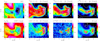 |
Fig. 1 Spatial distribution of the peak main beam temperature (Tmb) of the (1 − 0) line of the CO and HCO+ isotopologues as well as of the dust temperature (Tdust), visual extinction (AV), and the ratio of the far UV field over the visual extinction (G0/AV) toward the Horsehead nebula. The used projection is the Azimuthal one rotated by 14° around the center of coordinates RA= 05h40m54.27s, Dec= −02°28′00.00″ in the International Celestial Reference System. Contours of the dust visual extinction at 3, 7, and 16 magnitudes are overlaid on each panel. The crosses and circles show lines of sight that are studied in more detail in this paper (see Table 2 for the corresponding coordinates). |
2 Observations
In this study, we use the same data as in Roueff et al. (2024). As they are fully described there, we only summarize useful information here. The field of view contains the Horsehead nebula. Figure 1 shows the spatial distribution of various tracers of the interstellar gas and dust. The data include the low-J transitions of the isotopologues of carbon monoxide (12CO, 13CO, and C18O) and formylium (HCO+ and H13CO+), observed with the IRAM-30m telescope, as part of the ORION-B large program (PIs: J. Pety & M. Gerin). Table 1 lists the properties of the studied emission lines.
The data also include maps of the dust visual extinction (AV) and of dust temperature (Tdust) derived by Lombardi et al. (2014) and Pety et al. (2017) from the Herschel Gould Belt Survey data (André et al. 2010). We used the far UV illumination parameter (G0) derived by Santa-Maria et al. (2023) to compute a map of the ratio G0/AV. Assuming that there is some relation between the volume and column densities, G0 /AV is a proxy of the ratio of the far UV field by the volume density, which controls to first order the chemistry of PDRs. In this study, the spatial distribution of AV, Tdust, and G0/AV only serve i) as references to locate the different media that are present in the Horsehead nebula, and ii) to compute the chemical abundances. In particular, they are not taken into account as prior knowledge to characterize the gas physical properties along each LoS.
We identify in Fig. 1 two dense cores where AV > 16 mag and Tdust < 20 K. These cores correspond to the LoSs where the H13CO+ (1 − 0) line is clearly detected. The maximum of the H13CO+ (1 − 0) intensity also corresponds to the maximum of the visual extinction or gas column density. In each core, the C18O (1 − 0) emission peaks are offset compared to the peaks of the H2 column density. This might be due to C18O depletion from the gas phase, as CO is known to freeze on grain mantles when the dust grains are cold enough (Tdust ≤ 15 K, e.g., Tafalla et al. 2002; Hily-Blant et al. 2005).
Outside these dense cores, the line emission from C18O(1 − 0) is mostly associated with a filamentary structure where AV > 7 mag. The 12CO and 13CO(1 − 0) emission is relatively bright down to AV ≃ 3 mag. Conversely, the emission of these two lines shows no obvious spatial pattern where the two dense cores are seen at high visual extinction. The HCO+ (1 − 0) emission fills most of the regions with AV > 3 mag. But it shows a large east-west emission gradient, probably related to the far UV illumination from the σ Ori star that excites the IC 434 H II region (see, e.g., Ochsendorf et al. 2014). Another striking feature in Fig. 1 is the variation of the signal-to-noise ratio (S/N) by more than one order of magnitude as a function of the emission line. The 12CO and 13CO(1 − 0) lines have a maximum S/N of 369 and 242, respectively, while the HCO+ and H13CO+ (1 − 0) maximum S/N are 18.4 and 12.5, respectively. This mostly reflects the relative line intensities as broadband receivers deliver similar receiver noise over their bandpass.
Table 2 lists the coordinates of LoSs marked in Fig. 1. These LoSs are studied in greater detail in Sect. 5. The positions DC 1 and DC 2 represent the centers of the eastern and western dense cores that belong to the Horsehead nebula. The LoSs (A, B, C, D) and (E, F, G, H) allowed us to study variations inside or in the outskirt of these two dense cores. There is an embedded young stellar object toward LoS I. Finally, the LoSs (J, K, L, M) are representative of the more translucent gas around the Horsehead pillar.
The visible extinction estimated from the dust spectral energy distribution is a measure of all hydrogen atoms present along each LoS. We needed to correct it for two effects in order to meaningfully match it with the results of our line fitting method. First, Pety et al. (2017) estimate that about 1 mag of visual extinction is coming from atomic hydrogen. Second, the southwestern edge of the Orion B GMC has typically two velocity components centered on 5 and 10.5 km s−1 (Pety et al. 2017), while the method proposed here assumes that only one velocity component is present. Appendix A details how we corrected the visual extinction to match the amount of molecular gas associated with the main velocity component at 10.5 km s−1. From this point on, we only use this corrected visual extinction, which we call “molecular” visual extinction.
Characteristics of the studied molecular lines.
3 Methods
The emission from the CO and HCO+ isotopologues seems to be sensitive to the different gas regimes that are present along the LoS throughout the Horsehead nebula. Cold and dense gas in cores (Tkin ~ 15 K,  cm−3, Ward-Thompson et al. 2006) is surrounded by gas with intermediate temperature and density in filaments (Tkin ∊ [20, 40] K,
  cm−3), and an envelope of warm and translucent gas (Tkin ∊ [40, 100] K,
  cm−3, see, e.g., Goicoechea et al. 2006).
Roueff et al. (2024) show the benefits of simultaneous fitting CO and HCO+ isotopologue lines to probe the Horsehead nebula environments, but highlight the limitations and biases induced by a homogeneous model for describing these very molecular lines. This paper studies how these limitations are overcome by fitting the same lines with a heterogeneous model. In this section we introduce the model for an heterogeneous line of sight and the methods to fit it efficiently.
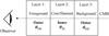 |
Fig. 2 Sketch of the multilayer model of a LoS. Top: line of sight decomposed into three layers: the foreground, inner, and background layers. Bottom: inner slab (layer 2) surrounded by two outer slabs that share the same physical and chemical state. Each region has homogeneous physical and chemical conditions (noted θin and θou, respectively). |
3.1 Modeling a heterogeneous line of sight
We aim to model the emission from a dense core or a filament surrounded by translucent gas. To do this, we model each LoS as three successive layers starting from the observer as illustrated in the top part of Fig. 2: the foreground layer (layer 1), the inner layer (layer 2), the background layer (layer 3). The contribution from the Cosmic Microwave Background (CMB) is considered separately as it is not emitted by the ISM cloud. We nickname this specific multilayer structure “sandwich model” because the foreground and background layers are part of the same outer layer and share the same physical and chemical conditions (see the bottom part of Fig. 2). In contrast, the inner layer has physical and chemical conditions that are distinct from those of the outer layer.
Following Myers et al. (1996), we assume 1) that the line excitation is local and the level populations in a slab do not depend on the physical conditions of other layers, but 2) that the emission of one layer is absorbed by the layers located between it and the observer. In other words, we neglect the non-local radiative coupling between layers, and the scattering of line photons of the core by the envelope, that is, the absorption and reemission of line photons coming from the core. This is a good approximation for CO and for optically thin lines, but it will be less exact for very subthermal (Tex ≪ Tkin) optically thick lines. These assumptions are consistent with the escape probability radiative transfer method that is used to model the emission from each layer (see, e.g., van der Tak et al. 2007). This approximation allows us to easily decompose the contribution of the different layers to the observed spectrum.
The brightness temperature s at observed frequency ν can be written as
 (1)
(1)
where sL(ν) is the brightness temperature of the layer L ∊ {fore, inner, back} attenuated by the gas in front of it. For any layer L, it can be written as
![Mathematical equation: ${s_L}(v) = J\left( {{T_{{\rm{ex}},L}},v} \right)\left[ {1 - \exp \left( { - {{\rm{\Psi }}_L}(v)} \right)} \right]\exp \left( { - \mathop {\mathop \sum \nolimits^ }\limits_{L - 1}^{i = 1} {{\rm{\Psi }}_i}(v)} \right),$](/articles/aa/full_html/2024/12/aa51567-24/aa51567-24-eq9.png) (2)
(2)
where Ψi·(ν) is the opacity profile of layer i and the specific intensity of layer L, expressed in temperature units, is
 (3)
(3)
The constants h and k in Eq. (3) are the Planck and Boltzmann constants, respectively. The specific intensity of layer L, J(Tex, L, ν), is affected by the layer itself through the term [1 − exp (−ΨL(ν))], and by the gas of the layers separating the layer L from the observer through the term exp  . The excitation temperature Tex, L between the upper and lower energy levels is related to the ratio of the populations of these energy levels through
 (4)
(4)
where 𝑔up and 𝑔low are the degeneracies of the associated levels (Draine 2011, Chap. 7, Eq. (7.8)).
Each molecular transition provides a spectrum around the rest frequency νl of the emission line l in the source frame. When dealing with several molecular lines simultaneously, it is more convenient to consider opacity profiles as a function of velocity V rather than frequency ν. These are related through the Doppler effect expressed with the radio convention as
 (5)
(5)
where c is the velocity of light. Assuming that the distribution of the gas velocities, which results from turbulent and thermal motions, is a Gaussian, centered on the centroid velocity CV,L, and of velocity dispersion σV, L, we can express the opacity profile for layer L and line l as a function of the velocity as
![Mathematical equation: ${{\rm{\Psi }}_{l,L}}(V) = {\tau _{l,L}}\exp \left[ { - {{{{\left( {V - {C_{V,L}}} \right)}^2}} \over {2\sigma _{V,L}^2}}} \right],$](/articles/aa/full_html/2024/12/aa51567-24/aa51567-24-eq14.png) (6)
(6)
where τl,L is the optical depth at the center of line l for the layer L. We assume that the centroid velocity CV,L and velocity dispersion σV,L are identical for all molecular lines in this layer. They thus only depend on the layer L. The full width at half maximum (FWHM) is related to the velocity dispersion σV by
 (7)
(7)
Finally, as the lines observed in the ISM have narrow widths, we can assume that J(Tex,L, ν) ≈ J(Tex,L, νl). For the sake of readability, we hereafter note J(Tex, L, ν) as J(Tex, L) and ΨL(V) = ΨL.
In summary, the spectrum observed at the output of the simplified sandwich model can be written as
 (8)
(8)
with
![Mathematical equation: ${s_{{\rm{fore}}}} = J\left( {{T_{{\rm{ex}},1}}} \right)\left[ {1 - \exp \left( { - {{\rm{\Psi }}_1}} \right)} \right],$](/articles/aa/full_html/2024/12/aa51567-24/aa51567-24-eq17.png) (9)
(9)
![Mathematical equation: ${s_{{\rm{inner}}}} = J\left( {{T_{{\rm{ex}},2}}} \right)\left[ {1 - \exp \left( { - {{\rm{\Psi }}_2}} \right)} \right]\exp \left( { - {{\rm{\Psi }}_1}} \right),$](/articles/aa/full_html/2024/12/aa51567-24/aa51567-24-eq18.png) (10)
(10)
![Mathematical equation: ${s_{{\rm{back}}}} = J\left( {{T_{{\rm{ex}},1}}} \right)\left[ {1 - \exp \left( { - {{\rm{\Psi }}_1}} \right)} \right]\exp \left( { - {{\rm{\Psi }}_1} - {{\rm{\Psi }}_2}} \right),$](/articles/aa/full_html/2024/12/aa51567-24/aa51567-24-eq19.png) (11)
(11)
![Mathematical equation: ${s_{{\rm{CMB}}}} = J\left( {{T_{{\rm{CMB}}}}} \right)\left[ {\exp \left( { - 2{{\rm{\Psi }}_1} - {{\rm{\Psi }}_2}} \right)} \right] - J\left( {{T_{{\rm{CMB}}}}} \right),$](/articles/aa/full_html/2024/12/aa51567-24/aa51567-24-eq20.png) (12)
(12)
where the J(Tex) and Ψ terms depend on the line l, and the Ψ terms in addition depends on the velocity V, but J(TCMB) only slowly depends on the frequency. In these equations, we used the symmetry of the slabs to set Ψ1 = Ψ3 (see Fig. 2). Moreover, the contribution from the CMB has a different expression as compared to the other layers. The CMB is a continuum emission from a source located at an “infinite” distance from the observer. This CMB emission is thus absorbed by the inner and outer layers in front of it (i.e., J(TCMB) [exp (−2Ψ1 − Ψ2)]). However, the calibrated spectrum obtained with the IRAM-30m radiotelescope results from the subtraction of the observation toward a reference LoS devoid of signal coming from the source (named OFF-position) from the observation toward the ON-source LoS. Assuming that the CMB emission is homogeneous and isotropic on the sky, the signal from the OFF-source LoS only contains the CMB emission. Furthermore, we assume that the CMB along the OFF-source LoS is not affected by any absorption. The ON-OFF process thus effectively subtracts J(TCMB) from the observed line signal. We fold this into our model by subtracting J(TCMB) from the CMB contribution to the modeled line emission (i.e., sCMB in Eq. (12)). Finally, we use as CMB temperature TCMB ≃ 2.73 K (Mather et al. 1994). Appendix B generalizes this formalism to an arbitrary number of layers.
References of the rate coefficients used in this article to compute the collisional excitation.
3.2 Using the RADEX code to compute the emission and opacity of each layer
We used the non-LTE RADEX code (van der Tak et al. 2007) to compute the excitation temperature (Tex) and opacity (τ) for each layer and each line. RADEX allows one to compute large grids of models in reasonnable times. To do this, RADEX uses a local approach, namely the escape probability radiative transfer method, to derive the populations of the different energy levels of the chosen molecular species. The references of the collisional excitation rate coefficients are listed in Table 3. We assume that the collisional partners are molecular hydrogen for all species, plus electrons for the high-dipole moment species HCO+ and H13CO+ (Goldsmith & Kauffmann 2017). The detailed prescriptions for the ortho-to-para ratio of the molecular hydrogen and for the electron density can be found in Sect. 2.1 of Roueff et al. (2024).
We have chosen to use the escape probability for a static uniform sphere. A spherical geometry appears better suited than a plane parallel geometry, because it allows photons to escape in all directions, and molecular clouds have a complex self-similar structure. In the chosen multilayer model, the velocity field is independently fitted in each layer and the layers are not radiatively coupled (i.e., the radiation field of a layer does not contribute to the level population of the gas in another layer). Therefore, we have chosen to consider each layer as a uniform medium. Using the expanding sphere geometry is less appropriate because this physical description requires no discontinuity for the centroid velocity between the layers. The expanding sphere model also implicitly assumes that the outer layer has a larger velocity dispersion than the inner layer because the expansion velocity field reaches higher values further away from the center. For a single-layer model, the influence of the choice of the escape probability law has been discussed by van der Tak et al. (2007). At low column densities, the uniform sphere model and the expanding spherical model lead to similar emergent intensities within about 10% while the plane parallel slab predicts higher line opacities and intensities. The difference is more significant at high column densities. This means that the choice of the escape probability law impacts the estimation of the physical conditions in a systematic way, but the difference between the estimations remain moderate (less than 50% for the density) for lines with low to moderate opacities (less than ~10). Anyway, the proposed method can be used with another choice of the escape probability, depending on the science context.
3.3 Estimated input parameters
For each species and each layer, the physical conditions are characterized by five unknown parameters: the kinetic temperature (Tkin), the volume density of molecular hydrogen  , the column density (N) of the considered species, the velocity dispersion (σV) expressed as a full width at half maximum (FWHM), and the centroid velocity (CV). Since the foreground and background layers are part of the same outer layer, they are characterized by the same five parameters. For each species, the sandwich model is therefore characterized by ten unknown parameters,
 (13)
(13)
We assumed that the five species are co-located inside each layer. The species thus share the same Tkin,  , CV, and FWHM per layer.
Constraining the column density of each species in each layer is complex because we only have one or two transitions per species. On the one hand, estimating all these column densities simultaneously is inefficient because there is not enough information to get accurate estimations. On the other hand, Roueff et al. (2024) show that fixing the ratio of column densities can bias the estimation of both the column densities and the other physical parameters such as the volume density when the injected constraints are invalid. To work around this issue, we discuss in Sect. 4 the choices of chemical assumptions made to decrease the number of fitted parameters.
3.4 Noise model
A noise model is required 1) to quantify the precision of the estimates, and 2) to derive the maximum likelihood estimator (MLE), which is used to fit the data. We design two slightly different noise models to meet the specific needs of each goal. From the first perspective, we take all noise sources into account in order to avoid underestimating the achievable precision (i.e., estimating too small error bars). In particular, our model takes into account not only the thermal additive noise, but also a calibration multiplicative noise that has a significant effect at high S/N (see Einig et al. 2023). However, when deriving the MLE, we omit the calibration multiplicative noise because Roueff et al. (2024) observe that taking it into account leads to correct results on Monte Carlo simulations, but poorer and inconsistent fits on actual data. They suggest that, in the case of real data, this additional flexibility of the fit is used to deal not only with calibration errors but also with model misspecifications, the latter effect being more significant than the former one. We now detail the full noise model used to quantify the precision on estimates. An observed spectrum xl for line l is a realization of the signal (noted sl) from Eq. (8) regularly sampled in velocity affected by an additive thermal noise bl and a multiplicative calibration noise c
 (14)
(14)
The additive noise bl is drawn from a centered Gaussian distribution with standard deviation σb,l, whose typical values are listed in Table 1. The calibration noise is drawn from a Gaussian distribution of mean 1.0 and standard deviation σc,l with
 (15)
(15)
The value quoted at 3 mm was estimated on the ORION-B dataset in Appendix D of Einig et al. (2023).
3.5 Saturation of the S/N during the fit
Our proposed estimate  of the vector of unknowns θ is obtained by minimizing the negative log-likelihood (NLL):
![Mathematical equation: $\hat \theta = \arg \mathop {\min }\limits_\theta [ - \log {\cal L}(\theta )],$](/articles/aa/full_html/2024/12/aa51567-24/aa51567-24-eq27.png) (16)
(16)
where
 (17)
(17)
In this equation, xl and sl are the observed and modeled spectra for line l, and  is the associated noise level. The NLL, − log ℒ, is a function of the physical input parameters θ, and we search for the value
  that minimizes it. Following Roueff et al. (2024), we only take into account the additive thermal noise in this expression. Indeed, implementing a MLE that takes into account the calibration noise leads to better performances on Monte Carlo simulations, especially when the S/N is high. However, we observe that it results on actual data in artificially large calibration factors to compensate for the oversimplified model assumptions, and thus in unrealistic estimations of the physical and chemical parameters (see Sect. 3.4).
We also saturate the peak S/N of all lines to a value of ten by adjusting the σb,l value in the likelihood function when needed. This saturation ensures that the HCO+ isotopologues have similar weights in the NLL as the CO isotopologues and thus significantly contribute to the estimation of the parameters. This saturation is needed because the use of broadband receivers means that the integration time is the same for all lines, resulting in different S/N for lines of different intensities. We are thus limited by the line that has the minimum S/N, that is the H13CO+ (1 − 0) line in our case. Figure 3 compares some observed spectra with their saturated noise versions. This figure illustrates the potential effect of the S/N saturation on the line profiles. We actually just adjust the σb,l value during the fit without changing the data themselves. In each panel, the top left and right numbers give the relative weight of a difference of 1 K in any given channel, that is,
 (18)
(18)
on the fit χ2 value before and after the S/N saturation, respectively. Before the saturation (left numbers), the CO isotopologues completely dominate the variations of the χ2. In contrast, after saturation (right numbers), the HCO+ isotopologues can significantly influence the variations of the χ2.
3.6 Constrained optimization
Compared to Roueff et al. (2024), the challenge in this study is to estimate about twice as many parameters by going from a homogeneous model to a heterogeneous one. To deal with this challenge, our optimizer starts with a grid search followed by a gradient descent algorithm. The grid of RADEX models is computed once and for all, while RADEX is run on the fly to evaluate the line models during the gradient descent. In addition, we chose to optimize the likelihood under the constraint that the column density ratios can vary within some intervals based on a priori astrophysical knowledge. In our implementation, the column density ratios are estimated within these constraints on abundance ratios during the grid search with a finite resolution of 0.05 in the logarithm of the abundance ratio (that is a factor of 1.12 in the abundance ratio). The column density ratios are then fixed during the gradient descent to the optimum value found during the grid search. This choice allows us to regularize our gradient, and thus to avoid convergence issues that occur when trying to apply a gradient descent to refine the estimations of the column density ratios. Indeed, the more unknowns, the higher the probability of obtaining singular Fisher matrices. Appendix C details this optimization process.
3.7 Removing inaccurate estimations with the Cramér-Rao bound
Once the fit has converged (i.e., after the grid search and the gradient descent), we filter out estimations with too large [−σ, +σ] confidence intervals. It happens that the square root of the Cramér-Rao bound (CRB) provides a lower bound on the standard deviation of estimated parameters for any unbiased estimators (Garthwaite et al. 1995). Mathematically speaking,
![Mathematical equation: $\sigma \left( {\widehat {{\theta _i}}} \right) \ge [CRB(\theta )]_{ii}^{1/2}{\rm{with}}\quad CRB(\theta ) = I_F^{ - 1}(\theta ),$](/articles/aa/full_html/2024/12/aa51567-24/aa51567-24-eq32.png) (19)
(19)
where IF is the Fisher information matrix defined by
![Mathematical equation: $\forall (i,j)\quad {\left[ {{I_F}(\theta )} \right]_{ij}} = \left[ {{{\partial \log {\cal L}({\bf{\theta }})} \over {\partial {\theta _i}}}{{\partial \log {\cal L}(\theta )} \over {\partial {\theta _j}}}} \right].$](/articles/aa/full_html/2024/12/aa51567-24/aa51567-24-eq33.png) (20)
(20)
In the previous equation, 𝔼 is the statistical expectation among the different realizations of x, defined in Eq. (14). As in Roueff et al. (2024), and since the true value of θ is unknown, we compute  instead of CRB(θ) to provide reference precisions of our estimations. Therefore, if
  is the estimate of θi ∊ θ (see Eq. (13)), we only retain
  for LoSs that comply with
 (21)
(21)
where Pther is the thermal pressure. When computing these CRB reference precisions, we take into account both the thermal and calibration noises to avoid underestimating the credibility interval (see Sect. 3.4). In the previous section, we have noted that some abundance ratios are only estimated during the grid search within astrophysically chosen fixed bounds, in order to stabilize the optimization problem. As the estimated abundance ratios are constrained within 12%, we simply neglect the increase of uncertainty due to this procedure. We therefore only have access to the accuracy on the estimation of one column density per layer with a Fisher information matrix of size 10 × 10, and we have no access to the accuracy on the estimation of the ratio of the column densities.
The gradients required to calculate the Fisher matrix and the CRB for any multilayer model, including the sandwich model, are given in Appendix D.
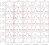 |
Fig. 3 Comparison of five observed spectra (black histograms) and the same ones plus the required amount of noise to saturate their peak S/N to ten (red histograms). The positions of the spectra are marked on Fig. 1 and listed in Table 2. Each row corresponds to a given species and transition, while each column corresponds to a given position. In each panel, the top left and right numbers give the relative weight of a difference of 1 K in any given channel on the fit χ2 value before and after the S/N saturation, respectively. The 12CO (1 − 0) and H13CO+ (1 − 0) lines were observed with a resolution about 5 times coarser than the other lines. When the peak S/N is lower than 10, the red spectrum is hidden under the black one. |
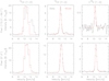 |
Fig. 4 Comparison of the observed (black) and modeled (red) (1 − 0) line of the 12CO, 13CO, and C18O species for two different LoSs. |
4 Physical and chemical assumptions
Having a large number of fitted parameters leads to large uncertainties. To reduce these uncertainties, we need to add constraints on estimated parameters with physical and chemical assumptions. Roueff et al. (2024) discuss in depth the possible occurrence of biases linked to these additional assumptions, and highlight that a single unreasonable constraint can dramatically bias the results. This section details and justifies the proposed hypotheses. First, we explain how we use the information carried by the 12CO (1 − 0) line of high opacity. Then, we compare the sandwich model with a simple homogeneous model consisting of a single layer, to illustrate the gain in signal reconstruction quality with the latter model. We continue by discussing the differences in the kinematic properties of the different layers, namely their velocity centroids and velocity dispersions. Finally, we introduce the hypotheses on the chemical abundances in the inner and outer layers.
4.1 Specific treatment for the 12CO (1−0) line
Figure 4 compares the observed and modeled spectra of the (1 − 0) lines of the three main CO isotopologues for two lines of sight. The main difference between these LoSs is the existence of a second velocity component between 12 and 14 km s−1 that contributes more than 10% of the total integrated intensity of the 12CO (1 − 0) line and much less than this for the 13CO and C18O (1 − 0) lines. While the model does a correct reconstruction of the main velocity component for the 12CO (1 − 0) line when we only fit the peak intensity of this line, the second velocity component perturbs the fit when we try to fit the full 12CO (1 − 0) profile. Since at this stage our algorithm has not been designed to fit multiple velocity components, we thus fit only the 12CO (1 − 0) peak temperature as proposed by Roueff et al. (2024). Fitting multiple velocity components will be the subject of a forthcoming paper.
4.2 On the importance of a heterogeneous model
The simplest possible geometry is to assume a homogeneous cloud composed of a single layer emitting in front of the CMB. However, the maps of the line emission (see Fig. 1) suggest that the emission comes from gas with different physical conditions, at least along the LoSs toward filaments and dense cores. We therefore introduce a three-layer model to take into account this inhomogeneity while keeping the model as simple as possible.
In this section we compare the integrated intensity computed on the data with that derived from the molecular line fitting with two different models. The first one is a homogeneous model described with
 (22)
(22)
The second one is a three-layer model described with
 (23)
(23)
The components used in these equations are defined in Eq. (9) to (12).
To simplify the comparison, we kept in each experiment the same fixed relative abundances, defined by using the following isotopic ratios for Orion 12C/13C= 63, 16O/ 18O= 510, and N(HCO+)/N(H2)=3 × 10−9 and N(13CO)/N(H2) = 2.3 × 10⁻⁶ (Gerin et al. 2019; Roueff et al. 2024, and references therein). Those give
 (24)
(24)
We refer to these column density ratios collectively as “basic” in the remainder of this work. In contrast, the centroid velocities, velocity dispersions, column densities, kinetic temperatures, and volume densities were estimated independently for the inner and outer layers.
Figure 5 compares the reconstruction of all the line profiles for the best fits obtained with either the homogeneous or the sandwich model. The total integrated line is plotted as a function of the visual extinction between 10 and 27 mag, where the probability of having different gas components along a single LoS is high. Intensities are averaged over all pixels that belong to a 1 mag sliding window of the visual extinction. The colored areas around the relative error curves show the associated standard deviations for all the pixels belonging to the sliding window. The vertical width of this ±σ-interval mostly decreases from low to high visual extinction because the number of pixels quickly decreases with AV.
The first obvious feature in Fig. 5 is that the sandwich model better reconstructs the line total integrated intensities than the homogeneous model. This is expected since the number of fitted parameters doubles from 5 to 10 when going from a homogeneous to a sandwich model. More interestingly, the sandwich model better reconstructs the lines that mostly originate from one type of medium with specific physical conditions: either translucent or dense and cold gas. The most striking example is the H13CO+ line whose relative error decreases from ~ − 80% to less than −25% for AV > 15 mag. The second example is the C18O (2 − 1) line whose typical relative error decreases from ~ −20% to less than ~10% over the plotted AV range. The second clear feature is that the sandwich model allows to decrease the intensities of the lines that are known to be optically thick (namely 12CO(1 − 0) and HCO+ (1 − 0)) and thus mostly sensitive to the external layer, while it increases the intensity of the optically thinnest line (e.g., H13CO+ (1 − 0)). Finally, the sandwich model becomes unbiased (i.e., its relative error is compatible with zero within the ±σ-interval) for large ranges of AV and for many lines. The most obvious example is the 13CO (2 − 1) line. Whatever the AV range, the absolute value of the relative reconstruction error almost always remains below 10%, a value consistent with the fact that we saturate the peak S/N to 10. Hereafter, we only discuss variants of the sandwich model.
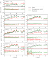 |
Fig. 5 Comparison of the reconstruction of all integrated line intensities for the best fit obtained with either a homogeneous (in red) or a simple sandwich model (in green). The integrated line intensity or peak temperature are plotted as a function of the visual extinction (AV). More precisely, the integrated line intensities (zero-order moment) or peak temperature are averaged over all the pixels whose visual extinction belongs to the [AV − 0.5, AV + 0.5] mag interval, where AV is plotted on the x-axis of the panels. The lack of values for AV ∈ [23, 24] mag results from the fact that there is no pixel in this range of AV over the studied field of view. In each panel, the top one shows the line integrated intensity or peak intensity, while the bottom one shows the reconstruction relative error in percentage. The colored areas on the relative error panels show the standard deviation over all the pixels that belong to the 1 mag-AV sliding window. The horizontal dashed line indicates a perfect reconstruction. While the simple sandwich model already better fit the data than the homogeneous model, the reconstruction will still be improved by refining the assumptions. |
4.3 On the importance of having independent centroid velocities to reproduce the spectrum asymmetries
A straightforward way to decrease the number of fitted parameters would be to use the same velocity distribution (centroid velocity and velocity dispersion) for the inner and outer layers. However, it is well known that the lines mostly tracing the dense and shielded gas (e.g., the C18O lines) are narrower than lines (e.g., the 12CO lines) probing the surrounding lower density, warmer, and more turbulent gas. This result is for example highlighted by Orkisz et al. (2019); Roueff et al. (2021); Gaudel et al. (2023). We here explore the importance of estimating independently the centroid velocities for the inner and outer layers. To do this, we compare the reconstruction of the spectra for the LoS B that shows asymmetric line profiles for, e.g., the HCO+ (1 − 0) line (see Table 2 and Fig. 3).
Figure 6 shows the fit of the 13CO (2 − 1) and HCO+ (1 − 0) lines for a sandwich model with the same centroid velocity for all the layers (top row) or with independent centroid velocities for the inner and outer layers (bottom row). The conditions for the fit of the other parameters are unchanged between these two experiments. In particular, the centroid velocity for each layer is identical for the seven fitted lines, and the column density ratios are fixed to their basic values listed in Eq. (24).
Fitting independently the centroid velocities of the inner and outer layers better reproduces the wings of the 13CO (2 − 1) line, explaining the decrease by more than a factor of two of the χ2 value for this line. But, more importantly, it is the only way to reproduce the large asymmetry of the HCO+ (1 − 0) line. Indeed, when using the same centroid velocity for all layers, the contribution of each layer shows a symmetrical profile. In contrast, allowing the simultaneous fit of the outer and inner centroid velocities delivers a symmetrical profile contribution of the foreground layer (red spectrum), and asymmetrical ones for all other layers (inner, background, and CMB). These asymmetrical line profiles are not just the result of adding symmetrical components shifted in velocity. Instead, marked asymmetries mainly result from the absorption of the intrinsically symmetrical emission term (J in Eq. (3)) of one layer by the velocity-shifted absorption of another layer in front of it. Taking into account different centroid velocities for the inner and outer layers therefore allowed us to model this coupling between emission and absorption.
Table 4 compares the fitted parameters for the inner and outer layers for these two experiments. The differences are of the order of 10%, except for the volume densities of the inner and outer layers, which increase by 0.05 to 0.1 dex (12 to 25%). When comparing the homogeneous model to the sandwich model in Sect. 4.2, the centroid velocities of the inner and outer layers are fitted independently. This is probably a reason why the HCO+ (1 − 0) integrated line profile is much better reconstructed with the sandwich model than with the homogeneous model.
Hereafter, we only discuss models where the centroid velocities for the inner and outer layers are independently estimated.
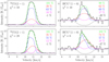 |
Fig. 6 Comparison of the data and the fit of the sandwich model when either the centroid velocities of all layers are assumed to be identical (top row) or they can have different values in the inner and outer layers (bottom row). The left and right columns show this comparison for the 13CO (2 − 1) and HCO+ (1 − 0) lines, respectively. These spectra correspond to the LoS B (see Table 2). Data and fitted spectra are shown in black and green lines, respectively. The contributions of the different layers are shown as colored lines: red for the foreground layer (see Eq. (9)), blue for the inner layer (see Eq. (10)), pink for the background layer (see Eq. (11)), and dashed black for the CMB (see Eq. (12)). |
Fitted parameters when assuming that the inner and outer layers have the same or different centroid velocities and velocity dispersions.
4.4 On the importance of fitting the N(C18O)/N(13CO) column density ratio
Roueff et al. (2024) show that it is in principle better to avoid constraining the column densities of the studied species because this lowers potential biases. However, fitting here one column density per species and per layer would imply to estimate ten additional parameters (five species for the inner, and five for the outer layers). Such a fit would lead to large uncertainties because of the limited number of measured transitions for the different species. We therefore search for the most suitable chemical hypotheses for the Horsehead nebula to limit the number of fitted column densities.
We start from the experiment described in Sect. 4.2, namely, fitting a sandwich model with column density ratios following the basic abundance ratios given in Eq. (24). While the relative error on the integrated intensity is within ±10% for the 13CO and C18O lines for AV > 10 mag, the fit almost systematically underestimates the integrated intensity of the 13CO lines, and overestimates that of the C18O lines, i.e., the relative errors are anticorrelated for these two species (see the green curves of Fig. 5). This behavior that is more salient for the (1 − 0) lines, questions the value chosen for the basic column density ratio. We therefore carried out a series of experiments in which we refitted the spectra over the whole field of view for several values of the N(13CO)/N(C18O) ratio. For each pixel, we thus obtained 14 solutions for which the only difference is the value of the N(13CO)/N(C18O) ratio that goes from 5.62 to 25.12 in multiplicative steps of 1.121. In all of these experiments, we used the same value of the N(13CO)/N(C18O) ratio for both the inner and outer layers. As the solutions are obtained with the same data and same number of fitted parameters, comparing the NLL values (Eq. (17)) allowed us to select the best value of the N(13CO)/N(C18O) ratios for each pixel. As this manual approach is akin to a fit of the column density ratio, we incorporated it in the grid search step of the proposed MLE estimator for the remainder of this work.
Figure 7 compares the reconstruction of the 13CO and C18O line integrated intensities obtained with either a fixed basic N(13CO)/N(C18O) ratio for all pixels, or an estimated N(13CO)/N(C18O) ratio per pixel. The reconstructed integrated intensities are shown as a function of the visual extinction in the [4, 13] magnitude range, where we expect deviations of the N(13CO)/N(C18O) ratio from its basic value because of the selective photodissociation of C18O combined with enrichment of 13CO by isotopic fractionation (Langer et al. 1984; Kong et al. 2015). We do not show the results for lower AV values because the C18O lines have either very low S/N or are not detected at all, implying that the data are no longer sensitive to the N(13CO)/N(C18O) ratio. We find that fitting the N(13CO)/N(C18O) ratio considerably decreases the negative (resp. positive) bias when reconstructing the 13CO (resp. C18O) integrated line intensity. In particular, the (2 − 1) lines now have unbiased fitted integrated intensities.
Hereafter, we continue to fit the N(13CO)/N(C18O) column density ratio.
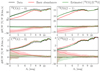 |
Fig. 7 Comparison of the reconstruction of the 13CO and C18O line integrated intensities for the sandwich model fit obtained with either a fixed relative abundance of [13CO]/[C18O] (in red) or an estimated relative abundance of this ratio (in green). The figure layout is similar to Fig. 5. |
4.5 On the importance of allowing the N(HCO+)/N(13CO) column density ratio to vary in the outer translucent layer
In this subsection we first show that fixing the value of the N(HCO+)/N(13CO) column density ratio to its basic value listed in Eq. (24) leads to an ambiguity in the estimation of the volume density of the inner layer because the NLL shows two local minima of similar depth around 104 and 106 cm−3 . The estimator thus oscillates between these two values depending on the noise level. We therefore considered fitting the column densities of the HCO+ isotopologues in addition to the column densities of the CO isotopologues (see Sect. 4.4). However, fitting the column densities of both HCO+ and H13CO+ for all lines of sight will result in a high variance because of the higher number of unknowns and relatively low S/N of the HCO+ isotopologue lines. As a compromise, we thus propose 1) to take N(HCO+)/N(12CO)= N(H13CO+)/N(13CO) for the outer layer, as this is plausible for translucent gas following the analysis described in Sect. 4.5.2, and 2) to keep the basic abundance ratios in the inner layer made of colder, denser gas.
4.5.1 On the impact of the N(HCO+)/N(13CO) value on the number of local minima of the NLL
The model described in Sect. 4.4 fits the column densities of 13CO and C18O, but it fixes the column densities of 12CO, HCO+ , and H13CO+ by assuming that they have constant abundances relative to 13CO. Fitting all the lines of sight toward the Horsehead nebula with this model shows that the fit oscillates between two solutions for the inner layers: one with a density around 104 cm−3, and another one with the density around 106 cm−3 . This situation often happens when fitting low-J lines of CO and HCO+ isotopologues (see, for instance, Fig. 10 Roueff et al. 2024). As previous studies of the Horsehead nebula suggest that the volume density should be about ~2 × 105 cm−3 (Pety et al. 2005; Habart et al. 2005; Goicoechea et al. 2006; Pety et al. 2007), it is tempting to limit the range of volume densities to this upper value, but it is better to solve this issue based on chemical assumptions.
To understand why the fit fluctuates between two values of the volume density separated by two orders of magnitude, we have selected one line of sight for which the volume density of the inner layer is fitted to 106 cm−3 , namely LoS A. The top row of Fig. 8 shows the variations of the NLL as a function of the volume density of the inner layer, while all other estimated parameters remain fixed at the values found during the fit. The minimum of the NLL for this LoS happens at 2 × 106 cm−3 , but a second local minimum occurs at 5 × 104 cm−3 with only an increase of the NLL of 14%. The NLL of all optically thick (12CO, 13CO, and HCO+) lines show a decrease followed by a plateau when the volume density increases. A plateau implies that the line intensity is no longer sensitive to the volume density of the inner layer. The NLL of the two optically thin lines (C18O and H13CO+) show one or two more or less deep wells at various relatively low  values followed by a plateau at higher
  values. Only the (1 − 0) lines of HCO+ and H13CO+ have not yet reached the NLL plateau at
  ~ 104 cm−3. The variations of the NLL of these two lines above 104 cm−3 thus discriminate between the fitted
  values. This is consistent with the higher critical density of the HCO+ isotopologue lines (~105±0.3 cm−3) than those of the CO isotopologue lines (~103.3±0.2 cm−3 , see Tables 6 and 7 of Roueff et al. 2024).
Next, we decreased the abundance of HCO+ with respect to 13CO by a factor of two. The bottom row of Fig. 8 shows the variations of the NLL as a function of the volume density in this case. The NLL variations are significant only for the HCO+ (1 − 0) line, which now shows a deep well aligned with the much more optically thin H13CO+ (1 − 0) line at  ~ 1.8 × 104 cm−3. This translates into a marked well of the total NLL at the same value of
  . For
. For  ≳ 104 cm−3, the fitted value of
  is governed by the variations of the NLL of the (1 − 0) lines of the two main HCO+ isotopologues. Varying the abundance of HCO+ relative to 13CO yields or lifts a degeneracy of the solution for
  . It is thus important to fit the column density of HCO+ and H13CO+ in order to avoid biasing the value of the fitted volume densities. However, fitting the column density of HCO+ and H13CO+ in both layers increases considerably the number of unknowns to be estimated. We thus turn to chemical considerations to assess whether we can make a more relevant hypothesis than assuming constant abundances of HCO+ and H13CO+ relative to 12CO and 13CO respectively.
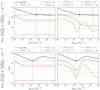 |
Fig. 8 Comparison of the variations of the NLL as a function of the volume density of the inner layer for the LoS A. We used a sandwich model where N(13CO) and N (C18 O) were fitted, while the column densities of 12CO, HCO+, and H13CO+ were computed assuming fixed abundances relative to 13CO. The top and bottom rows show the NLL variations for two values of N(HCO+)/N(13CO) varying by a factor of 2.0. The left panel shows the NLL variations for the 12CO and 13CO lines, while the right panel show that of the C18O, HCO+, and H13CO+ lines. In both panels, the black plain lines shows the variations of the NLL when fitting all the lines. The top row shows two local minima at similar NLL values while the bottom row only shows one local minimum. The vertical and horizontal black dotted lines intersect at the lowest NLL value, indicated by the red circle, and at the second local minimum that is indicated by the black circle, when it exists. |
4.5.2 The N(HCO+)/N(12CO)=N(H13CO+)/N(13CO) hypothesis for the outer layer
The outer layer consists primarily of translucent gas with moderate temperatures in the presence of ultraviolet radiation. The forward fractionation reaction involved in the
 (25)
(25)
equilibrium is moderately efficient in lukewarm gas (Langer 1977). The left-to-right reaction is privileged when the gas kinetic temperature is ≲ 35 K because the right-to-left reaction is endothermic. Moreover, selective photodissociation tends to destroy more efficiently 13CO and C18O than 12CO. The actual chemical balance between these two opposite trends requires a detailed radiative transfer treatment which can be performed for example by the Meudon PDR code.
We now discuss the main formation and destruction pathways for HCO+ and H13CO+. Both molecular ions are essentially formed through two reactions that involve 12CO+ or 13CO+ . The first reaction,

has the same reaction rate coefficient for both isotopologues, k = 7.5 × 10⁻¹⁰ cm3 s−1 (Scott et al. 1997). The second reaction also have the same reaction rate coefficient, k = 1.7 × 10⁻⁹ cm3 s−1 (computed with the Langevin approximation Gioumousis & Stevenson 1958):

In addition, both molecular ions are principally destroyed through dissociative recombination with a reaction rate coefficient of 1.4 × 10⁻⁶ cm3 s−1 at 30 K (Hamberg et al. 2014):

With an electronic fraction of about 10−4–10−6 in translucent environments, as found in Bron et al. (2021), the destruction rate of HCO+ and H13CO+ is in the  range.
The HCO+ and H13CO+ destruction rates via the isotopic exchange reactions (Mladenović & Roueff 2014),
 (26)
(26)
have a significantly smaller value of a few  , as the forward reaction rate coefficient is 6.5 × 10⁻¹⁰ cm3 s−1 at 30 K, and the relative abundance of 12CO is a few 10−5. In the conditions where the main formation channel of HCO+ and H13CO+ is via the reactions of 12CO and 13CO with
  , we obtain the HCO+/H13CO+ = 12CO/13CO relation at steady state.
We checked how the 0D models used in Bron et al. (2021), which sample a range of densities and illuminations appropriate to translucent conditions, probe the N(12CO)/N(HCO+) ratio as a function of the N(13CO)/N(H13CO+) ratio. We introduced selective photodissociation effects in CO isotopologues by introducing different approximate analytical expressions of the photodissociation rates obtained from Fig. 9 of Visser et al. (2009), in the chemical network, including the various isotopic exchange reactions of carbon and oxygen. Given these assumptions, we have computed 4000 models that uniformly sample the parameter space appropriate to translucent environments as in (Bron et al. 2021), and filtered the simulations that lead to N(13CO) < 1014 cm−2. Figure 9 shows the joint histograms of N(HCO+)/N(12CO) vs N(H13CO+)/N(13CO) in log-space for the 3224 remaining models. The models sample more than three orders of magnitude for these abundance ratios but the histogram is relatively well approximated by a line of slope one going through the basic abundance ratio listed in Eq. (24).
For the sake of clarity, Table 5 compares the chemical assumptions and their implications for column density ratios for the two main chemical models presented so far.
Assumptions on column density ratios or relative abundances for the basic and improved sandwich models.
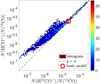 |
Fig. 9 Joint histogram of N(HCO+)/N(12CO) versus N(H13CO+)/N(13CO) in log space for the 3224 chemical models sampling various physical conditions in translucent gas. The red circle shows the ratio derived from the basic abundances listed in Eq. (24). The dashed blue line has a slope of 1.0. |
4.5.3 Intermediate summary
In the remainder of this study, we only consider the following hypotheses that we refer to as the “improved” model. We fit the peak intensity of the 12CO (1 − 0) line and the line profiles of all the other lines. We consider a sandwich model (foreground, inner, background, and CMB) in which the foreground and background layers (collectively called the outer layer) share the same physical and chemical properties. In contrast, the physical properties (velocity centroid and velocity dispersion, kinetic temperature, and volume density) are estimated independently for the inner and outer layers. In each layer, all the lines share the same physical and chemical properties, that is, their emissions are considered co-located inside each layer.
From the chemical viewpoint, the inner and outer layers are modeled differently. In the inner dense layer, we estimate the 13CO and HCO+ column densities, and we derive the column densities of the other species by assuming that they scale with the elemental abundances of the corresponding carbon and oxygen isotopes, that is,
 (27)
(27)
 (28)
(28)
 (29)
(29)
In the outer translucent layer, we fit the column density of 12CO, 13CO, C18O, and HCO+ , and we deduce the column density of H13CO+ with the constraint
 (30)
(30)
We thus have 14 parameters to estimate: four physical parameters  , FWHM) per layer plus four and two column densities for the outer and inner layers, respectively.
5 Results
Our goal in this section is two-fold. We first want to check whether the used hypotheses allow us to estimate chemical and physical parameters that are consistent with previous findings. Second, most of the previous results about the Horsehead pillar were derived with a single-layer model, while the sandwich model allows us to characterize the chemical and physical structure of the gas along the LoS. We first focus on the structure along the LoS (Sect. 5.1 and 5.2): We study whether the integrated intensity of the different lines is dominated by one of the three layers or whether it is distributed between the different layers. We search for the origin of the asymmetry of the line profiles. We compare the line excitation temperature with the CMB. We then look at the abundances of the CO and HCO+ isotopologues along the LoS as a function of H2 column density and far UV radiation field (Sect. 5.3): we try to quantitatively relate the variations of the abundances with known chemical processes such as photodissociation, isotopic fractionation, or freezing onto dust grains. Finally, we investigate the relationship of the derived physical parameters with the star formation activity (Sects. 5.4 and 5.5): we search for a kinematic signature of infall or expansion of the gas onto the filaments and dense cores. We discuss whether the molecular gas properties (kinetic temperature, volume density, and thermal pressure) are affected by the nearby presence of a PDR or of a young stellar object.
5.1 Contribution of the different layers to the integrated intensity
For each studied line, Fig. 10 shows 1) the relative error of the integrated intensity estimated by the model with respect to the observed value, integrated between 8.0 and 13.5 km s−1 (first column), and 2) the contributions of the different layers (foreground, inner, background, and CMB, from the second to the fifth column) to the line integrated intensity. While our estimator only fits the 12CO (1 − 0) peak intensity, we still provide the relative error and contributions of each layer to the integrated intensity of this line. We have filtered out sight-lines where the relative error on the integrated line intensity is larger than 40% or the visual extinction is lower than 3 mag for all lines, except for the faint H13CO+ (1 − 0) line where we used a threshold of 10 mag. The percentage listed in the top right corner of each panel is the mean±rms value computed over the selected sight-lines for the associated map. As expected, a negative contribution is ascribed to the CMB layer because of the ON-OFF observation procedure that implies the subtraction of a black body emission at 2.73 K as indicated in Eq. (8). Moreover, the sum of contributions of the layers to the integrated intensities can be larger than 100% when the estimated signal exceeds the observed integrated line intensity.
The integrated intensity of all the lines is reconstructed within 20% overall  . The rms of the relative error on the integrated intensity decreases when the S/N increases, except for the 12CO (1 − 0) line. The 13CO (2 − 1) and C18O (1 − 0) and (2 − 1) lines are reconstructed with much less bias (±1%) than the 12CO, 13CO, HCO+, and H13CO+(1−0) lines. The bias for the 12CO (1 − 0) line can be explained by the fact that we only use the peak temperature in the fit.
The contributions of the different layers to the integrated intensity depend much on the considered species. The 12CO (1 − 0) integrated intensity mainly comes from the foreground layer (85%) with a second contribution from the inner layer (22%), while the integrated intensity of the two C18O lines mainly comes from the inner layer (57%) with an approximately equal contributions from the foreground and background layers (~24% each). The 13CO lines have an intermediate behavior. The 13CO (1 − 0) integrated intensity comes from the foreground, inner, and background layers at approximately equal shares. The foreground layer contributes more than the background layer for the 13CO (2 − 1) line. This is consistent with the higher optical depth for the (2 − 1) line as compared with the (1 − 0) one.
The (1 − 0) line of the HCO+ isotopologues shows a very different behavior that is mostly related to the fact that its excitation temperature is close to the CMB temperature. While the subtraction of the CMB has a small effect on the CO isotopologues, it is significant for the HCO+ and H13CO+ lines and can lead to a significant negative contribution to the total integrated line intensity, beyond −50%. The foreground, inner, and background layers must therefore provide contributions significantly larger than the detected integrated line intensity to compensate, implying that the percentage of the combined layer contributions is larger than 100%. The inner layer contribution to the (1 − 0) line is about 50% for both HCO+ and H13CO+. However, the foreground contribution largely dominates the background contribution for the HCO+ optically thick line, while both layers have approximately equal contributions for the optically thin H13CO+ line.
Looking at the spatial distribution of the contributions for the 13CO and C18O lines, the inner layer contributes much more than the outer layers when the visual extinction is larger than 7 mag, and vice-versa. We relate this to the change of geometry of the Horsehead pillar that happens approximately at this visual extinction. Above 7 mag, the geometry is mostly face-on and the inner layer dominates for optically thin lines. Below 7 mag, the geometry becomes edge-on, and the contribution of the inner layer decreases and sometimes vanishes compared to that of the outer layers.
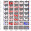 |
Fig. 10 Maps of the contributions of the different layers to the line intensity integrated between 8 and 13.5 km s−1. First column: relative error of the model with respect of the data in percentage. Second to fifth columns: contribution of the foreground, inner, background, and CMB layers to the line integrated intensity in percentage of that measured on the data. Each row corresponds to a given line: from top to bottom, 12CO (1 − 0), 13CO (1 − 0) and (2 − 1), C18O (1 − 0) and (2 − 1), HCO+ (1 − 0), and H13CO+ (1 − 0). The percentage on the top center of each panel is the mean±rms value computed over the associated maps. Positive and negative relative errors or contributions are shown in red and blue, respectively. |
5.2 Contribution of the different layers to the spectra
To get a better understanding of how the different layers contribute to the observed spectra, Figs. 11, H.1, and H.2 show the modeled decomposition of spectra selected around the dense cores 1, and 2, and then in the outskirts of the Horsehead nebula, respectively. In all cases, the background emission is attenuated by the inner layer in its foreground. Hence, the contribution of the background layer to the emergent spectra mostly matters in the line wings. Similarly, the emission from the inner layer is absorbed by the foreground layer, and this radiative interaction allows one to fit the asymmetries of the profiles of the optically thick lines of 12CO, 13CO, and HCO+.
Figure 11 first shows the decomposition at the peak of the H13CO+ emission (DC 1) for the dense core located at the top of the Horsehead. Positions A and B are two nearby LoSs that have already been used to justify some of the assumptions made in our modeling (see Sects. 4.3 and 4.5). Positions C and D are located at the edge of the dense core away from the σOri star that photo-excites the Horsehead PDR, where the HCO+ (1 − 0) peak emission abruptly decreases from above 3.5 K to below 2.5 K on Fig. 1. The inner layer emission contributes the most to the integrated line intensity near the dense core projected center (e.g., positions 1 and A). This is true even for the 12CO (1 − 0) line where the inner emission contributes about 20% of the total integrated line intensity. When going further away from the dense core center (positions C and D), the inner layer continues to provide the dominant contribution for the optically thin C18O lines, while the contributions from the foreground and background layers have either similar integrated line intensities as that from the inner layer, or even dominate for the 12CO or HCO+ lines. Position B seems to be an intermediate case.
Figure H.1 shows the decomposition at the peak of the H13CO+ emission (DC 2) for the dense core located in the neck of the Horsehead. Positions E and G are located where the H13CO+ (1 − 0) peak emission abruptly decreases from above 0.25 to below 0.10 K. Position F is extensively studied in Roueff et al. (2024). Position H is located at a LoS where the C18O(1 − 0) emission drops below 3 K. In contrast with the analysis of the previous dense core, the inner layer contributes less to the overall integrated line intensity of the optically thick lines at position 2 near the dense core projected center than at position F located further away. Positions E and G at the edge of the dense core shows a strong asymmetry of the most optically thick lines for which the foreground and background contributions may even dominate the integrated line intensity. This effect is less prominent for the position H located at the transition between the C18O filament and its environment.
Figure H.2 shows the decomposition for LoSs located at the outskirt of Horsehead pillar. There is an embedded young stellar object at position I. Positions J and K are located in the Horsehead mane and muzzle where the C18O(1 − 0) peak intensity is still ~2K, but the H13CO+ (1 − 0) is not clearly detected anymore. Finally, positions L and M are located where the 13CO (1 − 0) peak intensity drops below 10 K. Except for position I that has a similar behavior as the positions near the dense core 1, positions J to M have no clearly detected H13CO+, and faint HCO+ and C18O lines. The optically thick lines of HCO+ and 12CO at the K and L positions have inner and outer contributions whose radiative interaction (absorption) almost cancel each other. This is accompanied by an inversion of the centroid velocities of the two components (see Sect. 5.4). Finally, position M shows a spectral decomposition where the fit seems to have inverted the properties of the inner and outer layers as compared with the rest of the map. The integrated line intensity is completely dominated by the outer layers, and the associated linewidth is much wider than for the previous positions. We interpret this as the transition between the face-on and edge-on geometry at the outskirts of the Horsehead pillar. In the edge- on geometry the chemistry is better represented by assumptions enforced in the outer layer. Position M is a clear example of the strong coupling between the chosen chemical hypotheses as a function of the geometry and the inferred kinematics properties.
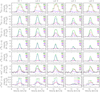 |
Fig. 11 Modeled decomposition of some spectra around the first dense core. Each column corresponds to the spectra for one of the lines of sight listed in Table 2. Each row corresponds to a given line, from top to bottom: 12CO(1 − 0), 13CO(1 − 0) and (2 − 1), C18O(1 − 0) and (2 − 1), HCO+ (1 − 0), and H13CO+ (1 − 0). We show the decomposition of the full spectrum of 12CO (1 − 0) even though we only used its peak intensity during the fit. In each panel, the data and model spectra are shown as the black and green histograms, respectively. The contributions of the foreground, inner, background layers are shown as the plain lines in red, blue, pink, respectively, and the CMB layer is displayed as the dashed black line. |
5.3 Chemical abundances
5.3.1 Relative abundances
Figure 12 shows the spatial distribution of ratios of different column densities derived for the outer layer. These ratios are normalized by the basic value derived from elemental abundances of carbon and oxygen isotopes (see Eq. (24)) and previous studies of the targeted molecules as explained in Sect. 4.2. By construction, these basic values are enforced in the inner layer, and N(HCO+)/N(12CO)=N(H13CO+)/N(13CO) in both layers (see Sect. 4.5).
The mean value of the N(13CO)/N(12CO) ratio in the outer layer is ~1.6 times the “basic” value used in the inner layer. Moreover, 13C+ is detected by Pabst et al. (2017), and the temperature remains moderate in the outer layer, as shown in Sect. 5.5. All this allows the forward reaction of the fractionation reaction (Eq. (25)) to predominate in the outer layer (see also Liszt 2007; Röllig & Ossenkopf 2013). The N(13CO)/N(12CO) ratio is also enhanced toward the DC 2 LoS, which is in line with the H13CO+ detection in that environment.
Two effects help explain the spatial variations of the N(C18O)/N(13CO) ratio in the outer layer. First, the abundance of 13CO is enhanced due to the C+ fractionation described above. Second, C18O is more easily photodissociated than 13CO (a process named selective photodissociation). Indeed, the shift between the C18O and 12CO pre-dissociated UV absorption transitions is significantly larger than the one between the 13CO and 12CO transitions. Shielding effect by 12CO are thus reduced for C18O with respect to 13CO. Both effects are important over most of the field of view, in particular for visual extinctions lower than 7 mag.
The spatial variations of the HCO+ abundance relative to CO are larger than those of the two other abundance ratios. The N(HCO+)/N(12CO) and N(H13CO+)/N(13CO) ratios are one to four times larger than the basic value toward dense core LoSs and two to ten times lower than this value for LoSs where 3 ≤ AV ≤ 7 mag. The HCO+ abundance relative to CO reaches values within a factor of two from the basic value in regions where AV is around 10 mag.
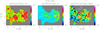 |
Fig. 12 Maps of the ratios of the column densities for the outer layer. These ratios have been normalized by the basic values established using the elemental isotopic ratios of carbon and oxygen (see Eq. (24)). By construction N(HCO+)/N(12CO) = N(H13CO+)/N(13CO) (see Sect. 4.5). Contours are drawn at visual extinctions of 3, 7, and 16 mag. |
5.3.2 Column densities and mean abundances relative to H2
For each species, Fig. 13 shows the inner, outer (foreground plus background), and total (inner plus twice outer) column densities, as well as its mean abundance along the LoS defined as
 (31)
(31)
where
 (32)
(32)
Following (Pety et al. 2017), we estimated the total column density of H2 from the “molecular” visual extinction (defined in Sect. 2 and Appendix A) as
 (33)
(33)
We have also added the ratio of column densities in the inner and outer layers, Nin/Nou ratio for each species in this figure to illustrate whether one layer dominates or whether the mean abundance results from just an average of both layers. Indeed, if we define the abundance of a species X with respect to H2 in the layer L as
![Mathematical equation: ${[X]_L} = {{{N_L}(X)} \over {{N_L}\left( {{{\rm{H}}_2}} \right)}},$](/articles/aa/full_html/2024/12/aa51567-24/aa51567-24-eq69.png) (34)
(34)
it is straightforward to show that
![Mathematical equation: ${{\langle X\rangle } \over {{{[X]}_{{\rm{in}}}}}} = {{1 + 2{{{N_{{\rm{ou}}}}(X)} \over {{N_{{\rm{in}}}}(X)}}} \over {1 + 2{{{{[X]}_{{\rm{in}}}}} \over {{{[X]}_{{\rm{ou}}}}}}{{{N_{{\rm{ou}}}}(X)} \over {{N_{{\rm{in}}}}(X)}}}}.$](/articles/aa/full_html/2024/12/aa51567-24/aa51567-24-eq70.png) (35)
(35)
In this equation, the mean abundance of species X converges to [X]in when Nou(X) ≪ Nin(X), and to [X]ou when Nou(X) ≫ Nin(X). The convergence rate depends on the value of the [X]in / [X]ou ratio.
The maps of the total column density for the three main CO isotopologues clearly show the filamentary structure inside the Horsehead pillar. From this viewpoint, they look more like the column density of the inner layer than that of the outer layer. This is consistent with the fact that the ratio of the inner and outer column densities is much larger than one for extinctions above 7 mag, and around or lower than one when 3 ≤ AV ≤ 7 mag. Even though the 12CO (1 − 0) line is highly optically thick, the simultaneous fit of different chemical species allowed us to recover reasonable column densities of 12CO for the inner layer.
In contrast, the maps of the total column density for the two main HCO+ isotopologues show a more balanced combination of column densities from the inner and outer layers, in agreement with the less contrasted maps of the ratio of the inner and outer column densities. For HCO+, the column density of the inner layer delineates the filamentary structure with a peak of the column density toward the dense cores. The map of the outer column density shows less structure. The total column density map of H13CO+ clearly shows higher column densities in the regions of higher extinctions. Overall the relative abundance seems to be somewhat higher along the LoSs toward dense cores and fairly constant elsewhere given the limited S/N of the line.
The most striking feature of the mean abundance maps is the depletion of the CO isotopologues toward the two dense cores. This is obvious for the dense core in the Horsehead neck. For the dense core at the top of the Horsehead, it is clearer for the mean abundance of 12CO than for those of 13CO and C18O. To quantitatively confirm these trends, Fig. 14 shows the joint histograms of the column densities and mean abundances as a function of the “molecular” visual extinction. We have fitted independently in each range of AV a power-law to the scatter plots of Ntot versus AV. We have used the CRB values to take into account the uncertainty on Ntot and we have assumed that the visual extinction are perfectly known. Appendix E explains the computation of the uncertainty on Ntot , and Appendix F details the fit algorithm. For the sake of reproducibility, the values of the fitted coefficients are listed in Table 6 and shown as the black lines in the third column of Fig. 14. The abundance of C18O with respect to H2 reaches 2.0 × 10⁻⁷ at the DC 1 position and 1.3 × 10⁻⁷ at DC 2. As the used “basic” abundance of C18O is 2.84 × 10⁻⁷, this implies depletion factors of 1.4 for DC 1 and 2.2 for DC 2. Such values are in agreement with abundances and depletion factors obtained in other studies of molecular cores. For instance, Tafalla et al. (2002) found a strong depletion of C18O in the inner regions of five Taurus starless cores (less than 100″ or 0.07 pc from their center) using a reference C18O abundance of 1.7 × 10⁻⁷. In a more recent study of four dense cores located in infrared dark clouds, Feng et al. (2020) also measure depletion factors of a few for C18O.
As the far UV radiation field plays an important role at least in the eastern part of the Horsehead pillar, Fig. H.3 shows the joint histograms of the column densities and mean abundances as a function of the G0/AV ratio. We use this ratio as a proxy of the ratio of the far UV field over the volume density that controls to first order the chemistry of PDRs. Using this proxy assumes that there is some relation between the volume and column densities.
The mean abundances of 12CO and 13CO increases up to a visual extinction of about 3 mag. At this visual extinction, they reach the values corresponding to the elemental abundance of the associated carbon isotope. For AV ≳ 7 mag depletion sets in, and the column density does not increase much anymore, which leads to a decreased abundance. The abundance of C18O increases up to AV ~ 7 mag, and then decreases. Looking at the G0/AV ratio, the column densities increase when G0/AV decreases from 15 to 1.5 ISRF mag−1, and then they remain mostly constant. When G0/AV ≤ 4.75 ISRF mag−1, the inner column density clearly dominates the column density budget. Above this value the total column density is dominated by the outer layer for 12CO and 13CO, but it remains dominated by the inner layer for C18O.
The column densities of the two HCO+ isotopologues studied increase more steadily with increasing visual extinction or decreasing G0/AV values. The associated mean abundances are quite scattered. Their typical values seem to be lower than the basic values (see Eq. (24)) by a factor between two and three (or between 0.3 and 0.5 dex). For both isotopologues, the total column density includes contributions from both layers.
Looking at the inner and outer column densities of the CO isotopologues as a function of G0/AV, we can distinguish another regime. For 1.5 ≤ G0/AV ≤ 4.75 ISRF mag−1, the column densities of CO isotopologues clearly decrease with increasing G0/AV in the inner layer, while they seem to saturate in the outer layer. The opposite behavior is seen for 4.75 ≤ G0/AV ISRF mag−1, namely the column densities of the CO isotopologues do not change much with increasing G0/AV in the inner layer, while the column densities of the outer layer decrease. This behavior may be caused by the increased photodissociation of the CO isotopologues in a higher far UV radiation field.
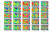 |
Fig. 13 Maps of the chemical properties for 12CO, 13CO, C18O, and HCO+, from top to bottom. The three first columns show the column densities for the inner, outer (foreground or background), and total (inner plus twice outer) column densities, while the last column shows the mean abundance, namely, the total column density divided by the H2 column density deduced from the visual extinction. The last column is the ratio of the inner by the outer column density. Contours are drawn at visual extinctions of 3, 7, and 16 mag. |
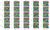 |
Fig. 14 Joint histograms of the molecular column densities, abundances, or their ratios as a function of the visual extinction for 12CO, 13CO, C18O, HCO+, and H13CO+, from top to bottom. The three first columns show the column densities for the inner, outer (foreground or background), and total (inner plus twice outer) column densities, while the last column shows the mean abundance, namely, the total column density divided by the H2 column density deduced from the visual extinction. The dashed vertical lines mark the visual extinction at 3, 7, and 16 mag. The red plain lines show the species basic abundance. The black lines show the piecewise power-law fits of the column densities within the AV ranges specified above (see Table 6) and the ±3σ intervals of the fits. These fits can be directly converted to an abundance vs visual extinction relation. |
Parameters of the piecewise power-law fits (log(Ntot) = α [log(AV) − log(AV)0] + β) for each studied species.
5.4 Kinematics
In Fig. 15, we compare the spatial distribution of the centroid velocity and velocity dispersion between the inner and outer layers. The centroid velocity of the inner and outer layers displays to first order an increasing gradient from north to south of the Horsehead. Hily-Blant et al. (2005) already described this behavior and interpreted this as a global rotation of the Horsehead pillar around its east-west axis.
We concentrate on LoSs where AV ≥ 7 mag. The difference of the centroid velocities for the inner and outer layers confirms that the centroid velocity of the outer layer follows that of the inner layer, shifted by about −0.25 km s−1. To check whether this shift is significant, we divide the absolute value of CV,in − CV,ou by its standard deviation computed as the square root of the CRB. We obtain that the centroid velocity difference is larger than the standard deviation for 90% of the lines of sight, and it is four times larger for 50% of the lines of sight, including those toward the dense cores. This suggests that the foreground layer moves toward the inner layer and away from the observer. This could hint to accretion of translucent gas onto the denser inner filament. However, the proposed model attributes the same centroid velocity to the foreground and background layers. A model that allows for the description of the infall or expansion motions along the LoS would mirror the centroid velocities of the foreground and background layers with respect to the inner layer one. More precisely, it would use different centroid velocities of the foreground and background layers with a velocity offsets of opposite signs with respect to the centroid velocity of the inner layer. This model variant will be tested in a forthcoming paper. In the meanwhile, we note that the background layer contributes little to the total integrated line intensity. Moreover, for the same LoSs (AV ≥ 7 mag), the velocity dispersion is about twice as large in the outer layer than in the inner one (~0.5 and ~0.25 km s−1, respectively). The outer layer thus appears more turbulent than the inner one, as might be expected when the gas becomes denser from translucent to dense gas through filamentary gas.
For LoSs where AV < 7 mag, an inversion of the centroid velocity shift and of the velocity dispersion ratio sometimes happens between the inner and outer layers (see, for instance, δx ∈ [1.5′, 3.0′] and δy ∈ [0.5′, 1.3′]). This could be due to the change of geometry from face-on to edge-on for which our chemical assumptions for the inner and outer layers incorrectly lead to an inversion of their respective positions along the LoS and associated line profile properties. We plan to address this issue in a future paper.
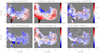 |
Fig. 15 Maps of the kinematic properties. Top: centroid velocity (CV). Bottom: velocity dispersion (FWHM). The two first columns show the kinematic property for the inner and outer (foreground or background) layers, while the last column shows either the subtraction or the ratio of the inner physical property divided by the outer one. |
5.5 Physical state
Figure 16 shows the spatial variations of the gas physical conditions (kinetic temperature, volume density, and thermal pressure) for the inner and outer layers. It also shows the maps of the ratio of these three parameters in the inner and outer layers.
As expected, the kinetic temperature of the inner layer is almost always lower than that of the outer layer when AV ≥ 7 mag, and the inner layer has a higher volume density than the outer layer for the same LoSs. However, while the temperatures of the inner and outer layers are different by a factor of a few, the volume density of the inner layer increases by more than one order of magnitude toward the two dense cores. This explains why the map of the ratio of the thermal pressures (Pther = n Tkin) in the inner to outer layers resembles more that of the ratios of the volume densities than that of the ratio of kinetic temperatures.
The inner layer of the eastern dense core is colder than that of the western dense core. This is consistent with the fact that CO depletion onto dust grains is much more prominent toward the eastern dense core LoS. The western dense core lies close to an embedded Young Stellar Object (YSO) (Position I). The presence of this YSO could provide an additional source of heating of the inner layer around this position.
The outer layer shows a decreasing gradient of both the volume density and thermal pressure from west to east. In particular, toward the eastern dense core, the thermal pressure of the inner layer is 1.9 times lower than that of the same layer toward the western dense core. Such a gradient could be related to the compression associated with the irradiation of the cloud by the σ Ori star (see Ward-Thompson et al. 2006), creating a PDR on the east side.
The volume density and thermal pressure maps show several outliers. For instance, regions around the LoSs E and G have a high volume density and thus thermal pressure. These two LoSs belong to transition zones between the dense cores and their surroundings.
6 Discussion: Comparison of the estimated mean abundances with the model proposed by Tafalla et al. (2021)
To model the line emission toward the Perseus, California, and Orion A molecular clouds, Tafalla et al. (2021, 2023) introduce and apply a model of the abundance of molecular species as a function of the H2 column density (a summary is given in Appendix G). We refer to this model as the TUH one from this point on. The left panel of Fig. 17 overlays TUH model onto the joint distributions of the estimated volume density of the inner layer as a function of the H2 column density. The two models are consistent for log(N(H2)/cm−2) > 21.8, but they show differences of about a factor of two for lower column densities.
The middle and right panels of Fig. 17 overlay the TUH model onto the joint distributions of the estimated mean abundance of 12CO and HCO+ versus H2 column density toward the Horsehead nebula. These joint distributions are identical to these displayed in Fig. 14, except that the molecular visual extinctions were scaled to the H2 column density using Eq. (33). For an easier comparison, we also show the fits listed in Table 6.
The 12CO mean abundance profile that we derive toward the Horsehead nebula is different from TUH one. Our power-law fit reaches its maximum for log(N(H2)/cm−2) = 21.8, while TUH model starts to decline at log(N(H2)/cm−2) ~ 21.3. Moreover, the maximum abundance of 12CO is two to three times higher than that predicted by the TUH model.
In contrast, the agreement between our estimated HCO+ mean abundance profile and TUH model is good for 21.4 < log(N(H2)/cm−2) < 22.2. Both profiles show a slow decrease as N(H2) increases. Above log(N(H2)/cm−2) = 22.2, our estimation yields a steeper fall of the HCO+ abundance than TUH model, but TUH model still lies within our fit confidence interval.
For both species, TUH model predicts a sharp drop of the abundance below log(N(H2)/cm−2) ≲ 21.3 or AV = 2 mag, resulting from the molecule photodissociation. The Horsehead nebula contains few LoSs in this AV regime at the very outskirts of the pillar. It is thus difficult to draw a robust conclusion for this regime.
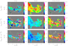 |
Fig. 16 Maps of the gas physical conditions. From top to bottom: kinetic temperature, volume density, and thermal pressure. The first two columns display the values for the inner and outer (foreground or background) layers, while the last column shows their ratio. |
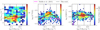 |
Fig. 17 Comparison between the sandwich and TUH models. Left: volume density of the inner layer |

7 Conclusions
In this paper, we have proposed a multilayer model that allows us 1) to fit the low−J lines of different species toward a heterogeneous LoS and 2) to recover information about the chemical abundances, the kinematics, and the physical state (kinetic temperature and volume density) of the gas at different depths along the LoS. To do this, we introduced a fast and efficient maximum likelihood estimator that simultaneously fits all the lines available for each pixel independently.
We also took special care in selecting adequate physical and chemical assumptions in order to avoid biasing the results. Following the recommendations of Roueff et al. (2024), we not only searched for small and unbiased fit residuals but also coherent physical and chemical results. More precisely, in addition to fixing the LoS geometry to three layers (similar to a core surrounded by an envelope), we approximated a centroid velocity gradient along the LoS by allowing the layers to have different velocities in order to be able to reproduce the observed line asymmetries. We also proposed a varying chemistry along the LoS in order to take into account the different processes (e.g., fractionation or molecular freeze-out) at play when the gas is more or less exposed to far UV or more or less dense and cold. While we assumed that the relative abundances 12CO/13CO, C18O/13CO, and H13CO+/HCO+ scale with the elemental abundances of the corresponding carbon and oxygen isotopes in the inner dense layer, we fit the column densities of 12CO,13 CO, C18O, and HCO+ in the outer translucent layer, and we deduced the column density of H13CO+ with the constraint N(H13CO+)/N (13CO) = N (HCO+)/N (12CO).
We used this model to fit the (1 − 0) and (2 − 1) lines of the CO and HCO+ isotopologues toward the translucent, filamentary, and dense core LoSs in the Horsehead pillar. Our main astrophysical findings are as follows:
A precise modeling of the chemistry and physics toward filaments and dense cores requires a heterogeneous model composed of at least an inner dense layer surrounded by two outer translucent layers.
The proposed model succeeds in reproducing integrated intensities within 20% for all lines. The associated bias is small for the 13CO and C18O lines.
We quantitatively confirm that the different lines of the CO and HCO+ isotopologues are sensitive to different depths along the LoS: The emission from the 12CO (1 − 0) line is dominated by the foreground layer (85%). The integrated intensity of the 13CO (1 − 0) and (2 − 1) lines comes from all three layers at approximately the same share. The inner layer has the largest contribution to the total integrated line intensity of the C18O (1 − 0) and (2 − 1) lines, about 60%. The emission from the HCO+ and H13CO+ (1 − 0) lines is dominated by the outer layers (foreground and background), but the inner layer also contributes significantly. Moreover, the emission from the HCO+ and H13CO+ (1 − 0) lines is sub-thermalized with an excitation temperature lower than 10 K.
Deduced chemical properties clearly show 1) the depletion of CO isotopologues toward the dense core LoSs and 2) the increase of the 12CO and HCO+ column density as a function of AV or G0/AV in the warm translucent LoSs. The basic abundances of 12CO, 13CO, and C18O defined in Eq. (24) are reached at visual extinction between 3 and 7 mag, respectively. The typical mean abundance of HCO+ with respect to H2 is ~1.3 × 10⁻⁹, which is about two times lower than the usual value in diffuse clouds (Gerin et al. 2019). The estimated column density ratio N(13CO)/N(C18O) in the envelope increases with decreasing visual extinction and reaches 25 in the pillar outskirts.
In addition to confirming the general rotation of the Horsehead pillar around its axis, we found the signature of accreting motions of the foreground layer onto the inner denser gas.
While the inferred Tkin of the envelope varies from 25 to 40 K, that of the inner layer drops to ~15 K in the western dense core. The estimated
 in the inner layer is ~3 × 104 cm−3 toward the filament, and it increases by a factor of ten toward dense cores. The thermal pressure of the outer layer shows a decreasing east-west gradient.
Except for the abundance ratios in the inner layer that were fixed to ease the estimation in the dense core LoSs, the parameters were estimated from the data with confidence intervals. It will be useful to analyze other datasets in order to check whether the used physical and chemical hypotheses depend on the considered region. If they indeed depend on the physical gas conditions or region, trying to process large maps would imply automatically selecting the most suitable assumptions for a given LoS. This would probably require some insight into the dominant chemical processes as a function of the typical volume density and kinetic temperature. Processing large maps will also require dealing with spectra that present multiple velocity components.
Acknowledgements
We thank the referee for useful comments that helped us improve the manuscript. This work is based on observations carried out under project numbers 019-13, 022-14, 145-14, 122-15, 018-16, and finally the large program number 124-16 with the IRAM 30m telescope. IRAM is supported by INSU/CNRS (France), MPG (Germany) and IGN (Spain). This work received support from the French Agence Nationale de la Recherche through the DAO- ISM grant ANR-21-CE31-0010, and from the Programme National “Physique et Chimie du Milieu Interstellaire” (PCMI) of CNRS/INSU with INC/INP, cofunded by CEA and CNES. M.G.S.M. and J.R.G. thank the Spanish MICINN for funding support under grant PID2019-106110GB-I00. M.G.S.M acknowledges support from the NSF under grant CAREER 2142300. Part of the research was carried out at the Jet Propulsion Laboratory, California Institute of Technology, under a contract with the National Aeronautics and Space Administration (80NM0018D0004). D.C.L. acknowledges financial support from the National Aeronautics and Space Administration (NASA) Astrophysics Data Analysis Program (ADAP).
Appendix A Corrections to the measured visible extinction
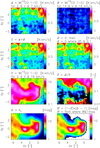 |
Fig. A.1 Steps to correct the visual extinction for 1) the line integrated emission that arises outside of the [7, 14 km s–1], and 2) the contribution from atomic hydrogen. |
The visible extinction estimated from the dust spectral energy distribution is a measure of all hydrogen atoms present along each line of sight. In order to deduce the amount of molecular hydrogen associated to the modeled lines, we thus needed to correct it for two effects that are illustrated in Fig. A.1.
First, Pety et al. (2017) show that the southwestern edge of the Orion B GMC has on average two velocity components: the brightest one centered around 10.5 km s−1 and a fainter one centered around 5 km s–1. Each of them has a typical FWHM of 4 km s–1. The model fitted in this paper still has limitations to be able to fit multiple velocity components. We thus restricted the studied velocity interval around the bright component, namely, between 7 and 14 km s–1. We used the method presented in Einig et al. (2023) to define a position-position-velocity mask of LoS containing some signal on the 13CO(1 – 0) line. We choose this line as the best compromise between optical depth and S/N. We estimated that the relevant velocity interval is [2,16] km s–1. It is thus obvious that part of the estimated visual extinction is associated with line emission between [2,7] km s–1 and [14,16] km s–1. We thus computed the 13CO(1 – 0) integrated intensity inside these two intervals. This integrated intensity map has negative values in regions where the S/N is low. An estimation based on the negative intensity values leads us to conclude that we can only trust the integrated intensity inside the above velocity intervals when it is larger than 0.1 K km s−1. We thus set the integrated intensity to 0 when it is lower than 0.1 Kkm s–1. We then computed the intensity integrated inside [2, 16] km s–1 , and the contribution of the [2, 7] km s−1 and [14, 16] km s–1 velocity intervals to the 13CO(1 – 0) intensity integrated inside [2, 16] km s–1. This allowed us to compute the fraction of the 13CO(1 – 0) integrated intensity coming from the [7, 14] km s–1 velocity interval.
Second, part of the hydrogen may still be in atomic form. Looking at the HI emission toward the Orion B GMC, Pety et al. (2017) estimate that about 1 mag of visual extinction is coming from atomic hydrogen. We thus subtracted 1 mag to the total dust extinction, and we applied the previously computed fraction to this dust extinction corrected for the atomic contribution. This gives the amount of visual extinction coming from molecular gas in the [7,14] km s−1 velocity interval. As the low AV part is still uncertain, we additionally nullified all the LoSs whose visual extinction associated with molecular gas is lower than 1 mag. In this study, we use this “molecular” visual extinction.
Appendix B Radiative transfer equation for a M-layer cloud
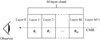 |
Fig. B.1 Sketch of a M-layer model of a line of sight. Each slab has homogeneous physical and chemical conditions (characterized by the parameter vectors θi, for 1 ≤ i ≤ M). The emission from the CMB (layer M + 1) happens at infinity, and it is assumed homogeneous and isotropic. |
Let a M-layer cloud model of the LoS as depicted in B.1. A simple generalization of the computation for a sandwich model (including the ON-OFF calibration procedure) yields
![Mathematical equation: $\matrix{ {{s_M} = \sum\limits_{i = 1}^M {J\left( {{T_{ex,i}}} \right)\left[ {1 - \exp \left( { - {{\rm{\Psi }}_i}} \right)} \right]\exp \left( { - \sum\limits_{j = 1}^{i - 1} {{{\rm{\Psi }}_j}} } \right)} } \cr { - J\left( {{T_{CMB}}} \right)\left[ {1 - \exp \left( { - \sum\limits_{k = 1}^M {{{\rm{\Psi }}_k}} } \right)} \right].} \cr } $](/articles/aa/full_html/2024/12/aa51567-24/aa51567-24-eq94.png)
Assuming that there exist a layer 0 of opacity Ψ0 = 0, we can rewrite this equation as
![Mathematical equation: ${s_M} = \sum\limits_{m = 0}^M {\left[ {J\left( {{T_{ex,m + 1}}} \right) - J\left( {{T_{ex,m}}} \right)} \right]\exp \left( { - \sum\limits_{k = 0}^m {{{\rm{\Psi }}_k}} } \right)} ,$](/articles/aa/full_html/2024/12/aa51567-24/aa51567-24-eq95.png) (B.1)
(B.1)
where we have written J(TCMB) = J(Tex,0) = J(Tex,M+1) only for mathematical convenience (i.e., it is not physically interpretable). This alternate expression simplifies the computation of the Fisher matrix and Cramér-Rao bound.
Indeed, developing Eq. (B.1), we have
![Mathematical equation: $\matrix{ {{s_M} = J\left( {{T_{{\rm{ex,1}}}}} \right)\left[ {1 - \exp \left( { - {{\rm{\Psi }}_1}} \right)} \right]\exp \left( { - {{\rm{\Psi }}_0}} \right)} \hfill \cr {\,\,\,\,\,\,\,\,\,\,\, + J\left( {{T_{{\rm{ex,2}}}}} \right)\left[ {1 - \exp \left( { - {{\rm{\Psi }}_2}} \right)} \right]\exp \left( { - {{\rm{\Psi }}_0} - {{\rm{\Psi }}_1}} \right)} \hfill \cr {\,\,\,\,\,\,\,\,\,\,\, + \cdots } \hfill \cr {\,\,\,\,\,\,\,\,\,\,\, + J\left( {{T_{{\rm{ex,}}M}}} \right)\left[ {1 - \exp \left( { - {{\rm{\Psi }}_M}} \right)} \right]\exp \left( { - \sum\nolimits_{j = 0}^{M - 1} {{{\rm{\Psi }}_j}} } \right)} \hfill \cr {\,\,\,\,\,\,\,\,\,\, - J\left( {{T_{{\rm{CMB}}}}} \right)\left[ {1 - \exp \left( { - \sum\nolimits_{k = 0}^M {{{\rm{\Psi }}_k}} } \right)} \right].} \hfill \cr } $](/articles/aa/full_html/2024/12/aa51567-24/aa51567-24-eq96.png)
Reorganizing the terms yields
 (B.2)
(B.2)
and
 (B.3)
(B.3)
By factorizing each term  for m ⩽ M in Eq. (B.3), we get
![Mathematical equation: $\eqalign{ & {s_M} = \left[ {J\left( {{T_{{\rm{ex}},1}}} \right) - J\left( {{T_{{\rm{ex}},0}}} \right)} \right]\exp \left( { - {\Psi 0}} \right) \cr & \,\,\,\,\,\,\,\,\, + \left[ {J\left( {{T_{{\rm{ex}},2}}} \right) - J\left( {{T_{{\rm{ex}},1}}} \right)} \right]\exp \left( { - {\Psi 0} - {\Psi 1}} \right) \cr & \,\,\,\,\,\,\,\, + \cdots \cr & \,\,\,\,\,\,\, + \left[ {J\left( {{T_{{\rm{ex}},M + 1}}} \right) - J\left( {{T_{{\rm{ex}},M}}} \right)} \right]\exp \left( { - \sum\nolimits_{k = 0}^m {{\Psi k}} } \right). \cr} $](/articles/aa/full_html/2024/12/aa51567-24/aa51567-24-eq100.png)
This form can be rewritten as Eq. (B.1).
Appendix C Negative log-likelihood minimization
One technical challenge of the proposed sandwich model is to define an algorithm that converges within a reasonable amount of time to the parameter vector θ that minimizes the NLL:
 (C.1)
(C.1)
where the sum is performed on all the observed lines xl and the sandwich modeled lines sl (θ), parametrized by the unknown vector θ (see Eq. (1)). The challenge here is that the number of unknowns is much larger than in Roueff et al. (2024) for the same amount of observed information.
Lines of sight are processed independently of each other. The main steps of the minimization of Eq. C.1 are similar to these described in Roueff et al. (2024): An initial estimation of the centroid velocity is followed by a grid search, and finally by a gradient descent.
C.1 Initial estimation of the centroid velocity
We sum the lines of C18O and 13CO to get a bright and approximately thin velocity spectrum. The velocity at which the intensity of the summed spectrum is maximum provides an initial estimation of the centroid velocity CV for all the lines and for both the inner and outer layers.
C.2 Initial optimization with a grid search
We start by searching inside a grid in order to find a good first approximation of the vector θ that minimizes the NLL. We detail here the case of the “improved” model (see Sect. 4.5.3). We need to explore a six- dimentional space {Tkin,  , N(13CO), N(HCO+), FWHM, CV} for the inner layer, and a nine-dimentional space {Tkin,
  , N (12CO), N (13CO), N (C18O), N (HCO+), FWHM, Cν} for the outer layer. Performing an exhaustive grid search is not an option because it would be too time-consuming: Testing ten values per dimension requires 1015 calculations of Eq. C.1. We thus used an iterative stochastic search in a gridded space, that is, a given number of “walkers” randomly explore the 15-dimensional space and converge to their closest local minima. Increasing the number of walkers allows the probability of getting trapped in a local minimum to be decreased, while increasing the number of walker steps is useful to ensure convergence.
To save CPU time, the opacity (τl) and excitation temperature (Tex, l) of each molecular species l are pre-calculated with RADEX on fixed grids. As the sampling of parameter space is identical for the inner and outer layers, only one four-dimentional grid per species needs to be pre-computed. This avoids an excessive load on the RAM memory. More precisely, for each molecular line l, we pre-computed τl and Tex, l on the following regularly sampled grid:
The H2 volume density
 is sampled between 102 and 106.5 cm–3 in logarithmic steps of 0.1 (46 values).
The kinetic temperature Tkin is sampled between 4 and 113 K in logarithmic steps of 0.05 (30 values).
The column density of 13CO is sampled between 1013 and 1018 cm−2 in logarithmic steps of 0.05 (102 values).
The other column densities N(12CO), N(C18O), N(HCO+), N(H13CO+) are sampled on the same grid except that they are shifted by the value fixed by the abundance ratios mentioned in Eq. (24).
The FWHM is sampled linearly between 0.25 and 2 km s–1 in steps of 0.05 km s–1 (36 values).
During the random walk, the column densities are probed under the following constraints. For the inner layer,
 (C.2)
(C.2)
For the outer layer, the constraints are less severe:
 (C.3)
(C.3)
Empirically, we found that the following four-stage algorithm provides a satisfactory stochastic optimization in a reasonable amount of time (less than one minute per pixel on a 2024 laptop). At each stage, we select 10 % of the walkers to save CPU time.
We initialize the centroid velocities of the inner and outer layers to the value estimated in App. C.1, and we fix them to these values during stage 1 and 2. We then randomly draw the θ position of 106 walkers in the remaining 13-dimensional space, and we select the 105 walkers located at positions with the lowest NLL values. Indeed, these walkers are the ones who have the highest chance to be located close to the minimum.
Each selected walker moves in a randomly chosen direction with a randomly chosen step size to explore its vicinity. Its θ position is then updated, if and only if the new position decreases the NLL value. Ten such steps are made during this exploratory stage, and at the end we select the 104 walkers whose position corresponds to the lowest NLL values.
Each selected walker now makes 103 steps. In this stage, the two dimensions of centroid velocities are added to the search space. The size of the step along the centroid velocity axes is set to ±10 m/s. At the end of the this stage, we select the 103 walkers located at positions with the lowest NLL values.
Each of the 103 remaining walkers makes 5000 new steps to finalize the convergence.
Obviously, these settings can be adjusted differently. And this algorithm does not provide any guarantee of convergence. To boost confidence in the estimated θ, one can run the procedure several times to check that the result remains unchanged. However, checking the number of walkers that have converged to the minimum NLL value found already gives a useful indication.
C.3 Final optimization with a gradient descent
The solution provided by the grid search can be refined with a gradient descent algorithm for which the Hessian matrix is replaced by the Fisher matrix. At each iteration i, the vector θ is updated such as
 (C.4)
(C.4)
where IF (θ) is the Fisher Information Matrix computed at θ without considering calibration noise (see Eq. (D.5)), ∇θ – log ℒ is the gradient
 (C.5)
(C.5)
and a ∈ [0, 1] is a parameter to control the convergence speed. To estimate a, we compute ℒ(θ) for a = {0.1, 0.5, 1} and we make a quadratic fit to get an estimation of a that minimizes the NLL in the interval [0.1,1]. The gradient descent algorithm is stopped when the difference of NLL between two consecutive iterations is smaller than 10–6 (our criterion convergence), or when the number of iterations reaches 30 (which is enough for the considered problem). During the gradient descent, the abundance ratios remain unchanged. If one decides to apply the gradient on all the searched column density, the constraint from Eq. C.2 and C.3 would be difficult to satisfy, but more important, the Fisher matrix could become singular.
Appendix D Fisher matrix calculation
We compute the Fisher matrix for the M-layer model described in the previous section rather than to the limiting case of the sandwich model.
D.1 Fisher matrix as a function of gradients 
To compute the Fisher matrix for several observed lines x1, …, xL, we just need to sum the Fisher matrices of the different molecular lines
 (D.1)
(D.1)
This section explains the computations required to yield the Fisher matrix for a single line xl.
As discussed in Sect. 3.6, we consider the case where abundance ratios with respect to 13CO are fixed. The vector of unknowns can be written as
![Mathematical equation: $\theta = \left[ {{\theta _1}, \ldots ,{\theta _M}} \right],$](/articles/aa/full_html/2024/12/aa51567-24/aa51567-24-eq111.png) (D.2)
(D.2)
where each layer of index m is characterized by the vector of physical parameters
![Mathematical equation: ${\theta _m} = \left[ {\log {n_{{{\rm{H}}_2},m}},\log {T_{{\rm{kin}},m}},\log N{{\left( {^{13}{\rm{CO}}} \right)}_m},{\rm{FWH}}{{\rm{M}}_m},{C_{V,m}}} \right].$](/articles/aa/full_html/2024/12/aa51567-24/aa51567-24-eq112.png) (D.3)
(D.3)
The Fisher matrix is therefore of size 5M × 5M.
In their Appendix A.2, Roueff et al. (2024) showed that, when the calibration noise is taken into account (see Eq. (14)), the term i, j of the Fisher matrix can be written as
![Mathematical equation: $\eqalign{ & {\left[ {{I_F}\left( {\theta ;{x_l}} \right)} \right]_{ij}} = \left( {{{\sigma _l^2 + \sigma _{c,l}^4\left( {s_M^T{s_M}} \right)} \over {\sigma _{b,l}^2\sigma _l^2}}} \right)\left( {{{\partial s_M^T} \over {\partial {\theta _i}}}{{\partial {s_M}} \over {\partial {\theta _j}}}} \right) \cr & \,\,\,\,\,\,\,\,\,\,\,\,\,\,\,\,\,\,\,\,\,\,\,\,\,\, + \left( {{{\sigma _{b,l}^2\sigma _{c,l}^4 - \sigma _{c,l}^6\left( {{s^T}s} \right)} \over {\sigma _{b,l}^2\sigma _l^4}} - {{\sigma _{c,l}^2} \over {\sigma _{b,l}^2\sigma _l^2}}} \right)\left( {s_M^T{{\partial {s_M}} \over {\partial {\theta _i}}}} \right)\left( {s_M^T{{\partial {s_M}} \over {\partial {\theta _j}}}} \right), \cr} $](/articles/aa/full_html/2024/12/aa51567-24/aa51567-24-eq113.png) (D.4)
(D.4)
where sM is defined in Eq. (B.1), and  .
.
When the calibration noise is neglected, Eq. (D.4) simplifies into
![Mathematical equation: ${\left[ {{I_F}\left( {\theta ;{x_l}} \right)} \right]_{ij}} = {1 \over {\sigma _{b,l}^2}}\left( {{{\partial s_M^T} \over {\partial {\theta _i}}}{{\partial {s_M}} \over {\partial {\theta _j}}}} \right).$](/articles/aa/full_html/2024/12/aa51567-24/aa51567-24-eq115.png) (D.5)
(D.5)
In both cases, only the gradients  for all unknown parameters θi are needed to complete the computations of the Fisher matrix.
D.2 D.2. Computation of 
We differentiate Eq. (B.1) to obtain for each component θi ∈ θi, and for 1 ≤ i ≤ M
![Mathematical equation: $\eqalign{ & \matrix{ {{{\partial {s_M}} \over {\partial {\theta _i}}} = {{\partial J\left( {{T_{{\rm{ex,}}i}}} \right)} \over {\partial {\theta _i}}}\exp \left( { - \sum\nolimits_{j = 0}^{i - 1} {{{\rm{\Psi }}_j}} } \right)} \hfill \cr {\,\,\,\,\,\,\,\,\,\,\, - {{\partial J\left( {{T_{{\rm{ex}},i}}} \right)} \over {\partial {\theta _i}}}\exp \left( { - \sum\nolimits_{j = 0}^i {{{\rm{\Psi }}_j}} } \right)} \hfill \cr } \cr & \,\,\,\,\,\,\,\,\,\,\, - \sum\nolimits_{m = i}^M {\left[ {J\left( {{T_{ex,m + 1}}} \right) - J\left( {{T_{ex,m}}} \right)} \right]} \exp \left( { - \sum\nolimits_{k = 0}^m {{{\rm{\Psi }}_k}} } \right){{\partial {{\rm{\Psi }}_i}} \over {\partial {\theta _i}}}. \cr} $](/articles/aa/full_html/2024/12/aa51567-24/aa51567-24-eq118.png)
Finally,
![Mathematical equation: $\matrix{ {{{\partial {{\bf{s}}_M}} \over {\partial {\theta _i}}} = } \hfill & {{{\partial J\left( {{T_{{\rm{ex}},i}}} \right)} \over {\partial {\theta _i}}}\left[ {1 - \exp \left( { - {{\rm{\Psi }}_i}} \right)} \right]\exp \left( { - \mathop \sum \limits_{j = 0}^{i - 1} {{\rm{\Psi }}_j}} \right)} \hfill \cr {} \hfill & { + {{\partial {{\rm{\Psi }}_i}} \over {\partial {\theta _i}}}\mathop {\mathop \sum \nolimits^ }\limits_M^{m = i} \left[ {J\left( {{T_{{\rm{ex}},m}}} \right) - J\left( {{T_{{\rm{ex}},m + 1}}} \right)} \right]\exp \left( { - \mathop \sum \limits_{k = 0}^m {{\rm{\Psi }}_k}} \right),} \hfill \cr } $](/articles/aa/full_html/2024/12/aa51567-24/aa51567-24-eq119.png) (D.6)
(D.6)
where the terms  and
and  are expressed in D.2.1 and D.2.2 below.
D.2.1 Computation of 
One has

Then,
![Mathematical equation: ${{\partial J\left( {{T_{ex,i}}} \right)} \over {\partial {\theta _i}}} = \left\{ {\matrix{ 0 \hfill & {{\rm{ if }}\quad {\theta _i} = {C_{V,i}},} \hfill \cr {{{\left( {{{hv} \over {k{T_{{\rm{ex}},i}}}}} \right)}^2}{{\exp \left( {{{hv} \over {k{T_{{\rm{e}},i}}}}} \right)} \over {{{\left[ {\exp \left( {{{hv} \over {k{T_{{\rm{ex}},i}}}}} \right) - 1} \right]}^2}}}{{\partial {T_{{\rm{ex}},i}}} \over {\partial {\theta _i}}}} \hfill & {{\rm{ else}}{\rm{. }}} \hfill \cr } } \right.$](/articles/aa/full_html/2024/12/aa51567-24/aa51567-24-eq124.png) (D.7)
(D.7)
D.2.2 Computation of 
One has  Then,
Then,
![Mathematical equation: ${{\partial {\Psi _i}} \over {\partial {\theta _i}}} = \left\{ {\matrix{ {\left[ {{{\partial {\tau _{\rm{i}}}} \over {\partial {\theta _i}}} + {\tau _{\rm{i}}}{{{{\left( {V - {C_{V,i}}} \right)}^2}} \over {\sigma _{V,i}^3}}} \right]\exp \left( {{{ - {{\left( {V - {C_{V,i}}} \right)}^2}} \over {2\sigma _{V,i}^2}}} \right)} \hfill & {{\rm{ if }}{\theta _i} = {\sigma _{V,i}},} \hfill \cr {{\tau _{\rm{i}}}{{\left( {V - {C_{V,i}}} \right)} \over {\sigma _{V,i}^2}}\exp \left( {{{ - {{\left( {V - {C_{V,i}}} \right)}^2}} \over {2\sigma _{V,i}^2}}} \right)} \hfill & {{\rm{ else if }}{\theta _i} = {C_{V,i}},} \hfill \cr {{{\partial {\tau _{\rm{i}}}} \over {\partial {\theta _i}}}\exp \left( {{{ - {{\left( {V - {C_{V,i}}} \right)}^2}} \over {2\sigma _{V,i}^2}}} \right)} \hfill & {{\rm{ else}}{\rm{. }}} \hfill \cr } } \right.$](/articles/aa/full_html/2024/12/aa51567-24/aa51567-24-eq127.png) (D.8)
(D.8)
We now detail how the terms  and
and  are computed.
For  and
and  are numerically estimated with RADEX by a finite difference technique with a step of 0.001 as it done in Roueff et al. (2024).
For θi = log Tkin, i, one has

Then,
 (D.9)
(D.9)
and
 (D.10)
where  and
and  are numerically estimated with RADEX by a finite difference technique with a step of Tkin,i/1024.
For θi = σV, i, one has

Thus,
 (D.11)
where the terms  and
and  are numerically estimated with RADEX by a finite difference technique with a step of FWHMi /128.
For θi = CV,i, one has

and

D.3 Application to the sandwich model
In the case of the sandwich model, M = 3 and θ1 = θ3. One thus has

where θou and θin are the vector of unknowns of the outer and inner layers respectively.
Appendix E Cramér-Rao lower bounds for derived quantities
E.1 Thermal pressure
Following Roueff et al. (2024), we compute the CRB on the logarithm of the thermal pressure Pther, m for each layer m of the sandwich model as
 (E.1)
(E.1)
where  is the off-diagonal term of the Fisher matrix.
E.2 Centroid velocity difference ∆CV = CV,in – CV,ou
Let CV, in and CV,ou, the centroid velocities of the inner and outer layers, respectively. The CRB on ∆CV = CV,in – CV,ou is
 (E.2)
(E.2)
where CRB(CV, in, CV, ou) is the off-diagonal term of the Fisher matrix.
E.3 Total column density
We derive the logarithm of the total column density of a species X, noted log Ntot (X), from the estimation log Nm (X) with
 (E.3)
(E.3)
This section details how we compute the Cramér-Rao lower bound for log Ntot (X). The formula is generalized for any multilayer model in E.3.1 and we deal with the sandwich model case in E.3.2.
E.3.1 Case of an M-layer cloud
Each layer m of the multilayer model is characterized by a five- parameter vector
 (E.4)
(E.4)
The Fisher matrix dimension is 5M × 5M. As explains by Kay (1997, Sect. 3.8, Eq. 3.30), one can then compute the lower bound on the variance of α = 𝑔(θ) with
 (E.5)
(E.5)
where  is the Jacobian matrix. Thus, for the total column density with Eq. (E.3), one has
  , and
, and
![Mathematical equation: ${{\partial g(\theta )} \over {\partial \theta }} = \left[ {{{\partial g(\theta )} \over {\partial {\theta _1}}} \cdots {{\partial g(\theta )} \over {\partial {\theta _{5M}}}}} \right],$](/articles/aa/full_html/2024/12/aa51567-24/aa51567-24-eq152.png) (E.6)
(E.6)
where
![Mathematical equation: ${{\partial g(\theta )} \over {\partial {\theta _i}}} = \left\{ {\matrix{ {{{1{{\log }^{\left. {\log {N_m}{\rm{X}}} \right)}}} \over {\sum\nolimits_{m = 0}^M 1 {0^{\log {N_m}({\rm{X}})}}}}} \hfill & {{\rm{ if }}{\theta _i} = \log {N_m}({\rm{X}}),\forall m \in {\rm{ [[}}1,M{\rm{ ]]}},} \hfill \cr 0 \hfill & {{\rm{ else}}{\rm{. }}} \hfill \cr } } \right.$](/articles/aa/full_html/2024/12/aa51567-24/aa51567-24-eq153.png) (E.7)
(E.7)
E.3.2 Application to the sandwich model
Applying the result of the previous section leads to
 (E.8)
(E.8)
and
 (E.9)
(E.9)
E.4 FWHMin/FWHMou
We let FWHMin and FWHMou be the FWHM of the inner and the outer layers, respectively. We use Eq. (E.5) to compute the CRB on the FWHM ratio. In this case, g(θ) = FWHMin/FWHMou and
 (E.10)
Appendix F Piecewise power-law fit of Ntot as a function of Au
We aim at fitting power-laws through the total column density as a function AV for different ranges of AV. This means to make a linear regression in the log-log space, that is, fitting
 (F.1)
(F.1)
where x = log(Av), y = log Ntot, and x0 is the center of the log Aν bin and bn is an additive noise drawn from a white Gaussian distribution. Equation (F.1) can be written:
 (F.2)
(F.2)
where y = [y1,…,yN]T, z = [α, β]T, S = [b1,…, bN ]T and
 (F.3)
(F.3)
Moreover, to take into account the uncertainty on log Ntot , we assume that the variance of bn is proportional to the CRB of log Ntot. Thus, B ~ 𝒩(0, λ R) where λ is unknown and R is a diagonal matrix with the CRB of log Ntot . The weighted least square estimator of z is then
 (F.4)
(F.4)
and λ can be estimated with
 (F.5)
(F.5)
and the estimation of the covariance of z is
 (F.6)
(F.6)
For a given x, the estimation of y is
 (F.7)
(F.7)
and its variance is
![Mathematical equation: $\eqalign{ & {\mathop{\rm var}} (\hat y) = {\mathop{\rm var}} (\hat \alpha ){\left( {x - {x_0}} \right)^2} + {\mathop{\rm var}} (\hat \beta ) + 2{\mathop{\rm cov}} (\hat \alpha ,\hat \beta )\left( {x - {x_0}} \right) \cr & {\rm{ where }}{\mathop{\rm var}} (\hat \alpha ) = {[\widehat {\bf{\Gamma }}]_{1,1}}{\mathop{\rm var}} (\hat \beta ) = {[\widehat {\bf{\Gamma }}]_{2,2}}{\mathop{\rm cov}} (\hat \alpha ,\hat \beta ) = {[\widehat {\bf{\Gamma }}]_{1,2}}. \cr} $](/articles/aa/full_html/2024/12/aa51567-24/aa51567-24-eq164.png) (F.8)
(F.8)
Appendix G TUH model in a nutshell
Values of the parameters in the TUH model of the abundance profile as a function of the H2 column density.
For CO and HCO+, (Tafalla et al. 2021) assume that the abundance averaged along the LoS, (X), is defined as
![Mathematical equation: $\langle X\rangle \left[ {N\left( {{{\rm{H}}_2}} \right)} \right] = {X_0} \times {f_{{\rm{out }}}}\left[ {N\left( {{{\rm{H}}_2}} \right)} \right] \times {f_{{\rm{in }}}}\left[ {N\left( {{{\rm{H}}_2}} \right)} \right],$](/articles/aa/full_html/2024/12/aa51567-24/aa51567-24-eq165.png) (G.1)
(G.1)
where X0 is a scaling constant, fout mostly models the photodissociation of the species X by the far UV field in translucent gas, and fin mostly models the molecular freeze-out onto dust grains in cold dense cores. They use the following simple analytic expressions
![Mathematical equation: ${f_{{\rm{out }}}}\left[ {N\left( {{{\rm{H}}_2}} \right)} \right] = \left\{ {\matrix{ {\exp \left[ {6\left( {{A_V} - {A_0}} \right)} \right]} \hfill & {{\rm{ if }}{A_V} \le {A_0},} \hfill \cr 1 \hfill & {{\rm{ if }}{A_V} > {A_0},} \hfill \cr } } \right.$](/articles/aa/full_html/2024/12/aa51567-24/aa51567-24-eq166.png) (G.2)
(G.2)
and
![Mathematical equation: ${f_{{\rm{in}}}}\left[ {N\left( {{{\rm{H}}_2}} \right)} \right] = \exp \left( { - {{{n_{{{\rm{H}}_2}}}} \over {{n_{{\rm{fr}}}}}}} \right),$](/articles/aa/full_html/2024/12/aa51567-24/aa51567-24-eq167.png) (G.3)
(G.3)
where A0 and nfr are the visual extinction and volume densities, which characterize the transition zone for the photodissociation and the molecular freeze-out, respectively. They estimate the volume density with
 (G.4)
(G.4)
Appendix H Supplementary figures
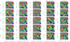 |
Fig. H.3 Joint histograms of the column densities, their abundances, or their ratios as a function of the visual extinction for the studied species. The dashed vertical lines mark the G0/AV values at 1.5, 4.75, and 15 ISRF/ mag. The remainder of the figure layout is identical to Fig. 14. |
References
- Abergel, A., Misselt, K., Gordon, K. D., et al. 2024, A&A, 687, A4 [NASA ADS] [CrossRef] [EDP Sciences] [Google Scholar]
- André, P., Men’shchikov, A., Bontemps, S., et al. 2010, A&A, 518, L102 [NASA ADS] [CrossRef] [EDP Sciences] [Google Scholar]
- Barnes, A. T., Kauffmann, J., Bigiel, F., et al. 2020, MNRAS, 497, 1972 [NASA ADS] [CrossRef] [Google Scholar]
- Bergin, E. A., & Tafalla, M. 2007, ARA&A, 45, 339 [Google Scholar]
- Bron, E., Roueff, E., Gerin, M., et al. 2021, A&A, 645, A28 [NASA ADS] [CrossRef] [EDP Sciences] [Google Scholar]
- Dame, T. M., & Lada, C. J. 2023, ApJ, 944, 197 [NASA ADS] [CrossRef] [Google Scholar]
- Denis-Alpizar, O., Stoecklin, T., Dutrey, A., & Guilloteau, S. 2020, MNRAS, 497, 4276 [Google Scholar]
- Draine, B. T. 2011, Physics of the Interstellar and Intergalactic Medium (Princeton University Press) [Google Scholar]
- Einig, L., Pety, J., Roueff, A., et al. 2023, A&A, 677, A158 [NASA ADS] [CrossRef] [EDP Sciences] [Google Scholar]
- Evans I., Neal J., Kim, K.-T., Wu, J., et al. 2020, ApJ, 894, 103 [NASA ADS] [CrossRef] [Google Scholar]
- Feng, S., Li, D., Caselli, P., et al. 2020, ApJ, 901, 145 [Google Scholar]
- Fuente, A., Garcia-Burillo, S., Usero, A., et al. 2008, A&A, 492, 675 [CrossRef] [EDP Sciences] [Google Scholar]
- Fuente, A., Goicoechea, J. R., Pety, J., et al. 2017, ApJ, 851, L49 [NASA ADS] [CrossRef] [Google Scholar]
- Garthwaite, P. H., Jolliffe, I. T., & Jones, B. 1995, Statistical Inference (London: Prentice Hall Europe) [Google Scholar]
- Gaudel, M., Orkisz, J. H., Gerin, M., et al. 2023, A&A, 670, A59 [NASA ADS] [CrossRef] [EDP Sciences] [Google Scholar]
- Gerin, M., Goicoechea, J. R., Pety, J., & Hily-Blant, P. 2009, A&A, 494, 977 [NASA ADS] [CrossRef] [EDP Sciences] [Google Scholar]
- Gerin, M., Liszt, H., Neufeld, D., et al. 2019, A&A, 622, A26 [NASA ADS] [CrossRef] [EDP Sciences] [Google Scholar]
- Gioumousis, G., & Stevenson, D. P. 1958, J. Chem. Phys., 29, 294 [NASA ADS] [CrossRef] [Google Scholar]
- Goicoechea, J. R., Pety, J., Gerin, M., et al. 2006, A&A, 456, 565 [NASA ADS] [CrossRef] [EDP Sciences] [Google Scholar]
- Goicoechea, J. R., Pety, J., Gerin, M., Hily-Blant, P., & Le Bourlot, J. 2009, A&A, 498, 771 [NASA ADS] [CrossRef] [EDP Sciences] [Google Scholar]
- Goldsmith, P. F., & Kauffmann, J. 2017, ApJ, 841, 25 [Google Scholar]
- Gratier, P., Pety, J., Guzmán, V., et al. 2013, A&A, 557, A101 [CrossRef] [EDP Sciences] [Google Scholar]
- Guzmán, V., Pety, J., Goicoechea, J. R., Gerin, M., & Roueff, E. 2011, A&A, 534, A49 [NASA ADS] [CrossRef] [EDP Sciences] [Google Scholar]
- Guzmán, V., Pety, J., Gratier, P., et al. 2012, A&A, 543, L1 [CrossRef] [EDP Sciences] [Google Scholar]
- Guzmán, V. V., Goicoechea, J. R., Pety, J., et al. 2013, A&A, 560, A73 [Google Scholar]
- Guzmán, V. V., Pety, J., Gratier, P., et al. 2014, Faraday Discuss., 168, 103 [Google Scholar]
- Guzmán, V. V., Pety, J., Goicoechea, J. R., et al. 2015, ApJ, 800, L33 [CrossRef] [Google Scholar]
- Habart, E., Abergel, A., Walmsley, C. M., Teyssier, D., & Pety, J. 2005, A&A, 437, 177 [NASA ADS] [CrossRef] [EDP Sciences] [Google Scholar]
- Hamberg, M., Kashperka, I., Thomas, R. D., et al. 2014, J. Phys. Chem. A, 118, 6034 [CrossRef] [PubMed] [Google Scholar]
- Hernández-Vera, C., Guzmán, V. V., Goicoechea, J. R., et al. 2023, A&A, 677, A152 [NASA ADS] [CrossRef] [EDP Sciences] [Google Scholar]
- Hily-Blant, P., Teyssier, D., Philipp, S., & Güsten, R. 2005, A&A, 440, 909 [NASA ADS] [CrossRef] [EDP Sciences] [Google Scholar]
- Kauffmann, J., Goldsmith, P. F., Melnick, G., et al. 2017, A&A, 605, L5 [NASA ADS] [CrossRef] [EDP Sciences] [Google Scholar]
- Kay, S. M. 1997, Fundamentals of Statistical Signal Processing: Estimation Theory (Prentice Hall) [Google Scholar]
- Kennicutt, R. C., & Evans, N.J. 2012, ARA&A, 50, 531 [NASA ADS] [CrossRef] [Google Scholar]
- Kong, S., Lada, C. J., Lada, E. A., et al. 2015, ApJ, 805, 58 [NASA ADS] [CrossRef] [Google Scholar]
- Lada, C. J., & Lada, E. A. 2003, ARA&A, 41, 57 [Google Scholar]
- Langer, W. D. 1977, ApJ, 212, L39 [NASA ADS] [CrossRef] [Google Scholar]
- Langer, W. D., Graedel, T. E., Frerking, M. A., & Armentrout, P. B. 1984, ApJ, 277, 581 [Google Scholar]
- Liszt, H. S. 2007, A&A, 476, 291 [NASA ADS] [CrossRef] [EDP Sciences] [Google Scholar]
- Lombardi, M., Bouy, H., Alves, J., & Lada, C. J. 2014, A&A, 566, A45 [NASA ADS] [CrossRef] [EDP Sciences] [Google Scholar]
- Mather, J. C., Cheng, E. S., Cottingham, D. A., et al. 1994, ApJ, 420, 439 [Google Scholar]
- Mladenovic, M., & Roueff, E. 2014, A&A, 566, A144 [NASA ADS] [CrossRef] [EDP Sciences] [Google Scholar]
- Myers, P. C., Mardones, D., Tafalla, M., Williams, J. P., & Wilner, D. J. 1996, ApJ, 465, L133 [NASA ADS] [CrossRef] [Google Scholar]
- Ochsendorf, B. B., Cox, N. L. J., Krijt, S., et al. 2014, A&A, 563, A65 [NASA ADS] [CrossRef] [EDP Sciences] [Google Scholar]
- Orkisz, J. H., Peretto, N., Pety, J., et al. 2019, A&A, 624, A113 [NASA ADS] [CrossRef] [EDP Sciences] [Google Scholar]
- Pabst, C. H. M., Goicoechea, J. R., Teyssier, D., et al. 2017, A&A, 606, A29 [NASA ADS] [CrossRef] [EDP Sciences] [Google Scholar]
- Pety, J., Teyssier, D., Fossé, D., et al. 2005, A&A, 435, 885 [NASA ADS] [CrossRef] [EDP Sciences] [Google Scholar]
- Pety, J., Goicoechea, J. R., Hily-Blant, P., Gerin, M., & Teyssier, D. 2007, A&A, 464, L41 [NASA ADS] [CrossRef] [EDP Sciences] [Google Scholar]
- Pety, J., Gratier, P., Guzmán, V., et al. 2012, A&A, 548, A68 [NASA ADS] [CrossRef] [EDP Sciences] [Google Scholar]
- Pety, J., Guzmán, V. V., Orkisz, J. H., et al. 2017, A&A, 599, A98 [NASA ADS] [CrossRef] [EDP Sciences] [Google Scholar]
- Röllig, M., & Ossenkopf, V. 2013, A&A, 550, A56 [NASA ADS] [CrossRef] [EDP Sciences] [Google Scholar]
- Roueff, A., Gerin, M., Gratier, P., et al. 2021, A&A, 645, A26 [NASA ADS] [CrossRef] [EDP Sciences] [Google Scholar]
- Roueff, A., Pety, J., Gerin, M., et al. 2024, A&A, 686, A255 [NASA ADS] [CrossRef] [EDP Sciences] [Google Scholar]
- Santa-Maria, M. G., Goicoechea, J. R., Pety, J., et al. 2023, A&A, 679, A4 [NASA ADS] [CrossRef] [EDP Sciences] [Google Scholar]
- Schinnerer, E., & Leroy, A. K. 2024, arXiv e-prints [arXiv:2403.19843] [Google Scholar]
- Scott, G. B., Fairley, D. A., Freeman, C. G., et al. 1997, J. Chem. Phys., 106, 3982 [NASA ADS] [CrossRef] [Google Scholar]
- Shu, F. H., Adams, F. C., & Lizano, S. 1987, ARA&A, 25, 23 [Google Scholar]
- Tafalla, M., Myers, P. C., Caselli, P., Walmsley, C. M., & Comito, C. 2002, ApJ, 569, 815 [Google Scholar]
- Tafalla, M., Usero, A., & Hacar, A. 2021, A&A, 646, A97 [NASA ADS] [CrossRef] [EDP Sciences] [Google Scholar]
- Tafalla, M., Usero, A., & Hacar, A. 2023, A&A, 679, A112 [NASA ADS] [CrossRef] [EDP Sciences] [Google Scholar]
- van der Tak, F. F. S., Black, J. H., Schöier, F. L., Jansen, D. J., & van Dishoeck, E. F. 2007, A&A, 468, 627 [NASA ADS] [CrossRef] [EDP Sciences] [Google Scholar]
- Visser, R., van Dishoeck, E. F., & Black, J. H. 2009, A&A, 503, 323 [NASA ADS] [CrossRef] [EDP Sciences] [Google Scholar]
- Ward-Thompson, D., Nutter, D., Bontemps, S., Whitworth, A., & Attwood, R. 2006, MNRAS, 369, 1201 [CrossRef] [Google Scholar]
- Yang, B., Stancil, P. C., Balakrishnan, N., & Forrey, R. C. 2010, ApJ, 718, 1062 [Google Scholar]
The basic value of this ratio is 7.94 (see Eq. (24)).
All Tables
References of the rate coefficients used in this article to compute the collisional excitation.
Fitted parameters when assuming that the inner and outer layers have the same or different centroid velocities and velocity dispersions.
Assumptions on column density ratios or relative abundances for the basic and improved sandwich models.
Parameters of the piecewise power-law fits (log(Ntot) = α [log(AV) − log(AV)0] + β) for each studied species.
Values of the parameters in the TUH model of the abundance profile as a function of the H2 column density.
All Figures
|
Fig. 1 Spatial distribution of the peak main beam temperature (Tmb) of the (1 − 0) line of the CO and HCO+ isotopologues as well as of the dust temperature (Tdust), visual extinction (AV), and the ratio of the far UV field over the visual extinction (G0/AV) toward the Horsehead nebula. The used projection is the Azimuthal one rotated by 14° around the center of coordinates RA= 05h40m54.27s, Dec= −02°28′00.00″ in the International Celestial Reference System. Contours of the dust visual extinction at 3, 7, and 16 magnitudes are overlaid on each panel. The crosses and circles show lines of sight that are studied in more detail in this paper (see Table 2 for the corresponding coordinates). |
| In the text | |
|
Fig. 2 Sketch of the multilayer model of a LoS. Top: line of sight decomposed into three layers: the foreground, inner, and background layers. Bottom: inner slab (layer 2) surrounded by two outer slabs that share the same physical and chemical state. Each region has homogeneous physical and chemical conditions (noted θin and θou, respectively). |
| In the text | |
|
Fig. 3 Comparison of five observed spectra (black histograms) and the same ones plus the required amount of noise to saturate their peak S/N to ten (red histograms). The positions of the spectra are marked on Fig. 1 and listed in Table 2. Each row corresponds to a given species and transition, while each column corresponds to a given position. In each panel, the top left and right numbers give the relative weight of a difference of 1 K in any given channel on the fit χ2 value before and after the S/N saturation, respectively. The 12CO (1 − 0) and H13CO+ (1 − 0) lines were observed with a resolution about 5 times coarser than the other lines. When the peak S/N is lower than 10, the red spectrum is hidden under the black one. |
| In the text | |
|
Fig. 4 Comparison of the observed (black) and modeled (red) (1 − 0) line of the 12CO, 13CO, and C18O species for two different LoSs. |
| In the text | |
|
Fig. 5 Comparison of the reconstruction of all integrated line intensities for the best fit obtained with either a homogeneous (in red) or a simple sandwich model (in green). The integrated line intensity or peak temperature are plotted as a function of the visual extinction (AV). More precisely, the integrated line intensities (zero-order moment) or peak temperature are averaged over all the pixels whose visual extinction belongs to the [AV − 0.5, AV + 0.5] mag interval, where AV is plotted on the x-axis of the panels. The lack of values for AV ∈ [23, 24] mag results from the fact that there is no pixel in this range of AV over the studied field of view. In each panel, the top one shows the line integrated intensity or peak intensity, while the bottom one shows the reconstruction relative error in percentage. The colored areas on the relative error panels show the standard deviation over all the pixels that belong to the 1 mag-AV sliding window. The horizontal dashed line indicates a perfect reconstruction. While the simple sandwich model already better fit the data than the homogeneous model, the reconstruction will still be improved by refining the assumptions. |
| In the text | |
|
Fig. 6 Comparison of the data and the fit of the sandwich model when either the centroid velocities of all layers are assumed to be identical (top row) or they can have different values in the inner and outer layers (bottom row). The left and right columns show this comparison for the 13CO (2 − 1) and HCO+ (1 − 0) lines, respectively. These spectra correspond to the LoS B (see Table 2). Data and fitted spectra are shown in black and green lines, respectively. The contributions of the different layers are shown as colored lines: red for the foreground layer (see Eq. (9)), blue for the inner layer (see Eq. (10)), pink for the background layer (see Eq. (11)), and dashed black for the CMB (see Eq. (12)). |
| In the text | |
|
Fig. 7 Comparison of the reconstruction of the 13CO and C18O line integrated intensities for the sandwich model fit obtained with either a fixed relative abundance of [13CO]/[C18O] (in red) or an estimated relative abundance of this ratio (in green). The figure layout is similar to Fig. 5. |
| In the text | |
|
Fig. 8 Comparison of the variations of the NLL as a function of the volume density of the inner layer for the LoS A. We used a sandwich model where N(13CO) and N (C18 O) were fitted, while the column densities of 12CO, HCO+, and H13CO+ were computed assuming fixed abundances relative to 13CO. The top and bottom rows show the NLL variations for two values of N(HCO+)/N(13CO) varying by a factor of 2.0. The left panel shows the NLL variations for the 12CO and 13CO lines, while the right panel show that of the C18O, HCO+, and H13CO+ lines. In both panels, the black plain lines shows the variations of the NLL when fitting all the lines. The top row shows two local minima at similar NLL values while the bottom row only shows one local minimum. The vertical and horizontal black dotted lines intersect at the lowest NLL value, indicated by the red circle, and at the second local minimum that is indicated by the black circle, when it exists. |
| In the text | |
|
Fig. 9 Joint histogram of N(HCO+)/N(12CO) versus N(H13CO+)/N(13CO) in log space for the 3224 chemical models sampling various physical conditions in translucent gas. The red circle shows the ratio derived from the basic abundances listed in Eq. (24). The dashed blue line has a slope of 1.0. |
| In the text | |
|
Fig. 10 Maps of the contributions of the different layers to the line intensity integrated between 8 and 13.5 km s−1. First column: relative error of the model with respect of the data in percentage. Second to fifth columns: contribution of the foreground, inner, background, and CMB layers to the line integrated intensity in percentage of that measured on the data. Each row corresponds to a given line: from top to bottom, 12CO (1 − 0), 13CO (1 − 0) and (2 − 1), C18O (1 − 0) and (2 − 1), HCO+ (1 − 0), and H13CO+ (1 − 0). The percentage on the top center of each panel is the mean±rms value computed over the associated maps. Positive and negative relative errors or contributions are shown in red and blue, respectively. |
| In the text | |
|
Fig. 11 Modeled decomposition of some spectra around the first dense core. Each column corresponds to the spectra for one of the lines of sight listed in Table 2. Each row corresponds to a given line, from top to bottom: 12CO(1 − 0), 13CO(1 − 0) and (2 − 1), C18O(1 − 0) and (2 − 1), HCO+ (1 − 0), and H13CO+ (1 − 0). We show the decomposition of the full spectrum of 12CO (1 − 0) even though we only used its peak intensity during the fit. In each panel, the data and model spectra are shown as the black and green histograms, respectively. The contributions of the foreground, inner, background layers are shown as the plain lines in red, blue, pink, respectively, and the CMB layer is displayed as the dashed black line. |
| In the text | |
|
Fig. 12 Maps of the ratios of the column densities for the outer layer. These ratios have been normalized by the basic values established using the elemental isotopic ratios of carbon and oxygen (see Eq. (24)). By construction N(HCO+)/N(12CO) = N(H13CO+)/N(13CO) (see Sect. 4.5). Contours are drawn at visual extinctions of 3, 7, and 16 mag. |
| In the text | |
|
Fig. 13 Maps of the chemical properties for 12CO, 13CO, C18O, and HCO+, from top to bottom. The three first columns show the column densities for the inner, outer (foreground or background), and total (inner plus twice outer) column densities, while the last column shows the mean abundance, namely, the total column density divided by the H2 column density deduced from the visual extinction. The last column is the ratio of the inner by the outer column density. Contours are drawn at visual extinctions of 3, 7, and 16 mag. |
| In the text | |
|
Fig. 14 Joint histograms of the molecular column densities, abundances, or their ratios as a function of the visual extinction for 12CO, 13CO, C18O, HCO+, and H13CO+, from top to bottom. The three first columns show the column densities for the inner, outer (foreground or background), and total (inner plus twice outer) column densities, while the last column shows the mean abundance, namely, the total column density divided by the H2 column density deduced from the visual extinction. The dashed vertical lines mark the visual extinction at 3, 7, and 16 mag. The red plain lines show the species basic abundance. The black lines show the piecewise power-law fits of the column densities within the AV ranges specified above (see Table 6) and the ±3σ intervals of the fits. These fits can be directly converted to an abundance vs visual extinction relation. |
| In the text | |
|
Fig. 15 Maps of the kinematic properties. Top: centroid velocity (CV). Bottom: velocity dispersion (FWHM). The two first columns show the kinematic property for the inner and outer (foreground or background) layers, while the last column shows either the subtraction or the ratio of the inner physical property divided by the outer one. |
| In the text | |
|
Fig. 16 Maps of the gas physical conditions. From top to bottom: kinetic temperature, volume density, and thermal pressure. The first two columns display the values for the inner and outer (foreground or background) layers, while the last column shows their ratio. |
| In the text | |
|
Fig. 17 Comparison between the sandwich and TUH models. Left: volume density of the inner layer |
| In the text | |
|
Fig. A.1 Steps to correct the visual extinction for 1) the line integrated emission that arises outside of the [7, 14 km s–1], and 2) the contribution from atomic hydrogen. |
| In the text | |
|
Fig. B.1 Sketch of a M-layer model of a line of sight. Each slab has homogeneous physical and chemical conditions (characterized by the parameter vectors θi, for 1 ≤ i ≤ M). The emission from the CMB (layer M + 1) happens at infinity, and it is assumed homogeneous and isotropic. |
| In the text | |
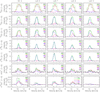 |
Fig. H.1 Same as Fig. 11 but for LoSs around the dense core 2. |
| In the text | |
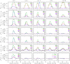 |
Fig. H.2 Same as Fig. 11 but for LoSs at the outskirt of the Horsehead nebula. |
| In the text | |
|
Fig. H.3 Joint histograms of the column densities, their abundances, or their ratios as a function of the visual extinction for the studied species. The dashed vertical lines mark the G0/AV values at 1.5, 4.75, and 15 ISRF/ mag. The remainder of the figure layout is identical to Fig. 14. |
| In the text | |
Current usage metrics show cumulative count of Article Views (full-text article views including HTML views, PDF and ePub downloads, according to the available data) and Abstracts Views on Vision4Press platform.
Data correspond to usage on the plateform after 2015. The current usage metrics is available 48-96 hours after online publication and is updated daily on week days.
Initial download of the metrics may take a while.