| Issue |
A&A
Volume 685, May 2024
|
|
|---|---|---|
| Article Number | A164 | |
| Number of page(s) | 18 | |
| Section | Numerical methods and codes | |
| DOI | https://doi.org/10.1051/0004-6361/202349044 | |
| Published online | 22 May 2024 | |
Fast fitting of spectral lines with Gaussian and hyperfine structure models
Department of Physics,
PO Box 64,
00014
University of Helsinki,
Finland
e-mail: This email address is being protected from spambots. You need JavaScript enabled to view it.
Received:
20
December
2023
Accepted:
5
March
2024
Abstract
Context. The fitting of spectral lines is a common step in the analysis of line observations and simulations. However, the observational noise, the presence of multiple velocity components, and potentially large data sets make it a non-trivial task.
Aims. We present a new computer program Spectrum Iterative Fitter (SPIF) for the fitting of spectra with Gaussians or with hyperfine line profiles. The aim is to show the computational efficiency of the program and to use it to examine the general accuracy of approximating spectra with simple models.
Methods. We describe the implementation of the program. To characterise its performance, we examined spectra with isolated Gaussian components or a hyperfine structure, also using synthetic observations from numerical simulations of interstellar clouds. We examined the search for the globally optimal fit and the accuracy to which single-velocity-component and multi-component fits recover true values for parameters such as line areas, velocity dispersion, and optical depth.
Results. The program is shown to be fast, with fits of single Gaussian components reaching on graphics processing units speeds approaching one million spectra per second. This also makes it feasible to use Monte Carlo simulations or Markov chain Monte Carlo calculations for the error estimation. However, in the case of hyperfine structure lines, degeneracies affect the parameter estimation and can complicate the derivation of the error estimates.
Conclusions. The use of many random initial values makes the fits more robust, both for locating the global χ2 minimum and for the selection of the optimal number of velocity components.
Key words: radiative transfer / methods: numerical / techniques: spectroscopic / ISM: molecules
© The Authors 2024
 Open Access article, published by EDP Sciences, under the terms of the Creative Commons Attribution License (https://creativecommons.org/licenses/by/4.0), which permits unrestricted use, distribution, and reproduction in any medium, provided the original work is properly cited.
This article is published in open access under the Subscribe to Open model. This email address is being protected from spambots. You need JavaScript enabled to view it. to support open access publication.
1 Introduction
Observations of spectral lines are typically analysed by fitting the data with simplified models, and this is also true for the molecular and atomic emission lines observed at radio wavelengths, where the Gaussian approximation is the most common one. The simplest model can thus consist of a single Gaussian that has three free parameters (central velocity, velocity dispersion, and the peak value). The Gaussian model can in principle be justified by the assumption of a Maxwellian velocity distribution of the gas, if the velocity dispersion is dominated by thermal motions. More generally, the central limit theorem suggests that with enough random motions within the beam (e.g. turbulence), the shape of the observed spectrum approaches a Gaussian. However, the observed spectra are rarely precisely Gaussian, and they can show asymmetries (e.g. due to rotation or infall), contain both a narrow and a wide component (e.g. due to outflows or shocks), or contain completely distinct velocity components due to the line-of-sight alignment of separate gas clouds (e.g. large clouds or observations at low Galactic latitudes). The complexity is often addressed by fitting multiple Gaussians, although the physical interpretation of an individual component can be less clear. However, the sum of the fitted components approximates the observed line profile, and such multi-component fits can be used simply as a tool to estimate quantities such as the peak intensities, line areas, and velocity dispersions. Also the column densities are typically estimated based on the fits rather than by direct integration of the relevant quantities over individual channels, for which the signal-to-noise ratio (S/N) is much worse.
Fits to hyperfine spectra follow the same pattern, combining several Gaussians with fixed velocity offsets and usually with fixed relative strengths. The hyperfine fits still use Gaussians to represent the components of the underlying optical depth, but the fits are also directly concerned with the physical parameters of excitation temperature Tex and the total optical depth τ. There is a qualitative difference to the simpler Gaussian fits above, where the fit is an empirical description of the line intensity profile and, in principle, it could even include a sum of positive and negative Gaussians that individually have no physical interpretation. Similar freedom does not exist in hyperfine fits where a single unphysical velocity component can also lead to the end result being unphysical.
Although the fitting of both Gaussian and hyperfine structure models is in principle technically straightforward, some challenges still exist. These are partly computational, caused by the large line surveys and especially numerical simulations that can produce millions of spectra. When visual inspection of all fits is no longer feasible, one needs methods that are both fast and robust. One factor in the robustness is the selection of the initial parameter values for the optimisation of the fitted model. In non-linear least squares problems, and especially when spectra contain multiple components, it is not guaranteed the optimisation would converge to a globally optimal solution. Some optimisation algorithms, such as simulated annealing or genetic algorithms, are more likely to find the global χ1 minimum, but they also tend to be computationally more expensive. The determination of the optimal number of components becomes another important consideration, which may need to take several factors into account, beyond just the formal goodness of the fit.
Pyspeckit (Ginsburg & Mirocha 2011; Ginsburg et al. 2022), SCOUSEPY (Henshaw et al. 2016, 2019), GaussPy (Lindner et al. 2015), GaussPy± (Riener et al. 2019) BTS (Clarke et al. 2018), and MWYDIN (Rigby et al. 2024) are some of the software packages used in the analysis of radio spectral lines. GaussPy is the Python implementation of the autonomous Gaussian decomposition (AGD) algorithm discussed in Lindner et al. (2015) and has been used extensively in the 21-SPONGE survey (Murray et al. 2017, 2018). GaussPy decomposes any spectra that can be modelled using Gaussian functions and utilises a machine learning algorithm to find the appropriate smoothing parameters for the data. Once trained, GaussPy can decompose around 10 000 spectra with Ncpus (number of central processing units, CPUs) in approximately 3/Ncpu hours (Lindner et al. 2015, see Appendix D). Recently, a fully automated package GaussPy+ was designed based on the GaussPy algorithm and a comparative study of these two programs is given in Riener et al. (2019). GaussPy and GaussPy± do not support more complicated spectral decomposition such as a hyperfine structure. Pyspeckit is another CPU parallelised Python-based spectral fitting tool (Ginsburg & Mirocha 2011; Ginsburg et al. 2022), which includes a range of spectral model functions (Gaussian, Lorentzian, and Voight) and ready-to-use model types (NH3, N2H+, HCN, 13CO, and C18O). It has been used recently for example in the ChaMP survey to analyse the hyperfine structure of HCN (Schap et al. 2017). Various other spectral decomposition pipelines, including astroclover (Zeidler et al. 2021) and pyspecnest (Sokolov et al. 2020), also utilise the fitting tools in Pyspeckit. SCOUSEPY (a Python interface of the program SCOUSE written in IDL; Henshaw et al. 2016) uses the cube fitting module of Pyspeckit. Henshaw et al. (2019) provide a brief description of the spectral statistics using SCOUSEPY where they analysed around 30 0000 pixels and, after smoothing, modelled around 130 000 spectra with a 96.4% success (Henshaw et al. 2019). BTS (Clarke et al. 2018) selects the number of fitted components by analysing the first three derivatives of the intensity (versus velocity), once the spectrum has been smoothed to reduce the effect of observational noise. The number of components is selected automatically based on the reduced χ1 values of the alternative fits. Finally, the program MWYDYN (Rigby et al. 2024) is geared towards the automatic fitting of hyperfine spectra with up to three velocity components. The program uses the standard assumptions of a common excitation temperature and full width at half maximum (FWHM) for all hyperfine components, which are also assumed to have Gaussian profiles. The number of components is selected based on Bayesian information criterion (BIC). The code also checks the neighbouring pixels for better fits and uses those iteratively as initial values for alternative fits.
In this paper, we describe a new computer program, Spectral iterative fitter (SPIF). The computational challenges of large sets of spectra are met by using parallelisation and graphics processing units (GPUs) to speed up the fitting. This allows one to address the problem of initial values in a general way, by simply repeating the fits a number of times with different initial values. It also has become possible to estimate the uncertainty of the fitted parameters with Monte Carlo methods, even for spectral cubes consisting of millions of spectra. In addition to describing the implementation and the basic characteristics of SPIF, we analyse synthetic molecular line spectra, including some more realistic examples from numerical cloud simulations. We use the results to characterise the precision to which the basic Gaussian and hyperfine spectrum models are likely to describe the complexity of real observations.
The contents of the paper are the following. In Sect. 2 we describe the implementation of the SPIF program and the spectral models that are being fitted. The calculations behind the synthetic observations are described in Sect. 3. The results are presented in Sect. 4. We examine there the computational performance of SPIF in the case of Gaussian fits (Sect. 4.1.1) and hyperfine fits (Sect. 4.1.2). Section 4.3 examines how well the fitted spectral models are able to describe the spectra from the cloud simulation, and the question of error estimates is studied separately in Sect. 4.4. We discuss the results in Sect. 5 before presenting the conclusions in Sect. 6.
2 Implementation
The SPIF program can be used to fit spectra with one or more Gaussian components or a hyperfine structure. For N Gaussians, the fitted model is TA,
![Mathematical equation: ${\hat T_{A,i}} = \sum\limits_{k = 1}^N {{T_k}\exp \left[ { - 4\ln 2{{\left( {{{{v_i} - {v_k}} \over {\Delta {v_k}}}} \right)}^2}} \right],}$](/articles/aa/full_html/2024/05/aa49044-23/aa49044-23-eq1.png) (1)
(1)
where the free parameters are Tk for the peak value, Δvk for the full width at half maximum (FWHM) of the Gaussian, and for the central velocity. The index k refers to the fitted component, and i represents an individual velocity channel. The solution is found by minimising the χ2 value
 (2)
(2)
where the sum is over M velocity channels. The error estimate δT is assumed to be the same for all channels in a spectrum. We use later also the quantity  (reduced χ2) that is obtained by dividing χ2 with the degree of freedom.
In the case of hyperfine spectra, the optical depth is first calculated as the sum over individual hyperfine components,
![Mathematical equation: ${\tau _i} = \sum\limits_{k = 1} {\tau \times {I_k}\exp \left[ { - 4\ln 2{{\left( {{{{v_i} - v - {v_k}} \over {\Delta {v_k}}}} \right)}^2}} \right],}$](/articles/aa/full_html/2024/05/aa49044-23/aa49044-23-eq4.png) (3)
(3)
where Ik and vk are the relative opacities and velocity offsets of the hyperfine components and v is the radial velocity. The model for the antenna temperatures TA is
![Mathematical equation: $\hat T_{{\rm{A,i}}}^{{\rm{pred}}} = \left[ {J\left( {{T_{{\rm{ex}}}}} \right) - J\left( {{T_{{\rm{bg}}}}} \right)} \right] \times \left( {1 - {e^{ - {\tau _i}}}} \right).$](/articles/aa/full_html/2024/05/aa49044-23/aa49044-23-eq5.png) (4)
(4)
Here J is
 (5)
(5)
Tbg is the assumed temperature of the source background, and ν is the frequency of the transition. The above relation assumes a single velocity component, resulting in four free parameters: the excitation temperature Tex, the velocity (usually defined as the radial velocity of one of the hyperfine components), the FWHM line width, and the optical depth τ.
SPIF consists of a Python host program and a set of kernels, which are compiled programs implemented using OpenCL1 libraries. At the core of the SPIF program are the optimiser kernels. These allow the calculations to be performed either on the host computer (using just the central processing unit CPU) or alternatively on a graphics processing unit (GPU). The latter provides access to massive parallelisation that is well suited for line fitting, when the inputs consist of a large number (preferably thousands) of spectra that can be fitted independently of each other. We have implemented three optimisers, a naive componentwise gradient descent routine, the Nelder-Mead Simplex algorithm, and a conjugate gradient optimiser. Of these, the gradient descent was intended mainly for initial testing but has turned out to be relatively fast for simple problems. The Simplex and the gradient descent method (in spite of its name) use only the χ2 and no gradient information. This also enables the use arbitrary penalty functions2 or to easily extend SPIF with new spectral models. In the case of the conjugate gradient algorithm, the derivatives relative to the parameters of the Gaussian and the hyperfine models are calculated analytically. Calculations are performed by default in single precision. This is typically on GPUs much faster than the use of double precision. On the other hand, the limited precision could cause problems if derivatives (including those associated with the penalty functions or priors) were calculated numerically.
The user provides SPIF with an initialisation file that lists the FITS files with the spectral cubes for the observations and their error estimates. For hyperfine fits, an additional input file is used to specify the frequency of the transition and the relative velocities vi and intensities Ii of the hyperfine components. The initialisation file includes further the description of the fitted model, any potential penalty functions that are used, and the instructions for the initialisation of the optimised parameters. The initial parameters can be constants, calculated based on the spectra (e.g. using the intensity and velocity of the maximum emission or the average velocity of the emission) or they can be read from an external file as separate parameters for each spectrum. The options for initial values are discussed further in Appendix B and also in Sect. 4.2. At the run time, the model specification is added to the OpenCL kernel code, which is compiled on the fly for the actual calculations. This results in a flexible but computationally efficient system. For example, the penalty functions (or priors) can be any arbitrary c-language expressions that depend on the optimised parameters, global constants, or values read from auxiliary files (individual values for each spectrum). In this paper we use only penalty functions of the form
 (6)
(6)
where y refers to a fitted parameter and y0 is a constant threshold value (in this case a lower limit), and δy is a constant that specifies the steepness of the penalty. SPIF also allows the simultaneous fitting of spectra read from two input files, such as different transitions observed towards the same sky position. This then allows for further constraints, such as using the same radial velocity for both spectra in a pair.
SPIF includes different types of iterations, where each spectrum is fitted multiple times. Once the number of fitted components is selected, a fit can be repeated Niter times with perturbed initial parameter values, and the program will return the results from the fit that resulted in the lowest χ2 value. A non-linear least-squares problem (or more generally non-linear optimisation, allowing for arbitrary penalty functions) can have several χ2 minima. Thus, a fit can converge to a local minimum that depends on the initial values chosen for the free parameters. Figure 1 illustrates the potential problem in the case of just two Gaussian components and noise. The fit may pick some noise peak (frames b–d) or, without further constraints, lead to potentially unphysical solutions with negative components (frames c and d). With large enough Niter and large enough variation in the initial values (also defined in the initialisation file), SPIF should be able to find the solution corresponding to the global χ2 minimum, but other constraints may also be needed.
The uncertainty of the fitted model parameters can be estimated with Monte Carlo simulation. In this iteration the observed TA values are perturbed according to their error estimates. This is repeated NMC times, the distribution of the fitted parameter values providing the information of the uncertainties and correlations between the model parameters. The previous iteration types can also be combined. The first iteration (original spectra fitted with Niter random initial values) provides the estimate for the model parameters, and these are then used as the initial values in the fitting of NMC Monte Carlo realisation of the input spectra. However, the fit can be repeated with different initial values even for each of the NMC Monte Carlo realisations. This increases the probability that the fit to each Monte Carlo sample is also the optimal fit for that noise realisation.
SPIF includes some basic Markov chain Monte Carlo routines, which provide an alternative way to calculate error estimates. However, these are less reliable, because the Markov chains may sometimes show poor mixing. This is partly due to the special challenges with the simulated observations examined in this paper, where the peak TA values of noiseless spectra can vary over many orders of magnitude. Therefore, in the following we concentrate mainly on the use of the Monte Carlo error estimates.
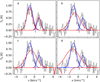 |
Fig. 1 Effect of initial values of the model parameters. The frames show a synthetic spectrum (black histogram) that correspond to two Gaussian peaks (solid blue lines) and white noise. The frames show four potential outcomes, where χ2 minimisation with different initial values has led to different outcomes. The solid red lines show the fitted two components. The fits correspond to local χ2 minima, when no other constraints are used. |
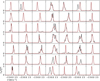 |
Fig. 2 Examples of fits to synthetic spectra from the MHD model (solid black lines) with a single Gaussian component (dashed red lines). The spectra are for C18O (direction x, R = 8) with no added observational noise. The initial values for the intensity and velocity were set based on the peak values in the spectra. The plotted spectra were normalised to a maximum value of one. |
3 Synthetic spectra
We use in the tests synthetic line observations that are based on the magnetohydrodynamic (MHD) simulations of a star-forming cloud presented in Haugbølle et al. (2018) and are similar to the data used in Juvela et al. (2022). The MHD model covers a volume of (4 pc)3 with octree discretisation providing a maximum linear resolution of 100 au or 4.88 × 10⁻⁴ pc. We use a (1.26 pc)3 sub-volume that contains the highest densities. The original MHD cube (with periodic boundary conditions) was rotated to bring the most massive cloud filament to the centre of the model, before selecting the final sub-volume.
The production of synthetic line maps started with the modelling of the dust temperature distribution. The radiation field consists of the external interstellar radiation field (Mathis et al. 1983) and of stellar sources produced as part of the MHD simulation, as described in Juvela et al. (2022). The continuum radiative transfer program SOC (Juvela 2019) was used to solve the dust temperatures for each cell in the model. In the absence of direct information on the gas kinetic temperatures Tkin, the dust temperature was then used as a proxy for Tkin. This is well justified at high densities, n(H2) ≳ 105 cm−3 (Goldsmith 2001; Juvela & Ysard 2011). The modelling of the spectral lines made further use of the density and velocity fields of the MHD simulation. The line maps were produced with the non-LTE radiative transfer program LOC (Juvela 2020). The peak fractional abundances x0 were set to 2 × 10⁻⁶ for 13CO, 2 × 10⁻⁷ for C18O, and 1 × 10⁻¹⁰ for N2H+. We used an additional density scaling (cf. Glover et al. 2010), such that the final density-dependent abundances are
 (7)
(7)
We calculated the 13CO(1−0), C18O(1−0), and N2H+(1−0) spectra, which in the case of N2H+ took into account the full hyperfine structure of the J = 1−0 transition. The background temperature is Tbg = 2.73 K. Further details on the calculations can be found in Juvela et al. (2022).
The radiative transfer calculations resulted in maps for three orthogonal view directions, each with 2576 × 2576 pixels. These corresponds to the highest spatial resolution of the MHD model. However, because of the hierarchical discretisation, the true resolution is lower outside the densest structures. The velocity resolution of the extracted spectra was set to 0.1 km s−1 for the 13CO(1−0) and C18O(1−0) and 0.2 km s−1 for the N2H+ spectra. The total bandwidth is 12 km s−1 for the CO lines and 44.8 km s−1 for N2H+. In the tests we used a series of maps where the number of pixels was further reduced by a factor of R per dimension, once the data were first convolved with a Gaussian beam with FWHM equal to 2R pixels.
4 Results
In this section, we examine fits of Gaussian and hyperfine spectra with the SPIF program. In addition to computational performance (Sect. 4.1), we are interested in how well the Gaussian fits generally reproduce the spectra (Sect. 4.3). This is tested with the help of the data described in Sect. 3. Some characterisation of the synthetic observations can be found in Appendix A. We finish by looking at the error estimation, mainly with the Monte Carlo simulations (Sect. 4.4).
4.1 Computational performance
4.1.1 Gaussian fits
Figure 2 presents examples of the C18O spectra from the MHD cloud model described in Sect. 3, without added observational noise. It shows how the spectra often contain several velocity components, although only up to three distinct peaks among the examples in the figure (cf. Appendix A). The SPIF fits are started using the velocity and intensity of the maximum emission in each spectrum and a fixed FWHM = 1 km s−1 line width. Figure 2 shows examples of the outcome when complex spectra are fitted with a small number of velocity components: the solution may converge to a single peak (not necessarily the strongest one) or the fitted profile can become wide, matching the sum of multiple peaks.
Figure 3 shows the runtimes for one- and two-component Gaussian fits to C18O and 13CO data. In this case, no additional observational noise was added to the spectra obtained from the radiative transfer modelling. The fits were done in using single precision and the R = 1–32 maps, where the total number of spectra ranges from 6480 (R = 32) to 6.6 million (R = 1). The values are for the actual fit and do not include the cost of reading the observations from disk and storing of the results. These are, however, a minor part in the overall runtimes. The timings in Fig. 3 are for the naive gradient descent algorithm. The runtimes of the conjugate gradient algorithm would be similar, while the Simplex method tends to be a few times slower. The fits used all the 120 velocity channels, although significant emission typically covers a smaller fraction of the full bandwidth.
There is a large difference in the speed of the CPU and GPU runs, the latter being faster by almost three orders of magnitude. The leastsq algorithm of the Scipy library3 would reach a speed of some 40 spectra per second, and the CPU speed in Fig. 3 is roughly in line with that, these SPIF run using four CPU cores. Both the CPU and GPU runtimes scale linearly with the number of spectra, and the GPU efficiency drops only for the smallest samples, where the number of spectra falls below the number of physical computing units on the GPU (a top level consumer-grade GPU). There was no significant difference between the C18O and 13CO runtimes.
We next look at the distribution of the χ2 values as a function of noise, the number of fitted Gaussian components, and the number of iterations when fits are repeated with different random initial values. The data correspond to the R = 1 maps of C18O and the combination of all three orthogonal view directions. We remove from the sample spectra where the peak emission remains below 10 mK, leaving about 4.67 million spectra. In the fits with two and three velocity components, we apply additional penalties for negative intensities (Eq. (6) with y = TA, y0 = 0 K, and δy = 0.01 K) and small line widths (y = FWHM, y0 = 0.05 km s−1, and δy = 0.01 km s−1). These reduce the probability for unphysical solutions in the case of multi-component fits, such as spectra decomposed into the sum of arbitrarily large positive and negative components. It also prevents the appearance of very narrow Gaussian components that would fall between velocity channels and could correspondingly have arbitrarily high peak values. Many of our synthetic spectra have intensities that are smaller than the selected values of Sy, resulting in only a small effect from the penalty. A constant Sy is more appropriate for real observations, when all spectra have a similar absolute noise level. The use of penalty functions had no noticeable effect on the runtimes, which are naturally directly proportional to the number of iterations.
Figure 4 shows the  distributions for 1–3 component Gaussian fits with two noise levels and after Niter = 1, 5, and 20 iterations. The noise σ(ΤΑ) was set equal to either 3% or 10% of the maximum value of each spectrum, making the S/N the same for all spectra. The initial values on the first iteration were set according to velocity and intensity of the spectrum maximum, with FWHM = 1 km s−1. On subsequent iterations, the initial value were drawn from a normal distribution with σ equal to 30% around the values on the first iteration. There is a large difference in the normalised χ2 values between the 3% and 10% noise cases, caused by other emission that remains unexplained by the fitted model. With increasing number of retries, the recovered best χ2 values can naturally only decrease. The reduction is noticeable even after five retries, although the improvement is mostly only at 10% level. When the noise is increased to 10% of the peak value, the χ2 values are significantly lower, but the fraction improved fits is not very different from the σ(ΤΑ) = 3% case.
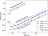 |
Fig. 3 Runtimes of Gaussian and hyperfine fits. Results are shown for Gaussian fits to C18O (red lines) and 13CO (blue lines) spectra and for hyperfine fits to N2H+ spectra (cyan lines). The CPU speeds are slightly below (i.e. faster) than the dotted line for 100 spectra per second. The GPU fits are in the range of 105–106 spectra per second. In the legend, 1G and 2G refer to fits with one or two Gaussian components, respectively. The timings correspond to the x view direction, but the runtimes are nearly identical for the other view directions. |
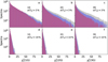 |
Fig. 4 Distributions of |

4.1.2 Hyperfine structure fits
The fits to N2H+ hyperfine spectra were timed using a single velocity component. The fits involved four free parameters and included penalties for small excitation temperatures Tex ≤ Tbg and negative τ values. However, in this case the penalty functions had almost no effect on the results. We examined spectra without added noise and with TA error estimates equal to 3% of the peak value of each spectrum. The initial values for the optimisation were Tex = 5 K, v equal to the mean velocity of the emission, FWHM = 1 km s−1, and optical depth consistent with the assumed Tex value and the maximum antenna temperature of the spectrum. Figure 5 shows examples of fitted spectra.
The runtimes in the analysis of the R = 1–32 maps are included in Fig. 3. The speed on the GPU is about 105 spectra per second, a few times slower than for the single-component Gaussians fits. The increase in the run time is partly due to the larger number of free parameters (although still fewer than for two-component Gaussian fits) and some small overhead from the use of the penalty functions. However, the main cause is simply the larger number of velocity channels, 224 channels compared to the 120 channels in the previous Gaussian fits.
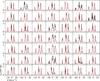 |
Fig. 5 Examples of synthetic N2H+ spectra (solid black lines) and the fitted hyperfine profiles (dashed red lines). The spectra are for direction x, R = 8, and without added observational noise. The y-axis of each frame was scaled independently, and the shown TA axis values apply to the leftmost frames only. |
4.2 Test with synthetic spectra with Gaussian components
In this section, we study simple synthetic spectra with three Gaussian velocity components. These are used to examine the absolute accuracy of the parameter fits as well as the selection of the number of velocity components. The model selection was done using the Akaike information criterion (AIC), which was calculated as AIC = 2k – 2 ln L, where k is the number of free parameters in the model and L is the maximised likelihood4. AIC is but one possible criterion that can be used to choose the optimal number of fitted components, based on the completed fits.
The fitted spectra contain Gaussian components where the peak intensities are 1.0, 0.67, and 0.33 K, central velocities −1.8, 0.6, and 2.3 km s−1, and FWHM values 2.0, 1.5, and 0.5 km s−1, for the three components, respectively. The noise was varied in 50 steps between 1% and 50% of the peak intensity, before adding this normal-distributed noise. We fitted 1000 noise realisations for each noise level to estimate the distribution of the recovered parameters. Figure 6 shows examples of noise realisations, where the three peaks are clearly visible at low noise levels.
The selection of initial values is an important step of model fitting. Apart from reading initial values from external files, SPIF provides a few ways to set the initial values (cf. Sect. 2 and Appendix B). For the first velocity component, we used the intensity and velocity of the spectrum maximum as the initial values. For the second and third component, the intensities were initialised to the same values (i.e. overestimating the true values). The velocities were set to fixed values of 0 and 1 km s−1, respectively, and the FWHM to 1 km s−1. Thus, apart from the intensity and velocity of the first Gaussian, the selected initial values are not particularly close to the true values. This is compensated by repeating the fits with more than twenty times with randomised initial values. The random shifts were generated from N(0, σ), with a standard deviation of σ = 0.2 units (K or km s−1). Thus, the range of initial values does not yet directly cover, for example, the actual radial velocity of the weakest velocity components.
Figure 7 shows the parameters recovered by the 1–3 component Gaussian fits. The single-component fit tries to match all emission, resulting in a mean velocity between the strongest emission components and a large estimated FWHM of ~4 km s−1. With two fitted Gaussians, the first one already gives a good approximation of the strongest emission component while the second fitted Gaussian approximates the sum of the remaining two. When the model uses three Gaussians, these match the three real components accurately up to ~ 10% noise level. Thereafter the intensity of the two weaker features gets systematically overestimated (with S/N <3 for the weakest one), and they move in velocity towards the strongest component.
Using all the velocity channels shown in Fig. 7, the AIC criterion clearly prefers the three-component model for all noise levels below ~10%. Thereafter, as the accuracy of the parameters of the weakest component starts to degrade, also the AIC criterion sometimes prefers the two-component model. However, even at the 50% noise level, the three-component model would still be selected in about half of the cases.
We also checked, how sensitive the AIC criterion is on the inclusion of channels without significant emission. We repeated the analysis after removing 20 channels from both ends of the spectra and thus reducing the total number of channels by some 30%. Although this does change the AIC values, the effect on the model selection is negligible, as shown in Fig. 7. This is not entirely surprising. One can add any number of noisy channels in the AIC calculation, and, as long as the model prediction in these channels is zero, all AIC values increase by the same constant, with no change in their magnitude order. If the model used one component to fit a pure noise feature, that should still get penalised in the AIC comparison. Alternatively, that can be prevented more directly by removing such channels from the analysis altogether, if the channels are known to contain no signal.
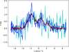 |
Fig. 6 Examples of synthetic spectra with three velocity components. The red, black, blue, and cyan lines correspond to the respective noise levels of 1%, 10%, 30%, and 50% of the peak value in the noiseless spectrum. |
4.3 Tests with synthetic spectra from the MHD simulation
In this section, we examine the precision to which the fitted components reproduce selected properties of the observed spectra. This concerns the differences between complex realistic spectra and the simplified spectral models used in the fits. The accuracy of the error estimates of the fitted parameters is examined later in Sect. 4.4. Here we look only at direct observables, such as the line areas and the velocity dispersion. The more complex question of the connections between the fit parameters and the actual physical source properties (such as the true column density) is mostly beyond the scope of the present paper.
4.3.1 Line area in Gaussian fits
One of the main parameters extracted from Gaussian fits is the line area, which for optically thin lines would also be proportional to the column density (apart from the effects of the line-of-sight Tex variations). It is therefore important to know, how accurately the Gaussian fits are likely to approximate the complex emission from an interstellar cloud, such as approximated by the synthetic observations of the MHD cloud model.
We examined the ratio between the line area provided by Gaussian fits, performed at different noise levels, and the true line areas that were obtained by directly summing the channel values in the original noiseless spectra. Figure 8 shows the results for C18O and 13CO spectra with 1% or 10% of noise (relative to the maximum value in each spectrum). The line areas of the Gaussians are shown for single-component fits (unfilled histograms) and for 1–3 component fits, where the number of components is selected based on AIC. The calculation is in this case done using all channels (a velocity range of 12 km s−1), although the emission often covers less than half of the full bandwidth (cf. Fig. 2). At the σT = 1% noise level, the best Gaussian model recovers the line area relatively accurately, with an rms error of a few percent. If one uses only a single Gaussian, the distribution peaks close to one but, as expected, has a long tail towards lower values, due to the other emission in the spectra. When the noise is increased to 10%, the differences between the different fits decrease. Although the noise increases in the multi-component fits, they remain nearly perfectly unbiased. For the 10% noise level, the Gaussian fits recover the total line area usually with better than ~20% accuracy. However, the accuracy will be worse for complex spectra, and errors larger than 50% are encountered in ~1% of the spectra.
Figure 8 shows no significant differences between C18O and 13CO. This is mainly because the S/N was set equal for every spectrum, and the fraction of optically thick 13CO spectra is still small. In actual observations, the differences between the lines would arise mostly from the different S/N. Our results show no clear difference between the spectrum samples where the peak intensities are  or
or  , in spite of the fact that stronger lines are seen preferentially towards dense regions that are contracting gravitationally and are more likely to have multiple line-of-sight components.
4.3.2 Velocity dispersion from Gaussian fits
We next look at the velocity dispersion deduced from Gaussian fits. Before examining the fits, Fig. 9 shows the overall statistics of the velocity dispersion in the synthetic noiseless spectra. The σv distribution peaks at low values~0.3 km s−1 and moves to lower values for brighter spectra. The values are bound from below by the thermal linewidth (e.g. ~0.05 km s−1 at Tkin = 10K), but the distributions have a long tail that extends even beyond the range shown in Fig. 9 (not visible on the linear scale used in the plot).
Figure 10 compares the standard deviation of the fitted Gaussian components σv(fit) to the actual velocity dispersion σv(true) of the synthetic spectra. The spectra correspond to the R = 2 case and all the three view directions, excluding spectra with Tmax < 1 mK. The comparison is further limited to samples where a single Gaussian component could be expected to give a good representation of the emission. The first sample includes spectra where the single-component fit is preferred based on the AIC criterion. The distribution of the ratio σv(fit)/σv(true) shows two shallow peaks, one around one and another extending down below the ratio of 0.5. This is not surprising, since the spectra often have emission extending over a velocity range several times larger than the individual narrow components. The second sample includes only truly single-peaked spectra, as determined from the noiseless spectra (no multiple local maxima separated by a dip of more than 10%, cf. Appendix A). This narrows the distribution only slightly, as almost all of these spectra also fulfil the AIC criterion for a single component. The sample contains still about one million spectra, some 60% of the spectra in the R = 2 maps. It is only when the calculation of the reference (“true”) velocity dispersion is limited to channels within 1.5σv(fit) of the fitted centre velocity that the σv(fit)/σv(true) distribution peaks more clearly close to the value of one. In that case the fitted Gaussians tend to even slightly overestimate the velocity dispersion of the ±2.5σv(fit) velocity interval. The distribution is still non-Gaussian, with tails extending close to ~20%, even in the case of low noise (σT = 1%). At the higher noise level, the distributions are much wider and the overestimation can reach values above 50%. Although the 13CO spectra are somewhat wider and sometimes optically thick, there is again no clear difference between the C18O and 13CO distributions.
Figure 10 was restricted to cases where the spectra appeared to have just one component, and it showed how difficult it is to estimate the velocity dispersion of a single component. This is even more true if the component needs to be separated from other significant emission features (e.g. Hacar et al. 2018; Lu et al. 2022). Based on Fig. 10, the uncertainty can easily reach 20% in the velocity dispersion and, consequently, would be ~50% in the estimated kinetic energy. If the S/N of the spectrum is sufficient, it may also be better to estimate the velocity dispersion directly from the observed spectrum, instead of relying on Gaussian fits of non-Gaussian profiles.
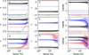 |
Fig. 7 Accuracy of fit parameters in the case of spectra with three Gaussian components. The three rows of frames correspond to the one to three component fits. The solid black, blue, and red lines show the median of the parameter estimates as a function of the noise level, and the shaded areas of the same colour show the inter-quartile ranges. The dotted horizontal lines correspond to the true values. In the frames a, d, and g, the light cyan lines show the fraction of cases where AIC preferred fits with the corresponding number components (i.e. one, two, or three). The dashed dark cyan lines are the same after 40 channels without significant emission were excluded, but these overlap almost perfectly with the previous cyan lines. |
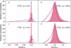 |
Fig. 8 Line areas from Gaussian fits versus the true line area. Results are shown for C18O and 13CO (upper and lower frames, respectively) and for noise levels of σT = 1 % and σT = 10% of the peak value in each spectrum (left and right frames, respectively). The blue histograms contain all spectra with Tmax > 10 mK and the red histograms the strongest spectra with Tmax > 1 K. The unfilled histograms correspond to single-component fits and the filled histograms to one to three component fits, where the number of components was selected based on the AIC criterion. |
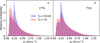 |
Fig. 9 Distribution of the velocity dispersion σν of the synthetic C18O and 13CO spectra without added observational noise. The histograms correspond to spectra with Tmax > 10 mK (blue histograms) and Tmax > 1 K (red histograms). |
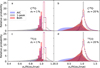 |
Fig. 10 Histograms for the ratio of the velocity dispersion recovered by single-component Gaussian fits (σv(fit)) and the true velocity dispersion of the synthetic spectra (σv(true)). Histograms correspond to spectrum subsets where the best model has only a single velocity component (AIC, based on the AIC criterion), spectra have only a single peak (“1-peak”), and the intersection of these two samples (“both”). The true velocity dispersion was calculated either for the whole spectrum (filled histograms) or only within 2.5σv(fit) around the fitted centre velocity (unfilled histograms). Results are shown for C18O and 13CO (upper and lower frames, respectively) and for noise levels of σT = 1% and σT = 10% (left and right frames, respectively). |
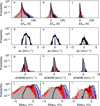 |
Fig. 11 Dispersion of parameter estimates in N2H+ fits of synthetic spectra from the MHD model. From left to right, the frames correspond to synthetic observations in the R = 2, 8, and 32 maps. The filled histograms (in order of increasing width) correspond to noise levels of 1%, 3%, 10%, and 20%. They correspond to the parameter estimates relative to those obtained for spectra without noise (absolute difference on first three rows and logarithm of the ratio in the bottom row). The latter are plotted for reference with solid black lines and shifted to the mean value of zero. |
4.3.3 Parameters of hyperfine structure lines
Figure 11 illustrates the precision of the parameter values obtained from N2H+(1−0) spectra. Unlike in Gaussian fits, the true values of the fitted parameters are not known in a similarly straightforward manner. Therefore, Fig. 11 examines the estimates relative to those obtained in fits of noiseless spectra, which are also used to illustrate the overall range of parameter values. Each histogram in Fig. 11 contains data from all three view directions, excluding spectra with Tmax < 10 mK. When the sample is further reduced to those that are single-peaked in C18O (one velocity component), one is left with 345 340, 24 486, and 2041 spectra for R = 2, 8, and 32, respectively.
The values of velocity and FWHM are recovered very accurately, and even with 20% of added noise, the radial velocity is accuracy to within ~0.1 km s−1. The FWHM is less precise than the velocity itself, and the difference relative to the analysis of noiseless spectra can reach even 2 km s−1. If one had not removed the spectra with multiple velocity components (the larger sample having ~1.49 million, 94 603, and 5869 spectra for R = 2, 8, and 32, respectively), the v and FWHM distribution would be wider by a factor of at least a factor of ~3.
The Tex and τ estimates are affected by strong parameter correlations, and they show much wider scatter (i.e. dependence on the noise level and the noise realisation). In Figs. the τ estimates often vary by more than 100% (Δ log10 τ > 0). With the adopted antenna temperature limit of 10 mK, the sample contains optically thin spectra, for which Tex and τ are degenerate and an individual parameters is almost completely unconstrained. In real observations, many of those spectra would be excluded because of the practical limitations of noise.
Figure 12 separates the previous optical-depth estimates based on the values of the estimated τ, for N2H+ spectra at 3% noise level. The estimates are peaked strongly around ratio one, the optical depth being the same in the analysis of noiseless and noisy spectra. However, there is a fraction of spectra (a factor of 102–103 below the mode of the distributions) where the estimates differ, and the probability for deviations of one order of magnitude are almost as common as smaller changes. Changes larger than a factor of two are observed for 30% of the optically thin spectra (τ = 0.005–0.05), the fraction dropping to 5% for spectra with τ > 1. However, we note than a total optical depth τ = 1 corresponds to an optical depth of only 0.26 for the main hyperfine component. Large changes in the fitted parameters could point to an inaccuracy in the fits. However, Fig. 13 shows ten sample spectra where the ratio of the optical depths derived from spectra without and with noise varies from ~0.1 to 10. In spite of the large differences in τ, all fits are consistent with the data. As the synthetic spectra are the result of a complex line-of-sight integral of emission from different radial velocities and excitation temperatures, they never precisely match the fitted spectral model, and this may also increase the sensitivity to the noise.
Since the uncertainty of Tex and τ values is linked to the low optical depths, we examined separately the spectra that correspond to 10% of the highest column densities in the MHD model. The column densities are obtained directly from the 3D model and thus represent high true optical depths (instead of just high estimated optical depths). The selected spectra also correspond more closely to the regions where N2H+ emission would be in practice observable. In this sample, the average peak temperature is approaching 5 K, and the average optical depth of the main component is ~3. The results are shown in Fig. 14. When compared to the statistics of all the spectra shown Fig. 12 (the middle column with R = 8), the much higher accuracy of the Tex and τ estimates is evident.
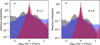 |
Fig. 12 Histograms for the ratio of optical depths derived from fits to noiseless and noisy N2H+ spectra from the MHD model. The colours correspond to optical depth ranges of τ = 0.005–0.05 (grey), τ = 0.05–1 (blue), and τ > 1 (red). The observational noise is 3% of the peak antenna temperature value, and the observations correspond to the R = 2 (frame a) and R = 8 (frame b) spatial resolutions. |
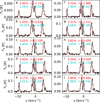 |
Fig. 13 Examples of N2H+ spectra from the MHD model where the ratio of optical depths derived from noiseless and noisy spectra ranges from ~0.1 (frame a) to ~10 (frame j). The black histograms show the observed spectra that contain 3% relative noise. The fits to noiseless and noisy spectra are plotted with dashed red and dotted cyan lines, respectively. The Tex and τ estimates from the fits are listed in the frames in the same colours. |
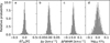 |
Fig. 14 Comparison of N2H+ hyperfine parameters in fits to noiseless spectra and to spectra with 3% relative noise. The sample includes only the lines of sight for 10% of the highest column densities in the MHD model. |
4.4 Error estimates
In SPIF, the main method of error estimation is Monte Carlo simulation. The accuracy of the error estimates can be checked with simulations, However, the simulations are nearly equal to the Monte Carlo estimation itself, with the exception that in the test we can simulate random noise realisations based on true spectra, while the Monte Carlo noise estimation starts with observations that already contain noise.
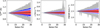 |
Fig. 15 Parameter uncertainties in single-component Gaussian fits to spectra containing one Gaussian. The shaded regions show the error distributions for the estimated parameters as a function of the relative noise 1-30%. The grey, blue, and red colours correspond to [0.01, 99.9], [10, 90], and [25, 75] percentile intervals, respectively. The solid black line shows the median estimates. The solid white lines correspond to the mean 1-σ error estimates (plotted relative to the true values), as obtained from 100 Monte Carlo samples. The white shaded regions correspond to the 1-σ dispersion of the error estimates between spectra at the same noise level. |
4.4.1 Gaussian fits
We look first at simple synthetic spectra that contain one Gaussian component and normal-distributed noise with σ(ΤΑ) ranging from 1% to 30% of the peak value of the spectrum. We examine 322 noise values, each with 322 independent noise realisation, giving slightly more than 100 000 spectra in total.
Figure 15 shows the resulting scatter in the parameter estimates and the error estimates derived for each spectrum with 100 Monte Carlo samples. The small sample of 100 already gives an accurate picture of the 1-σ parameter uncertainties, and even the 1-σ dispersion of the error estimates themselves (white shaded regions in Fig. 15) is relatively small compared to the error estimates. However, if one wants to characterise the tails of the error distribution, beyond the 1-σ level, the computational cost increases rapidly, inversely proportionally to the probability contained in those tails.
We tested next the fitting of two Gaussians that had peak intensities of 1 K and 0.5 K, central velocities of -1 km s-1 and 0.5 km s−1, and FWHM values of 1.5 km s−1 and 1.0 km s−1, respectively. According to Fig. 16, the results are mostly unbiased, although for the weaker component the TA estimates increase and the FWHM estimates decrease with increasing noise. The errors are larger than in the one-component case, and the distribution of radial velocity errors shows stronger tails. For each Monte Carlo sample, the lower of the two radial velocities is always assigned to the first component, which results in some asymmetry in the corresponding error distributions. The error estimates are on average correct, although, compared to Fig. 15, more noisy. In Fig. 16 the 1-σ limits of the error estimates have been smoothed (Gaussian averaging, with FWHM equal to three steps in noise). Nevertheless, they still occasionally show fluctuations exceeding a factor of two (i.e. a large difference between realisations of similar noise). This can be due to pure noise in the error estimates, but is partly true variation: some noise realisations lead to larger uncertainty in the parameter estimates. For these data, AIC prefers the two-component model over one-component model, with very few exceptions at the highest noise levels.
Although the MCMC procedure is less robust than the direct Monte Carlo simulations above, reasonable for MCMC error estimates could be calculates for both the single-component and two-component cases. We reduced the sample of spectra to just 30 realisation at each noise level (a total of 10 304 spectra), mainly to reduce storage requirements (~1GB for each set of MCMC samples) rather than the runtimes. We started the MCMC chains with the maximum likelihood solution and ran a burn-in phase of 1000 steps, during which the step sizes was adjusted to reach ~30% acceptance ratio. We thereafter registered for each spectrum 5000 samples (of the 3 or 6 free parameters), from every 100th MCMC step. Each individual MCMC step is much faster than the full χ1 optimisation, which means that calculations were not more time consuming than the previous runs for the Monte Carlo error estimates. The total runtime of the two-component MCMC calculations was about 13 s (including the host code and the reading and writing of files for the 10 304 spectra), of which some 10 s was spent on actual computations within the OpenCL kernels. This corresponds to an average speed of about 1000 spectra per second. Figure 17 shows the results for one spectrum with 10% relative noise.
Apart from the noise, in the previous examples the spectra matched perfectly the models that were fitted to them. For comparison, we examined the synthetic C18O observations of the MHD model, concentrating on those single-peaked R = 1 spectra where the emission rises above 10 mK. We took a random selection of 10 000 such spectra, added 1–30% of observational noise (at 100 discrete noise levels), registered the maximum likelihood parameter estimates, and estimated their errors based on 100 Monte Carlo samples. The goal was to see if the uncertainties are comparable to those in Fig. 15 or whether other emission in the spectra and deviations from the perfect Gaussian line shapes has a noticeable effect on the errors. In Fig. 18, we rescale the results to a peak value of 1 K, move the central velocity to 0.5 km s−1, and scale the FWHM estimates to 1.5 km s−1 in order to enable more direct comparison to Fig. 15. The errors are larger but this is visible mostly in the tails of the error distribution (in the [0.01,99.9] percentile intervals) and at the higher noise levels (above ~20% relative noise). The line-of-sight confusion of course varies from spectrum to spectrum, and the largest uncertainties exceed even those seen in the two-component fits of Fig. 16.
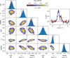 |
Fig. 17 MCMC error estimates for a two-component Gaussian fit. The synthetic spectrum consists of two Gaussian components and white noise with σT = 10% relative to the peak value in the spectrum. The corner plot shows the parameter correlations, where the colours of the 2D histogram correspond to the logarithm of probability (MCMC samples per pixel), as indicated by the colour bar on top. The red crosses correspond to the least-squares solution. The diagonal frames show the histograms for the individual parameters, and the dashed black and red lines correspond to the true values (before observational noise is added) and to the least squares fit, respectively. The frame on the right shows this particular fitted spectrum (black line) and the two components corresponding to the χ2 minimum. |
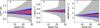 |
Fig. 18 As Fig. 15 but for single-peaked synthetic C18O spectra selected from the MHD cloud model. The white lines show the average ±1-σ Monte Carlo error estimates. |
4.4.2 Hyperfine structure lines
Section 4.3.3 showed that in hyperfine fits the parameters Tex and r are often individually not well constrained. This should be reflected in the error estimates, but it can also complicate the error estimation itself. We examined simulations, where the spectra contained only one velocity component, the emission followed exactly the hyperfine model, and the noise was varied between 1% and 20% of the maximum antenna temperature. The excitation temperature was set to Tex = 9 K and the total optical depth to τ = 0.5. To facilitate comparison with some results obtained with routines from the Scipy library, the SPIF fits included 322 noise levels with 100 spectra each, but only 322 × 5 spectra were used in the comparison to the Scipy fits.
Figure 19 illustrates the parameter degeneracy for one of the spectra at ~3% noise level. After first fitting the four parameters (in this case with the Scipy fmin routine), the velocity and FWHM values were kept constant and the Tex and τ values were varied. The plot shows the resulting plane of χ2 values. The best fits correspond to a narrow valley, where a 1% change in χ2 corresponds to a maximum uncertainty of several degrees in Tex and more than a factor of two in τ, and these just in this one 2D plane. For the total τ = 0.5, all individual hyperfine components are relatively optically thin, and τ thus remains poorly constrained.
Figure 20 shows the distributions of the parameter estimates and the χ2 values for all the 322 × 5 spectra. The SPIF results are compared to fits done with the Scipy library least-squares minimisation routine leastsq and the general optimisation routine fmin with default tolerances, all fits using the same initial values, as indicated in the figure. While the v and FWHM distributions are identical, Tex and τ show differences. The SPIF calculations were done using the fastest option (naive gradient descent and single precision). This results in more sub-structure in the Tex and τ distributions, while also the leastsq and fmin results show some differences. The normalised χ2 values (Fig. 20e) and the corresponding spectrum profiles (not shown) are nevertheless almost identical. If the SPIF runs were carried out using the Simplex method or if the fits were repeated a few times with different initial values, the resulting parameter distributions of SPIF would be close to that of the fmin runs.
While the results of the three routines are not significantly different, the different clustering of the results clearly has the potential to bias the Monte Carlo error estimates. If the τ values were even smaller, the optimisation could stop close to the initial values, leading to severe underestimation of the uncertainty. The use of randomised initial values could again help to obtain more realistic error estimates, even when individual fits showed some dependence on the initial values. Figure 21 shows the distributions of the best-fit parameters (322 noise levels with 100 noise realisation each) and the error estimates from 100 Monte Carlo samples per spectrum. For each Monte Carlo sample, the fit was repeated ten times with initial values sampled from normal distribution with 30% dispersion around the best-fit values. The error estimates are accurate for v and FWHM, and they are of the correct magnitude also for Tex and τ. The procedure has the added benefit of also partly addressing the potential problem of multiple local minima. The Monte Carlo method is still in relative terms more time-consuming, and in this case (32 200 spectra and 100 × 10 separate fits for each), the calculations took some 2.5 min of wall-clock time.
The low optical depth of the above example highlighted the potential problems that parameter degeneracy might cause in error estimation. Similar to Fig. 14, we tested a higher optical depth also in the case of simple single-component synthetic spectra. The results are shown in Fig. 22. The fits correspond to the same 1-20% noise range as in Fig. 20, and the only difference is the higher optical depth, τ = 10 compared to τ = 0.5. This results in better than 1 K accuracy for Tex, while the fractional error in the optical depth can still amount to some tens of per cent at the higher noise levels.
 |
Fig. 19 Example of hyperfine fits with degeneracy between the Tex and τ parameters. The upper frame shows χ2 values over a (Tex, τ) plane, with the χ2 minimum at the centre of the image (the white cross). The white and cyan contours correspond to a 1% and 40% increase over the minimum χ2. The bottom frame shows the spectrum (black line), the original model (spectrum without noise; red line), and the spectrum corresponding to the cyan cross in frame a (dashed cyan line). |
 |
Fig. 20 Comparison of parameter estimates from hyperfine fits with SPIF (red histograms; calculations in single precision) and with Scipy optimisation (blue histograms). The histograms are based on synthetic observations with a single velocity component and a relative noise that was varied between 1% and 20% of the peak value in the spectrum. The vertical dashed lines indicate the true values and the initial values used in the optimisation. The bottom frame shows the normalised χ2 values for each of the fitted spectra. |
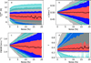 |
Fig. 21 Distribution of best-fit parameters and their error estimates in the case of synthetic N2H+ spectra from the cloud simulation. The sample consists of 100 spectra for each of the 322 noise levels. The black lines show the median parameter estimates, and the shaded red, blue, and grey areas correspond to the [20, 75], [10, 90], and [0.1, 99,9] percentiles of the parameter estimates, respectively. The median Monte Carlo error estimates are shown with solid white curves, and the 1-σ variation of the error estimates (between spectra at the same noise level) with cyan shaded regions. The error estimates are plotted symmetrically relative to the true parameter values. |
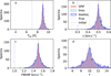 |
Fig. 22 Comparison of parameter estimates from hyperfine fits with SPIF and with Scipy libraries. The figure is similar to Fig. 20 but for spectra with the higher total optical depth of τ = 10. |
5 Discussion
We have presented a new, GPU-accelerated SPIF program for spectral line fitting. Its main characteristic is a relatively good computational performance, which allows the use of repeated fits with random initial values, in order to increase the chances of finding the globally optimal fit. Error estimation with Monte Carlo or MCMC methods is also feasible, even for maps containing thousands of spectra. The performance of the program and some general properties of spectral fits were investigated using synthetic observations.
5.1 Performance of the SPIF program
We were able to fit 105–106 spectra per second with Gaussian models (Fig. 3). However, these numbers depend on many factors, such as the number of velocity channels, the hardware used, the selected initial parameter values, and the number of fitted velocity components. In Fig. 3, the spectra had only 120 channels, the optimisation was done with the fastest option in SPIF and a powerful GPU cards. The more accurate Simplex optimiser was slower by a factor of a few, but still processing ~ 105 spectra per second. The use of penalty functions had only a minor effect on the run times. The third optimiser, the conjugate gradient method, is equally fast, but can be used only when analytical derivatives are provided (including those of the penalty functions).
5.2 Importance of initial values
The tests highlighted the importance of good initial values. Figure 1 showed examples of how a fit can fail by converging to a wrong local minimum, even when spectra contain only two perfect Gaussian components. The situation is usually more complex, as spectra may contain several non-Gaussian velocity components and extended background components of indefinite shape (cf. Fig. 2). The testing of alternative initial values does not help with the model errors (i.e. the observed emission not being the sum of, for example, a few perfect Gaussians) but will increase the probability of finding the global χ2 minimum for the selected model. This is important in multi-component fits, where there are more possibilities for the individual components to converge towards different spectral features.
In the test of Fig. 4, repeats with random initial values improved fits noticeably (more than 20% reduction in χ2) in about one third of the cases. The fraction increased slightly with the increasing number of fitted components, but showed no consistent dependence on the noise level. The numbers of course depend on the complexity of the observed spectra and also on the way the initial values are selected.
5.3 Model errors
If the observations do not match the assumed model, even a technically optimal fit will result in an unbiased view of the emission. We investigated how well the Gaussian fits represent the emission, the line area and velocity dispersion, in the case of the synthetic observations.
In Fig. 8, the analysis of spectra from the MHD model, there was a tendency to underestimate the line areas with the largest errors exceeding 50%. When spectra contain multiple completely separate velocity components, the fit will of course convert the area of one component. Thus, one needs to both select the correct number of component and be successful in fitting them. By choosing the best of the alternative 1-3 component fits (based on AIC) the results were on average unbiased, and the relative uncertainty of the line area was similar to the relative noise in the observed spectra. This is of course not a general rule, since it also depends on how many channels the spectra span. A higher noise could also cause systematic underestimation, as weaker emission components are lost in the noise. In the case of Fig. 8, no such bias was observed. Line area is also a relatively robust parameter. Even when spectra are skew or contain sub-structure, the fitted Gaussian can still provide an accurate estimate of the line area.
In contrast, velocity dispersion σv, is more sensitive to emission at large velocity offsets, and the fit of a small number of Gaussians is likely to correspond to a much lower velocity dispersion. This may also be desirable, when the study concentrates on a component or a few components, and the rest of the emission is unwanted line-of-sight confusion. In Fig. 10 we examined spectra where a single-component fit seemed to be appropriate. However, the single-component Gaussian fits were biased also for this sample, and the velocity dispersion was sometimes underestimated by more than a factor of two. Such errors are very relevant in studies of the cloud energy balance, resulting in large uncertainty in the kinetic energy,  .
.
5.4 Error estimation
Monte Carlo simulation provides a good way to estimate the formal uncertainty and the correlations between the fitted parameters, even when the model includes priors (such as those entered via penalty functions). The method may be feasible even for large samples of millions of spectra, at least for crude error estimates. The noise of the error estimates themselves increases towards the tails of the error distribution, which are therefore much harder to quantify. Figure 15 showed results for fits of a single Gaussian, using only 100 Monte Carlo samples per spectrum. The plotting of [0.01,99.9] percentile interval was possible only because these corresponded to the average over 322 noise realisations. The 100 samples per spectrum may be enough to quantify the error distribution up to 1 − σ level, but the estimation of the [0.01,99.9] percentile range would require 2–3 orders of magnitude more Monte Carlo samples. For example, with one million spectra, 10 000 Monte Carlo samples per spectrum, and 105 fits per second, the computations would still take more than one full day. The tails of the error distribution (more realistically up to 2–3σ levels) are still of some interest, because they may show asymmetries, probability of large deviations, and other deviations from the normal distribution (e.g. Figs. 15 and 16).
We showed that MCMC is a potential alternative for error estimation. This was true at least in the Gaussian fits, even when using the most straightforward Metropolis algorithm. While Monte Carlo method requires one full optimisation, a single MCMC step needs only the evaluation of the χ2 function, and both methods have similar run times. The only concern is the good mixing of the MCMC chains, especially for models with a larger number of parameters and when parameters exhibit very different dynamical ranges. These may require more complex MCMC algorithms, such as the Robust Adaptive MCMC (Haario et al. 2001) or the Hamiltonian MCMC (Betancourt & Stein 2011). Based on preliminary tests, these are however not competitive in very simple cases (such as fits of 1–2 Gaussian components).
One must also exercise some caution in the use of Monte Carlo and MCMC estimates. In models consisting of two Gaus-sians, the fitted components were rearranged so that they appear in velocity order in each Monte Carlo sample. In MCMC calculations, the chains that follow different velocity components can at any point switch identity and continue to follow a different component, especially when the noise is high. This can render the direct chain-averages meaningless, although this did not seem to be a problem in Fig. 17. One should therefore register MCMC samples of a derived quantity that does not depend on the chain identity, such as the total line area (sum over all components, irrespective their order) or directly the total optical depth calculated for each MCMC step. This would thus also directly provide the error distributions for the derived physical quantity.
Compared to the Gaussian fits, the hyperfine fits to synthetic N2H± spectra were more challenging. All parameters cannot be determined accurately either on the optically thin or the optically thick limit. We analysed some optically thin synthetic spectra that showed strong degeneracy between the Tex and τ parameters (Fig. 13, Fig. 19). The degeneracy affects the fits also in a technical sense, as different fitting routines, tolerances, and initial values may all lead to slightly different results (Fig. 20). The run times were somewhat longer than for the Gaussian models (Fig. 3), but just in relation to the larger number of velocity channels in the N2H+ spectra. If optical depths are large, radiative transfer effects also mean that the observed spectrum does no longer exactly match the fitted model. This is not restricted to non-Gaussian line profiles, as spatial variations in excitation conditions, combined with the different optical depths of the components, can also changes in the hyperfine ratios (e.g. Gonzalez-Alfonso & Cernicharo 1993). If Tex and τ cannot be both determined, one option is to fix one of the parameters to a likely value, or to use priors to further constrain the solution (cf. Appendix A in Ginsburg et al. 2022).
We did not carry out any multi-component hyperfine fits. These are more difficult as optimisation problems and may require further priors to avoid unphysical solutions. As noted in Juvela et al. (2022), already in a two-component model there is the risk that some of the Tex values approaches Tbg, which would have a vanishingly small contribution to the modelled intensities but a potentially arbitrarily large contribution to the estimated column densities. These cases need to be excluded, either by using suitable priors or as part of the selection of the best model. The problem does not appear if the components share the same Tex value, but this is not generally a well justified assumption.
5.5 Selection of the best model
In the spectrum analysis, one critical step is the selection of the best model and especially the correct number of fitted components. This can be decided by analysing the spectral shape prior to fits (e.g. Riener et al. 2019), interactively by visual inspection (e.g. Henshaw et al. 2016), or by comparing the statistics of completed alternative fits. The last option could be based on the reduced χ2 values or the use of AIC (in the present paper and in Clarke et al. 2018) or BIC (Rigby et al. 2024). Sokolov et al. (2020) used the Bayesian analysis, which incorporates user-defined priors into the decision process. There the model selection was then based on the ratio of the Bayesian evidences, the joint probability due to likelihood and priors, marginalised over the parameters.
All statistical criteria have their limitations. The observations do not necessarily follow normal statistics, due to observational imperfections that cause deviations from normal statistics (i.e. noise plus baseline errors) and in particular due to model errors, when the spectra contain emission that cannot be accurately described by the chosen model. The Bayesian approach can be powerful, but may also sometimes bias the results towards our expectations. Furthermore, the statistics (such as the basic χ2) depend on the number of channels that do not contain signal but are still included in the analysis. The probability of spurious features also increases as the number of channels is increased (cf. Appendix A in Riener et al. 2019). On the other hand, the exclusion of all channels that do not have significant emission in an individual spectrum will cause more or less bias, depending on the sensitivity of the observations (Yan et al. 2021). Features that are insignificant in an individual spectrum may be significant at the map level. The information from the larger scales (e.g. averaged spectra with higher S/N) can lead to more robust selection of the relevant channels and the number of fitted velocity components. The inspection of spatially averaged emission is part for example of the SCOUSEPY analysis (Henshaw et al. 2019). In details, the selection of the optimal model is also likely to depend on the goals of the analysis. The determination of line area and velocity dispersion have different requirements. In kinematic analysis, it is preferable to avoid random jumps that would be caused by the number of fitted components changing from spectrum to spectrum. Thus, the number of components may need to be fixed over a certain area and common priors need to be used to ensure consistency of multi-component fits. Such analysis is not directly built into the SPIF program but is still partly enabled by it. One possible scheme is to start by fitting spectra convolved to a lower angular resolution (to increase S/N and the spatial correlations) and use those results as direct priors for the fit at the full resolution.
5.6 Comparison to other tools
A number of tools exist for spectral line fitting, and these may also cover related tasks, such as noise estimation and the selection of the optimal number of velocity components to be fitted. Some tools also make it possible to take into account spatial correlations between spectra.
Pyspeckit has an extensive library of spectral fitting tools including specific models for studying the hyperfine structure. Here, the user can define the region of interest either manually or using the built-in GUI. The initial guesses for decomposing the spectra are input parameters, while the program utilises the neighbouring spectra to get initial assumptions for a more efficient fitting. Pyspeckit supports a range of data types and has inbuilt plotting routines. The versatility of the program helps in easily integrating it into different pipelines. For example, SCOUSEPY is another multi-component spectral fitting tool which uses the interactive fitting routine in Pyspeckit (Henshaw et al. 2019). The program allows to targeting of localised regions compartmentalised into several spatially averaged areas (SAA). The corresponding spectra from these user-defined SAAs are obtained using the framework of Pyspeckit. Compared to Pyspeckit, the SPIF program concentrates more on the fitting step only and does not include, for example, specific routines for multi-transition fitting of hyperfine spectra.
GaussPy is an autonomous Gaussian decomposition (AGD) algorithm. It requires one to first transform the data into a format, where each spectrum has its own independent and dependent spectral arrays. The AGD algorithm uses a smoothed spectrum and its higher-order derivatives to find the local maxima and minima to isolate the signal peaks. Users can define one or two (in the case of two-phase decomposition) parameters, α1 and α1, which are the regularisation parameters for the smoothing. We initially fitted a subset of 162 the spectra with GaussPy using an arbitrary α value. The obtained fitting parameters were used to create synthetic Gaussian spectra with a fixed noise level, to train the AGD algorithm to obtain a more accurate α. As α is a measure of the data smoothness and noise suppression, the fitting routine becomes slightly more complicated for data sets with a wide range of noise or component separation (Appendix C).
Figure 23 shows a comparison between GaussPy and SPIF, when fitting the C18O spectra from the MHD model with σ(T) = 0.05 K observational noise. The number of GaussPy components (Fig. 23a), corresponds to the smoothing parameter α that was obtained from a trained AGD. We fitted the 1612 spectra with GaussPy using nine CPUs in approximately 50 min. Compared to the SPIF results with the AIC criterion5, GaussPy produces many more single-component fits and the resulting fit residuals are higher (Fig. 23c).
We carried out the GaussPy fits initially with an arbitrary α value (approximately equal to the channel width, δv). In this case the fit ignored many of the minor velocity components seen in multi-component spectra. With an α obtained from a trained AGD, the ratio of multi-component spectra has increased. With a larger number of spectra in the training set, the accuracy of the α obtained from the trained AGD might be further improved, especially in the case of multi-component spectra.
Figure 24 shows as an example 7 × 7 spectra that are extracted uniformly over the area shown in Fig. 23. As indicated by the previous figure, the AIC criterion tends to choose a larger number of components, which then also leads to lower χ2 values. In some cases, one would clearly choose fewer components by eye, although it is difficult to judge by mere visual inspection the significance of weak features close to the noise level or small deviations from nearly Gaussian line shapes. In contrast, GaussPy is more conservative regarding the number of components, and some spectra appear to remain underfitted. As mentioned earlier, the “correct” number of components depends on the use case and the goals of the analysis, which may thus also necessitate some fine-tuning of the criteria.
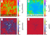 |
Fig. 23 Comparison of GaussPy (left frames) and SPIF (right frames) fits of the C180 spectra of the MHD model. The map resolution is R = 16 and the view direction x. The upper frames show the number of Gaussian components selected by the programs, with the fraction of spectra fitted with one to four components listed within the frames. The lower frames show the corresponding |

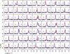 |
Fig. 24 Sample C18O spectra from the MHD model, taken at equidistant positions over the area shown in Fig. 23. The black line shows the synthetic observations with noise equal to σ(T) = 0.05 K. The solid red and dashed blue curves correspond to the SPIF and GaussPy fits, respectively. The number of Gaussian components selected by the methods are indicated in the frames with numbers of the corresponding colour. |
6 Conclusions
We have presented the program SPIF for the fitting of spectral lines. The analysis of its performance and the general tests in fitting synthetic observations with different spectral models have led to the following conclusions:
- 1.
SPIF compares favourably to other fitting routines in computational speed. The use of modern GPUs allows the fitting of simple models (such as 1–2 Gaussians) at a rate approaching 106 spectra per second;
- 2.
SPIF run can include retries, where the fit is repeated with different initial values and the solution of the lowest χ2 value is chosen. This was found to improve the results for a large fraction of the cases, although the typical reduction in χ2 was only at 10% level;
- 3.
The selection of the optimal number of fitted velocity components is not part of the SPIF program. However, as done in the present paper, one can quickly run alternative fits and use afterwards statistical (and other) criteria to choose the most appropriate one;
- 4.
The error estimates derived by Monte Carlo and partially with MCMC method were found to be adequate and also feasible up to samples of tens of thousands of spectra. However, in some cases (such as optically thin lines with hyperfine structure) the error estimates might become dependent on the adopted initial values, and further iterations may be needed to validate the estimates;
- 5.
The above points contribute to the robustness and the relative ease of use of the SPIF program. Thanks to the brute-force approach (the use of a large enough number of retries with random initial values), the default input values will usually result in fits that are nearly optimal.
Acknowledgements
The work was supported by the Research Council of Finland grant 348342.
Appendix A Statistics of the synthetic test spectra
We discuss below some properties of the spectra obtained from MHD cloud simulation. Figure 23 shows the general statistics of the C18O and 13CO spectra. A large fraction of the spectra are multimodal. The histograms in Fig. 23a,e show the number of distinct spectral peaks, where the individual peaks are required to be separated by a dip of at least 10% relative depth, in the spectra containing no observational noise. We exclude individual peaks below 0.1 mK, to avoid potential spurious peaks that could be caused by numerical errors. In the full 2573×2573 pixel maps (R=1), the highest number of peaks is about ten, but these correspond to only a fraction of ~ 10−5 of all spectra. For larger values of R, which also imply convolution with larger beams, multimodal spectra are in relative terms equally common and are rare only due to the smaller total number of spectra. Depending on the assumed observational noise, the synthetic observations should thus often be fitted using multiple velocity components.
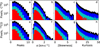 |
Fig. A.1 Statistics for synthetic C18O (upper row) and 13CO (bottom row) spectra. Histograms are plotted for the number of spectral peaks, the line width converted to standard deviation σ, the skewness, and the kurtosis. Each frame contains four histograms that correspond to R=1, 2, 8, and 32, in decreasing order of the histogram height. |
The large absolute values of skewness (Fig. 23c,g) are also due to the presence of multiple velocity components. However, even among the spectra classified as having only a single significant peak, one in four spectra shows at least moderate skewness (|skewness| > 0.5). The fraction tends to be smaller for 13CO spectra and larger R values, but drops below 10% only for stronger spectra above 10 mK. For normal distribution, the skewness and, as calculated in Fig. 23, the kurtosis should both be zero. Based on the central limit theorem, one could have expected that a large beams (larger R) would reduce the kurtosis and the absolute values of skewness. However, as in the case of the number of peaks, the histograms differ mainly just due to the smaller number of spectra. Only the largest kurtosis values are more noticeably reduced as R is increased.
Appendix B Notes on the usage of the SPIF program
We provide here a short overview of the input parameters of SPIF, including the model definition, the use of penalty functions and priors, and the generation of initial values for the fits. A more detailed description can be found in the a pdf document at the project GitHub page6. The input parameters related to the fitted model are provided in a single ini file, and there are also some command-line parameters that are concerned more with the technical details of the calculations
The ini file lists names of the FITS files than contain the spectra, with a separate file for their error estimates. The fitted model is described using pre-defined GAUSS and HFS names, for fits of isolated Gaussian profiles and hyperfine spectra, respectively. The free parameters of the models are listed explicitly as x[0], x[1],etc. One can fit simultaneously spectra from up to two files (e.g. different transitions of the same species), and the use of the same parameter name for both introduces a explicit constraint between the two fits. In the model definition, the term y1 refers to the spectra in the first (and in this case the only) input FITS file, and the term v1 refers to its channel velocities. Thus, a minimal ini-file for fitting a single Gaussians to one set of spectra is
fits1  =  13CO.fits
dfits1 =  13CO_err.fits
y1     =  GAUSS(v1, x[0], x[1], x[2])
prefix =  result
The parameters x[0]-x[2] are the peak temperature, central velocity, and the FWHM value. The fit of spectra from two input files, forced to have the same radial velocity (x[1] ), could be
fits1  =  13CO.fits
dfits1 = 13CO_err.fits
y1     = GAUSS(v1, x[0], x[1], x[2])
fits2  = C18O.fits
dfits2 = C18O_err.fits
y2     = GAUSS(v2, x[3], x[1], x[4])
Initial values for the fit of each spectrum can be read from an external file. However, they can also be set via the ini-file, either to some constant value or as parameters computed from the spectra. The possible computed parameters include the peak intensity (tmax), the velocity of the peak location (vmax), and the FWHM (fwhm) computed over the full spectrum. One also needs to specify, if the calculation is to use the spectra of the first or the optional second spectrum file (y1 vs. y2). As a example, when fitting one set of spectra with two Gaussian components, the ini-file could include lines
y1   =  GAUSS(v1, x[0], x[1], x[2]) ± \
        GAUSS(v1, x[3], x[4], x[5])
init =  y1:tmax   y1:vmax y1:fwhm  \
        y1:tmax/2 y1:vmax±0.5  1.2
The model contains two independent Gaussians and six free parameters, and the initial values are specified in the same order. For the first Gaussian they are directly the values calculated based on the observed spectra, and the second Gaussian uses the same value with some modifications. Only the initial FWHM value of the second Gaussian is set directly to a constant value of 1.2 km s−1.
The ini-file can contain penalty functions and priors. While the penalty function can be an arbitrary c-language expression involving some free parameters, the priors are assumed to be properly normalised probability density functions (e.g. in MCMC calculations). As an example, a penalty for negative values of the free parameter x[0] could be included as
penalty = (x[0]<0.0) ? (-x[0]/0.1) : 0.0
For bias terms, SPIF includes a couple of pre-defined functions, and for example a normal-distributed prior x[1]~ N(2.0, 0.3) can be entered as
bias = NORMAL(x[1]-2.0, 0.3)
The penalty and bias expressions can also refer to values that are read from auxiliary FITS files, one value per spectrum. One possible use case is to set a prior for the fitted velocity based on velocities found in a previous fit of a different line. Further details on the use of external files and other ini-file options can be found on the GitHub page.
Appendix C Synthetic spectra with two Gaussians
Figure C.1 compares the results of the spectral modelling with GaussPy and SPIF for a synthetic two-component spectrum of size 311 x 5. Here, we have introduced a noise level varying from 1% to 33%. We have used GaussPy single-phase fitting for two chosen values of α for two parts of this data cube. For the lower noise levels (< 16%), we use an α approximately close to the channel width, whereas for the higher noise level spectra (> 16%), we fix the α to be around 40 times the channel width. GaussPy is successful in isolating the two components at the lower noise levels. As the noise level increases, it becomes more challenging to fit the multiple components. For chosen values for α1 and α1 even the two-phase decomposition routine failed to capture the multiple components at higher noise levels. While a trained smoothing parameter at different noise levels will better fit the two-component spectra, the widely varying noise levels can still be non-trivial in fixing the degree of smoothness.
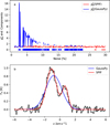 |
Fig. C.1 Fit to spectra containing two Gaussian components and with noise varied from 1% to 30%. The upper frame shows the reduced χ2 values for GaussPy (blue line) and SPIF (red line) fits. The crosses indicate cases where programs have preferred the single-component fit. Some GaussPy fits have failed, and in those cases no χ2 value is plotted. In the case of GaussPy, we modelled the parameter using smoothing parameters α ~ δv for noise ≤ 16% and α ~ 40 × δv for noise > 16%. A fixed smoothing parameter for varying noise levels prevents GaussPy from isolating the multiple components. In the case of SPIF, both one-and two-component fits were performed and the model with the lower AIC values is included in the figure. The lower frame shows one example where GaussPy (blue line) has opted for a single-component fit, resulting in a noticeably higher χ1 value in frame a. |
References
- Betancourt, M., & Stein, L. C. 2011, arXiv e-prints [arXiv:1112.4118] [Google Scholar]
- Cavanaugh, J. E. 1997, Stat. Prob. Lett., 33, 201 [Google Scholar]
- Clarke, S. D., Whitworth, A. P., Spowage, R. L., et al. 2018, MNRAS, 479, 1722 [Google Scholar]
- Ginsburg, A., & Mirocha, J. 2011, Astrophysics Source Code Library [record ascl:1109.001] [Google Scholar]
- Ginsburg, A., Sokolov, V., de Val-Borro, M., et al. 2022, AJ, 163, 291 [NASA ADS] [CrossRef] [Google Scholar]
- Glover, S. C. O., Federrath, C., Mac Low, M. M., & Klessen, R. S. 2010, MNRAS, 404, 2 [Google Scholar]
- Goldsmith, P. F. 2001, ApJ, 557, 736 [Google Scholar]
- Gonzalez-Alfonso, E., & Cernicharo, J. 1993, A&A, 279, 506 [NASA ADS] [Google Scholar]
- Haario, H., Saksman, E., & Tamminen, J. 2001, Bernoulli, 7, 223 [CrossRef] [Google Scholar]
- Hacar, A., Tafalla, M., Forbrich, J., et al. 2018, A&A, 610, A77 [NASA ADS] [CrossRef] [EDP Sciences] [Google Scholar]
- Haugbølle, T., Padoan, P., & Nordlund, Å. 2018, ApJ, 854, 35 [CrossRef] [Google Scholar]
- Henshaw, J. D., Longmore, S. N., Kruijssen, J. M. D., et al. 2016, MNRAS, 457, 2675 [Google Scholar]
- Henshaw, J. D., Ginsburg, A., Haworth, T. J., et al. 2019, MNRAS, 485, 2457 [Google Scholar]
- Juvela, M. 2019, A&A, 622, A79 [NASA ADS] [CrossRef] [EDP Sciences] [Google Scholar]
- Juvela, M. 2020, A&A, 644, A151 [NASA ADS] [CrossRef] [EDP Sciences] [Google Scholar]
- Juvela, M., & Ysard, N. 2011, ApJ, 739, 63 [NASA ADS] [CrossRef] [Google Scholar]
- Juvela, M., Mannfors, E., Liu, T., & Tóth, L. V. 2022, A&A, 666, A74 [NASA ADS] [CrossRef] [EDP Sciences] [Google Scholar]
- Lindner, R. R., Vera-Ciro, C., Murray, C. E., et al. 2015, AJ, 149, 138 [NASA ADS] [CrossRef] [Google Scholar]
- Lu, Z.-J., Pelkonen, V.-M., Juvela, M., et al. 2022, MNRAS, 509, 5589 [Google Scholar]
- Mathis, J. S., Mezger, P. G., & Panagia, N. 1983, A&A, 128, 212 [NASA ADS] [Google Scholar]
- Murray, C. E., Stanimirović, S., Kim, C.-G., et al. 2017, ApJ, 837, 55 [NASA ADS] [CrossRef] [Google Scholar]
- Murray, C. E., Stanimirović, S., Goss, W. M., et al. 2018, ApJS, 238, 14 [NASA ADS] [CrossRef] [Google Scholar]
- Riener, M., Kainulainen, J., Henshaw, J. D., et al. 2019, A&A, 628, A78 [NASA ADS] [CrossRef] [EDP Sciences] [Google Scholar]
- Rigby, A. J., Peretto, N., Anderson, M., et al. 2024, MNRAS, 528, 1172 [NASA ADS] [CrossRef] [Google Scholar]
- Schap, W. J., Barnes, P. J., Ordoñez, A., et al. 2017, MNRAS, 465, 2559 [NASA ADS] [CrossRef] [Google Scholar]
- Sokolov, V., Pineda, J. E., Buchner, J., & Caselli, P. 2020, ApJ, 892, L32 [NASA ADS] [CrossRef] [Google Scholar]
- Yan, Q.-Z., Yang, J., Su, Y., Sun, Y., & Wang, C. 2021, ApJ, 910, 109 [NASA ADS] [CrossRef] [Google Scholar]
- Zeidler, P., Sabbi, E., Nota, A., & McLeod, A. F. 2021, AJ, 161, 140 [NASA ADS] [CrossRef] [Google Scholar]
A penalty function can in principle be any expression containing the optimised parameter. Some examples are included in Appendix B.
We omit the correction for small samples, which would change the expression to  . The corrected formula would set more preference for models with fewer parameters. However, the term is small, ~ 0.1 between our consecutive Gaussian models. To our knowledge, the correction term is also proven only for linear models (Cavanaugh 1997).
We do not consider the use of AIC as part of the SPIF program itself, only as one possible criterion that can be applied based on the alternative fits.
All Figures
|
Fig. 1 Effect of initial values of the model parameters. The frames show a synthetic spectrum (black histogram) that correspond to two Gaussian peaks (solid blue lines) and white noise. The frames show four potential outcomes, where χ2 minimisation with different initial values has led to different outcomes. The solid red lines show the fitted two components. The fits correspond to local χ2 minima, when no other constraints are used. |
| In the text | |
|
Fig. 2 Examples of fits to synthetic spectra from the MHD model (solid black lines) with a single Gaussian component (dashed red lines). The spectra are for C18O (direction x, R = 8) with no added observational noise. The initial values for the intensity and velocity were set based on the peak values in the spectra. The plotted spectra were normalised to a maximum value of one. |
| In the text | |
|
Fig. 3 Runtimes of Gaussian and hyperfine fits. Results are shown for Gaussian fits to C18O (red lines) and 13CO (blue lines) spectra and for hyperfine fits to N2H+ spectra (cyan lines). The CPU speeds are slightly below (i.e. faster) than the dotted line for 100 spectra per second. The GPU fits are in the range of 105–106 spectra per second. In the legend, 1G and 2G refer to fits with one or two Gaussian components, respectively. The timings correspond to the x view direction, but the runtimes are nearly identical for the other view directions. |
| In the text | |
|
Fig. 4 Distributions of |
| In the text | |
|
Fig. 5 Examples of synthetic N2H+ spectra (solid black lines) and the fitted hyperfine profiles (dashed red lines). The spectra are for direction x, R = 8, and without added observational noise. The y-axis of each frame was scaled independently, and the shown TA axis values apply to the leftmost frames only. |
| In the text | |
|
Fig. 6 Examples of synthetic spectra with three velocity components. The red, black, blue, and cyan lines correspond to the respective noise levels of 1%, 10%, 30%, and 50% of the peak value in the noiseless spectrum. |
| In the text | |
|
Fig. 7 Accuracy of fit parameters in the case of spectra with three Gaussian components. The three rows of frames correspond to the one to three component fits. The solid black, blue, and red lines show the median of the parameter estimates as a function of the noise level, and the shaded areas of the same colour show the inter-quartile ranges. The dotted horizontal lines correspond to the true values. In the frames a, d, and g, the light cyan lines show the fraction of cases where AIC preferred fits with the corresponding number components (i.e. one, two, or three). The dashed dark cyan lines are the same after 40 channels without significant emission were excluded, but these overlap almost perfectly with the previous cyan lines. |
| In the text | |
|
Fig. 8 Line areas from Gaussian fits versus the true line area. Results are shown for C18O and 13CO (upper and lower frames, respectively) and for noise levels of σT = 1 % and σT = 10% of the peak value in each spectrum (left and right frames, respectively). The blue histograms contain all spectra with Tmax > 10 mK and the red histograms the strongest spectra with Tmax > 1 K. The unfilled histograms correspond to single-component fits and the filled histograms to one to three component fits, where the number of components was selected based on the AIC criterion. |
| In the text | |
|
Fig. 9 Distribution of the velocity dispersion σν of the synthetic C18O and 13CO spectra without added observational noise. The histograms correspond to spectra with Tmax > 10 mK (blue histograms) and Tmax > 1 K (red histograms). |
| In the text | |
|
Fig. 10 Histograms for the ratio of the velocity dispersion recovered by single-component Gaussian fits (σv(fit)) and the true velocity dispersion of the synthetic spectra (σv(true)). Histograms correspond to spectrum subsets where the best model has only a single velocity component (AIC, based on the AIC criterion), spectra have only a single peak (“1-peak”), and the intersection of these two samples (“both”). The true velocity dispersion was calculated either for the whole spectrum (filled histograms) or only within 2.5σv(fit) around the fitted centre velocity (unfilled histograms). Results are shown for C18O and 13CO (upper and lower frames, respectively) and for noise levels of σT = 1% and σT = 10% (left and right frames, respectively). |
| In the text | |
|
Fig. 11 Dispersion of parameter estimates in N2H+ fits of synthetic spectra from the MHD model. From left to right, the frames correspond to synthetic observations in the R = 2, 8, and 32 maps. The filled histograms (in order of increasing width) correspond to noise levels of 1%, 3%, 10%, and 20%. They correspond to the parameter estimates relative to those obtained for spectra without noise (absolute difference on first three rows and logarithm of the ratio in the bottom row). The latter are plotted for reference with solid black lines and shifted to the mean value of zero. |
| In the text | |
|
Fig. 12 Histograms for the ratio of optical depths derived from fits to noiseless and noisy N2H+ spectra from the MHD model. The colours correspond to optical depth ranges of τ = 0.005–0.05 (grey), τ = 0.05–1 (blue), and τ > 1 (red). The observational noise is 3% of the peak antenna temperature value, and the observations correspond to the R = 2 (frame a) and R = 8 (frame b) spatial resolutions. |
| In the text | |
|
Fig. 13 Examples of N2H+ spectra from the MHD model where the ratio of optical depths derived from noiseless and noisy spectra ranges from ~0.1 (frame a) to ~10 (frame j). The black histograms show the observed spectra that contain 3% relative noise. The fits to noiseless and noisy spectra are plotted with dashed red and dotted cyan lines, respectively. The Tex and τ estimates from the fits are listed in the frames in the same colours. |
| In the text | |
|
Fig. 14 Comparison of N2H+ hyperfine parameters in fits to noiseless spectra and to spectra with 3% relative noise. The sample includes only the lines of sight for 10% of the highest column densities in the MHD model. |
| In the text | |
|
Fig. 15 Parameter uncertainties in single-component Gaussian fits to spectra containing one Gaussian. The shaded regions show the error distributions for the estimated parameters as a function of the relative noise 1-30%. The grey, blue, and red colours correspond to [0.01, 99.9], [10, 90], and [25, 75] percentile intervals, respectively. The solid black line shows the median estimates. The solid white lines correspond to the mean 1-σ error estimates (plotted relative to the true values), as obtained from 100 Monte Carlo samples. The white shaded regions correspond to the 1-σ dispersion of the error estimates between spectra at the same noise level. |
| In the text | |
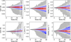 |
Fig. 16 As Fig. 15 but for two partially overlapping Gaussian components. |
| In the text | |
|
Fig. 17 MCMC error estimates for a two-component Gaussian fit. The synthetic spectrum consists of two Gaussian components and white noise with σT = 10% relative to the peak value in the spectrum. The corner plot shows the parameter correlations, where the colours of the 2D histogram correspond to the logarithm of probability (MCMC samples per pixel), as indicated by the colour bar on top. The red crosses correspond to the least-squares solution. The diagonal frames show the histograms for the individual parameters, and the dashed black and red lines correspond to the true values (before observational noise is added) and to the least squares fit, respectively. The frame on the right shows this particular fitted spectrum (black line) and the two components corresponding to the χ2 minimum. |
| In the text | |
|
Fig. 18 As Fig. 15 but for single-peaked synthetic C18O spectra selected from the MHD cloud model. The white lines show the average ±1-σ Monte Carlo error estimates. |
| In the text | |
|
Fig. 19 Example of hyperfine fits with degeneracy between the Tex and τ parameters. The upper frame shows χ2 values over a (Tex, τ) plane, with the χ2 minimum at the centre of the image (the white cross). The white and cyan contours correspond to a 1% and 40% increase over the minimum χ2. The bottom frame shows the spectrum (black line), the original model (spectrum without noise; red line), and the spectrum corresponding to the cyan cross in frame a (dashed cyan line). |
| In the text | |
|
Fig. 20 Comparison of parameter estimates from hyperfine fits with SPIF (red histograms; calculations in single precision) and with Scipy optimisation (blue histograms). The histograms are based on synthetic observations with a single velocity component and a relative noise that was varied between 1% and 20% of the peak value in the spectrum. The vertical dashed lines indicate the true values and the initial values used in the optimisation. The bottom frame shows the normalised χ2 values for each of the fitted spectra. |
| In the text | |
|
Fig. 21 Distribution of best-fit parameters and their error estimates in the case of synthetic N2H+ spectra from the cloud simulation. The sample consists of 100 spectra for each of the 322 noise levels. The black lines show the median parameter estimates, and the shaded red, blue, and grey areas correspond to the [20, 75], [10, 90], and [0.1, 99,9] percentiles of the parameter estimates, respectively. The median Monte Carlo error estimates are shown with solid white curves, and the 1-σ variation of the error estimates (between spectra at the same noise level) with cyan shaded regions. The error estimates are plotted symmetrically relative to the true parameter values. |
| In the text | |
|
Fig. 22 Comparison of parameter estimates from hyperfine fits with SPIF and with Scipy libraries. The figure is similar to Fig. 20 but for spectra with the higher total optical depth of τ = 10. |
| In the text | |
|
Fig. 23 Comparison of GaussPy (left frames) and SPIF (right frames) fits of the C180 spectra of the MHD model. The map resolution is R = 16 and the view direction x. The upper frames show the number of Gaussian components selected by the programs, with the fraction of spectra fitted with one to four components listed within the frames. The lower frames show the corresponding |
| In the text | |
|
Fig. 24 Sample C18O spectra from the MHD model, taken at equidistant positions over the area shown in Fig. 23. The black line shows the synthetic observations with noise equal to σ(T) = 0.05 K. The solid red and dashed blue curves correspond to the SPIF and GaussPy fits, respectively. The number of Gaussian components selected by the methods are indicated in the frames with numbers of the corresponding colour. |
| In the text | |
|
Fig. A.1 Statistics for synthetic C18O (upper row) and 13CO (bottom row) spectra. Histograms are plotted for the number of spectral peaks, the line width converted to standard deviation σ, the skewness, and the kurtosis. Each frame contains four histograms that correspond to R=1, 2, 8, and 32, in decreasing order of the histogram height. |
| In the text | |
|
Fig. C.1 Fit to spectra containing two Gaussian components and with noise varied from 1% to 30%. The upper frame shows the reduced χ2 values for GaussPy (blue line) and SPIF (red line) fits. The crosses indicate cases where programs have preferred the single-component fit. Some GaussPy fits have failed, and in those cases no χ2 value is plotted. In the case of GaussPy, we modelled the parameter using smoothing parameters α ~ δv for noise ≤ 16% and α ~ 40 × δv for noise > 16%. A fixed smoothing parameter for varying noise levels prevents GaussPy from isolating the multiple components. In the case of SPIF, both one-and two-component fits were performed and the model with the lower AIC values is included in the figure. The lower frame shows one example where GaussPy (blue line) has opted for a single-component fit, resulting in a noticeably higher χ1 value in frame a. |
| In the text | |
Current usage metrics show cumulative count of Article Views (full-text article views including HTML views, PDF and ePub downloads, according to the available data) and Abstracts Views on Vision4Press platform.
Data correspond to usage on the plateform after 2015. The current usage metrics is available 48-96 hours after online publication and is updated daily on week days.
Initial download of the metrics may take a while.