| Issue |
A&A
Volume 678, October 2023
|
|
|---|---|---|
| Article Number | A130 | |
| Number of page(s) | 27 | |
| Section | Interstellar and circumstellar matter | |
| DOI | https://doi.org/10.1051/0004-6361/202346102 | |
| Published online | 13 October 2023 | |
A global view on star formation: The GLOSTAR Galactic plane survey
VIII. Formaldehyde absorption in Cygnus X★
1
Max-Planck-Institut für Radioastronomie,
Auf dem Hügel 69,
53121
Bonn, Germany
e-mail: ygong@mpifr-bonn.mpg.de
2
Instituto Nacional de Astrofísica, Óptica y Electrónica,
Apartado Postal 51 y 216,
72000
Puebla, Mexico
3
Center for Astrophysics | Harvard & Smithsonian,
60 Garden St.,
Cambridge, MA
02138, USA
4
National Radio Astronomy Observatory,
1003 Lopezville RD,
Socorro, NM
87801, USA
5
Department of Astronomy, Faculty of Science, King Abdulaziz University,
PO Box 80203,
Jeddah
21589, Saudi Arabia
6
Xinjiang Astronomical Observatory, Chinese Academy of Sciences,
830011
Urumqi, PR China
7
Max Planck Institute for Astronomy,
Königstuhl 17,
69117
Heidelberg, Germany
8
IRAM,
300 rue de la piscine,
38406
Saint-Martin-d’Hères, France
9
Centre for Astrophysics and Planetary Science, University of Kent,
Canterbury
CT2 7NH, UK
10
National Astronomical Observatories, Chinese Academy of Sciences,
A20 Datun Road, Chaoyang District,
Beijing
100101, PR China
11
Key Laboratory of Radio Astronomy and Technology, Chinese Academy of Sciences,
A20 Datun Road, Chaoyang District,
Beijing
100101, PR China
12
Department of Earth and Space Science, Indian Institute for Space Science and Technology,
Trivandrum
695547, India
13
German Aerospace Center, Scientific Information,
51147
Cologne, Germany
14
National Radio Astronomy Observatory,
520 Edgemont Road,
Charlottesville, VA
22903, USA
15
Laboratoire d’astrophysique de Bordeaux, Univ. Bordeaux, CNRS, B18N,
allée Geoffroy Saint-Hilaire,
33615
Pessac, France
Received:
7
February
2023
Accepted:
31
July
2023
Context. Cygnus X is one of the closest and most active high-mass star-forming regions in our Galaxy, making it one of the best laboratories for studying massive star formation.
Aims. We aim to investigate the properties of molecular gas structures on different linear scales with the 4.8 GHz formaldehyde (H2CO) absorption line in Cygnus X.
Methods. As part of the GLOSTAR Galactic plane survey, we performed large-scale (7º×3º) simultaneous H2CO (11,0–11,1) spectral line and radio continuum imaging observations toward Cygnus X at λ ~6 cm with the Karl G. Jansky Very Large Array and the Effelsberg 100 m radio telescope. We used auxiliary HI, 13CO (1–0), dust continuum, and dust polarization data for our analysis.
Results. Our Effelsberg observations reveal widespread H2CO (11,0–11,1) absorption with a spatial extent of ≳50 pc in Cygnus X for the first time. On large scales of 4.4 pc, the relative orientation between the local velocity gradient and the magnetic field tends to be more parallel at H2 column densities of ≳1.8×1022 cm−2. On the smaller scale of 0.17 pc, our VLA+Effelsberg combined data reveal H2CO (11,0–11,1) absorption only towards three bright HII regions. Our observations demonstrate that H2CO (11,0–11,1) is optically thin in general. The kinematic analysis supports the assertion that molecular clouds generally exhibit supersonic motions on scales of 0.17−4.4 pc. We show a non-negligible contribution of the cosmic microwave background radiation to the extended absorption features in Cygnus X. Our observations suggest that H2CO (11,0–11,1) can trace molecular gas with H2 column densities of ≳5 × 1021 cm−2 (i.e., AV ≳ 5). The ortho-H2CO fractional abundance with respect to H2 has a mean value of 7.0 × 10⁻¹⁰. A comparison of the velocity dispersions on different linear scales suggests that the velocity dispersions of the dominant −3 km s−1 velocity component in the prominent DR21 region are nearly identical on scales of 0.17−4.4 pc, which deviates from the expected behavior of classic turbulence.
Key words: ISM: clouds / ISM: individual objects: Cygnus X / ISM: kinematics and dynamics / ISM: molecules / ISM: structure
The interactive 3D version of Fig. 7 is available at https://www.aanda.org
© The Authors 2023
 Open Access article, published by EDP Sciences, under the terms of the Creative Commons Attribution License (https://creativecommons.org/licenses/by/4.0), which permits unrestricted use, distribution, and reproduction in any medium, provided the original work is properly cited.
This article is published in open access under the Subscribe to Open model.
Open Access funding provided by Max Planck Society.
1 Introduction
Stars are the basic units of the Universe, but their formation is still one of the unsettled questions in modern astronomy. The Global View on Star Formation in the Milky Way (GLOSTAR1) survey is an unbiased survey of the interstellar medium (ISM) and star formation regions in the Milky Way using the wideband (4–8 GHz) C-band receivers of the Karl G. Jansky Very Large Array (VLA) and the Effelsberg 100 m telescope to simultaneously observe the radio continuum emission and selected spectral lines (Brunthaler et al. 2021). So far, the survey data have been used to characterize radio continuum sources (Medina et al. 2019; Nguyen et al. 2021; Dzib et al. 2023; Dokara et al. 2023), identify supernova remnants (Dokara et al. 2021, 2023), and search for methanol masers emitting in the 6.7 GHz transition, the strongest class II CH3OH maser line (Ortiz-León et al. 2021; Nguyen et al. 2022). This work is the first GLOSTAR study to investigate the ISM and star formation regions in the 4.8 GHz formaldehyde transition.
2 Formaldehyde as a tracer of molecular gas
Formaldehyde (H2CO) was the first polyatomic organic molecule to be discovered in the ISM (Snyder et al. 1969). Being a slightly asymmetric top molecule, its rotational energy levels are split into K doublets. This molecule has ortho- and para-symmetry species, depending on whether the spins of the hydrogen nuclei are parallel (ortho) or antiparallel (para). In molecular clouds, formaldehyde can be formed in the gas phase, but it is formed more efficiently on the surface of dust grains by successive hydrogenation of CO (Watanabe & Kouchi 2002), and is then released to the gas phase by thermal and nonthermal desorption.
The discovery of formaldehyde was made in the JKa,Kc = 11,0–11,1 doublet line of its ortho species near 4.8 GHz (6 cm) (Snyder et al. 1969). This line is generally observed in absorption against strong continuum background sources such as the Galactic center (Sgr A; Snyder et al. 1969), and even its hyper-fine structure (HFS) components have been detected in dark clouds (e.g., Heiles 1973). The ubiquity of absorption in this line is explained by the ease with which the lowest energy level of ortho-H2CO (JKa,Kc = 11,1) becomes overpopulated by collisional pumping, which results in a very low excitation temperature of <2.73 K for the lowest K-doublet transition of ortho-H2CO (11,0–11,1) (e.g., Evans et al. 1975). This overcooling results in absorption even against the cosmic microwave background (CMB).
The substantial electric dipole moment of H2CO of 2.33 D (Fabricant et al. 1977) makes its (sub)millimeter wavelength rotational transitions good probes of dense gas in star-forming regions. These properties have inspired several studies that used the rotational transitions of H2CO to probe the density and temperature of dense gas in the Milky Way and in external galaxies (e.g., Mangum & Wootten 1993; Ao et al. 2013; Ginsburg et al. 2015a; Tang et al. 2018a,b). On the other hand, H2CO has been observed in absorption against extragalactic continuum sources, indicating that H2CO can survive in diffuse and translucent molecular clouds (Nash 1990; Liszt & Lucas 1995; Menten & Reid 1996; Snow & McCall 2006; Liszt et al. 2006). This ease with which the ortho-H2CO (11,0–11,1) transition is excited in diffuse and translucent clouds suggests that it traces the largest extent of molecular gas when compared with other H2CO transitions. These facts pose the question to which extent this H2CO transition can trace the general distribution of molecular gas. In order to address this question, large-scale mapping observations of H2CO are required, but such observations are still scarce. Large-scale mapping studies of H2CO (11,0–11,1) absorption have been performed toward the central molecular zone (Zylka et al. 1992), W51 (Ginsburg et al. 2015a), and the Aquila molecular cloud (Komesh et al. 2019), revealing a widespread distribution of H2CO in these regions. However, these observations mainly focused on high H2 column density (i.e., high-extinction) molecular gas, and the maps cover less than 5 square degrees in total.
Because the (11,0–11,1) and (21,1–21,2) pair of H2CO lines have been proven to be a good densitometer (e.g., Henkel et al. 1980; Mangum & Wootten 1993; Mangum et al. 2008), large-scale H2CO (11,0–11,1) mapping observations are able to pinpoint regions with appreciable absorption, which can facilitate follow-up H2CO (21,1–21,2) imaging for density determinations of molecular clouds on large scales. For instance, this method has been applied to the W51 cloud (e.g., Ginsburg et al. 2015a).
Based on the large coverage of the GLOSTAR observations, our survey can potentially reveal the distribution of H2CO (11,0–11,1) absorption on a Galactic scale for the first time (Brunthaler et al. 2021). In this work, we present the first results based on GLOSTAR measurements of H2CO in Cygnus X.
3 Cygnus X as an excellent astrophysical laboratory
Cygnus X, named by Piddington & Minnett (1952), is one of the closest and most active high-mass star-forming regions in the Milky Way (e.g., Reipurth & Schneider 2008; Kryukova et al. 2014). This region exhibits very extended bright Galactic radio continuum emission that arises from discrete HII regions, supernova remnants (SNRs), and diffuse thermal emission (Wendker 1984; Wendker et al. 1991; Xu et al. 2013a; Emig et al. 2022). Cygnus X contains several OB associations that harbor a large number of massive stars (Knödlseder 2000; Wright et al. 2015; Berlanas et al. 2018). Observations have also shown that a large X-ray bubble and very high energy γ-rays were found to surround one of the most prominent of these stars, Cyg OB2 (e.g., Cash et al. 1980; Abeysekara et al. 2021; Cao et al. 2021b). By the irradiation from the Cyg OB2 association, pillars and globules are formed in ambient molecular clouds with an orientation toward the center of the Cyg OB2 association (Schneider et al. 2016, 2021), demonstrating the role of the feedback of OB stars in shaping molecular clouds.
The distance of Cygnus-X has been a subject of considerable debate. Because molecular cloud complexes in Cygnus X seem to be associated with each other due to the coherence in line-of-sight velocities (Schneider et al. 2006), a fixed distance of about 1.4–1.7 kpc is commonly assumed for all molecular clouds in this region by many previous studies. While this is consistent with the results of accurate trigonometric parallaxes of maser sources located in various parts of Cygnus X and massive stars in the Cygnus OB2 association (Rygl et al. 2012; Xu et al. 2013b; Dzib et al. 2013), later studies also found sources at farther distances of 3.3–3.6 kpc (Rygl et al. 2012; Xu et al. 2013b) and even ≳9 kpc (indicated by the radial velocity of < −60 km s−1; Lockman 1989; Ortiz-León et al. 2021; Li et al. 2021a). However, studies using the Gaia parallax measurements and their line-of-sight extinctions suggest that the bulk of molecular gas should be located at 1.3–1.5 kpc in Cygnus X (Zucker et al. 2020; Chen et al. 2020; Dharmawardena et al. 2022). For simplicity, we adopt a distance of 1.4 kpc in this work, and the values of physical parameters obtained from previous studies are scaled to this distance for comparison.
Cygnus X harbors one of the most massive molecular cloud complexes (~2–3 × 10⁶ M⊙) identified in the Milky Way (Schneider et al. 2006). Previous CO and dust continuum observations show a highly structured distribution of molecular clouds (e.g., Schneider et al. 2006; Hennemann et al. 2012; Cao et al. 2019) and filamentary structures in Cygnus X. The filaments, especially toward the prominent compact HII region DR21 and its environment, are found to show velocity gradients (Schneider et al. 2010; Hu et al. 2021; Cao et al. 2022; Li et al. 2023; Bonne et al. 2023), indicating ongoing accretion flows on subparsec scales. A large number of dense cores and massive protostars are found in these filaments (including DR21; Motte et al. 2007; Schneider et al. 2011; Bontemps et al. 2010; Roy et al. 2011; Hennemann et al. 2012; Cao et al. 2019; Cheng et al. 2022; Ching et al. 2022). In one of these studies, Cao et al. (2019) built a large sample of 151 massive dense cores that have masses of >35 M⊙ with a typical size of ~0.1 pc. Their further efforts led to the identification of a sample of 8,431 dust cores (Cao et al. 2021a). Based on these results, the large-scale density structure is studied with a triangulation-based method (Li et al. 2021b), implying that dense cores form through fragmentation controlled by scale-dependent turbulent pressure support.
As part of the GLOSTAR survey, Ortiz-León et al. (2021) detected thirteen 6.7 GHz methanol masers in Cygnus X that are exclusively associated with high-mass young stellar objects. Further evidence of widespread star formation activity in these sources is provided by the discovery of about 60 molecular outflows in Cygnus X in large-scale CO surveys (Gottschalk et al. 2012; Duarte-Cabral et al. 2013; Deb et al. 2021; Skretas & Kristensen 2022). These properties make Cygnus X one of the best laboratories for studying massive star formation. The Cygnus X region is therefore targeted by many ongoing large-scale projects, including GLOSTAR (Brunthaler et al. 2021), the K-band focal plane array Examinations of Young STellar Object Natal Environments (KEYSTONE; Keown et al. 2019), the Surveys of Clumps, CorEs, and CoNdenSations in CygnUS-X (CENSEUS; Cao et al. 2019), and the Cygnus Allscale Survey of Chemistry and Dynamical Environments (CASCADE; Beuther et al. 2022). Therefore, the study of H2CO absorption in Cygnus X will pave the way toward understanding gas distribution, kinematics, chemistry, and evolutionary processes associated with high-mass star formation.
4 Observations and data reduction
4.1 Effelsberg 100 m observations
As part of the GLOSTAR survey (Brunthaler et al. 2021), we performed C-band observations with the dual-polarization S45mm receiver of the 100 m telescope near Effelsberg in Germany2 between 2019 January 11 and 2020 December 23 (project codes: 22-15 and 102-20). The observations and data reduction were described in Brunthaler et al. (2021), and the calibration quality of the Effelsberg spectral line observations will be discussed in Rugel et al. (in prep.). In the following, we summarize the observations and data products relevant to this publication. Two different kinds of backends, the SPEctro-POLarimeter (SPECPOL) and fast Fourier transform spectrometers (FFTSs; Klein et al. 2012), were used to record full Stokes continuum emission and spectral line signals, respectively. The on-the-fly (OTF) mode was used to map Cygnus X with a scanning speed of 90″ per second. Like all of the area covered by GLOSTAR, the region has been mapped in both Galactic longitude and latitude in order to reduce striping artifacts in the image restoration. Our observations cover an area of 7° × 3° in size (i.e., 76° ≤ l ≤ 83°, −1°≤ b ≤2°). The flux calibrators 3C 286 and NGC 7027 were used to establish the flux density scale of both our radio continuum and spectral line data. The system temperatures typically range from 28 to 42 K. Nearby pointing observations were carried out every 2 to 3 h. The rms pointing uncertainty was found to be within 10″, which is less than one-tenth of the half power beam width (HPBW) of 145″ at 4.83 GHz.
We have used the Effelsberg data to study the large-scale ISM structure of Cygnus X in the 4.8 GHz formaldehyde transition, while the associated 4.89 GHz continuum data were used to derive the optical depth of the H2CO line emission. In our setup, we simultaneously covered H2CO (11,0–11,1) at 4.8296600 GHz and its isotopolog  CO (11,0–11,1) at 4.5930885 GHz (Müller et al. 2005; Endres et al. 2016). The channel spacings for H2CO (11,0–11,1) and
  CO (11,0–11,1) were 0.19 km s−1 and 2.49 km s−1 (see Table 2 in Brunthaler et al. 2021), respectively. All the velocities are given with respect to the local standard of rest (LSR). Spectral data were preprocessed and calibrated with the standard Effelsberg pipeline, which includes bandpass and absolute intensity calibration (Winkel et al. 2012), as well as a correction for atmospheric attenuation based on a water-vapor radiometer operating between 18 and 26 GHz. Because the spectra were regridded using Gaussian convolution in the pipeline, the actual spectral resolution corresponds to two channel widths (e.g., 0.38 km s−1 for the 4.8 GHz H2CO line). Further data reduction and mapping of the data was performed with the GILDAS3 software (Pety 2005). Six out of 1946700 H2CO spectra were affected by radio frequency interference (RFI) and were thus discarded in the data reduction. The spectral baseline subtraction was carried out using a first-order polynomial.
Our spectral map was first convolved to an effective HPBW of 3′ with a single pixel size of 30″× 30″. However, at this spatial resolution, the signal-to-noise ratio of the H2CO image was not sufficient to detect the extended absorption. To improve the fidelity of the extended absorption, the data were further convolved to an effective angular resolution of 10′.8.
The spatial distribution of the rms noise values is shown in the top panel of Fig. 1. The rms noise can vary by a factor of 2 because of different effective integration times. We also illustrate the 2D power spectra in the lower left panel of Fig. 1. The power spectrum shows that there is no clear correlation at any specific spatial scale. The lower right panel of Fig. 1 presents the histogram of the rms noise values, which range from 0.07 to 0.24 K with a median value of 0.10 K at a channel width of 0.5 km s−1.
The simultaneously observed 4.89 GHz radio continuum data were reduced with the NOD3 software package (Müller et al. 2017). The typical rms noise levels are 5 mK at a narrow bandwidth of 120 MHz. As described in Brunthaler et al. (2021), the zero-level intensities of our Effelsberg data needed to be restored using the Urumqi 4.8 GHz continuum data (Sun et al. 2007, 2011). However, the zero-level intensities of the Urumqi 4.8 GHz continuum data of Cygnus X need to be restored as well because the radio continuum emission of Cygnus X is very extended, reaching |b| > 5°. For this reason, we made use of model c from the WMAP foreground maps4 (Bennett et al. 2013). We derived the WMAP-based 4.8 GHz continuum emission by interpolating the free-free, synchrotron, and dust emission. Smoothing the WMAP-based and Urumqi 4.8 GHz continuum images to a common angular resolution of 1.°5, we derived the zero-level shift of the Urumqi 4.8 GHz data from the difference between the derived WMAP-based and Urumqi 4.8 GHz continuum images. The difference ranges from −0.065 K to 0.269 K, which is a small correction. These differences were then added back to the original Urumqi 4.8 GHz continuum image. Our Effelsberg 4.89 GHz data cover only −1º< b < 2°, and thus have a zero-level shift due to the continuum baseline correction only covering the limited range of Galactic latitude. Following the same method introduced in Brunthaler et al. (2021), we used the restored Urumqi 4.8 GHz data to recover the zero4evel shift of our Effelsberg 4.89 GHz data. Consequently, the restored Effelsberg 4.89 GHz continuum map was used in this study.
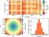 |
Fig. 1 Noise distribution and statistical results. Top: Spatial distribution of the rms noise of the Effelsberg H2CO (11,0–11,1) observations at a channel width of 0.5 km s−1 and an HPBW of 3′. Lower left: Power spectrum of the noise image. The very high power pixels in the cross are artifacts that are caused by the Fourier transform of the sharp image (also known as the Gibbs phenomenon). Lower right: Histogram of the rms noise values. The mean and standard deviation values are 0.10 K and 0.01 K, respectively. |
4.2 VLA observations
As part of the GLOSTAR survey (Medina et al. 2019; Brunthaler et al. 2021), the Cygnus-X region was observed using the D configuration of the Karl G. Jansky Very Large Array (VLA) of the National Radio Astronomy Observatory5 with the correlator configuration including the H2CO line. Details of the observations have been presented in Ortiz-León et al. (2021); here we give a brief summary. We observed 14 strips of 1 º × 1.5 º in size that cover the same area as the Effelsberg observations. The observations registered sixteen 128 MHz wide spectral windows for the continuum. The H2CO (11,0–11,1) line was observed simultaneously with a bandwidth of 4 MHz and 1024 channels, resulting in a channel spacing of 0.25 km s−1 and in a total velocity coverage of 260 km s−1. The spectral line data were calibrated using the Common Astronomy Software Applications (CASA) package (McMullin et al. 2007) using a customized version of the VLA pipeline6. The line imaging was performed for each strip using the mosaic mode in CASA and a pixel size of 2″.5×2″.5. The synthesized beam is about 19″×15″ with a position angle of −34° for H2CO (11,0–11,1). The largest angular scale structure that our VLA D array observations is sensitive to is about 4′.
The radio continuum emission was calibrated and imaged using the Obit package (Cotton 2008); see Brunthaler et al. (2021) for more details. For the analysis presented here, we only used a ~200 MHz wide frequency sub-band centered at 4.9 GHz out of the 16 spectral windows. The continuum image has a circular beam of 19″and a pixel size of 2″.5×2″.5. In order to match the angular resolution of the continuum and line emission, we smoothed the two VLA data sets to a circular beam of 25″ for our analysis.
4.3 Combination of VLA and Effelsberg data
Because the VLA D configuration data lack short-spacing information, we combined the VLA and Effelsberg data in order to recover the extended emission and absorption. As illustrated in Brunthaler et al. (2021), there is no clear systematic offset between the VLA and Effelsberg flux calibration. Hence, no flux scaling was needed. Before the combination, we regridded the VLA and Effelsberg H2CO data sets to the same channel width of 0.5 km s−1. The combination was performed with the feather task in CASA. The combined data have a circular beam of 25″ for both the continuum and the H2CO (11,0–11,1) spectral line images, which corresponds to a linear scale of ~0.17 pc in Cygnus X. The typical 1σ noise level is about 20 mJy beam−1 (or 1.7 K in units of brightness temperatures) at a channel width of 0.5 km s−1.
We compare the VLA-only and VLA+Effelsberg combined data toward DR22 in Fig. 2. While the distributions are similar in both data sets, it is evident that the VLA+Effelsberg combined data show more extended emission and higher flux densities, which confirms that the combined data recover the missing flux in the VLA D-configuration data. Therefore, we adopted the VLA+Effelsberg combined data for the following analysis on small scales.
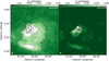 |
Fig. 2 Comparison of the 4.9 GHz radio continuum maps of DR22 from the VLA+Effelsberg combined and VLA-only data sets. In both panels, the contours start from 0.02 Jy beam−1 and increase by 0.02 Jy beam−1. The beam size is shown in the lower left corner of each panel. |
4.4 Archival data
In order to determine the H2 column density in Cygnus X, we used the Planck 353 GHz map of the dust optical depth, which was derived by fitting the spectral energy distribution (SED) of dust emission inferred from continuum maps ranging from 353 to 3000 GHz (Planck Collaboration XI 2014). The conversion factor from the 353 GHz dust optical depth into the H2 column density is discussed in Sect. 6.2. The HPBW was 4′.9. The Planck thermal dust polarization data at 353 GHz were used to study the polarization properties of molecular clouds in Cygnus X (Planck Collaboration Int. XX 2015; Planck Collaboration Int. XIX 2015). The data were smoothed to 10′ to achieve a signal-to-noise ratio greater than 3 in the amplitude of linear polarization. These maps were obtained from the public Planck Legacy Archive7.
We also used 13CO (1–0) data obtained from the Five College Radio Astronomical Observatory (FCRAO), the details of which were described in Schneider et al. (2011). The HPBW was 46″, and the channel spacing was 0.066 km s−1. The typical 1σ rms noise level was 0.2 K per channel on an antenna temperature scale. A main beam efficiency of 0.48 was adopted in this study.
A HI column density map was obtained from the Effelsberg-Bonn HI Survey (EBHIS; Kerp et al. 2011; Winkel et al. 2016). The HPBW was 10′.8 at 1.420 GHz. The rms noise level was 90 mK at a channel spacing of 1.29 km s−1.
5 Results
5.1 Widespread formaldehyde absorption
5.1.1 Overall distribution
The 4.8 GHz formaldehyde transition is typically observed in absorption. A sample spectrum is shown in Fig. 3, where the two velocity components at −3 km s−1 and 8 km s−1 arise from the DR2l cloud and its foreground cloud associated with W75N (e.g., Cyganowski et al. 2003; Schneider et al. 2010; Dobashi et al. 2019), respectively. Figure 4 shows the distribution of the H2CO intensity integrated over the velocity range between −10 km s−1 and 20 km s−1 at an angular resolution of 10′.8. Although H2CO (11,0–11,1) has been investigated toward several positions in Cygnus X (e.g., Bieging et al. 1982; Henkel et al. 1983; Piepenbrink & Wendker 1988; Yan et al. 2019), our Effelsberg 100 m observations reveal the widespread nature of H2CO absorption in Cygnus X for the first time. With an area coverage of 21 square degrees, this is the largest H2CO (11,0–11,1) map of the region to date.
Figure 5 shows the Effelsberg 4.89 GHz radio continuum image overlaid with the peak H2CO absorption contours at two different angular resolutions (i.e., 3′ and 10′.8). The widespread absorption is mainly attributed to two main structures known as CygX-North and CygX-South (labeled in the top panel of Fig. 4) following the nomenclature by Schneider et al. (2006, 2011).
Figure 5 shows that the absorption toward CygX-North covers an area ~2º × 2º, in which several discrete absorption peaks are superimposed on more diffuse absorption. In CygX-South, the absorption covers a larger area with a similar diffuse morphology, onto which more compact peaks are superimposed. The extended absorption is more evident in Fig. 5b than in Fig. 5a because the larger beam size of the former makes it much more sensitive to extended absorption. The lowest contour in Fig. 5b suggests a total area of approximately 4700 pc2 for the detectable H2CO (11,0–11,1) absorption.
In Fig. 5, strong H2CO absorption features coincide with the bright radio continuum emission from (most prominently) DR21, DR17, DR22, DR6, W69, and G078.177-00.363. This is due to enhancements of the amplitude of absorption (in units of main beam temperature) against the bright continuum emission. The strongest H2CO absorption arises from the line of sight toward DR21, which is largely due to the fact that DR21 is the brightest radio continuum source in this field (see Fig. 3). This is consistent with previous pointed observations (Piepenbrink & Wendker 1988). However, many of the extended H2CO absorption features are not associated with bright compact radio continuum sources in Fig. 5b.
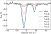 |
Fig. 3 Observed H2CO (11,0–11,1) spectrum at an HPBW of 10′.8 toward DR21 (solid black line) overlaid with the fitted model (solid blue line). The two velocity components at −3 km s−1 and 8 km s−1 correspond to two physically distinct velocity components that arise from the DR21 cloud and its foreground cloud associated with W75N. The fitted HFS components are indicated by the colored dashed lines in the legend. |
5.1.2 Optical depth
Based on the radiative transfer equation in the Rayleigh-Jeans regime, the main beam temperature, Tmb, can be expressed as
 (1)
(1)
where Tex is the excitation temperature, Tbg is the temperature of the CMB radiation that is taken to be 2.73 K (e.g., Fixsen 2009), and Tc is the brightness temperature of the continuum emission behind the H2CO gas, fb is the beam dilution factor, and τ is the optical depth.
Measurements of the HFS components of H2CO (11,0–11,1) give an excitation temperature of ~1.6 K in dark clouds (e.g., Heiles 1973). However, this method can only be applied to cases where the line widths are narrow enough. Our spectra are too broad to resolve the HFS components, so we have to assume excitation temperatures for our study. In addition to the HFS measurements (e.g., Heiles 1973), statistical equilibrium calculations suggest that the excitation temperatures are typically 1.2–1.8 K in massive star-forming regions (Henkel et al. 1980; Yan et al. 2019). This suggests that the excitation temperature does not change significantly in different regions, and consequently, we assumed a constant Tex of 1.6 K for our analysis (see also Sect. 6.2). If the excitation temperature varies in the range of 1.2–2.0 K, this assumption results in uncertainties of 25% in the derived optical depth at most.
In order to estimate the H2CO optical depth, we assumed that all the observed radio continuum emission lies behind the molecular gas. Hence, the observed radio continuum emission in Fig. 5 contributes to Tc in Eq. (1). Because of the widespread H2CO distribution (see Sect. 5.1.1), fb is simply assumed to be unity to estimate τ. Figure 6 shows the derived peak optical depth distribution at angular resolutions of 3′ and 10′.8. The peak optical depth values are found to be lower than unity at all locations. The optical depths at an angular resolution of 3′ are generally higher than those at 10′.8 resolution. For the angular resolution of 10′.8, all the peak optical depth values are lower than 0.4. The maximum τ of ~0.34 is located in the region centered at l = 77.877º, b = 0.865º. This suggests that H2CO (11,0–11,1) is optically thin at almost all locations. We also note that the optical depth would be underestimated if only a small fraction of the radio continuum emission were to contribute to the background emission in Eq. (1). However, optical observations have shown that Cygnus X is seen as a dark patch in the sky (see, e.g., Fig. 1 in Schneider et al. 2006), which suggests that most radio continuum emission from the HII regions should lie behind the molecular clouds. Toward the same line of sight, the H2CO gas behind the radio continuum emission is likely weaker than the H2CO gas in the front because the absorption can be enhanced against radio continuum emission. Therefore, the derived optical depths are likely reliable.
The column density of H2CO in the upper energy level,  , can be estimated from the optical depth using the following formula (Eq. (30) in Mangum & Shirley 2015):
![${N_{{1_{1,0}}}} = {{3h} \over {8{h^3}\mu _{{\rm{lu}}}^2}}\,{\left[ {{\rm{exp}}\,\left( {{{hv} \over {k{T_{{\rm{ex}}}}}}} \right) - 1} \right]^{ - 1}}\,\,\int {\tau \,{\rm{d}}\upsilon } ,$](/articles/aa/full_html/2023/10/aa46102-23/aa46102-23-eq5.png) (2)
(2)
where h is the Planck constant, µlu is the dipole moment of 2.33 D (Fabricant et al. 1977), and k is the Boltzmann constant. Assuming a constant Tex of 1.6 K, Eq. (2) becomes
 (3)
(3)
Integrating the optical depth over the velocity range from −10 km s−1 to 20 km s−1, we derived the H2CO column density at the 11,0 level with Eq. (3), and the results are presented in Fig. 6c. The H2CO column densities range from 3 × 10¹¹ to 9.0 × 1012 cm−2 with a median value of 2.9 × 1012 cm−2 at the 11,0 level. We note that variations in the excitation temperatures can affect the accuracy of the column density determination. If the expected excitation temperatures vary from 1.2 to 2 K, the assumption of constant excitation temperature lead to an uncertainty of a factor of ~2 in the derived  . Based on the method introduced in Appendix A, we derived that the total ortho-H2CO column density ranges from 8 × 10¹¹ to 2.3 × 1013 cm−2 with a median value of 7.4 × 1012 cm−2.
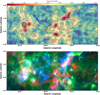 |
Fig. 4 Distribution of molecular and ionized gas in Cygnus X. Top: integrated-intensity map of the Effelsberg H2CO (11,0–11,1) absorption at an HPBW of 10′.8. The integrated velocity range extends from −10 to 20 km s−1. The contours start at −0.4 K km s−1 (5σ), with each subsequent contour being twice the previous one. The overlaid pattern indicates the magnetic field direction based on the polarization measurements by the Planck satellite (Planck Collaboration XI 2014) created by the line integral convolution (LIC) method (Cabral & Leedom 1993). Bottom: overview of the Cygnus X region in a three-color composite image with the Effelsberg H2CO (11,0–11,1) absorption at an HPBW of 10′.8 shown in red, MSX 8 µm image in green, and the Effelsberg 4.89 GHz continuum emission plotted in blue. |
5.1.3 Decomposition
The H2CO (11,0–11,1) transition is comprised of six HFS lines (e.g., Tucker et al. 1971). The overlapping HFS lines might introduce uncertainties in the fitted velocities and line widths. We therefore performed a simulation to study the impact of the HFS lines to test the effects. The results, which are presented in Appendix B, demonstrate that the velocity centroid derived by Gaussian fitting can have an intrinsic velocity shift of −0.12 km s−1 to 0.03 km s−1 and the line widths can be overestimated by approximately a factor of 1.5–2.5. In order to properly decompose the H2CO spectra, we simultaneously fit six Gaussian components to the observed spectra on the basis of the rest frequencies and relative line strengths of the six HFS lines (Müller et al. 2005) using the LMFIT8 python package (Newville et al. 2014). Because most of the H2CO (11,0–11,1) absorption is expected to be optically thin (see the discussion in Sect. 5.1.2), the method should be valid across the whole region.
In regions with multiple velocity components, first, the brightest H2CO absorption component along the line of sight was fit, which was followed by fitting an additional component to the residual if significant. We repeated this process until the peak residual absorption was no brighter than 5σ. The chosen threshold allowed us to avoid fit results with low confidence levels. As an example, Fig. 3 presents the two-component fitting to the spectrum along the line of sight toward DR21. Figure 7 shows the fitted results for the complete H2CO distribution in Cygnus X covered by us. From its upper panel, it is evident that the fitted velocities are between −7 km s−1 and 15 km s−1. The lower panel of Fig. 7 suggests that the velocity dispersions are within the range of 0.16−4.04 km s−1 with a median value of 1.07 km s−1. These are consistent with early statistical results of 34 positions in Cygnus X (Piepenbrink & Wendker 1988).
Before investigating the velocity information, we first applied the clustering algorithm, density-based spatial clustering of applications with noise (DBSCAN9, e.g., Ester et al. 1996; Schubert et al. 2017; Yan et al. 2020), to the fitted results (coordinates, LSR velocities, and velocity dispersions) in order to assign the observed absorption to different coherent cloud structures. The algorithm requires two parameters, ϵ and pmin. ϵ corresponds to the maximum distance between two samples for one to be considered as being in the neighborhood of the other, while pmin represents the minimum number of points required to form a coherent region. We used twice the number of dimensions (i.e., four, considering that the four dimensions correspond to Galactic longitude, Galactic latitude, LSR velocity, and velocity dispersion) of our data as pmin. The results of the clustering algorithm depend sensitively on ϵ, with higher values of ϵ leading to more extended cloud structures (see the discussions in Appendix C). Because we only intend to study extended cloud structures that are well resolved at an angular resolution of 10′.8, we manually increased ϵ to 0.25 (see the discussions in Appendix C). Consequently, we detected eight coherent and extended cloud structures that are well resolved at the angular resolution of 10′.8. The results are shown in Fig. 8. The cloud structures, labeled A to H, cover areas of 51–1055 pc2. Cloud E in CygX-South is the most extended and coherent cloud structure.
In Fig. 8, three cloud structures (i.e., A, F, and H) overlap along the line of sight in CygX-North, while two cloud structures (i.e., E and G) overlap along the line of sight toward CygX-South. In CygX-North, the three cloud structures are characterized by LSR velocities of −3 km s−1, 5 km s−1, and 8 km s−1. Based on previous studies (e.g., Cyganowski et al. 2003; Schneider et al. 2010; Dobashi et al. 2019), the −3 km s−1 component (i.e., H) mainly stems from the molecular gas associated with DR21, while the 8 km s−1 component (i.e., F) arises from the W75N component in front of molecular clouds associated with DR21. Previous studies suggested that the interaction between the two components may trigger massive star formation in this region (e.g., Dickel et al. 1978; Dobashi et al. 2019). The 5 km s−1 cloud (i.e., A) is connected to clouds F and H in both spatial and velocity spaces, which implies that cloud F is also interacting with the other two clouds. Toward CygX-South, clouds E and G also overlap along the line of sight, although we do not see signatures of massive star formation at the intersection.
The fitted LSR velocity centroids appear to show ordered velocity gradients, and these gradients are further discussed in Sect. 6.4. Figure 9 presents the statistics of the velocity dispersions for the eight cloud structures, which have a median value of 1.04 km s−1. The observed velocity dispersions, σv, consist of contributions from thermal and nonthermal motions, σt and σnt,
 (4)
(4)
The thermal velocity dispersion can be estimated from the following relation:
 (5)
(5)
where k is the Boltzmann constant, Tk is the kinetic temperature, and mi is the mass of the molecule (e.g., mi = 30 for H2CO). Because molecular clouds have typical kinetic temperatures of 10 K, the characteristic thermal velocity dispersion is 0.05 km s−1. As is evident from Fig. 9, the observed velocity dispersions are much higher than 0.05 km s−1, suggesting that the molecular gas in Cygnus X is dominated by nonthermal motions on a 4.4 pc (i.e., 10.′ 8) scale. The Mach number is defined as
 (6)
(6)
where cs is the sound speed of molecular gas. cs is 0.19 km s−1 at Tk = 10 K, where the mean molecular weight is taken to be 2.37 (Kauffmann et al. 2008). Figure 9 suggests that most of the molecular gas traced by H2CO absorption has ℳ > 2, which is indicative of nearly ubiquitous supersonic motions in Cygnus X.
The minimum Mach number could be slightly overestimated because of the spectral dilution. Our minimum velocity dispersion is about 0.5 km s−1, which corresponds to a Gaussian line width of ~1.2 km s−1. Taking the spectral dilution caused by the 0.5 km s−1 channel into account, the broadening line width becomes 1.3 km s−1, which is about 8% broader than the intrinsic value. Therefore, the spectral dilution does not play a crucial role.
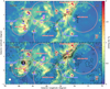 |
Fig. 5 Radio continuum emission and H2CO absorption seen by the Effelsberg 100 m telescope. (a) Effelsberg 4.89 GHz radio continuum emission overlaid with the peak absorption contours of H2CO (11,0–11,1). The corresponding HPBW of H2CO (11,0–11,1) is 3′. The color bar represents the flux densities of the radio continuum emission. The H2CO absorption contours start from −0.5 K (5σ) and decrease by 0.5 K. The developed HII regions from Anderson et al. (2014) are marked with solid red circles, and SNR G78.2+2.1 is indicated by the dashed orange circle. Blue crosses represent the radio continuum sources and active star-forming objects, and the purple star represents the massive star cluster, Cygnus OB2. (b) Similar to Fig. 5a, but the corresponding HPBW of H2CO (11,0–11,1) is 10′.8. The H2CO absorption contours start from −0.08 K (4σ) and decrease by 0.06 K. In both panels, the beam size is shown in the lower left corner. |
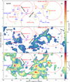 |
Fig. 6 Distribution of the physical properties derived from H2CO (11,0–11,1). (a) Distribution of the peak optical depth of the H2CO (11,0–11,1) line. The HPBW of the H2CO image is 3′. The color bar represents the peak optical depth. The HII regions from Anderson et al. (2014) are marked with solid red circles, and SNR G78.2+2.1 is indicated by the dashed orange circle. The blue crosses represent the radio continuum sources and active star-forming objects, and the purple star represents the massive star cluster, Cygnus OB2. (b) Similar to Fig. 6a, but the HPBW of the H2CO (11,0–11,1) image is 10′.8. (c) Similar to Fig. 6b, but for the H2CO column density at the 11,0 level. In all panels, the beam size is shown in the lower left corner. |
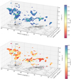 |
Fig. 7 3D view of the decomposition of the observed H2CO (11,0–11,1) spectra in Cygnus X. The line of sight toward DR21 is indicated by the dashed black line. The upper panel shows the distribution of the fitted intensity. The H2CO (11,0–11,1) peak absorption contours are shown at the base of the plot, and the contours are the same as shown in Fig. 5. The lower panel shows the velocity dispersion distribution. The interactive version of this 3D view is available online and via the links (top: high sampling: https://gongyan2444.github.io/3D/cyg-h2co-amp.html, low sampling: https://gongyan2444.github.io/3D/cyg-h2co-amp-low.html; bottom: high sampling: https://gongyan2444.github.io/3D/cyg-h2co-dis.html, low sampling: https://gongyan2444.github.io/3D/cyg-h2co-dis-low.html). |
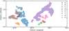 |
Fig. 8 Eight coherent cloud structures derived from the DBSCAN algorithm. The different structures are labeled with different colors. The cross marks the position of DR21. |
5.2 Formaldehyde absorption on small scales
Our GLOSTAR VLA D array observations provide the first unbiased H2CO (11,0−11,1) absorption survey toward Cygnus X on a scale of ~0.17 pc. This has led to the robust detection (≥5σ) of H2CO (11,0−11,1) absorption toward three compact radio continuum sources, DR21, DR22, and G76.1883+0.0973 (also known as IRAS 20220+3728), which are known to be Hii regions (e.g., Gregory & Condon 1991; Kurtz et al. 1994; Motte et al. 2007). The sparse number of absorption detections toward compact sources is mainly attributed to our sensitivity: Based on our 1σ sensitivity of about 0.02 Jy beam−1 (or 1.7 K) at a channel width of 0.5 km s−1, only strong absorption features can be detected by our observations.
As shown in Fig. 10, these bright H2CO (11,0−11,1) absorption distributions match the distributions of the 4.9 GHz radio continuum emission, which strongly supports the hypothesis that these features are due to absorption of continuum emission (as opposed to the CMB). DR21, DR22, and G76.1883+0.0973 are well-known massive star formation regions (e.g., Motte et al. 2007; Ortiz-León et al. 2021). Therefore, all the absorption features detected by the high angular resolution data are in the direction of massive star-forming regions.
As is evident in Fig. 10a, the spectrum toward DR21 exhibits two velocity components at −3 km s−1 and 8 km s−1. Their distributions show that both components are against the radio continuum emission of DR21 (see Fig. 10b). The −3 km s−1 component has a higher optical depth than the 8 km s−1 component, which can explain the fact that the 8 km s−1 component was not detected by previous NH3 (1,1) and 6.7 GHz methanol line observations (Cyganowski et al. 2003; Ortiz-León et al. 2021). The −3 km s−1 component was also detected in absorption in the 1667 MHz OH and 6.7 GHz CH3OH lines (see Fig. 8 in Ortiz-León et al. 2021), but the blueshifted wing-like features detected in the 1667 MHz OH and 6.7 GHz CH3OH lines are absent in H2CO (11,0−11,1).
In Fig. 10, we also compare the H2CO (11,0−11,1) LSR velocities with the LSR velocities of the three HII regions derived from radio recombination line (RRL) observations at a similar angular resolution (Khan et al., in prep.). The velocity differences are 0.5 ± 0.3 km s−1, 15.5 ± 0.2 km s−1, and 5.2 ± 0.8 km s−1 for DR21, DR22, and G76.1883+0.0973, respectively. We find that the molecular gas is redshifted with respect to the RRL velocities at least toward DR22 and G76.1883+0.0973. The presence of H2CO (11,0−11,1) absorption suggests that the molecular gas lies in front of the HII regions. The large velocity differences indicate that the molecular gas is likely not associated with the ionized gas for the two HII regions.
Following the same method as we used in Sect. 5.1.2, we also derived the H2CO optical depths in the VLA data (see Fig. 10). All the derived optical depth values are lower than 0.8. The line of sight toward G76.1883+0.0973 has the highest optical depth of all detections, ~0.7. It is worth noting that G76.1883+0.0973 does not reside in the bright cloud structures of CygX-North and CygX-South (see Fig. 5). We also derived the H2CO column densities at the 11,0 level, which range from 4.2 × 10¹² to 7.3 × 1013 cm−2 with a median value of 6.8 × 1012 cm−2.
In order to study the kinematics, we also decomposed the VLA+Effelsberg data as in Sect. 5.1.3. Because two velocity components at −3 km s−1 and 8 km s−1 are evident toward DR21 in Fig. 10, we investigated them separately. Figure 11 shows a histogram of the velocity dispersions for the four components in the three regions. The distributions have mean values of 1.61 km s−1, 0.91 km s−1, 0.68 km s−1, and 0.60 km s−1 for the −3 km s−1 component of DR21, the 8 km s−1 component of DR21, DR22, and G76.1883+0.0973, respectively. Based on previous ammonia observations, kinetic temperatures range from 17 to 28 K around DR21 and DR22 (Keown et al. 2019), which corresponds to thermal H2CO velocity dispersions of 0.07–0.09 km s−1. It is evident that the observed velocity dispersions are much higher than what is expected from thermal motion. Hence, they are dominated by nonthermal motion (i.e., turbulence). Furthermore, the −3 km s−1 component toward DR2l appears to have higher velocity dispersions than the other regions by a factor of ~2, and is thus more turbulent. It is worth noting that the −3 km s−1 component toward DR2l appears to be the only component associated with an HII region. In order to estimate Mach numbers, we used a kinetic temperature of 20 K as a fiducial case (i.e., cs = 0.26 km s−1). Figure 11 suggests that most of detected H2CO absorption has Mach numbers of > 2, indicating that supersonic turbulence commonly exists in Cygnus X on scales of 0.17 pc (statistical results on the 4.4 pc scale are presented in Sect. 5.1.3).
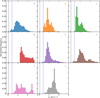 |
Fig. 9 Histogram of observed velocity dispersions of the eight cloud structures derived from the Effelsberg H2CO data. The vertical dashed black and blue lines represent the thermal velocity dispersion of H2CO and twice the sonic speed of 0.19 km s−1 at a kinetic temperature of 10 K, respectively. |
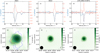 |
Fig. 10 H2CO spectra and their spatial distribution atan angular resolution of 25″. Top: observed H2CO (11,0−11,1) spectra of DR2l (a), DR22 (c), and G76.1883+0.0973 (e) overlaid on the fit results indicated by the dashed brown lines. The derived optical depth spectra are shown by the red lines. In panels a, c, e, the dashed vertical black lines represent the LSR velocities of the HII regions obtained from the radio recombination line measurements (Khan et al. in prep.). Bottom: VLA+Effelsberg 4.9 GHz radio continuum emission of DR2l (b), DR22 (d), and G76.1883+0.0973 (ƒ) overlaid with the H2CO (11,0−11,1) absorption contours. For DR2l, the blue and red contours represent the H2CO (11,0−11,0) absorption peak for the −3 km s−1 and 8 km s−1 components, respectively. The contours start at −0.1 Jy beam−1 (5σ), with each subsequent contour being twice the previous one. For DR22 and G76.1883+0.0973, the contours start at −0.1 Jy beam−1 (5σ) and decrease by 0.04 Jy beam−1. The synthesized beam is shown in the lower left corner of each panel. All the continuum and spectral line data are from the combination of the VLA D configuration and the Effelsberg single-dish observations. |
5.3 Nondetections
Although our Effelsberg observations also cover the  (11,0−11,1) line, the line is not detected in the Cygnus X region. At the HPBW of 3′ and the channel width of 2.5 km s−1, the 1er noise levels range from 0.02 K to 0.14 K with a median value of 0.06 K. Based on Eq. (1), we obtained a 3cr upper limit of 0.18 K at the position of the peak continuum emission position (Tc = 29.7 K, i.e., DR2l), which corresponds to an upper limit of 0.006 for the optical depth. Previous observations have detected
  (11,0−11,1) absorption toward DR2l (Wilson et al. 1976; Henkel et al. 1980; Yan et al. 2019), but with intensities that correspond to signals that are below our detection limit.
H2CO (11,0−11,1) masers are known to be associated with massive star formation in our Galaxy (e.g., Araya et al. 2004), but these masers have only been detected in 11 massive star-forming regions of the Milky Way to date (Forster et al. 1980; Whiteoak & Gardner 1983; Pratap et al. 1994; Araya et al. 2004, 2007, 2008; Ginsburg et al. 2015b; Chen et al. 2017; Lu et al. 2019; McCarthy et al. 2022). With both our Effelsberg 100 m and VLA observations, we did not detect any H2CO maser in Cygnus X. The 3σ upper limits for the masers are ~0.09–0.3 Jy at a channel width of 0.19 km s−1 for the Effelsberg observations and ~0.07 Jy at a channel width of 0.25 km s−1 for the VLA D-configuration observations.
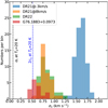 |
Fig. 11 Histogram of the observed velocity dispersions derived from the VLA+Effelsberg combined H2CO data. The vertical dashed black and blue lines represent the thermal velocity dispersion of H2CO and twice the sonic speed at a kinetic temperature of 20 K, respectively. |
6 Discussion
6.1 Absorbed photons on different scales
As mentioned in Sect. 2, the H2CO (11,0–11,1) line can be seen in absorption both against radio continuum sources and the CMB. Given the extent of bright radio continuum emission in Cygnus X, it is not well known which source plays the dominant role as a background for absorption on different scales. In order to address this question, we investigated the relation between the peak intensities of H2CO absorption and the brightness temperatures of the 4.9 GHz radio continuum emission.
For our GLOSTAR VLA+Effelsberg results on a scale of ~0.17 pc, all the detected absorption features are against bright continuum sources with brightness temperatures > 20 K (see Sect. 5.2), suggesting that they are caused by absorption of photons mainly from the HII regions rather than the CMB. At the sensitivity limit of our observations, we cannot estimate the relative importance of radio continuum and the CMB for weak absorption features on this scale.
We further carried out a pixel-by-pixel comparison between the peak intensities of H2CO absorption and the brightness temperatures of the 4.9 GHz radio continuum emission of the Effelsberg data, in which only the peak intensities of H2CO absorption with at least 5σ were taken into account. The results for two large scales (3′ and 10.′8, i.e., 1.2 pc and 4.4 pc) are shown in Fig. 12. As mentioned above, Fig. 12a is more strongly dominated by compact sources at the high-intensity end, and the points in the diagonal line arise from DR21. In contrast, Fig. 12b shows the relation for the extended H2CO absorption features. In both panels, a significant fraction of the Galactic 4.9 GHz continuum emission has brightness temperatures that are lower than the CMB (2.73 K; e.g., Fixsen 2009). Especially for the extended H2CO absorption (see Fig. 12b), about 97% of points have Galactic 4.9 GHz radio continuum emission brightness temperatures <2.73 K. We also find that 9.1% and 0.6% of the H2CO absorption dips can be greater than the Galactic radio continuum temperature in Fig. 5c at the 1σ and 3σ significance levels, respectively. Extreme cases like this are seen at around l = 77.877°, b = 0.865°. This unambiguously attributes the absorption primarily to the CMB. Overall, we expect that absorption of CMB photons contributes to extended H2CO absorption features in addition to radio continuum emission.
6.2 Formaldehyde abundance
Based on the derived total column density of ortho-H2CO (see Sect. 5.1.2 and Appendix A), we can estimate its molecular fractional abundance with respect to H2. Assuming, as usual, that the dust emission traces the H2 column density (Goodman et al. 2009), we used the Planck 353 GHz map of the dust optical depth (Planck Collaboration XI2014) and the HI column density map from the Effelsberg-Bonn HI survey (EHBIS; Winkel et al. 2016) to estimate the H2 column densities in this study. The dust optical depth at 353 GHz, τ353 consists of contributions from both molecular (H2) and atomic gas (HI). The column density of atomic gas, NHI, is related to τ353 by NHI = 8.3 × 1025τ353 cm−2 (Planck Collaboration XI 2014). Comparing the EHBIS HI column densities and the τ353-based HI column densities, we find that HI contributes to at least 26% of the dust-based HI column densities for pixels with the detection of H2CO absorption. Thus, the HI column density needs to be subtracted from the dust-based HI column density to calculate the H2 column density, which is determined as  , where NHI is based on the EBHIS HI column density map. All images were convolved to 10.′8 to calculate the H2 column densities and the ortho-H2CO fractional abundance.
Figure 13a presents a comparison between the derived H2 column densities and the ortho-H2CO column densities. It is expected that the ortho-H2CO column density increases with increasing H2 column density, and the Pearson correlation coefficient is 0.49. The molecular fractional abundances are found to range from 1.4×10⁻¹⁰ to 1.6×10⁻⁹ with a median value of 6.9×10⁻¹⁰ on a scale of 4.4 pc. On the other hand, the fractional abundances of ortho-H2CO appear to be unaffected by the H2 column densities on this scale because the Pearson correlation coefficient between the ortho-H2CO fractional abundances and the H2 column densities is only −0.17.
As shown in Fig. 13b, the histogram of the ortho-H2CO abundances displays a Gaussian-like behavior in the logarithmic space. We performed a Gaussian fit to the histogram, which resulted in a mean abundance of 7.0×10⁻¹⁰ with a dispersion of 0.15 dex (i.e., 10−9.16±0.15). Our values are roughly consistent with the ortho-H2CO abundances in the Galactic center and the W51 complex (Guesten & Henkel 1983; Ginsburg et al. 2015a). This suggests that the abundances do not vary significantly for the different environments on the cloud scale. This also agrees with previous para-H2CO studies that the fractional abundance of H2CO is rather stable and the variation is usually within an order of magnitude in different environments (e.g., Gerner et al. 2014; Zhu et al. 2020; Tang et al. 2021).
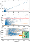 |
Fig. 12 Comparison between the peak intensities of H2CO absorption and the temperatures of the 4.89 GHz radio continuum emission at an angular resolution of 3′ (a) and 10.8 (b). All data points have signal-to-noise ratios of >5. In both panels, the dashed red line represents the CMB temperature of 2.73 K. (c) Same as panel a, but zoomed into a narrower intensity range. The panel in the lower right corner is the same as Fig. 5a, but zoomed into the region where the absorption dip is greater than the radio continuum temperature. In panels b and c, the dashed orange line marks the equality between H2CO peak absorption and radio continuum temperature. In all panels, the error bars represent the 1σ uncertainty. |
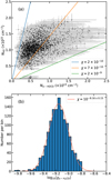 |
Fig. 13 Analysis of ortho-H2CO Abundances. (α) H2 column density as a function of the ortho-H2CO column density. The three lines represent the fractional abundances of 2 × 10⁻¹⁰, 7 × 10⁻¹⁰, and 2 × 10⁻⁹. (b) Statistic histogram of the ortho-H2CO abundance. The red line represents the Gaussian fit to the histogram. |
6.3 Comparison with other tracers
In order to compare the distribution of H2CO with that of other tracers including the 353 GHz dust optical depth, HI column density, and the 13CO (1–0) line, we used the integrated optical depth maps rather than the integrated-intensity map because the column density of H2CO is directly related to the optical depth. The different data sets were convolved to a common angular resolution of 10.′8 and projected onto the same grid as the H2CO absorption. Figure 14 shows the comparison between the distribution of different tracers at the same angular resolution of 10.8.
We used the structural similarity index (SSI10) to quantify the similarity between the distributions of different tracers (Wang et al. 2004). The SSI has a value between −1 and 1, where an SSI of 1 implies perfect similarity, an SSI of 0 implies no similarity, and an SSI of −1 implies a perfect anticorrelation. Before making this comparison, we performed the quantile transformer of our data to ensure that the pixel values followed the Gaussian distribution. The SSI was then estimated for different pairs of tracers. The comparison between H2CO and 13CO (1−0) results in an SSI of 0.38, which is higher than what was found for the other two pairs (the SSI for each pair is shown in the lower left corner in Fig. 14). The results show that the best overall morphological agreement is between H2CO (11,0−11,1) and 13CO (1−0). In contrast, the distribution of τ353 is more extended, while that of NHI is even more extended and often uncorrelated with both H2CO (11,0-11,1) and 13CO (1−0). This strongly suggests that our Effelsberg data of the H2CO (11,0−11,1) absorption trace the bulk of molecular gas, also seen in 13CO (1−0) emission (their relation is further investigated in Appendix D).
Previous observations have suggested that H2CO can exist in diffuse and translucent molecular clouds (e.g., Nash 1990; Liszt & Lucas 1995; Menten & Reid 1996; Snow & McCall 2006; Liszt et al. 2006). Hence, H2CO (11,0−11,1) can potentially be used to investigate the so-called CO-dark molecular gas (e.g., Grenier et al. 2005; Wolfire et al. 2010). However, our survey data appear to only trace molecular gas seen in 13CO (1−0). Previous observations suggested that the CO-dark molecular gas is prevalent over the visual extinction range 0.4 ≲ AV ≲ 2.5 (Planck Collaboration XIX 2011), while numerical simulations indicate that the CO-dark molecular gas can be present in gas with AV ≲ 5 (Seifried et al. 2020a). Given our sensitivity, our H2CO (11,0−11,1) observations can only probe molecular gas with H2 column densities ≳ 5 × 1021 cm−2 (i.e., AV ≳ 5) in Cygnus X (see Fig. 13). We also stacked the H2CO spectra for regions in which the 13CO (1−0) integrated intensities are lower than 0.15 K km s−1 (3σ), but H2CO absorption is not detected in the stacked spectrum. Therefore, we conclude that our observations do not reach the regime of the CO-dark molecular gas, and more sensitive observations are needed to address whether H2CO (11,0−11,1) can trace the CO-dark molecular gas.
6.4 Local velocity gradient
The distribution of velocity centroids seems to show ordered LSR velocity gradients rather than random motions. To study the LSR velocity gradients within the individual cloud structures, we followed the definition of the local velocity gradients, ∇υ, given by Goodman et al. (1993),
 (7)
(7)
where vlsr is the observed velocity centroid, υ0 is the systemic velocity centroid, ∆l and ∆b are the offsets in the Galactic longitude and latitude, and x and y are the components of ∇υ in the directions of the Galactic longitude and latitude. The magnitude of the local velocity gradient is defined as  . The position angle is θvg = arctan(x/y) and θ increases counterclockwise with respect to the Galactic northern direction. In order to derive the Vυ distribution, we fit Eq. (7) using the Levenberg-Marquardt algorithm toward each block of 3 × 3 pixels (e.g., Gong et al. 2021).
Figure 15 shows the derived ∇υ distribution of cloud E, and the results for the other cloud structures are presented in Fig. E.1. The magnitude |∇υ| lies in the range from 0 to 2.38 km s−1 pc−1 with a median value of 0.14 km s−1 pc−1. More than 80% of the |∇υ| values are lower than 0.3 km s−1 pc−1. The high |∇υ| values mainly arise from two cloud structures (clouds A and H) close to DR21 (see also Fig. E.1). The velocity gradients toward DR21 are thought to be caused by cloud-cloud collisions (Dickel et al. 1978). Furthermore, these plots confirm the presence of anisotropic velocity fields at least in parts of clouds on the large scale of 4.4 pc.
Because gravity and turbulence can also affect the relative orientations between local velocity gradients and magnetic fields, we used the alignment measure (AM) to further investigate their relation. Following previous studies (e.g., Lazarian & Yuen 2018; Liu et al. 2023), AM is defined as
 (8)
(8)
where ϕ is the relative orientation between the local velocity gradients and the magnetic fields in the range of 0º–90º. AM has a value between −1 and 1, where AM = −1 implies perpendicular and AM = 1 implies parallel alignment.
Figure 16 presents AM as a function of velocity dispersion and H2 column density on the 4.4 pc scale. In Fig. 16a, AM appears to be uncorrelated with velocity dispersion. This is different from the previous study of the Taurus cloud, where strongly parallel or perpendicular alignments were restricted to regions with low levels of turbulence (Heyer et al. 2020). This is because Cygnus X is more turbulent than the Taurus cloud and the correlation is weak in case of strong turbulence (González-Casanova & Lazarian 2017; Lazarian & Yuen 2018).
Figure 16b shows that AM tends to be more parallel at high H2 column densities of ≳1.8 × 1022 cm−2. In high-density regions, in which gravity becomes dominant, molecular gas tends to flow along magnetic field lines because of the resisting Lorentz force in the perpendicular direction (e.g., Li et al. 2014). Our observations thus support that gas motions are channeled by gravity and magnetic fields in Cygnus X when the H2 column densities are ≳ 1.8 × 1022 cm−2 on the 4.4 pc scale. The critical H2 column density for the transition from being perpendicular to being parallel appears to be higher than the values (1021–21.5 cm−2) predicted by previous simulations (Seifried et al. 2020b). However, the plane-of-sky magnetic field strengths in the ambient gas surrounding DR21 have been estimated to be ~0.1 mG (Ching et al. 2022), which is much higher than the values (≲10 µG) adopted in the simulations (Seifried et al. 2020b). The critical H2 column density should depend on the magnetic field strength (e.g., Li et al. 2014; Seifried et al. 2020b). Therefore, the higher critical H2 column density in Cygnus X can be explained by its stronger magnetic fields.
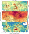 |
Fig. 14 Comparison between the H2CO distribution with that of τ353, NHI, and 13CO. The spatial distribution of τ353 is derived from the Planck measurements (top), the HI column density from EBHIS (Winkel et al. 2016), and the13 CO (1−0) integrated intensity from Schneider et al. (2011) at an angular resolution of 10.8. In all panels, the contours correspond to the smoothed integrated optical depth map of H2CO (11,0−11,1) integrated from −10 km s−1 to 20 km s−1, and they start from 0.09 km s−1 and increase by 0.09 km s−1. The SSI (see Sect. 6.3) of the two corresponding tracers is indicated in the lower left corner of each panel. |
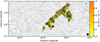 |
Fig. 15 Local velocity gradient map overlaid with the magnetic field pattern derived from the Planck 353 GHz dust polarization. The arrows represent the direction of normalized local velocity gradients, and the color bar represents the magnitude of the local velocity gradients in units of km s−1 pc−1. The beam size is shown in the lower right corner. The coherent structure is labeled in the top right corner. |
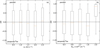 |
Fig. 16 Alignment measure as a function of velocity dispersion (panel a) and H2 column density (panel b). In each box plot, the median value is indicated by an orange line, and the box represents the data within the 25th and 75th percentiles. |
6.5 Comparison of multiscale motions
Molecular clouds are known to show hierarchical structures (e.g., Rosolowsky et al. 2008). However, the connection between the large- and smal-lscale structures is not well established. Our Effelsberg and VLA observations allowed us to study the relation between the large- and small-scale properties.
Because H2CO absorption is only detected toward three bright HII regions (i.e., DR21, DR22, and G76.1883+0.0973) by our high angular resolution observations, we can only meaningfully compare the gas properties toward these regions on different scales. Figure 17 shows the comparison of the derived velocity dispersions on different scales. According to the classical turbulence cascade theory (e.g., Elmegreen & Scalo 2004; Scalo & Elmegreen 2004) and previous observational studies (e.g., Larson 1981; Qian et al. 2012; Schuller et al. 2017), gas motions should decrease toward small scales. Our observations agree with this scenario, except for the −3 km s−1 component of DR21, which has nearly identical velocity dispersions on different scales (0.17−4.4 pc). This contradicts the expected behavior of this classic turbulence, which is thought to be externally driven on large scales of ≳10 pc, with turbulent energy cascading down to small scales (e.g., Elmegreen & Scalo 2004; Scalo & Elmegreen 2004).
In order to explain this behavior, we speculate that the fact that we find nearly identical velocity dispersions on different scales indicates that the turbulence in the DR21 region is driven on scales <4.4 pc. Previous studies have proposed cloud-cloud collisions between the −3 km s−1 and 8 km s−1 components of DR21 (Dickel et al. 1978; Dobashi et al. 2019), which can drive the additional turbulence. If the small-scale turbulence is due to a cloud-cloud collision, we expect to see an enhancement of turbulent motions in both velocity components. However, the 8 km s−1 component seems to follow the turbulence cascade picture (see Fig. 17). Instead, the additional turbulence in the −3 km s−1 component can be induced by locally convergent flows that result from self-gravity (Schneider et al. 2010). Theoretical studies also suggested that the shallower relation between velocity dispersion and linear scales is indicative of gravitational collapse (e.g., Murray & Chang 2015; Vázquez-Semadeni et al. 2019). Alternatively, the additional turbulence can be driven by the powerful protostellar outflow in the region. DR21 is known to host one of the most powerful outflows in Cygnus X, whose lobes extend over ~1.6 pc (Garden & Carlstrom 1992; Skretas et al., in prep.). Because the −3 km s−1 component of DR21 is physically associated with the molecular outflow, the outflow-driven turbulence can affect nearly all the physical scales probed in Fig. 17. While molecular outflows may also exist close to DR22 and G76.1883+0.0973 (e.g., Shepherd & Churchwell 1996; Skretas & Kristensen 2022), they may be too weak to drive additional turbulence comparable to that toward DR21. Another possible source of turbulence could come from the associated HII regions. As shown in Sect. 5.2, the comparison between the RRL and H2CO velocity suggests that the −3 km s−1 component of DR21 is likely the only molecular gas that is associated with HII regions. Hence, the feedback of HII regions could also lead to the difference behavior of the −3 km s−1 component of DR21. Therefore, we suggest that the nearly identical velocity dispersions toward the −3 km s−1 component of DR21 on different scales can be caused by internally driven turbulence from convergent flows, YSO outflows, and H11 regions.
We also note that our H2CO absorption measurements probe all of the gas along the line of sight. The probed lengths along the line of sight are completely unknown, which could bias the representative scales in Fig. 17.
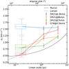 |
Fig. 17 Velocity dispersions of H2CO (11,0−11,1) as a function of different linear scales toward the targeted sources. The classic Larson relation is indicated by the dotted black line (Larson 1981), and the relation between the velocity dispersion and linear scales in the Taurus molecular cloud is shown by the dashed black line (Qian et al. 2012). |
7 Summary and conclusion
As part of the GLOSTAR survey project, we carried out Effelsberg and VLA observations toward the Cygnus X region to study the multiscale structure properties of its molecular gas. The main findings are summarized as follows:
Our Effelsberg observations reveal widespread H2CO (11,0 − 11,1) absorption with a typical spatial extent of ≳50 pc in Cygnus X. Most of the observed H2CO absorption is optically thin. Based on a decomposition of the spectra to a scale of 4.4 pc and the DBSCAN clustering method, we assign the observed H2CO absorption into eight velocity-coherent cloud structures that are dominated by supersonic turbulent motions;
The GLOSTAR VLA+Effelsberg combined data result in the robust detection of H2CO (11,0 − 11,1) absorption toward three HII regions (i.e., DR21, DR22, and G76.1883+0.0973). The observed velocity dispersions suggest that supersonic turbulence commonly exists in the three HII regions on the 0.17 pc scale;
While the compact absorption features are mainly due to absorption against the radio continuum in Cygnus X, extended absorption features are also seen where the radio continuum is weak. This suggests a non-negligible contribution of the CMB in producing extended absorption features in Cygnus X;
On a large scale, our comparison of different tracers shows a high degree of similarity in the distributions of the H2CO (11,0 − 11,1) absorption and 13CO (1−0) emission, indicating that H2CO (11,0 − 11,1) can trace the bulk of the molecular gas seen in 13CO (1−0). Making use of the Planck 353 GHz dust optical depth map, HI column density map, and our H2CO observations, we find that H2CO (11,0 − 11,1) can trace molecular gas with H2 column densities of ≳ 5 × 1021 cm−2 (i.e., AV ≳ 5) and the ortho-H2CO fractional abundances with respect to H2 has a mean abundance of 7.0×10⁻¹⁰, with a dispersion of 0.15 dex (i.e., 10−916±015);
Local velocity gradients were investigated on scales of 4.4 pc and 0.17 pc. On the 4.4 pc scale, most of the magnitudes of the local velocity gradients are as low as <0.3 km s−1 pc−1. We find that the relative orientation between local velocity gradient and magnetic field tends to be more parallel at H2 column densities of >1.8×1022 cm−2, which could be caused by a scenario in which gas motions are channeled by magnetic fields;
Multiscale comparisons of velocity dispersions show that the −3 km s−1 component of DR21 has nearly identical velocity dispersions on scales of 0.17–4.4 pc, which might deviate from the expected behavior of classic turbulence. This could be caused by internally driven turbulence from convergent flows, YSO outflows, and HII regions.
Our GLOSTAR observations reveal widespread H2CO (11,0 – 11,1) absorption and pinpoint the bright absorption regions in Cygnus X, demonstrating that the GLOSTAR data can probe the H2CO (11,0 − 11,1) absorption on cloud (≳4 pc) down to core scales (~0.17 pc). Follow-up H2CO (21,1 − 21,2) observations of regions showing appreciable H2CO (11,0 – 11,1) absorption will allow for determinations of the density distributions of the covered molecular clouds.
Interactive Figures
Interactive 3D images associated with Fig. 7 (cyg-h2co-amp and cyg-h2co-dis) Access here
Acknowledgements
We thank the Effelsberg-100 m telescope staff for their assistance with our observations. H.B. acknowledges support from the European Research Council under the Horizon 2020 Framework Programme via the ERC Consolidator Grant CSF-648505. H.B. also acknowledges support from the Deutsche Forschungsgemeinschaft in the Collaborative Research Center (SFB 881) “The Milky Way System” (subproject B1). A.Y.Y. acknowledges support from the NSFC grants No. 11988101 and No. NSFC 11973013. We thank Nicola Schneider for sharing her FCRAO data cubes. Y.G. thanks Xuyang Gao for helpful discussions on the zero level restoration of the continuum data in Cygnus X. Y.G. thanks Tao-Chung Ching for sharing the JCMT POL-2 data on DR21. This work is based on observations with the 100-m telescope of the MPIfR (Max-Planck-Institut für Radioastronomie) at Effelsberg. The National Radio Astronomy Observatory is a facility of the National Science Foundation operated under cooperative agreement by Associated Universities, Inc. This research has made use of NASA’s Astrophysics Data System. This work also made use of Python libraries including Astropy (https://www.astropy.org/; Astropy Collaboration 2013), NumPy (https://www.numpy.org/; van der Walt et al. 2011), SciPy (https://www.scipy.org/; Jones et al. 2001), Matplotlib (https://matplotlib.org/; Hunter 2007), LMFIT (Newville et al. 2014), APLpy (Robitaille & Bressert 2012), plotly (https://plotly.com/), and magnetar (https://github.com/solerjuan/magnetar; Soler et al. 2013). We would like to thank the anonymous referee for the valuable comments which improve our draft. S.A.D. acknowledges the M2FINDERS project from the European Research Council (ERC) under the European Union s Horizon 2020 research and innovation programme (grant No 101018682).
Appendix A Total formaldehyde column density
Because of an unusual collisional pumping process, the level populations of ortho-H2CO corresponding to the 11,0−11,1 transition often deviate from what is expected under conditions of local thermodynamic equilibrium (LTE). Hence, we did not derive the total ortho-H2CO column density from observations of this single line under the assumption of LTE. Instead, we used the following approach. First, we explored the level populations of ortho-H2CO for a range of physical conditions (that can be expected on scales > 4.4 pc) using a standard non-LTE radiative transfer model, and determined the fractional population at the 11,0 level. We then determined the total ortho H2CO column density by scaling the column density at the 11,0 level by a factor at fiducial values of the physical conditions in the Cygnus X region.
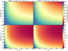 |
Fig. A.1 RADEX calculations of the fractional population at the 11,0 level (top panels) and excitation temperatures (bottom panels). The left and right panels correspond to the two different specific column densities of 1 × 1012 cm−2 (km s−1)−1 and 1 × 1013 cm−2 (km s−1)−1, respectively. |
In order to investigate the level populations of ortho-H2CO, we used the non-LTE RADEX11 code (van der Tak et al. 2007). The molecular data of ortho-H2CO were obtained from the Leiden Atomic and Molecular Database (LAMDA12; Schöier et al. 2005), where the energy levels, transition frequencies, and Einstein A coefficients are taken from the CDMS catalog (Müller et al. 2005; Endres et al. 2016) and the collisional rates are taken from Wiesenfeld & Faure (2013). A total of 40 energy levels were considered in our calculations. Based on the previous temperature measurements toward Cygnus X (Keown et al. 2019; Cao et al. 2019), most of the molecular gas lies in the kinetic temperature range of 10–30 K. Hence, we performed our calculations at kinetic temperatures ranging from 5 K to 30 K with a step size of 1 K. Because previous observations have shown H2 number densities of 500–5000 cm−3 on a scale of ≳0.3 pc (e.g., Nishimura et al. 2015), we expect that the H2 number density range of 102−104 cm−3 on a scale of 4.4 pc should be suitable for our cases. Therefore, the H2 number density, in units of cm−3, was varied logarithmically, with log[n(H2)] from 2 to 4 with a step size of 0.1. The ortho-to-para ratio of H2 was fixed to be 0.25 according to previous studies (e.g., Neufeld et al. 2006). For the specific column density (defined as the ratio of the column density and line width), we adopted a range from 1 × 1012 cm−2 (km s−1)−1 to 1 × 1013 cm−2 (km s−1)−1.
Figures A.1a–A.1b present the modeling results of the fractional population at the 11,0 level. The modeling results suggest that the population at the 11,0 level accounts for 34.2%–41.9% of the total population within the specific column density range of 1 × 1012 cm−2−1 × 1013 cm−2 (km s−1)−1. This shows that the fractional population does not change significantly for the range of physical conditions expected in Cygnus X. Furthermore, the modeling results show that the excitation temperatures range from 0.7 to 2.3 K (see Fig. A.1c–A.1d), which suggests that an excitation temperature of 1.6 K (see Sect. 5.1.2) is a reasonable assumption.
To determine the total H2CO column density, we adopted a kinetic temperature of 10 K, and H2 density of 103 cm−3 and a specific H2CO column density of 5×1012 cm−2 (km s−1)−1 as fiducial physical conditions in Cygnus X on a scale of ~4.4 pc. For these parameters, the fractional column density of H2CO at the 11,0 level is ≈ 0.39. With this ratio and using Eq. 3, the total ortho H2CO column density can be simply estimated by scaling the integrated optical depths of the H2CO (11,0–11,1) line,
 (A.1)
(A.1)
We also note that adopting a constant ratio of 39% implies an additional ~ 13% uncertainty in the derived column densities at most. We conclude that Eq. (A.1) can provide a reasonable estimate of the total ortho-H2CO column density when only the single transition H2CO (11,0−11,1) is observed.
Appendix B Overlap effects of the hyperfine structure lines of H2CO (11,0−11,1)
The H2CO (11,0−11,1) transition is known to have six HFS lines (e.g., Tucker et al. 1971), which overlap on account of line broadening. This can bias the measurements of the line widths and velocity centroids. In order to study the overlap effects of the HFS lines of H2CO (11,0−11,1), we followed the method introduced in Appendix D of Gong et al. (2021). We specified the rest frequencies and relative line strengths of the six HFS lines based on the CDMS (Müller et al. 2005). For the fiducial case, we assumed an excitation temperature, Tex, of 1.6 K, the microwave background radiation temperature, Tbg, to be 2.73 K, that no continuum emission arises from behind the H2CO-bearing gas (i.e., Tc =0 K), and the systemic LSR velocity, υ0, to be 0 km s−1. These parameters do not affect the velocity information of synthetic spectral line profiles, but only affect the amplitude of synthetic spectra. The peak optical depths can vary within the range of 0–0.5 (see Fig. 6). We used different peak optical depths, τ0, and velocity dispersion, σ0, to create synthetic spectra to test the overlapping effects.
Figure B.1 presents two synthetic spectra for different values of the velocity dispersion. It is evident that the absorption intensity still peaks at υlsr ~0 km s−1 for a low-velocity dispersion (see Fig. B.1a), but shifts to the blueshifted side at a higher velocity dispersion (see Fig. B.1b). For high-velocity dispersions, the F=1−0 line can create a redshifted wing-like profile that should not be misinterpreted as an indication of molecular outflows (see Fig. B.1b).
We also note that these profiles deviate from the typical Gaussian profile. Especially when the synthetic spectral line profiles are fit with the Gaussian function to derive the observed parameters, the derived velocity centroids and line widths can deviate from their true values. In order to understand this effect, we adopted different velocity dispersions from 0.1 km s−1 to 1 km s−1 with a step of 0.1 km s−1 and different peak optical depths from 0.1 to 1 with a step of 0.1. The deviation is characterised by the velocity difference, υG − υ0, and the ratio of the velocity dispersions, σG/σ0, where υG and σG are the fit velocity centroid and dispersion obtained from Gaussian fitting. In order to reduce the broadening effects caused by the F =1−0 line (see Fig. B.1), we only performed the Gaussian fit to the spectra within the velocity range from −2 km s−1 to 1 km s−1. The results are shown in Fig. B.2. The results demonstrate that both υG − υ0 and σG/σ0 are largely regulated by velocity dispersions. When σ0=0.3–0.4 km s−1, υG – υ0 can be as high as –0.1 km s−1. On the other hand, σG/σ0 increases with decreasing σ0, with the highest ratio of >2 at σ0=0.1 km s−1. Therefore, these overlapping effects should not be neglected in studying the kinematics with this transition.
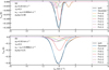 |
Fig. B.1 Synthetic H2CO (11,0−11,1) spectra (solid black lines) with the modeled τ0 and συ shown in the upper left corners. The Gaussian fitting results are indicated by the solid blue lines. The different HFS components are indicated by the colored dashed lines in the legend. |
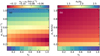 |
Fig. B.2 Effects of line profiles deviating from a typically Gaussian shape. (a) υG − υ0 as a function of optical depth and velocity dispersion, where υG and υ0 are the velocity centroid derived from the Gaussian fitting and the intrinsic velocity centroid. (b) σG/σ0 as a function of optical depth and velocity dispersion, where σG and σ0 are the velocity dispersion derived from the Gaussian fitting and the intrinsic velocity dispersion. |
We also note that H2CO (11,0–11,1) is typically not in LTE, which can cause the line ratios of HFS lines to be different from what is expected under LTE. However, the available collisional rate coefficients do not include the HFS lines (Wiesenfeld & Faure 2013), and non-LTE effects for the HFS lines are beyond the scope of this work.
Appendix C Parameterizing DBSCAN
Because the clustering results of the DBSCAN algorithm depend on e, we studied the influences of the varied e on the clustering results here. We ran the algorithm with different values of e to investigate the clustering results. As in Sect. 5.1.3, we discarded clustering structures with areas of less than three beams (10′.8). The results are presented in Fig. C.1. Comparing the results, we find that the clustering method tends to result in more extended structure with higher e. Usually, higher silhouette scores indicate better results. The silhouette scores converge to 0.37 for ϵ ≳1.25 when only one cloud structure is identified. Because the clustering results are mainly used to separate the line-of-sight velocity components to derive the local velocity gradients (see Sect. 6.4), the clustering results of the high e values are not suitable for our cases. Hence, we selected the clustering results manually based on Fig. C.1. A few large structures are missing in the clustering results with ϵ ≤0.18, while many discrete and small structures with areas of less than three beams emerge for ϵ ≥0.50. Furthermore, the line-of-sight overlapped velocity structures around l =81.5°, b=0.3° are well separated by ϵ =0.25, but not by ϵ =0.5. In order to study the velocity fields of extended structures, we chose ϵ=0.25 for our study. The local velocity gradients are exactly the same for the same pixels in the different clustering results, except for boundary pixels, which only make negligible difference in the velocity gradient maps. On the other hand, the most affected results are the cloud areas, but the cloud areas are not used to reach any conclusion. Therefore, we conclude that our results with ϵ =0.25 in this work should be valid.
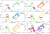 |
Fig. C.1 Cloud structures identified by the DBSCAN algorithm with different e values. The e value and silhouette score are indicated in the upper right corner of each panel. The different structures are marked with different colors. |
Appendix D Relation between H2CO (11,0—11,1) and 13CO(1−0)
The relation between H2CO and CO isotopologs has been investigated by previous studies (e.g., Tang et al. 2013, 2014). Our observations enable the comparison with a much larger sample size. Figure D.1 presents a comparison between the integrated properties of 13CO (1−0) and H2CO (1ı,o−11,1)· This comparison shows that the correlation coefficient (0.45) between 13CO (1−0) and H2CO (11,0-11,1) integrated intensities is lower than the correlation coefficient (0.51) between 13CO (1−0) integrated intensities and the integrated optical depth of H2CO (11,0-11,1)· Furthermore, Figure D.1 a appears to show a higher degree of scattering than Figure D.1b. Because the optical depths are derived by assuming that all radio continuum emission is located behind the molecular clouds, we speculate that most of the molecular gas should lie in front of the radio continuum emission. This is further supported by optical images, in which molecular clouds are seen as dark patches in Cygnus X (see Fig. 1 in Schneider et al. 2006 for instance).
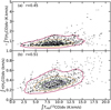 |
Fig. D.1 13CO (1−0) integrated intensities as a function of the absolute values of the H2CO integrated intensities (a) and the integrated optical depths of H2CO (b). |
Appendix E Local velocity gradient maps
The local velocity gradient map for cloud E has been presented in Sect. 5.1.3, and the local velocity gradient maps of the remaining seven clouds are shown in Fig. E.1.
References
- Abeysekara, A. U., Albert, A., Alfaro, R., et al. 2021, Nat. Astron., 5, 465 [NASA ADS] [CrossRef] [Google Scholar]
- Anderson, L. D., Bania, T. M., Balser, D. S., et al. 2014, ApJS, 212, 1 [Google Scholar]
- Ao, Y., Henkel, C., Menten, K. M., et al. 2013, A & A, 550, A135 [NASA ADS] [CrossRef] [EDP Sciences] [Google Scholar]
- Araya, E., Hofner, P., Linz, H., et al. 2004, ApJS, 154, 579 [NASA ADS] [CrossRef] [Google Scholar]
- Araya, E., Hofner, P., Goss, W. M., et al. 2007, ApJS, 170, 152 [NASA ADS] [CrossRef] [Google Scholar]
- Araya, E. D., Hofner, P., Goss, W. M., et al. 2008, ApJS, 178, 330 [NASA ADS] [CrossRef] [Google Scholar]
- Astropy Collaboration (Robitaille, T. P., et al.) 2013, A & A, 558, A33 [NASA ADS] [CrossRef] [EDP Sciences] [Google Scholar]
- Bennett, C. L., Larson, D., Weiland, J. L., et al. 2013, ApJS, 208, 20 [Google Scholar]
- Berlanas, S. R., Herrero, A., Comerón, F., et al. 2018, A & A, 612, A50 [NASA ADS] [CrossRef] [EDP Sciences] [Google Scholar]
- Beuther, H., Wyrowski, F., Menten, K. M., et al. 2022, A & A, 665, A63 [NASA ADS] [CrossRef] [EDP Sciences] [Google Scholar]
- Bieging, J. H., Wilson, T. L., & Downes, D. 1982, A & AS, 49, 607 [NASA ADS] [Google Scholar]
- Bonne, L., Bontemps, S., Schneider, N., et al. 2023, ApJ, 951, 39 [CrossRef] [Google Scholar]
- Bontemps, S., Motte, F., Csengeri, T., & Schneider, N. 2010, A & A, 524, A18 [NASA ADS] [CrossRef] [EDP Sciences] [Google Scholar]
- Brunthaler, A., Menten, K. M., Dzib, S. A., et al. 2021, A & A, 651, A85 [NASA ADS] [CrossRef] [EDP Sciences] [Google Scholar]
- Cabral, B., & Leedom, L. C. 1993, in Proceedings of the 20th Annual Conference on Computer Graphics and Interactive Techniques, SIGGRAPH ’93 (New York, NY, USA: Association for Computing Machinery), 263 [CrossRef] [Google Scholar]
- Cao, Y., Qiu, K., Zhang, Q., et al. 2019, ApJS, 241, 1 [Google Scholar]
- Cao, Y., Qiu, K., Zhang, Q., Wang, Y., & Xiao, Y. 2021a, ApJ, 918, L4 [NASA ADS] [CrossRef] [Google Scholar]
- Cao, Z., Aharonian, F. A., An, Q., et al. 2021b, Nature, 594, 33 [NASA ADS] [CrossRef] [Google Scholar]
- Cao, Y., Qiu, K., Zhang, Q., & Li, G.-X. 2022, ApJ, 927, 106 [NASA ADS] [CrossRef] [Google Scholar]
- Cash, W., Charles, P., Bowyer, S., et al. 1980, ApJ, 238, L71 [Google Scholar]
- Chen, X., Shen, Z.-Q., Ellingsen, S. P., et al. 2017, ApJ, 851, L3 [NASA ADS] [CrossRef] [Google Scholar]
- Chen, B. Q., Li, G. X., Yuan, H. B., et al. 2020, MNRAS, 493, 351 [NASA ADS] [CrossRef] [Google Scholar]
- Cheng, Y., Gutermuth, R. A., Offner, S., et al. 2022, MNRAS, 512, 960 [CrossRef] [Google Scholar]
- Ching, T.-C., Qiu, K., Li, D., et al. 2022, ApJ, 941, 122 [CrossRef] [Google Scholar]
- Cotton, W. D. 2008, PASP, 120, 439 [Google Scholar]
- Cyganowski, C. J., Reid, M. J., Fish, V. L., & Ho, P. T. P. 2003, ApJ, 596, 344 [Google Scholar]
- Deb, S., Kothes, R., & Rosolowsky, E. 2021, MNRAS, 503, 1264 [Google Scholar]
- Dharmawardena, T. E., Bailer-Jones, C. A. L., Fouesneau, M., & Foreman-Mackey, D. 2022, A & A, 658, A166 [NASA ADS] [CrossRef] [EDP Sciences] [Google Scholar]
- Dickel, J. R., Dickel, H. R., & Wilson, W. J. 1978, ApJ, 223, 840 [Google Scholar]
- Dobashi, K., Shimoikura, T., Katakura, S., Nakamura, F., & Shimajiri, Y. 2019, PASJ, 71, S12 [NASA ADS] [CrossRef] [Google Scholar]
- Dokara, R., Brunthaler, A., Menten, K. M., et al. 2021, A & A, 651, A86 [NASA ADS] [CrossRef] [EDP Sciences] [Google Scholar]
- Dokara, R., Gong, Y., Reich, W., et al. 2023, A & A, 671, A145 [NASA ADS] [CrossRef] [EDP Sciences] [Google Scholar]
- Duarte-Cabral, A., Bontemps, S., Motte, F., et al. 2013, A & A, 558, A125 [NASA ADS] [CrossRef] [EDP Sciences] [Google Scholar]
- Dzib, S. A., Rodríguez, L. F., Loinard, L., et al. 2013, ApJ, 763, 139 [Google Scholar]
- Dzib, S. A., Yang, A. Y., Urquhart, J. S., et al. 2023, A & A, 670, A9 [Google Scholar]
- Elmegreen, B. G., & Scalo, J. 2004, ARA & A, 42, 211 [NASA ADS] [CrossRef] [Google Scholar]
- Emig, K. L., White, G. J., Salas, P., et al. 2022, A & A, 664, A88 [NASA ADS] [CrossRef] [EDP Sciences] [Google Scholar]
- Endres, C. P., Schlemmer, S., Schilke, P., Stutzki, J., & Müller, H. S. 2016, J. Mol. Spectrosc., 327, 95 [NASA ADS] [CrossRef] [Google Scholar]
- Ester, M., Kriegel, H.-P., Sander, J., & Xu, X. 1996, in Proceedings of the Second International Conference on Knowledge Discovery and Data Mining, KDD’96 (AAAI Press), 226 [Google Scholar]
- Evans, N. J. I., Zuckerman, B., Morris, G., & Sato, T. 1975, ApJ, 196, 433 [NASA ADS] [CrossRef] [Google Scholar]
- Fabricant, B., Krieger, D., & Muenter, J. S. 1977, J. Chem. Phys., 67, 1576 [NASA ADS] [CrossRef] [Google Scholar]
- Fixsen, D. J. 2009, ApJ, 707, 916 [Google Scholar]
- Forster, J. R., Goss, W. M., Wilson, T. L., Downes, D., & Dickel, H. R. 1980, A & A, 84, L1 [NASA ADS] [Google Scholar]
- Garden, R. P., & Carlstrom, J. E. 1992, ApJ, 392, 602 [CrossRef] [Google Scholar]
- Gerner, T., Beuther, H., Semenov, D., et al. 2014, A & A, 563, A97 [NASA ADS] [CrossRef] [EDP Sciences] [Google Scholar]
- Ginsburg, A., Bally, J., Battersby, C., et al. 2015a, A & A, 573, A106 [CrossRef] [EDP Sciences] [Google Scholar]
- Ginsburg, A., Walsh, A., Henkel, C., et al. 2015b, A & A, 584, A7 [Google Scholar]
- Gong, Y., Belloche, A., Du, F. J., et al. 2021, A & A, 646, A170 [NASA ADS] [CrossRef] [EDP Sciences] [Google Scholar]
- González-Casanova, D. F., & Lazarían, A. 2017, ApJ, 835, 41 [CrossRef] [Google Scholar]
- Goodman, A. A., Benson, P. J., Fuller, G. A., & Myers, P. C. 1993, ApJ, 406, 528 [Google Scholar]
- Goodman, A. A., Pineda, J. E., & Schnee, S. L. 2009, ApJ, 692, 91 [Google Scholar]
- Gottschalk, M., Kothes, R., Matthews, H. E., Landecker, T. L., & Dent, W. R. F. 2012, A & A, 541, A79 [NASA ADS] [CrossRef] [EDP Sciences] [Google Scholar]
- Gregory, P. C., & Condon, J. J. 1991, ApJS, 75, 1011 [Google Scholar]
- Grenier, I. A., Casandjian, J.-M., & Terrier, R. 2005, Science, 307, 1292 [Google Scholar]
- Guesten, R., & Henkel, C. 1983, A & A, 125, 136 [NASA ADS] [Google Scholar]
- Heiles, C. 1973, ApJ, 183, 441 [NASA ADS] [CrossRef] [Google Scholar]
- Henkel, C., Walmsley, C. M., & Wilson, T. L. 1980, A & A, 82, 41 [NASA ADS] [Google Scholar]
- Henkel, C., Wilson, T. L., Walmsley, C. M., & Pauls, T. 1983, A & A, 127, 388 [NASA ADS] [Google Scholar]
- Hennemann, M., Motte, F., Schneider, N., et al. 2012, A & A, 543, A3 [Google Scholar]
- Heyer, M., Soler, J. D., & Burkhart, B. 2020, MNRAS, 496, 4546 [NASA ADS] [CrossRef] [Google Scholar]
- Hu, B., Qiu, K., Cao, Y., et al. 2021, ApJ, 908, 70 [NASA ADS] [CrossRef] [Google Scholar]
- Hunter, J. D. 2007, Comput. Sci. Eng., 9, 90 [NASA ADS] [CrossRef] [Google Scholar]
- Jones, E., Oliphant, T., Peterson, P., et al. 2001, SciPy: Open source scientific tools for Python [Google Scholar]
- Kauffmann, J., Bertoldi, F., Bourke, T. L., Evans, N. J. I., & Lee, C. W. 2008, A & A, 487, 993 [NASA ADS] [CrossRef] [EDP Sciences] [Google Scholar]
- Keown, J., Di Francesco, J., Rosolowsky, E., et al. 2019, ApJ, 884, 4 [Google Scholar]
- Kerp, J., Winkel, B., Ben Bekhti, N., Flöer, L., & Kalberla, P. M. W. 2011, Astron. Nachr., 332, 637 [NASA ADS] [CrossRef] [Google Scholar]
- Klein, B., Hochgürtel, S., Krämer, I., et al. 2012, A & A, 542, A3 [Google Scholar]
- Knödlseder, J. 2000, A & A, 360, 539 [Google Scholar]
- Komesh, T., Esimbek, J., Baan, W., et al. 2019, ApJ, 874, 172 [NASA ADS] [CrossRef] [Google Scholar]
- Kryukova, E., Megeath, S. T., Hora, J. L., et al. 2014, AJ, 148, 11 [Google Scholar]
- Kurtz, S., Churchwell, E., & Wood, D. O. S. 1994, ApJS, 91, 659 [Google Scholar]
- Larson, R. B. 1981, MNRAS, 194, 809 [Google Scholar]
- Lazarian, A., & Yuen, K. H. 2018, ApJ, 853, 96 [NASA ADS] [CrossRef] [Google Scholar]
- Li, H. B., Goodman, A., Sridharan, T. K., et al. 2014, in Protostars and Planets VI, eds. H. Beuther, R. S. Klessen, C. P. Dullemond, & T. Henning, 101 [Google Scholar]
- Li, C., Qiu, K., Hu, B., & Cao, Y. 2021a, ApJ, 918, L2 [NASA ADS] [CrossRef] [Google Scholar]
- Li, G.-X., Cao, Y., & Qiu, K. 2021b, ApJ, 916, 13 [NASA ADS] [CrossRef] [Google Scholar]
- Li, C., Qiu, K., Li, D., et al. 2023, ApJ, 948, L17 [CrossRef] [Google Scholar]
- Liszt, H., & Lucas, R. 1995, A & A, 299, 847 [NASA ADS] [Google Scholar]
- Liszt, H. S., Lucas, R., & Pety, J. 2006, A & A, 448, 253 [NASA ADS] [CrossRef] [EDP Sciences] [Google Scholar]
- Liu, J., Zhang, Q., Koch, P. M., et al. 2023, ApJ, 945, 160 [NASA ADS] [CrossRef] [Google Scholar]
- Lockman, F. J. 1989, ApJS, 71, 469 [Google Scholar]
- Lu, X., Mills, E. A. C., Ginsburg, A., et al. 2019, ApJS, 244, 35 [Google Scholar]
- Mangum, J. G., & Shirley, Y. L. 2015, PASP, 127, 266 [Google Scholar]
- Mangum, J. G., & Wootten, A. 1993, ApJS, 89, 123 [Google Scholar]
- Mangum, J. G., Darling, J., Menten, K. M., & Henkel, C. 2008, ApJ, 673, 832 [NASA ADS] [CrossRef] [Google Scholar]
- McCarthy, T. P., Orosz, G., Ellingsen, S. P., et al. 2022, MNRAS, 509, 1681 [Google Scholar]
- McMullin, J. P., Waters, B., Schiebel, D., Young, W., & Golap, K. 2007, ASP Conf. Ser., 376, 127 [Google Scholar]
- Medina, S. N. X., Urquhart, J. S., Dzib, S. A., et al. 2019, A & A, 627, A175 [NASA ADS] [CrossRef] [EDP Sciences] [Google Scholar]
- Menten, K. M., & Reid, M. J. 1996, ApJ, 465, L99 [NASA ADS] [CrossRef] [Google Scholar]
- Motte, F., Bontemps, S., Schilke, P., et al. 2007, A & A, 476, 1243 [NASA ADS] [CrossRef] [EDP Sciences] [Google Scholar]
- Müller, H. S. P., Schlöder, F., Stutzki, J., & Winnewisser, G. 2005, J. Mol. Struct., 742, 215 [Google Scholar]
- Müller, P., Krause, M., Beck, R., & Schmidt, P. 2017, A & A, 606, A41 [CrossRef] [EDP Sciences] [Google Scholar]
- Murray, N., & Chang, P. 2015, ApJ, 804, 44 [NASA ADS] [CrossRef] [Google Scholar]
- Nash, A. G. 1990, ApJS, 72, 303 [NASA ADS] [CrossRef] [Google Scholar]
- Neufeld, D. A., Melnick, G. J., Sonnentrucker, P., et al. 2006, ApJ, 649, 816 [NASA ADS] [CrossRef] [Google Scholar]
- Newville, M., Stensitzki, T., Allen, D. B., & Ingargiola, A. 2014, https://doi.org/18.5281/zenodo.11813 [Google Scholar]
- Nguyen, H., Rugel, M. R., Menten, K. M., et al. 2021, A & A, 651, A88 [NASA ADS] [CrossRef] [EDP Sciences] [Google Scholar]
- Nguyen, H., Rugel, M. R., Murugeshan, C., et al. 2022, A & A, 666, A59 [NASA ADS] [CrossRef] [EDP Sciences] [Google Scholar]
- Nishimura, A., Tokuda, K., Kimura, K., et al. 2015, ApJS, 216, 18 [NASA ADS] [CrossRef] [Google Scholar]
- Ortiz-León, G. N., Menten, K. M., Brunthaler, A., et al. 2021, A & A, 651, A87 [CrossRef] [EDP Sciences] [Google Scholar]
- Pety, J. 2005, in SF2A-2005: Semaine de l’Astrophysique Française, eds. F. Casoli, T. Contini, J. M. Hameury, & L. Pagani, 721 [Google Scholar]
- Piddington, J. H., & Minnett, H. C. 1952, Aust. J. Sci. Res. A Phys. Sci., 5, 17 [NASA ADS] [Google Scholar]
- Piepenbrink, A., & Wendker, H. J. 1988, A & A, 191, 313 [NASA ADS] [Google Scholar]
- Planck Collaboration XIX. 2011, A & A, 536, A19 [NASA ADS] [CrossRef] [EDP Sciences] [Google Scholar]
- Planck Collaboration XI. 2014, A & A, 571, A11 [NASA ADS] [CrossRef] [EDP Sciences] [Google Scholar]
- Planck Collaboration Int. XIX. 2015, A & A, 576, A104 [NASA ADS] [CrossRef] [EDP Sciences] [Google Scholar]
- Planck Collaboration Int. XX. 2015, A & A, 576, A105 [CrossRef] [EDP Sciences] [Google Scholar]
- Pratap, P., Menten, K. M., & Snyder, L. E. 1994, ApJ, 430, L129 [Google Scholar]
- Qian, L., Li, D., & Goldsmith, P. F. 2012, ApJ, 760, 147 [CrossRef] [Google Scholar]
- Reipurth, B., & Schneider, N. 2008, Star Formation and Young Clusters in Cygnus, 4, ed. B. Reipurth, 36 [NASA ADS] [Google Scholar]
- Robitaille, T., & Bressert, E. 2012, Astrophysics Source Code Library [record ascl:1208.017] [Google Scholar]
- Rosolowsky, E. W., Pineda, J. E., Kauffmann, J., & Goodman, A. A. 2008, ApJ, 679, 1338 [Google Scholar]
- Roy, A., Ade, P. A. R., Bock, J. J., et al. 2011, ApJ, 727, 114 [Google Scholar]
- Rygl, K. L. J., Brunthaler, A., Sanna, A., et al. 2012, A & A, 539, A79 [NASA ADS] [CrossRef] [EDP Sciences] [Google Scholar]
- Scalo, J., & Elmegreen, B. G. 2004, ARA & A, 42, 275 [NASA ADS] [CrossRef] [Google Scholar]
- Schneider, N., Bontemps, S., Simon, R., et al. 2006, A & A, 458, 855 [NASA ADS] [CrossRef] [EDP Sciences] [Google Scholar]
- Schneider, N., Csengeri, T., Bontemps, S., et al. 2010, A & A, 520, A49 [NASA ADS] [CrossRef] [EDP Sciences] [Google Scholar]
- Schneider, N., Bontemps, S., Simon, R., et al. 2011, A & A, 529, A1 [Google Scholar]
- Schneider, N., Bontemps, S., Motte, F., et al. 2016, A & A, 591, A40 [NASA ADS] [CrossRef] [EDP Sciences] [Google Scholar]
- Schneider, N., Röllig, M., Polehampton, E. T., et al. 2021, A & A, 653, A108 [NASA ADS] [CrossRef] [EDP Sciences] [Google Scholar]
- Schöier, F. L., van der Tak, F. F. S., van Dishoeck, E. F., & Black, J. H. 2005, A & A, 432, 369 [CrossRef] [EDP Sciences] [Google Scholar]
- Schubert, E., Sander, J., Ester, M., Kriegel, H. P., & Xu, X. 2017, ACM Trans. Database Syst., 42 [Google Scholar]
- Schuller, F., Csengeri, T., Urquhart, J. S., et al. 2017, A & A, 601, A124 [CrossRef] [EDP Sciences] [Google Scholar]
- Seifried, D., Haid, S., Walch, S., Borchert, E. M. A., & Bisbas, T. G. 2020a, MNRAS, 492, 1465 [NASA ADS] [CrossRef] [Google Scholar]
- Seifried, D., Walch, S., Weis, M., et al. 2020b, MNRAS, 497, 4196 [Google Scholar]
- Shepherd, D. S., & Churchwell, E. 1996, ApJ, 457, 267 [NASA ADS] [CrossRef] [Google Scholar]
- Skretas, I. M., & Kristensen, L. E. 2022, A & A, 660, A39 [NASA ADS] [CrossRef] [EDP Sciences] [Google Scholar]
- Snow, T. P., & McCall, B. J. 2006, ARA & A, 44, 367 [NASA ADS] [CrossRef] [Google Scholar]
- Snyder, L. E., Buhl, D., Zuckerman, B., & Palmer, P. 1969, Phys. Rev. Lett., 22, 679 [Google Scholar]
- Soler, J. D., Hennebelle, P., Martin, P. G., et al. 2013, ApJ, 774, 128 [Google Scholar]
- Sun, X. H., Han, J. L., Reich, W., et al. 2007, A & A, 463, 993 [NASA ADS] [CrossRef] [EDP Sciences] [Google Scholar]
- Sun, X. H., Reich, W., Han, J. L., et al. 2011, A & A, 527, A74 [NASA ADS] [CrossRef] [EDP Sciences] [Google Scholar]
- Tang, X. D., Esimbek, J., Zhou, J. J., et al. 2013, A & A, 551, A28 [NASA ADS] [CrossRef] [EDP Sciences] [Google Scholar]
- Tang, X.-D., Esimbek, J., Zhou, J.-J., Wu, G., & Okoh, D. 2014, Res. Astron. Astrophys., 14, 959 [Google Scholar]
- Tang, X. D., Henkel, C., Menten, K. M., et al. 2018a, A & A, 609, A16 [CrossRef] [EDP Sciences] [Google Scholar]
- Tang, X. D., Henkel, C., Wyrowski, F., et al. 2018b, A & A, 611, A6 [CrossRef] [EDP Sciences] [Google Scholar]
- Tang, X. D., Henkel, C., Menten, K. M., et al. 2021, A & A, 655, A12 [NASA ADS] [CrossRef] [EDP Sciences] [Google Scholar]
- Tucker, K. D., Tomasevich, G. R., & Thaddeus, P. 1971, ApJ, 169, 429 [NASA ADS] [CrossRef] [Google Scholar]
- van der Tak, F. F. S., Black, J. H., Schöier, F. L., Jansen, D. J., & van Dishoeck, E. F. 2007, A & A, 468, 627 [NASA ADS] [CrossRef] [EDP Sciences] [Google Scholar]
- van der Walt, S., Colbert, S. C., & Varoquaux, G. 2011, Comput. Sci. Eng., 13, 22 [Google Scholar]
- Vázquez-Semadeni, E., Palau, A., Ballesteros-Paredes, J., Gómez, G. C., & Zamora-Avilés, M. 2019, MNRAS, 490, 3061 [Google Scholar]
- Wang, Z., Bovik, A., Sheikh, H., & Simoncelli, E. 2004, IEEE Trans. Image Process., 13, 600 [CrossRef] [Google Scholar]
- Watanabe, N., & Kouchi, A. 2002, ApJ, 571, L173 [Google Scholar]
- Wendker, H. J. 1984, A & AS, 58, 291 [NASA ADS] [Google Scholar]
- Wendker, H. J., Higgs, L. A., & Landecker, T. L. 1991, A & A, 241, 551 [NASA ADS] [Google Scholar]
- Whiteoak, J. B., & Gardner, F. F. 1983, MNRAS, 205, 27P [Google Scholar]
- Wiesenfeld, L., & Faure, A. 2013, MNRAS, 432, 2573 [NASA ADS] [CrossRef] [Google Scholar]
- Wilson, T. L., Bieging, J., Downes, D., & Gardner, F. F. 1976, A & A, 51, 303 [NASA ADS] [Google Scholar]
- Winkel, B., Kraus, A., & Bach, U. 2012, A & A, 540, A140 [NASA ADS] [CrossRef] [EDP Sciences] [Google Scholar]
- Winkel, B., Kerp, J., Flöer, L., et al. 2016, A & A, 585, A41 [CrossRef] [EDP Sciences] [Google Scholar]
- Wolfire, M. G., Hollenbach, D., & McKee, C. F. 2010, ApJ, 716, 1191 [Google Scholar]
- Wright, N. J., Drew, J. E., & Mohr-Smith, M. 2015, MNRAS, 449, 741 [NASA ADS] [CrossRef] [Google Scholar]
- Xu, W. F., Gao, X. Y., Han, J. L., & Liu, F. S. 2013a, A & A, 559, A81 [NASA ADS] [CrossRef] [EDP Sciences] [Google Scholar]
- Xu, Y., Li, J. J., Reid, M. J., et al. 2013b, ApJ, 769, 15 [Google Scholar]
- Yan, Q.-Z., Yang, J., Su, Y., Sun, Y., & Wang, C. 2020, ApJ, 898, 80 [CrossRef] [Google Scholar]
- Yan, Y. T., Zhang, J. S., Henkel, C., et al. 2019, ApJ, 877, 154 [Google Scholar]
- Zhu, F.-Y., Wang, J.-Z., Liu, T., et al. 2020, MNRAS, 499, 6018 [NASA ADS] [CrossRef] [Google Scholar]
- Zucker, C., Speagle, J. S., Schlafly, E. F., et al. 2020, A & A, 633, A51 [CrossRef] [EDP Sciences] [Google Scholar]
- Zylka, R., Guesten, R., Henkel, C., & Batrla, W. 1992, A & As, 96, 525 [NASA ADS] [Google Scholar]
All Figures
|
Fig. 1 Noise distribution and statistical results. Top: Spatial distribution of the rms noise of the Effelsberg H2CO (11,0–11,1) observations at a channel width of 0.5 km s−1 and an HPBW of 3′. Lower left: Power spectrum of the noise image. The very high power pixels in the cross are artifacts that are caused by the Fourier transform of the sharp image (also known as the Gibbs phenomenon). Lower right: Histogram of the rms noise values. The mean and standard deviation values are 0.10 K and 0.01 K, respectively. |
| In the text | |
|
Fig. 2 Comparison of the 4.9 GHz radio continuum maps of DR22 from the VLA+Effelsberg combined and VLA-only data sets. In both panels, the contours start from 0.02 Jy beam−1 and increase by 0.02 Jy beam−1. The beam size is shown in the lower left corner of each panel. |
| In the text | |
|
Fig. 3 Observed H2CO (11,0–11,1) spectrum at an HPBW of 10′.8 toward DR21 (solid black line) overlaid with the fitted model (solid blue line). The two velocity components at −3 km s−1 and 8 km s−1 correspond to two physically distinct velocity components that arise from the DR21 cloud and its foreground cloud associated with W75N. The fitted HFS components are indicated by the colored dashed lines in the legend. |
| In the text | |
|
Fig. 4 Distribution of molecular and ionized gas in Cygnus X. Top: integrated-intensity map of the Effelsberg H2CO (11,0–11,1) absorption at an HPBW of 10′.8. The integrated velocity range extends from −10 to 20 km s−1. The contours start at −0.4 K km s−1 (5σ), with each subsequent contour being twice the previous one. The overlaid pattern indicates the magnetic field direction based on the polarization measurements by the Planck satellite (Planck Collaboration XI 2014) created by the line integral convolution (LIC) method (Cabral & Leedom 1993). Bottom: overview of the Cygnus X region in a three-color composite image with the Effelsberg H2CO (11,0–11,1) absorption at an HPBW of 10′.8 shown in red, MSX 8 µm image in green, and the Effelsberg 4.89 GHz continuum emission plotted in blue. |
| In the text | |
|
Fig. 5 Radio continuum emission and H2CO absorption seen by the Effelsberg 100 m telescope. (a) Effelsberg 4.89 GHz radio continuum emission overlaid with the peak absorption contours of H2CO (11,0–11,1). The corresponding HPBW of H2CO (11,0–11,1) is 3′. The color bar represents the flux densities of the radio continuum emission. The H2CO absorption contours start from −0.5 K (5σ) and decrease by 0.5 K. The developed HII regions from Anderson et al. (2014) are marked with solid red circles, and SNR G78.2+2.1 is indicated by the dashed orange circle. Blue crosses represent the radio continuum sources and active star-forming objects, and the purple star represents the massive star cluster, Cygnus OB2. (b) Similar to Fig. 5a, but the corresponding HPBW of H2CO (11,0–11,1) is 10′.8. The H2CO absorption contours start from −0.08 K (4σ) and decrease by 0.06 K. In both panels, the beam size is shown in the lower left corner. |
| In the text | |
|
Fig. 6 Distribution of the physical properties derived from H2CO (11,0–11,1). (a) Distribution of the peak optical depth of the H2CO (11,0–11,1) line. The HPBW of the H2CO image is 3′. The color bar represents the peak optical depth. The HII regions from Anderson et al. (2014) are marked with solid red circles, and SNR G78.2+2.1 is indicated by the dashed orange circle. The blue crosses represent the radio continuum sources and active star-forming objects, and the purple star represents the massive star cluster, Cygnus OB2. (b) Similar to Fig. 6a, but the HPBW of the H2CO (11,0–11,1) image is 10′.8. (c) Similar to Fig. 6b, but for the H2CO column density at the 11,0 level. In all panels, the beam size is shown in the lower left corner. |
| In the text | |
|
Fig. 7 3D view of the decomposition of the observed H2CO (11,0–11,1) spectra in Cygnus X. The line of sight toward DR21 is indicated by the dashed black line. The upper panel shows the distribution of the fitted intensity. The H2CO (11,0–11,1) peak absorption contours are shown at the base of the plot, and the contours are the same as shown in Fig. 5. The lower panel shows the velocity dispersion distribution. The interactive version of this 3D view is available online and via the links (top: high sampling: https://gongyan2444.github.io/3D/cyg-h2co-amp.html, low sampling: https://gongyan2444.github.io/3D/cyg-h2co-amp-low.html; bottom: high sampling: https://gongyan2444.github.io/3D/cyg-h2co-dis.html, low sampling: https://gongyan2444.github.io/3D/cyg-h2co-dis-low.html). |
| In the text | |
|
Fig. 8 Eight coherent cloud structures derived from the DBSCAN algorithm. The different structures are labeled with different colors. The cross marks the position of DR21. |
| In the text | |
|
Fig. 9 Histogram of observed velocity dispersions of the eight cloud structures derived from the Effelsberg H2CO data. The vertical dashed black and blue lines represent the thermal velocity dispersion of H2CO and twice the sonic speed of 0.19 km s−1 at a kinetic temperature of 10 K, respectively. |
| In the text | |
|
Fig. 10 H2CO spectra and their spatial distribution atan angular resolution of 25″. Top: observed H2CO (11,0−11,1) spectra of DR2l (a), DR22 (c), and G76.1883+0.0973 (e) overlaid on the fit results indicated by the dashed brown lines. The derived optical depth spectra are shown by the red lines. In panels a, c, e, the dashed vertical black lines represent the LSR velocities of the HII regions obtained from the radio recombination line measurements (Khan et al. in prep.). Bottom: VLA+Effelsberg 4.9 GHz radio continuum emission of DR2l (b), DR22 (d), and G76.1883+0.0973 (ƒ) overlaid with the H2CO (11,0−11,1) absorption contours. For DR2l, the blue and red contours represent the H2CO (11,0−11,0) absorption peak for the −3 km s−1 and 8 km s−1 components, respectively. The contours start at −0.1 Jy beam−1 (5σ), with each subsequent contour being twice the previous one. For DR22 and G76.1883+0.0973, the contours start at −0.1 Jy beam−1 (5σ) and decrease by 0.04 Jy beam−1. The synthesized beam is shown in the lower left corner of each panel. All the continuum and spectral line data are from the combination of the VLA D configuration and the Effelsberg single-dish observations. |
| In the text | |
|
Fig. 11 Histogram of the observed velocity dispersions derived from the VLA+Effelsberg combined H2CO data. The vertical dashed black and blue lines represent the thermal velocity dispersion of H2CO and twice the sonic speed at a kinetic temperature of 20 K, respectively. |
| In the text | |
|
Fig. 12 Comparison between the peak intensities of H2CO absorption and the temperatures of the 4.89 GHz radio continuum emission at an angular resolution of 3′ (a) and 10.8 (b). All data points have signal-to-noise ratios of >5. In both panels, the dashed red line represents the CMB temperature of 2.73 K. (c) Same as panel a, but zoomed into a narrower intensity range. The panel in the lower right corner is the same as Fig. 5a, but zoomed into the region where the absorption dip is greater than the radio continuum temperature. In panels b and c, the dashed orange line marks the equality between H2CO peak absorption and radio continuum temperature. In all panels, the error bars represent the 1σ uncertainty. |
| In the text | |
|
Fig. 13 Analysis of ortho-H2CO Abundances. (α) H2 column density as a function of the ortho-H2CO column density. The three lines represent the fractional abundances of 2 × 10⁻¹⁰, 7 × 10⁻¹⁰, and 2 × 10⁻⁹. (b) Statistic histogram of the ortho-H2CO abundance. The red line represents the Gaussian fit to the histogram. |
| In the text | |
|
Fig. 14 Comparison between the H2CO distribution with that of τ353, NHI, and 13CO. The spatial distribution of τ353 is derived from the Planck measurements (top), the HI column density from EBHIS (Winkel et al. 2016), and the13 CO (1−0) integrated intensity from Schneider et al. (2011) at an angular resolution of 10.8. In all panels, the contours correspond to the smoothed integrated optical depth map of H2CO (11,0−11,1) integrated from −10 km s−1 to 20 km s−1, and they start from 0.09 km s−1 and increase by 0.09 km s−1. The SSI (see Sect. 6.3) of the two corresponding tracers is indicated in the lower left corner of each panel. |
| In the text | |
|
Fig. 15 Local velocity gradient map overlaid with the magnetic field pattern derived from the Planck 353 GHz dust polarization. The arrows represent the direction of normalized local velocity gradients, and the color bar represents the magnitude of the local velocity gradients in units of km s−1 pc−1. The beam size is shown in the lower right corner. The coherent structure is labeled in the top right corner. |
| In the text | |
|
Fig. 16 Alignment measure as a function of velocity dispersion (panel a) and H2 column density (panel b). In each box plot, the median value is indicated by an orange line, and the box represents the data within the 25th and 75th percentiles. |
| In the text | |
|
Fig. 17 Velocity dispersions of H2CO (11,0−11,1) as a function of different linear scales toward the targeted sources. The classic Larson relation is indicated by the dotted black line (Larson 1981), and the relation between the velocity dispersion and linear scales in the Taurus molecular cloud is shown by the dashed black line (Qian et al. 2012). |
| In the text | |
|
Fig. A.1 RADEX calculations of the fractional population at the 11,0 level (top panels) and excitation temperatures (bottom panels). The left and right panels correspond to the two different specific column densities of 1 × 1012 cm−2 (km s−1)−1 and 1 × 1013 cm−2 (km s−1)−1, respectively. |
| In the text | |
|
Fig. B.1 Synthetic H2CO (11,0−11,1) spectra (solid black lines) with the modeled τ0 and συ shown in the upper left corners. The Gaussian fitting results are indicated by the solid blue lines. The different HFS components are indicated by the colored dashed lines in the legend. |
| In the text | |
|
Fig. B.2 Effects of line profiles deviating from a typically Gaussian shape. (a) υG − υ0 as a function of optical depth and velocity dispersion, where υG and υ0 are the velocity centroid derived from the Gaussian fitting and the intrinsic velocity centroid. (b) σG/σ0 as a function of optical depth and velocity dispersion, where σG and σ0 are the velocity dispersion derived from the Gaussian fitting and the intrinsic velocity dispersion. |
| In the text | |
|
Fig. C.1 Cloud structures identified by the DBSCAN algorithm with different e values. The e value and silhouette score are indicated in the upper right corner of each panel. The different structures are marked with different colors. |
| In the text | |
|
Fig. D.1 13CO (1−0) integrated intensities as a function of the absolute values of the H2CO integrated intensities (a) and the integrated optical depths of H2CO (b). |
| In the text | |
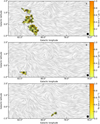 |
Fig. E.1 Same as Fig. 15, but for the other clouds. |
| In the text | |
Current usage metrics show cumulative count of Article Views (full-text article views including HTML views, PDF and ePub downloads, according to the available data) and Abstracts Views on Vision4Press platform.
Data correspond to usage on the plateform after 2015. The current usage metrics is available 48-96 hours after online publication and is updated daily on week days.
Initial download of the metrics may take a while.