| Issue |
A&A
Volume 675, July 2023
|
|
|---|---|---|
| Article Number | A44 | |
| Number of page(s) | 43 | |
| Section | Extragalactic astronomy | |
| DOI | https://doi.org/10.1051/0004-6361/202345912 | |
| Published online | 30 June 2023 | |
Extragalactic fast X-ray transient candidates discovered by Chandra (2014–2022)⋆
1
Instituto de Astrofísica, Pontificia Universidad Católica de Chile, Casilla 306, Santiago 22, Chile
e-mail: This email address is being protected from spambots. You need JavaScript enabled to view it.
2
Millennium Institute of Astrophysics (MAS), Nuncio Monseñor Sótero Sanz 100, Providencia, Santiago, Chile
3
Department of Astrophysics/IMAPP, Radboud University, PO Box 9010 6500 GL Nijmegen, The Netherlands
4
Observatorio Astronómico de Quito, Escuela Politécnica Nacional, 170136 Quito, Ecuador
5
Space Science Institute, 4750 Walnut Street, Suite 205, Boulder, Colorado, 80301
USA
6
SRON Netherlands Institute for Space Research, Niels Bohrweg 4, 2333 CA Leiden, The Netherlands
7
Department of Astronomy & Astrophysics, 525 Davey Laboratory, The Pennsylvania State University, University Park, PA, 16802
USA
8
Institute for Gravitation and the Cosmos, The Pennsylvania State University, University Park, PA, 16802
USA
9
Department of Physics, 104 Davey Laboratory, The Pennsylvania State University, University Park, PA, 16802
USA
10
Kapteyn Astronomical Institute, University of Groningen, PO Box 800 9700 AV Groningen, The Netherlands
11
SRON Netherlands Institute for Space Research, Postbus 800, 9700 AV Groningen, The Netherlands
12
Department of Physics, University of Warwick, Coventry, CV4 7AL
UK
13
CAS Key Laboratory for Research in Galaxies and Cosmology, Department of Astronomy, University of Science and Technology of China, Hefei, 230026
PR China
14
School of Astronomy and Space Science, University of Science and Technology of China, Hefei, 230026
PR China
15
INAF – Brera Astronomical Observatory, Via Bianchi 46, 23807 Merate, LC, Italy
16
Leiden Observatory, Leiden University, PO Box 9513 2300 RA Leiden, The Netherlands
17
School of Astronomy and Space Science, Nanjing University, Nanjing, PR China
18
Key Laboratory of Modern Astronomy and Astrophysics (Nanjing University), Ministry of Education, Nanjing, 210093
PR China
Received:
13
January
2023
Accepted:
26
April
2023
Abstract
Context. Extragalactic fast X-ray transients (FXTs) are short flashes of X-ray photons of unknown origin that last a few minutes to hours.
Aims. We extend the previous search for extragalactic FXTs (based on sources in the Chandra Source Catalog 2.0, CSC2) to further Chandra archival data between 2014 and 2022.
Methods. We extracted X-ray data using a method similar to that employed by CSC2 and applied identical search criteria as in previous work.
Results. We report the detection of eight FXT candidates, with peak 0.3–10 keV fluxes between 1 × 10⁻¹³ to 1 × 10⁻¹¹ erg cm−2 s−1 and T90 values from 0.3 to 12.1 ks. This sample of FXTs likely has redshifts between 0.7 and 1.8. Three FXT candidates exhibit light curves with a plateau (≈1−3 ks duration) followed by a power-law decay and X-ray spectral softening, similar to what was observed for a few before-reported FXTs. In light of the new, expanded source lists (eight FXTs with known redshifts from a previous paper and this work), we have updated the event sky rates derived previously, finding 36.9−8.3+9.7 deg−2 yr−1 for the extragalactic samples for a limiting flux of ≳1 × 10⁻¹³ erg cm−2 s−1, calculated the first FXT X-ray luminosity function, and compared the volumetric density rate between FXTs and other transient classes.
Conclusions. Our latest Chandra-detected extragalactic FXT candidates boost the total Chandra sample by ∼50%, and appear to have a similar diversity of possible progenitors.
Key words: X-rays: bursts
Table 3 is also available at the CDS via anonymous ftp to cdsarc.cds.unistra.fr (130.79.128.5) or via https://cdsarc.cds.unistra.fr/viz-bin/cat/J/A+A/675/A44
© The Authors 2023
 Open Access article, published by EDP Sciences, under the terms of the Creative Commons Attribution License (https://creativecommons.org/licenses/by/4.0), which permits unrestricted use, distribution, and reproduction in any medium, provided the original work is properly cited.
This article is published in open access under the Subscribe to Open model. This email address is being protected from spambots. You need JavaScript enabled to view it. to support open access publication.
1. Introduction
The last decades have seen remarkable progress in understanding the time-resolved sky. Wide-field optical and near-infrared (NIR) surveys identified thousands of supernovae (SNe) and related sources. In the γ-ray regime, the progenitors of both long- and short-duration γ-ray bursts (LGRBs and SGRBs, respectively) have been identified, while in the radio bands decisive inroads have been made into the nature of the fast radio bursts (FRBs). Perhaps surprisingly, our understanding of sources with a similar behavior observed in soft X-rays with the Chandra X-ray Observatory (Chandra), X-ray Multi-mirror Mission-Newton (XMM-Newton), and Neil Gehrels Swift Observatory (Swift-XRT) remains relatively poor. Phenomenologically, we define extra-galactic fast X-ray transients (FXTs) as non-Galactic sources that manifest as nonrepeating flashes of X-ray photons in the soft X-ray regime ∼0.3–10 keV, with durations from minutes to hours (e.g., Alp & Larsson 2020; Quirola-Vásquez et al. 2022). Unfortunately, they still lack a concise or singular physical explanation (e.g., Soderberg et al. 2008; Jonker et al. 2013; Glennie et al. 2015; Irwin et al. 2016; Bauer et al. 2017; Lin et al. 2018, 2019, 2020, 2021, 2022; Xue et al. 2019; Yang et al. 2019; Alp & Larsson 2020; Novara et al. 2020; Ide et al. 2020; Pastor-Marazuela et al. 2020; Quirola-Vásquez et al. 2022).
Critically, while on the order 30 FXTs have been identified to date, both serendipitously and through careful searches, only in one case, XRT 080109/SN 2008D (Soderberg et al. 2008; Mazzali et al. 2008; Modjaz et al. 2009), has there been a detection of a multiwavelength counterpart after the outburst. This is because, in the vast majority of cases, the transients themselves have only been identified long after the outburst via archival data mining (e.g., Alp & Larsson 2020; De Luca et al. 2021; Quirola-Vásquez et al. 2022), so that timely follow-up observations were not possible. Notably, the most stringent limits come from deep optical Very Large Telescope (VLT) imaging serendipitously acquired 80 min after the onset of XRT 141001 (mR > 25.7 AB mag; Bauer et al. 2017). Moreover, only a few of FXTs have had clear host-galaxy associations and even fewer have firm distance constraints (e.g., Soderberg et al. 2008; Irwin et al. 2016; Bauer et al. 2017; Xue et al. 2019; Novara et al. 2020; Lin et al. 2022; Eappachen et al. 2022, 2023; Quirola-Vásquez et al. 2022). Hence, it is not trivial to discern their energetics and distance scale and, by extension, their physical origin.
A variety of different physical mechanisms have been proposed for the origin of FXTs, such as: (i) stochastic outbursts associated with X-ray binaries (XRBs) in nearby galaxies – including subclasses such as ultra-luminous X-ray (ULXs) sources, soft gamma repeaters (SGRs), and anomalous X-ray pulsars (AXPs) – providing possible explanations of FXTs with LX, peak ≲ 1042 erg s−1 (see Colbert & Mushotzky 1999; Kaaret et al. 2006; Woods & Thompson 2006; Miniutti et al. 2019; and references therein); (ii) X-ray emission generated from the shock breakout (SBO; LX, peak ∼ 1042–1045 erg s−1) of a core-collapse supernova (CC-SN) once it crosses the surface of the exploding star (e.g., Soderberg et al. 2008; Nakar & Sari 2010; Waxman 2017; Novara et al. 2020; Alp & Larsson 2020); (iii) off-axis GRBs could explain FXTs (LX, peak ≲ 1045 erg s−1) where the X-ray emission is produced by a wider, mildly relativistic cocoon jet (Lorentz factor of ≲100; Zhang et al. 2004), once it breaks through the surface of a massive progenitor star (Ramirez-Ruiz et al. 2002; Zhang et al. 2004; Nakar 2015; Zhang 2018; D’Elia et al. 2018); (iv) tidal disruption events (TDEs;  and
and  –1050 erg s−1 considering jetted and nonjetted emission, respectively) involving a white dwarf (WD) and an intermediate-mass black hole (IMBH), whereby X-rays are produced by the tidal disruption and subsequent accretion of part of the WD in the gravitational field of the IMBH (e.g., Jonker et al. 2013; Glennie et al. 2015); and (v) mergers of binary neutron stars (BNS; LX, peak ∼ 1044–1051 erg s−1 considering jetted and line-of-sight obscured emission; e.g., Dai et al. 2018; Jonker et al. 2013; Fong et al. 2015; Sun et al. 2017; Bauer et al. 2017; Xue et al. 2019), whereby the X-rays are created by the accretion of fallback material onto the remnant black hole (BH), a wider and mildly relativistic cocoon, or the spin-down magnetar emission (Metzger & Piro 2014; Sun et al. 2017, 2019; Metzger et al. 2018).
In previous work, Quirola-Vásquez et al. (2022, hereafter Paper I) conducted a systematic search for FXTs in the Chandra Source Catalog (Data Release 2.0; 169.6 Ms over 592.4 deg2 using only observations with |b|> 10° and until 2014; Evans et al. 2010, 2019, 2020a), using an X-ray flare search algorithm and incorporating various multiwavelength constraints to rule out Galactic contamination. Paper I reported the detection of 14 FXT candidates (recovering five sources previously identified and classified as FXTs by Jonker et al. 2013; Glennie et al. 2015; Bauer et al. 2017; Lin et al. 2019) with peak fluxes (Fpeak) from 1 × 10⁻¹³ to 2 × 10⁻¹⁰ erg cm−2 s−1 (at energies of 0.5–7 keV) and T90 (measured as the time over which the source emits the central 90%, i.e., from 5% to 95% of its total measured counts) values from 4 to 48 ks. Intriguingly, the sample was subclassified into two groups: six “nearby” FXTs that occurred within d ≲ 100 Mpc and eight “distant” FXTs, likely redshifts ≳0.1. Moreover, after applying completeness corrections, the event rates for the nearby and distant samples became 53.7 and 28.2
 deg−2 yr−1, respectively. However, Paper I does not analyze Chandra observations beyond 2014, implying that several intriguing FXTs likely remain undiscovered.
In this paper, we extend the selection of Paper I to public Chandra observations between 2014 and 2022 using a nearly identical methodology. As in Paper I, this work focuses only on the nonrepeating FXTs, to help reduce sample contamination. We further caution that the sparse nature of repeat X-ray observations means that we cannot rule out that some current FXTs could be repeating FXTs. The study of repeating FXTs is beyond the scope of this paper.
The paper is organized as follows. We explain the methodology and selection criteria in Sect. 2. We present the results of a search and cross-match with other catalogs in Sect. 2.8, a spectral and timing analysis of our final candidates in Sect. 3, and the properties of the identified potential host galaxies in Sect. 4. We explain how we derived local and volumetric rates for the FXTs in Sect. 5. In Sects. 6 and 7, we discuss possible interpretations of some FXTs, and the expected number of FXTs in current and future missions, respectively. Finally, we present comments and conclusions in Sect. 8. Throughout the paper, a concordance cosmology with parameters H0 = 70 km s−1 Mpc−1, ΩM = 0.30, and ΩΛ = 0.70 is adopted. Magnitudes are quoted in the AB system. Unless otherwise stated, all errors are at a 1σ confidence level.
2. Methodology and sample selection
2.1. Identification of X-ray sources
Paper I used as an input catalog of the X-ray sources detected by the CSC2. This is not available for Chandra observations beyond the end of 2014, so a crucial first step is to generate a comparable source detection catalog for the Chandra observations used in this work (see Sect. 2.3), upon which we apply our FXT candidate selection algorithm (Sect. 2.2).
To generate robust X-ray source catalogs, we use the CIAO source detection tool wavdetect (Freeman et al. 2002). It detects possible source pixels using a series of “Mexican Hat” wavelet functions with different pixel bin sizes to account for the varying PSF size across the detector. The wavdetect tool identifies all point sources above a threshold significance of 10−6 (which corresponds to one spurious source in a 1000 × 1000 pixel map) and a list of radii in image pixels from 1 to 32 (to avoid missing detections at large off-axis angles). To avoid erroneous detections, we create exposure and PSF maps, which enable refinement of the source properties. The exposure maps are created by running the fluximage script with the 0.5–7 keV band (Fruscione et al. 2006), while the PSF map, which provides information on the size of the PSF at each pixel in the image, is made using the mkpsfmap task; the PSF size corresponds to the 1σ integrated volume of a 2D Gaussian (Fruscione et al. 2006). The output of the CIAO tool wavdetect is a catalog with essential information about the X-ray sources such as the positions (RA and Dec), positional uncertainty, and significance.
2.2. Transient-candidate selection algorithm
We adopt the same algorithm as presented in Paper I, which augments somewhat the initial version presented in Yang et al. (2019, see their Sect. 2.1 for more details). This method depends on the total (Ntot) and background (Nbkg) counts of the source, working on an unbinned Chandra light curve, which is advantageous because it does not depend on the light curve shapes. The algorithm splits the light curves into different segments in two passes: (i) in two halves and (ii) in three regions, covering the entire Chandra observation. FXT candidates are selected when: (i) Ntot > 5-σ Poisson upper limit of Nbkg to exclude low signal-to-noise ratio (S/N) sources; (ii) the counts in the different segments (Ni) are statistically different at a > 4σ significance level (to select robust detections of short-duration variable sources); and (iii) Ni > 5 × Nj or Nj > 5 × Ni (to select large-amplitude number of counts-variations).
Finally, to mitigate the effect of background (especially for sources with long exposure times and large instrumental off-axis angles), we additionally chop each light curve into 20 ks segments (or time windows Twindow = 20 ks), and reapply the conditions explained above. This reduces the integrated number of background counts per PSF element and thus enables identification of fainter sources at larger instrumental off-axis angles. To maintain an efficient selection of transients across the gaps between these arbitrary windows, we sequence through the entire light curve in three iterations: a forward division in 20 ks intervals, a backward division in 20 ks intervals, and finally, a forward division with a 10 ks shift in 20 ks intervals to cover gaps.
Based on simulations of the CDF-S XT1 and XT2 fiducial light curves (Bauer et al. 2017; Xue et al. 2019), Paper I derived an efficiency of the method of ≳90% for sources with log(Fpeak) > − 12.6 located at off-axis angles  , with a relatively sharp decline in efficiency for FXTs with lower fluxes, for example, ≈50% and ≈5% efficiencies for log(Fpeak) = − 12.8 and log(Fpeak) = − 13.0, respectively, at
  . This instrumental off-axis angle limit is enforced because Chandra’s detection sensitivity (as measured by, e.g., effective area and PSF size) drops significantly beyond this limit (Vito et al. 2016; Yang et al. 2016). Importantly, this algorithm successfully recovered all previously reported sources (XRT 000519, XRT 030511, XRT 110103, XRT 110919, and XRT 141001; Jonker et al. 2013; Glennie et al. 2015; Bauer et al. 2017; Lin et al. 2019; Quirola-Vásquez et al. 2022), and thus is flexible enough to recognize FXTs with different light-curve shapes. We stress that this is a key advantage compared to matched filter techniques that assume an underlying light curve model profile.
2.3. Data selection
To extend the previous search for extragalactic FXTs in Paper I beyond the Chandra Source Catalog 2.0 (CSC2) limit of 2014, we conducted a search through all Chandra ACIS imaging observations (science and calibration observations) made publicly available between 2015 January 1 and 2022 April 1. This includes 3899 individual Chandra-ACIS observations, outside the Galactic plane at |b|> 10 deg, or ≈88.8 Ms, 264.4 deg2 conforming to the following criteria. For uniformity, we consider only ACIS observations in the energy range 0.5–7.0 keV, noting that HRC-I observations comprise only a few percent of the overall observations and have a poorer and softer response and limited energy resolution compared with the ACIS detector. The Chandra observations target a wide variety of astronomical objects, from galaxy clusters to stellar objects. Based on the nature of the extragalactic FXTs identified systematically in Paper I and the potential sources of contamination, we limit our initial light-curve search to sources with Galactic latitudes |b|> 10 deg to reduce the expectedly high contamination rate from flaring stars. An additional benefit of considering objects outside the Galactic plane is that it helps to minimize the effects of Galactic extinction in characterizing the spectral properties of our candidates.
To facilitate our search, we use the full-field per-observation event files available from the Chandra Data Archive products1. Figure 1 shows the cumulative and histogram distributions of exposure time of the Chandra observations used in this work.
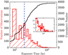 |
Fig. 1. Histogram (red; left Y-axis) and cumulative (black; right Y-axis) distributions of the exposure time of the 3899 Chandra observations used in this work. The inset provides a zoom-in to show the high-exposure time tail of the distribution. The dashed vertical blue line indicates the median exposure time (=19.7 ks) of the total sample. |
2.4. Generation of light curves
The event file contains the relevant stored photon event data, such as photon arrival time, energy, position on the detector, sky coordinates, observing conditions, and the good time interval (GTI) tables listing the start and stop times. To generate light curves, we take X-ray photons in the 0.5–7.0 keV range from each event file using an aperture of 1.5 × R90, where R90 is the radius encircling 90% of the X-ray counts. Based on simulations developed by Yang et al. (2019), the aperture of 1.5 × R90 encircles ≳98% of X-ray counts and depends on the instrumental off-axis angle (and depends on the photon energy; for more details, see Vito et al. 2016; Hickox & Markevitch 2006). We compute Nbkg taking into account an annulus with inner and outer aperture radius of 1.5 × R90 and 1.5 × R90 + 20 pixels, respectively. In the particular case where the background region overlaps with a nearby X-ray source, we mask the nearby source (using a radius of 1.5 × R90), and do not include the masked area to estimate Nbkg. Also, we weigh Nbkg by the source-to-background area ratio to correct the light curve of the sources.
2.5. Astrometry of X-ray sources
To improve upon the nominal absolute astrometric accuracy of Chandra ( (
( ) at 90% (99%) uncertainty)2, we cross-match the detected X-ray sources to optical sources from either the Gaia Early Data Release 3 (Gaia-EDR3; Brown 2021) or Sloan Digital Sky Survey Data Release 16 (SDSS–DR16; Ahumada et al. 2020) catalogs, using the wcs_match script in CIAO. wcs_match compares two sets of source lists from the same sky region and provides translation, rotation and plate-scale corrections to improve the X-ray astrometric reference frame. We adopt a
  matching radius (i.e, ≤8 image pixels), eliminating any source pairs beyond this limit. We typically achieve an accuracy of
  (90% quantile range). This improves our ability to discard contaminants (stellar flares, essentially) and eventually measure projected offsets between X-ray sources and host galaxies (in the case of the final sample of FXT candidates). We combine in quadrature all astrometric errors into the X-ray source positional uncertainty.
2.6. Initial candidate results
As a summary, we apply the FXT detection algorithm to the 0.5–7.0 keV light curves of X-ray sources outside of the Galactic plane (|b|> 10 deg), resulting in 151 FXT candidates. This parent sample has total net counts and instrumental off-axis angles spanning ≈15−33 000 (mean value of 590) and ≈0.12−14.0 (mean value of 5.2) arcmin, respectively. As expected, our selection method identifies FXTs with a wide range of light curve shapes.
2.7. Initial purity criteria
As highlighted in both Yang et al. (2019) and Paper I, our search method does not ensure the unique identification of real extragalactic FXTs. Therefore, it is mandatory to adopt additional criteria considering archival X-ray data and multiwavelength counterparts to differentiate real extragalactic FXTs from Galactic variables and transients among the sample of 151 FXT candidates. We describe and report these additional criteria in Sects. 2.7.1–2.7.5 and summarize the number and percentage, relative to the total, of sources that pass criteria (Col. 5), as well as ignoring all previous steps (Col. 4) in Table 1. Finally, we discuss the completeness of our search and selection criteria in Sect. 2.7.6.
2.7.1. Criterion 1: archival X-ray data
To confirm the transient nature of the FXT candidates, a nondetection in prior and/or subsequent X-ray observations is important. In this way, we consider different observations from Chandra, based on other observations in the CSC2 and individual observations (Evans et al. 2010); XMM-Newton, based on individual observations of sources in the Serendipitous Source (4XMM-DR11; Webb et al. 2020) and Slew Survey Source Catalogues (XMMSL2; Saxton et al. 2008); and the Living Swift XRT Point Source Catalogue (LSXPS) based on observations between 2005-01-01 and 2023-02-12 (Evans et al. 2023). We impose that the FXT candidate remain undetected (i.e., consistent with zero net counts) at 3σ confidence in all X-ray observations, aside from the Chandra observation in which the FXT candidate is detected. This requirement is useful especially to exclude a large number of Galactic stellar flares, but it also may discard FXTs associated with hosts with AGNs, as well as long-lived or recurring X-ray transients (e.g., from SNe in strongly star-forming galaxies). The success of this criterion is related to the number of times a particular field is visited by X-ray facilities.
To discard candidates with prior and subsequent X-ray observations with Chandra, we used the CSC2 or in the cases of candidates with more recent archival observations we downloaded and extracted photometry for these sources, adopting consistent source and background regions and aperture corrections compared to those used in Sect. 2.4. In total, 127 FXT candidates were observed in multiple Chandra observation IDs, while 24 candidates have no additional Chandra observations.
To identify additional XMM-Newton and Swift-XRT detections, we adopt a search cone radius equivalent to the 3σ combined positional errors of the Chandra detection and tentative XMM-Newton or Swift-XRT matches from the 4XMM-DR11, XMMSL2 and LSXPS catalogs, respectively. We additionally search the X-ray upper limit servers: Flux Limits from Images from XMM-Newton using DR7 data (FLIX)3, LSXPS4, and the HIgh-energy LIght curve GeneraTor (HILIGT) upper limit servers5. It is important to mention that HILIGT provides upper limits for several X-ray observatory archives (including XMM-Newton pointed observations and slew surveys; Röntgen Satellite (ROSAT) pointed observations and all-sky survey; Einstein pointed observations), while LSXPS generates Swift-XRT upper limits6.
We found that the reported detections are not always reliable (e.g., inconsistencies between catalogs using the same observations or failure to confirm upon visual inspection), and hence we require detections to be ≥5σ. We found that: 72 candidates are observed in XMM-Newton 4XMM-DR11, with 12 candidates detected; 65 candidates are observed in Swift-XRT LSXPS, with four candidates detected; one candidate is observed in ROSAT pointed observations, with a clear detection; finally, all candidates are observed in the ROSAT All-Sky Survey, with five candidates detected. Also, zero candidates are observed in XMM-Newton XMMSL2 and the Einstein pointed observations. The upper limits from Chandra and XMM-Newton pointed observations are similar to or lower than our FXT candidate peak fluxes. So, we can conclude that similar transient episodes would have been detectable in such observations if present.
In total, 134 candidates have multiple hard X-ray observations by Chandra, XMM-Newton, and/or Swift-XRT, of which 127 candidates have been visited more than once by Chandra. This implies reobserved fractions of at least ≈84% among the candidate sample (a large fraction of this 84% of sources lie in fields intentionally observed multiple times; for instance, in the vicinity of the Orion Nebula or M101). The high X-ray redetection fraction indicates that this is a very effective criterion if additional Chandra, XMM-Newton or Swift observations are available.
In summary, 98 candidates pass this criterion (see Table 1), albeit largely because they lack multiple sensitive X-ray observations. We note that 20 candidates are discarded by this criterion but not by the others (see Table 1). The left panel of Fig. 2 shows the net-count distribution for all the sources that pass this criterion. To conclude, this criterion appears to be an extremely effective means to identify persistent or repeat transients, when data are available.
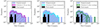 |
Fig. 2. Comparison of 0.5–7.0 keV net-count distributions for the initial (filled blue histograms) and final (filled black histograms) FXT samples, as well as subsets covered by various purity criteria (color non-filled histograms) for the sample. Net counts are provided by the same regions defined in Sect. 2.4. |
2.7.2. Criterion 2: optical detections in Gaia
In previous works (e.g., Paper I and Yang et al. 2019), an important fraction of FXT candidates had a Galactic origin, especially related to relatively bright stars. To identify these, we cross-match with the Gaia Early Data Release 3 (Gaia EDR3; employing the VizieR package; Brown 2021) catalog, which contains photometric and astrometric constraints for sources in the magnitude range G = 3 − 21 mag including accurate positions, parallaxes, and proper motions throughout the Local Group (Lindegren et al. 2018; Gaia Collaboration 2018). We adopt the 3σ positional uncertainty (obtained by the CIAO wavdetect task) associated with each candidate as our cone search radius. In general, this radius is sufficiently small to find a unique counterpart given the high spatial resolution and astrometric precision of Chandra (Rots & Budavári 2011); 9 candidates show multiple Gaia sources in their cone search area, for which we adopt the nearest Gaia source.
From our initial sample of 151 FXT candidates, 107 sources have cross-matches in Gaia EDR3. Nevertheless, we only discard FXT candidates matched to “stellar” Gaia EDR3 optical detections, where stellar is taken to mean those with nonzero proper motion and/or parallax detected at > 3σ significance; this amounts to 83 candidates from the initial sample. These likely stellar sources cover a wide range in magnitude G = 9.2 − 20.1 mag ( mag) and proper motion μ = 0.7 − 154.5 mas yr−1 (
 mas yr−1).
The middle panel of Fig. 2 shows the net-count distribution of the 68 sources that pass this criterion. Among the total sample, ≈55% are associated with stellar flares of bright stars. Moreover, this criterion discards 42 FXT candidates that the additional criteria do not (see Table 1). However, because of the magnitude limit and optical window of Gaia, this criterion may not identify all persistent or recurring transient Galactic objects, which we return to in the next subsection. As a running total, only 42 candidates successfully pass both this and the previous criterion (see Table 1).
2.7.3. Criterion 3: NED, SIMBAD, and VizieR search
To identify known Galactic and Local Group contaminating objects not detected by Gaia, we search for counterparts (or host galaxies) in large databases using the astroquery package: the NASA IPAC Extragalactic Database (NED; Helou et al. 1991), the Set of Identifications, Measurements, and Bibliography for Astronomical Data (SIMBAD; Wenger et al. 2000), and VizieR (which provides the most complete library of published astronomical catalogs; Ochsenbein et al. 2000).
We perform a cone search per FXT candidate, using a circular region with a radius of 3σ based on the X-ray positional uncertainty from the CIAO wavdetect task to find associated sources. These three databases contain many catalogs across the electromagnetic (EM) spectrum, which permit us to rule out candidates in our sample associated with previously classified stars, young stellar objects (YSOs) embedded inside nebulae (where the absorption and obscuration do not permit Gaia detections), globular clusters, or high-mass X-ray binaries (HMXBs) in either our Galaxy or the Local Group. This criterion is important in our analysis because ≈80% (i.e., 121 FXT candidates) of the initial sample show associated sources with the SIMBAD and NED databases. We uniquely identify 33 objects, either as YSOs embedded in nebulae or stars identified by other catalogs, for instance, the VISTA Hemisphere Survey (VHS), the United Kingdom InfraRed Telescope (UKIRT) Infrared Deep Sky Survey, the Sloan Digital Sky Survey (SDSS), or the all-sky Wide-field Infrared Survey Explorer (WISE) CatWISE source catalog at 3.4 and 4.6 μm (McMahon et al. 2013; Dye et al. 2018; Marocco et al. 2021). It is important to mention that 33 FXT candidates are discarded solely by this criterion (see Table 1).
The right panel of Fig. 2 shows the net-count distribution for the 76 FXT candidates that pass this criterion. Applying all criteria thus far, the sample is reduced to nine candidates.
2.7.4. Archival image search
To rule out still fainter stellar counterparts, we carried out a search of ultraviolet (UV), optical, NIR, and mid-infrared (MIR) image archives. We perform a cone search within a radius equivalent to the 3σChandra positional uncertainty of the respective FXTs for the following archives: the Hubble Legacy Archive7; the Pan-STARRS archive (Flewelling et al. 2020)8; the National Science Foundation’s National Optical-Infrared Astronomy Research (NOIR) Astro Data Lab archive9, which includes images from the Dark Energy Survey (DES; Dark Energy Survey Collaboration 2016) and the Legacy Survey (DR8); the Gemini Observatory Archive10; the National Optical Astronomy Observatory (NOAO) science archive11; the ESO archive science portal12; the VISTA Science Archive13; the Spitzer Enhanced Imaging Products archive (Teplitz et al. 2010)14; the UKIRT/Wide Field Camera (WFCAM) Science Archive15; and the WISE archive (Wright et al. 2010).
For images obtained under good seeing (< 1″) and weather conditions, we inspect visually for counterparts or host galaxies in the 3σ uncertainty X-ray location of the FXT. We only apply this additional criteria for the FXT candidates that remain after the previous three criteria (see Sects. 2.7.1–2.7.3). If a source is found, we identify it as a star if it is consistent with the spatial resolution of the imaging, we quantify its significance and assess its extent and radial profile visually. We confirm that none of the nine candidates is associated with stellar sources, leaving the number of candidates unchanged.
2.7.5. Instrumental and variability effects
Finally, we visually check the X-ray data to rule out false-positive candidates that may arise from background flares, bad pixels or columns, or cosmic-ray afterglows rather than intrinsic variability. Again, we only undertake this last criteria for the remaining nine candidates after Sect. 2.7.4.
First, we use the glvary tool to confirm variability using the Gregory–Loredo (G–L) algorithm. The Gregory-Loredo variability algorithm is a commonly used test to detect time variability in sources (Gregory & Loredo 1992)16. This adds a second criterion for variability, increasing the probability that the light curves of our candidate FXTs show strong variability during the observation. Applying the G–L task to our sample of nine FXT candidates, we found that one of them (identified in the Chandra ObsId 16302 at  , δ = −32° 35′15.95″) has a low probability to be a variable source (≈0.1) with a variability index of 217. These results guarantee that this source is inconsistent with flux variability throughout the observation. The remaining eight sources show a clear variability throughout the Chandra observation according to their variable probability (≳0.99) and variability index (≳8) (see Table 2 for more details).
Variability properties of the extragalactic FXT candidates detected and/or discussed in this work obtained by the G–L method, ordered by subsample and date.
Finally, to reject possible strong background flaring episodes in the 0.5−7 keV band, we employ the dmextract and deflare tools to examine the evolution of the background count rate during the observations. None of the FXT candidates is affected by background flares. Furthermore, we confirm visually that the counts from all sources are detected in dozens to hundreds of individual pixels (discarding association with bad columns or hot pixels) tracing out portions of Chandra’s Lissajous dither pattern (appearing as a sinusoidal-like evolution of x and y detector coordinates as a function of time; see Fig. A.2) over their duration, reinforcing that they are astrophysical sources. Therefore, we have a final sample of eight FXTs.
2.7.6. Completeness
It is important to keep in mind that real FXTs may have been ruled out erroneously by the criteria above. To roughly estimate this, we compute the probability that a FXT candidate overlaps with another X-ray source and/or star by chance. Assuming Poisson statistics (i.e., P(k, λ)), the probability of one source (k = 1) being found by chance inside the 3σ localization uncertainty region of another is given by
 (1)
(1)
where λ is the source density of X-ray sources and/or stars on the sky multiplied by the 3σChandra localization uncertainty area. As a reference, the mean density of X-ray sources detected by Chandra, XMM-Newton and Swift-XRT is 0.36, 1.68, and 0.07 arcmin−2, respectively, while the mean density of optical sources detected by Gaia is 2.0 arcmin−2. We use the X-ray detections from the CSC2, 4XMM-DR11 and 2SXPS catalogs (Evans et al. 2010, 2020b; Webb et al. 2020), and the Gaia EDR3 catalog for stars (Brown 2021) to determine the X-ray or optical source densities, respectively. The probability is 0.0024 and 0.0029 for X-ray and optical sources, respectively. Taking into account just the X-ray sources discarded solely by Criteria 1 or 2, 20 and 42 X-ray sources (see Table 1), respectively, we expect ≪1 of these to be ruled out wrongly. If we consider only the 109 X-ray sources which were discarded by both Criteria 1 and 2, the combined probability is 1 × 10⁻⁵, and thus the expected number of erroneously dismissed sources is also ≪1.
Considering the densities of X-ray sources in individual Chandra fields, they span a minimum-maximum density range between 0.0042−2.302 arcmin−2, yielding a probability range of 1.4 × 10⁻⁶ to 0.0505. Thus, under these extreme density conditions, the number of X-ray sources discarded wrongly by Criteria 1 is ≈0.1. This value is relatively low, and thus reinforces the idea that an erroneous rejection is unlikely even in extreme conditions. As an extreme example, we can consider the X-ray positions of CDF-S XT2 and source XID4 Ms256 (≈30 photons detected during the 4 Ms exposure, classified as a normal galaxy; Xue et al. 2011; Luo et al. 2017), which differ by only  . Upon further investigation of the flux and position of the X-ray variability, it was realized that XID4 Ms256 and CDF-S XT2 are distinct sources (Xue et al. 2019). The X-ray source density (at
  off-axis angle) in the Chandra Deep Field South at 7 Ms is ≈5.6 arcmin−2 (Luo et al. 2017), leading to a chance alignment probability (using Eq. (1)) of 0.019 between CDF-S XT2 and ID4 Ms256. Although this value is low, it is nonzero, and thus care should be given to the spatial and/or temporal alignment of X-ray sources, so as to not discard candidates erroneously.
It is not easy to assess the contribution by Criterion 3 to the completeness given the highly disjoint nature of the databases. Similar to Paper I, we assume that Criterion 3 does not disproportionately discard real FXTs. In aggregate, we conclude that our rejection criteria do not apparently impact on the completeness of our FXT candidate sample.
2.7.7. Summary
We identify eight FXT candidates, three of them have been previously discovered and classified as FXTs by Xue et al. (2019), Lin et al. (2021, 2022); see Sect. 2.8 for more details. Table 3 shows important information of the final sample: the coordinates, duration (T90), instrumental off-axis angle, positional uncertainty, hardness ratio (HR; computed following Park et al. 2006), and S/N ratio (computed using the wavdetect tool). Figure 3 shows the background-subtracted 0.5–7.0 keV light curves of our final sample of FXT candidates: short-term, in units of counts (first column) and logarithmic count rates (second column); long-term in units of net-counts for Chandra only (third column) and flux to compare uniformly Chandra, XMM-Newton and Swift-XRT data (fourth column). It is important to mention that the first three criteria considered (X-ray archival data, Gaia detection cross-match, and NED/SIMBAD/VizieR catalogs) contribute significantly and in complementary ways to clean the sample (especially for discarding stellar contamination).
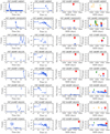 |
Fig. 3. 0.5–7 keV light curves for each FXT candidate: (1st column) full exposure, in units of counts; (2nd column) zoom in, from the detection of first photon to the end of the exposure, in units of count rate (cts s−1), with log-log scaling and 5 counts per bin. The gray dashed lines show the stop-time per observation regarding the beginning of the transient; (3rd column) long-term light curve, with each point representing individual Chandra exposures (cyan circles with 1-σ error bars) to highlight the significance of detections and nondetections, in units of counts; (4th column) long-term light curve, with each point representing individual Chandra (cyan), XMM-Newton (orange) and Swift-XRT (green) exposures in units of flux (erg s−1 cm−2). For the long-term light curves, the observation including the transient is denoted by a large red star (1-σ error bars), while triangles denote observations with (3-σ) upper limits. All fluxes are reported in the 0.5–7 keV band in the observer’s frame. |
Properties of the extragalactic FXT candidates detected and/or discussed in this work, ordered by date.
Finally, we label each FXT candidate by “XRT” followed by the date, where the first two numbers correspond to the year, the second two numbers to the month, and the last two numbers to the day (see Table 3, second column). Nevertheless, similar to Paper I, to identify each source quickly throughout this paper we also denominate them by “FXT”+# (ordered by date; see Table 3, first column) from 15 to 22, because this work is a sequel paper to Paper I where FXTs were labeled until FXT 14. Furthermore, FXT 18 does not have additional Chandra, XMM-Newton or Swift-XRT observations to ensure its transient nature, however, we keep it to be consistent with the selection criteria of this work.
2.8. Fainter electromagnetic detections
We now focus on a detailed multiwavelength search (in Sects. 2.8.1–2.8.4 from radio to γ rays) of each candidate for a contemporaneous counterpart18 and host galaxy using several archival datasets to understand their origin.
2.8.1. Radio emission
We search for any possible radio emission associated to our FXT candidates using the RADIO–Master Radio Catalog, which is a revised master catalog with select parameters from a number of the HEASARC database tables. It holds information on radio sources across a wide range of telescopes and/or surveys (e.g, the Very Long Baseline Array, the Very Large Array (VLA), and the Australia Telescope Compact Array) and frequencies (from 34 MHz to 857 GHz). Because of the poor angular resolution of some associated radio catalogs, we perform an initial cone search for radio sources with a radius of 60 arcsec. Following this initial 60 arcsec cut, we repeat a search using limiting radii consistent with the combined radio + X-ray 3σ positional errors. The current version of the master catalog does not yet contain the recent VLA Sky Survey (VLASS)19 and Rapid ASKAP Continuum Survey (RACS; Hale et al. 2021) catalogs, so we additionally query these using resources from the Canadian Astronomy Data Centre20 interface. Unfortunately, our search returns no matches indicating that none of the final sample of FXT candidates or host sites is unambiguously detected at radio wavelengths.
2.8.2. Optical and mid-Infrared counterpart emission
In order to explore possible optical and MIR contemporaneous counterparts of our final sample, we examine forced differential photometry taken from the Zwicky Transient Facility (ZTF; Bellm et al. 2019; Graham et al. 2019; Masci et al. 2019), the Asteroid Terrestrial-impact Last Alert System (ATLAS; Tonry et al. 2018; Smith et al. 2020), and a visual inspection of images obtained during epochs around the X-ray trigger obtained from the unWISE time-domain (Meisner et al. 2023) and the Legacy Surveys DR10 catalogs (Dey et al. 2019).
ZTF is a wide-field (field of view of 55.0 deg2) time-domain survey, mapping the sky every few nights with custom g, r, and i filters to 5-σ limiting magnitudes of ≈20.8, 20.6, 19.9 AB mag, respectively (Bellm et al. 2019). ATLAS is a four-telescope asteroid impact early warning system, which observes the sky several times every night in custom cyan (c; 420−650 nm) and orange (o; 560−820 nm) filters to 5-σ limiting magnitudes of ≈19.7 AB mag (Tonry et al. 2018; Smith et al. 2020).
Figures 4 and 5 show the differential photometry light curves taken from ZTF (gri) and ATLAS (co), respectively, for the FXT candidates. For visual clarity, the ZTF and ATLAS photometry are binned by 50 days, with the errors added in quadrature. The locations of all eight FXT candidates have been observed by ATLAS (see Fig. 4), although FXT 15 and FXT 16 were not visited by ATLAS around the time of the X-ray detection (highlighted by the vertical blue lines). ZTF, on the other hand, has only observed six FXT candidate locations (see Fig. 5), of which FXT 15, FXT 17 and FXT 18 fields not being observed around the time of the Chandra detection. Notably, the most recent FXTs (FXTs 20, 21 and 22) have forced differential photometry light curves from ZTF and ATLAS, covering a wide epoch both before and after the Chandra X-ray detections. Overall, none of the FXT candidates exhibits significant (> 5σ) detections of optical variability or flares by ZTF and ATLAS around the time of the FXT candidate X-ray trigger, nor are there any robust detections in any previous or subsequent epochs. We derive 3σ upper limits from the closest observation taken by ZTF and ATLAS (for the available filters and FXTs), as listed in Table B.1.
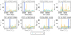 |
Fig. 4. ATLAS differential photometry of the cyan (c) and orange (o)-bands light curves performed at the position of the FXT candidates. < 5σ data points are shown in hollow circles, while > 5σ data points are shown in solid circles. The blue vertical lines show the epochs when the FXT candidates were detected by Chandra, while the dashed gray lines represent the zero flux. |
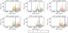 |
Fig. 5. ZTF differential photometry of the g (green points), r (red points) and i-bands (orange points) light curves performed at the position of the FXT candidates. < 5σ data points are shown in hollow circles, while > 5σ data points are shown in solid circles. The blue vertical lines shows the epochs when the FXT candidates were detected by Chandra, while the dashed gray lines represents the zero flux. |
To check if the forced photometry is consistent with zero flux (around the X-ray trigger), we use the statistical test CONTEST (Stoppa et al. 2023), developed explicitly to compare the consistency between the observations and a constant zero flux model. We adopt a methodology identical to that discussed in Eappachen et al. (2023). We applied this test considering two-time windows, [−10; 20] and [−10; 100] days, with respect to the X-ray trigger, because possible optical counterparts have timescales from days (e.g., the afterglow of GRBs) to weeks and months (e.g., CC-SNe emission). We concluded that for all the sources, the model of zero flux density detected by both periods is consistent with the observations.
Furthermore, the DESI Legacy Imaging Surveys (DR10) combine three major public projects plus additional archival data to provide imaging over a large portion of the extragalactic sky visible from the Northern and Southern Hemispheres in at least three optical bands (g, r, and z). The sky coverage (∼30 000 deg2) is approximately bound by −90° < δ < +84° in celestial coordinates and |b|> 15° in Galactic coordinates (Dey et al. 2019). Thus, the Legacy Imaging survey observes most FXT locations (except for FXTs 17 and 21). We explore visually each individual imaging epoch provided by the Legacy survey in g-, r-, i-, and z-bands to identify potential optical contemporaneous counterparts of the FXTs. However, no contemporaneous optical counterparts are identified around the X-ray trigger time after a visual inspection.
The Wide-field Infrared Survey Explorer (WISE; Wright et al. 2010) provides an unprecedented time-domain view of the MIR sky at W1 = 3.4 μm and W2 = 4.6 μm due to the NEOWISE mission extension (Mainzer et al. 2011, 2014). WISE has completed more than 19 full-sky epochs over a > 12.5 year baseline, with each location having been observed for ≳12 single exposures (Meisner et al. 2023). In order to search for a potential counterpart inside the WISE and NEOWISE images, we use the time-domain API tools provided by the unTimely Catalog, which considers data from 2010 to 2020 (Meisner et al. 2023). We visually inspect each single-epoch image of each FXT field (for FXT 22, only up to ∼1.5 years before the X-ray trigger). Unfortunately, none of the FXT candidates shows significant detections of variability or flares around the time of the X-ray trigger.
2.8.3. Ultraviolet, optical, and infrared host galaxy identification
To search for UV, optical, NIR and MIR emission associated with any possible host galaxy in the vicinity of each FXT candidate, we perform a cone search within a radius equivalent to the 3σChandra error position (see Table 3) in the following catalogs: GALEX Data Release 5 (GR5; Bianchi et al. 2011), Pan-STARRS Data Release 2 (Pan-STARRS–DR2; Flewelling 2018), the DES Data Release 2 (DES–DR2; Abbott et al. 2021), the SDSS Data Release 16 (SDSS–DR16; Ahumada et al. 2020), the NOAO Source Catalog Data Release 2 (NSC–DR2; Nidever et al. 2021), the Hubble Source Catalog version 3 (HSCv3; Whitmore et al. 2016), the UKIRT InfraRed Deep Sky Survey Data Release 11+(UKIDSS–DR11+; Warren et al. 2007), the UKIRT Hemisphere Survey Data Release 1 (UHS–DR1; Dye et al. 2018), the Two Micron All Sky Survey (2MASS; Skrutskie et al. 2006), the VHS band-merged multi-waveband catalogs Data Release 5 (DR5; McMahon et al. 2013), the Spitzer Enhanced Imaging Products Source List (Teplitz et al. 2010), and the unWISE (unWISE; Schlafly et al. 2019) and CatWISE (McMahon et al. 2013; Dye et al. 2018; Marocco et al. 2021) catalogs, as well as the ESO Catalogue Facility and the NED (Helou et al. 1991), SIMBAD (Wenger et al. 2000), and VizieR (Ochsenbein et al. 2000) databases. We supplement this by including any extended sources found during our archival image analysis in Sect. 2.7.4. We assume that uncertainties in the UV through MIR centroid positions contribute negligibly to the overall error budget. Figure 6 shows image cutouts of the localization region of the FXTs (one per row), typically from Pan-STARRS, DECam, or HST in the optical (1st–4th columns, using g, r, i and z or the corresponding HST filters), VISTA, UKIRT, 2MASS or HST in the NIR (5th and 6th columns, using J, H, K or the corresponding HST filters), unWISE in the MIR (7th column, in the 3.6 μm filter) band, and the Chandra-ACIS image (8th column, in the 0.5−7.0 keV band).
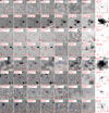 |
Fig. 6. Archival optical, near-infrared, mid-infrared and X-ray images of extragalactic FXT candidates; the telescope/instrument + filter and FXT ID name are shown in the upper-left corner. Each cutout is centered on the X-ray position, while red circles denote 2σChandra errors in the source localization (1st, 2nd, 3rd and 4th columns) optical band (DECam, Pan-STARRS and HST) images (5th and 6th columns) near-infrared J or H and K (2MASS, UKIRT or VISTA) images; (7th column) 3.4 μm (unWISE) images; and (8th column) X-ray Chandra (ACIS) 0.5–7 keV images. The colored arrows and circles show the localization of the possible host of the FXT candidates. HST images were aligned using the astrometry of Gaia. |
FXT 15 has no optical and NIR sources detected within the 3σ X-ray positional uncertainty of this source in the HST, DECam, 2MASS, or unWISE images (see Fig. 6). Upper limits are given in Table 4.
Host and/or counterpart’s photometric data or upper limits of FXT candidates.
FXT 16/CDF-S XT2 (identified previously by Zheng et al. 2017 and analyzed in detail by Xue et al. 2019) was detected by Chandra with a 2σ positional uncertainty of  (see Table 3). This accurate Chandra X-ray position allows us to identify the host galaxy, which lies at an offset of
  (i.e., a projected distance of ≈3.3 kpc) using HST images (see Fig. 6). The galaxy has a spectroscopic redshift of zspec = 0.738. The probability of a random match between FXT 16 and a galaxy as bright as or brighter than mF160W ≈ 24 AB mag within
  is ≈0.01 (Xue et al. 2019).
FXT 17 does not have optical and NIR sources detected within the 3σ X-ray error region of this source in the Pan-STARRS, 2MASS, or unWISE images (see Fig. 6). Upper limits are given in Table 4.
For FXT 18, one faint source with mr ≈ 24.2 AB mag (see Fig. 6, source #1) appears inside the large localization region ( at 3σ) in the DECam g, r, i and z-band images with an off-set angle of
  from the X-ray center position; it has a chance association probability of < 0.095. Two other sources lie slightly outside the X-ray uncertainty region, sources #2 and #3, with chance probabilities of 0.582 and 0.363, respectively (see Fig. 6); such high probabilities suggest an association with either one of them is unlikely.
FXT 19 (reported previously by Lin et al. 2019 and analyzed in detail by Lin et al. 2022) lies close to a faint (mF606W ≈ 24.8, mF814W ≈ 24.9, mF110W ≈ 24.7 and mF160W ≈ 24.3 AB mag, using aperture photometry) and extended optical and NIR source in HST imaging (see Fig. 6, source #1) with an angular offset  . The chance probability for FXT 19 and source #1 to be randomly aligned in F160W is very low, only 0.005 (Lin et al. 2022).
FXT 20 was detected  (or ≈500 kpc in projection) from the center of the galaxy cluster Abell 1795 (located at ≈285.7 Mpc) during a Chandra calibration observation (ObsId 21831). FXT 20 lies close to a faint source mr ≈ 23.5 AB mag (see Fig. 6, source #1) identified in DECam g, r, and z-bands at an offset angle of
  . The probability of a false match is P < 0.005 (adopting the formalism developed by Bloom et al. 2002) for such offsets from similar or brighter objects.
FXT 21 has a faint optical source (mr ≈ 25.1 AB mag) inside the 3σ X-ray error position in Pan-STARRS images (see Fig. 6, source #1), but no source is detected in 2MASS NIR or unWISE MIR images. The offset between the FXT and the optical source position is  , with a false match probability of P < 0.0085 (adopting the formalism developed by Bloom et al. 2002) for such offsets from similar or brighter objects.
Finally, FXT 22 (identified previously by Lin et al. 2021) was detected  (or ≈300 kpc in projection) from the center of the galaxy cluster Abell 1795 (located at ≈285.7 Mpc) during a Chandra calibration observation (ObsId 24604). No sources are detected within the 3σ X-ray error region of this source in the DECam optical, VISTA NIR, or unWISE MIR images (see Fig. 6). However, this source falls close to an extended object, SDSS J134856.75+263946.7, with mr ≈ 21.4 AB mag that lies at a distance of
  from the position of the FXT (≈40 kpc in projection) with a spectroscopic redshift of zspec = 1.5105 (Andreoni et al. 2021; Jonker et al. 2021; Eappachen et al. 2023). The probability of a false match is P < 0.041 (adopting the formalism developed by Bloom et al. 2002) for such offsets from similar or brighter objects.
To summarize, we conclude that four (FXTs 16, 19, 20 and 21) of the eight FXT candidates have high probabilities of being associated with faint (FXT 20) or moderately bright (FXTs 16, 19, and 21) extended sources within the 3σ positional error circle. In the case of FXT 22, it may be associated with the extended source SDSS J134856.75+263946.7 (zspec = 1.5105); nevertheless, a relation with a faint background source cannot be excluded (a faint extended source is in the X-ray uncertainty region; Eappachen et al. 2023). In the case of FXT 18, its large positional uncertainty does not allow us to determine robustly the counterpart optical or NIR source. Finally, two FXT candidates (FXTs 15 and 17) have no associated optical or NIR sources in the available moderate-depth archival imaging, and remain likely extragalactic FXTs. None of the FXT candidates analyzed in this work appear to be associated with a nearby galaxy (≲100 Mpc). In Sect. 3.4, we explore a scenario where these sources are related to Galactic stellar flares from faint stars.
2.8.4. Higher energy counterparts
To explore if hard X-ray and γ-ray observations covered the sky locations of the FXTs, we developed a cone search in the Nuclear Spectroscopic Telescope Array (NuStar; Harrison et al. 2013), Swift-Burst Alert Telescope (Swift-BAT; Sakamoto et al. 2008), INTErnational Gamma-Ray Astrophysics Laboratory (INTEGRAL; Rau et al. 2005), High Energy Transient Explorer 2 (HETE-2; Hurley et al. 2011), InterPlanetary Network (Ajello et al. 2019), and Fermi (von Kienlin et al. 2014; Narayana Bhat et al. 2016) archives. We adopt a  search radius for the INTEGRAL, Swift-BAT, HETE-2 and Interplanetary Network Gamma-Ray Bursts catalogs, while for the Gamma-ray Burst Monitor (GBM) and the Large Area Telescope (LAT) Fermi Burst catalogs we consider a cone search radius of 4 deg (which is roughly the typical positional error at 1σ confidence level for those detectors; Connaughton et al. 2015). Additionally, we implement a time constraint criterion of ±15 days in our search between Γ-ray and FXT triggers.
To further probe whether there may be weak γ-ray emission below the trigger criteria of Fermi-GBM at the location of the FXTs, we investigated the Fermi-GBM daily data, the Fermi position history files21, and the GBM Data Tools (Goldstein et al. 2022)22. We confirmed that FXTs 15, 16, 17, 20, and 21 were in the FoV of Fermi-GBM instruments during the X-ray trigger time ±50 s, while FXTs 18, 19, and 22 were behind the Earth around the X-ray burst trigger time; thus, their fields were not visible. Table A.1 summarizes the visibility of the sources and the Fermi-GBM instruments covering the fields around the X-ray trigger time (at a distance of ≲60°). In summary, we find no hard X-ray or γ-ray counterparts associated with NuSTAR, INTEGRAL, Swift-BAT, HETE-2, Interplanetary Network and the GBM and LAT Fermi Burst catalogs, but cannot rule out weak γ-ray emission for FXTs 18, 19, and 22.
3. Spatial, temporal and X-ray spectral properties
We analyze the spatial distribution of our final sample of FXT candidates in Sect. 3.1. Furthermore, the time evolution and spectral properties could give important information about the physical processes behind the FXT candidates, and thus we explore and describe these in Sects. 3.2 and 3.3, respectively. Finally, we explore a Galactic stellar flare origin of this sample in Sect. 3.4.
3.1. Spatial properties
If the FXT candidates are extragalactic and arise from large distances, then given the isotropy of the universe on large scales, we expect them to be randomly distributed on the sky. Figure 7 shows the locations, in Galactic coordinates, of the final FXT candidates of Paper I and this work, the initial FXT candidates of this work, and the Chandra observations analyzed in Paper I and this work. We investigate the randomness of the FXT candidate distribution on the sky compared to all Chandra observations considered in this work. For this, we use the non-parametric Kolmogorov–Smirnov (K–S) test (Kolmogorov 1933; Massey 1951; Ishak 2017).
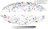 |
Fig. 7. Sky positions, in Galactic coordinate projection, of FXT candidates: the initial 151 FXT candidates of this work are represented by blue triangles (see Sect. 2.6; some symbols overlap on the sky); the final sample of eight extragalactic FXT candidates from this work are denoted by large red stars (FXTs 20 and 22 overlap on this scale); and the final sample of 14 extragalactic FXTs analyzed in Paper I are shown as orange circles (FXTs 14 and 16 overlap on this scale). The background gray scale encodes the location and number of distinct colocated or closely located observations among the combined 3899 and 5303 Chandra observations used in this work and Paper I, respectively. |
We explore the randomness of the spatial distribution of our final sample of eight FXTs. For this, we simulate 10 000 samples of 40 000 random sources distributed over the sky, taking as a prior distribution the Chandra sky positions used in this work (which are functions of the pointings and exposures). Out of these fake sources, we randomly select eight sources, which we compare to the spatial distribution of the eight real FXT candidates using a 2D K–S test (following the methods developed by Peacock 1983; Fasano & Franceschini 1987). We can reject the 𝒩ℋ that these sources are drawn from the same (random) distribution only in ≈0.2% of the draws. Therefore, the positions of the eight FXT candidates are consistent with being randomly distributed over the total Chandra observations on the sky.
Intriguingly, FXTs 14 and 16 lie in the same field of view (i.e., in the Chandra Deep Field South), as do FXTs 20 and 22 (i.e., in the direction of the galaxy cluster Abell 1795). Thus, we explore the probability that two FXTs occur in the same field, which is given by the Poisson statistic (i.e., P(k, α), using Eq. (1)), where k = 2 and α is the ratio between the total Chandra exposure time in a particular field (for the Chandra Deep Field South and the cluster Abell 1795 are 6.8 and 3.1 Ms, respectively23) and the total Chandra exposure time analyzed in Paper I and this work (≈169.6 and 88.8 Ms, respectively) normalized to the total number of FXTs identified (i.e., 22 FXTs). The chance probabilities for FXTs 14, 16 and 20, 22 are 0.115 and 0.029, respectively. We can conclude that the occurrence of two FXTs being found in these particular fields is unusual, but not ruled out at high significance.
3.2. Temporal properties
To characterize and measure the break times and light-curve slopes in the X-ray light curves of the candidate FXTs, we consider a single power-law (PL) model with index τ1, or a broken power-law (BPL) model with indices τ1, τ2 and break time Tbreak (for more detail, see Paper I, Sect. 3.2)24.
Both models describe well the majority of the FXT X-ray light curves in this work. To fit the data, we use the least-square method implemented by the lmfit Python package25. The best-fit model parameters and statistics are given in Table 5, while the light curves (in flux units; light curves have five counts per bin) and best-fit models are shown in Fig. 8. We define the light-curve zeropoint (T0 = 0 s) as the time when the count rate is 3σ higher than the Poisson background level (see Table 5). To confirm the zeropoint, we divide the light curves in bins of Δt = 100 and 10 s, and compute the chance probability that the photons per bin come from the background (Pbkg)26. We found that the bins after T0 have a Pbkg ≲ 0.01, while Pbkg immediately before T0 is higher Pbkg ≳ 0.1 − 0.2. We use the Bayesian Information Criterion (BIC)27 to understand which of the two models describes better the data. We consider the threshold criterion of ΔBIC = BICh–BICl > 2 to discriminate when comparing two different models, where BICh is the higher model BIC, and BICl is the lower model BIC. The larger ΔBIC, the stronger the evidence against the model with a higher BIC is (Liddle 2007).
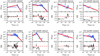 |
Fig. 8. Light curve and hardness evolution. Top panels: observed 0.5–7.0 keV X-ray light curves in cgs units (blue points), starting at T = 20 s. We also plot the best-fit broken power-law or simple power-law model (red solid lines). The light curves contain five counts per bin. Bottom panels: hardness ratio evolution (the soft and hard energy bands are 0.5–2.0 keV and 2.0–7.0 keV, respectively), following the Bayesian method of Park et al. (2006). The red dashed line denotes a hardness ratio equal to zero. Here, T0 = 0 s is defined as the time when the count rate is 3σ higher than the Poisson background level. |
Best-fit parameters obtained using either a broken power-law (BPL) or a power-law (PL) model fit the X-ray light curves.
The parameters of the best-fitting models of the light curves are listed in Table 5, while Fig. 8 shows the best-fit broken power-law or simple power-law models. Five sources (FXTs 15, 16, 19, 20, and 22) require a break time (based on the BIC criterion), while three do not (FXTs 17, 18, and 21). In two of the former (FXT 15 and 20), τ1 is negative, indicating a discernible rise phase; the other three (FXTs 16, 19, and 22) are consistent with an early plateau phase.
3.3. Spectral properties
Using X-ray spectra and response matrices generated following standard procedures for point-like sources using CIAO with the specextract script, we analyze the spectral parameters of the FXT candidates. The source and background regions are the same as those previously generated for the light curves (see Sect. 2.4). To find the best-fit model, because of the low number of counts, we consider the maximum likelihood statistics for a Poisson distribution called Cash-statistics (C-stat.; Cash 1979)28. Because of the Poisson nature of the X-ray spectral data, the C-stat. is not distributed like χ2 and the standard goodness-of-fit is inapplicable (Buchner et al. 2014; Kaastra 2017). Thus, similarly to Paper I, we use the Bayesian X-ray Astronomy package (BXA; Buchner et al. 2014), which joins the Monte Carlo nested sampling algorithm MultiNest (Feroz et al. 2009) with the fitting environment of XSPEC (Arnaud 1996). BXA computes the integrals over the parameter space, called the evidence (𝒵), which is maximized for the best-fit model, and assuming uniform model priors.
We consider one simple continuum model: an absorbed power-law model (phabs*zphabs*po, hereafter the PO model), which is typically thought to be produced by a nonthermal electron distribution. We choose this simple model because we do not know the origin and the processes behind the emission of FXTs. Furthermore, the low number of counts does not warrant more complex models. The spectral absorption components phabs and zphabs represent the Galactic and intrinsic contribution to the total absorption, respectively. During the fitting process, the Galactic absorption (NH, Gal) was fixed according to the values of Kalberla et al. (2005) and Kalberla & Haud (2015), while for the intrinsic neutral hydrogen column density (NH), we carried out fits for both z = 0 (which provides a lower bound on NH since firm redshifts are generally not known, and is useful for comparison with host-less FXTs) and the redshift values from Table 6 or fiducial values of z = 1 for host-less sources.
Parameters obtained from the literature and by our SED fitting to archival photometric data using the BAGPIPES package (Carnall et al. 2018).
The best-fitting absorbed power-law models (and their residuals) and their parameters are provided in Fig. 9 and Table 7, respectively; additionally, Fig. 10 shows the histograms of the best-fit intrinsic neutral hydrogen column densities (NH; top panel) and photon index (Γ; bottom panel) for extragalactic FXTs candidates of this paper (orange histograms) and from Paper I (blue histograms). The candidates show a range of NH ≈ (1.1 − 18.1)×1021 cm−2 (assuming z = 0), and a mean value of  cm−2, consistent with the range for sources reported by Paper I (see Fig. 10, top panel). We note that in all cases here, the best-fit NH is higher than the NH, Gal estimates from Kalberla et al. (2005) and Kalberla & Haud (2015) by a factor of ≈4−90. In every case, intrinsic absorption and the Galactic component are needed, with at least ≈95% confidence, and in some cases even ≈99% confidence level. Therefore, two absorption components are needed in the fitting process in general.
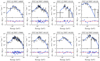 |
Fig. 9. X-ray spectra per FXT candidates. Top panels: X-ray spectra (black crosses), in units of counts s−1 keV−1. We also plot the best-fit absorbed power-law (blue lines) spectral model; see Table 7 for the corresponding best-fitting parameters. Bottom panels: residuals (defined as data-model normalized by the uncertainty) of each spectral model. |
Results of the 0.5–7 keV X-ray spectral fits for the final sample of FXT candidates.
Furthermore, excluding the soft candidate FXT 18, the best-fit power-law photon index ranges between Γ ≈ 2.1 − 3.4 for the candidate FXTs, with a mean value of  . FXT 18 is an exceptionally soft source (Γ ≳ 6.5) compared to both this sample and the FXT candidates presented in Paper I (see Fig. 10, bottom panel). Finally, FXTs 17, 18, and 21, whose light curves are best-fitted by a PL model, have some of the softest photon indices (Γ ≳ 3).
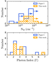 |
Fig. 10. Power-law spectral parameters. Top panel: intrinsic neutral hydrogen column density distribution, evaluated at z = 0 and in units of cm−2, obtained using the power-Law model for extragalactic FXT candidates from this work (orange histogram) and Paper I (blue histogram). The arrows indicate that the z = 0 intrinsic hydrogen column densities are lower bounds. Bottom panel: photon index distribution, obtained using a power-law model, for FXT candidates from this work (orange histogram) and Paper I (blue histogram). Note that the uncertainties on these parameter values for individual sources can be considerable (see Table 7). |
3.3.1. Hardness ratio and photon index evolution
The hardness ratio (HR) can be used to distinguish between X-ray sources, and permit us to explore their spectral evolution, especially in cases with low-count statistics (e.g., Lin et al. 2012; Peretz & Behar 2018). In this work, the HR is defined as:
 (2)
(2)
where H and S are the number of X-ray photons in the 0.5–2.0 keV soft and 2.0–7.0 keV hard energy bands. For each source candidate, we calculate the HR using the Bayesian code BEHR (Park et al. 2006), which we list in Table 3, Col. 11, and plot in Fig. 11 (top panel).
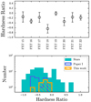 |
Fig. 11. Hardness ratio comparison. Top panel: hardness ratio of each FXT candidate (using the Bayesian BEHR code; Park et al. 2006) at 1σ confidence level. Bottom panel: hardness-ratio distributions of our final samples of FXTs (orange histogram), compared to the X-ray transients classified as “stars” by Criterion 2 using Gaia (filled cyan histogram) and the sources identified previously as distant FXTs (blue histogram) by Paper I. |
We compare the HR of the 90 objects identified as “stars” by Criterion 2 (see Fig. 11, bottom panel, cyan histogram) in Sect. 2.7.2 with the final sample of FXTs in this work (orange histogram) and the sample of FXTs reported by Paper I (blue histogram). Stars typically have very soft X-ray spectra (Güdel & Nazé 2009), confirmed by the fact that ≈90% of the star candidates strongly skew toward soft HRs (≲0.0). Clearly, Fig. 11 shows that FXTs do not stand out in the HR plane; thus, HR is not a useful discriminator on its own between stellar contamination and extragalactic FXTs.
We also analyze how the HR and power-law index of the X-ray spectrum change with time. To this end, we compute the time-dependent HR, with the requirement of 10 counts per time bin from the source region (to improve the statistics), which we show in the lower panels of Fig. 8. For sources that are well-fit by a BPL model, we also split the event files at Tbreak and extract and fit the spectra to compute spectral slopes “before” and “after” Tbreak (Γbefore and Γafter, respectively; see Table 8) using the value for the absorption derived from the fit to the full spectrum (see Table 7). We fit both spectral intervals together assuming fixed, constant NH, Gal and NH (taken from Table 7).
Spectral photon index before and after the break time.
The spectra of FXT 16 clearly softens after the plateau phase (Fig. 8 and Table 8) at > 90% confidence. Similar spectral evolution was also seen from previous FXT candidates XRT 030511 and XRT 110919 (Paper I). FXTs 15 and 20 exhibit similar spectral softening trends, with Tbreak as a pivot time, although with only marginal significance, while the rest show no obvious evidence of such trends (Fig. 8 and Table 8). Finally, it is important to mention that the FXTs whose light curves follow a PL model (FXTs 17, 18, and 21) show hardening trends in their HR evolution (see Fig. 8).
3.4. Galactic origin
From our sample, FXTs 16 and 19 are clearly aligned with extended objects, proving an extragalactic origin. FXTs 18, 20, 21, and 22, based on their low random match probabilities, could be associated with potential hosts, supporting an extragalactic association (see Sect. 2.8 for more details). In the next paragraphs, similar to Paper I (see its Sect. 3.4 for more details), we explore any of the FXT candidates could still be associated with magnetically active M- or brown-dwarf flares, which are known to produce X-ray flares on timescales of minutes to hours, with flux enhancements up to two orders of magnitude (not only at X-ray wavelengths; Schmitt & Liefke 2004; Mitra-Kraev et al. 2005; Berger 2006; Welsh et al. 2007).
Stellar flares typically show soft thermal spectra with temperatures on the order of kT ∼ 0.5 − 1 keV. M-dwarf stars (brown-dwarfs) have optical and NIR absolute magnitudes in the range of Mz ∼ 8 − 13 AB mag (Mz ∼ 13 − 18 AB mag) and MKs ∼ 3 − 10 AB mag (MJ ∼ 15 − 25 AB mag), respectively (Hawley et al. 2002; Avenhaus et al. 2012; Tinney et al. 2014).
The enhanced X-ray emission of M dwarfs shows flares on the order of  –1032 erg s−1 (Pallavicini et al. 1990; Pandey & Singh 2008; Pye et al. 2015), while brown dwarf flares cover a luminosity range of
  –1030 erg s−1 (Berger 2006; Robrade et al. 2010). Empirically, the ratio between the X-ray luminosity (LX) and bolometric luminosity (Lbol) of cool M dwarfs and L dwarfs typically exhibits values no larger than log(LX/Lbol)≲0.0 and ≲ − 3.0, respectively (e.g., García-Alvarez et al. 2008; De Luca et al. 2020). Adopting this limiting ratio, we rule out a stellar flare scenario for FXT candidates. As in Paper I, we compute the ratio log(LX/Lbol) considering stellar synthetic models of dwarf stars (taken from Phillips et al. 2020, 1000 ≲ Teff ≲ 3000 K and 2.5 ≲ log g ≲ 5.5), normalized to the deepest photometric upper limits and/or detections (as listed in Table 4), and compute bolometric fluxes by integrating the normalized models. We describe the constraints for each FXT below:
For FXT 15, the mg > 24.0 and mr > 23.0 AB mag limits imply distances to any putative M- and brown dwarfs responsible for the X-ray flares of ≳0.2−1.7 kpc and ≳0.02−0.2 kpc, respectively. The corresponding X-ray flare luminosities would be  and
and  erg s−1, respectively. These are not enough to discard a Galactic stellar flare nature. Furthermore, the ratio log(FX/Fbol)≳ − 0.9 to −1.4 remains consistent with the extreme spectral type L1 stars (e.g., J0331–27 with log(FX/Fbol)∼0.0; De Luca et al. 2020). Thus, we cannot completely rule out an extreme stellar flare origin for FXT 15.
In the case of FXT 17, the mg > 24.1 and mr > 22.4 AB mag limits imply distances of > 0.2−1.8 kpc and > 0.02−0.2 kpc for M- and brown-dwarfs, respectively, and corresponding X-ray flare luminosities are  and
and  erg s−1, respectively. The X-ray-to-total flux ratio is log(FX/Fbol)≳ − 0.1 to +0.4. Based on these, we cannot discard a Galactic stellar flare association for FXT 17.
For FXT 18, due to the large X-ray positional uncertainty, there are several possible optical counterparts. We consider only source #1 here, as it is closest, lying inside the 2σ X-ray uncertainty position (see Fig. 6). The mg = 24.6 and mi = 24.9 AB mag DECam detections (see Table 4) implies distances of ≈0.3−3.1 kpc and ≈0.03−0.3 kpc for M- and brown-dwarfs, respectively, and corresponding X-ray flare luminosities of  and
and  erg s−1, respectively. The ratio log(FX/Fbol) is ≈2.5 to 3.0. These allow us to rule out robustly any Galactic stellar flare origin.
In the case of FXT 20, we consider source #1 for the stellar flaring analysis (see Fig. 6). The detections mg = 24.3 and mr = 23.5 AB mag equate to distance ranges of ≈0.2−2.5 kpc and ≈0.02−0.3 kpc for M- and brown-dwarfs, respectively, and corresponding X-ray flare luminosities of  and
and  erg s−1, respectively. The ratio log(FX/Fbol) is ≈0.9 to 1.4. These allow us to discard a Galactic stellar flare origin for FXT 20.
Finally, for FXT 21, the mi = 22.7 AB mag Pan-STARRS detection yields distance ranges of ≈0.4−4.1 kpc and ≈0.04−0.4 kpc for M- and brown-dwarfs, respectively, and corresponding X-ray flare luminosities of  and
and  erg s−1, respectively. The ratio log(FX/Fbol) is ≈0.2 to 0.7. Thus, we can rule out FXT 21 as a stellar flare.
In summary, the multiwavelength photometry indicates that three FXTs (FXTs 18, 20, and 21) appear inconsistent with stellar flaring episodes from Galactic M dwarfs and brown dwarfs, while deeper observations are required to completely rule out this option for FXTs 15 and 17.
3.5. One population of FXTs
In Paper I, we found that the FXT candidates could be robustly classified into local and distant populations (see their Sect. 3.5) based on the proximity of some sources to local galaxies (distances ≲100 Mpc). In contrast, we find no plausible and robust association between our final sample and local galaxies in the current work. Two FXT candidates, XRT 191127 and XRT 210423, are detected at projected distances of ≈500 and 300 kpc, respectively, from the center of the galaxy cluster Abell 1795 (≈285.7 Mpc). However, neither is obviously associated with cluster members and physical offsets in this range are not easily explained by any possible physical scenario of FXTs (see Sect. 6).
The lack of local FXTs could be explained by the Chandra exposure time spent observing local galaxies in recent years. Around 26.5% of the Chandra ObsIds (amounting to ≈0.8 years of exposure and a sky area of ≈66.7 deg2) analyzed in this work covers local galaxies (based on a match with the GLADE catalog; Dálya et al. 2018). Adopting the local FXT rate from Paper I,  deg−2 yr−1, we thus expect ≈2.8
 local FXTs in this work, which remains consistent with our nondetection of local FXTs at 3σ confidence for Poisson statistics. On the other hand, the distant FXTs rate from Paper I is
  deg−2 yr−1, implying ≈4.5
 sources, which is consistent with our new eight FXT candidates.
4. Host-galaxy features
The host galaxy or host environment can provide additional information about the nature and origin of this FXT sample. Five FXTs (16, 19, 20, 21, and 22) lie close to extended optical/NIR sources, which are plausible host galaxies (see Fig. 6). The host galaxies of FXTs 19 and 22 were previously identified, but their properties were not reported so far. For FXT 18, just one faint source (source #1) falls inside the X-ray uncertainty position, but it is not clear whether it is extended.
As a first step, in Fig. 12, we explore the nature of the hosts using i − Ks versus g − i (top panel) and i − W1 versus g − i (bottom panel) colors, compared to the colors of X-ray sources previously classified as stars both in Paper I (gray points) and this work (black points; see Sect. 2.7.2), and the expected parameter space for stars (cyan regions) with different ages [log(Age yr−1) = 7.0 − 10.3], metallicities (from [Fe/H] = −3.0 − 0.5), and attenuations (AV = 0.0 − 5.0 mag) from theoretical stellar isochrones (MIST; Dotter 2016; Choi et al. 2016). The vast majority of the X-ray flares with stellar counterparts form a tight sequence (see Fig. 12, cyan region), with the outliers identified as PNe, YSOs, eruptive variable stars, T Tauri stars, or emission-line stars. Overall, the potential hosts of the FXT candidates appear to reside outside or at the edge (e.g., FXT 16, 18, 19, 21 and 22) of the stellar region, although the limits or large uncertainties (e.g., FXT 20) indicate that the current color estimates are not the best discriminators by themselves. Thus the spatially resolved nature of the counterparts remains vital to their confirmation as a candidate host galaxy.
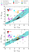 |
Fig. 12. Color-color diagrams of the potential host galaxies associated with FXTs 16, 18, 19, 20, 21 and 22 (colored stars), “distant” FXTs from Paper I (magenta hexagons), and X-ray sources classified as stars in Paper I (gray filled circles) and here according to Criterion 2 in Sect. 2.7.2 (black filled circles). The expected parameter space of stars with different ages [log(Age) = 7.0 − 10.3], metallicities ([Fe/H] = −3.0 − 0.5), and attenuations (AV = 0.0 − 5.0) taken from the MIST package (Dotter 2016; Choi et al. 2016) are overplotted as cyan regions. |
We further constrain the host properties through spectral energy distribution (SED) model fitting of their existing photometry using BAGPIPES (Bayesian Analysis of Galaxies for Physical Inference and Parameter EStimation; Carnall et al. 2018), which fits broadband photometry and spectra with stellar-population models taking star-formation history and the transmission function of neutral and ionized ISM into account via a MultiNest sampling algorithm (Feroz & Hobson 2008; Feroz et al. 2009). In Appendix C, we list the different conditions considered for the SED fitting. Table 6 provides the best-fit parameters obtained with BAGPIPES for the hosts of FXTs 16, 18, 19, 21 and 2229, while Fig. C.1 shows the 16th to 84th percentile range for the posterior spectrum, photometry, and the posterior distributions for five fitted host-galaxy parameters. Also, Figs. 13 and 14 compare the SFR and stellar masses of the FXT hosts to those of several well-known transient classes (such as CC- and Ia SNe, LGRBs, SGRBs and FRBs) and cumulative functions, respectively.
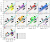 |
Fig. 13. Star-forming galaxy main sequence diagram, stellar mass vs. SFR, comparing hosts of FXTs and various other transient classes (one per panel) such as SNe type Ia, Ib, Ic, II (Tsvetkov & Bartunov 1993; Galbany et al. 2014; Schulze et al. 2021), super-luminous SNe (SL-SNe; Schulze et al. 2021), LGRBs (including SN 2020bvc; Chang et al. 2015; Li et al. 2016; Izzo et al. 2020; Ho et al. 2020), low-luminosity LGRBs (LL-LGRBs; GRB 980425, GRB 020903, GRB 030329, GRB 031203, GRB 050826, GRB 060218, and GRB 171205A; Christensen et al. 2008; Michałowski et al. 2014; Levesque 2014; Krühler et al. 2017; Wiersema et al. 2007; Wang et al. 2018; Arabsalmani et al. 2019), SGRBs (including GW 170817 or GRB 170817A; Li et al. 2016; Im et al. 2017; Nugent et al. 2022), TDEs (French et al. 2020), and Paper I FXT candidates (nearby and distant FXTs). Grayscale contours denote the SDSS galaxy distribution from Brinchmann et al. (2004). The solid cyan lines show the best-fit local galaxy main sequence relation from Peng et al. (2010), while the dashed colored lines denote the upward evolution of the boundary separating star-forming and quiescent galaxies as a function of redshift (at z = 0.0, 0.1, 0.2, 0.3, and 0.4; Moustakas et al. 2013). |
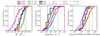 |
Fig. 14. Comparison of the host-galaxy properties of FXTs 16, 19, 21 and 22 (color vertical dashed lines) from Table 6 with the cumulative distributions of galaxy stellar mass (left panel), star-formation rate (center panel), and projected physical offset (right panel) for LGRBs (blue lines; Li et al. 2016; Blanchard et al. 2016), SGRBs (red lines; Fong et al. 2010, 2012, 2014, 2022; Margutti et al. 2012; Sakamoto et al. 2013; Berger et al. 2013b; Nugent et al. 2022), FRBs (black lines; Heintz et al. 2020), CC-SNe and Ia-SNe (cyan and orange lines; Tsvetkov & Bartunov 1993; Prieto et al. 2008; Galbany et al. 2014), and SLSNe (magenta lines; Schulze et al. 2021). |
Overall, in terms of stellar mass and star-formation rate, FXTs 16, 18, 19, and 22 are located above the galaxy main sequence, while FXT 21 lies slightly below it (see Fig. 13, solid cyan line). The hosts of FXTs 16, 19, and 22 have SFRs, stellar masses, and young stellar populations indicative of star-forming galaxies (Moustakas et al. 2013). In terms of SFRs, the FXT hosts broadly lie in the same region populated by SNe type Ib, Ic, II, SL-SNe, and GRBs. The SFR of the host of FXT 22 compares more favorably with LGRB (30%) and SGRB (10%) hosts over SNe (∼0%); meanwhile, its large host stellar mass shares little overlap with the LGRB/SGRB (≈10/15%) and partially with type-Ia/CC-SN (≈40/30%) host populations. For FXTs 16 and 19, the overlapping fractions of LGRB, SGRB, and SLSNe host galaxies with galaxy stellar mass ≲109 M⊙ are ≈20, 15, and 80%, respectively. In the particular case of FXT 18, it has a moderate SFR and low stellar mass. This low stellar mass matches with a very small fraction of LGRB (≲5%) and SGRB (≲2%) hosts and some SL-SNe (≈30%) hosts.
The host of FXT 21 has a moderate SFR and high stellar mass, implying a classification as a quiescent galaxy (Moustakas et al. 2013). Its SFR falls in a region populated by ≈70 and 50% of LGRBs and SGRBs, respectively, and ≈40 and 25% of CC-SNe and Ia-SNe hosts, respectively, with SFR ≳ 2.0 M⊙ yr−1. Meanwhile, only ≲10% of SNe and GRBs have similar host galaxy stellar masses ≳1011 M⊙.
Moreover, these sources fall in the same parameter space occupied by the distant FXTs reported in Paper I (see Fig. 13, lower panel). Thus, we conclude that a majority of distant FXTs appear to be associated with actively star-forming galaxies (≳108 M⊙ and ≳0.5 M⊙ yr−1), while a subset is associated with post-starburst (“green valley”) galaxies.
Another crucial parameter is the projected physical offset (δR) between the transient’s position and the host galaxy center. Figure 14, right panel, compares the projected physical offset distribution of FXTs 16, 18, 19, 21 and 22 to several transient classes such as CC-SNe (cyan), Ia-SNe (orange), SL-SNe (magenta), FRBs (black), LGRBs (blue) and SGRBs (red). SGRBs have a physical offset, which is about ∼4–5 times greater than the median offset for LGRBs (Bloom et al. 2002) and SL-SNe (Schulze et al. 2021), and about ∼1.5 times larger than the median offsets of CC- and Type Ia SNe (Prieto et al. 2008) and FRBs (Heintz et al. 2020). In addition, practically no LGRBs and SL-SNe, and only ≈10% of CC- and type Ia SNe have offsets ≳10 kpc, while ≈40% of SGRBs have such offsets. Moreover, ≈15% of SGRBs have offsets ≳20 kpc, while essentially no SL-SNe, CC- and type Ia SNe, or LGRBs exhibit such large offsets.
The physical offsets of FXTs 16 (≈3.3 kpc), 19 (≈3.9 kpc), and 21 (≈3.6 kpc) overlap with the cumulative distributions of CC- and type Ia SNe, and SGRBs at 1σ confidence level, although only ≈10−15% of SL-SNe and LGRBs have equal or higher offset values. In the case of FXT 18, its offset (≈13.2 kpc) resides well inside the offset distribution of SGRBs (≈70% with δR < 13 kpc), while just ≲5% of LGRBs, and CC- and Ia-SNe have equal or higher offset values. Nevertheless, it has a large X-ray positional uncertainty. In contrast, FXT 22 has a physical offset of ≈40 kpc, which is just compatible with ≈10% of SGRB hosts with equal or higher offsets.
5. Rates
We update the FXT event rates determined in Paper I and revisit comparisons with other transients to explore possible interpretations. Specifically, we derive the observed event rates (deg−2 yr−1; Sect. 5.1), FXT X-ray luminosity function (Sect. 5.2), and volumetric rates (yr−1 Gpc−3; Sect. 5.3).
5.1. Event-rate estimation
We compute FXT event rates following the procedure and assumptions outlined in Paper I (their Sect. 6.1 and Eqs. (5)–(7)). We first estimate the rate independently of Paper I to confirm consistency. We found eight FXTs inside ≈89 Ms of Chandra data from 2014 to 2022, yielding  deg−2 yr−1 (for sources with FX, peak ≳ 1 × 10⁻¹³ erg cm−2 s−1). This rate is consistent with the rates derived by Yang et al. (2019,
  ) and Paper I (
 deg−2 yr−1) at the Poisson 1σ confidence level and higher than the rate derived by Glennie et al. (2015, ≈3.4 deg−2 yr−1). As already mentioned in Paper I, this is not surprising since Glennie et al. (2015) computed the rate for a higher peak flux of FX, peak ≳ 1 × 10⁻¹⁰ erg cm−2 s−1. Then, considering all 17 distant FXTs (i.e., the nine distant FXTs from Paper I, also including the ambiguous FXTs 1 and 11 which might be extragalactic sources according to Eappachen et al. 2022, and the eight FXTs from this work) detected by Chandra (ACIS-I/S) instruments between 2000 and 2022, we estimate a total distant FXT event-rate of
  deg−2 yr−1. Since the number of FXTs removed erroneously by our selection criteria is ≪1 (see Sect. 2.7.6), the estimated event rates are robust results for FXT candidates brighter than FX ≳ 1 × 10⁻¹³ erg cm−2 s−1 (from the search algorithm developed in Paper I). Finally, we found no new local FXTs among the Chandra observations of nearby galaxies included in this work (i.e., 26.5% of the ObsIds), allowing a revised estimate (considering ObsIds from Paper I and this work) of the nearby FXT event rate of
  deg−2 yr−1, consistent with that derived in Paper I.
The event rate as a function of fluence (or peak flux30) behaves as a power-law function as  , where γ is a positive value.
Figure 15, left panel, shows the cumulative log𝒩–log S distribution of the entire sample analyzed in this work (i.e., 8 FXTs; orange line), FXTs identified in Paper I (i.e., 14 FXTs; cyan line), and finally combining both samples (i.e., 22 FXTs; black line) which appears to follow γ ≈ 0.5 (red region and line). We also plot the extrapolation of the best-fit slope, γ = 1.0, based on the estimates of FXTs at bright fluxes (≳10−10 erg cm−2 s−1) from Arefiev et al. (2003)31. The brightest sources in the total sample of 22 FXTs appear to be consistent with the Arefiev et al. (2003) extrapolation at 1-σ confidence. In contrast, the fainter sources fall well below it by ∼1 dex (following a power-law with an exponential index of γ = 0.52), indicating a break around a fluence of ∼10−8 erg cm−2 to our best-fit slope. A similar result was found in Paper I. Furthermore, we define a BPL model, which fits the results obtained (see Fig. 15), for the cumulative log𝒩–log S distribution with a break fluence around ∼1 × 10⁻⁸ erg cm−2 and two power-law indexes of γ1 = −0.52 and γ2 = −1.0 for the faint and bright ends, respectively.
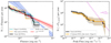 |
Fig. 15. Observed cumulative log𝒩–log S and log𝒩–log Fpeak distributions. Left panel: log𝒩–log S distribution of the sample of extragalactic FXTs analyzed in this work (orange line), from Paper I (cyan line), and combined (black line), as a function of fluence (in cgs units). Also shown are two PL models, N(> Fluence)∝S−γ, with slopes γ = 0.52 (red line) and 1.0 (blue dashed line). The γ = 1 line represents the best fit and 1σ error of Arefiev et al. (2003) based on bright FXTs (including Galactic flares). The brightest sources in our sample appear to be consistent with this bright-end extrapolation, although our fainter sources fall up to ∼1 dex below, implying a break. For comparison with Arefiev et al. (2003), we convert all FXT fluences to the 2−10 keV band from their best fits. Right panel: log 𝒩–log Fpeak distribution of the total sample of extragalactic FXTs analyzed in Paper I and this work (black line) and only distant FXTs (orange line). The magenta dashed line shows objects uniformly distributed in Euclidean space ( |

Finally, Fig. 15, right panel, represents the cumulative log𝒩–log Fpeak curves considering the whole sample of 22 FXTs (black line) and just the 17 distant FXTs for Paper I and this work (orange line). The local FXTs identified in Paper I contribute mostly to low fluxes (compare the orange and black lines). The log𝒩–log Fpeak slope appears to be significantly shallower at low Fpeak than the Euclidean prediction (i.e., ∝S−3/2, which is expected for astrophysical objects uniformly distributed in a Euclidean space; dashed magenta line). A combination of four effects could explain this deviation: (i) near the sensitivity threshold of the detector, the number of FXTs depends on the detection efficiency, which affects the log𝒩–log Fpeak plot; (ii) due to the flux being inversely proportional to the square of the luminosity distance, which will differ from the Euclidean distance as z approaches unity (this implies that the FXTs should be cosmological); (iii) the sample of FXTs likely has a mix of origins, such that the cosmic event rate density is not constant with redshift; and (iv) the sample is dominated by low-number statistical fluctuations, particularly at the bright end, due to the grasp (area × sensitivity) of Chandra. New X-ray missions which are focusing on scanning the sky, such as eROSITA and Einstein Probe, will increase the number of FXTs and improve our statistics.
5.2. Luminosity function
Past works have constructed X-ray luminosity functions (XLFs) for GRBs (Sun et al. 2015), SBOs (Sun et al. 2022), and TDEs (Sazonov et al. 2021). We construct here the XLF of FXTs considering distant sources from Paper I and this work, using the classical Vmax method from Schmidt (1968). We adopt the redshifts and peak X-ray luminosities shown in Table 9 (Cols. 2 and 3, respectively) and Fig. 16 (left panel), which also plots the limiting luminosity corresponding to a Chandra detection threshold of  erg cm−2 s−1 (green solid line; representing the conservative detection limit of our search algorithm) and 1 × 10⁻¹⁴ erg cm−2 s−1 (green dashed line; representing an approximate instrument threshold). All the FXTs except FXT 8 lie above
  erg cm−2 s−1.
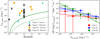 |
Fig. 16. Peak X-ray luminosity versus redshift and X-ray luminosity function of FXTs. Left panel: peak X-ray luminosity of FXT candidates from Paper I and this work (with known and fiducial redshifts; see Table 9). The green solid and dashed lines indicate peak flux limits of 10−13 (set by our algorithm) and 10−14 erg cm−2 s−1 (approximate Chandra on-axis detector limit), respectively. Right panel: FXT X-ray (0.3–10 keV) luminosity function (XLF) of the total sample from Paper I and this work. The red squares represent the XLF using the seven FXTs with known (photometric or spectroscopic) redshifts, while the blue and green squares show XLFs using all 17 FXTs with known+fiducial redshifts, adopting z = 1.0 and 0.5 for unknown objects, respectively. The solid lines show best-fit power-law models (see Table 10 for values). |
The XLF, Φ(L), is the sum of the individual contributions by each source (j) in the luminosity range from log(L) to log(L)+dlog(L) (with total ΔNL sources), that is,
![Mathematical equation: $$ \begin{aligned} \Phi (L)\ \mathrm{d}\log (L)=\sum _{j=1}^{\Delta N_{\rm L}}\frac{4\pi \ \mathrm{d}N(L)_j}{\left[\sum _{i=1}^{N_{\rm obs}}T_i\Omega _i V_{\mathrm{max},i}\right]_j}, \end{aligned} $$](/articles/aa/full_html/2023/07/aa45912-23/aa45912-23-eq155.gif) (3)
(3)
where i runs over the ith observation, Nobs is the total number of observations, Ti and Ωi are the exposure time and FoV per observation, respectively, Vmax, i is the maximum observable volume, and ΔNL is the total detectable number of sources.
Vmax for a given FXT in the sample depends on its intrinsic peak luminosity in the 0.3−10.0 keV energy band, which are both given in Table 9, assuming a flux limit of  erg cm−2 s−1 from our detection algorithm. To calculate the FXT XLF, we sum the derived
  values of individual FXTs in five equal 0.5 dex interval luminosity bins from log(LX, peak) between 44.0 and 47.5. The uncertainty within a given bin depends on the Poisson uncertainty of the number of FXTs per bin and Vmax (computed as
  , where the summation is done over the objects within that bin).
We estimate three different cases: (I) considering just eight FXTs with known redshifts, (II) considering 17 distant FXTs with known and fiducial (z = 1.0) redshifts, and (III) considering 17 distant FXTs with known and fiducial (z = 0.5) redshifts. The computed FXT XLFs are shown in Fig. 16 (right panel). In Case I (red squares), the largest uncertainties are associated with the lowest luminosity bins where there is just one FXT per luminosity bin. For Cases II and III (blue and green squares, respectively), the uncertainties are somewhat smaller because some luminosity bins have more than one source.
The FXT XLFs all appear to decline with increasing X-ray luminosity and are fit with power-law models as:
 (4)
(4)
The best-fit models are plotted in Fig. 16 as red, blue, and green lines for Cases I, II and III, respectively, with the results summarized in Table 10. Assuming fiducial redshifts of z = 1.0 (z = 0.5) naturally leads to shallower (steeper) XLF slopes.
Results of X-ray luminosity function (XLF) fitting.
Under the implicit assumption of no evolution, we can estimate the average FXT volumetric rate in the z ≈ 0 − 2.2 (see Table 9) Universe by integrating the XLF over the entire luminosity range used here (LX, peak > 1044 erg s−1). The results are tabulated in Table 10. For Case I, the average event rate density is ≈1.2 × 10³ Gpc−3 yr−1. Due to the total galaxy volume density of ∼2 × 10⁷ Gpc−3 (Bell et al. 2003), this equates to a rate of R ∼ 6 × 10⁻⁵ FXTs yr−1 per galaxy. On the other hand, considering the FXTs with known + fiducial redshifts of z = 1.0 (Case II) and z = 0.5 (Case III), the average FXT volumetric rates would be ≈1.3 × 10⁴ and ≈4.4 × 10⁴ Gpc−3 yr−1, respectively, implying rates of R ∼ 6.5 × 10⁻⁴ and 2.2 × 10⁻³ FXTs yr−1 per galaxy, respectively. The three derived FXT volumetric rates (which could be interpreted as a mean value for Cases I or II/III, respectively) remain consistent with previous results computed in Paper I (≈5 × 10³ Gpc−3 yr−1), Xue et al. (2019) (≈1.3 × 10⁴ Gpc−3 yr−1), and Bauer et al. (2017) (≳102 Gpc−3 yr−1 at z ≲ 1). Notably, these values differ by orders of magnitude from the rates computed previously for SMBH TDEs (≈210 Gpc−3 yr−1; Donley et al. 2002; Sazonov et al. 2021) and marginally with SBOs (≈4.6 × 10⁴ Gpc−3 yr−1; Sun et al. 2022) identified in eROSITA and XMM-Newton archival data, respectively. This further helps to exclude the SBOs (considering Case I) and SMBH TDE scenarios, although other transients may remain viable due to the large beaming correction uncertainties.
5.3. Volumetric density rate estimation
In Sect. 5.2, we estimated the average FXT volumetric rate in the redshift range z ≈ 0 − 2.2 from the XLF (see Table 10), assuming zero evolution. Now, we compare the volumetric density rate, in units of yr−1 Gpc−3, with other known transient classes such as GRBs, SBOs, or TDEs. First, because only eight of 17 distant FXTs have redshift estimates, we correct the FXT volumetric rate of Case I by the inverse of this fraction (i.e., multiply by 17/8) to account for the fact that we do not include all the sources. We implicitly assume here that the underlying redshift distribution of the sources without redshifts is the same as those with. Without this correction, the luminosity functions are lower limits rather than best estimates. Meanwhile, for Cases II and III, a correction factor is not necessary because both cases adopted fiducial redshifts (zfiducial = 1 and 0.5, respectively) for all FXTs that lacked estimates. Considering this correction, the volumetric density rate for Cases I, II and III ranges between ∼1.9 × 10³ − 4.6 × 10⁴ Gpc−3 yr−1 at 1σ confidence.
The derived density rate as a function of redshift is shown in Fig. 17 (gray filled region). Our result is consistent with the rates estimated in Paper I (≈4.8 × 10³ Gpc−3 yr−1 at zmax = 2.1; cyan circle) or CDF-S-XT2-like sources (purple square; Xue et al. 2019). Each panel in Fig. 17 represents a comparison with transients related to massive stars (LGRBs, LL-LGRBs, and CC-SNe; left panel), compact binary mergers (SGRBs; middle panel), and tidal disruption events (SMBH and IMBH TDEs; right panel).
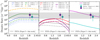 |
Fig. 17. Volumetric density rate as a function of redshift comparing FXTs (gray filled region, assuming no evolution with redshift and 1-σ confidence; see text for details) and other transients. Left panel: comparison to massive-star related sources such as CC-SNe (dashed orange line; |


As CC-SNe progenitors are massive, short-lived stars, the event rates should reflect ongoing star formation at different cosmological epochs (Madau & Dickinson 2014, and references therein). Thus to build the cosmic density rate shown in Fig. 17 (left panel), we use the star-formation history derived by Madau & Dickinson (2014), weighted by the number of stars that explode as SNe per unit mass  (Madau & Dickinson 2014), adopting a Salpeter initial mass function (orange-dashed lines).
One caveat for CC-SNe, however, is that we do not expect strong X-ray emission from all types of SBO CC-SNe. Thus, we analyze the expected rates for different subsamples of CC-SNe. The local event rate density of all CC-SNe types is ∼105 Gpc−3 yr−1 (see Fig. 17, left panel; Smartt et al. 2009; Li et al. 2011; Madau & Dickinson 2014). Around ∼59% of CC-SNe are Type II-P SNe from red supergiant star (RSG) progenitors. This means that the local rate of SBO from RSGs (which peak in the UV at a few eV; Alp & Larsson 2020; Sun et al. 2022) should be ∼6 × 10⁴ Gpc−3 yr−1, which is slightly higher than our result for FXTs (∼2 × 10³ − 4.5 × 10⁴ Gpc−3 yr−1). Meanwhile, around ≈1−3% of CC-SNe are Type II SNe from blue supergiant star progenitors (BSGs; Arnett et al. 1989; Pastorello et al. 2005), and ∼30% are Type Ib/c SNe from Wolf-Rayet star (WR) progenitors. SBOs from BSGs and WRs are expected to peak in the soft X-rays, 0.3 and 3 keV, respectively (Matzner & McKee 1999; Nakar & Sari 2010; Sapir et al. 2013). Thus, the local rates of SBOs related to BSGs and WRs are ∼2 × 10³ and ∼6 × 10² Gpc−3 yr−1, respectively. The derived event rate density of FXTs falls especially close to the expected rate of BSGs.
For LGRBs, we adopt a cosmic evolution rate following Sun et al. (2015), which we normalize to the local Universe value to characterize the cosmic density rate, as shown in Fig. 17 (left panel). LGRBs have an isotropic luminosity of ∼1049 − 1054 erg s−1, and an observed local density rate above 1050 erg s−1 of ρ0,LGRBs ∼ 0.5 − 1.0 Gpc−3 yr−1 (Zhang 2018). We additionally consider a jet beaming correction factor of  (blue-solid line), which corresponds to a mean jet opening angle
  (Frail et al. 2001). However, the beaming factor for LGRBs carries some uncertainties and various authors claim lower correction factors of ≈50−100 (blue-dotted and dashed lines, respectively; Piran 2004; Guetta et al. 2005). At z ≲ 0.6, the FXT volumetric rate exceeds the nominal LGRB rate by up to a factor of ∼7 (for the most favorable
  ), while they appear consistent beyond z ≳ 0.6. The FXT rate does not appear consistent with LGRB rates that adopt lower jet beaming correction factors (e.g.,
  or 100).
LL-LGRBs have relatively low isotropic luminosities of ∼5 × 1046 − 1049 erg s−1, limiting our ability to see them out to large distances, and hence comprise only a small fraction of observed LGRBs. As such, they have a much higher local density rate of ρ0,LL−LGRBs ∼ 100 − 200 Gpc−3 yr−1 (Zhang 2018), and generally do not show strong evidence of collimation, implying a much wider jet opening angle, or even that the emission is essentially isotropic, that is,  (Virgili et al. 2009; Pescalli et al. 2015). Normalizing the adopted cosmic evolution rate from Sun et al. (2015) to this value, we show the cosmic LL-GRB density rate as the green lines in Fig. 17 (left panel). Following Liang et al. (2007a), we also consider a LL-LGRB jet beaming correction factor of
  denoted by the green-solid line and the isotropic case (i.e.,
  ) denoted by the green-dashed line. The derived FXT volumetric rate is consistent with the more strongly beamed LL-LGRB rate, while it is slightly higher than lower beamed LL-LGRBs, especially at z ≳ 1.
For SGRBs, the cosmic density rate is then shown in Fig. 17 (middle panel), considering Gaussian (red lines), power-law (gray lines) and log-normal (purple lines) merger delay evolution models32, adopting an observed local density rate above 1050 erg s−1 of ρ0,SGRBs ∼ 0.5 − 3.0 Gpc−3 yr−1 (Wanderman & Piran 2015; Sun et al. 2015). Additionally, it is known that at least some short GRBs are collimated (Burrows et al. 2006; Soderberg et al. 2006; De Pasquale et al. 2010), with a mean jet opening angle  (e.g., Berger 2014; Fong et al. 2022; Rouco Escorial et al. 2022), translating to a mean value of
  (dotted lines; Fong et al. 2015). Nevertheless, the opening angle is not well-constrained, and other authors have suggested a wider range of
  (solid and dashed lines, respectively; Berger 2014; Fong et al. 2022; Rouco Escorial et al. 2022). From different delay models, we have distinct outcomes. For instance, from the delay merger Gaussian and log-normal models, the FXT volumetric rates between cosmic epochs z ≈ 0.8 − 2.0 appear slightly higher than the most extreme beaming correction case (
 ). In contrast, under the power-law model, the FXT volumetric rates are higher than even the most extreme beaming correction case.
Finally, in Fig. 17 (right panel), we consider both SMBH and IMBH TDEs, adopting the analytical cosmic density rate evolution of Sun et al. (2015). For SMBH TDEs, the model is normalized to the local value of ρ0, SMBH − TDE ∼ (0.7 − 1.4)×105 Gpc−3 yr−1 (magenta line; Sun et al. 2015). Moreover, we assume that IMBHs have grown in a similar way to SMBHs, and adopt same cosmic evolution, with a local density normalization of ρ0, IMBH − TDE ∼ 75 − 500 Gpc−3 yr−1 (cyan-dotted line; Malyali et al. 2019; Tanikawa et al. 2022). Like SMBH TDEs (e.g., Swift 1644+57; Bloom et al. 2011; Levan et al. 2011) and IMBH-WD TDEs could be capable of launching luminous jets which can be detected by current satellites, until reaching X-ray luminosities as large as ∼1048 erg s−1 (MacLeod et al. 2014, 2016). The FXT volumetric rate is generally lower than the rate of SMBH TDEs at z ≲ 0.8, while it matches with them at z ≳ 0.8. On the other hand, the FXT rate is much higher than our estimate of IMBHs, albeit with many untested assumptions (Malyali et al. 2019; Tanikawa et al. 2022). Of course, inconsistencies in several other parameters rule out an SMBH-TDE channel for several FXTs.
In Sect. 6, we use the volumetric rate of FXTs to understand the most likely progenitors of the different sources.
6. Possible interpretations
To assess the nature of our final sample of FXTs, we compare them with other well-known transients. For FXTs 16, 18, 19, 21, and 22, we adopt their best-fit photometric or spectroscopic redshifts in Table 6. For FXTs 15, and 17, which lack clear host associations in optical and NIR images, and 20, which only has three detections in DECam images and poor photometric redshift constraints, we assume a fiducial distance of z = 1, consistent with the average known redshift distribution. From the best-fit PL spectral model (see Table 7), we compute the peak X-ray flux (corrected for Galactic and intrinsic absorption; FX, peak), the associated intrinsic peak X-ray luminosity (LX, peak), and the Eddington mass (defined as MEdd = 7.7 × 10−39 LX, peak in solar mass units); values are reported in Table C.1 in the 0.3–10.0 keV band.
FXTs 16, 18, 19, 21 and 22 reach peak X-ray luminosities of LX, peak ≈ 2.8 × 1045, 1.9 × 1047, 3.7 × 1046, 6.9 × 1045 and 1.3 × 1046 erg s−1, and have isotropic energies of  , 1.7 × 1050, 1.3 × 1049, 1.8 × 1048, and 1.0 × 1049 erg, respectively (see Table C.1). Likewise, adopting z = 1, FXTs 15, 17, and 20 would have peak X-ray luminosities of LX, peak ≈ 1.0 × 1045, 6.3 × 1045 and 8.1 × 1046 erg s−1 and isotropic energies of
  , 3.4 × 1048, and 3.2 × 1048, respectively (see Table C.1). This luminosity range automatically excludes lower luminosity (LX, peak ≲ 1042 erg s−1) X-ray flaring transients such as X-ray binaries (including ultra-luminous X-ray sources), soft γ repeaters, quasi-periodic eruptions, and anomalous X-ray pulsars (e.g., Colbert & Mushotzky 1999; Kaaret et al. 2006; Woods & Thompson 2006; Miniutti et al. 2019). Below, in Sects. 6.1–6.3 we investigate the SBO, GRB, and TDE scenarios as origins of this FXT sample. In Sect. 6.4 we compare these FXTs with those identified in Paper I.
6.1. Supernova shock breakouts (SBOs)
One intriguing explanation for FXTs is related to the SBO from a CC-SNe. An initial flash of thermal UV or soft X-ray radiation is expected when a CC-SNe shock wave emerges from the stellar surface of the progenitor (Falk & Arnett 1977; Klein & Chevalier 1978; Matzner & McKee 1999; Schawinski et al. 2008; Ganot et al. 2016; Waxman 2017). The physical features of an SBO depend mainly on the density structure of the progenitor star and the explosion energy driving the shock wave (Chevalier & Irwin 2011; Gezari et al. 2015), which means that the temperature and duration of SBOs might cover a range of ∼105–5 × 10⁶ K and ≈100–5000 s, respectively (Ensman & Burrows 1992; Tominaga et al. 2011), leading to a bolometric peak luminosity of order ∼1044–1045 erg s−1. In the 0.5–7 keV band, we would expect to observe a soft thermal spectrum, potential spectral softening with time, and peak luminosities at least 1 dex lower than the bolometric values.
Until now, just one SBO has been detected conclusively in multi-wavelength observations, XRT 080109/SN 2008D, serendipitously discovered during Swift-XRT observations of SN 2007uy in NGC 2770 (Soderberg et al. 2008; Modjaz et al. 2009; Waxman 2017). Recently, a dozen further SBO candidates were reported among XMM-Newton archival data by Alp & Larsson (2020) and Novara et al. (2020). This subsample of FXTs has luminosities that fall within the ranges predicted by models and observations of SBOs ( –1044 erg s−1; Soderberg et al. 2008; Modjaz et al. 2009; Waxman 2017; Alp & Larsson 2020; Novara et al. 2020); however, at least four of these FXTs are associated with energy releases that are two orders of magnitude higher than SBO model predictions (e.g., Waxman 2017) or observations (e.g., XRT 080109/SN 2008D had EX ∼ 2 × 1046 erg; Soderberg et al. 2008).
Based on the energetics (the luminosity peaks are higher than those expected for SBOs,  erg s−1) and light curves (which are much brighter than the SBO XRT 080109/SN 2008D, see Fig. 18), we rule out an SBO origin for FXTs 16, 18, 19, 21, and 22. Due to the natural relation between SBOs and both CC-SNe and super-luminous SNe (SL-SNe), we expect them to share similar host-galaxy properties. The host properties of FXTs 16, 18, and 19 fall in regions populated by SNe type II and SL-SNe hosts, but lie at the edges of SNe type Ib and Ic host distributions (see Fig. 13). FXTs 21 and 22 reside at the edges of the SNe type Ib, Ic, and II, and outside the SL-SNe host distributions (see Fig. 13). Thus, the FXT hosts do not show a robust link with SNe host galaxies, reinforcing the previous results from the energetics.
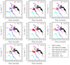 |
Fig. 18. Light curves of the eight FXTs in 0.3–10 keV luminosity units (converted from 0.5–7 keV light curves assuming best-fit spectral models in Sect. 3.3). Several individual transients are overplotted: XRF 080109/SN 2008D (the low-luminosity supernova SBO; solid cyan lines, 27 Mpc); XRF 060218/SN 2006aj (solid blue lines, 145 Mpc); XRF 100316D/SN 2010bh (solid orange lines, 263 Mpc; Barniol Duran et al. 2015; Starling et al. 2011; Modjaz et al. 2009; Evans et al. 2009, 2007; Soderberg et al. 2008; Campana et al. 2006); GRB 110328A or Swift J1644+57 (relativistically beamed TDE; solid black lines, z = 0.3543; Bloom et al. 2011; Levan et al. 2011); J2150−0551 (unbeamed TDE; solid pink line, z = 0.055; Lin et al. 2018). For FXTs 15, 17, 18 and 20 (open symbols), we assume z = 1.0, and for FXTs 16, 19, 21, and 22 we take the redshift values from Table 6. |
Similarly, for the FXTs which lack hosts (15, 17) or redshift (20), the SBO scenario is ruled out at the fiducial z = 1 values. The sources would need to lie at redshifts of z ≲ 0.37, 0.10, and 0.05, respectively, to comply with the expected energetic limits. At these redshifts, the apparent r-band magnitudes or limits would imply hosts with Mr ≳ −18.5, −15.9, and −13.0, respectively; only the host of FXT 15 lies at the faint end of regular galaxies, while the rest fall in the broad range of dwarf galaxies. FXTs 15 and 20 have BPL light curves with break times at ≈3.7 and 0.1 ks, respectively, followed by PL decays, FX ∝ t−2.7, that are accompanied by possible softening (see Table 8) and photon indices (Γ = 2.1 and 3.0, respectively; see Table 7), similar to the SBO XRF 080109/SN 2008D (Γ ≈ 2.3; Soderberg et al. 2008). Finally, we note that contemporary optical time domain surveys would have detected an observable SNe associated with FXTs 17 and 20, if they were at z ≲ 0.1. In summary, we do not find evidence in support of an SBO origin for FXTs 17 or 20, but cannot discard it completely for FXT 15.
Comparing the FXT rate with the much larger total CC-SNe rate, it is clear that only a small fraction of SBOs can lead to FXTs (see Fig. 17, left panel). After analyzing the volumetric rate of different massive star progenitors, we conclude that just some stars are more consistent with FXTs (see Sect. 5.3). Although the derived event rate density of FXTs falls especially close to the expected rate of BSGs (∼2 × 10³ Gpc−3 yr−1), such an association is largely ruled out by other characteristics such as energetics and host-galaxy properties. Thus, we conclude that this sample of FXTs is unlikely to be associated with SBOs from normal CC-SNe.
6.2. Gamma-ray bursts (GRBs)
GRBs are characterized by an average emission timescale of ≈20 s for LGRBs and ≈0.2 s for SGRBs (Meegan et al. 1996; Mészáros 2006). Currently, the accepted model of GRBs consists of a relativistically expanding fireball with associated internal and external shocks (Mészáros & Rees 1997). Once the γ-ray emission is generated, the expanding jetted fireball interacts with and shocks the surrounding interstellar medium, producing a broadband X-ray-to-radio afterglow. When the Doppler boosting angle of the decelerating fireball exceeds the jet aperture angle, it produces a steepening in the light curve known as the “jet break” (Sari 1999; Rhoads 1999; Zhang & Mészáros 2004). The majority of LGRBs arise from the core-collapse of massive stars associated with hydrogen-poor, high-velocity type Ic supernovae (Hjorth et al. 2003; Cano 2013; Levan et al. 2016). On the other hand, the current model of SGRBs is linked to the merger of a compact NS–NS or NS–BH binary (e.g., Eichler et al. 1989; Narayan et al. 1992), induced by angular momentum and energy losses due to gravitational wave (GW) emission and leading to a GW burst (Abbott et al. 2016). The NS–NS channel could produce as a remnant either a millisecond magnetar (e.g., Zhang 2013; Sun et al. 2017) or a BH surrounded by a hyper-accreting debris disk. The NS–BH channel may also generate a debris disk, if the NS is disrupted outside the BH event horizon by tidal forces (Rosswog 2007; Metzger 2019). Once it happens, both the high accretion rate and rapid rotation yield energy extraction, thus allowing the launching of a relativistic jet, via either neutrino-antineutrino annihilation or magneto-hydrodynamic processes (e.g., Blandford & Znajek 1977; Rosswog & Ramirez-Ruiz 2002; Lee & Ramirez-Ruiz 2007). The accretion event could produce an isotropic thermal supernova-like emission on timescales of ≈104–106 s called “kilonova” (e.g., Berger et al. 2013a; Tanvir et al. 2013; Gao et al. 2015; Sun et al. 2017; Pian et al. 2017; Arcavi et al. 2017; Metzger 2019).
No contemporaneous γ-ray counterparts are detected near the X-ray trigger times for any FXTs in our sample, ruling out an on-axis GRB scenario. The intrinsic light curves of all FXTs, except 18, are flatter and fainter than the vast majority of on-axis X-ray afterglows over the same timescales (2D shaded histogram in Fig. 19), with initial luminosities ≈1−2 dex below the luminosity range  erg s−1 observed for GRBs. Beyond ∼102–103 s, however, most FXTs do begin to overlap energetically with the low-luminosity on-axis X-ray GRB afterglows.
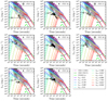 |
Fig. 19. Similar to Fig. 18. The X-ray afterglow light curves of 64 LGRBs plus 32 SGRBs (taken from Bernardini et al. 2012; Lü et al. 2015) are shown as a 2D histogram, while several individual transients are overplotted: GRB 111209A (ultra-long duration LGRB; solid magenta line, z = 0.677; Levan et al. 2014); GRB 170817A (off-axis SGRB, multiplied by ×1000; solid dark green line; Nynka et al. 2018; D’Avanzo et al. 2018; Troja et al. 2020, 2022); SN 2020bvc (the first off-axis LGRB candidate; solid light green line; Izzo et al. 2020), and theoretical off-axis GRB afterglows at different viewing angles θobs (solid and dashed colour lines represents afterglows with isotropic-equivalent energy and circumburst density of 1053 erg, 1 cm−3 and 1051 erg, 0.15 cm−3, respectively; Berger 2014; Ryan et al. 2020; Chrimes et al. 2022). For FXTs 15, 17, 18, and 20 (open symbols), we assume z = 1.0, and for FXTs 16, 19, 21, and 22, we take the redshift values from Table 6. |
Overall, GRBs have canonical light curves which can be split into up to five different components (Zhang et al. 2006), although not all X-ray afterglows necessarily exhibit all of them (e.g., Nousek et al. 2006; Willingale et al. 2007; Zhang et al. 2007; Evans et al. 2007, 2009; Liang et al. 2007b, 2009). The light curves components are (from the earliest to the latest): (i) steep decay phase (it is the tail of the prompt emission, from FX ∝ t∼ − 3 to ∝t∼ − 10); (ii) shallow decay or plateau phase (it could be interpreted invoking a continuous energy injection by a central engine, from FX ∝ t∼ − 0.7 to ∝t∼0.0); (iii) normal decay phase (it is the typical value predicted in the standard external forward shock model, FX ∝ t∼ − 1); (iv) jet break phase (it is a geometrical effect, FX ∝ t∼ − 2); and (v) X-ray flares (the GRB central engine directly powers them).
We note that FXTs 17, 18, and 21 exhibit PL decay light curves, similar to the normal decay phase of GRBs, while the other FXTs follow BPLs. However, FXTs 17, 18, and 21 as FX ∝ t−0.3 and ∝t−0.5, which is much shallower than the characteristic normal and jet-break phases (Evans et al. 2009, 2007; Racusin et al. 2009), but could be consistent with a shallow decay or plateau phase (Troja et al. 2007; Rowlinson et al. 2010). Notably, FXT 21 exhibits temporal flaring behavior, which is potentially comparable to the strong X-ray flaring episodes seen in the tails of the X-ray afterglow in some GRBs (Barthelmy et al. 2005; Campana et al. 2006; Chincarini et al. 2010; Margutti et al. 2011), while its best-fit X-ray spectral slope of ΓFXT 21 = 3.1 ± 0.6 is consistent with that of the standard afterglow distribution (ΓGRBs = 1.5 − 3.0; Berger 2014; Wang et al. 2015; Bauer et al. 2017) at the 1σ confidence level.
On the other hand, FXTs 16, 19, and 22 show light curves consistent with a ≈2.1–3.7 ks plateau phase followed by a power-law decay (FX ∝ t−1.9/−3.0; see Fig. 8 and Table 5) accompanied by likely spectral softening, especially for FXT 16 (see Fig. 8 and Table 11). Spectral softening has been seen previously in some GRBs afterglows (e.g., GRB 130925A; Zhao & Shao 2014). FXTs 16, 19 and 22 have photon indices (Γ ≈ 2.1 − 2.3; see Table 7) similar to GRB afterglows (ΓGRBs ≈ 1.5 − 3.0; Berger 2014; Wang et al. 2015). Notably, some subsets of LGRBs (e.g., Lyons et al. 2010) and SGRBs (e.g., Rowlinson et al. 2010, 2013; Gompertz et al. 2014) exhibit plateau phases, although only < 10% have plateau luminosities ≲1047 erg s−1 which would be consistent with FXTs 16, 19 and 22 at their redshifts.
Finally, FXTs 15 and 20 have BPL light curves with break times at ≈3.7 and 0.1 ks, respectively, followed by PL decays, FX ∝ t−2.7, accompanied by possible softening (see Table 8) and photon indices (Γ = 2.1 and 3.0, respectively; see Table 7) similar to GRB afterglows (Γ ≈ 1.5 − 3.0; Berger 2014; Wang et al. 2015) at a 1σ confidence level. However, their early rise phases (FX ∝ t0.4 and ∝t1.0 for FXTs 15 and 20, respectively, see Table 5) are incongruent with the typical decays of on-axis GRBs X-ray afterglows (from  to ∝t−2.0). FXT 20’s light curve shows many similarities to FXT 14 or CDF-XT1 (see Fig. D.1), where its X-ray luminosity reaches a value of
  erg s−1 without a clear softening in the spectra. The nature of FXT 14/CDF-XT1 is still unknown, although several scenarios have been proposed recently by Sun et al. (2019), Peng et al. (2019) and Sarin et al. (2021).
We introduce the option of FXTs being associated with X-ray flashes (XRF), which may be related to shock breakout from choked GRB jets (see Fig. 18; Campana et al. 2006; Bromberg et al. 2012; Nakar & Sari 2012). We compare the light curves of the XRF 060218/SN 2006aj (Pian et al. 2006; Campana et al. 2006) and XRF 100316D/SN 2010bh (Starling et al. 2011) related with LL-LGRBs. We note that the plateau phases of FXTs 16, 19, and 22 have similar luminosities to those of XRF 060218 and XRF 100316D (LX, peak ∼ 1045–1046 erg s−1), and the break and late-time light curves also appear to match reasonably well. FXT 18 has higher luminosities (≈1047 erg s−1) at early times than XRF 060218 and XRF 100316D, but it matches with them at later times. On the other hand, FXT 21, with its known redshift, looks inconsistent by a factor of ≳5 compared to the XRFs khown. Finally, the light curves of FXTs 15, 17, and 20 could be consistent with those of XRFs, but the lack of constrained redshifts does not permit a proper intrinsic comparison of energetics. Importantly, XRF 060218 and XRF 100316D show significant soft thermal components (kT ∼ 0.1 − 0.2 keV) which become dominant beyond ∼1000 s (Campana et al. 2006; Starling et al. 2011; Barniol Duran et al. 2015). We find that only FXT 16 shows comparable spectral behavior; FXTs 15, 19, 20, and 22 do not exhibit any similar robust trend while FXTs 17, 18, and 21 actually appear to marginally harden at late times.
We also consider the option of FXTs being off-axis components of GRB afterglows (see Fig. 19). To explore this scenario, we use a numerical model, called afterglowpy (developed by Ryan et al. 2020), to calculate synthetic light curves in X-rays. We generated synthetic X-ray afterglow for a range of viewing angles (from 0 to 8.6 deg) and assuming an isotropic-equivalent energy of 1053 (1051) erg and a circumburst density of 1.0 (0.15) cm−3, respectively (Fig. 19, solid [dashed] lines), which represent the typical parameters for LGRBs (SGRBs) (e.g., Berger 2014; Chrimes et al. 2022, and references therein). For instance, LGRBs and SGRBs occur in high- and low-density environments, respectively, while SGRBs are less energetic than LGRBs33. The light curves have a rise (from ∼1 to 104 s, see Fig. 19) before reaching a peak luminosity, followed by an afterglow consistent with the on-axis GRB trend. Figure 19 shows that an off-axis afterglow under small viewing angles could match the light curves of FXTs 15 and 20. In contrast, sources such as FXTs 16, 19, and 22, which have a plateau phase, cannot match the expected fast rise and curvature at early times of the slightly off-axis GRB cases. On the other hand, the light curves of some FXTs do appear to crudely match certain off-axis angle cases of SGRBs (dashed lines), because of their lower luminosity. Finally, we compare FXTs with the potential high inclination off-axis LGRB SN 2020bvc (with viewing angle θobs ≈ 23 deg; Izzo et al. 2020), and SGRB GRB 170817A (with viewing angle θobs ≈ 23 deg; Nynka et al. 2018; D’Avanzo et al. 2018; Troja et al. 2020, 2022) in Fig. 19. Notably, SN 2020bvc and GRB 170817A are much less luminous (LX, peak ≲ 3 × 1041 erg s−1) than the sample of FXTs, by at least ∼5 orders of magnitude. In general, at high off-axis angles, we can expect later onsets, fainter light curves, lack of decay phases at early times, and peak luminosities at later times (e.g., Granot et al. 2002; Ryan et al. 2020; Oganesyan et al. 2020; Ascenzi et al. 2020). Overall, this comparison suggests that an association of FXTs with high inclination angle afterglows of GRBs is unlikely, although a mildly off-axis SGRB scenario remains plausible.
In terms of host galaxies (see Sect. 4 for more details), based on the host stellar mass and SFR of FXTs 16, 18, 19, and 22, the galaxies lie above the galaxy-main sequence, in a parameter-space region populated mainly by GRBs (see Fig. 13). Nevertheless, it remains difficult to disentangle an association with LGRBs or SGRBs from the current data. In contrast, FXT 21’s host is below the galaxy-main sequence and shares properties more similar to SGRB hosts (especially the stellar mass).
Due to the physical offsets of FXTs 16, 19, and 21 (Fig. 14, right panel) overlapping with the cumulative distributions of CC- and type Ia SNe, and SGRBs at 1σ confidence level (see Fig. 14), the projected physical offsets are not enough to confirm or rule out the different scenarios. Although the offset distance of FXT 18 suggests a unique and apparent association with SGRBs, the considerable associated X-ray positional uncertainty does not permit us to consider its offset as a robust discriminator. Finally, FXT 22 has a sizeable physical offset which strongly disfavors a robust association with LGRBs, CC-, type Ia SNe, leaving only a SGRB association as a possible scenario. For instance, the dynamical evolution of the BNS due to a kick velocity (the formation of each compact object is associated with one supernova explosion; Fong & Berger 2013; Berger 2014, and references inside) could explain the significant offset of FXT 22 (≈40 kpc).
In the case of FXT 16, its light curve (the plateau and power-law decay as FX ∝ t−2), spectral softening trend, host-galaxy offset distance, and host-galaxy properties are consistent with a compact star merger origin, following Xue et al. (2019). Sun et al. (2019) explain the X-ray emission assuming a magnetar remnant after a BNS merger observed at a slightly off-axis viewing angle. Although FXTs 19 and 22 do not follow the same spectral trend, they share similar timing properties (a plateau phase in their light curves) and belong to star-forming host galaxies, as does FXT 16. However, FXT 22’s host is one of the most massive galaxies of the sample.
The volumetric rates reinforce some previous conclusions from the timing, spectra, and host properties (for more details, see Sect. 5.3). In the case of LGRBs (see in Fig. 17, left panel), the FXT volumetric rate is higher than the LGRB rate by up to a factor of ∼7 at z ≲ 0.6 (even for  ), but appears consistent beyond z ≳ 0.6 just for the case
  . In this sense, LGRBs with higher beaming corrections remain a potential progenitor for FXTs, while an association with LGRBs with lower jet beaming factors (e.g.,
  ) seems unlikely. However, the lower luminosity of FXTs becomes challenging to explain under this context. Moreover, we identified that the FXT volumetric rate is well-matched to the LL-LGRB rate considering a moderate beaming correction (
 ), while it is slightly higher than lower beamed LL-LGRBs (
 ) beyond z ≳ 1 (see Fig. 17, left panel). Thus, based on volumetric rates and luminosities, we conclude that LL-LGRBs remain a viable channel to explain FXTs. However, host properties do not align completely with this statement.
Finally, in the case of SGRBs, the volumetric rates give possible clues about an association between FXTs and SGRBs. From the delayed merger Gaussian and log-normal models, the FXT volumetric rates at z ≳ 0.8 and z ≲ 2 appear slightly higher than even the case of  (see Fig. 17, middle panel). Meanwhile, FXT remains a factor of ∼4 higher than SGRB rates assuming lower beaming correction values (i.e.,
  ). Thus, a link with SGRBs remains plausible, although it requires relatively strong beaming corrections, which unfortunately remain poorly constrained. This result agrees with the low luminosity of FXTs and the host galaxy properties.
6.3. Tidal disruption events
Another potential FXT progenitor scenario is related to TDEs (Rees 1988; Phinney 1989; Burrows et al. 2011; Saxton et al. 2021). TDEs occur when a red giant (RG), main-sequence (MS) star or WD (≈0.008−0.02 R⊙; ≈1 M⊙) passes so close to a SMBH or IMBH that it undergoes tidal forces which exceed its self-gravity, causing it to be disrupted. A substantial fraction of the tidal debris will fallback onto the BH, leading to luminous thermal emission at soft X-ray through optical wavelengths, either by the accretion of this gas onto the BH and/or the initial shocks due to colliding stellar debris streams (Guillochon & Ramirez-Ruiz 2015). A delay between the disruption and the accretion of gas onto the black hole may cause a delay between the optical and X-ray emission (e.g., Hayasaki & Jonker 2021). The debris fallback rates can range from strongly (∼104) super-Eddington to strongly (∼10−3) sub-Eddington, with respective peak timescales from < 1 day to more than 100 years (e.g., Law-Smith et al. 2017). This is confirmed by an observed empirical correlation between the peak light curve emission time and IMBH and SMBH mass (van Velzen et al. 2020), such that IMBH-WD TDEs are expected to rise to peak within minutes/hours, while SMBH/IMBH-MS TDEs (depending on the mass and spin) take roughly months to years (Krolik & Piran 2011; Haas et al. 2012; Kawana et al. 2018).
For MS stars disrupted by a SMBH (106–108 M⊙) or IMBH (103–105 M⊙), the radiation should peak around Teff ∼ 104 − 106 K, that is, at UV to soft X-ray wavelengths. Mild cooling is predicted, although substantial variations are seen empirically (Gezari 2021). For BHs exceeding ∼105 M⊙, a WD would be swallowed whole, leaving no expected emission signature (Clausen et al. 2012; Kawana et al. 2018). However, a high spin rate that increases the Hills mass for BHs with masses ≲106 M⊙ could enable IMBHs to potentially disrupt more white dwarfs, but, overall, it is difficult to explain all the X-ray flares as solely due to WD TDEs (Maguire et al. 2020). In addition to the possibility of exceeding the Eddington rate by large factors, emission from relativistic jets is also possible, particularly if the disruption involves a strongly magnetic WD (e.g., Cenko et al. 2012; Brown et al. 2015; Sądowski et al. 2016). Relativistic beaming from jetted TDEs such as Swift J1644+57 (black solid lines in Fig. 18; Bloom et al. 2011; Levan et al. 2011; Saxton et al. 2021) can generate much higher luminosities (LX, peak ∼ 1048 erg s−1), rapid and strong variability, and harder X-ray spectra (Γ = 1.6 − 1.8; Levan et al. 2011), although the photon index softens with decreasing flux (Bloom et al. 2011). However, some sources, such as the TDE AT2021ehb, show a hardening spectral trend with time, which is interpreted as the gradual formation of a magnetically dominated corona (Yao et al. 2022).
TDEs involving SMBHs should occur in the centers of more massive galaxies. Thus, we can automatically discard an association of FXTs 16, 19, 20, and 22 with SMBH TDEs because the sources are offset from the centers of their host galaxies. In the case of FXT 18, although it is offset from its host galaxy candidate, the significant X-ray positional uncertainty does not allow us to rule out the association with SMBH TDEs. We arrive at a similar conclusion for FXT 21 and the hostless events FXTs 15 and 17. In contrast, TDEs involving IMBHs may occupy a larger range of possibilities, for instance, occurring near the centers of dwarf galaxies or in crowded stellar systems such as globular clusters (e.g., Jonker et al. 2012; Reines et al. 2013). Thus, the offset of FXTs 16, 19, 20, and 22 remain consistent with a possible IMBH-WD TDE association. Moreover, given the short durations of the FXTs and exclusive detection in the X-ray band to date, the IMBH-WD TDE scenario seems to be most applicable. Below, we explore the association with IMBH TDEs.
The BPL light curves of FXTs 15 and 20 most closely follow the expected light curve shape for IMBH–WD TDE candidates (e.g., MacLeod et al. 2014; Malyali et al. 2019; Peng et al. 2019), with a fast rise and exponential decline (see Fig. 8 and Table 5). Although their late-time spectral slopes are relatively soft, their initial slopes are much harder than expected for TDEs (Tbbody ≈ 0.02 − 0.13 keV; Gezari 2021). The nominal peak luminosities of LX, peak ∼ 1045–1047 erg s−1, respectively, at fiducial redshifts of z = 1, are several orders of magnitude larger than the expected Eddington limits for IMBH-WD TDEs or what is observed from local candidates (e.g., IMBH TDE candidate TDE J2150–05 has a LX, peak ∼ 1043 erg s−1; Lin et al. 2018), requiring invocation of extreme super-Eddington accretion or relativistic beaming to explain them under a TDE scenario. The peak luminosities are more in line with beamed TDEs Swift J1644+57 (LX, peak ∼ 1046–1048 erg s−1; see Fig. 18; Bloom et al. 2011; Levan et al. 2011), but it is related with an SMBH TDE emission (although some authors claim by an association with IMBH TDEs, e.g., Krolik & Piran 2011). We cannot exclude an IMBH TDE explanation for FXTs 15 and 20, although they would clearly require special conditions.
FXTs 17, 18, and 21 show PL declines from the very start with relatively soft spectral slopes. The lack of any detectable rise appears inconsistent with expected TDE light-curve shapes. However, the soft X-ray spectral shapes, particularly in the case of FXT 18, are potentially consistent with the properties of some IMBH TDEs (e.g., MacLeod et al. 2014; Malyali et al. 2019). Moreover, we do not have sufficient counts to resolve the fast rise times which it may expect for some IMBH-WD TDEs (e.g., MacLeod et al. 2016). Again, the peak luminosities (adopting a fiducial redshift of z = 1 and photometric redshift of 0.35 for FXTs 17 and 18, respectively) are a few orders of magnitude larger than the expected Eddington limits for IMBH-WD TDEs or what is observed from local candidates, requiring super-Eddington accretion or relativistic beaming to explain them under an IMBH TDE scenario. Subsequent observations for FXT 17 can rule out any extended bright, long-term variability, however, it is not the case for FXT 18, which has not been revisited by X-ray observatories. For these reasons, we disfavor a TDE explanation for FXTs 17 and 21.
The light curves of FXTs 16, 19, and 22 show ≈2.1–3.7 ks plateaus with subsequent power-law decay (from FX ∝ t−1.9 to ∝t−3.0), accompanied by robust spectral softening in the case of FXT 16 (Fig. 8, and Tables 5 and 11). Although not commonly observed in X-ray emission from TDEs as yet (Gezari 2021), some eccentric fallback or reprocessing scenarios could potentially explain this behavior. On the other hand, the overall spectra of FXTs 16, 19 and 22 are best-fit with photon indices of Γ ≈ 2.1 − 2.3 (see Table 7), which are much harder than expected for TDEs, while their peak luminosities (LX, peak ≈ 3 × 1045–7 × 1046 erg s−1) are also generally much higher than candidate IMBH-TDEs identified to date. A relativistic-beamed IMBH-TDE scenario could better explain some of the X-ray properties (luminosities, spectral slopes) of FXTs 16, 19, and 22 (e.g., Peng et al. 2019 argue for an IMBH–WD TDE scenario for FXT 16), although subsequent observations indicate that none shows extended durations or variability evolution such as seen in Swift J1644+57. Finally, FXTs 16, 19, and 22 are all significantly offset from the nuclei of their associated hosts by  (or physical distances of ≈3.3–40 kpc; see Fig. 6), requiring an ejected IMBH scenario, or in the stripped nucleus of an infalling galaxy (such as TDE J2150–05; Lin et al. 2018), in order for the TDE scenario to remain viable. For these reasons, we disfavor a TDE explanation for FXTs 16, 19, and 22, although relativistically beamed emission from an IMBH–WD TDE scenario cannot be ruled out.
Regarding the host galaxy properties, we might expect to find IMBHs near the centers of dwarf galaxies, in globular clusters at large offsets in massive galaxies, or ejected via 3-body interactions (Komossa & Merritt 2008; Jonker et al. 2012; Reines et al. 2013). This, we might naively expect to identify FXTs associated with IMBH-WD TDEs in any type of host galaxy, and with a wide range of projected offsets. FXTs 16, 18 and 19 have hosts with M* ≲ 109 M⊙, while FXT 21 and 22 hosts have larger stellar masses (M* ∼ 1011 M⊙). Thus, we cannot discard an IMBH-WD TDEs scenario for FXTs for any event.
FXTs rate is only lower than the rate of SMBH TDEs for z ≲ 0.8 (see Fig. 17, right panel). In contrast, in the case of IMBH-TDEs, the FXT rate is much higher during the cosmic time but potentially consistent with just a fraction of FXTs (because likely we have a mix of FXTs origins). Another possibility could be the different energetics between FXTs and IMBH TDEs (discarding the beaming case, which occurs just in a small fraction of events). Moreover, based on inconsistencies in several other parameters (such as the offset from transient X-ray position and host galaxies) we can rule out an SMBH-TDE channel for several FXTs.
Finally, the partial consistency between volumetric rates of FXTs and different transients classes at different redshifts (see Sect. 5 for more details), timing and spectral parameters (see Sect. 3), and host properties (see Sect. 4), may suggest that the overall sample of FXTs arise from a heterogeneous set of progenitors. Detection of contemporaneous EM counterparts from future FXTs remains crucial to disentangle these multiple formation channels. Nonetheless, we strongly caution the reader not to overinterpret the consistency or lack thereof between FXTs and many of the transient classes, as we have implicitly assumed no density evolution in our calculations (which there easily could be) and the density evolution assumed for several of the other transient classes is not well-constrained. Thus, some of the previously mentioned discrepancies at low or high redshift could be no more than artifacts of these assumptions.
6.4. FXTs discovered in Paper I
The FXTs discovered here share many similarities with the previous distant FXTs identified in Paper I, in terms of their timing (Fig. D.1), spectral (Figs. 10 and 11), and host-galaxy properties (Fig. D.2). Unfortunately, the lack of host-galaxy detections for many FXTs identified here and in Paper I does not permit more detailed comparisons of energetics among the two samples. It is clear that according to the properties of the hosts we do detect, there is no single unifying class of galaxies (in terms of SFR and stellar mass) that could harbor a unique kind of transient. We conclude that the FXTs reported here likely have z ≳ 0.2, that is, they are not related to local galaxies (see Fig. D.2, bottom panel), and presumably span a wide distance range.
7. Expected sources in current and future missions
Based on the event rate computed in Sect. 5.1, we explore the expected number of FXTs that should be detectable in other ongoing and future X-ray missions. The expected event rate of another (New) mission (called ℛNew) regarding our results (ℛTotal) is
![Mathematical equation: $$ \begin{aligned} \mathcal{R} _{\rm New} = \left[\frac{\mathcal{N} ({>}S_{\rm New,lim})}{\mathcal{N} ({>}S_{\rm CXO,lim})}\right]\mathcal{R} _{\rm Total}, \end{aligned} $$](/articles/aa/full_html/2023/07/aa45912-23/aa45912-23-eq192.gif) (5)
(5)
where ℛNew and 𝒩(> SNew, lim) are the event rate and X-ray fluence limit of the new mission (taken from Sect. 5.1), respectively, and 𝒩(> SCXO, lim) represents the fluence limit of Chandra (taken from Sect. 5.1). As we explain in Sect. 5.1, the event rate behaves as a BPL function. Then, the expected total number of sources must be
![Mathematical equation: $$ \begin{aligned} \mathcal{N} _{\rm New}&= \Omega _{\rm New} T_{\rm New} \mathcal{R} _{\rm New} \times \frac{\mathrm{EA}_{\rm New}}{\mathrm{EA}_{\rm CXO}}\nonumber \\&=\Omega _{\rm New} T_{\rm New}\left[\frac{\mathcal{N} ({>}S_{\rm New,lim})}{\mathcal{N} ({>}S_{\rm CXO,lim})}\right]\mathcal{R} _{\rm Total}\times \frac{\mathrm{EA}_{\rm New}}{\mathrm{EA}_{\rm CXO}}, \end{aligned} $$](/articles/aa/full_html/2023/07/aa45912-23/aa45912-23-eq193.gif) (6)
(6)
where ΩNew and TNew are the FoV and the operational time of a new mission, respectively. Also, we consider an ad hoc term, EANew/EACXO, which is a correction factor defined as the ratio between the integrated effective area of the new mission and Chandra in the energy range of 0.5−7.0 keV34. It is important to realize that Eq. (6) considers the ratio between the new mission (FNew, lim) and Chandra (the limit imposed by our method FCXO, lim = 1 × 10⁻¹³ erg cm−2 s−1, which is roughly 10× the nominal point source detection sensitivity in a 10 ks window; see Sect. 2.1 in Paper I) X-ray flux limits, respectively. We estimate numbers adopting a limit 10× above the new mission’s nominal 10-ks flux limit to avoid the Poisson fluctuations in our calculations. Given the low-count statistics, we quote estimates incorporating the Poisson 1σ errors.
We begin with estimates for ongoing missions (XMM-Newton, Swift-XRT, and SRG-eROSITA), and then future observatories (Athena, Einstein Probe, STAR-X and AXIS) which are expected to have enough flux sensitivity and time in orbit to detect similar FXTs as those found here. Table 11 shows a summary of the assumed FoV, Tnew and Fnew, lim used to calculate the expected number of FXTs per year for each mission and our results; we give the expected number of FXTs per year to allow the reader to compute more readily the number of FXTs for any exposure time or mission length given. For all missions, we adopt a spectral slope of Γ = 1.7 − 2.3, typical of FXTs. More accurate estimates involving Monte Carlo techniques go beyond the scope of this work.
Expected number of FXTs for different X-ray missions.
The European Photon Imaging Camera (EPIC) on board the XMM-Newton telescope has a FoV ≈ 0.25 deg2, 10-ks flux sensitivity of ≈10−14 erg cm−2 s−1 in the 0.15–12 keV band, and has accumulated ≈476 Ms total exposure over ∼20 years in orbit in full-frame mode (mean value between pn and MOS cameras; Ehle et al. 2003; Webb et al. 2020). We adopt a correction factor to account for the contribution of background flares (assuming that 30–40% of exposure time is affected by them) and a flux cutoff of FXMM, lim ≈ 10−13 erg cm−2 s−1, we predict ≈6 [4–7] FXTs yr−1 and means ≈60 − 106 FXTs.
Swift-XRT has a FoV ≈ 0.15 deg2, a 10-ks flux sensitivity of ≈3 × 10⁻¹⁴ erg cm−2 s−1 in the 0.2–10 keV band, with around ≈357 Ms of archival data over ∼14 years in orbit (Hill et al. 2000; Burrows et al. 2003; Evans et al. 2023). Considering a flux limit of FXRT, lim ≈ 8 × 10⁻¹³ erg cm−2 s−1, the expected number of FXTs per year is ≈0.8 [0.7–1.1] FXTs yr−1, which means ≈7 − 12 FXTs.
The Spectrum-Roentgen-Gamma (SRG)–eROSITA mission, launched in July 2019, is scanning the entire sky in the 0.2–10 keV band with a FoV ≈ 0.833 deg2. SRG–eROSITA’s all sky survey has an official 4-year survey phase, and is expected to reach 10-ks flux limits of ≈10−14 and ≈10−13 erg cm−2 s−1 in the 0.5–2 and 2–10 keV bands, respectively. However, eROSITA scans the entire sky every six months, leading to eight seasons after the nominal 4-year planned lifetime (Predehl et al. 2021). At present, eROSITA has completed four epochs before entering an extended hibernation mode.
One strong limitation for FXTs to be detected by eROSITA comes from the individual 40-s drift-scan exposures during each 4-h rotation period (Predehl et al. 2021), such that an equatorial field will be visited during only three consecutive passes, or ≈12 h, over a 6-month span, while higher declination fields would experience higher numbers of consecutive passes; the net effect is that the light curves of possible FXTs will only be covered sparsely, if at all. Given the typical duration of the extragalactic FXT candidates characterized here and in Paper I, we thus expect an FXT to be detectable only during a single 40-s pass and undetectable in the previous or subsequent pass, that is, 14 400 s (4 h) before or after. We must also consider that the 40-s window will almost never catch an FXT at peak, and thus we adopt the average flux (which is typically a factor of 10 lower than the peak). Thus, we consider an FXT 0.5−2 keV flux limit of FeROSITA, lim ≈ 3 × 10⁻¹² erg cm−2 s−1 (to avoid Poisson noise), which yields an expected number of FXTs detected by SRG–eROSITA of ≈3 [2–4] FXTs yr−1. However, this estimate should be considered an upper limit due to the short snapshot observations. For example, while FXTs such as CDF-S XT2 should be detectable in most situations by comparing excess in one or more snapshots due to their long duration (≳10 ks), we will miss many sources with shorter burst times (≲1−5 ks) such as FXT 1/XRT 000519, FXT 14/CDF-S XT1, and FXT 20/XRT 191127 that occur between passes. Moreover, sources caught in the first or last pass of a 6-month season will remain ambiguous due to the poorly constrained light curves.
The above results suggest that an important number of FXTs await discovery inside the XMM-Newton, Swift-XRT and eROSITA archives. Until now, a few projects have developed systematic searches to identify FXTs. For instance, the systematic searches made by Alp & Larsson (2020), the “Exploring the X-ray transient and variable sky” (EXTraS) project (De Luca et al. 2021) and the EPIC-pn XMM-Newton Outburst Detector (EXOD) search project (Pastor-Marazuela et al. 2020) have reported 12, 136 and ≈2500 candidates to date, respectively; the large numbers from the latter two are strongly dominated by Galactic stellar flares, cataclysmic variables, type I X-ray bursts, supergiant flares, as well as extragalactic AGN and SBOs.
In the case of future missions, the Advanced Telescope for High ENergy Astrophysics (Athena) will characterize the hot and energetic universe from the mid-2030 s. It will cover the 0.2–12 keV band with a 1.4 m2 effective area at 1 keV, and have a nominal lifetime of five years (although it could be extended for 10 years depending on consumables; Nandra et al. 2013; Barret et al. 2013, 2023). The Wide Field Imager (WFI) will have a spectral resolution of ΔE < 170 eV at 7 keV, a spatial resolution of ≤10 arcsec PSF on-axis, and FoV of 0.44 deg2 (Rau et al. 2016). To estimate the number of FXTs, we assume a flux limit ×10 higher than the nominal 10 ks limit of FWFI, lim ≈ 5 × 10⁻¹⁵ erg cm−2 s−1 for the WFI deep fields. Thus, the expected number of FXTs detected by Athena will ≈460 [357–581] FXTs yr−1. Assuming that the WFI observations will be spread evenly during the mission and that those observations will be performed during the Athena ground contact, approximately one-sixth of the sources (≈60–97 FXTs yr−1) could have Athena alerts with latencies < 4 h. This could permit the investigation of the multiwavelength properties of FXTs via coordinated campaigns with ground and space telescopes in other energy ranges.
The Einstein Probe (EP) mission will explore high-energy transient and variable phenomena in the 0.5–4.0 keV band (Yuan et al. 2015, 2017, 2018, 2022), with a scheduled launch by the end of 2023 and a 3-year operational lifetime (and 5-year goal; Yuan et al. 2017). EP will harbor two scientific instruments, the Wide-field X-ray Telescope (WXT) with a large instantaneous FoV of 3600 deg2 and a narrow-field Follow-up X-ray Telescope, and a fast alert downlink system (Yuan et al. 2015, 2018). To compute the expected number of FXTs, we consider only the WXT instrument with a threshold sensitivity of FWXT, lim ≈ 5 × 10⁻¹⁰ erg cm−2 s−1 at 1 ks, yielding ≈13 [10–16] FXTs yr−1.
STAR-X is a proposed equatorial low-earth orbit NASA mission comprised of an X-ray telescope (XRT) and a UV telescope (UVT; Saha et al. 2017; Saha & Zhang 2022). It aims to conduct a time-domain survey and respond rapidly to transient sources discovered by other observatories such as LIGO, Rubin LSST, Roman, and SKA. XRT will have a  half-power diameter PSF, an on-axis effective area of ≳1800 cm2 at 1 keV, 1 deg2 FOV, low particle background, and an on-board transient event alert capability of ∼5 min (Saha et al. 2017; Saha & Zhang 2022). Thus STAR-X will be at least 1 dex more capable and more sensitive than Chandra and Swift-XRT to find and study transient sources in the 0.2−6 keV band. To compute the potential expected number of FXTs, we again consider a 10 ks threshold sensitivity of FSTAR − X, lim ≈ 1 × 10⁻¹⁵ erg cm−2 s−1 (at 0.5−2 keV), which to avoid Poisson fluctuations we multiply by 10, yielding ≈180 [140–235] FXTs yr−1. However, during its nominal 2-yr mission, STAR-X will observe the extragalactic sky primarily through two time domain surveys, called Deep and Medium modes, which invoke different observing strategies. The Deep (Medium) mode will have a daily (weekly) cadence, individual exposures of 1.5 (0.5) ks, a total exposure time of ∼13.1 (15.6) Ms over 12 (300) deg2, and a single-epoch flux limit of FSTAR − X, lim ≈ 1 × 10⁻¹⁴ (3 × 10⁻¹⁴) erg cm−2 s−1; which to avoid Poisson fluctuations we again multiply by 10, yielding expected FXT numbers of ≈18−30 (12–20). As with eROSITA, we should consider these as upper limits, since the relatively short visits will hinder identifying shorter FXTs and lead to poor characterizations of FXT X-ray properties, especially for the Medium survey. On the other hand, the simultaneous UVT observations should strongly constrain possible simultaneous or delayed lower-wavelength emission.
Finally, the Advanced X-ray Imaging Satellite (AXIS) is a NASA Probe Mission Concept designed to be the premier high angular resolution X-ray mission of the 2020s ( on-axis and
  at
at  off-axis). AXIS will cover an energy range of 0.2–10 keV, and have an effective area 5600 cm2 at 1 keV, energy resolution ∼150 eV at 6 keV, FoV diameter of
  , and detector background 4–5 times lower than Chandra. To estimate the expected number of FXTs, we consider an FXT threshold sensitivity of FAXIS, lim ≈ 3 × 10⁻¹⁴ erg cm−2 s−1 (at 1 ks), producing ≈50 [39–63] FXTs yr−1.
8. Conclusions
For this work, we searched for extragalactic FXTs present in Chandra data from 2014 to 2022. We applied an algorithm developed by Yang et al. (2019) and Quirola-Vásquez et al. (2022, hereafter Paper I) to X-ray sources with |b|> 10 deg (i.e., 3899 Chandra observations, totaling ≈88.8 Ms and 264.4 deg2). Considering additional criteria (analyzing further X-ray observations taken by Chandra, XMM-Newton, Swift-XRT, Einstein, and ROSAT) and other astronomical catalogs (e.g., Gaia, NED, SIMBAD, VHS, DES, and Pan-STARRS), we identified eight FXTs consistent with an extragalactic origin. We rediscovered all (three) previously reported Chandra sources: XRT 150322 (Xue et al. 2019), XRT 170901 (previously identified by Lin et al. 2019, 2022), and XRT 210423 (previously identified by Lin et al. 2021).
We analyzed the timing and spectral properties of this new sample of FXTs. Overall, the X-ray spectra are well fitted by power-law models with a median slope of Γ = 2.6 and an overall range of Γ ≈ 2.1 − 3.4 (excluding the very soft Γ ≳ 6.5 outlier XRT 161125). We observe significant spectral softening for FXT 16/CDF-XT2 with time, similar to other sources such as FXT 7/XRT 030511 and FXT 12/XRT 110919 (Paper I), while FXTs 15 and 20 show similar albeit marginal spectral softening trends. Regarding the X-ray timing properties, the light curves of five FXTs (15, 16, 19, 20, and 22) show a broken power-law behavior, of which three FXTs (16, 19, and 22) exhibit plateaus with durations of ∼3−5 ks, followed by PL decays with slopes ranging from ∼2.0 to 3.8. Only in the case of FXT 16/CDF-XT2 do we simultaneously see spectral softening coincident with the plateau and decay phase (at 90% confidence), reinforcing the results obtained by Xue et al. (2019). Finally, three FXTs (FXTs 17, 18, and 21) show simple power-law decays in their light curves.
We computed an event rate for the eight FXTs analyzed in this work of  deg−2 yr−1. If we also consider the nine FXTs classified as “distant” (i.e., ≳100 Mpc) from Paper I, the combined event rate is
  deg−2 yr−1.
Additionally, we constructed the XLF in the range from 1044 to 1047.5 erg s−1, which is the first of its kind. The XLF clearly shows that the FXT volumetric rate decreases with increasing X-ray luminosity. A power-law model describes this trend with best-fit slopes of −0.26 ± 0.13, considering just eight FXTs with a known redshift, or −0.57 ± 0.11 (−1.13 ± 0.27) considering 17 FXTs with a known and fiducial redshift of z = 1.0 (0.5). Finally, we derived the volumetric rate based on the XLF (sources from Paper I and this work), which covers a range of ∼1.9 × 10³ − 4.6 × 10⁴ Gpc−3 yr−1 in the redshift range of z ≈ 0 − 2.2. These values are in good agreement with the values derived by Paper I and Xue et al. (2019) at similar redshifts (zmax ≈ 2.1 and 1.9, respectively), and they appear broadly consistent with several other transients classes (LL-LGRBs, LGRBs, SGRBs, and IMBH TDEs) across a broad redshift range.
Six FXTs are associated with optical and NIR extended sources; however, only five (FXTs 16, 18, 19, 21, and 22) are sufficiently bright to derive galaxy properties using photometric archival data (at least four photometric points). For FXT 20, its potential host galaxy is detected weakly in just two photometric bands, which does not allow us to derive host properties. The host galaxies appear to cover a wide range in redshift (zphot/spec ≈ 0.3 − 1.5), stellar mass (M* ≈ 107.9 − 1011 M⊙), and SFR (≈0.2−35 M⊙ yr−1). At the assumed distances, the peak luminosities, energetics, and spectro-temporal properties for all five sources robustly rule out an SBO origin, but potentially remain consistent with origins as on-axis LL-LGRBs, off-axis GRBs, or IMBH-WD TDEs.
For the three FXTs (FXTs 15, 17, and 20) without optical and NIR host detections, interpretations are broader and less clear. An SBO scenario remains possible at low redshifts, z ≲ 0.4, as long as potential hosts are extremely low-mass, low-SFR dwarf galaxies. Nevertheless, at fiducial redshifts of ≈1.0, an SBO association is ruled out due to their high estimated X-ray luminosities (LX, peak ≳ 1044 erg s−1). A highly off-axis GRB scenario, similar to SN 2020bvc (LX, peak ∼ 1041 erg s−1) or GRB 170817A (LX, peak ∼ 1039 erg s−1), does not appear viable due to the relatively low expected redshifts of z ≲ 0.02. However, the afterglow of off-axis GRBs (showing a rise of 1 − 104 s, before reaching a peak luminosity, followed by an afterglow consistent with the on-axis GRB trend) under a small range of viewing angles (from 0 to 8.6 deg) could match the light curves of some FXTs. An on-axis GRB scenario is possible at high redshifts (z ≳ 1.0) and naturally explains the nondetection of faint host galaxies by existing optical and NIR facilities. However, their light curves at early times look inconsistent with on-axis X-ray afterglows, and the lack of γ-ray detection is a weakness in this interpretation. Just the LL–LGRB scenario at moderate-high redshift could explain the nondetection of faint hosts and the lack of γ-ray counterparts. Finally, an unbeamed IMBH-WD TDE scenario is possible only up to a redshift of z ≈ 0.14 (assuming a luminosity of LX, peak ∼ 1043 erg s−1 such as TDE J2150–0551). Reaching higher luminosities beyond a fiducial redshift of z ≈ 1.0 (LX, peak ≳ 1045 erg s−1) requires a strongly beamed TDE scenario. Unfortunately, the few counts and the lack of host and EM counterparts do not permit us to analyze this scenario in detail.
All the above, together with the broad range of properties, suggests that this novel population of FXTs has a mix of origins.
The eight FXT candidates discovered or rediscovered in this work and the previous 14 sources from Paper I establish a novel sample of sources that opens a new window into the poorly explored world of X-ray transients. Unfortunately, the lack of well-determined distances and host properties leaves many questions about their nature unanswered. Given that so few FXTs have firm host detections and distances, concerted resources are needed to identify and follow up on their associated host galaxies through photometric and spectroscopic techniques, in order to place extragalactic FXTs in an appropriate cosmic context compared to previous well-studied transients. Moreover, the lack of simultaneous detections across the electromagnetic spectrum has thus far severely limited our understanding of their emission process and progenitor channels. It is not only important to increase the number of detected FXTs, but also to improve efficient strategies for (onboard) detection and alert generation to trigger follow up campaigns while the FXTs are still active in X-rays and likely other wavelengths. Future narrow and wide-field missions such as Athena, STAR-X, and EP will enhance our detection capabilities and potential for alerts to follow-up in other energy bands. In contrast, missions such as AXIS will allow us to accurately catch transient positions to identify host galaxies and offset distances. We leave as future work (Quirola-Vasquez et al., in prep.) an account of the ongoing efforts to acquire and analyze imaging and spectroscopy at optical and NIR wavelengths to identify the host galaxies of FXTs and thereby constrain their energetics and host properties.
We used the 0.2–12 keV energy band, which we then converted to 0.5–7.0 keV assuming the default spectral parameters Γ = 2 and NH = 3 × 1020 cm−2.
The G–L method splits the sources into multiple time bins and looks for significant deviations between them. The tool assigns a variability index based on the total odds ratio and the corresponding probability of a variable signal.
Although our algorithm is designed to select only sources with large amplitude variations in the number of counts (see Sect. 2.2 or Sect. 2.1 in Paper I), this source does not vary. The peculiar light curve of this source erroneously allows it pass our initial method. The light curve is split into different time windows, then erroneously our method selects this source since in one window the light curve contains one of the two peaks and a quiescent phase (mimicing the light curve of a transient source). Thus, the G–L test is necessary to rule out any such source.
Hereafter, “counterpart” refers to the emission relating to the FXT candidate, not its host galaxy, during epochs close to the X-ray trigger.
Both values taken from https://cda.harvard.edu/chaser
The light curves are available in https://github.com/jaquirola/FXTs-Light-curves/wiki
We use the Poisson probability mass function,  , where k and μ are the number of photons per bin and the background rate multiple by the bin time, respectively.
BIC = −2lnℒ + klnN, where ℒ is the maximum value of the data likelihood, k is the number of model parameters, and N is the number of data points (Ivezić et al. 2014).
The Cash-statistic, C-stat., is defined as C = −2lnLPoisson + const.
FXT 20 only has faint g, r and z-band DECam detections, which are too few and too loosely constrained to compute a SED photometric redshift.
Similar to Paper I, due to the lack of a standardized method to estimate the FX, peak, first we find the shortest time interval during which 25% of the counts are detected, and we compute the count rate during this shortest interval. Next, to convert the peak-count rates to fluxes, we multiply the flux from the time-averaged spectral fits by the ratio between the peak and the time-averaged count rates (i.e., we assume no spectral evolution).
We caution that Arefiev et al. (2003) does not specify an exact energy band and makes no distinction between various potential Galactic and extragalactic classes. It is noteworthy that the sky distribution at these bright fluxes is also isotropic.
The merger delay is defined as the time elapsed between the formation of the binary star system and the merger, which is dominated by the timescale for gravitational wave losses during the compact binary phase (Anand et al. 2018).
In both cases, we consider a half-opening angle of 5.7 deg, an electron energy distribution index of 2.2, a thermal energy fraction in electrons of ϵe = 0.1, and a thermal energy fraction in the magnetic field of ϵB = 0.01.
We take into account the effective area per instrument from public data.
Acknowledgments
We acknowledge support from: ANID grants Programa de Capital Humano Avanzado folio #21180886 (J.Q.-V.), CATA-Basal AFB-170002 (J.Q.-V., F.E.B.), FONDECYT Regular 1190818 (F.E.B.), 1200495 (F.E.B.) and Millennium Science Initiative ICN12_009 (J.Q.-V., F.E.B.); this project was (partially) funded by NWO under grant number 184.034.002 (P.G.J.); NSF grant AST-2106990 and Chandra X-ray Center grant GO0-21080X (W.N.B.); the National Natural Science Foundation of China grant 11991053 (B.L.); support from NSFC grants 12025303 and 11890693 (Y.Q.X.); support from the George P. and Cynthia Woods Mitchell Institute for Fundamental Physics and Astronomy at Texas A&M University, from the National Science Foundation through grants AST-1614668 and AST-2009442, and from the NASA/ESA/CSA James Webb Space Telescope through the Space Telescope Science Institute, which is operated by the Association of Universities for Research in Astronomy, Incorporated, under NASA contract NAS5-03127 (G.Y.). The scientific results reported in this article are based on observations made by the Chandra X-ray Observatory. This research has made use of software provided by the Chandra X-ray Center (CXC). This research uses services or data provided by the Astro Data Lab at NSF’s National Optical-Infrared Astronomy Research Laboratory. NOIRLab is operated by the Association of Universities for Research in Astronomy (AURA), Inc. under a cooperative agreement with the National Science Foundation.
References
- Abbott, B. P., Abbott, R., Abbott, T. D., et al. 2016, Phys. Rev. Lett., 116, 061102 [Google Scholar]
- Abbott, T. M. C., Adamów, M., Aguena, M., et al. 2021, ApJS, 255, 20 [NASA ADS] [CrossRef] [Google Scholar]
- Ahumada, R., Prieto, C. A., Almeida, A., et al. 2020, ApJS, 249, 3 [Google Scholar]
- Ajello, M., Arimoto, M., Axelsson, M., et al. 2019, ApJ, 878, 52 [NASA ADS] [CrossRef] [Google Scholar]
- Alp, D., & Larsson, J. 2020, ApJ, 896, 39 [NASA ADS] [CrossRef] [Google Scholar]
- Anand, N., Shahid, M., & Resmi, L. 2018, MNRAS, 481, 4332 [NASA ADS] [CrossRef] [Google Scholar]
- Andreoni, I., Perley, D., Kasliwal, M., et al. 2021, ATel, 14641, 1 [NASA ADS] [Google Scholar]
- Arabsalmani, M., Roychowdhury, S., Starkenburg, T. K., et al. 2019, MNRAS, 485, 5411 [NASA ADS] [CrossRef] [Google Scholar]
- Arcavi, I., Hosseinzadeh, G., Howell, D. A., et al. 2017, Nature, 551, 64 [NASA ADS] [CrossRef] [Google Scholar]
- Arefiev, V. A., Priedhorsky, W. C., & Borozdin, K. N. 2003, ApJ, 586, 1238 [NASA ADS] [CrossRef] [Google Scholar]
- Arnaud, K. A. 1996, in XSPEC: The First Ten Years, eds. G. H. Jacoby, & J. Barnes, ASP Conf. Ser., 101, 17 [Google Scholar]
- Arnett, W. D., Bahcall, J. N., Kirshner, R. P., & Woosley, S. E. 1989, ARA&A, 27, 629 [NASA ADS] [CrossRef] [Google Scholar]
- Ascenzi, S., Oganesyan, G., Salafia, O. S., et al. 2020, A&A, 641, A61 [NASA ADS] [CrossRef] [EDP Sciences] [Google Scholar]
- Atek, H., Malkan, M., McCarthy, P., et al. 2010, ApJ, 723, 104 [NASA ADS] [CrossRef] [Google Scholar]
- Avenhaus, H., Schmid, H. M., & Meyer, M. R. 2012, A&A, 548, A105 [NASA ADS] [CrossRef] [EDP Sciences] [Google Scholar]
- Barniol Duran, R., Nakar, E., Piran, T., & Sari, R. 2015, MNRAS, 448, 417 [NASA ADS] [CrossRef] [Google Scholar]
- Barret, D., Nandra, K., Barcons, X., et al. 2013, in SF2A-2013: Proceedings of the Annual meeting of the French Society of Astronomy and Astrophysics, eds. L. Cambresy, F. Martins, E. Nuss, & A. Palacios, 447 [Google Scholar]
- Barret, D., Albouys, V., Herder, J. W. D., et al. 2023, Exp. Astron., 55, 373 [NASA ADS] [CrossRef] [Google Scholar]
- Barthelmy, S. D., Chincarini, G., Burrows, D. N., et al. 2005, Nature, 438, 994 [NASA ADS] [CrossRef] [Google Scholar]
- Bauer, F. E., Treister, E., Schawinski, K., et al. 2017, MNRAS, 467, 4841 [NASA ADS] [CrossRef] [Google Scholar]
- Bell, E. F., McIntosh, D. H., Katz, N., & Weinberg, M. D. 2003, ApJS, 149, 289 [Google Scholar]
- Bellm, E. C., Kulkarni, S. R., Graham, M. J., et al. 2019, PASP, 131, 018002 [Google Scholar]
- Berger, E. 2006, ApJ, 648, 629 [NASA ADS] [CrossRef] [Google Scholar]
- Berger, E. 2014, ARA&A, 52, 43 [CrossRef] [Google Scholar]
- Berger, E., Fong, W., & Chornock, R. 2013a, ApJ, 774, L23 [NASA ADS] [CrossRef] [Google Scholar]
- Berger, E., Zauderer, B. A., Levan, A., et al. 2013b, ApJ, 765, 121 [NASA ADS] [CrossRef] [Google Scholar]
- Bernardini, M. G., Margutti, R., Mao, J., Zaninoni, E., & Chincarini, G. 2012, A&A, 539, A3 [NASA ADS] [CrossRef] [EDP Sciences] [Google Scholar]
- Bianchi, L., Herald, J., Efremova, B., et al. 2011, Ap&SS, 335, 161 [Google Scholar]
- Blandford, R. D., & Znajek, R. L. 1977, MNRAS, 179, 433 [NASA ADS] [CrossRef] [Google Scholar]
- Blanchard, P. K., Berger, E., & Fong, W.-F. 2016, ApJ, 817, 144 [Google Scholar]
- Bloom, J. S., Kulkarni, S. R., & Djorgovski, S. G. 2002, AJ, 123, 1111 [NASA ADS] [CrossRef] [Google Scholar]
- Bloom, J. S., Giannios, D., Metzger, B. D., et al. 2011, Science, 333, 203 [CrossRef] [PubMed] [Google Scholar]
- Brinchmann, J., Charlot, S., White, S. D. M., et al. 2004, MNRAS, 351, 1151 [Google Scholar]
- Bromberg, O., Nakar, E., Piran, T., & Sari, R. 2012, ApJ, 749, 110 [NASA ADS] [CrossRef] [Google Scholar]
- Brown, G. C., Levan, A. J., Stanway, E. R., et al. 2015, MNRAS, 452, 4297 [NASA ADS] [CrossRef] [Google Scholar]
- Buchner, J., Georgakakis, A., Nandra, K., et al. 2014, A&A, 564, A125 [NASA ADS] [CrossRef] [EDP Sciences] [Google Scholar]
- Budavári, T., & Lubow, S. H. 2012, ApJ, 761, 188 [CrossRef] [Google Scholar]
- Burrows, D. N., Hill, J. E., Nousek, J. A., et al. 2003, AAS/High Energy Astrophysics Division, 7, 22.14 [NASA ADS] [Google Scholar]
- Burrows, D. N., Grupe, D., Capalbi, M., et al. 2006, ApJ, 653, 468 [NASA ADS] [CrossRef] [Google Scholar]
- Burrows, D. N., Kennea, J. A., Ghisellini, G., et al. 2011, Nature, 476, 421 [NASA ADS] [CrossRef] [Google Scholar]
- Calzetti, D., Armus, L., Bohlin, R. C., et al. 2000, ApJ, 533, 682 [NASA ADS] [CrossRef] [Google Scholar]
- Campana, S., Mangano, V., Blustin, A. J., et al. 2006, Nature, 442, 1008 [NASA ADS] [CrossRef] [Google Scholar]
- Cano, Z. 2013, MNRAS, 434, 1098 [Google Scholar]
- Carnall, A. C., McLure, R. J., Dunlop, J. S., & Davé, R. 2018, MNRAS, 480, 4379 [Google Scholar]
- Carnall, A. C., Leja, J., Johnson, B. D., et al. 2019, ApJ, 873, 44 [Google Scholar]
- Cash, W. 1979, ApJ, 228, 939 [Google Scholar]
- Cenko, S. B., Krimm, H. A., Horesh, A., et al. 2012, ApJ, 753, 77 [NASA ADS] [CrossRef] [Google Scholar]
- Chang, Y.-Y., van der Wel, A., da Cunha, E., & Rix, H.-W. 2015, ApJS, 219, 8 [Google Scholar]
- Chevalier, R. A., & Irwin, C. M. 2011, ApJ, 729, L6 [Google Scholar]
- Chincarini, G., Mao, J., Margutti, R., et al. 2010, MNRAS, 406, 2113 [NASA ADS] [CrossRef] [Google Scholar]
- Choi, J., Dotter, A., Conroy, C., et al. 2016, ApJ, 823, 102 [Google Scholar]
- Chrimes, A. A., Gompertz, B. P., Kann, D. A., et al. 2022, MNRAS, 515, 2591 [NASA ADS] [CrossRef] [Google Scholar]
- Christensen, L., Vreeswijk, P. M., Sollerman, J., et al. 2008, A&A, 490, 45 [NASA ADS] [CrossRef] [EDP Sciences] [Google Scholar]
- Clausen, D., Eracleous, M., Sigurdsson, S., & Irwin, J. A. 2012, Eur. Phys. J. Web Conf., 39, 01005 [CrossRef] [EDP Sciences] [Google Scholar]
- Colbert, E. J. M., & Mushotzky, R. F. 1999, ApJ, 519, 89 [NASA ADS] [CrossRef] [Google Scholar]
- Connaughton, V., Briggs, M. S., Goldstein, A., et al. 2015, ApJS, 216, 32 [Google Scholar]
- Dai, L., McKinney, J. C., Roth, N., Ramirez-Ruiz, E., & Miller, M. C. 2018, ApJ, 859, L20 [Google Scholar]
- Dálya, G., Galgóczi, G., Dobos, L., et al. 2018, MNRAS, 479, 2374 [Google Scholar]
- Dark Energy Survey Collaboration (Abbott, T., et al.) 2016, MNRAS, 460, 1270 [Google Scholar]
- D’Avanzo, P., Campana, S., Salafia, O. S., et al. 2018, A&A, 613, L1 [NASA ADS] [CrossRef] [EDP Sciences] [Google Scholar]
- De Luca, A., Stelzer, B., Burgasser, A. J., et al. 2020, A&A, 634, L13 [NASA ADS] [CrossRef] [EDP Sciences] [Google Scholar]
- De Luca, A., Salvaterra, R., Belfiore, A., et al. 2021, A&A, 650, A167 [NASA ADS] [CrossRef] [EDP Sciences] [Google Scholar]
- De Pasquale, M., Schady, P., Kuin, N. P. M., et al. 2010, ApJ, 709, L146 [NASA ADS] [CrossRef] [Google Scholar]
- D’Elia, V., Campana, S., D’Aì, A., et al. 2018, A&A, 619, A66 [NASA ADS] [CrossRef] [EDP Sciences] [Google Scholar]
- Dey, A., Schlegel, D. J., Lang, D., et al. 2019, AJ, 157, 168 [Google Scholar]
- Donley, J. L., Brandt, W. N., Eracleous, M., & Boller, T. 2002, AJ, 124, 1308 [NASA ADS] [CrossRef] [Google Scholar]
- Dotter, A. 2016, ApJS, 222, 8 [Google Scholar]
- Dye, S., Lawrence, A., Read, M. A., et al. 2018, MNRAS, 473, 5113 [Google Scholar]
- Eappachen, D., Jonker, P. G., Fraser, M., et al. 2022, MNRAS, 514, 302 [NASA ADS] [CrossRef] [Google Scholar]
- Eappachen, D., Jonker, P. G., Levan, A. J., et al. 2023, ApJ, 948, 91 [NASA ADS] [CrossRef] [Google Scholar]
- Ehle, M., Breitfellner, M., Dahlem, M., et al. 2003, Issue, 2, 2003 [Google Scholar]
- Eichler, D., Livio, M., Piran, T., & Schramm, D. N. 1989, Nature, 340, 126 [NASA ADS] [CrossRef] [Google Scholar]
- Ensman, L., & Burrows, A. 1992, ApJ, 393, 742 [NASA ADS] [CrossRef] [Google Scholar]
- Evans, P. A., Beardmore, A. P., Page, K. L., et al. 2007, A&A, 469, 379 [NASA ADS] [CrossRef] [EDP Sciences] [Google Scholar]
- Evans, P. A., Beardmore, A. P., Page, K. L., et al. 2009, MNRAS, 397, 1177 [Google Scholar]
- Evans, I. N., Primini, F. A., Glotfelty, K. J., et al. 2010, ApJS, 189, 37 [NASA ADS] [CrossRef] [Google Scholar]
- Evans, I. N., Allen, C., Anderson, C. S., et al. 2019, AAS/High Energy Astrophysics Division, 17, 114.01 [NASA ADS] [Google Scholar]
- Evans, I. N., Primini, F. A., Miller, J. B., et al. 2020a, Am. Astron. Soc. Meet. Abstr., 235, 154.05 [NASA ADS] [Google Scholar]
- Evans, P. A., Page, K. L., Osborne, J. P., et al. 2020b, ApJS, 247, 54 [Google Scholar]
- Evans, P. A., Page, K. L., Beardmore, A. P., et al. 2023, MNRAS, 518, 174 [Google Scholar]
- Falk, S. W., & Arnett, W. D. 1977, ApJS, 33, 515 [NASA ADS] [CrossRef] [Google Scholar]
- Fasano, G., & Franceschini, A. 1987, MNRAS, 225, 155 [NASA ADS] [CrossRef] [Google Scholar]
- Feroz, F., & Hobson, M. P. 2008, MNRAS, 384, 449 [NASA ADS] [CrossRef] [Google Scholar]
- Feroz, F., Hobson, M. P., & Bridges, M. 2009, MNRAS, 398, 1601 [NASA ADS] [CrossRef] [Google Scholar]
- Flewelling, H. 2018, Am. Astron. Soc. Meet. Abstr., 231, 436.01 [NASA ADS] [Google Scholar]
- Flewelling, H. A., Magnier, E. A., Chambers, K. C., et al. 2020, ApJS, 251, 7 [NASA ADS] [CrossRef] [Google Scholar]
- Fong, W., & Berger, E. 2013, ApJ, 776, 18 [NASA ADS] [CrossRef] [Google Scholar]
- Fong, W., Berger, E., & Fox, D. B. 2010, ApJ, 708, 9 [NASA ADS] [CrossRef] [Google Scholar]
- Fong, W., Berger, E., Margutti, R., et al. 2012, ApJ, 756, 189 [NASA ADS] [CrossRef] [Google Scholar]
- Fong, W., Berger, E., Metzger, B. D., et al. 2014, ApJ, 780, 118 [Google Scholar]
- Fong, W., Berger, E., Margutti, R., & Zauderer, B. A. 2015, ApJ, 815, 102 [NASA ADS] [CrossRef] [Google Scholar]
- Fong, W.-F., Nugent, A. E., Dong, Y., et al. 2022, ApJ, 940, 56 [NASA ADS] [CrossRef] [Google Scholar]
- Frail, D. A., Kulkarni, S. R., Sari, R., et al. 2001, ApJ, 562, L55 [NASA ADS] [CrossRef] [Google Scholar]
- Freeman, P. E., Kashyap, V., Rosner, R., & Lamb, D. Q. 2002, ApJS, 138, 185 [Google Scholar]
- French, K. D., Wevers, T., Law-Smith, J., Graur, O., & Zabludoff, A. I. 2020, Space Sci. Rev., 216, 32 [CrossRef] [Google Scholar]
- Fruscione, A., McDowell, J. C., Allen, G. E., et al. 2006, in Society of Photo-Optical Instrumentation Engineers (SPIE) Conference Series, eds. D. R. Silva, & R. E. Doxsey, 6270, 62701V [NASA ADS] [Google Scholar]
- Gaia Collaboration (Brown, A. G. A., et al.) 2018, A&A, 616, A1 [NASA ADS] [CrossRef] [EDP Sciences] [Google Scholar]
- Gaia Collaboration (Brown, A. G. A., et al.) 2021, A&A, 649, A1 [NASA ADS] [CrossRef] [EDP Sciences] [Google Scholar]
- Galbany, L., Stanishev, V., Mourão, A. M., et al. 2014, A&A, 572, A38 [NASA ADS] [CrossRef] [EDP Sciences] [Google Scholar]
- Ganot, N., Gal-Yam, A., Ofek, E. O., et al. 2016, ApJ, 820, 57 [NASA ADS] [CrossRef] [Google Scholar]
- Gao, H., Ding, X., Wu, X.-F., Dai, Z.-G., & Zhang, B. 2015, ApJ, 807, 163 [NASA ADS] [CrossRef] [Google Scholar]
- García-Alvarez, D., Drake, J. J., Kashyap, V. L., Lin, L., & Ball, B. 2008, ApJ, 679, 1509 [CrossRef] [Google Scholar]
- Gezari, S. 2021, ARA&A, 59, 21 [NASA ADS] [CrossRef] [Google Scholar]
- Gezari, S., Jones, D. O., Sanders, N. E., et al. 2015, ApJ, 804, 28 [NASA ADS] [CrossRef] [Google Scholar]
- Glennie, A., Jonker, P. G., Fender, R. P., Nagayama, T., & Pretorius, M. L. 2015, MNRAS, 450, 3765 [NASA ADS] [CrossRef] [Google Scholar]
- Goldstein, A., Cleveland, W. H., & Kocevski, D. 2022, Fermi GBM Data Tools: v1.1.1, https://fermi.gsfc.nasa.gov/ssc/data/analysis/gbm [Google Scholar]
- Gompertz, B. P., O’Brien, P. T., & Wynn, G. A. 2014, MNRAS, 438, 240 [NASA ADS] [CrossRef] [Google Scholar]
- González-Fernández, C., Hodgkin, S. T., Irwin, M. J., et al. 2018, MNRAS, 474, 5459 [Google Scholar]
- Graham, M. J., Kulkarni, S. R., Bellm, E. C., et al. 2019, PASP, 131, 078001 [Google Scholar]
- Granot, J., Panaitescu, A., Kumar, P., & Woosley, S. E. 2002, ApJ, 570, L61 [NASA ADS] [CrossRef] [Google Scholar]
- Gregory, P. C., & Loredo, T. J. 1992, ApJ, 398, 146 [NASA ADS] [CrossRef] [Google Scholar]
- Güdel, M., & Nazé, Y. 2009, A&ARv, 17, 309 [Google Scholar]
- Guetta, D., Piran, T., & Waxman, E. 2005, ApJ, 619, 412 [NASA ADS] [CrossRef] [Google Scholar]
- Guillochon, J., & Ramirez-Ruiz, E. 2015, ApJ, 809, 166 [Google Scholar]
- Guo, Y., Ferguson, H. C., Giavalisco, M., et al. 2013, ApJS, 207, 24 [NASA ADS] [CrossRef] [Google Scholar]
- Haas, R., Shcherbakov, R. V., Bode, T., & Laguna, P. 2012, ApJ, 749, 117 [NASA ADS] [CrossRef] [Google Scholar]
- Hale, C. L., McConnell, D., Thomson, A. J. M., et al. 2021, PASA, 38, e058 [NASA ADS] [CrossRef] [Google Scholar]
- Harrison, F. A., Craig, W. W., Christensen, F. E., et al. 2013, ApJ, 770, 103 [Google Scholar]
- Hawley, S. L., Covey, K. R., Knapp, G. R., et al. 2002, AJ, 123, 3409 [NASA ADS] [CrossRef] [Google Scholar]
- Hayasaki, K., & Jonker, P. G. 2021, ApJ, 921, 20 [NASA ADS] [CrossRef] [Google Scholar]
- Heintz, K. E., Prochaska, J. X., Simha, S., et al. 2020, ApJ, 903, 152 [NASA ADS] [CrossRef] [Google Scholar]
- Helou, G., Madore, B. F., Schmitz, M., et al. 1991, in The NASA/IPAC Extragalactic Database, eds. M. A. Albrecht, & D. Egret, Astrophys. Space Sci. Lib., 171, 89 [NASA ADS] [Google Scholar]
- Hewett, P. C., Warren, S. J., Leggett, S. K., & Hodgkin, S. T. 2006, MNRAS, 367, 454 [Google Scholar]
- Hickox, R. C., & Markevitch, M. 2006, ApJ, 645, 95 [NASA ADS] [CrossRef] [Google Scholar]
- Hill, J. E., Zugger, M. E., Shoemaker, J., et al. 2000, Int. Soc. Opt. Photon., 4140, 87 [Google Scholar]
- Hjorth, J., Sollerman, J., Møller, P., et al. 2003, Nature, 423, 847 [Google Scholar]
- Ho, A. Y. Q., Kulkarni, S. R., Perley, D. A., et al. 2020, ApJ, 902, 86 [NASA ADS] [CrossRef] [Google Scholar]
- Hurley, K., Atteia, J. L., Barraud, C., et al. 2011, ApJS, 197, 34 [NASA ADS] [CrossRef] [Google Scholar]
- Ide, S., Hayashida, K., Noda, H., et al. 2020, PASJ, 72, 40 [NASA ADS] [CrossRef] [Google Scholar]
- Im, M., Yoon, Y., Lee, S.-K. J., et al. 2017, ApJ, 849, L16 [NASA ADS] [CrossRef] [Google Scholar]
- Irwin, J. A., Maksym, W. P., Sivakoff, G. R., et al. 2016, Nature, 538, 356 [NASA ADS] [CrossRef] [Google Scholar]
- Ishak, B. 2017, Contemp. Phys., 58, 99 [NASA ADS] [CrossRef] [Google Scholar]
- Ivezić, Ž., Connolly, A. J., VanderPlas, J. T., & Gray, A. 2014, Statistics, Data Mining, and Machine Learning in Astronomy (Princeton: Princeton University Press) [CrossRef] [Google Scholar]
- Izzo, L., Auchettl, K., Hjorth, J., et al. 2020, A&A, 639, L11 [EDP Sciences] [Google Scholar]
- Jonker, P. G., Heida, M., Torres, M. A. P., et al. 2012, ApJ, 758, 28 [NASA ADS] [CrossRef] [Google Scholar]
- Jonker, P. G., Glennie, A., Heida, M., et al. 2013, ApJ, 779, 14 [NASA ADS] [CrossRef] [Google Scholar]
- Jonker, P., Levan, A., Torres, M., Eappachen, D., & Quirola, J. 2021, Transient Name Server AstroNote, 160, 1 [NASA ADS] [Google Scholar]
- Kaaret, P., Simet, M. G., & Lang, C. C. 2006, ApJ, 646, 174 [NASA ADS] [CrossRef] [Google Scholar]
- Kaastra, J. S. 2017, A&A, 605, A51 [NASA ADS] [CrossRef] [EDP Sciences] [Google Scholar]
- Kalberla, P. M. W., & Haud, U. 2015, A&A, 578, A78 [NASA ADS] [CrossRef] [EDP Sciences] [Google Scholar]
- Kalberla, P. M. W., Burton, W. B., Hartmann, D., et al. 2005, A&A, 440, 775 [NASA ADS] [CrossRef] [EDP Sciences] [Google Scholar]
- Kawana, K., Tanikawa, A., & Yoshida, N. 2018, MNRAS, 477, 3449 [NASA ADS] [CrossRef] [Google Scholar]
- Klein, R. I., & Chevalier, R. A. 1978, ApJ, 223, L109 [NASA ADS] [CrossRef] [Google Scholar]
- Kolmogorov, A. 1933, Inst. Ital. Attuari Giorn., 4, 83 [Google Scholar]
- Komossa, S., & Merritt, D. 2008, ApJ, 683, L21 [NASA ADS] [CrossRef] [Google Scholar]
- Krolik, J. H., & Piran, T. 2011, ApJ, 743, 134 [NASA ADS] [CrossRef] [Google Scholar]
- Kroupa, P., & Boily, C. M. 2002, MNRAS, 336, 1188 [Google Scholar]
- Krühler, T., Kuncarayakti, H., Schady, P., et al. 2017, A&A, 602, A85 [NASA ADS] [CrossRef] [EDP Sciences] [Google Scholar]
- Law-Smith, J., MacLeod, M., Guillochon, J., Macias, P., & Ramirez-Ruiz, E. 2017, ApJ, 841, 132 [CrossRef] [Google Scholar]
- Lee, W. H., & Ramirez-Ruiz, E. 2007, New J. Phys., 9, 17 [NASA ADS] [CrossRef] [Google Scholar]
- Levan, A. J., Tanvir, N. R., Cenko, S. B., et al. 2011, Science, 333, 199 [NASA ADS] [CrossRef] [Google Scholar]
- Levan, A. J., Tanvir, N. R., Starling, R. L. C., et al. 2014, ApJ, 781, 13 [Google Scholar]
- Levan, A., Crowther, P., de Grijs, R., et al. 2016, Space Sci. Rev., 202, 33 [NASA ADS] [CrossRef] [Google Scholar]
- Levesque, E. M. 2014, PASP, 126, 1 [NASA ADS] [CrossRef] [Google Scholar]
- Li, W., Chornock, R., Leaman, J., et al. 2011, MNRAS, 412, 1473 [NASA ADS] [CrossRef] [Google Scholar]
- Li, Y., Zhang, B., & Lü, H.-J. 2016, ApJS, 227, 7 [NASA ADS] [CrossRef] [Google Scholar]
- Liang, E., Zhang, B., Virgili, F., & Dai, Z. G. 2007a, ApJ, 662, 1111 [NASA ADS] [CrossRef] [Google Scholar]
- Liang, E.-W., Zhang, B.-B., & Zhang, B. 2007b, ApJ, 670, 565 [Google Scholar]
- Liang, E.-W., Lü, H.-J., Hou, S.-J., Zhang, B.-B., & Zhang, B. 2009, ApJ, 707, 328 [NASA ADS] [CrossRef] [Google Scholar]
- Liddle, A. R. 2007, MNRAS, 377, L74 [NASA ADS] [Google Scholar]
- Lin, D., Webb, N. A., & Barret, D. 2012, ApJ, 756, 27 [NASA ADS] [CrossRef] [Google Scholar]
- Lin, D., Strader, J., Carrasco, E. R., et al. 2018, Nat. Astron., 2, 656 [Google Scholar]
- Lin, D., Irwin, J., & Berger, E. 2019, ATel, 13171, 1 [NASA ADS] [Google Scholar]
- Lin, D., Strader, J., Romanowsky, A. J., et al. 2020, ApJ, 892, L25 [Google Scholar]
- Lin, D., Irwin, J. A., & Berger, E. 2021, ATel, 14599, 1 [NASA ADS] [Google Scholar]
- Lin, D., Irwin, J. A., Berger, E., & Nguyen, R. 2022, ApJ, 927, 211 [NASA ADS] [CrossRef] [Google Scholar]
- Lindegren, L., Hernández, J., Bombrun, A., et al. 2018, A&A, 616, A2 [NASA ADS] [CrossRef] [EDP Sciences] [Google Scholar]
- Lü, H.-J., Zhang, B., Lei, W.-H., Li, Y., & Lasky, P. D. 2015, ApJ, 805, 89 [CrossRef] [Google Scholar]
- Lu, W., & Kumar, P. 2018, ApJ, 865, 128 [NASA ADS] [CrossRef] [Google Scholar]
- Luo, B., Brandt, W. N., Xue, Y. Q., et al. 2017, ApJS, 228, 2 [Google Scholar]
- Lyons, N., O’Brien, P. T., Zhang, B., et al. 2010, MNRAS, 402, 705 [NASA ADS] [CrossRef] [Google Scholar]
- MacLeod, M., Goldstein, J., Ramirez-Ruiz, E., Guillochon, J., & Samsing, J. 2014, ApJ, 794, 9 [NASA ADS] [CrossRef] [Google Scholar]
- MacLeod, M., Guillochon, J., Ramirez-Ruiz, E., Kasen, D., & Rosswog, S. 2016, ApJ, 819, 3 [NASA ADS] [CrossRef] [Google Scholar]
- Madau, P., & Dickinson, M. 2014, ARA&A, 52, 415 [Google Scholar]
- Maguire, K., Eracleous, M., Jonker, P. G., MacLeod, M., & Rosswog, S. 2020, Space Sci. Rev., 216, 39 [NASA ADS] [CrossRef] [Google Scholar]
- Mainzer, A., Bauer, J., Grav, T., et al. 2011, ApJ, 731, 53 [Google Scholar]
- Mainzer, A., Bauer, J., Cutri, R. M., et al. 2014, ApJ, 792, 30 [Google Scholar]
- Malyali, A., Rau, A., & Nandra, K. 2019, MNRAS, 489, 5413 [NASA ADS] [CrossRef] [Google Scholar]
- Margutti, R., Bernardini, G., Barniol Duran, R., et al. 2011, MNRAS, 410, 1064 [NASA ADS] [CrossRef] [Google Scholar]
- Margutti, R., Berger, E., Fong, W., et al. 2012, ApJ, 756, 63 [NASA ADS] [CrossRef] [Google Scholar]
- Marocco, F., Eisenhardt, P. R. M., Fowler, J. W., et al. 2021, ApJS, 253, 8 [Google Scholar]
- Masci, F. J., Laher, R. R., Rusholme, B., et al. 2019, PASP, 131, 018003 [Google Scholar]
- Massey, F. J. 1951, J. Am. Stat. Assoc., 46, 68 [CrossRef] [Google Scholar]
- Matzner, C. D., & McKee, C. F. 1999, ApJ, 510, 379 [Google Scholar]
- Mazzali, P. A., Valenti, S., Della Valle, M., et al. 2008, Science, 321, 1185 [NASA ADS] [CrossRef] [Google Scholar]
- McMahon, R. G., Banerji, M., Gonzalez, E., et al. 2013, The Messenger, 154, 35 [NASA ADS] [Google Scholar]
- Meegan, C. A., Pendleton, G. N., Briggs, M. S., et al. 1996, ApJS, 106, 65 [NASA ADS] [CrossRef] [Google Scholar]
- Meisner, A. M., Caselden, D., Schlafly, E. F., & Kiwy, F. 2023, AJ, 165, 36 [NASA ADS] [CrossRef] [Google Scholar]
- Mészáros, P. 2006, Rep. Progr. Phys., 69, 2259 [CrossRef] [Google Scholar]
- Mészáros, P., & Rees, M. J. 1997, ApJ, 476, 232 [CrossRef] [Google Scholar]
- Metzger, B. D. 2019, Liv. Rev. Relativ., 23, 1 [NASA ADS] [Google Scholar]
- Metzger, B. D., & Piro, A. L. 2014, MNRAS, 439, 3916 [NASA ADS] [CrossRef] [Google Scholar]
- Metzger, B. D., Beniamini, P., & Giannios, D. 2018, ApJ, 857, 95 [NASA ADS] [CrossRef] [Google Scholar]
- Michałowski, M. J., Hunt, L. K., Palazzi, E., et al. 2014, A&A, 562, A70 [NASA ADS] [CrossRef] [EDP Sciences] [Google Scholar]
- Miniutti, G., Saxton, R. D., Giustini, M., et al. 2019, Nature, 573, 381 [Google Scholar]
- Mitra-Kraev, U., Harra, L. K., Güdel, M., et al. 2005, A&A, 431, 679 [NASA ADS] [CrossRef] [EDP Sciences] [Google Scholar]
- Modjaz, M., Li, W., Butler, N., et al. 2009, ApJ, 702, 226 [NASA ADS] [CrossRef] [Google Scholar]
- Moustakas, J., Coil, A. L., Aird, J., et al. 2013, ApJ, 767, 50 [NASA ADS] [CrossRef] [Google Scholar]
- Nakar, E. 2015, ApJ, 807, 172 [Google Scholar]
- Nakar, E., & Sari, R. 2010, ApJ, 725, 904 [NASA ADS] [CrossRef] [Google Scholar]
- Nakar, E., & Sari, R. 2012, ApJ, 747, 88 [CrossRef] [Google Scholar]
- Nandra, K., Barret, D., Barcons, X., et al. 2013, arXiv e-prints [arXiv:1306.2307] [Google Scholar]
- Narayan, R., Paczynski, B., & Piran, T. 1992, ApJ, 395, L83 [NASA ADS] [CrossRef] [Google Scholar]
- Narayana Bhat, P., Meegan, C. A., von Kienlin, A., et al. 2016, ApJS, 223, 28 [NASA ADS] [CrossRef] [Google Scholar]
- Nidever, D. L., Dey, A., Fasbender, K., et al. 2021, AJ, 161, 192 [Google Scholar]
- Nousek, J. A., Kouveliotou, C., Grupe, D., et al. 2006, ApJ, 642, 389 [Google Scholar]
- Novara, G., Esposito, P., Tiengo, A., et al. 2020, ApJ, 898, 37 [Google Scholar]
- Nugent, A. E., Fong, W.-F., Dong, Y., et al. 2022, ApJ, 940, 57 [NASA ADS] [CrossRef] [Google Scholar]
- Nynka, M., Ruan, J. J., Haggard, D., & Evans, P. A. 2018, ApJ, 862, L19 [NASA ADS] [CrossRef] [Google Scholar]
- Ochsenbein, F., Bauer, P., & Marcout, J. 2000, A&AS, 143, 23 [NASA ADS] [CrossRef] [EDP Sciences] [Google Scholar]
- Oganesyan, G., Ascenzi, S., Branchesi, M., et al. 2020, ApJ, 893, 88 [NASA ADS] [CrossRef] [Google Scholar]
- Pallavicini, R., Tagliaferri, G., & Stella, L. 1990, A&A, 228, 403 [NASA ADS] [Google Scholar]
- Pandey, J. C., & Singh, K. P. 2008, MNRAS, 387, 1627 [NASA ADS] [CrossRef] [Google Scholar]
- Park, T., Kashyap, V. L., Siemiginowska, A., et al. 2006, ApJ, 652, 610 [Google Scholar]
- Pastor-Marazuela, I., Webb, N. A., Wojtowicz, D. T., & van Leeuwen, J. 2020, A&A, 640, A124 [EDP Sciences] [Google Scholar]
- Pastorello, A., Baron, E., Branch, D., et al. 2005, MNRAS, 360, 950 [CrossRef] [Google Scholar]
- Peacock, J. A. 1983, MNRAS, 202, 615 [NASA ADS] [Google Scholar]
- Peng, Y.-J., Lilly, S. J., Kovač, K., et al. 2010, ApJ, 721, 193 [Google Scholar]
- Peng, Z.-K., Yang, Y.-S., Shen, R.-F., et al. 2019, ApJ, 884, L34 [NASA ADS] [CrossRef] [Google Scholar]
- Peretz, U., & Behar, E. 2018, MNRAS, 481, 3563 [NASA ADS] [CrossRef] [Google Scholar]
- Pescalli, A., Ghirlanda, G., Salafia, O. S., et al. 2015, MNRAS, 447, 1911 [NASA ADS] [CrossRef] [Google Scholar]
- Phillips, M. W., Tremblin, P., Baraffe, I., et al. 2020, A&A, 637, A38 [NASA ADS] [CrossRef] [EDP Sciences] [Google Scholar]
- Phinney, E. S. 1989, in The Center of the Galaxy, ed. M. Morris, IAU Symp., 136, 543 [NASA ADS] [CrossRef] [Google Scholar]
- Pian, E., Mazzali, P. A., Masetti, N., et al. 2006, Nature, 442, 1011 [Google Scholar]
- Pian, E., D’Avanzo, P., Benetti, S., et al. 2017, Nature, 551, 67 [Google Scholar]
- Piran, T. 2004, Rev. Mod. Phys., 76, 1143 [Google Scholar]
- Predehl, P., Andritschke, R., Arefiev, V., et al. 2021, A&A, 647, A1 [EDP Sciences] [Google Scholar]
- Prieto, J. L., Stanek, K. Z., & Beacom, J. F. 2008, ApJ, 673, 999 [NASA ADS] [CrossRef] [Google Scholar]
- Pye, J. P., Rosen, S., Fyfe, D., & Schröder, A. C. 2015, A&A, 581, A28 [NASA ADS] [CrossRef] [EDP Sciences] [Google Scholar]
- Qin, Y.-J., Zabludoff, A., Kisley, M., et al. 2022, ApJS, 259, 13 [NASA ADS] [CrossRef] [Google Scholar]
- Quirola-Vásquez, J., Bauer, F. E., Jonker, P. G., et al. 2022, A&A, 663, A168 [NASA ADS] [CrossRef] [EDP Sciences] [Google Scholar]
- Racusin, J. L., Liang, E. W., Burrows, D. N., et al. 2009, ApJ, 698, 43 [NASA ADS] [CrossRef] [Google Scholar]
- Ramirez-Ruiz, E., Celotti, A., & Rees, M. J. 2002, MNRAS, 337, 1349 [Google Scholar]
- Rau, A., Kienlin, A. V., Hurley, K., & Lichti, G. G. 2005, A&A, 438, 1175 [NASA ADS] [CrossRef] [EDP Sciences] [Google Scholar]
- Rau, A., Nandra, K., Aird, J., et al. 2016, in Space Telescopes and Instrumentation 2016: Ultraviolet to Gamma Ray, eds. J. W. A. den Herder, T. Takahashi, & M. Bautz, SPIE Conf. Ser., 9905, 99052B [Google Scholar]
- Rees, M. J. 1988, Nature, 333, 523 [Google Scholar]
- Reines, A. E., Greene, J. E., & Geha, M. 2013, ApJ, 775, 116 [Google Scholar]
- Rhoads, J. E. 1999, ApJ, 525, 737 [Google Scholar]
- Robrade, J., Poppenhaeger, K., & Schmitt, J. H. M. M. 2010, A&A, 513, A12 [NASA ADS] [CrossRef] [EDP Sciences] [Google Scholar]
- Rosswog, S. 2007, MNRAS, 376, L48 [NASA ADS] [Google Scholar]
- Rosswog, S., & Ramirez-Ruiz, E. 2002, MNRAS, 336, L7 [NASA ADS] [CrossRef] [Google Scholar]
- Rots, A. H., & Budavári, T. 2011, ApJS, 192, 8 [NASA ADS] [CrossRef] [Google Scholar]
- Rouco Escorial, A., Fong, W. F., Berger, E., et al. 2022, ApJ, submitted [arXiv:2210.05695] [Google Scholar]
- Rowlinson, A., O’Brien, P. T., Tanvir, N. R., et al. 2010, MNRAS, 409, 531 [NASA ADS] [CrossRef] [Google Scholar]
- Rowlinson, A., O’Brien, P. T., Metzger, B. D., Tanvir, N. R., & Levan, A. J. 2013, MNRAS, 430, 1061 [NASA ADS] [CrossRef] [Google Scholar]
- Ryan, G., van Eerten, H., Piro, L., & Troja, E. 2020, ApJ, 896, 166 [CrossRef] [Google Scholar]
- Sądowski, A., Tejeda, E., Gafton, E., Rosswog, S., & Abarca, D. 2016, MNRAS, 458, 4250 [CrossRef] [Google Scholar]
- Saha, T. T., & Zhang, W. W. 2022, Appl. Opt., 61, 505 [NASA ADS] [CrossRef] [Google Scholar]
- Saha, T. T., Zhang, W. W., & McClelland, R. S. 2017, SPIE Conf. Ser., 10399, 103990I [NASA ADS] [Google Scholar]
- Sakamoto, T., Barthelmy, S. D., Barbier, L., et al. 2008, ApJS, 175, 179 [NASA ADS] [CrossRef] [Google Scholar]
- Sakamoto, T., Troja, E., Aoki, K., et al. 2013, ApJ, 766, 41 [NASA ADS] [CrossRef] [Google Scholar]
- Sapir, N., Katz, B., & Waxman, E. 2013, ApJ, 774, 79 [NASA ADS] [CrossRef] [Google Scholar]
- Sari, R. 1999, ApJ, 524, L43 [CrossRef] [Google Scholar]
- Sarin, N., Ashton, G., Lasky, P. D., et al. 2021, ApJ, submitted [arXiv:2105.10108] [Google Scholar]
- Saxton, R. D., Read, A. M., Esquej, P., et al. 2008, A&A, 480, 611 [NASA ADS] [CrossRef] [EDP Sciences] [Google Scholar]
- Saxton, R., Komossa, S., Auchettl, K., & Jonker, P. G. 2021, Space Sci. Rev., 217, 18 [NASA ADS] [CrossRef] [Google Scholar]
- Sazonov, S., Gilfanov, M., Medvedev, P., et al. 2021, MNRAS, 508, 3820 [NASA ADS] [CrossRef] [Google Scholar]
- Schawinski, K., Justham, S., Wolf, C., et al. 2008, Science, 321, 223 [NASA ADS] [CrossRef] [Google Scholar]
- Schlafly, E. F., & Finkbeiner, D. P. 2011, ApJ, 737, 103 [Google Scholar]
- Schlafly, E. F., Meisner, A. M., & Green, G. M. 2019, ApJS, 240, 30 [Google Scholar]
- Schmidt, M. 1968, ApJ, 151, 393 [Google Scholar]
- Schmitt, J. H. M. M., & Liefke, C. 2004, A&A, 417, 651 [NASA ADS] [CrossRef] [EDP Sciences] [Google Scholar]
- Schulze, S., Yaron, O., Sollerman, J., et al. 2021, ApJS, 255, 29 [NASA ADS] [CrossRef] [Google Scholar]
- Simha, V., Weinberg, D. H., Conroy, C., et al. 2014, ArXiv e-prints [arXiv:1404.0402] [Google Scholar]
- Skrutskie, M. F., Cutri, R. M., Stiening, R., et al. 2006, AJ, 131, 1163 [NASA ADS] [CrossRef] [Google Scholar]
- Smartt, S. J., Eldridge, J. J., Crockett, R. M., & Maund, J. R. 2009, MNRAS, 395, 1409 [CrossRef] [Google Scholar]
- Smith, K. W., Smartt, S. J., Young, D. R., et al. 2020, PASP, 132, 085002 [Google Scholar]
- Soderberg, A. M., Kulkarni, S. R., Nakar, E., et al. 2006, Nature, 442, 1014 [CrossRef] [Google Scholar]
- Soderberg, A. M., Berger, E., Page, K. L., et al. 2008, Nature, 454, 246 [NASA ADS] [CrossRef] [Google Scholar]
- Starling, R. L. C., Wiersema, K., Levan, A. J., et al. 2011, MNRAS, 411, 2792 [NASA ADS] [CrossRef] [Google Scholar]
- Stoppa, F., Cator, E., & Nelemans, G. 2023, Ap, submitted [arXiv:2302.09308] [Google Scholar]
- Sun, H., Zhang, B., & Li, Z. 2015, ApJ, 812, 33 [NASA ADS] [CrossRef] [Google Scholar]
- Sun, H., Zhang, B., & Gao, H. 2017, ApJ, 835, 7 [NASA ADS] [CrossRef] [Google Scholar]
- Sun, H., Li, Y., Zhang, B.-B., et al. 2019, ApJ, 886, 129 [NASA ADS] [CrossRef] [Google Scholar]
- Sun, H., Liu, H.-Y., Pan, H.-W., et al. 2022, ApJ, 927, 224 [NASA ADS] [CrossRef] [Google Scholar]
- Tanikawa, A., Giersz, M., & Arca Sedda, M. 2022, MNRAS, 515, 4038 [NASA ADS] [CrossRef] [Google Scholar]
- Tanvir, N. R., Levan, A. J., Fruchter, A. S., et al. 2013, Nature, 500, 547 [CrossRef] [Google Scholar]
- Teplitz, H. I., Capak, P., Brooke, T., et al. 2010, in The Spitzer Source List, eds. Y. Mizumoto, K. I. Morita, & M. Ohishi, ASP Conf. Ser., 434, 437 [NASA ADS] [Google Scholar]
- Tinney, C. G., Faherty, J. K., Kirkpatrick, J. D., et al. 2014, ApJ, 796, 39 [Google Scholar]
- Tominaga, N., Morokuma, T., Blinnikov, S. I., et al. 2011, ApJS, 193, 20 [NASA ADS] [CrossRef] [Google Scholar]
- Tonry, J. L., Denneau, L., Heinze, A. N., et al. 2018, PASP, 130, 064505 [Google Scholar]
- Troja, E., Cusumano, G., O’Brien, P. T., et al. 2007, ApJ, 665, 599 [NASA ADS] [CrossRef] [Google Scholar]
- Troja, E., van Eerten, H., Zhang, B., et al. 2020, MNRAS, 498, 5643 [NASA ADS] [CrossRef] [Google Scholar]
- Troja, E., O’Connor, B., Ryan, G., et al. 2022, MNRAS, 510, 1902 [Google Scholar]
- Tsvetkov, D. Y., & Bartunov, O. S. 1993, Bulletin d’Information du Centre de Données Stellaires, 42, 17 [Google Scholar]
- van Velzen, S., Holoien, T. W. S., Onori, F., Hung, T., & Arcavi, I. 2020, Space Sci. Rev., 216, 124 [CrossRef] [Google Scholar]
- Virgili, F. J., Liang, E.-W., & Zhang, B. 2009, MNRAS, 392, 91 [Google Scholar]
- Vito, F., Gilli, R., Vignali, C., et al. 2016, MNRAS, 463, 348 [NASA ADS] [CrossRef] [Google Scholar]
- von Kienlin, A., Meegan, C. A., Paciesas, W. S., et al. 2014, ApJS, 211, 13 [Google Scholar]
- Wanderman, D., & Piran, T. 2010, MNRAS, 406, 1944 [NASA ADS] [Google Scholar]
- Wanderman, D., & Piran, T. 2015, MNRAS, 448, 3026 [NASA ADS] [CrossRef] [Google Scholar]
- Wang, X.-G., Zhang, B., Liang, E.-W., et al. 2015, ApJS, 219, 9 [NASA ADS] [CrossRef] [Google Scholar]
- Wang, J., Zhu, Z. P., Xu, D., et al. 2018, ApJ, 867, 147 [NASA ADS] [CrossRef] [Google Scholar]
- Warren, S. J., Cross, N. J. G., Dye, S., et al. 2007, ArXiv e-prints [arXiv:astro-ph/0703037] [Google Scholar]
- Waxman, E., & Katz, B. 2017, in Handbook of Supernovae, eds. A. W. Alsabti, & P. Murdin, 967 [CrossRef] [Google Scholar]
- Webb, N. A., Coriat, M., Traulsen, I., et al. 2020, A&A, 641, A136 [NASA ADS] [CrossRef] [EDP Sciences] [Google Scholar]
- Welsh, B. Y., Wheatley, J. M., Seibert, M., et al. 2007, ApJS, 173, 673 [NASA ADS] [CrossRef] [Google Scholar]
- Wenger, M., Ochsenbein, F., Egret, D., et al. 2000, A&AS, 143, 9 [NASA ADS] [CrossRef] [EDP Sciences] [Google Scholar]
- Whitmore, B. C., Allam, S. S., Budavári, T., et al. 2016, AJ, 151, 134 [NASA ADS] [CrossRef] [Google Scholar]
- Wiersema, K., Savaglio, S., Vreeswijk, P. M., et al. 2007, A&A, 464, 529 [NASA ADS] [CrossRef] [EDP Sciences] [Google Scholar]
- Willingale, R., O’Brien, P. T., Osborne, J. P., et al. 2007, ApJ, 662, 1093 [NASA ADS] [CrossRef] [Google Scholar]
- Woods, P. M., & Thompson, C. 2006, Camb. Astrophys. Ser., 39, 547 [NASA ADS] [Google Scholar]
- Wright, E. L., Eisenhardt, P. R. M., Mainzer, A. K., et al. 2010, ApJ, 140, 1868 [Google Scholar]
- Xue, Y. Q., Luo, B., Brandt, W. N., et al. 2011, ApJS, 195, 10 [Google Scholar]
- Xue, Y. Q., Zheng, X. C., Li, Y., et al. 2019, Nature, 568, 198 [NASA ADS] [CrossRef] [Google Scholar]
- Yang, G., Brandt, W. N., Luo, B., et al. 2016, ApJ, 831, 145 [NASA ADS] [CrossRef] [Google Scholar]
- Yang, G., Brandt, W. N., Zhu, S. F., et al. 2019, MNRAS, 487, 4721 [NASA ADS] [CrossRef] [Google Scholar]
- Yao, Y., Lu, W., Guolo, M., et al. 2022, ApJ, 937, 8 [NASA ADS] [CrossRef] [Google Scholar]
- Yuan, W., Zhang, C., Feng, H., et al. 2015, PoS, SWIFT 10, 006 [Google Scholar]
- Yuan, W., Zhang, C., Ling, Z., et al. 2017, in The X-ray Universe 2017, eds. J. U. Ness, & S. Migliari, 240 [Google Scholar]
- Yuan, W., Zhang, C., Ling, Z., et al. 2018, in Space Telescopes and Instrumentation 2018: Ultraviolet to Gamma Ray, eds. J. W. A. den Herder, S. Nikzad, & K. Nakazawa, SPIE Conf. Ser., 10699, 1069925 [NASA ADS] [Google Scholar]
- Yuan, W., Zhang, C., Chen, Y., & Ling, Z. 2022, in Handbook of X-ray and Gamma-ray Astrophysics, eds. C. Bambi, & A. Santangelo (Singapore: Springer), 86 [Google Scholar]
- Zhang, B. 2013, ApJ, 763, L22 [NASA ADS] [CrossRef] [Google Scholar]
- Zhang, B. 2018, The Physics of Gamma-ray Bursts (Cambridge: Cambridge Univeristy Press) [Google Scholar]
- Zhang, B., & Mészáros, P. 2004, Int. J. Mod. Phys. A, 19, 2385 [NASA ADS] [CrossRef] [Google Scholar]
- Zhang, W., Woosley, S. E., & Heger, A. 2004, ApJ, 608, 365 [NASA ADS] [CrossRef] [Google Scholar]
- Zhang, B., Fan, Y. Z., Dyks, J., et al. 2006, ApJ, 642, 354 [Google Scholar]
- Zhang, B.-B., Liang, E.-W., & Zhang, B. 2007, ApJ, 666, 1002 [NASA ADS] [CrossRef] [Google Scholar]
- Zhao, Y.-N., & Shao, L. 2014, ApJ, 789, 74 [NASA ADS] [CrossRef] [Google Scholar]
- Zheng, X. C., Xue, Y. Q., Brandt, W. N., et al. 2017, ApJ, 849, 127 [NASA ADS] [CrossRef] [Google Scholar]
Appendix A: Spatial location and duration of X-ray sources
We estimate the duration of the FXTs using the T90 parameter, which measures the time over which the source emits from 5% to 95% of its total measured counts (in the 0.5–7.0 keV band in our case). Figure A.1 shows the 0.5–7.0 keV light curves in unit of counts with 1 ks bins. The T90 duration for each source is shown as the orange region.
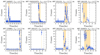 |
Fig. A.1. FXT 0.5–7.0 keV light curves in units of counts in 1 ks bins. The T90 duration for each source is denoted by the orange region, and listed above. The gray dashed line represents the end of the Chandra observation. |
Furthermore, Fig. A.2 confirms that the final sample of FXT candidates is real celestial sources in the sky rather than detector artifacts. Due to Chandra’s Lissajous dither pattern, executed during observation, the X-ray photons of the FXTs are distributed over dozens to hundreds of individual pixels on the detector. The first column of the figure shows the light curves, color-coded by the phase in the light curve evolution. The second column shows the spatial location in x and y chip detector coordinates, also color-coded by time, tracing out a sinusoidal-like evolution in x and y coordinates over time. The third and fourth columns show the x and y position changes (in blue and purple, respectively, over time, with the light curve superimposed in dark gray.
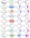 |
Fig. A.2. Lissajous dither pattern in detector coordinates. First column: FXT 0.5–7.0 keV light curves in count units, color-coded as a function of time. Second column:Chandra 0.5–7.0 keV images in detector coordinates, with the same color-coding as a function of time, demonstrating the temporal movement of the source on the detector in response to the Lissajous dither pattern. A flaring pixel would appear as a point on these plots. Third and fourth columns: x (blue) and y (purple) detector coordinates, respectively, of the detected X-ray photons from the FXTs as a function of time, with the candidate light curves superimposed as solid dark gray lines. |
Visibility of the FXTs by the Fermi-GBM instruments.
Appendix B: Forced photometry upper limits
From the flux density measurements of ZTF and ATLAS, we derive upper limits closer to the X-ray trigger time for FXTs 17, 18, 19, 20, 21, and 22. We compute the upper limits AB magnitude by taking 3 times the uncertainty from the forced photometry flux density. The AB magnitude upper limits inferred from the closest observation in time to the transient are given in Table B.1 for the available FXTs and filters.
Simultaneous counterpart 3σ upper limits (AB mag) inferred from forced photometry.
Appendix C: Host-galaxy SED fitting
To derive the host galaxy parameters, we used the existing photometry and the spectral energy distribution (SED) models from the BAGPIPES package (Bayesian Analysis of Galaxies for Physical Inference and Parameter EStimation; Carnall et al. 2018). It fits broadband photometry and spectra with stellar-population models taking star-formation history and the transmission function of neutral and ionized ISM into account via a MultiNest sampling algorithm (Feroz & Hobson 2008; Feroz et al. 2009). BAGPIPES provides posterior distributions for the host-galaxy redshift (z), age, extinction by dust (AV), star-formation rate (SFR), metallicity (Z), stellar mass (M*), and specific star formation rate. To fit the SEDs, we consider a star-formation history (SFH) described by an exponentially decreasing function with a timescale parameter τ (which is probably the most commonly applied SFH model; Simha et al. 2014; Carnall et al. 2019). The models implemented within BAGPIPES are constructed using an Kroupa & Boily (2002) initial mass function (IMF). To model the dust attenuation in the SEDs, we used the theoretical framework developed by Calzetti et al. (2000), where AV is a free parameter within the range of 0.0 to 3.0 mag. For the fitting process, we assumed an exponentially declining star formation history function parametrized by the star formation timescale (free parameter). Fig. C.1 shows the 16th to 84th percentile range for the posterior spectrum, photometry, and the posterior distributions for five fitted host-galaxy parameters.
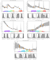 |
Fig. C.1. Best-fitting SED models per FXT. Top panels: Best-fitting SED model obtained from BAGPIPES (Carnall et al. 2018) for each source #1 associated with FXTs 16, 18, 19, 21 and 22, and the relative transmission functions of the different filters used in the fitting process (colored curves). The 16th to 84th percentile range for the posterior spectrum (shaded gray region) and predicted photometry points (orange markers) are shown. The actual photometric data and their uncertainties are given by the blue markers. Bottom panels: Posterior distributions for the five fitted parameters (star-formation rate, age, galaxy stellar mass, metallicity, and redshift) are shown. The 16th, 50th, and 84th percentile posterior values are indicated by the vertical dashed black lines. |
Energetics of the FXT sample.
Below, we describe their most important properties and features one by one:
FXT 16 (CDF-S XT2) is associated with a zspec = 0.738 host galaxy with a relatively flat SED. Fitting its photometry with BAGPIPES at the known redshift, we find that the host galaxy appears to have a low stellar mass and modest star formation rate, consistent with the ones reported in the literature.
For FXT 18, SED fits of the photometric data indicate that the host galaxy has low stellar mass, moderate age, with a low star formation rate and a photometric redshift of ≈0.35.
The field of FXT 19 was observed by HST on 2014-07-10 (three years before the X-ray trigger) in the F606W, F814W, F110W, and F160W filters. The blue host appears to have a low stellar mass, modest star formation rate, and a photometric redshift of zphot = 1.44±0.08. This host galaxy was observed with the WFC3 G102 and G141 grisms from the WFC3 Infrared Spectroscopic Parallel (WISP) Survey, but unfortunately, no significant features are detected in the 2D spectra, aside from strong contamination due to the zero-order spectra of a neighboring star (Atek et al. 2010; Budavári & Lubow 2012; Whitmore et al. 2016).
FXT 20 only has faint g, r and z-band DECam detections, which are too few and too loosely constrained to compute an SED photometric redshift.
For FXT 21, SED fits of the photometric data indicate that the host galaxy is likely massive and relatively old, with a highly uncertain star formation rate and a photometric redshift of 0.85±0.14.
Finally, FXT 22 is located near the extended zspec = 1.5105 galaxy SDSS J134856.75+263946. SED fitting of the photometric data at the known redshift indicates that the host is likely a massive post-starburst galaxy, with a large but highly uncertain star formation rate.
Appendix D: Comparison with Paper I FXTs
This new sample of FXTs discovered in this paper shares timing and host-galaxy property similarities with the previous distant FXTs identified in Quirola-Vásquez et al. (2022) (or Paper I) and other X-ray transients. In that way, Figs. D.1 and D.2 compare the light curves of FXTs identified in this work and in Paper I and the galaxy properties with other transients such as LGRBs, SGRBs, CC-SNe, SNe-Ia, SL-SNe, and FRBs, respectively.
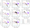 |
Fig. D.1. Light curves of the eight FXTs in 0.3–10 keV luminosity units (converted from 0.5–7 keV light curves assuming best-fit spectral models in Sect. 3.3). Light curves of distant FXTs from Paper I are shown for comparison. We adopt the redshifts listed in Table 9. |
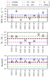 |
Fig. D.2. Comparison of the star-formation rates (top panel), stellar masses (middle panel), and redshifts (bottom panel) of FXT hosts identified in Paper I (FXTs 8, 9 and 14) and this work (FXTs 16, 19, 21 and 22). The mean SFRs, stellar masses, and redshifts from samples of LGRBs (dashed blue line), SGRBs (dashed red line), CC- (dashed cyan line), and Type Ia (dashed orange line) SNe, SL-SNe, and FRBs (dashed black line) are also plotted (Tsvetkov & Bartunov 1993; Prieto et al. 2008; Li et al. 2016; Galbany et al. 2014; Blanchard et al. 2016; Heintz et al. 2020; Schulze et al. 2021; Fong et al. 2022; Qin et al. 2022). |
All Tables
Variability properties of the extragalactic FXT candidates detected and/or discussed in this work obtained by the G–L method, ordered by subsample and date.
Properties of the extragalactic FXT candidates detected and/or discussed in this work, ordered by date.
Best-fit parameters obtained using either a broken power-law (BPL) or a power-law (PL) model fit the X-ray light curves.
Parameters obtained from the literature and by our SED fitting to archival photometric data using the BAGPIPES package (Carnall et al. 2018).
Results of the 0.5–7 keV X-ray spectral fits for the final sample of FXT candidates.
Simultaneous counterpart 3σ upper limits (AB mag) inferred from forced photometry.
All Figures
|
Fig. 1. Histogram (red; left Y-axis) and cumulative (black; right Y-axis) distributions of the exposure time of the 3899 Chandra observations used in this work. The inset provides a zoom-in to show the high-exposure time tail of the distribution. The dashed vertical blue line indicates the median exposure time (=19.7 ks) of the total sample. |
| In the text | |
|
Fig. 2. Comparison of 0.5–7.0 keV net-count distributions for the initial (filled blue histograms) and final (filled black histograms) FXT samples, as well as subsets covered by various purity criteria (color non-filled histograms) for the sample. Net counts are provided by the same regions defined in Sect. 2.4. |
| In the text | |
|
Fig. 3. 0.5–7 keV light curves for each FXT candidate: (1st column) full exposure, in units of counts; (2nd column) zoom in, from the detection of first photon to the end of the exposure, in units of count rate (cts s−1), with log-log scaling and 5 counts per bin. The gray dashed lines show the stop-time per observation regarding the beginning of the transient; (3rd column) long-term light curve, with each point representing individual Chandra exposures (cyan circles with 1-σ error bars) to highlight the significance of detections and nondetections, in units of counts; (4th column) long-term light curve, with each point representing individual Chandra (cyan), XMM-Newton (orange) and Swift-XRT (green) exposures in units of flux (erg s−1 cm−2). For the long-term light curves, the observation including the transient is denoted by a large red star (1-σ error bars), while triangles denote observations with (3-σ) upper limits. All fluxes are reported in the 0.5–7 keV band in the observer’s frame. |
| In the text | |
|
Fig. 4. ATLAS differential photometry of the cyan (c) and orange (o)-bands light curves performed at the position of the FXT candidates. < 5σ data points are shown in hollow circles, while > 5σ data points are shown in solid circles. The blue vertical lines show the epochs when the FXT candidates were detected by Chandra, while the dashed gray lines represent the zero flux. |
| In the text | |
|
Fig. 5. ZTF differential photometry of the g (green points), r (red points) and i-bands (orange points) light curves performed at the position of the FXT candidates. < 5σ data points are shown in hollow circles, while > 5σ data points are shown in solid circles. The blue vertical lines shows the epochs when the FXT candidates were detected by Chandra, while the dashed gray lines represents the zero flux. |
| In the text | |
|
Fig. 6. Archival optical, near-infrared, mid-infrared and X-ray images of extragalactic FXT candidates; the telescope/instrument + filter and FXT ID name are shown in the upper-left corner. Each cutout is centered on the X-ray position, while red circles denote 2σChandra errors in the source localization (1st, 2nd, 3rd and 4th columns) optical band (DECam, Pan-STARRS and HST) images (5th and 6th columns) near-infrared J or H and K (2MASS, UKIRT or VISTA) images; (7th column) 3.4 μm (unWISE) images; and (8th column) X-ray Chandra (ACIS) 0.5–7 keV images. The colored arrows and circles show the localization of the possible host of the FXT candidates. HST images were aligned using the astrometry of Gaia. |
| In the text | |
|
Fig. 7. Sky positions, in Galactic coordinate projection, of FXT candidates: the initial 151 FXT candidates of this work are represented by blue triangles (see Sect. 2.6; some symbols overlap on the sky); the final sample of eight extragalactic FXT candidates from this work are denoted by large red stars (FXTs 20 and 22 overlap on this scale); and the final sample of 14 extragalactic FXTs analyzed in Paper I are shown as orange circles (FXTs 14 and 16 overlap on this scale). The background gray scale encodes the location and number of distinct colocated or closely located observations among the combined 3899 and 5303 Chandra observations used in this work and Paper I, respectively. |
| In the text | |
|
Fig. 8. Light curve and hardness evolution. Top panels: observed 0.5–7.0 keV X-ray light curves in cgs units (blue points), starting at T = 20 s. We also plot the best-fit broken power-law or simple power-law model (red solid lines). The light curves contain five counts per bin. Bottom panels: hardness ratio evolution (the soft and hard energy bands are 0.5–2.0 keV and 2.0–7.0 keV, respectively), following the Bayesian method of Park et al. (2006). The red dashed line denotes a hardness ratio equal to zero. Here, T0 = 0 s is defined as the time when the count rate is 3σ higher than the Poisson background level. |
| In the text | |
|
Fig. 9. X-ray spectra per FXT candidates. Top panels: X-ray spectra (black crosses), in units of counts s−1 keV−1. We also plot the best-fit absorbed power-law (blue lines) spectral model; see Table 7 for the corresponding best-fitting parameters. Bottom panels: residuals (defined as data-model normalized by the uncertainty) of each spectral model. |
| In the text | |
|
Fig. 10. Power-law spectral parameters. Top panel: intrinsic neutral hydrogen column density distribution, evaluated at z = 0 and in units of cm−2, obtained using the power-Law model for extragalactic FXT candidates from this work (orange histogram) and Paper I (blue histogram). The arrows indicate that the z = 0 intrinsic hydrogen column densities are lower bounds. Bottom panel: photon index distribution, obtained using a power-law model, for FXT candidates from this work (orange histogram) and Paper I (blue histogram). Note that the uncertainties on these parameter values for individual sources can be considerable (see Table 7). |
| In the text | |
|
Fig. 11. Hardness ratio comparison. Top panel: hardness ratio of each FXT candidate (using the Bayesian BEHR code; Park et al. 2006) at 1σ confidence level. Bottom panel: hardness-ratio distributions of our final samples of FXTs (orange histogram), compared to the X-ray transients classified as “stars” by Criterion 2 using Gaia (filled cyan histogram) and the sources identified previously as distant FXTs (blue histogram) by Paper I. |
| In the text | |
|
Fig. 12. Color-color diagrams of the potential host galaxies associated with FXTs 16, 18, 19, 20, 21 and 22 (colored stars), “distant” FXTs from Paper I (magenta hexagons), and X-ray sources classified as stars in Paper I (gray filled circles) and here according to Criterion 2 in Sect. 2.7.2 (black filled circles). The expected parameter space of stars with different ages [log(Age) = 7.0 − 10.3], metallicities ([Fe/H] = −3.0 − 0.5), and attenuations (AV = 0.0 − 5.0) taken from the MIST package (Dotter 2016; Choi et al. 2016) are overplotted as cyan regions. |
| In the text | |
|
Fig. 13. Star-forming galaxy main sequence diagram, stellar mass vs. SFR, comparing hosts of FXTs and various other transient classes (one per panel) such as SNe type Ia, Ib, Ic, II (Tsvetkov & Bartunov 1993; Galbany et al. 2014; Schulze et al. 2021), super-luminous SNe (SL-SNe; Schulze et al. 2021), LGRBs (including SN 2020bvc; Chang et al. 2015; Li et al. 2016; Izzo et al. 2020; Ho et al. 2020), low-luminosity LGRBs (LL-LGRBs; GRB 980425, GRB 020903, GRB 030329, GRB 031203, GRB 050826, GRB 060218, and GRB 171205A; Christensen et al. 2008; Michałowski et al. 2014; Levesque 2014; Krühler et al. 2017; Wiersema et al. 2007; Wang et al. 2018; Arabsalmani et al. 2019), SGRBs (including GW 170817 or GRB 170817A; Li et al. 2016; Im et al. 2017; Nugent et al. 2022), TDEs (French et al. 2020), and Paper I FXT candidates (nearby and distant FXTs). Grayscale contours denote the SDSS galaxy distribution from Brinchmann et al. (2004). The solid cyan lines show the best-fit local galaxy main sequence relation from Peng et al. (2010), while the dashed colored lines denote the upward evolution of the boundary separating star-forming and quiescent galaxies as a function of redshift (at z = 0.0, 0.1, 0.2, 0.3, and 0.4; Moustakas et al. 2013). |
| In the text | |
|
Fig. 14. Comparison of the host-galaxy properties of FXTs 16, 19, 21 and 22 (color vertical dashed lines) from Table 6 with the cumulative distributions of galaxy stellar mass (left panel), star-formation rate (center panel), and projected physical offset (right panel) for LGRBs (blue lines; Li et al. 2016; Blanchard et al. 2016), SGRBs (red lines; Fong et al. 2010, 2012, 2014, 2022; Margutti et al. 2012; Sakamoto et al. 2013; Berger et al. 2013b; Nugent et al. 2022), FRBs (black lines; Heintz et al. 2020), CC-SNe and Ia-SNe (cyan and orange lines; Tsvetkov & Bartunov 1993; Prieto et al. 2008; Galbany et al. 2014), and SLSNe (magenta lines; Schulze et al. 2021). |
| In the text | |
|
Fig. 15. Observed cumulative log𝒩–log S and log𝒩–log Fpeak distributions. Left panel: log𝒩–log S distribution of the sample of extragalactic FXTs analyzed in this work (orange line), from Paper I (cyan line), and combined (black line), as a function of fluence (in cgs units). Also shown are two PL models, N(> Fluence)∝S−γ, with slopes γ = 0.52 (red line) and 1.0 (blue dashed line). The γ = 1 line represents the best fit and 1σ error of Arefiev et al. (2003) based on bright FXTs (including Galactic flares). The brightest sources in our sample appear to be consistent with this bright-end extrapolation, although our fainter sources fall up to ∼1 dex below, implying a break. For comparison with Arefiev et al. (2003), we convert all FXT fluences to the 2−10 keV band from their best fits. Right panel: log 𝒩–log Fpeak distribution of the total sample of extragalactic FXTs analyzed in Paper I and this work (black line) and only distant FXTs (orange line). The magenta dashed line shows objects uniformly distributed in Euclidean space ( |
| In the text | |
|
Fig. 16. Peak X-ray luminosity versus redshift and X-ray luminosity function of FXTs. Left panel: peak X-ray luminosity of FXT candidates from Paper I and this work (with known and fiducial redshifts; see Table 9). The green solid and dashed lines indicate peak flux limits of 10−13 (set by our algorithm) and 10−14 erg cm−2 s−1 (approximate Chandra on-axis detector limit), respectively. Right panel: FXT X-ray (0.3–10 keV) luminosity function (XLF) of the total sample from Paper I and this work. The red squares represent the XLF using the seven FXTs with known (photometric or spectroscopic) redshifts, while the blue and green squares show XLFs using all 17 FXTs with known+fiducial redshifts, adopting z = 1.0 and 0.5 for unknown objects, respectively. The solid lines show best-fit power-law models (see Table 10 for values). |
| In the text | |
|
Fig. 17. Volumetric density rate as a function of redshift comparing FXTs (gray filled region, assuming no evolution with redshift and 1-σ confidence; see text for details) and other transients. Left panel: comparison to massive-star related sources such as CC-SNe (dashed orange line; |
| In the text | |
|
Fig. 18. Light curves of the eight FXTs in 0.3–10 keV luminosity units (converted from 0.5–7 keV light curves assuming best-fit spectral models in Sect. 3.3). Several individual transients are overplotted: XRF 080109/SN 2008D (the low-luminosity supernova SBO; solid cyan lines, 27 Mpc); XRF 060218/SN 2006aj (solid blue lines, 145 Mpc); XRF 100316D/SN 2010bh (solid orange lines, 263 Mpc; Barniol Duran et al. 2015; Starling et al. 2011; Modjaz et al. 2009; Evans et al. 2009, 2007; Soderberg et al. 2008; Campana et al. 2006); GRB 110328A or Swift J1644+57 (relativistically beamed TDE; solid black lines, z = 0.3543; Bloom et al. 2011; Levan et al. 2011); J2150−0551 (unbeamed TDE; solid pink line, z = 0.055; Lin et al. 2018). For FXTs 15, 17, 18 and 20 (open symbols), we assume z = 1.0, and for FXTs 16, 19, 21, and 22 we take the redshift values from Table 6. |
| In the text | |
|
Fig. 19. Similar to Fig. 18. The X-ray afterglow light curves of 64 LGRBs plus 32 SGRBs (taken from Bernardini et al. 2012; Lü et al. 2015) are shown as a 2D histogram, while several individual transients are overplotted: GRB 111209A (ultra-long duration LGRB; solid magenta line, z = 0.677; Levan et al. 2014); GRB 170817A (off-axis SGRB, multiplied by ×1000; solid dark green line; Nynka et al. 2018; D’Avanzo et al. 2018; Troja et al. 2020, 2022); SN 2020bvc (the first off-axis LGRB candidate; solid light green line; Izzo et al. 2020), and theoretical off-axis GRB afterglows at different viewing angles θobs (solid and dashed colour lines represents afterglows with isotropic-equivalent energy and circumburst density of 1053 erg, 1 cm−3 and 1051 erg, 0.15 cm−3, respectively; Berger 2014; Ryan et al. 2020; Chrimes et al. 2022). For FXTs 15, 17, 18, and 20 (open symbols), we assume z = 1.0, and for FXTs 16, 19, 21, and 22, we take the redshift values from Table 6. |
| In the text | |
|
Fig. A.1. FXT 0.5–7.0 keV light curves in units of counts in 1 ks bins. The T90 duration for each source is denoted by the orange region, and listed above. The gray dashed line represents the end of the Chandra observation. |
| In the text | |
|
Fig. A.2. Lissajous dither pattern in detector coordinates. First column: FXT 0.5–7.0 keV light curves in count units, color-coded as a function of time. Second column:Chandra 0.5–7.0 keV images in detector coordinates, with the same color-coding as a function of time, demonstrating the temporal movement of the source on the detector in response to the Lissajous dither pattern. A flaring pixel would appear as a point on these plots. Third and fourth columns: x (blue) and y (purple) detector coordinates, respectively, of the detected X-ray photons from the FXTs as a function of time, with the candidate light curves superimposed as solid dark gray lines. |
| In the text | |
|
Fig. C.1. Best-fitting SED models per FXT. Top panels: Best-fitting SED model obtained from BAGPIPES (Carnall et al. 2018) for each source #1 associated with FXTs 16, 18, 19, 21 and 22, and the relative transmission functions of the different filters used in the fitting process (colored curves). The 16th to 84th percentile range for the posterior spectrum (shaded gray region) and predicted photometry points (orange markers) are shown. The actual photometric data and their uncertainties are given by the blue markers. Bottom panels: Posterior distributions for the five fitted parameters (star-formation rate, age, galaxy stellar mass, metallicity, and redshift) are shown. The 16th, 50th, and 84th percentile posterior values are indicated by the vertical dashed black lines. |
| In the text | |
|
Fig. D.1. Light curves of the eight FXTs in 0.3–10 keV luminosity units (converted from 0.5–7 keV light curves assuming best-fit spectral models in Sect. 3.3). Light curves of distant FXTs from Paper I are shown for comparison. We adopt the redshifts listed in Table 9. |
| In the text | |
|
Fig. D.2. Comparison of the star-formation rates (top panel), stellar masses (middle panel), and redshifts (bottom panel) of FXT hosts identified in Paper I (FXTs 8, 9 and 14) and this work (FXTs 16, 19, 21 and 22). The mean SFRs, stellar masses, and redshifts from samples of LGRBs (dashed blue line), SGRBs (dashed red line), CC- (dashed cyan line), and Type Ia (dashed orange line) SNe, SL-SNe, and FRBs (dashed black line) are also plotted (Tsvetkov & Bartunov 1993; Prieto et al. 2008; Li et al. 2016; Galbany et al. 2014; Blanchard et al. 2016; Heintz et al. 2020; Schulze et al. 2021; Fong et al. 2022; Qin et al. 2022). |
| In the text | |
Current usage metrics show cumulative count of Article Views (full-text article views including HTML views, PDF and ePub downloads, according to the available data) and Abstracts Views on Vision4Press platform.
Data correspond to usage on the plateform after 2015. The current usage metrics is available 48-96 hours after online publication and is updated daily on week days.
Initial download of the metrics may take a while.