| Issue |
A&A
Volume 664, August 2022
|
|
|---|---|---|
| Article Number | A60 | |
| Number of page(s) | 36 | |
| Section | Astrophysical processes | |
| DOI | https://doi.org/10.1051/0004-6361/202142802 | |
| Published online | 04 August 2022 | |
Compact molecular gas emission in local LIRGs among low- and high-z galaxies
1
Centro de Astrobiología, (CSIC-INTA), Astrophysics Department, Madrid, Spain
e-mail: This email address is being protected from spambots. You need JavaScript enabled to view it.
2
Telespazio UK, for the European Space Agency (ESA), ESAC, Villanueva de la Cañada, Madrid, Spain
3
Observatorio Astronómico Nacional (OAN-IGN)-Observatorio de Madrid, Alfonso XII, 3, 28014 Madrid, Spain
4
Department of Physics, University of Oxford, Oxford OX1 3RH, UK
5
Cosmic Dawn Center (DAWN), Copenhagen, Denmark
6
Niels Bohr Institute, University of Copenhagen, Jagtvej 128, 2200 Copenhagen, Denmark
7
Centre for Extragalactic Astronomy, Department of Physics, Durham University, South Road, Durham DH1 3LE, UK
8
Institute of Astrophysics, Foundation for Research and Technology – Hellas (FORTH), Heraklion 70013, Greece
9
Instituto de Astrofísica de Andalucía (IAA-CSIC), Apdo. 3004, 18008 Granada, Spain
Received:
1
December
2021
Accepted:
28
March
2022
Abstract
We present new CO(2–1) observations of a representative sample of 24 local (z < 0.02) luminous infrared galaxies (LIRGs) at high spatial resolution (< 100 pc) from the Atacama Large Millimeter/submillimeter Array (ALMA). Our LIRGs lie above the main sequence (MS), with typical stellar masses in the range 1010–1011 M⊙ and SFR ∼ 30 M⊙ yr−1. We derive the effective radii of the CO(2–1) and the 1.3 mm continuum emissions using the curve-of-growth method. LIRGs show an extremely compact cold molecular gas distribution (median RCO ∼ 0.7 kpc), which is a factor 2 smaller than the ionized gas (median RHα ∼ 1.4 kpc), and 3.5 times smaller than the stellar size (median Rstar ∼ 2.4 kpc). The molecular size of LIRGs is similar to that of early-type galaxies (ETGs; RCO ∼ 1 kpc) and about a factor of 6 more compact than local spiral galaxies of similar stellar mass. Only the CO emission in low-z ULIRGs is more compact than these local LIRGs by a factor of 2. Compared to high-z (1 < z < 6) systems, the stellar sizes and masses of local LIRGs are similar to those of high-z MS star-forming galaxies (SFGs) and about a factor of 2–3 lower than submillimeter (submm) galaxies (SMGs). The molecular sizes of high-z MS SFGs and SMGs are larger than those derived for LIRGs by a factor of ∼3 and ∼8, respectively. Contrary to high-z SFGs and SMGs, which have comparable molecular and stellar sizes (median Rstar/RCO = 1.8 and 1.2, respectively), local LIRGs show more centrally concentrated molecular gas distribution (median Rstar/RCO = 3.3). A fraction of the low-z LIRGs and high-z galaxies share a similar range in the size of the ionized gas distribution, from 1 to 4 kpc. However, no LIRGs with a very extended (above 4 kpc) radius are identified, while for high-z galaxies no compact (less than 1 kpc) emission is detected. These results indicate that while low-z LIRGs and high-z MS SFGs have similar stellar masses and sizes, the regions of current star formation (traced by the ionized gas) and of potential star formation (traced by the molecular gas) are substantially smaller in LIRGs, and constrained to the central kiloparsec (kpc) region. High-z galaxies represent a wider population but their star-forming regions are more extended, even covering the entire extent of the galaxy. High-z galaxies have larger fractions of gas than low-z LIRGs, and therefore the formation of stars could be induced by interactions and mergers in extended disks or filaments with sufficiently large molecular gas surface density involving physical mechanisms similar to those identified in the central kpc of LIRGs.
Key words: ISM: molecules / infrared: galaxies / galaxies: ISM / galaxies: starburst / galaxies: evolution
© ESO 2022
1. Introduction
Luminous and ultraluminous infrared galaxies (i.e., LIRGs, LIR = L[8−1000 μm] = 1011 − 1012 L⊙, and ULIRGs, LIR > 1012 L⊙, respectively) host the most extreme star-forming events in the low-z Universe. They are characterized by extreme total IR luminosity, because a large amount of star formation is hidden by dust, which reprocesses the UV photons that originate from hot young stars and/or active galactic nuclei (AGN; U et al. 2012 and references therein) and re-emits them at longer wavelengths, typically in the IR. From the very early investigations, a large fraction of studies tried to determine the mechanism that powers (U)LIRG systems. Both AGN and star forming activity (e.g., Sanders & Mirabel 1996; Rigopoulou et al. 1999; Veilleux 1999; Risaliti et al. 2006; Valiante et al. 2009; Alonso-Herrero et al. 2012) can co-exist in these systems. The fraction of galaxies dominated by the presence of an AGN increases with LIR (Tran et al. 2001; Nardini et al. 2008; Veilleux et al. 2009; Alonso-Herrero et al. 2012), while lower luminosity LIRGs are mainly powered by star formation (see the review by Pérez-Torres et al. 2021). (U)LIRGs show a large variety of morphologies, which suggest different dynamical phases: from isolated disks for low-luminosity LIRGs to a majority of merger remnants for ULIRGs (e.g., Veilleux et al. 2002; Arribas et al. 2004; Kartaltepe et al. 2010). Their dynamical masses typically range between 1010 and 1011 M⊙ (Bellocchi et al. 2013; Crespo Gómez et al. 2021).
These extreme populations are rare in the local Universe (e.g., Lagache et al. 2005), but they are much more numerous at high-z and are supposed to be the dominant contributors to the star formation in the Universe at z > 1 (e.g., Le Floc’h et al. 2005; Pérez-González et al. 2005, 2008; Caputi et al. 2007; Magnelli et al. 2013). Local ULIRGs were initially assumed to be the local counterpart of high-z IR-luminous galaxies discovered by Spitzer and the more luminous submm galaxies (SMGs; e.g. Blain & Phillips 2002; Tacconi et al. 2006). Later on, several studies suggested that high-z (z ∼ 2) ULIRGs and SMGs instead show IR features more similar to those observed in local lower luminosity LIRGs (e.g., Rujopakarn et al. 2011) than to those seen in local ULIRGs. In particular, the far-IR spectral energy distributions (SEDs) of ULIRGs and SMGs at z ∼ 2 differ from those of local galaxies of similar luminosity in that they appear to be as cold as those of lower luminosity galaxies (LIRGs; Muzzin et al. 2010; Wuyts et al. 2011a). Such high-z systems are then assumed to be scaled-up versions in size and star formation efficiency (SFE = SFR/Mstar) of lower luminosity low-z (U)LIRGs, where low-z (U)LIRGs cover a similar SFR range to normal high-z star-forming galaxies (SFGs; < 1000 M⊙ yr−1; Förster Schreiber et al. 2009; Rujopakarn et al. 2011; Wuyts et al. 2011b; Arribas et al. 2012).
At different redshifts, a tight correlation between stellar mass and SFR has been observed in SFGs, which is referred to the main sequence (MS; Elbaz et al. 2007; Wuyts et al. 2011b). Two main categories1 can be identified: galaxies that lie on the MS and those lying above the MS (outliers). This tight correlation has therefore invoked two distinct modes of star formation: the normal star-forming mode that describes galaxies lying on the SFR–Mstar relation (MS galaxies) which evolve through secular processes such as gas accretion (e.g., Dekel et al. 2009; Davé et al. 2010; Genzel et al. 2015), and the starburst mode that describes galaxies falling well above the MS (above-MS galaxies), which are likely driven by major mergers, representing a star-bursting period with respect to the galaxies on the MS (Rodighiero et al. 2011; Wuyts et al. 2011b; Cibinel et al. 2019). Among the outliers, local (U)LIRGs and SMGs at 1 < z < 4 show similar sSFR, possibly boosted by major merger events, although recent studies have found that some SMGs can also be rotating disks (Hodge et al. 2016) supporting the continuum gas accretion scenario through cold gas flow and minor mergers (Dekel et al. 2009).
To shed more light on this scenario, we perform a novel test of the relation between the spatial extents (defined by the half-light radius) of different tracers in a sample of local LIRGs at high spatial resolution (∼90 pc): in particular, the molecular emission traced by 12CO(2–1) (hereafter, CO(2–1)), the 1.3 mm (247 GHz) continuum, and the stellar and ionized gas emissions can be compared. The stellar and ionized gas sizes have been derived in previous works (Arribas et al. 2012; Bellocchi et al. 2013). With the advent of high-resolution instruments such as the Atacama Large Millimeter/Submillimeter Array (ALMA), we are now able to study the molecular emission in local galaxies at spatial resolutions similar to that covered by typical giant molecular clouds (GMCs, ∼100 pc). Low-z LIRGs offer a unique opportunity to study extreme SF events at high linear resolution and signal-to-noise ratio (S/N), and compare them with those observed locally (i.e., spiral galaxies, early-type galaxies (ETGs), and ULIRGs) and at high-z.
Several works have tried to compare the effective size of different components in high-z systems. A large variety of objects covering a wide range in redshifts (1 ≲ z ≲ 6) and galaxy properties have been identified using different criteria (e.g., stellar mass, far-IR luminosity, or optical compactness). These systems can be mainly classified as (i) compact MS SFGs (Barro et al. 2014, 2016), (ii) MS SFGs (Straatman et al. 2015; Tadaki et al. 2017; Förster Schreiber et al. 2018; Puglisi et al. 2019, 2021; Kaasinen et al. 2020; Fujimoto et al. 2020; Wilman et al. 2020; Cheng et al. 2020; Valentino et al. 2020; Hogan et al. 2021), and (iii) extreme SMGs, which mostly lie in the upper envelope of the MS plane (Lang et al. 2019; Chen et al. 2017, 2020; Calistro Rivera et al. 2018; Hodge et al. 2016; Gullberg et al. 2018). According to this classification, some of the so-called MS galaxies mentioned here can also include a few galaxies lying slightly off the MS (e.g., Tadaki et al. 2017; Puglisi et al. 2019; Kaasinen et al. 2020; Valentino et al. 2020): we should consider these systems as lying approximately on the MS at their corresponding redshift.
Characterization of the distribution of all these tracers is key to understanding how the different phases of the interstellar medium (ISM) evolve in size across the cosmic time, studying several types of galaxies, at low- and at high-z. In particular, this enables us to compare the size of the host galaxy (stellar component) with that derived for the ongoing star formation (ionized gas) as well as the size of the regions where stars are forming (molecular gas) in a local sample of LIRGs and compare them with those derived for local spiral galaxies, ETGs, and ULIRGs as well as high-z SFGs and SMGs.
The present paper is structured as follows. In Sects. 2 and 3 we describe the sample and our observations, and the data reduction, respectively. In Sect. 4, we describe our data analysis and the uncertainties related to the methods used. In Sect. 5 we present the results derived for the effective radii of the molecular and continuum components, comparing their values with those obtained for the stellar and ionized emissions. In Sect. 6 we discuss the results and we compare them with those derived for other local and high-z samples. In Sect. 7 we summarize our main findings and present our conclusions. In Appendix A we present the morphological and kinematic classifications used to characterize our systems. Appendix B shows the CO(2–1), continuum at 1.3 mm, and near-IR maps for the whole sample. In Appendix C, the CO(2–1) and Two Micron All Sky Survey (2MASS; Skrutskie et al. 2006) K-band images are compared for the whole sample, ordered according to their increasing molecular size, RCO. Finally in Appendix D, we present the SEDs for the whole sample to estimate the continuum flux loss at 1.3 mm.
Throughout the paper, we consider the cosmology-corrected quantities: H0 = 67.8 km s−1 Mpc−1, ΩM = 0.308, ΩΛ = 0.692. The redshift is corrected to the reference frame defined by the 3K CMB.
2. The sample
2.1. LIR range
The volume-limited sample consists of 21 local LIRGs (24 individual galaxies) at z ≲ 0.02 for which we obtained ALMA data. The sample has been drawn from the IRAS Revised Bright Galaxy Sample (RBGS, Sanders et al. 2003) with distance D ≲ 100 Mpc (a mean distance for the whole sample is D ∼ 75 Mpc, ranging from 41 Mpc to 101 Mpc). Our LIRGs were previously observed in the optical band using VIMOS/VLT by Arribas et al. (2008) and ten of them have also been analyzed in the near-IR using SINFONI/VLT data by Crespo Gómez et al. (2021).
We derived the total IR luminosity from Díaz-Santos et al. (2017), who assumed the luminosity distance, DL, considered in Armus et al. (2009). In particular, for each object, Díaz-Santos et al. (2017) scaled the integrated IRAS IR and far-IR (derived in the wavelength range 42.5–122.5 μm) luminosities with the ratio between the continuum flux density evaluated at 63 μm in the PACS spectrum (measured in the same aperture as the line) and the total IRAS 60 μm flux density. The normalization at 63 μm ensures that the emission can be associated to the dust continuum emission closely related to star formation. Finally, we scaled these values according to the DL used in this work. The derived LIR covers the range of 1010.4 to 1011.7 L⊙ (see Fig. 1) with a uniform distribution, and can therefore be considered representative of the general properties of local LIRGs. For individual galaxies in multiple systems (i.e., ESO 297-G011/-G012 (N/S), IC 4518 E/W and MCG-02-33-098 E/W), the individual contribution to the LIR of the system was derived while taking into account the relative fluxes of the individual galaxies in the MIPS images at 24 μm (see Table 1).
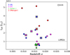 |
Fig. 1. Infrared luminosity versus redshift. The ‘composite’ classification is also shown according to the following color-code: in blue are represented the rotating isolated disk galaxies (0 (R)), in magenta the isolated perturbed disks (0 (P)), in green the interacting systems and in red the post coalescence mergers. Galaxies which belong to the same system (ESO 297-G011/G012, F12596 E/W and IC 4518 E/W) are identified using a solid line. Galaxies containing an AGN are identified by a square. |
General properties of the LIRG sample.
2.2. Activity, morphology, and dynamical phase classification
According to the nuclear optical spectroscopic classification (see Rodríguez-Zaurín et al. 2011), most of the sources are classified as HII galaxies, excluding NGC 7130, which is classified as LINER/Sy2; IC 4518 W and NGC 5135, which are classified as Sy2; and NGC 7469 which is classified as Sy1, along with ESO 297-G011 which shows evidence of an AGN from the optical spectra (Arribas et al. 2014). Following complementary information obtained in the X-rays band, two additional sources (2/24; NGC 2369 and ESO 267-G030) show evidence of an AGN. Mid-IR data are a good tool with which to search for obscured AGN. Alonso-Herrero et al. (2012) searched for highly obscured AGN using mid-IR Spitzer data. Several sources are in common with those studied in this work: except for IC 4518 W, which was previously classified as Sy2, we find that all these systems show a small AGN contribution at 24 μm (i.e., ≲8%), confirming that the AGN contribution does not dominate the galaxy emission in our systems. Thus, we ended up with 7 galaxies in our sample of 24 that show signs of the presence of an AGN (see Table 1).
The sample encompasses a wide variety of morphological types, suggesting different dynamical phases (isolated spiral galaxies, interacting galaxies, and ongoing and post mergers). The majority of our LIRGs are isolated spiral galaxies. In this work, the sources were classified while taking into account both the morphological information from Spitzer/IRAC and Hubble Space Telescope (HST) images and the kinematic information obtained from the ionized (Hα) and molecular (CO) gas phases. In Appendix A, we give a detailed description of this classification (see also Table A.1). Here, we briefly highlight the characteristics of the final “composite” classification used in this work. In particular, we defined four different classes as follows:
-
0 (R): single isolated objects with relatively symmetric disk morphologies, which show the typical kinematic maps of a rotating disk (RD);
-
0 (P): single isolated objects with relatively symmetric disk morphologies but showing a somewhat perturbed kinematics: hereafter perturbed disk (PD);
-
1: objects in a pre-coalescence phase with two well-differentiated nuclei separated by a projected distance of at least 1.5 kpc up to a maximum distance of 15 kpc, showing a perturbed kinematics (hereafter, interacting);
-
2: objects with two nuclei separated by a projected distance ≤1.5 kpc or a single nucleus with a relatively asymmetric morphology, with perturbed or complex kinematics (hereafter, merger).
According to our classification, the majority of our galaxies (two-thirds) show the presence of interaction or past merger activity in their morphology and/or kinematics (i.e., 7/24 are type 0 (P), 4/24 are type 1 and 5/24 are type 2), while the remaining objects (one-third) are disky (0 (R); see Table 1 and Appendix A). In some specific cases, the properties of individual galaxies in multiple systems could be inferred separately and were therefore treated individually.
2.3. SFR – Mstar: location in the MS plane
To estimate the stellar mass Mstar of our sample, we used the integrated K-band near-IR magnitude obtained from 2MASS All-Sky Extended Source Catalog (XSC; Jarrett et al. 2000). The stellar mass estimation in this band is considered a good tracer of the total stellar mass, because the bulk of the luminosity of a SED of simple stellar population (SSP) older than 109 yr is observed in the wavelength range from 0.4 to 2.5 μm. As estimated in previous works (e.g., Alonso-Herrero & Knapen 2001; Alonso-Herrero et al. 2006; Piqueras López et al. 2012; Pereira-Santaella et al. 2015), the visual extinction, AV, in LIRG systems shows typical values of AV < 4 mag, being even smaller in the near-IR bands (e.g., APaα ∼ 0.4 − 1.0 mag). In addition, the AGN contribution in our systems is negligible (see Sect. 2.2), and in the K-band it would only affect the nuclear K-band emission. Furthermore, in the near-IR, the contribution from young stars is found to be often negligible and the scatter in the mass-to-light (M/L) ratio for local LIRGs is relatively small (∼0.4 dex; Pereira-Santaella et al. 2011). We then converted the magnitude to luminosity in the K band, LK, and assuming a (mean) Mstar/LK ratio of 0.4 as derived in Zibetti et al. (2009), we derived the stellar mass in the K band, Mstar2.
We derived the star-formation rate (SFR) from the LIR (see Table 1). This parameter can be considered a good tracer of star formation for all our systems because the AGN contribution in our sample to the total LIR is small (∼5% on average; see also Alonso-Herrero et al. 2012). The LIR contribution is the result of the reprocessed emission originating in star formation regions hidden by the large amount of dust. LIR was converted to SFR following the Kennicutt & Evans (2012) relation with a Kroupa (Kroupa 2001) IMF (see Murphy et al. 2011).
In Fig. 2 (left panel), the results obtained for the SFR versus stellar mass Mstar are shown for our sample. The MS relation defined by Elbaz et al. (2007) for SDSS galaxies at z ∼ 0 is shown with its uncertainties:
![Mathematical equation: $$ \begin{aligned} SFR_{\rm Salp} [M_\odot \mathrm{yr}^{-1}] = 8.7^{+7.4}_{-3.7} \times \frac{M_{\rm star} [M_\odot ]}{10^{11}}^{0.77}. \end{aligned} $$](/articles/aa/full_html/2022/08/aa42802-21/aa42802-21-eq1.gif) (1)
(1)
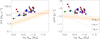 |
Fig. 2. LIRG sample in the SFR - Mstar and sSFR - Mstar planes. Left: SFR as a function of the stellar mass Mstar. The solid and dashed (orange) lines indicate the location of the local MS relation and the 1σ scatter, respectively, obtained by Elbaz et al. (2007) using SDSS galaxies at z ∼ 0 and converted to Kroupa IMF, in agreement with that derived by Whitaker et al. (2012). Our LIRGs are shown according to the color code defined in Fig. 1: isolated disks (RD), (PD), interacting, and merging systems are shown in blue, magenta, green, and red, respectively. The solid lines between the points (green and black) link galaxies that belong to the same system. Galaxies containing an AGN are identified with an empty black square. The horizontal red dashed line represents the threshold SFR to reach the LIRG IR luminosity (log LIR/L⊙ ≥ 11). Right: specific SFR as a function of the stellar mass Mstar. The three (solid, dotted, and dashed) gray lines identify the different SFR regimes (i.e., 1, 5, and 20 M⊙ yr−1, respectively). The MS relation is also shown (in orange). |
This relation used the Salpeter IMF, which was converted to Kroupa according to the formula: SFRKroupa ∼ 0.7 × SFRSalpeter (see Elbaz et al. 2007; Madau & Dickinson 2014). We derived the same MS relation when using the power law defined by Whitaker et al. (2012) at z ∼ 0 using a Chabrier IMF. Our LIRGs lie a factor of 8 above the MS defined by Elbaz et al. (2007), and no clear trend is found among the different morphological classes in the MS plane (Table 2).
Mean (and median) stellar mass Mstar, SFR, and sSFR for the different LIRG subsamples.
Our LIRGs cover the stellar mass range between 1010.0 and 1011.1 M⊙, where most of them (19/24) are in the range 1010.5 and 1011 M⊙. All but one of the mergers (namely F17138-1017) lie in a smaller stellar mass range log Mstar between 10.8 and 11.0 M⊙. The isolated galaxies (type 0) cover a larger range of values, from log Mstar ≲ 10.2 to 11.1 M⊙. The interacting (type 1) systems show quite low stellar masses and SFRs as a result of the disentanglement of the Mstar and SFR contributions of the individual galaxies. Although we only have a small number of AGN objects, our results suggest that LIRGs without an AGN show lower stellar mass (∼40%) than those obtained for LIRGs with an AGN, although with similar SFR. If we distinguish among the different types of galaxies, we see that isolated disks (type 0) and mergers (type 2) share similar stellar masses but mergers are characterized by twice the SFR typical of isolated disks.
We then computed the specific SFR (sSFR = SFR/Mstar) for our sample (right panel Fig. 2), finding two extreme cases for which sSFR > 1 Gyr−1 with low stellar masses (log Mstar ∼ 10.2; ESO 557-G002 and F17138-1017). According to the mean (and median) values, we find that LIRGs with an AGN show sSFR a factor of 2 lower than that derived when LIRGs without an AGN are considered, as a result of their larger (a factor of 2) Mstar. Similar values are obtained for the type 0 and 1 galaxies while type 2 objects show the highest sSFR, although with larger scatter. The typical stellar masses and SFRs derived for our sample seem to be consistent with the starburst scenario (i.e., strong burst of recent, that is < 100 Myr-old, star formation). The most extreme starbursts are those classified as mergers, followed by less extreme isolated disks.
3. Observations and data reduction
3.1. ALMA data
We obtained the CO(2–1) line and the continuum at 247 GHz (∼1.3 mm) emission of a sample of 18 individual local LIRGs observed with ALMA between August 2014 and August 2018, using Band 6 from the project 2017.1.00255.S (PI: Miguel Pereira Santaella). This project was completed with 6 more galaxies that belong to four different projects (see Table 3). The data for two of the LIRGs, IC4687 and ESO320-G030, were previously presented in Pereira-Santaella et al. (2016a,b), and Pereira-Santaella et al. (2020).
Beam sizes of the CO(2–1) and 1.3 mm continuum images for the whole sample.
The total integration time per source was ∼20–30 min in standard mode. The synthesized beam full width at half maximum (FWHM) of the sample ranges between ∼0.2″ and 0.4″: this corresponds to a median size of 85 ± 183 pc at the distance of our LIRGs (see Fig. 3). A combination of the extended and compact configurations was used to achieve the 0.2″ angular resolution and a maximum recoverable scale of 10″–12″ (3–5 kpc). The field of view (FoV) imaged by a single pointing has a diameter ranging between ∼5 and 8 kpc, and the FoV is of ∼10–17 kpc for the three mosaics (NGC 3256, NGC 7469, and MCG-02-33-098). Further details of the observations are listed in Table 3 for each source. Two spectral windows of 1.875 GHz (1.9 MHz ∼ 2.6 km s−1 channel) were centered at the sky frequency 12CO(2–1) transition and 247 GHz continuum spectral window.
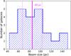 |
Fig. 3. Histogram showing the distribution in physical scales (parsecs) of the size of the beam for the galaxies of the sample. The median and MAD values (solid and dashed magenta lines, respectively) correspond to 85 ± 18 pc. |
The data were calibrated using the standard ALMA reduction software Common Astronomy Software Applications (CASA4 v5.1 McMullin et al. 2007). In the CO(2–1) spectral window, the continuum emission was estimated using the line free channels and then this contribution was subtracted in the uv-plane. For the cleaning of CO(2–1) and continuum data, we used the natural weighting of the uv-plane, obtaining a spatial resolution in the range 50–150 pc (see Fig. 3 and Table 3). The final CO(2–1) data cubes have channels of 4–23.4 MHz (∼5–30 km s−1) and they were corrected for the primary beam. The pixel size is in the range 0.025″–0.06″. For the CO(2–1) data cubes, the 1σ sensitivity is ∼0.4–1.2 mJy beam−1 per 10 km s−1 channel while for the continuum this sensitivity is ∼0.02–0.1 mJy beam−1 (see Table 3).
3.2. Ancillary data
In order to compare the molecular size derived using ALMA data with the ionized and stellar emission in our LIRGs, we considered the results obtained by Arribas et al. (2012) and Bellocchi et al. (2013). Arribas et al. (2012) derived the Hα size of a local sample of (U)LIRGs, which includes all but two5 of the LIRGs of our sample. The analysis was based on integral field spectroscopic VIMOS/VLT data, which cover a FoV of ∼30″ × 30″ at the angular resolution of ∼1.3″. The typical Reff derived for the ionized gas phase are shown in Table 2 in their work. The sizes obtained are intrinsic (i.e., deconvolved) sizes, that is, obtained by subtracting the contribution of the PSF in quadrature. Arribas et al. (2012) computed the effective radii using the curve-of-growth (CoG) and “A/2” methods (see Sect. 4.2.1 for further details). For extended objects, the limited VIMOS FoV only allowed a lower limit to the Reff estimation to be derived.
The bulk of the galaxy stellar component is well traced to first order by the rest-frame near-IR continuum light. For the derivation of the effective radius of the stellar component, we considered the 2MASS data in the K-band from Bellocchi et al. (2013). 2MASS images do not have any limitation by the FoV although they are characterized by a low angular resolution (∼2″). In their work, the Reff were derived using GALFIT and the A/2 methods (see Table B.1 in their work): these methods are discussed in more detail in Sect. 4.2.1.
Furthermore, we considered archival near-IR HST Paα images6 to study how the extinction affects the derivation of the effective radius of the ionized component. Paα images were obtained using the NICMOS2 camera on board the HST in combination with the narrow-band F187N and F190N filters: the FoV of these images is ∼19.5″ × 19.5″ with an angular resolution of FWHM ∼ 0.15″. Most of these observations were previously published by Alonso-Herrero & Knapen (2001), and Alonso-Herrero et al. (2002, 2006).
4. Data analysis
4.1. Molecular gas and 1.3 mm continuum distributions
We generated CO(2–1) and 1.3 mm continuum maps for the whole sample, selecting the emission above 5σ for both maps. These are all shown in Appendix B. The galaxies of our sample show several morphologies: regular (ESO 320-G030, IC 5179), elongated (NGC 2369, IC 4518 E), and irregular objects (MCG 02-33-098 E-W, NGC 3256). Some of them are more compact (F06592-6313, IC 4734) while others more extended (IC 4687, IC 5179, NGC 3110). The 1.3 mm continuum emission is generally quite compact, and in some cases clumpier than CO(2–1). This result is discussed below.
4.2. Effective radius determination and systematic effects
4.2.1. Selection of the methodology
The half-light (or effective) radius (Reff) is defined as the radius which encloses half the total flux emission of the galaxy; it measures the light concentration and depends on the shape of the light profile (Trujillo et al. 2020) as well as on the wavelength considered (e.g., Graham & Worley 2008; Kennedy et al. 2015) and depth of the data.
To derive the size of a system, different methodologies can be applied: GALFIT, the curve-of-growth (CoG) and the so-called “A/2” methods can be used according to the objects considered. GALFIT is based on fitting the observed flux distribution to a galaxy model assuming standard surface brightness profiles (Peng et al. 2002, 2010). This method is accurate as long as the model is a good representation of the actual galaxy flux distribution. However, if the galaxies show irregular or clumpy emission (as in the case of interacting or merger systems) the half-light radii can be obtained from the CoG of the flux at increasingly large apertures. The A/2 method computes the effective (circular) radius as  , where A/2 is the angular extent of the minimum number of pixels (or spaxels) encompassing 50% of the light of the whole galaxy, A. This method is quite often used for high-z systems (e.g., Erb et al. 2004). The A/2 method does not require any knowledge of the galaxy center: indeed, it is not sensitive to the distribution of large and bright regions found within a galaxy but is sensitive to the size of such bright regions. That is, this method depends on the number of pixels required to make up half of the galaxy light, but not on how those pixels are distributed within the FoV. The Reff derived using these methods should be considered within the limitations imposed by the angular resolution, kind of tracer, sensitivity (e.g., Lange et al. 2015), and FoV.
In our specific case, we consider the CoG method (i.e., the flux emission contained in circular apertures of increasing size are derived to compute the radius within which half of the total emission is contained) as a robust way to derive the Reff ; it is commonly applied both at low- and high-z. We considered an equivalent circular aperture as a good approximation of the (major) elliptical aperture. The effective radius in the case of an elliptical aperture is defined as  , where a and b are the major and minor axes, respectively. To check this point, we considered ESO 320-G030, which in CO(2–1) shows a relatively regular shape and surface brightness distribution, and NGC 7130, which shows a more peculiar CO distribution. In the first case, the difference between the effective radius derived using a circular or elliptical aperture agrees within 5% while in the latter the difference agrees within 12%.
We select the center of the (circular) aperture, choosing the peak emission observed in the near-IR using HST/NICMOS F160W (λc = 1.60 μm, FWHM = 0.34 μm) images. When this filter is not available, other near-IR HST filters such as F110W and F190N are considered. When the HST images are not available, the peak emission in the continuum map at 1.3 mm is used. The HST/NICMOS astrometry was corrected using stars within the NICMOS FoV in the F110W or F160W filters and the second Gaia data release (DR2) catalog as reference systems (further details in Sánchez-García et al. 2022).
In our sample, we find very good agreement among the CO(2–1), dust-continuum, and stellar peak emissions. In general, the dynamic center as traced by the stellar emission also nicely overlaps with the dust-continuum emission peak, even in very disturbed objects, such as NGC 3256 and NGC 7130. When no HST images are available, the dust-continuum peak position can be considered a good assumption of the center of the aperture. Furthermore, the CO kinematic center generally agrees well with the stellar peak emission position, although in more complex systems (NGC 3256 and NGC 7130) it is very hard to define. If in disturbed galaxies, like NGC 7130, we modify the center of the aperture to the CO flux emission peak (∼10 pixels), the new RCO and Rcont would be ∼0.72 kpc and 0.185 kpc, respectively, instead of ∼0.7 kpc and ∼0.16 kpc. Then, in such an extreme case, the variation of the effective radius would be of ≲4% and ≲15% for the CO and continuum distributions, respectively. The Reff estimation in the continuum seems to be more affected than in CO(2–1) when changing the center of the aperture as a result of its compact distribution.
The CO(2–1) and 1.3 mm continuum sizes presented in this work are observed; that is, they are not corrected for the beam. The intrinsic CO and 1.3 mm continuum sizes are also resolved (larger than the beam) and are (on average) smaller than the observed size by ≲1% and ≲4%, respectively. Only for one object, ESO 557-G002, would the intrinsic 1.3 mm continuum size be ∼13% smaller than the observed size (64 pc vs. 55 pc) while its intrinsic CO size would be only marginally affected (< 1% smaller).
4.2.2. Correction factors and systemic effects associated to the choice of a method
In order to compare the CO(2–1) and 1.3 mm continuum sizes obtained using the CoG method with those obtained in Arribas et al. (2012) and Bellocchi et al. (2013) for the ionized and stellar components, respectively, we need to correct the effective radii of the stellar component derived using the A/2 method. These radii can indeed be converted to CoG measurements using the relation shown in Fig. 4. In particular, this relation was derived considering the results shown in Arribas et al. (2012) using the CoG and A/2 methods applied to the Hα emission for a local sample of 46 (U)LIRGs. To derive a robust trend able to relate the two methods, we excluded (15) lower limits (due to the limited VIMOS FoV) as well as the results obtained for systems in close7 interaction phase, for which a reliable estimation of their size was not possible. For the remaining 27 galaxies, good agreement is found then between the results from the CoG and A/2 methods and Hα measurements for a given set of data. For this subsample, we found that 0.8 ≲ Reff(CoG)/Reff(A/2) ≲ 2.2, with a median ratio of 1.1. If we include the lower limits, we derive a similar median correction factor (M = 1.16) with larger dispersion.
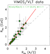 |
Fig. 4. Relation between the CoG and A/2 results derived using VIMOS/VLT (Hα) data (Arribas et al. 2012). To derive this relation, close interacting pairs and the lower limits were excluded (see text). The dashed black line represents the 1:1 relation between the radii while the red solid line is the best fit. The plot shows the mean (standard deviation) and median (M) values of the RHα (CoG)/RHα (A/2) ratio. |
To check the validity of the results achieved using the Hα tracer, we also derived the Reff using the CoG and A/2 methods on a subsample of nine8 LIRGs using the CO(2–1) maps. Among these sources, we selected isolated, interacting, and mergers systems, deriving a mean (median) ratio CoG/‘A/2’ of ∼1.3 ± 0.2 (1.3), which is similar to that derived for the ionized component.
4.2.3. Extinction impact: optical versus near-IR ionized gas tracers. Inclination effects.
In order to study the extinction effect in our sample, we compared the effective radii derived for the ionized gas component traced by the strongest hydrogen emission lines in the optical (Hα) and near-IR (Paα) for a subsample of 12 sources9 from the ALMA sample for which Paα images are available.
The Hα hydrogen recombination line is a direct probe of the current unobscured star formation activity in a galaxy: in the presence of large amounts of dust, as in (U)LIRG systems, its emission could be strongly attenuated. On the other hand, the near-IR Paα tracer is less affected by dust extinction. The combination of the two datasets can provide hints as to the distribution of the extinction in our sample. The higher angular resolution Paα images reveal the morphology of the high-surface-brightness HII regions in great detail, with typical physical scales of the order of a few tens of parsecs, and we are therefore able to resolve the ongoing star forming regions found in our LIRG systems (see Alonso-Herrero et al. 2009). However, NICMOS/HST images may be insensitive to diffuse Paα emission (e.g., Alonso-Herrero et al. 2006; Calzetti et al. 2007), which, in turn, can suffer much less extinction than that affecting the HII regions (e.g., Rieke et al. 2009). On the other hand, VIMOS Hα imaging has a lower angular resolution (physical scale involved is a few hundreds of parsecs), which implies that the observations are more sensitive to the diffuse emission of lower surface brightness. Although the NICMOS data are characterized by a smaller FoV than VIMOS, the bulk of Paα emission for this subsample falls well within the NICMOS FoV. In Fig. 5 we show the Paα emission observed in IC 5179, which is one of the most (intrinsically) extended objects in our sample, and is fully covered by the HST/NICMOS imaging, showing a number of lower surface brightness star-forming regions in addition to the bright nuclear emission.
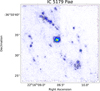 |
Fig. 5. Paα image of the most extended galaxy of the sample, IC 5179, obtained from HST/NIC2 data (filters F187N and F190N). Gray contours highlight the regions in which the star formation is taking place. The FoV is about 19.5″ × 19.5″ with a FWHM ∼ 0.15″. North is up and east to the left. |
In Fig. 6 we compare the effective radius estimations derived using the A/2 and CoG methods for both tracers, without applying the extinction correction to these fluxes. Taking those systems that are sufficiently compact as to be fully covered by the VIMOS FoV, we derived a median ratio RHα/RPα ∼ 1.4. This result should be confirmed with a larger sample covered by a larger (imaging or IFS) FoV. In the bottom panels, the relations between the A/2 and CoG for Hα (left) and Paα (right) are shown. The observed Hα radii derived using the CoG method cover a larger range of values (0.5–3 kpc) than Paα (0.3–1.5 kpc). For this subsample, we found typical mean (median) values of RHα = 1.26 ± 0.71 (1.08) kpc and RPaα = 0.86 ± 0.39 (0.81) kpc. The distribution of the optical tracer is 1.5 (mean value) higher than that derived for the near-IR tracer.
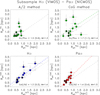 |
Fig. 6. Relation between the observed (not corrected for extinction) Hα and Paα tracers when using A/2 and CoG methods applied to a subsample of 12 galaxies. Lower limits on Hα measurements are due to the limited FoV of VIMOS. Top panels: |


Alonso-Herrero et al. (2009) compared the morphology of the high-surface-brightness HII regions in the Hα and NICMOS Paα emissions for a sample of LIRGs at z < 0.02. Their systems share similar morphology of the high-surface-brightness HII regions in Hα and Paα emission, suggesting that the extinction effects on Hα are not severe, except in the very nuclear regions. Due to the central obscuration, the outer regions have a relatively large fraction of flux in the Hα maps, leading to larger Reff. This would result in a higher estimation of Reff with respect to that derived if the emission were corrected for extinction. Arribas et al. (2012) corrected their images with a simple model extinction in order to understand how the extinction affects the determination of Reff. These authors found that the corrected maps show a mean reduction in size of 25%–30% with respect to the uncorrected values. If we correct our Hα radii for this factor, we end up with an intrinsic mean (median)  (0.8) kpc, which is closer to the value obtained with the Paα tracer.
Furthermore, inclination effects could play an important role when deriving the size of a galaxy. In particular, Graham & Worley (2008) found that the effects of the inclination on the derivation of the Reff between the optical and near-IR bands is very low. Indeed, they found that the intrinsic scale length of a galaxy in the B- and K-bands would be, respectively, 1.35 and 1.05 times lower than the observed scale length (i.e., hobs/hintr ∼ 1.35 and ∼1.05, assuming a mean inclination of 52° as derived for our LIRGs; see Bellocchi et al. 2013; Law et al. 2009). A smaller factor (∼1.2) is derived in the R band. This means that the intrinsic Reff is expected to be slightly lower than the observed radius in the optical and near-IR bands. Under this assumption, we also expect a small conversion at longer (mm) wavelengths: for this reason, no inclination correction has been applied to our sample.
4.3. Instrumental bias: limitation in the FoV, angular resolution, and sensitivity
We now focus our attention on the limitations due to the instrumental setup such as the angular resolution of the observations, their sensitivity, and a limited FoV. We investigate these effects in three galaxies (NGC 1614, NGC 7130, and NGC 3256) classified as post-coalescence systems, which show a relatively complex structure (e.g., tidal tails). These galaxies are good targets to understand how the flux distribution at different bands and angular resolutions affects the Reff estimation in extreme systems. We took into account near-IR continuum images from HST/NIC2 (or HST/WFPC3), 2MASS, and Spitzer/IRAC1 images at 1.6, 2.2, and 3.6 μm, with angular resolutions of ∼0.15″(0.26″), 2″, and 2.4″, respectively. The comparison among the different instrumental setups with that characterizing 2MASS observations allows us to derive the following results. Under the same angular resolution, sensitivity (Benjamin et al. 2003), and FoV (without limitation) as those achieved by Spitzer/IRAC1 data, we derive similar (or ∼30% smaller) Reff between these data sets: RIRAC1 ∼ (30%) × R2MASS . At higher angular resolution (×10) and sensitivity than 2MASS data, as in the case of HST/WFPC3 data characterized by a large FoV (∼2′×2′), we derive similar Reff: RHST/WFPC3 ∼ R2MASS. When the highest angular resolution among the instruments is considered (0.15″) along with very good sensitivity (i.e., slightly lower than WFPC3), but a smaller FoV is involved, as in the case of HST/NIC2, we derive lower Reff for this data set: RNIC2 ≲ 20%×R2MASS .
Thus, under similar conditions (Spitzer/IRAC1 and 2MASS data), slightly smaller (or similar) sizes are derived at 3.6 μm than at smaller wavelength (∼2 μm, i.e., 2MASS H and K bands). High-angular-resolution and high-sensitivity data, such as those achieved by the HST/WFPC3 images, allow us to derive similar sizes to those obtained using 2MASS data in the same band, unless a limited FoV is involved (i.e., HST/NIC2) which then implies smaller effective radii.
5. Results
In this section, we present the Reff results obtained for the CO(2–1) and 1.3 mm emissions using the CoG method of our sample. We compare these results with those previously obtained using the same method for the stellar and ionized (observed Hα) gas emissions. Further comparison between the molecular CO(2–1) and ionized (unobscured) Paα emissions is also discussed.
In Appendix C, we present the CO emission (above 5σ) and K-band maps for the whole sample, ordered according to their increasing molecular effective radii, RCO. The same FoV (14 × 14 kpc2) is considered for all the galaxies for a direct comparison of their size. Reff are given for both the CO(2–1) and K-band maps.
5.1. Molecular and 1.3 mm continuum emissions
The molecular gas distribution derived for our LIRG sample is very compact. It is characterized by RCO sizes spanning a range of values in between a few hundreds of parsecs up to ∼1.3 kpc size (see Table 4). On the other hand, the 1.3 mm continuum emission is even more compact than the molecular gas. We find that the CO(2–1) emission is about twice the size of the 1.3 mm continuum emission, with typical mean (median) sizes of RCO = 0.66 ± 0.33 (0.7) kpc and Rcont = 0.37 ± 0.31 (0.31) kpc. Such compactness could be explained as being due to a sensitivity effect rather than to a limited FoV. In particular, the high angular resolution of our ALMA data prevents us from detecting the contribution of the faintest and most extended emission. As a result, the brightest dust emission then might appear more compact. However, the maximum recoverable scale of these observations is 3–5 kpc, meaning that the extended diffuse and faint emission is unlikely filtered-out. A more detailed analysis of the molecular continuum emission is needed to confirm this point, and will be presented in a future work. To investigate this point further, in Appendix D we present the SED fitting results to quantify the flux loss at 1.3 mm with our ALMA observations. The 1.3 mm continuum fluxes derived with ALMA at > 5σ are well below the SED emission (Flux(SED)/Flux(ALMA) ∼ 2–15) as a result of the sensitivity effects, for which the faint emission at larger radii is not observed. With that in mind, we assume that the effective radii estimation of the 1.3 mm continuum emission is affected by the flux loss of the outer regions at this frequency: for this reason, we do not discuss the results derived for this tracer.
Molecular and 1.3 mm continuum effective radii determinations of the LIRG sample.
On the other hand, we can compare the CO(2–1) fluxes derived with ALMA with those obtained using single dish observations only for a couple of galaxies (IC 4687 and ESO 320-G030; see Pereira-Santaella et al. 2016a,b). For these systems, good agreement is found between the integrated ALMA fluxes and single dish observations, within a factor of < 15%.
5.2. No relation between the molecular size and the morphological type
Our sample shows a large variety of morphology, characterized by compact (Reff < 0.4 kpc), elongated, and complex10 CO(2–1) distributions. The distribution of the sample according to the size of the CO emission (Fig. 7 left) suggests a bimodal behavior, with compact (Reff < 0.4 kpc) and more extended galaxies (Reff > 0.6 kpc). Smaller (median) radii are found for interacting systems (type 1), while mergers (type 2) share similar size with isolated (type 0) objects.
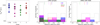 |
Fig. 7. Left: CO(2–1) effective radius as a function of class. Type 0 (R), 0 (P), 1, and 2 are shown in blue, magenta, green, and red, respectively. The median RCO values (horizontal lines) are shown for each class. Empty squares identify galaxies containing an AGN. Middle:RCO distribution for the whole sample (gray solid line) and for the individual subgroups (same color code as in the left panel). The colored vertical lines in the upper part of the panel represent the median values of each distribution, following the same color code. Right:RCO distribution for the whole sample (gray solid line) and for LIRGs with an AGN. |
We derived the following results (see Fig. 7, right): (a) some disks (type 0; 6/14, 43%) have effective radii in the range 0.2 to 0.4 kpc, and between ∼0.6 and 0.8 kpc (5/14, 36%), while 3 of the 14 sources (21%) show radii ∼1.2 kpc; (b) the sizes of the interacting systems peak around 0.3 kpc; (c) finally, mergers are more commonly distributed around 0.7 kpc, with some outliers found at 0.3 and 1.2 kpc. We can therefore claim that no relation has been found between the molecular size, RCO, and the galaxy types.
5.3. The impact of AGN on the molecular gas
As described in Sect. 2, a small number of objects in our sample are classified as Seyfert galaxies or show signs of the presence of an AGN, the contribution of which does not dominate the galaxy emission. When an AGN is present, both the continuum from the active nucleus and young stars can contribute to the ionization of the gas. We distinguished our sample in LIRGs with (w AGN, 7/24) and without an AGN (w/o AGN, 17/24) to look for correlation between them. An extra flux produced by a bright AGN in the nuclear regions of a galaxy is expected to lead to a smaller effective radius estimation (as for the ionized gas emission; see Arribas et al. 2012).
In our particular case, larger (median) molecular radii by a factor of 2 are derived when considering galaxies with an AGN: the majority of the sources without an AGN show RCO sizes within 0.2–0.4 kpc, while LIRGs with an AGN are characterized by larger molecular size (0.4–1.1 kpc; Fig. 7 middle and right panels). A similar trend is observed for the stellar emission, for which we derive larger stellar radii (by a factor of ∼1.3) for those sources containing an AGN. On the other hand, the average RHα of the ionized component is 0.9 times more compact in the presence of an AGN, similar to what was derived by Arribas et al. (2012) (Table 5), without any variation in their median values.
Mean (and median) half-light radius of the different tracers analyzed in the LIRG sample.
Applying the Kolmogorov-Smirnov (KS) test to the estimation of the effective radii derived for the several tracers with or without an AGN, we can see whether the two subsamples are drawn from the same distribution. For the molecular emission, the test suggests that the two subsamples (AGN versus non-AGN) are not drawn from the same parent sample (p-value = 0.08) while for the stellar and ionized (Hα) components we find a better correlation between the two subsamples (p = 0.2 and 0.8, respectively).
The presence of a high surface brightness CO emission located in the extra-nuclear regions (e.g., spiral arms, off-nuclear structures) in LIRGs with an AGN could provide information that could be used to explain the larger molecular size, RCO, derived in these systems.
5.4. A possible relation between RCO and the main sequence parameters?
There is a slight tendency (Fig. 8, left) for the galaxies with higher SFR to have larger CO sizes (Spearman’s rank correlation coefficient ρ = 0.32, with probability of no correlation p = 0.12). This tendency appears to be stronger when the stellar mass is considered (Fig. 8, right), that is, more massive galaxies tend to have large CO sizes (ρ = 0.53, p = 8 × 10⁻³). However, despite the fact that the stellar mass and SFR ranges covered by the LIRG sample span a factor of ten and more (1010 − 1011 M⊙ and 10–100 M⊙ yr−1, respectively), the CO regions are still compact, with sizes of less than 1 kpc.
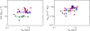 |
Fig. 8. Left: SFR as a function of effective radius RCO. Galaxies containing an AGN are surrounded by a square. A Spearman’s rank correlation coefficient ρ = 0.32 is derived (see text). Right: stellar mass Mstar versus RCO (ρ = 0.53). The different types of galaxies are identified with the same color code as that used in Fig. 7. The orange solid line represents the best fit (linear least square fit). |
5.5. Molecular versus ionized (Paα) emissions
Under the assumption discussed in Sect. 4.2.3, we now compare the Paα results of the ionized component with those derived for the molecular CO(2–1) line (Fig. 9). In this case, we find a tight correlation between the two tracers: indeed, for this subsample (see Sect. 4.2.3) the effective radii derived for CO(2–1) emission are very similar to that derived for the Paα emission. We derived typical mean (median) effective radii of RCO = 0.75 ± 0.33 (0.79) kpc and RPaα = 0.72 ± 0.42 (0.68) kpc. This result highlights the good agreement between the effective radii, indicating that on average the molecular and ionized (Paα) gas distributions are very compact. However, different morphologies can be seen within the sample (Fig. 9). There are systems where the molecular gas is centrally concentrated, while the Paα shows a more extended distribution with star-forming regions in the spiral arms (ESO 320-G030 and IC 4687, probably due to the high extinction of the nuclear regions, AV ∼ 3 mag, for both galaxies; see Alonso-Herrero et al. 2006); some show equally compact nuclear distribution (NGC 1614), while others show similar distributions, both nuclear and extended (IC 5179). As discussed in Pereira-Santaella et al. (2016a,b), a different distribution of the HII regions traced by Paα emission with the molecular CO(2–1) regions within the 100–200 pc scale could suggest that the SF law breaks down on subkpc scales (e.g., Sánchez-García et al. 2022).
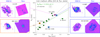 |
Fig. 9. Effective radii derived for the CO(2–1) and Paα tracers using the CoG method. The black dashed line represents the 1:1 relation. The solid green line identifies the derived best fit to the data, which was derived using a linear least squares fit. Two outliers (IC 4687 and ESO 320-G030) are identified for which the RPaα ≳ RCO, while NGC 1614 is characterized by RCO ≳ RPaα. The most extreme RPaα is derived for IC 4518 E, and considered as an upper limit (see text for details). IC 5179 is a galaxy that shows similar effective radii for both gas tracers (RPaα ∼ RCO). |
5.6. Ionized (Hα) and stellar emissions in LIRGs: relations with the molecular distribution
We start by comparing the effective radii derived for the (observed, not corrected for extinction) ionized (Hα) gas and stellar continuum emissions for all galaxies of our sample (Fig. 10 left panel; see Sect. 3.2). We excluded two galaxies (NGC 7469 and IC 4734) from this analysis for which no VIMOS (Hα) data are available. As discussed in Sect. 4.2.1, we considered the results obtained using the CoG method. It is apparent that the stellar emission is characterized by its larger (factor ∼2) size compared to the ionized component. The stellar extension is in the range 1 ≲ Reff ≲ 4 kpc, with a median value of 2.4 kpc, while the typical median Hα size is ∼1.4 kpc. As several Hα measurements are lower limits, the ratio RHα/Rstar = 0.7 can be considered a lower limit as well.
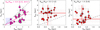 |
Fig. 10. Left: ionized gas size traced by the Hα emission, RHα, as a function of the stellar continuum size in the K band, Rstar. The 1:1 relation is shown using the dashed black line while the best fit is shown in magenta using a solid line; this latter was derived using a linear least square fit. The mean (standard deviation) and median (M) values are shown. Double circles represent galaxies containing an AGN. The dashed blue area represents the size covered by the CO emission for a direct comparison. Middle, right: molecular size versus stellar (middle) and ionized gas (right) distributions. The double circle identifies galaxies with an AGN. The dashed black line represents the 1:1 ratio. The solid lines and the shaded areas represent the median values (MAD). The mode values of these ratios are similar to the median values when considering the stellar results, while we derive a mode of ∼1.3 when considering the Hα results. |
We next compare the stellar and ionized gas distributions to the CO size (Fig. 10 middle and right panels). The ratio between the stellar and the molecular CO sizes gives a (median) value of Rstar/RCO = 3.3 ± 1.0, while the ionized and molecular gas shows more similar values (RHα/RCO = 1.5 ± 0.8). According to the results derived for all the different tracers, we find that in our local LIRGs the stellar emission is the most extended component, for which we derived a typical mean (median) value of 2.2 ± 0.8 (2.4) kpc. The molecular gas is the most compact tracer (if we exclude the 1.3 mm continuum distribution), and is characterized by a typical size of ∼0.7 ± 0.3 (0.7) kpc. According to these results, the molecular gas is a factor 3 more compact than the stellar emission and a factor 2 more compact than the ionized (Hα) gas. As discussed in Sect. 4.2.3, larger Hα sizes than the Paα tracer are derived as a result of the extinction. Indeed, when comparing the molecular distribution with that traced by the ionized Paα emission, the difference decreases, deriving similar effective radii for both tracers.
Furthermore, isolated (type 0) objects seem to show less compact stellar and ionized (Hα) gas distributions (≲2 kpc), while interacting and merger galaxies are more compact (1–1.5 kpc; right panel in Fig. 11). On the other hand, the molecular gas size does not seem to depend on the specific type of galaxy, remaining constant (∼0.7 kpc) among the different subgroups (see Sect. 5.2). Typical mean (and median) values of the different components are summarized in Table 5.
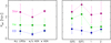 |
Fig. 11. Median effective radii (and MAD) derived for the different tracers and subsamples. The stellar, ionized, and CO(2–1) Reff are shown in magenta, green, and blue, respectively. Left: median values for the whole sample are shown (i.e., ‘ALL LIRGs’), along with the median values derived for the LIRG subsample with (w AGN) and without (w/o AGN) an AGN. Right: median Reff for the four subsamples defined in Table 1 (0(R) 0(P), 1, 2) are shown. |
6. Discussion
6.1. LIRGs versus low-z ETGs, spiral galaxies, and ULIRGs
The molecular and stellar sizes have been studied at low-z for spiral galaxies (Bolatto et al. 201711 and Leroy et al. 202112) and ETGs (i.e., ellipticals and lenticulars; Cappellari et al. 2013a; Davis et al. 2013, 201413). Recently, Pereira-Santaella et al. (2021) analyzed a local sample of ULIRGs using ALMA data, for which they derived the RCO and Rcont sizes. Here, we studied, for the first time, the corresponding molecular and stellar sizes for luminous SFGs located above the MS of local SFGs. Their relation with the SFR and stellar mass parameters is also investigated and compared within the aforementioned local systems.
6.1.1. SFR versusRCO
LIRGs are completely decoupled from spiral galaxies and ETGs in the SFR14–RCO diagram (see Fig. 12 left panel). While spiral galaxies15 are extended systems with a CO(2–1) radius of about 2 to 10 kpc, LIRGs have radii of about a factor ≲6 smaller. Moreover, the sizes of LIRGs cover a range similar to that covered by the sizes of ETGs, while their SFR is a factor 60 higher than for ETGs. The large discrepancy in the molecular size between spiral galaxies and local LIRGs seems to be in agreement with what is discussed in Bolatto et al. (2017): these authors found that galaxies that are more compact in the molecular gas than in stars tend to show signs of interaction (the presence of a bar can also affect the emission distribution). The majority of our galaxies show evidence of interactions or past merger activity, for which type 0 PD and 1 galaxies show the most compact molecular size. On the other hand, merger (type 2) LIRGs show similar molecular sizes to rotating disks: therefore, interactions may play an important role in the compaction of the molecular size, although this requires further investigation. The work by Pereira-Santaella et al. (2021) seems to support the aforementioned result: these authors derived still more compact molecular size for their sources with respect to our LIRGs. Their sources are more extreme in terms of SFR (∼340 M⊙ yr−1) and even show a more disturbed morphology. Their molecular size is a factor 2 more compact than that of our LIRGs (see Table 6).
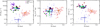 |
Fig. 12. Distribution of LIRGs and other low-z galaxy samples in the SFR–RCO (left), Mstar–RCO (middle), and sSFR–RCO (right) planes. Our LIRGs are shown according to the color code presented in Fig. 1. Local spiral galaxy (gray, red-contoured diamonds) values are taken from the EDGE-CALIFA survey (Bolatto et al. 2017) while ETGs (blue contoured, down-pointing triangles) are taken from the ATLAS3D sample (Cappellari et al. 2013a). ULIRG (purple pentagons) values are derived from ALMA data (Pereira-Santaella et al. 2021). The median value of each sample is shown according to the following color code: purple for ULIRGs, light green for interacting and merger LIRGs, light blue for disky (i.e., RD and PD) LIRGs, orange for spiral galaxies, and dark blue for ETGs. In ULIRGs, the AGN contribution has been removed to estimate their SFRs. |
Mean (and median) half-light radius of the different tracers along with their stellar mass for local and high-z systems.
The derived sSFR of the different samples follows a similar trend to that shown for the SFR parameter. Local spiral galaxies show an sSFR of ∼10−10 yr−1 while ETGs are characterized by a sSFR a factor of 100 lower than that of local spiral galaxies.
6.1.2. Stellar mass versusRCO
In the stellar mass–RCO diagram (Fig. 12 right panel), LIRGs cover a mass range similar to that of low-z samples of spiral galaxies and ETGs, with values in the 1010–1011 M⊙ range. Compared with different types of low-z galaxies, LIRGs are characterized by being located in galaxy hosts with intermediate stellar mass (∼5 × 10¹⁰ M⊙; Table 6), forming stars at rates a factor of ≳10 above spiral galaxies, and with compact CO sizes of RCO ∼ 0.7 kpc, similar to that of ETGs (RCO ∼ 1 kpc).
6.1.3. Stellar mass–size plane
A different trend from that derived for the stellar mass and molecular size components is derived for our sample when the stellar size is considered (Fig. 13). As before, local spiral galaxies (i.e., MS SFGs from Leroy et al. 2021) and ETGs are included in the diagram. LIRGs share similar stellar mass and stellar size with ETGs, while they are more compact (by a factor ∼5) and more massive (by a factor ≲2) than local MS SFGs (see Table 7). From Leroy et al. (2013), we know that the distributions of molecular gas and stellar disk in galaxies follow each other closely in nearby disk galaxies (Rstar ∼ RCO), while the stellar size is larger than the molecular size for ETGs and for our LIRGs by a factor of ≲3.
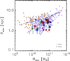 |
Fig. 13. Mass–size distribution for our LIRGs including ETGs and local spiral galaxies (i.e., MS SFGs; Leroy et al. 2021). ETGs are marked with (blue contour) down-pointing triangles and MS SFGs with up-pointing orange triangles. LIRGs are identified following the color code used in previous figures. The blue and red slopes represent the mass–size relations derived by Shen et al. (2003) (see also Fernández Lorenzo et al. 2013) for late- and early-type local galaxies, respectively. |
Ratios of the molecular, ionized and stellar ISM distributions of different types of galaxies relative to those of LIRGs.
According to evolutionary scenarios, many works support the idea that (U)LIRGs can transform gas-rich spiral galaxies into intermediate-(stellar)mass (1010–1011 M⊙) elliptical galaxies through merger events (Genzel et al. 2001; Tacconi et al. 2002; Dasyra et al. 2006b,a; Kawakatu et al. 2006; Cappellari et al. 2013a). The kinematic study of local (U)LIRGs (Bellocchi et al. 2013) highlights that these systems fill the gap between rotation-dominated spiral galaxies and dispersion-dominated ETGs in the v/σ–σ plane. Following our present results, most of the LIRGs share similar properties with ETGs while only a few overlap with the region covered by spiral galaxies.
6.2. LIRGs versus high-z SFGs
Deep cosmological imaging surveys have identified a wide variety of high-z galaxies ranging from quiescent systems (QGs; Straatman et al. 2015) to compact SFGs (cSFGs; Barro et al. 2014, 2016), MS SFGs (Straatman et al. 2015; Tadaki et al. 2017; Förster Schreiber et al. 2018; Puglisi et al. 2019; Cheng et al. 2020; Kaasinen et al. 2020; Valentino et al. 2020 and Puglisi et al. 202116), and more extreme starbursts which generally lie above the MS17, as in the case of SMGs (Hodge et al. 2016; Chen et al. 2017, 2020; Calistro Rivera et al. 2018; Gullberg et al. 2018; Lang et al. 2019; see Table 6).
All these systems were selected using different criteria (i.e., stellar mass, optical radius, or IR luminosity) and observational techniques also covering a broad range of redshifts (1 ≲ z ≲ 6) and galaxy properties. Therefore, they represent the rich diversity of galaxies found during the first half of the history of the Universe. The comparison between the results derived for our LIRGs and a compilation of measurements for different samples of high-z systems will help to better understand how galaxies form and evolve at different cosmic times. In the following, such comparisons in the stellar-mass–size plane (Mstar − Rstar) and in the sizes of the (molecular and ionized) ISM versus their stellar host are presented and discussed.
6.2.1. LIRGs versus high-z SFGs. Stellar hosts
The vast majority of high-z galaxies have masses in the ∼1010 − 2 × 10¹¹ M⊙ mass range, but their sizes cover a much wider range, which reflects the large variety of systems considered at high-z (Fig. 14, Table 6). Indeed, the stellar hosts can be divided in three broad classes according to their effective radii: (i) compact hosts with radii of less than 1 kpc, (ii) star-forming galaxies with intermediate sizes between 1 and 4 kpc, and (iii) extended hosts with radii above 4 kpc and up to 10 kpc. The stellar mass and size of the low-z LIRGs are consistent with those of the intermediate-size SFGs and are well differentiated from those of both the compact and the extended hosts. Among high-z systems, SMG hosts are significantly more massive than local LIRGs by a (median) factor of ∼3 and are also more extended (i.e., stellar size, that is, by up to a factor of ∼2 (Table 7). On the other hand, low-z LIRGs appear a factor about two larger than the massive, H-band-selected, compact SFGs at redshift 2 (Barro et al. 2014).
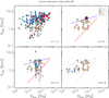 |
Fig. 14. Mass–size distribution for our LIRGs and high-z galaxies (Table 6). LIRGs from this work are shown using light orange circles. High-z SFG and SMG data are taken from the following works: SMGs from Hodge et al. (2016), Chen et al. (2017), Calistro Rivera et al. (2018), and Lang et al. (2019) and SFGs from Barro et al. (2014), Straatman et al. (2015), Tadaki et al. (2017), Förster Schreiber et al. (2018), Cheng et al. (2020), Fujimoto et al. (2020), Kaasinen et al. (2020), Valentino et al. (2020), and Puglisi et al. (2021). The high-z data are shown following the color and symbol code shown in the legend. The blue and red lines in each redshift range represent the mass–size relations for late- and early-type galaxies, respectively, at z ∼ 1.75, 2.25, and 2.75 derived from the 3D-HST+CANDELS surveys (van der Wel et al. 2014). At z = 4 − 6, the mass–size relation for late- and early-type galaxies has not yet been derived, and so the dashed blue and red lines still show the behavior considered at z = 3 − 4. |
The comparison with MS SFGs indicates that low-z LIRGs have stellar sizes and masses similar to those of K-band-selected SFGs at redshifts 3–4 (Straatman et al. 2015). However, LIRGs appear (on average) slightly smaller in size (factor 1.3) than the MS SFGs at redshifts ∼1–2 (Förster Schreiber et al. 2018; Valentino et al. 2020; Puglisi et al. 2021) while their masses (average of 5.6 × 10¹⁰ M⊙) are within the wide range of stellar masses (from 4.3 to 20.0 × 10¹⁰ M⊙) covered by the hosts of the MS SFGs. These results indicate that LIRGs, which represent the bursty above-MS SFGs at low-z, appear to be similar to the bulk population of MS SFGs at intermediate redshifts (z ∼ 1 − 4) in terms of the stellar mass and size of their hosts.
Wang et al. (2018) proposed a two-step scenario to explain how local galaxies evolve from extended star-forming galaxies (eSFGs), through compact star-forming galaxies (cSFGs), to quenched galaxies (QGs). According to this scenario, eSFGs are transformed into cSFGs through compaction mechanisms like minor mergers or interactions with close companions. These mechanisms play a role in enhancing star formation and contributing to the build up of the stellar cores or bulges. At low-z, the compaction processes are more gentle and have longer timescales than those found in the high-z (z ∼ 1) Universe (e.g., Zolotov et al. 2015), which are mainly triggered by major merger events. The quenching mechanism is needed to consume or lose the cold gas in these systems, although they are still able to sustain their star formation activity and the central stellar mass assembly. Finally, from cSFGs to QGs, Wang et al. (2018) proposed that a strong dissipation process takes place, in which the systems consume all their cold gas and quench their SFR as well as the build up of their bulges or stellar cores.
At high-z, a similar scenario has been suggested by Barro et al. (2014), who found that compact SFGs (cSFGs) at z ∼ 2 − 3 could be the natural progenitors of compact QGs (cQGs) at z ∼ 2. In this respect, it is interesting to note that all the low-z LIRGs as well as a large fraction of the high-z galaxies appear in the stellar mass–size diagram (Fig. 14) in between the relations of early- and late-type galaxies at z ∼ 1.75 (typical redshift value for the majority of the high-z systems considered in this work), as derived from the 3D-HST and CANDELS surveys (van der Wel et al. 2014 and references therein). As observed in local LIRGs, distant SMG populations also show a mixture of dynamical phases, hosting merger-driven starbursts (Aguirre et al. 2013) as well as ordered rotating disks (Hodge et al. 2016). This could indicate that many of the high-z galaxies could be in a transitory phase related to tidally perturbed disks or galaxies involved in interactions and mergers, such as low-z LIRGs. Deciphering whether or not this transitory phase represents the evolution from extended disks to compact spheroids requires spatially resolved kinematical information traced by the molecular and ionized ISM.
6.2.2. LIRGs versus high-z SFGs: Sizes of the (un)obscured star formation traced by molecular and ionized ISM
To further explore these evolutionary scenarios empirically, a direct comparison between the tracers of the ISM and the host galaxy is required both at low- and high-z. While the properties of the stellar hosts are traced by the optical and near-IR continuum, the raw molecular material that will be transformed into stars is traced by the CO-emitting gas, while the active regions of obscured and unobscured star formation are traced by the continuum dust emission and hydrogen emission lines, respectively. Thus, the effective radius of the dust and the molecular and ionized gas relative to the stellar light distribution in these galaxies will provide key information about how galaxies build their stellar mass, and how young, massive starbursts could impact the stellar host through stellar winds, and affect its evolution (see Table 6 and Fig. 15). However, simultaneous information for all these tracers is still very limited for high-z samples, in particular when it comes to the ionized component of the ISM traced by the hydrogen lines. This will change in the near future with the advent of spectroscopy in the near- and mid-IR spectral ranges with the James Webb Space Telescope (JWST). As the measurements are very limited for high-z samples, we grouped the various samples into three main categories, independent of their redshift: (i) the compact SFGs, selected as bright H-band-selected galaxies, (iii) the regular SFGs, which are mostly galaxies classified as MS SFGs at their respective redshift range, and (iii) the SMGs, which are extreme starbursts above the MS of SFGs (see Tables 6 and 7 for details).
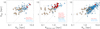 |
Fig. 15. Ratios of different tracers in high-z (z = 2 − 2.5) galaxy samples relative to the low-z LIRG sample (Table 6). Left: stellar versus molecular size. Middle: stellar versus mm/submm (dust-) continuum size. Right: stellar versus ionized gas size. Our sample is shown using light orange circles, while the high-z galaxies are shown following the same symbol and color code shown in Fig. 14. In each panel, we report the references from which the high-z data are taken. Rmm cont derived for our LIRGs were derived from our 1.3 mm ALMA observations, which we considered as lower limits due to the limited sensitivity of our observations. |
LIRGs appear as more compact than high-z SFGs in their molecular gas distribution (factor 2.6 smaller) while having a slightly smaller size (factor 1.3 smaller) in their stellar host (Fig. 15, left). The difference is even larger when comparing with the few SMGs and extended SFGs with available data. SMGs and extended SFGs are far larger (factors ∼8) than LIRGs in their molecular gas while they show only two times larger size than LIRGs in their stellar host. In summary, the distribution of the molecular gas (i.e., the raw material for the formation of new stars) in high-z galaxies is more extended than in low-z LIRGs by factors of between 2.6 and 7.8 in extremely extended galaxies. Moreover, while all LIRGs appear to be located far away from the 1:1 stellar-to-molecular radius relation, high-z SFGs and SMGs tend to be closer, with similar CO and stellar sizes in several systems. Up to now, the number of high-z galaxies with available measurements of the molecular, ionized, and stellar light distributions is quite low, and so the relations found here should be investigated further with larger samples in order to draw firm conclusions.
If the molecular size (CO) traces the regions of future in situ star formation in galaxies, this result could indicate a key difference in the process of star formation and evolution of high-z galaxies with respect to that of starburst galaxies in the nearby Universe: while the star formation in LIRGs is concentrated in their central regions, in high-z systems, the star-formation can proceed over the entire extent of the galaxy. However, to validate this scenario, the size of the active regions of star formation, both obscured and unobscured, relative to the stellar host needs to be established. This comparison can be obtained by measuring the size of the far-IR-continuum-emitting region (Fig. 15, middle) and of the hydrogen recombination lines Hα (Fig. 15, right), which are considered to be tracers of the dust and ionized gas emission associated with dust-enshrouded and unobscured star-formation, respectively.
Several works have studied the dust-continuum emission at 870 μm in high-z SFGs as a proxy for dust-obscured star formation (e.g., Simpson et al. 2015; Lang et al. 2019). This component is found to be compact and centrally concentrated, being a common feature among massive (∼1011 M⊙) high-z SFGs and SMGs (e.g., Simpson et al. 2015; Hodge et al. 2016; Chen et al. 2017; Tadaki et al. 2017; Calistro Rivera et al. 2018; Kaasinen et al. 2020; see Table 6). Unlike local spiral galaxies (e.g. KINGFISH sample; Hunt et al. 2015), for which the dust shares similar scales to the stellar disks (Rdust ∼ Rstar), these high-z SF systems are characterized by centrally enhanced far-IR continuum emission. The compactness of the dust emission with respect to the stellar host in high-z SFGs might be due to the high gas fractions observed in the high-z systems compared to z ∼ 0 objects (Lang et al. 2019). This will involve the presence of very intense and highly obscured star formation with the subsequent growth of stellar mass, mostly in the central regions of these galaxies. However, high-z SFGs and SMGs do not appear to be as compact, in general, as low-z LIRGs (see Fig. 15 where Rcont values at 1.3 mm for the sample of LIRGs are also presented). Even if the sizes measured in LIRGs (average Rcont of 0.37 kpc) could be considered as a lower limit to the real size because of sensitivity effects, the size would not likely be larger than a factor ∼2 if the dust distribution follows the molecular gas emission (average RCO of 0.66 kpc). Moreover, the sizes of the far-IR continuum emission in LIRGs are similar to those derived in a sample of the most luminous LIRGs and ULIRGs using the 33 GHz radio emission Barcos-Muñoz et al. (2017), GOALS survey). This could therefore represent an intrinsically structural distinction between LIRGs and high-z SFGs in that most high-z systems appear to be far more extended than LIRGs in their dust emission relative to the size of their host. However, the number of high-z galaxies with high-angular resolution (≤0.1″–0.2″) ALMA observations is still scarce, and data on larger samples are required before firm conclusions can be drawn.
The size of the ongoing (unobscured) star formation in high-z SFGs as well as in low-z LIRGs is traditionally traced by the Hα emission line in the optical (Fig. 15, right panel; Chen et al. 2017, 2020; Wilman et al. 2020). Detection of other far-IR lines, such as the [CII]158 μm emission line, with high angular resolution has also been carried out in systems in the redshift range of 4 to 6 as part of the ALPINE survey (Fujimoto et al. 2020), for which a typical size of R[CII] ∼ 2.2 kpc was derived. However, [CII] not only traces ionized gas but also the PDR interface between the atomic and molecular gas phases (Lagache et al. 2018; Zanella et al. 2018; Heintz et al. 2021 and references therein).
The sizes of the ionized gas relative to that of far-IR continuum emission in low-z LIRGs and high-z SFGs show some relevant differences. On the one hand, the size of the ionized gas is in general larger than that of the far-IR emission (e.g., Chen et al. 2017, 2020), and is closer to the size of the host galaxy (i.e., closer to the 1:1 relation represented in Fig. 15 right; see Chen et al. 2017, 2020; Wilman et al. 2020). As presented by Popping et al. (2021) in their simulations, the smaller observed-frame 850 μm half-light radius compared to the observed-frame 1.6 μm half-size can be explained as the result of obscuration of the stellar emission at 1.6 μm. Indeed, dust plays an important role in attenuating the 1.6 μm emission in the inner regions of the galaxies (flatter profile), where larger stellar sizes are derived with respect to the case where no dust attenuation is considered. The compactness increases with redshift because the observed H-band emission traces bluer rest-frame wavelengths, which are more affected by the dust attenuation at increasing redshift.
On the other hand, while a fraction of the LIRGs and high-z SFGs share similar sizes (1 to 4 kpc effective radius) in their ionized gas distribution, the two samples are well differentiated in their overall distribution. A substantial fraction of high-z SFGs have very extended Hα-emitting regions with effective radii of up to 10 kpc, and even larger. This is in agreement with the results found by Nelson et al. (2016). These latter authors analyzed a large sample of SFGs observed at z ∼ 1 and found that their ionized Hα emission is more extended than the stellar continuum emission, demonstrating that galaxies at this epoch are growing in size due to star formation. Their result is consistent with inside-out assembly of galactic disks.
On the contrary, half of the low-z LIRGs have sizes of less than 1 kpc; such sizes are not present in high-z SFGs. If the ionized gas represents the size of the ongoing unobscured star formation regions and associated extended nebulae due to outflows and stellar winds, these results indicate that, in general, high-z systems are forming stars in regions distributed over the entire host galaxy while low-z LIRGs are concentrated in smaller central regions. However, the size of the ionized gas is larger than the stellar host in an important fraction of the high-z systems (Wilman et al. 2020; see Fig. 15, right panel). In these systems, the size of the ionized gas may not necessarily trace the real distribution of the star-forming clumps but rather the extended ionized nebulae in the gas-rich environment, as expected in high-z galaxies. Similar to the extended ionized nebulae around quasars, ionizing photons could reach further out and ionize regions well outside the star-forming clumps, even beyond the size of the stellar host.
7. Conclusions
We present the first study that provides detailed measurements of the size (i.e., effective radius) of the molecular gas traced by CO(2–1) in a sample of 21 LIRG systems at low-z. To this aim, we used high-resolution ALMA data, which allow us to reach subkpc spatial resolution scale (< 100 pc, i.e., the size of GMCs). The sample encompasses a wide variety of morphological types, suggesting different dynamical phases (isolated spiral galaxies, interacting galaxies, and ongoing and post-coalescence mergers). All LIRGs are characterized by SFR and stellar masses that place them “above” MS plane at low-z. The sample also represents the closest known analogs to the intermediate- and high-z IR luminous star-forming galaxies.
We performed a comprehensive study of the molecular, stellar (Bellocchi et al. 2013), and ionized (Arribas et al. 2012) gas distributions and their relative sizes. Comparison samples of local galaxies and high-z systems have also been included in order to place the low-z LIRGs in a general context. The main results of the present study can be summarized as follows:
Low-zLIRGs:
-
The molecular gas distribution as traced by the CO(2–1) line is compact in local LIRGs and concentrated in the central regions, with typical (median) RCO ∼ 0.7 kpc. The stellar host and the ionized gas distribution in these systems are factors of ∼3.5 and ∼2 larger than the molecular distribution, respectively. The continuum size at 1.3 mm is half the molecular size, but this should be considered as a lower limit because it is affected by the sensitivity of our observations.
Comparison with low-z spiral galaxies, ETGs, and ULIRGs:
-
LIRGs are indistinguishable from ETGs in the Mstar − Rstar plane, sharing a similar range in stellar mass and size. However, LIRGs have a more compact stellar host than that of local spiral galaxies, by a factor 1.6. This seems to support the evolutionary scenario in which LIRGs can transform spiral galaxies into elliptical galaxies (Genzel et al. 2001; Tacconi et al. 2002; Dasyra et al. 2006b);
-
LIRGs are well separated from low-z spiral galaxies and ETGs in the SFR versus CO size plane as a consequence of their SFR and size: the molecular size of LIRGs is about six times more compact than that of local spiral galaxies of similar stellar masses, while being similar to that of local ETGs, although characterized by higher SFR.
Comparison with high-z SFGs:
-
LIRGs, representing the population of bursty above-MS SFGs at low-z, appear to be similar to the bulk population of MS SFGs at intermediate redshifts (z ∼ 1 − 4) in terms of their stellar mass and the size of their stellar hosts.
-
LIRGs appear to be more compact than high-z SFGs in their molecular gas distribution (factor 2.6 smaller) and appear to have slightly smaller stellar size than high-z SFGs, that is, by a factor of 1.3. Also, while all LIRGs appear to lie a factor of ∼3 above the 1:1 stellar-to-CO radius relation, the high-z SFGs tend to be closer, that is, with similar CO and stellar sizes in several galaxies (i.e., Chen et al. 2017; Calistro Rivera et al. 2018; Kaasinen et al. 2020 and Puglisi et al. 2021).
-
The size of the ionized gas distribution in LIRGs and high-z SFGs is larger than the distribution of far-IR emission, and is closer to the size of the host galaxy (i.e., closer to the 1:1 stellar to ionized gas radius relation). Excluding a small fraction of the LIRGs, that is those that share similar ionized gas distribution (1 to 4 kpc effective radius) with the high-z SFGs analyzed in Wilman et al. (2020), these two populations show different distributions, with high-z systems being found on the 1:1 relation. A substantial fraction of high-z SFGs have very extended Hα-emitting regions with effective radii of up to 10 kpc (Nelson et al. 2016), and even larger, with no LIRGs with sizes above 4 kpc. On the other hand, half of the low-z LIRGs are less than 1 kpc in size, while no high-z SFGs of this size are observed.
At z ∼ 2 red and dead (passive) galaxies already exist at these cosmic epochs and form a separate sequence below the MS of SFGs.
The uncertainties associated to the stellar mass derivation are obtained taking into account the magnitude uncertainties derived in the K band from the 2MASS Extended Source Catalogue (XSC) along with the 0.4 dex uncertainty associated to the M/L ratio.
Throughout the paper, the uncertainty associated to a median value is computed as the median absolute deviation. This uncertainty returns the median absolute deviation of a data set from the median, i.e., median(|data - median(data)|). It is a proxy for the standard deviation, but is more resistant against outliers.
The galaxies NGC 7469 and IC 4734 are not included in their analysis.
We excluded F06035-7102, F06206-6315, F08520-6850, and F23128-5919 (see Bellocchi et al. 2013). The effective radius of the galaxy F12596-1529 was not available (Arribas et al. 2014).
We considered NGC 3110 and NGC 7469 as isolated galaxies, IC 4687 N, IC 4518 E and W, ESO 297-G011, and ESO297-G012 as interacting galaxies, and NGC 1614 and IRAS F17138-1017 as merger systems.
The following galaxies were considered: ESO 320-G030, IC 4687, IC 5179, NGC 7130, NGC 1614, NGC 3256, NGC 3110, NGC 2369, NGC 5135, IRAS F17138-1017, IC 4518 E and W.
Compact systems include IC 4734, ESO 297-G012 and ESO 320-G030 as type 0 (R) galaxies, ESO 319-G022, ESO 557-G002 and F06592-6313 as type 0 (P) and ESO 507-G070 as type 2 objects, elongated systems include ESO 507-G070 and NGC 2369 and complex systems include NGC3256.
In Bolatto et al. (2017) interferometric CO(1–0) observations made with the Combined Array for Millimeter-wave Astronomy (CARMA) interferometer are presented, with galaxies taken from the Extragalactic Database for Galaxy Evolution survey (EDGE) at an angular resolution of ∼4″–5″. A total of 126 galaxies (hereafter, spiral galaxies EDGE-CALIFA) were selected at a distance of < 120 Mpc, deriving the molecular size RCO as the radius enclosing half the CO(1–0) flux.
Leroy et al. (2021) analyzed a representative sample of 90 nearby MS SFGs at a distance of < 90 Mpc observed by the Physics at High Angular resolution in Nearby Galaxies (PHANGS)-ALMA survey at the spatial resolution comparable to that of our LIRGs (∼100 pc) observing the CO(2–1) emission, also deriving Rstar and Mstar among other parameters. Their galaxies are mostly spiral galaxies, including both early- and late-type spiral galaxies, but not irregular galaxies. We maintain this nomenclature to distinguish the two spiral galaxy samples.
ETGs have been taken from the ATLAS3D parent sample, which consists of 871 galaxies: 68 ellipticals, 192 lenticular (a total of 260 ETGs), and 611 spiral and irregular galaxies. In Davis et al. (2013), the RCO was derived using CARMA data, which provide a spatial resolution of 4″–5″, to observe the CO(1–0) emission in a sample of ∼40 ETGs selected from the parent sample.
For spiral galaxies taken from the CALIFA sample, the SFR was derived using the Hα emission corrected for the Balmer-decrement-inferred extinction using a Salpeter IMF (see Bolatto et al. 2017 for further details). In normal spiral galaxies, the SFR is not severely affected by obscured star formation, which would be invisible in the optical. To properly compare our results with those derived by these latter authors for the stellar mass and SFR, we transformed their values to the Kroupa IMF. The SFR (and stellar masses) of MS SFGs taken from the PHANGS-ALMA sample were derived using a combination of Galaxy Evolution Explorer (GALEX) and Wide-field Infrared Survey Explorer (WISE) photometric bands and a Chabrier IMF (see also Leroy et al. 2019). Finally, the SFR for ETGs was derived using a combination of WISE 22 μm and GALEX far-UV emission, using the Kroupa IMF (Davis et al. 2014). The stellar mass was obtained as described in Cappellari et al. (2013b).
Leroy et al. (2021) assumed that the stellar size in MS SFGs is similar to the molecular size, as expected for spiral galaxies (Wuyts et al. 2011a).
The sources analyzed in Valentino et al. (2020) and Puglisi et al. (2021) are far-IR selected, encompassing the upper envelope of the MS and off MS galaxies.
Dudzevičiūtė et al. (2020) found that, at z ∼ 1, SMGs lie a factor 6 above the MS, while at z ∼ 4 they lie a factor 2 above the MS, as a result of the strong evolution of the sSFR.
Acknowledgments
We thank the anonymous referee for useful comments and suggestions which helped us to improve the quality and presentation of the manuscript. EB and AL acknowledge the support from Comunidad de Madrid through the Atracción de Talento grant 2017-T1/TIC-5213. This research has been partially funded by the Spanish State Research Agency (AEI) Project MDM-2017-0737 Unidad de Excelencia ‘María de Maeztu’– Centro de Astrobiología (INTA-CSIC). MPS acknowledges support from the Comunidad de Madrid through the Atracción de Talento Investigador Grant 2018-T1/TIC-11035 and PID2019-105423GA-I00 (MCIU/AEI FEDER, UE). AAH, MVM and SGB acknowledge support from grant PGC2018-094671-B-I00 (MCIU/AEI/FEDER,UE). SGB acknowledges support from the research project PID2019-106027GA-C44 of the Spanish Ministerio de Ciencia e Innovación. DR acknowledges support from STFC through grant ST/S000488/1. AL, LC and SA acknowledge the support from grant PID2019-106280GB-I00 (MCIU/AEI/FEDER,UE). SC acknowledges financial support from the State Agency for Research of the Spanish MCIU through the Center of Excellence Severo Ochoa award to the Instituto de Astrofísica de Andalucía (SEV-2017-0709). MSG acknowledges support from the Spanish Ministerio de Economía y Competitividad through the grants BES-2016-078922 and ESP2017-83197-P. AP gratefully acknowledges financial support from STFC through grant ST/T000244/1. FV acknowledges support from the Carlsberg Foundation Research Grant CF18-0388 ‘Galaxies: Rise and Death’. The Cosmic Dawn Center (DAWN) is funded by the Danish National Research Foundation under grant No. 140. AU acknowledges support from the Spanish grants PGC2018-094671-B-I00, funded by MCIN/AEI/10.13039/501100011033 and by “ERDF A way of making Europe”, and PID2019-108765GB-I00, funded by MCIN/AEI/10.13039/501100011033. This paper makes use of the following ALMA data: ADS/JAO.ALMA#2013.1.00243.S, ADS/JAO.ALMA#2013.1.00271.S, ADS/JAO.ALMA#2015.1.00714.S, ADS/JAO.ALMA#2017.1.00255.S, ADS/JAO.ALMA#2017.1.00395.S. ALMA is a partnership of ESO (representing its member states), NSF (USA) and NINS (Japan), together with NRC (Canada), MOST and ASIAA (Taiwan), and KASI (Republic of Korea), in cooperation with the Republic of Chile. The Joint ALMA Observatory is operated by ESO, AUI/NRAO and NAOJ.
References
- Aguirre, P., Baker, A. J., Menanteau, F., Lutz, D., & Tacconi, L. J. 2013, ApJ, 768, 164 [Google Scholar]
- Alonso-Herrero, A., & Knapen, J. H. 2001, AJ, 122, 1350 [NASA ADS] [CrossRef] [Google Scholar]
- Alonso-Herrero, A., Rieke, G. H., Rieke, M. J., & Scoville, N. Z. 2002, AJ, 124, 166 [NASA ADS] [CrossRef] [Google Scholar]
- Alonso-Herrero, A., Rieke, G. H., Rieke, M. J., et al. 2006, ApJ, 650, 835 [Google Scholar]
- Alonso-Herrero, A., García-Marín, M., Monreal-Ibero, A., et al. 2009, A&A, 506, 1541 [NASA ADS] [CrossRef] [EDP Sciences] [Google Scholar]
- Alonso-Herrero, A., Pereira-Santaella, M., Rieke, G. H., & Rigopoulou, D. 2012, ApJ, 744, 2 [Google Scholar]
- Armus, L., Mazzarella, J. M., Evans, A. S., et al. 2009, PASP, 121, 559 [Google Scholar]
- Arribas, S., Bushouse, H., Lucas, R. A., Colina, L., & Borne, K. D. 2004, AJ, 127, 2522 [Google Scholar]
- Arribas, S., Colina, L., Monreal-Ibero, A., et al. 2008, A&A, 479, 687 [NASA ADS] [CrossRef] [EDP Sciences] [Google Scholar]
- Arribas, S., Colina, L., Alonso-Herrero, A., et al. 2012, A&A, 541, A20 [NASA ADS] [CrossRef] [EDP Sciences] [Google Scholar]
- Arribas, S., Colina, L., Bellocchi, E., Maiolino, R., & Villar-Martín, M. 2014, A&A, 568, A14 [NASA ADS] [CrossRef] [EDP Sciences] [Google Scholar]
- Barcos-Muñoz, L., Leroy, A. K., Evans, A. S., et al. 2017, ApJ, 843, 117 [CrossRef] [Google Scholar]
- Barro, G., Faber, S. M., Pérez-González, P. G., et al. 2014, ApJ, 791, 52 [Google Scholar]
- Barro, G., Kriek, M., Pérez-González, P. G., et al. 2016, ApJ, 827, L32 [NASA ADS] [CrossRef] [Google Scholar]
- Bellocchi, E., Arribas, S., Colina, L., & Miralles-Caballero, D. 2013, A&A, 557, A59 [NASA ADS] [CrossRef] [EDP Sciences] [Google Scholar]
- Bellocchi, E., Arribas, S., & Colina, L. 2016, A&A, 591, A85 [NASA ADS] [CrossRef] [EDP Sciences] [Google Scholar]
- Benjamin, R. A., Churchwell, E., Babler, B. L., et al. 2003, PASP, 115, 953 [Google Scholar]
- Blain, A. W., & Phillips, T. G. 2002, MNRAS, 333, 222 [NASA ADS] [CrossRef] [Google Scholar]
- Bolatto, A. D., Wong, T., Utomo, D., et al. 2017, ApJ, 846, 159 [Google Scholar]
- Calistro Rivera, G., Hodge, J. A., Smail, I., et al. 2018, ApJ, 863, 56 [Google Scholar]
- Calzetti, D., Kennicutt, R. C., Engelbracht, C. W., et al. 2007, ApJ, 666, 870 [Google Scholar]
- Cappellari, M., McDermid, R. M., Alatalo, K., et al. 2013a, MNRAS, 432, 1862 [NASA ADS] [CrossRef] [Google Scholar]
- Cappellari, M., Scott, N., Alatalo, K., et al. 2013b, MNRAS, 432, 1709 [Google Scholar]
- Caputi, K. I., Lagache, G., Yan, L., et al. 2007, ApJ, 660, 97 [NASA ADS] [CrossRef] [Google Scholar]
- Chen, C.-C., Hodge, J. A., Smail, I., et al. 2017, ApJ, 846, 108 [Google Scholar]
- Chen, C.-C., Harrison, C. M., Smail, I., et al. 2020, A&A, 635, A119 [NASA ADS] [CrossRef] [EDP Sciences] [Google Scholar]
- Cheng, C., Ibar, E., Smail, I., et al. 2020, MNRAS, 499, 5241 [NASA ADS] [CrossRef] [Google Scholar]
- Chu, J. K., Sanders, D. B., Larson, K. L., et al. 2017, ApJS, 229, 25 [Google Scholar]
- Cibinel, A., Daddi, E., Sargent, M. T., et al. 2019, MNRAS, 485, 5631 [NASA ADS] [CrossRef] [Google Scholar]
- Condon, J. J., & Ransom, S. M. 2016, Essential Radio Astronomy (Princeton, NJ: Princeton University Press) [Google Scholar]
- Crespo Gómez, A., Piqueras López, J., Arribas, S., et al. 2021, A&A, 650, A149 [NASA ADS] [CrossRef] [EDP Sciences] [Google Scholar]
- Dasyra, K. M., Tacconi, L. J., Davies, R. I., et al. 2006a, New Astron. Rev., 50, 720 [CrossRef] [Google Scholar]
- Dasyra, K. M., Tacconi, L. J., Davies, R. I., et al. 2006b, ApJ, 651, 835 [Google Scholar]
- Davé, R., Finlator, K., Oppenheimer, B. D., et al. 2010, MNRAS, 404, 1355 [NASA ADS] [Google Scholar]
- Davis, T. A., Alatalo, K., Bureau, M., et al. 2013, MNRAS, 429, 534 [Google Scholar]
- Davis, T. A., Young, L. M., Crocker, A. F., et al. 2014, MNRAS, 444, 3427 [NASA ADS] [CrossRef] [Google Scholar]
- Dekel, A., Sari, R., & Ceverino, D. 2009, ApJ, 703, 785 [Google Scholar]
- Díaz-Santos, T., Armus, L., Charmandaris, V., et al. 2017, ApJ, 846, 32 [Google Scholar]
- Dudzevičiūtė, U., Smail, I., Swinbank, A. M., et al. 2020, MNRAS, 494, 3828 [Google Scholar]
- Elbaz, D., Daddi, E., Le Borgne, D., et al. 2007, A&A, 468, 33 [NASA ADS] [CrossRef] [EDP Sciences] [Google Scholar]
- Erb, D. K., Steidel, C. C., Shapley, A. E., Pettini, M., & Adelberger, K. L. 2004, ApJ, 612, 122 [NASA ADS] [CrossRef] [Google Scholar]
- Faisst, A. L., Schaerer, D., Lemaux, B. C., et al. 2020, ApJS, 247, 61 [NASA ADS] [CrossRef] [Google Scholar]
- Fernández Lorenzo, M., Sulentic, J., Verdes-Montenegro, L., & Argudo-Fernández, M. 2013, MNRAS, 434, 325 [Google Scholar]
- Förster Schreiber, N. M., Genzel, R., Bouché, N., et al. 2009, ApJ, 706, 1364 [Google Scholar]
- Förster Schreiber, N. M., Renzini, A., Mancini, C., et al. 2018, ApJS, 238, 21 [Google Scholar]
- Fujimoto, S., Silverman, J. D., Bethermin, M., et al. 2020, ApJ, 900, 1 [Google Scholar]
- Genzel, R., Tacconi, L. J., Rigopoulou, D., Lutz, D., & Tecza, M. 2001, ApJ, 563, 527 [NASA ADS] [CrossRef] [Google Scholar]
- Genzel, R., Tacconi, L. J., Lutz, D., et al. 2015, ApJ, 800, 20 [Google Scholar]
- Graham, A. W., & Worley, C. C. 2008, MNRAS, 388, 1708 [NASA ADS] [CrossRef] [Google Scholar]
- Gullberg, B., Swinbank, A. M., Smail, I., et al. 2018, ApJ, 859, 12 [Google Scholar]
- Heintz, K. E., Watson, D., Oesch, P., Narayanan, D., & Madden, S. C. 2021, ApJ, 922, 147 [NASA ADS] [CrossRef] [Google Scholar]
- Hodge, J. A., Swinbank, A. M., Simpson, J. M., et al. 2016, ApJ, 833, 103 [Google Scholar]
- Hogan, L., Rigopoulou, D., Magdis, G. E., et al. 2021, MNRAS, 503, 5329 [NASA ADS] [CrossRef] [Google Scholar]
- Hunt, L. K., Draine, B. T., Bianchi, S., et al. 2015, A&A, 576, A33 [NASA ADS] [CrossRef] [EDP Sciences] [Google Scholar]
- Jarrett, T. H., Chester, T., Cutri, R., et al. 2000, AJ, 119, 2498 [Google Scholar]
- Jiménez-Bailón, E., Loiseau, N., Guainazzi, M., et al. 2007, A&A, 469, 881 [NASA ADS] [CrossRef] [EDP Sciences] [Google Scholar]
- Kaasinen, M., Walter, F., Novak, M., et al. 2020, ApJ, 899, 37 [NASA ADS] [CrossRef] [Google Scholar]
- Kartaltepe, J. S., Sanders, D. B., Le Floc’h, E., et al. 2010, ApJ, 721, 98 [NASA ADS] [CrossRef] [Google Scholar]
- Kawakatu, N., Anabuki, N., Nagao, T., Umemura, M., & Nakagawa, T. 2006, ApJ, 637, 104 [NASA ADS] [CrossRef] [Google Scholar]
- Kennedy, R., Bamford, S. P., Baldry, I., et al. 2015, MNRAS, 454, 806 [NASA ADS] [CrossRef] [Google Scholar]
- Kennicutt, R. C., & Evans, N. J. 2012, ARA&A, 50, 531 [NASA ADS] [CrossRef] [Google Scholar]
- Krajnović, D., Cappellari, M., de Zeeuw, P. T., & Copin, Y. 2006, MNRAS, 366, 787 [Google Scholar]
- Kroupa, P. 2001, MNRAS, 322, 231 [NASA ADS] [CrossRef] [Google Scholar]
- Lagache, G., Puget, J.-L., & Dole, H. 2005, ARA&A, 43, 727 [NASA ADS] [CrossRef] [Google Scholar]
- Lange, R., Driver, S. P., Robotham, A. S. G., et al. 2015, MNRAS, 447, 2603 [CrossRef] [Google Scholar]
- Lagache, G., Cousin, M., & Chatzikos, M. 2018, A&A, 609, A130 [NASA ADS] [CrossRef] [EDP Sciences] [Google Scholar]
- Lang, P., Schinnerer, E., Smail, I., et al. 2019, ApJ, 879, 54 [Google Scholar]
- Law, D. R., Steidel, C. C., Erb, D. K., et al. 2009, ApJ, 697, 2057 [NASA ADS] [CrossRef] [Google Scholar]
- Le Floc’h, E., Papovich, C., Dole, H., et al. 2005, ApJ, 632, 169 [Google Scholar]
- Leroy, A. K., Walter, F., Sandstrom, K., et al. 2013, AJ, 146, 19 [Google Scholar]
- Leroy, A. K., Sandstrom, K. M., Lang, D., et al. 2019, ApJS, 244, 24 [Google Scholar]
- Leroy, A. K., Schinnerer, E., Hughes, A., et al. 2021, ApJS, 257, 43 [NASA ADS] [CrossRef] [Google Scholar]
- Madau, P., & Dickinson, M. 2014, ARA&A, 52, 415 [Google Scholar]
- Magnelli, B., Popesso, P., Berta, S., et al. 2013, A&A, 553, A132 [NASA ADS] [CrossRef] [EDP Sciences] [Google Scholar]
- McMullin, J. P., Waters, B., Schiebel, D., Young, W., & Golap, K. 2007, in Astronomical Data Analysis Software and Systems XVI, eds. R. A. Shaw, F. Hill, & D. J. Bell, ASP Conf. Ser., 376, 127 [Google Scholar]
- Murphy, E. J., Condon, J. J., Schinnerer, E., et al. 2011, ApJ, 737, 67 [Google Scholar]
- Muzzin, A., van Dokkum, P., Kriek, M., et al. 2010, ApJ, 725, 742 [NASA ADS] [CrossRef] [Google Scholar]
- Nardini, E., Risaliti, G., Salvati, M., et al. 2008, MNRAS, 385, L130 [NASA ADS] [Google Scholar]
- Nelson, E. J., van Dokkum, P. G., Förster Schreiber, N. M., et al. 2016, ApJ, 828, 27 [Google Scholar]
- Peng, C. Y., Ho, L. C., Impey, C. D., & Rix, H.-W. 2002, AJ, 124, 266 [Google Scholar]
- Peng, C. Y., Ho, L. C., Impey, C. D., & Rix, H.-W. 2010, AJ, 139, 2097 [Google Scholar]
- Pereira-Santaella, M., Alonso-Herrero, A., Santos-Lleo, M., et al. 2011, A&A, 535, A93 [NASA ADS] [CrossRef] [EDP Sciences] [Google Scholar]
- Pereira-Santaella, M., Alonso-Herrero, A., Colina, L., et al. 2015, A&A, 577, A78 [NASA ADS] [CrossRef] [EDP Sciences] [Google Scholar]
- Pereira-Santaella, M., Colina, L., García-Burillo, S., et al. 2016a, A&A, 594, A81 [NASA ADS] [CrossRef] [EDP Sciences] [Google Scholar]
- Pereira-Santaella, M., Colina, L., García-Burillo, S., et al. 2016b, A&A, 587, A44 [NASA ADS] [CrossRef] [EDP Sciences] [Google Scholar]
- Pereira-Santaella, M., Colina, L., García-Burillo, S., et al. 2020, A&A, 643, A89 [NASA ADS] [CrossRef] [EDP Sciences] [Google Scholar]
- Pereira-Santaella, M., Colina, L., García-Burillo, S., et al. 2021, A&A, 651, A42 [NASA ADS] [CrossRef] [EDP Sciences] [Google Scholar]
- Pérez-González, P. G., Rieke, G. H., Egami, E., et al. 2005, ApJ, 630, 82 [Google Scholar]
- Pérez-González, P. G., Rieke, G. H., Villar, V., et al. 2008, ApJ, 675, 234 [Google Scholar]
- Pérez-Torres, M., Mattila, S., Alonso-Herrero, A., Aalto, S., & Efstathiou, A. 2021, A&ARv, 29, 2 [CrossRef] [Google Scholar]
- Piqueras López, J., Colina, L., Arribas, S., Alonso-Herrero, A., & Bedregal, A. G. 2012, A&A, 546, A64 [NASA ADS] [CrossRef] [EDP Sciences] [Google Scholar]
- Popping, G., Pillepich, A., Calistro Rivera, G., et al. 2021, MNRAS, 510, 3321 [Google Scholar]
- Puglisi, A., Daddi, E., Liu, D., et al. 2019, ApJ, 877, L23 [Google Scholar]
- Puglisi, A., Daddi, E., Valentino, F., et al. 2021, MNRAS, 508, 5217 [NASA ADS] [CrossRef] [Google Scholar]
- Rieke, G. H., Alonso-Herrero, A., Weiner, B. J., et al. 2009, ApJ, 692, 556 [NASA ADS] [CrossRef] [Google Scholar]
- Rigopoulou, D., Spoon, H. W. W., Genzel, R., et al. 1999, AJ, 118, 2625 [Google Scholar]
- Risaliti, G., Maiolino, R., Marconi, A., et al. 2006, MNRAS, 365, 303 [NASA ADS] [CrossRef] [Google Scholar]
- Rodighiero, G., Daddi, E., Baronchelli, I., et al. 2011, ApJ, 739, L40 [Google Scholar]
- Rodríguez-Zaurín, J., Arribas, S., Monreal-Ibero, A., et al. 2011, A&A, 527, A60 [NASA ADS] [CrossRef] [EDP Sciences] [Google Scholar]
- Rujopakarn, W., Rieke, G. H., Eisenstein, D. J., & Juneau, S. 2011, ApJ, 726, 93 [Google Scholar]
- Sánchez-García, M., Pereira-Santaella, M., García-Burillo, S., et al. 2022, A&A, 659, A102 [NASA ADS] [CrossRef] [EDP Sciences] [Google Scholar]
- Sanders, D. B., & Mirabel, I. F. 1996, ARA&A, 34, 749 [Google Scholar]
- Sanders, D. B., Mazzarella, J. M., Kim, D. C., Surace, J. A., & Soifer, B. T. 2003, AJ, 126, 1607 [Google Scholar]
- Shen, S., Mo, H. J., White, S. D. M., et al. 2003, MNRAS, 343, 978 [NASA ADS] [CrossRef] [Google Scholar]
- Simpson, J. M., Smail, I., Swinbank, A. M., et al. 2015, ApJ, 799, 81 [CrossRef] [Google Scholar]
- Skrutskie, M. F., Cutri, R. M., Stiening, R., et al. 2006, AJ, 131, 1163 [NASA ADS] [CrossRef] [Google Scholar]
- Straatman, C. M. S., Labbé, I., Spitler, L. R., et al. 2015, ApJ, 808, L29 [Google Scholar]
- Tacconi, L. J., Genzel, R., Lutz, D., et al. 2002, ApJ, 580, 73 [NASA ADS] [CrossRef] [Google Scholar]
- Tacconi, L. J., Neri, R., Chapman, S. C., et al. 2006, ApJ, 640, 228 [NASA ADS] [CrossRef] [Google Scholar]
- Tadaki, K.-I., Genzel, R., Kodama, T., et al. 2017, ApJ, 834, 135 [NASA ADS] [CrossRef] [Google Scholar]
- Tran, Q. D., Lutz, D., Genzel, R., et al. 2001, ApJ, 552, 527 [NASA ADS] [CrossRef] [Google Scholar]
- Trujillo, I., Chamba, N., & Knapen, J. H. 2020, MNRAS, 493, 87 [NASA ADS] [CrossRef] [Google Scholar]
- U, V., Sanders, D. B., & Mazzarella, J. M., et al. 2012, ApJS, 203, 9 [CrossRef] [Google Scholar]
- Valiante, E., Lutz, D., Sturm, E., Genzel, R., & Chapin, E. L. 2009, ApJ, 701, 1814 [NASA ADS] [CrossRef] [Google Scholar]
- Valentino, F., Daddi, E., Puglisi, A., et al. 2020, A&A, 641, A155 [NASA ADS] [CrossRef] [EDP Sciences] [Google Scholar]
- van der Wel, A., Franx, M., van Dokkum, P. G., et al. 2014, ApJ, 788, 28 [Google Scholar]
- Veilleux, S. 1999, Ap&SS, 266, 67 [NASA ADS] [CrossRef] [Google Scholar]
- Veilleux, S., Kim, D. C., & Sanders, D. B. 2002, ApJS, 143, 315 [NASA ADS] [CrossRef] [Google Scholar]
- Veilleux, S., Rupke, D. S. N., Kim, D. C., et al. 2009, ApJS, 182, 628 [NASA ADS] [CrossRef] [Google Scholar]
- Wang, E., Kong, X., & Pan, Z. 2018, ApJ, 865, 49 [NASA ADS] [CrossRef] [Google Scholar]
- Whitaker, K. E., van Dokkum, P. G., Brammer, G., & Franx, M. 2012, ApJ, 754, L29 [Google Scholar]
- Wilman, D. J., Fossati, M., Mendel, J. T., et al. 2020, ApJ, 892, 1 [NASA ADS] [CrossRef] [Google Scholar]
- Wright, E. L. 2006, PASP, 118, 1711 [NASA ADS] [CrossRef] [Google Scholar]
- Wuyts, S., Förster Schreiber, N. M., Lutz, D., et al. 2011a, ApJ, 738, 106 [Google Scholar]
- Wuyts, S., Förster Schreiber, N. M., van der Wel, A., et al. 2011b, ApJ, 742, 96 [NASA ADS] [CrossRef] [Google Scholar]
- Yuan, T. T., Kewley, L. J., & Sanders, D. B. 2010, ApJ, 709, 884 [NASA ADS] [CrossRef] [Google Scholar]
- Zanella, A., Daddi, E., Magdis, G., et al. 2018, MNRAS, 481, 1976 [Google Scholar]
- Zibetti, S., Charlot, S., & Rix, H.-W. 2009, MNRAS, 400, 1181 [NASA ADS] [CrossRef] [Google Scholar]
- Zolotov, A., Dekel, A., Mandelker, N., et al. 2015, MNRAS, 450, 2327 [Google Scholar]
Appendix A: Classifying the LIRG sample using morphological and kinematic information
In this Appendix we describe the criteria used to classify our sample. As shown in Table A.1, the final classification is the result of the combination of morphological information obtained using Spitzer and HST images and the kinematic information derived from the ionized and molecular gas velocity and velocity dispersion maps. We refer to this as a “composite” classification. In particular, the morphological classification is based on archival near-IR Spitzer/IRAC band at 3.6 μm and HST/WFPC3 images when available. Briefly, the morphological classes are defined following the simplified version of the Veilleux et al. (2002) classification. As shown in Fig. A.1, we define three main classes:
-
Class 0: objects that appear to be single isolated objects, with relatively symmetric disk morphologies and without evidence for strong past or ongoing interaction;
-
Class 1: objects in a pre-coalescence phase with two well-differentiated nuclei separated by a projected distance of at least 1.5 kpc. For these objects, it is still possible to identify (in some cases using HST imaging) the individual merging galaxies and their corresponding tidal structures due to the interaction;
-
Class 2: objects with two nuclei separated by a projected distance ≤1.5 kpc or a single nucleus with a relatively asymmetric morphology, suggesting a post-coalescence merging phase (hereafter, merger).
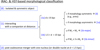 |
Fig. A.1. Schematic view of the morphological classification based on Spitzer/IRAC and HST images for the whole sample. |
Morphological and kinematic properties of the LIRG sample. The morphological classification is based on Spitzer/IRAC and HST/WFPC3 images. The kinematic classification is based on the ionized (Hα) and molecular (CO) gas kinematic maps according to the visual and kinemetry classifications. The final composite classification is also shown as a result of the combination of the two classifications.
Within the type 1 objects, we also defined other subclasses according to the distance involved in the system:
-
1a: interacting objects with a projected separation larger than 15 kpc; in cases where a symmetric morphology is seen (i.e., symmetric spiral arms), the galaxy is finally classified as ‘0’; otherwise, in the case of asymmetric morphology (e.g., asymmetric spiral arms), we confirm the morphological class as ‘1a’;
-
1b: interacting objects with a projected separation of between 1.5 and 15 kpc; if the interacting galaxies are characterized by similar mass we classify them as ‘1b major’, otherwise, if the masses are different we classify them as ‘1b minor’.
In some cases, the morphological classification alone could be misleading, and therefore we complemented this information with kinematic information available for the different gas phases (i.e., ionized and molecular). As mentioned in Sect. 1, the ionized emission (as traced by the Hα line) in our LIRG sample has been analyzed in previous works with the aim of studying the kinematic asymmetries in the Hα maps, through visual inspection (Bellocchi et al. 2013) and using the kinemetry method (Bellocchi et al. 2016). We report these results in Table A.1 (Cols. 4 and 5). Briefly, according to the visual classification we classify the objects as rotating disk (RD), perturbed disk (PD), and complex kinematics (CK) (see Bellocchi et al. 2013 for further details). According to the kinemetry method, we classify the galaxies as disk (D) or merger (M), and, when the galaxies belong to the “transition region”, as disk* (D*) or merger* (M*) (see Bellocchi et al. 2016 for details). The transition region is defined as the area where disks and mergers coexist, making their classification more uncertain. Furthermore, following the same scheme used for the Hα emission, we visually classify the kinematic maps produced for the molecular CO(2–1) line. These maps are not shown in this work, because this is beyond the scope of this paper; they will be presented in future works. However, these maps allowed us to better characterize the kinematics of our systems.
Combining both the morphological and kinematic information, we finally proposed the ‘composite’ classification shown in Table A.1 (Col. 7), defining the following classes:
-
0 (RD): single isolated objects, with relatively symmetric disk morphologies and without evidence for strong past or ongoing interaction. Their kinematic (i.e., velocity field and velocity dispersion) maps show the typical “rotating disk” pattern: i.e., point-antisymmetric velocity field and point-symmetric velocity dispersion (see Krajnović et al. 2006 for a detailed description; hereafter, rotating disk (RD));
-
0 (PD): single isolated objects, with relatively symmetric disk morphologies but showing a somewhat perturbed kinematics (perturbed velocity field and/or dispersion maps), suggesting past interactions (hereafter, perturbed disk (PD));
-
1: objects in a pre-coalescence phase with two well-differentiated nuclei separated by a projected distance of at least 1.5 kpc up to a maximum distance of 15 kpc (hereafter, interacting) showing perturbed or complex kinematics. Beyond this separation (> 15 kpc) the galaxies are also classified as ‘RD’ or ‘PD’, in a similar way to type 0 ones (e.g., ESO 297-G011/G012);
-
2: objects with two nuclei separated by a projected distance ≤1.5 kpc or a single nucleus with a relatively asymmetric morphology (e.g., tidal tail, asymmetric spiral arms), which suggests a post-coalescence merging phase (hereafter, merger). These systems show perturbed or complex kinematics.
In the specific case of NGC 2369, this is an isolated galaxy observed edge-on, showing a perturbed kinematics in Hα and CO. However, using the kinemetry method, it is classified as D*, then lying in the transition region: we proposed the ‘0 (PD)’ classification. NGC 5135 is an isolated face-on galaxy that shows quite complex kinematics in Hα and CO and is classified as D* with kinemetry. Furthermore, in this case, the Hα emission is perpendicular to the continuum emission. As in NGC 2369, we propose the classification ‘0 (PD)’. These are two extreme cases for which the perturbed and distorted kinematics might be due to the inclination effect of the sources: although the galaxies are isolated, in the face-on galaxy the rotational motion of the gas does not seem to clearly dominate the dispersion (v ≳ σ) while in the edge-on galaxy, projection effects could affect the observed velocity pattern.
Finally, IC 4687 belongs to a triple system and is the northern-most galaxy of the system. This source is separated by ∼10 kpc from the central galaxy (IC 4686) and by ∼30 kpc from the southern companion (IC 4689). The ratio of the dynamical masses between the northern (N), central (C), and southern (S) companions is 1 :  : 1 (N:C:S), allowing us to classify the NC system as ‘1b minor’. According to its kinematics, IC 4687 follows a relatively regular rotational pattern both in the ionized and molecular gas phases, and therefore we finally propose the ‘0 (RD)’ classification.
The visual kinematic classification proposed for our galaxies using the ionized and molecular gas tracers allowed a direct comparison between the two. Furthermore, the visual classification could also be useful to check the results obtained with kinemetry. Indeed, although this method allows us to quantify the asymmetries in the kinematic maps, the frontier which separates disks from mergers is not universal or clearly defined. This method therefore involves a certain degree of uncertainty in its classification.
For this reason, the final composite classification was carried out taking into account the morphological and kinematic information, in which the latter includes both the visual and the kinemetry classifications: this allowed us to analyze the sample under several aspects and finally draw more robust conclusions on the real nature of the systems.
Appendix B: CO(2–1) and 1.3 mm continuum ALMA maps and HST/NICMOS image
In this Appendix, we present the CO(2–1), 1.3 mm continuum flux density maps along with the stellar emission, observed using the near-IR HST/NICMOS F160W filter, for the whole sample.
We centered the CO(2–1) and 1.3 mm continuum images using the near-IR peak stellar emission. When the F160W filter is not available, other near-IR HST filters (e.g., F190W, F110W) are considered. When HST images are not available, the continuum peak emission at 1.3 mm is considered as a reference.
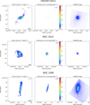 |
Fig. B.1. From left to right: CO(2–1) and 1.3 mm continuum maps obtained with ALMA, complemented by HST/NICMOS image when available. The CO(2–1) and 1.3 mm emission is > 5σ. The color bar is normalized to the maximum value of each ALMA map: in order to derive the real maximum value, a factor scale, shown in the top-right of each panel, has to be applied. The cross symbol in the three panels represents the stellar peak emission identified using the HST/NICMOS image. The beam size and the physical scale in kpc are also shown in the left panel. In all panels, north is up and east to the left. |
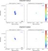 |
Fig. B.7. Same figure caption as in Fig. B.1 for the CO(2–1) and 1.3 mm continuum images, for which no HST/NICMOS data are available. The cross symbol identifies the continuum peak emission at 1.3 mm. |
Appendix C: CO(2–1) flux intensity maps ordered according to their increasing RCO
We present the CO(2–1) maps along with the 2MASS K-band maps for the whole sample. The maps are ordered according to the increasing molecular size, RCO. We used the same FoV for the whole sample (14 × 14 kpc2), both in the CO and stellar emissions for a more direct comparison. The effective radii of the molecular and stellar components are highlighted within the figures (Figs. C.1, C.2, C.3).
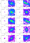 |
Fig. C.1. From top to bottom, left to right: CO(2–1) maps (left) and 2MASS images in the K band (right) of the whole sample. The galaxies are ordered according to their increasing RCO. The FoV is the same for all galaxies (14 kpc × 14 kpc). The black circle in each map identifies the respective effective radius in the map, whose value is also shown in each panel. North is up and east to the left. |
Appendix D: IR SED fit: ALMA flux loss estimation at 1.3 mm
In this Appendix we present the IR spectral energy distributions (SEDs) for the whole LIRG sample, using Herschel PACS and SPIRE data (Chu et al. 2017). The gray-body emission was derived assuming a β parameter of 2 (except for one case, IRAS F17138-1017) and one single gray body temperature, Tdust. The ALMA continuum fluxes at 1.3 mm are also shown but they have not been included in the fit. In all cases, the ALMA flux densities are below the SED fitting curve. We note that the total continuum flux emission was computed considering > 5σ emission.
The aim of this analysis is to quantify the flux loss derived when using ALMA data at 1.3 mm with respect to the extrapolated flux at 1.3 mm (through the SED fitting analysis). Indeed, at such frequencies (∼230 GHz), in addition to the dust emission we can also have some contribution from non-thermal synchrotron emission and thermal free-free emission (Condon & Ransom 2016). The ratio between the theoretical flux density and that obtained using ALMA is also highlighted in each fit. The gap between the two values clearly suggests that a considerable part of the 1.3 mm emission (< 70%) is not detected by our ALMA observations. The maximum recoverable scale is 3–5 kpc, and so extended diffuse and faint emission is unlikely to be filtered-out, but could be beyond the sensitivity of these data.
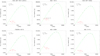 |
Fig. D.1. Spectral line energy distributions using Herschel data, assuming β = 2.0 and deriving the Tdust. The ALMA continuum flux at 1.3 mm at 5σ is also shown for a direct comparison. The ratio between the flux at 1.3 mm expected by the model and the ALMA value is also highlighted in red (Fratio). |
All Tables
Mean (and median) stellar mass Mstar, SFR, and sSFR for the different LIRG subsamples.
Molecular and 1.3 mm continuum effective radii determinations of the LIRG sample.
Mean (and median) half-light radius of the different tracers analyzed in the LIRG sample.
Mean (and median) half-light radius of the different tracers along with their stellar mass for local and high-z systems.
Ratios of the molecular, ionized and stellar ISM distributions of different types of galaxies relative to those of LIRGs.
Morphological and kinematic properties of the LIRG sample. The morphological classification is based on Spitzer/IRAC and HST/WFPC3 images. The kinematic classification is based on the ionized (Hα) and molecular (CO) gas kinematic maps according to the visual and kinemetry classifications. The final composite classification is also shown as a result of the combination of the two classifications.
All Figures
|
Fig. 1. Infrared luminosity versus redshift. The ‘composite’ classification is also shown according to the following color-code: in blue are represented the rotating isolated disk galaxies (0 (R)), in magenta the isolated perturbed disks (0 (P)), in green the interacting systems and in red the post coalescence mergers. Galaxies which belong to the same system (ESO 297-G011/G012, F12596 E/W and IC 4518 E/W) are identified using a solid line. Galaxies containing an AGN are identified by a square. |
| In the text | |
|
Fig. 2. LIRG sample in the SFR - Mstar and sSFR - Mstar planes. Left: SFR as a function of the stellar mass Mstar. The solid and dashed (orange) lines indicate the location of the local MS relation and the 1σ scatter, respectively, obtained by Elbaz et al. (2007) using SDSS galaxies at z ∼ 0 and converted to Kroupa IMF, in agreement with that derived by Whitaker et al. (2012). Our LIRGs are shown according to the color code defined in Fig. 1: isolated disks (RD), (PD), interacting, and merging systems are shown in blue, magenta, green, and red, respectively. The solid lines between the points (green and black) link galaxies that belong to the same system. Galaxies containing an AGN are identified with an empty black square. The horizontal red dashed line represents the threshold SFR to reach the LIRG IR luminosity (log LIR/L⊙ ≥ 11). Right: specific SFR as a function of the stellar mass Mstar. The three (solid, dotted, and dashed) gray lines identify the different SFR regimes (i.e., 1, 5, and 20 M⊙ yr−1, respectively). The MS relation is also shown (in orange). |
| In the text | |
|
Fig. 3. Histogram showing the distribution in physical scales (parsecs) of the size of the beam for the galaxies of the sample. The median and MAD values (solid and dashed magenta lines, respectively) correspond to 85 ± 18 pc. |
| In the text | |
|
Fig. 4. Relation between the CoG and A/2 results derived using VIMOS/VLT (Hα) data (Arribas et al. 2012). To derive this relation, close interacting pairs and the lower limits were excluded (see text). The dashed black line represents the 1:1 relation between the radii while the red solid line is the best fit. The plot shows the mean (standard deviation) and median (M) values of the RHα (CoG)/RHα (A/2) ratio. |
| In the text | |
|
Fig. 5. Paα image of the most extended galaxy of the sample, IC 5179, obtained from HST/NIC2 data (filters F187N and F190N). Gray contours highlight the regions in which the star formation is taking place. The FoV is about 19.5″ × 19.5″ with a FWHM ∼ 0.15″. North is up and east to the left. |
| In the text | |
|
Fig. 6. Relation between the observed (not corrected for extinction) Hα and Paα tracers when using A/2 and CoG methods applied to a subsample of 12 galaxies. Lower limits on Hα measurements are due to the limited FoV of VIMOS. Top panels: |
| In the text | |
|
Fig. 7. Left: CO(2–1) effective radius as a function of class. Type 0 (R), 0 (P), 1, and 2 are shown in blue, magenta, green, and red, respectively. The median RCO values (horizontal lines) are shown for each class. Empty squares identify galaxies containing an AGN. Middle:RCO distribution for the whole sample (gray solid line) and for the individual subgroups (same color code as in the left panel). The colored vertical lines in the upper part of the panel represent the median values of each distribution, following the same color code. Right:RCO distribution for the whole sample (gray solid line) and for LIRGs with an AGN. |
| In the text | |
|
Fig. 8. Left: SFR as a function of effective radius RCO. Galaxies containing an AGN are surrounded by a square. A Spearman’s rank correlation coefficient ρ = 0.32 is derived (see text). Right: stellar mass Mstar versus RCO (ρ = 0.53). The different types of galaxies are identified with the same color code as that used in Fig. 7. The orange solid line represents the best fit (linear least square fit). |
| In the text | |
|
Fig. 9. Effective radii derived for the CO(2–1) and Paα tracers using the CoG method. The black dashed line represents the 1:1 relation. The solid green line identifies the derived best fit to the data, which was derived using a linear least squares fit. Two outliers (IC 4687 and ESO 320-G030) are identified for which the RPaα ≳ RCO, while NGC 1614 is characterized by RCO ≳ RPaα. The most extreme RPaα is derived for IC 4518 E, and considered as an upper limit (see text for details). IC 5179 is a galaxy that shows similar effective radii for both gas tracers (RPaα ∼ RCO). |
| In the text | |
|
Fig. 10. Left: ionized gas size traced by the Hα emission, RHα, as a function of the stellar continuum size in the K band, Rstar. The 1:1 relation is shown using the dashed black line while the best fit is shown in magenta using a solid line; this latter was derived using a linear least square fit. The mean (standard deviation) and median (M) values are shown. Double circles represent galaxies containing an AGN. The dashed blue area represents the size covered by the CO emission for a direct comparison. Middle, right: molecular size versus stellar (middle) and ionized gas (right) distributions. The double circle identifies galaxies with an AGN. The dashed black line represents the 1:1 ratio. The solid lines and the shaded areas represent the median values (MAD). The mode values of these ratios are similar to the median values when considering the stellar results, while we derive a mode of ∼1.3 when considering the Hα results. |
| In the text | |
|
Fig. 11. Median effective radii (and MAD) derived for the different tracers and subsamples. The stellar, ionized, and CO(2–1) Reff are shown in magenta, green, and blue, respectively. Left: median values for the whole sample are shown (i.e., ‘ALL LIRGs’), along with the median values derived for the LIRG subsample with (w AGN) and without (w/o AGN) an AGN. Right: median Reff for the four subsamples defined in Table 1 (0(R) 0(P), 1, 2) are shown. |
| In the text | |
|
Fig. 12. Distribution of LIRGs and other low-z galaxy samples in the SFR–RCO (left), Mstar–RCO (middle), and sSFR–RCO (right) planes. Our LIRGs are shown according to the color code presented in Fig. 1. Local spiral galaxy (gray, red-contoured diamonds) values are taken from the EDGE-CALIFA survey (Bolatto et al. 2017) while ETGs (blue contoured, down-pointing triangles) are taken from the ATLAS3D sample (Cappellari et al. 2013a). ULIRG (purple pentagons) values are derived from ALMA data (Pereira-Santaella et al. 2021). The median value of each sample is shown according to the following color code: purple for ULIRGs, light green for interacting and merger LIRGs, light blue for disky (i.e., RD and PD) LIRGs, orange for spiral galaxies, and dark blue for ETGs. In ULIRGs, the AGN contribution has been removed to estimate their SFRs. |
| In the text | |
|
Fig. 13. Mass–size distribution for our LIRGs including ETGs and local spiral galaxies (i.e., MS SFGs; Leroy et al. 2021). ETGs are marked with (blue contour) down-pointing triangles and MS SFGs with up-pointing orange triangles. LIRGs are identified following the color code used in previous figures. The blue and red slopes represent the mass–size relations derived by Shen et al. (2003) (see also Fernández Lorenzo et al. 2013) for late- and early-type local galaxies, respectively. |
| In the text | |
|
Fig. 14. Mass–size distribution for our LIRGs and high-z galaxies (Table 6). LIRGs from this work are shown using light orange circles. High-z SFG and SMG data are taken from the following works: SMGs from Hodge et al. (2016), Chen et al. (2017), Calistro Rivera et al. (2018), and Lang et al. (2019) and SFGs from Barro et al. (2014), Straatman et al. (2015), Tadaki et al. (2017), Förster Schreiber et al. (2018), Cheng et al. (2020), Fujimoto et al. (2020), Kaasinen et al. (2020), Valentino et al. (2020), and Puglisi et al. (2021). The high-z data are shown following the color and symbol code shown in the legend. The blue and red lines in each redshift range represent the mass–size relations for late- and early-type galaxies, respectively, at z ∼ 1.75, 2.25, and 2.75 derived from the 3D-HST+CANDELS surveys (van der Wel et al. 2014). At z = 4 − 6, the mass–size relation for late- and early-type galaxies has not yet been derived, and so the dashed blue and red lines still show the behavior considered at z = 3 − 4. |
| In the text | |
|
Fig. 15. Ratios of different tracers in high-z (z = 2 − 2.5) galaxy samples relative to the low-z LIRG sample (Table 6). Left: stellar versus molecular size. Middle: stellar versus mm/submm (dust-) continuum size. Right: stellar versus ionized gas size. Our sample is shown using light orange circles, while the high-z galaxies are shown following the same symbol and color code shown in Fig. 14. In each panel, we report the references from which the high-z data are taken. Rmm cont derived for our LIRGs were derived from our 1.3 mm ALMA observations, which we considered as lower limits due to the limited sensitivity of our observations. |
| In the text | |
|
Fig. A.1. Schematic view of the morphological classification based on Spitzer/IRAC and HST images for the whole sample. |
| In the text | |
|
Fig. B.1. From left to right: CO(2–1) and 1.3 mm continuum maps obtained with ALMA, complemented by HST/NICMOS image when available. The CO(2–1) and 1.3 mm emission is > 5σ. The color bar is normalized to the maximum value of each ALMA map: in order to derive the real maximum value, a factor scale, shown in the top-right of each panel, has to be applied. The cross symbol in the three panels represents the stellar peak emission identified using the HST/NICMOS image. The beam size and the physical scale in kpc are also shown in the left panel. In all panels, north is up and east to the left. |
| In the text | |
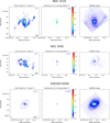 |
Fig. B.2. Same figure caption as in Fig. B.1 |
| In the text | |
 |
Fig. B.3. Same figure caption as in Fig. B.1 |
| In the text | |
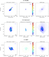 |
Fig. B.4. Same figure caption as in Fig. B.1 |
| In the text | |
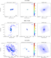 |
Fig. B.5. Same figure caption as in Fig. B.1 |
| In the text | |
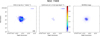 |
Fig. B.6. Same figure caption as in Fig. B.1 |
| In the text | |
|
Fig. B.7. Same figure caption as in Fig. B.1 for the CO(2–1) and 1.3 mm continuum images, for which no HST/NICMOS data are available. The cross symbol identifies the continuum peak emission at 1.3 mm. |
| In the text | |
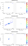 |
Fig. B.8. Same figure caption as in Fig. B.7 |
| In the text | |
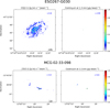 |
Fig. B.9. Same figure caption as in Fig. B.7 |
| In the text | |
|
Fig. C.1. From top to bottom, left to right: CO(2–1) maps (left) and 2MASS images in the K band (right) of the whole sample. The galaxies are ordered according to their increasing RCO. The FoV is the same for all galaxies (14 kpc × 14 kpc). The black circle in each map identifies the respective effective radius in the map, whose value is also shown in each panel. North is up and east to the left. |
| In the text | |
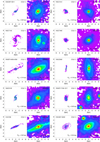 |
Fig. C.2. Same figure caption as in Fig. C.1. |
| In the text | |
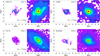 |
Fig. C.3. Same figure caption as in Fig. C.1. |
| In the text | |
|
Fig. D.1. Spectral line energy distributions using Herschel data, assuming β = 2.0 and deriving the Tdust. The ALMA continuum flux at 1.3 mm at 5σ is also shown for a direct comparison. The ratio between the flux at 1.3 mm expected by the model and the ALMA value is also highlighted in red (Fratio). |
| In the text | |
 |
Fig. D.2. Same figure caption as in Fig. D.1 |
| In the text | |
Current usage metrics show cumulative count of Article Views (full-text article views including HTML views, PDF and ePub downloads, according to the available data) and Abstracts Views on Vision4Press platform.
Data correspond to usage on the plateform after 2015. The current usage metrics is available 48-96 hours after online publication and is updated daily on week days.
Initial download of the metrics may take a while.