| Issue |
A&A
Volume 664, August 2022
|
|
|---|---|---|
| Article Number | A193 | |
| Number of page(s) | 27 | |
| Section | Interstellar and circumstellar matter | |
| DOI | https://doi.org/10.1051/0004-6361/202142531 | |
| Published online | 31 August 2022 | |
Probing the nature of dissipation in compressible MHD turbulence
Laboratoire de Physique de l’Ecole Normale Supérieure, ENS, Université PSL, CNRS, Sorbonne Université, Université de Paris,
Paris, France
e-mail: This email address is being protected from spambots. You need JavaScript enabled to view it.
Received:
27
October
2021
Accepted:
1
April
2022
Abstract
Context. An essential facet of turbulence is the space–time intermittency of the cascade of energy that leads to coherent structures of high dissipation.
Aims. In this work, we aim to systematically investigate the physical nature of the intense dissipation regions in decaying isothermal magnetohydrodynamical (MHD) turbulence.
Methods. We probed the turbulent dissipation with grid-based simulations of compressible isothermal decaying MHD turbulence. We took unprecedented care in resolving and controlling dissipation: we designed methods to locally recover the dissipation due to the numerical scheme. We locally investigated the geometry of the gradients of the fluid state variables. We developed a method to assess the physical nature of the largest gradients in simulations and to estimate their travelling velocity. Finally, we investigated their statistics.
Results. We find that intense dissipation regions mainly correspond to sheets; locally, density, velocity, and magnetic fields vary primarily in one direction. We identify these highly dissipative regions as fast and slow shocks or Alfvén discontinuities (Parker sheets or rotational discontinuities). On these structures, we find the main deviation from a 1D planar steady-state is mass loss in the plane of the structure. We investigated the effect of initial conditions, which yield different imprints at an early time on the relative distributions among these four categories. However, these differences fade out after about one turnover time, at which point they become dominated by weakly compressible Alfvén discontinuities. We show that the magnetic Prandtl number has little influence on the statistics of these discontinuities, but it controls the ohmic versus viscous heating rates within them. Finally, we find that the entrance characteristics of the structures (such as entrance velocity and magnetic pressure) are strongly correlated.
Conclusions. These new methods allow us to consider developed compressible turbulence as a statistical collection of intense dissipation structures. This can be used to post-process 3D turbulence with detailed 1D models apt for comparison with observations. It could also be useful as a framework to formulate new dynamical properties of turbulence.
Key words: magnetohydrodynamics (MHD) / magnetic reconnection / magnetic fields / turbulence / waves / shock waves
© T. Richard et al. 2022
 Open Access article, published by EDP Sciences, under the terms of the Creative Commons Attribution License (https://creativecommons.org/licenses/by/4.0), which permits unrestricted use, distribution, and reproduction in any medium, provided the original work is properly cited.
1 Introduction
Gravity drives the evolution of the Universe, but the gas dissipative dynamics is a central, yet unsolved, issue in the theories of galaxy and star formation (e.g. White & Rees 1978). An emergent scenario is that a large fraction of the gas internal energy is stored and eventually dissipated in turbulent motions of the coldest phases instead of being radiated away, and therefore lost, by the warmest phases (e.g. Guillard et al. 2012; Appleton et al. 2013; Falgarone et al. 2017). Turbulence, however, adds a colossal level of complexity to the gas dynamics, because cosmic turbulence is supersonic, involves magnetic fields, exhibits plasma facets, and pervades all the thermal phases. Moreover, its dissipation is known to occur in bursts localised in time and space, that is the space–time intermittency of turbulence (Landau & Lifshitz 1959; Kolmogorov 1962; Meneveau & Sreenivasan 1991).
Valuable and unexpected guidance in the investigation of the intermittent dissipation of interstellar turbulence is provided by a number of molecular observations, including the existence in the cold neutral medium (CNM) of specific molecules that require large inputs of supra-thermal energy to form (Nehmé et al. 2008; Godard et al. 2012) and of molecules more excited than an equilibrium at the ambient temperature would predict (Falgarone et al. 2005; Gry et al. 2002; Ingalls et al. 2011). The mere existence of large amounts of CO molecules surviving in irradiated diffuse media requires a formation route that is not controlled only by photons and cosmic rays (Levrier et al. 2012). This is in line with the large observed abundances of HCO+ in diffuse gas (Lucas & Liszt 1996; Liszt & Lucas 1998) now recognised observationally as a signature of supra-thermal chemistry (Gerin & Liszt 2021).
Supra-thermal chemistry can be driven by several processes that do not lead to turbulent dissipation bursts, such as the ionneutral drift in Alfvén waves (Federman et al. 1996), conduction at interfaces between the warm neutral medium (WNM) and the cold neutral medium (CNM; Lesaffre et al. 2007), transport between the WNM and CNM (Valdivia et al. 2017). These latter processes tap the reservoir of thermal energy of the WNM and are able to drive a warm chemistry in the CNM, but they fall short of reproducing the observed abundances of molecules with highly endothermic formation.
The channels linked to dissipation bursts, such as the ionneutral drift in C-type shocks (Flower et al. 1985; Flower & Pineau des Forets 1998; Draine & Katz 1986; Lesaffre et al. 2013) and in magnetised vortices (Godard et al. 2009, 2014), dissipative heating in shear layers (Falgarone et al. 1995; Joulain et al. 1998), shock heating, and compression (Lesaffre et al. 2020) tap the mechanical energy reservoir of the CNM, which is roughly of the same magnitude as the thermal energy reservoir of the WNM. However, they are naturally more successful because they can be much more concentrated in space, thus leading to potentially very strong effective temperature bursts. Out-of-equilibrium chemical and excitation signatures have been modelled for all these channels, which are related to specific localised structures where turbulent dissipation is enhanced. This detailed modelling is hard to reconcile with a coherent description of the energy cascade from the large scales of turbulence down to the dissipation scales, including intermittency. It has been attempted for the first time by chemical post-processing of state-of-the-art numerical simulations of MHD turbulence, including ion-neutral drift (Myers et al. 2015; Moseley et al. 2021). The smallest scales reached in these simulations are, however, far above the dissipation scales, but the results are promising. The subject of the present paper is to explore the nature, topology, and statistics of the dissipation structures that form in magnetised turbulence.
Turbulent dissipation has been extensively studied in incompressible media. In hydrodynamical (HD) turbulence, Moisy & Jiménez (2004) examined the geometrical properties of sites of extreme vorticity and shear. Uritsky et al. (2010) examined the statistical properties of sites of strong dissipation in incompressible magnetohydrodynamical (MHD) turbulence, and Momferratos et al. (2014) extended their work to include ambipolar diffusion (i.e. ion-neutral drifts). Zhdankin et al. (2013, 2014, 2015, 2016) extensively studied the statistics and dynamics of current sheets in reduced MHD. For example, Zhdankin et al. (2013) confirmed the Sweet-Parker view of reconnection, although they note that not all current sheets are involved in reconnection.
All the above studies were performed in an incompressible framework, while the interstellar medium is known to be extremely compressible. Here, we want to examine dissipation in the extreme case of isothermal turbulence, where thermal effects cannot help pressure to resist against compression. In the incompressible framework (see Momferratos et al. 2014, for example), the physical nature of a dissipation structure (current sheet or shearing sheet) is directly linked to the nature of the dissipation within this structure (it is either purely ohmic for current sheets or purely viscous for shearing sheets). The situation, however, is much more complicated in compressible HD turbulence, where shocks and shear can both lead to viscous dissipation, and even worse in compressible MHD, where dissipation structures can lead to viscous and resistive dissipation at the same place (as in a fast shock, see Lehmann et al. (2016) or our Appendix B).
Previous studies have attempted to characterise various individual types of structures. Smith et al. (2000a,b) investigated velocity jumps in the three main directions as a proxy to shocks. Yang et al. (2015) were able to single out and study the formation of one rotational discontinuity in a simulation of MHD turbulence. Lehmann et al. (2016) introduced the SHOCKFIND algorithm, which investigates an MHD snapshot to systematically extract every fast and slow shock. In the present study, we attempted to characterise the physical nature of all intense dissipation structures: we present a new improved method able to characterise fast and slow shocks as well as Alfvén discontinuities.
We wanted to examine the statistics of the various physical structures and their parameters and possibly assess how much dissipation is due to each category of dissipation structure. To this effect, we examined grid-based simulations of decaying isothermal MHD turbulence, which we present in Sects. 2.1 and 2.2. Because grid-based simulations are known to be more dissipative than pseudo-spectral simulations (which are, however, ill-suited to compressible fluids due to the Gibbs phenomenon), we devise and test a new method to retrieve the local dissipation intrinsic to the scheme (see Appendix B). Stone et al. (1998) investigated dissipation in driven and decaying MHD turbulence and concluded that about half of it is due to shocks. More precisely, they measured that 50% of the total dissipation is due to their artificial viscosity term. However, they did not account for implicit numerical dissipation, and they did not check whether their artificial viscosity was indeed located in shocks. Similar studies by Smith et al. (2000a,b, see their Table 1) also used artificial viscosity and suffered from the same uncertainties. Porter et al. (2015) and Park & Ryu (2019) did a much better job at detecting shocks and assigning dissipation to them but, their method still suffers from uncertainty when the shocks are not aligned with the grid, and it is restricted to shocks (it would not work for Alfvén discontinuities because they focus on density jumps). In the present work, thanks to our method of recovering the local dissipation everywhere (including the losses implicitly incurred by the numerical scheme), and because we carefully analyse the nature of intense dissipation structures, we hope to make more robust claims. For example, Lesaffre et al. (2020) performed a 2D HD simulation on such small scales that they were able to fully resolve the dissipation length scale and characterise almost all dissipation structures.
High dissipation is necessarily associated with strong variations of some of the variables controlling the physical state of the gas. We designed a technique to assess the main direction of the gradients of the physical state of the gas (Sect. 2.3). We observe that the regions of highest dissipation have their gradients locally and primarily in one direction (in other words, intense dissipation structures are sheet-like). We show how to decompose the gradients in this direction using a basis of MHD waves (Sect. 2.4). In Sect. 2, we examine the connected sets of pixels above a large threshold of dissipative heating and locally assess the nature of the physical profiles obtained by scanning along the main direction of the gradient. We tested whether the physical nature of these profiles agrees with the celebrated Rankine–Hugoniot (RH) relations (Macquorn Rankine 1870) and performed various consistency checks to confirm the physical nature of these scans. In Sect. 4, we examine the statistical properties of the scans we find. We discuss our results in Sect. 5 and conclude in Sect. 6.
2 Numerical Method
2.1 Simulation
In the present study, we ran a set of simulations of decaying magnetohydrodynamics (MHDs) turbulence.
2.1.1 Numerical Method
We solved the evolution equations of resistive and viscous isothermal MHDs, which we write here in conservative forms:
 (1)
(1)
![Mathematical equation: $ 0 = {\partial _t}\rho {\bf{u}} + \nabla \cdot \left( {\rho {\bf{uu}} - v\rho {\bf{S}}\left[ {\bf{u}} \right]} \right) + \nabla p - {\bf{J}} \times {\bf{B}}, $](/articles/aa/full_html/2022/08/aa42531-21/aa42531-21-eq2.png) (2)
(2)
 (3)
(3)
where ρ is the mass density, u is the fluid velocity vector, p = ρc2 is the thermal pressure with c as the isothermal sound speed, B is the magnetic field, and  is the current vector. v and η are, respectively, the viscous and resistive coefficients. The components of the viscous stress tensor S are expressed as
![Mathematical equation: $ {S_{ij}}\left[ {\bf{u}} \right] = {\partial _i}{u_j} + {\partial _j}{u_i} - {2 \over 3}{\partial _k}{u_k}{\delta _{ij}}, $](/articles/aa/full_html/2022/08/aa42531-21/aa42531-21-eq5.png) (4)
(4)
where ∂i denotes the derivative with respect to the space coordinate i.
To integrate these equations, we used the code CHEMSES (Lesaffre et al. 2020), which originates from DUMSES (Fromang et al. 2006), a version of RAMSES (Teyssier 2002) without adaptive mesh refinement. The ideal part of the evolution step is evolved thanks to a Godunov scheme with a Lax-Friedrichs Riemann solver and a minmod slope limiter function (see Toro 1999 for more details). The magnetic field is evolved with constrained transport to preserve its zero divergence (Fromang et al. 2006). This ideal MHD step is sandwiched between two half dissipation steps to preserve the second-order accuracy of the time integration (see Lesaffre et al. 2020 for more details). CHEMSES inherits the centring of the RAMSES code, with densities and velocity components at the centre of cells and magnetic field components at the centre of their respective cell interfaces (Fromang et al. 2006). The resistive and viscous stresses are centred accordingly, and a diffusion estimate (for both viscous and resistive dissipation) replaces the reference Courant time step whenever it is shorter. For example, the viscous diffusion time step constraint is ∆τ = (∆x)2/(6v), where ∆x is the pixel size. We set the Courant number1 at the value of 0.7 throughout all the simulations of the present work. For an isothermal gas, the viscous coefficient v should be such that μ = ρv is a constant; indeed, v scales as the sound speed times the mean free path, which itself scales as 1/ρ. However, we still used a constant kinematic viscous coefficient v as in Federrath (2016) rather than a constant dynamical viscosity μ = ρv, as this allows easier numerical convergence for shocks (see Appendix B).
2.1.2 Initial Conditions
The quantities computed in the code are dimensionless. They are normalised by physical scales set such that the average square velocity is initially 〈u2〉 = 1, the cubic domain size is L = 2π, and the average density 〈ρ〉 = 1, where the brackets denote averages over the whole simulated domain. The non-dimensional value of the isothermal speed c thus controls the r.m.s. initial sonic Mach number as ℳs = 1/c. The initial density is uniform, and the initial magnetic field is scaled to obtain  so that the effective r.m.s. initial Alfvénic Mach number is equal to 1, as well as the r.m.s. initial Alfvén speed (cA). We note that the mean magnetic field is zero over the computational domain. For example, imagine one wants to apply these results to a physical region of physical dimension ℓ of r.m.s. velocity ur.ms. and average density ρav. Then, dimensionless quantities in the code can be converted to physical quantities according to xphys = ℓ/(2π) · x for distances, uphys = ur.m.s. · u for velocities, and
  for magnetic fields.
As in Momferratos et al. (2014), we considered a periodic box with initial conditions based either on the Arnol’d–Beltrami–Childress (ABC; see Bouya & Dormy 2013, e.g.) flows or on the Orszag–Tang vortex (OT; Orszag & Tang 1979). For the ABC flow, the velocity field is set by a superposition of sines and cosines:
 (5)
(5)
where A, B, and C are coefficients chosen for the three smallest wave numbers k (largest scales) from a uniform number generator in the interval [−1, 1]. For smaller scales, a random field uE is added, with the following energy spectrum:
 (6)
(6)
where kc = 3, and CE is chosen so that  . This random field is set in Fourier space with the amplitude of the complex coefficients prescribed by the above spectrum, and the phase of each coefficient is drawn from a uniform distribution in the interval [0, 2π]. The perturbed initial ABC velocity field u = α(uABC + uE) is rescaled so that 〈u2〉} = 1 by properly setting α. The initial magnetic field for the ABC runs is set with a random field drawn in a similar way to uE. The power spectrum of the initial random perturbation is a minimal seed to initiate a cascade and let it develop naturally. Indeed, we want our results to testify for our large-scale initial conditions rather than for the added seed. We hence chose its logarithmic slope to be significantly steeper than the expected Kolmogorov (k−5/3) or supersonic (k−2, see Federrath 2013; Federrath et al. 2021) spectra, with an additional exponential cut-off for safety.
The OT vortex velocity is defined by
 (7)
(7)
to which we also add random perturbations as in the ABC case. The initial magnetic field for the OT vortex is set as
 (8)
(8)
without additional perturbation. The velocity and magnetic fields are then rescaled so that  .
.
Our ABC flows have a significant magnetic helicity  , where A is the potential vector, and B = ∇ × A with Coulomb gauge divA = 0) and an almost zero cross helicity
  . That means the magnetic field is topologically complex and there is no strong correlation between magnetic and velocity field. For OT initial conditions, the situation is reversed, it has an almost null magnetic helicity and a non-zero cross-helicity (see Table 1 for the values of helicities).
In addition to the initial conditions, we also investigated the resolution. Our fiducial runs have a number of pixels N = 1024 per side of the cubic computational domain, and we degraded the resolution by a factor two to control the stability of our results. We also probed the effect of varying the Prandtl number Pm = v/n. Table 1 summarises the parameter space we covered.
2.2 Dissipation Recovery and Control
The numerical scheme we used (Godunov) implicitly introduces dissipation to evolve the ideal MHD equations, but, as stated above, we incorporated additional explicit physical dissipation terms in our evolution equations. It is important to retain some amount of physical viscosity as Godunov schemes do not provide an implicit viscosity in shear layers. Here, we discuss our methods used to estimate the fraction of the dissipation due to the numerical scheme.
We set values for the viscous and resistive coefficients v and η identically to those used by Momferratos et al. (2014) in pseudo-spectral simulations with 5123 spectral elements: v = η = 7 × 10⁻⁴ in the same non-dimensional units. This is motivated by the common belief that spectral codes are approximately twice as efficient as grid based codes. Our study for shocks in Appendix B presents a more detailed picture. Figure B.1 shows the dissipation bump in a fiducial shock front at various resolutions. For our chosen values for the dissipative coefficients and a resolution of N = 1024, we see it is effectively spread up by nearly a factor of three, while one would have to increase the resolution by a factor of eight to fully resolve it. A resolution two times smaller would spread the front by a factor of six, and thus our current choice is a good compromise between accuracy and CPU efficiency.
In isothermal MHDs, the integrated total isothermal generalised mechanical energy  ) decreases due to all irreversible processes taking place (see Eq. (B.3)). Because our Godunov time integration scheme features a conservative round-off error, we can use its time derivative to estimate the global budget of dissipated energy:
 (9)
(9)
where 〈εtot〉) is the total rate of irreversible heating integrated over the whole computational domain. Appendix B presents and tests a new method to estimate the total irreversible heating εtot locally. The chosen method has the additional advantage that it preserves the round-off error of the validity of Eq. (9) when integrated over the whole domain.
We can now decompose the local total heating rate as
 (10)
(10)
where
![Mathematical equation: ${\varepsilon _\nu } = \rho \nu {S_{ij}}\left[ {\bf{u}} \right]{\partial _i}{u_j}$](/articles/aa/full_html/2022/08/aa42531-21/aa42531-21-eq21.png) (11)
(11)
and
 (12)
(12)
are the local viscous and resistive dissipative heating rates, and εnum is the dissipation due to the numerical scheme.
We can then estimate the local numerical dissipation rate simply by computing εnum = εtot − (εv + εη), where we use well-centred estimates for Eqs. (11) and (12). If our estimate for the local dissipation were perfect, this quantity would always be positive, because we are performing our simulations with a time step small enough for the scheme to be stable (it is set to 70% of the shortest unstable time step). However, we are subject to truncation errors in both the εtot term (see Appendix B) and the εv + εη terms (where a centred difference is used). The difference between the two terms can hence be negative due to these truncation errors. We thus define  as a corrected local total dissipation rate, which ensures the resulting estimate for εnum is positive. It is equal to the total local dissipation εtot where the numerical dissipation is positive (i.e. where εtot > (εv + εη)), while it is equal to the total physical dissipation εv + εη elsewhere. This ensures the corrected local numerical dissipation rate
  is always positive. In particular, the local corrected total dissipation rate
  is always greater than εtot. It is then shared between resistive and viscous natures in the same proportions as the physical terms we introduced to provide estimates for viscous and resistive dissipations including numerical dissipation:
 (13)
(13)
 (14)
(14)
Figure 1 displays the temporal evolution of various total dissipation rates. Thanks to the equality in Eq. (9), we can compute the exact total dissipation rate at each time step (blue curves), and we can compare it to the integrated local estimate  (green curves), which by construction is always greater. The difference between the two gives an estimate of the error we make on the estimation of the dissipation (of the order of 1% at most). It corresponds to the integrated estimated εnum in all the pixels where it is negative. The orange curves show the integrated physical dissipative terms 〈εv + εη〉. They amount to about two thirds of the total, while the remainder is numerical dissipation by the scheme.
Parameters of simulations we analysed.
2.3 The Local Frame of Physical Gradients
We know local intense dissipation events are caused by strong variations of some of the fluid state variables. Here, we want to identify regions where the fluid state varies strongly and characterise its variations in each direction.
The fluid state is characterised by the seven (1 + 3 + 3) components of W = (ρ, u, B), which do not have the same physical dimensions. We want to put the variations of density, velocity and magnetic fields on equal footing. Hence, we need to rescale the gradient of each component of W to make them homogeneous to the same physical dimension. We now choose to define the rescaled gradient of W in a given direction r as
 (15)
(15)
where  is the unit vector in the direction of r. This rescaled gradient has the dimension of the inverse of a length scale, which represents the typical length scale over which the state variables vary in the direction
  .
.
The norm of this gradient will be large whenever there is a rapid change in one or several state variables. Its square can be expressed as
 (16)
(16)
where αij = ∂iW · ∂jW is a 3 × 3 matrix (and the dot product applies to the seven components’ vectors) with coefficients homogeneous to an inverse squared length. It is real, symmetric, and therefore diagonal on an orthonormal basis. We can rewrite Eq. (16) in a more explicit form:
 (17)
(17)
where  , and
, and  are the inverse of the eigenvalues associated with the eigenvectors
  , and
, and  of the matrix αij. Equation (17) shows how the gradient of state variables depends on directions. A 3D polar plot of the norm of this gradient takes the form of an ellipsoid whose principal axes are in the three orthogonal eigenvalue directions of the above matrix:
 (18)
(18)
with the three length scales ordered so that ℓscan ≤ ℓ⊥1 ≤ ℓ⊥1. These three variation length scales and their associated orthogonal directions characterise the local geometry of the gradients of the fluid state variables.
Figure 2 shows how the aspect ratios between these typical variation length scales are distributed in all cells of a simulation (left panel) and only for highly dissipating ones (four standard deviations over the mean, right panel). It shows that most fluid state variables vary primarily in one direction for extreme dissipation events, whereas aspect ratios span all possibilities if we consider the full simulation domain. We also notice a slight imbalance towards ribbons compared to sheets. When one variation direction is dominant (ℓscan ≪ ℓ⊥1 ≤ ℓ⊥1), quantities are essentially constant in the direction orthogonal to it, and the local situation is hence nearly a ID plane parallel. We thus define the planarity as the ratio ℓ⊥1/ℓscan, which is large whenever ℓscan ≪ ℓ⊥1, i.e. when the local geometry is close to plane-parallel.
This ID geometry of gradients for intense dissipation regions is consistent with the typical two-dimensional geometry of the structures found in MHD turbulence (Uritsky et al. 2010; Zhdankin et al. 2013; Momferratos et al. 2014). On intense dissipation structures, we should thus be able to capture most fluid variations by browsing those in the maximum gradient direction. As described in Sect. 3.2, we used  as a sampling direction to probe the variation of physical quantities around strong dissipation regions.
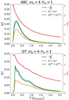 |
Fig. 1 Time evolution of volume-integrated dissipation rates for the ABC and OT, Pm = 1 runs. The blue line is the time derivative of the integrated isothermal generalised mechanical energy |


2.4 Gradient Decomposition into MHD Waves
In the ideal case where the gradient would be strictly in one direction, the gas dynamics are governed by ID plane-parallel MHD equations, and we show here how local gradients can be projected onto ideal MHD waves.
We write x the space coordinate along the direction of the gradient and t the time coordinate. The requirement ∇ · В = 0 implies that ∂xBx = 0. The corresponding component of ∂xW is thus zero. It turns out that the six non-zero components of ∂xW are spanned by the six ideal MHD waves, which we now explain.
Wave solutions take the form W(x, t) = F(x − υt), where υ is the travelling speed of the wave. We note that ∂tF = −υ∂xF and plug this form into the ideal MHD part of the equations (without the dissipation terms). We arrive at a linear eigenvalue problem for which we can find six eigenvectors ∂xF, with eigenvalues υ corresponding to the six waves of ideal isothermal MHD2. We label them by their wave type, s, i, or f, for slow, intermediate, or fast, and their direction of propagation RorL for right (or forward, υ > 0) and left (or backward, υ < 0). To within a multiplicative constant, the expressions for intermediate waves for these eigenvectors are (see Sect. 5.2.3 of Goedbloed et al. 2019 or Sect. 6.5 of Gurnett & Bhattacharjee 2005, for example)
 (19)
(19)
where ϵR,L = −1 for left-travelling (backward going) waves and ϵR,L = 1 for right-travelling (forward going) waves,  is the Alfvén velocity vector, at, is the transverse component of α, αx is its x-component, and
  is at, rotated by π/2 in the transverse plane. The first component of this gradient is zero, and hence the density is uniform. The transverse magnetic field has its gradient orthogonal to itself, meaning that it rotates along the scanning direction. The corresponding travelling speed is
  .
.
The expressions for fast and slow magnetosonic waves are
 (20)
(20)
where the propagation speed  reads
reads
 (21)
(21)
with  and ϵf,s = 1 for fast waves or −1 for slow waves. These waves are compressive (the density gradient is nonzero) and the gradient of transverse magnetic field is aligned with itself. In other words, the transverse magnetic field remains in the same direction, which also happens to be the same direction as the variation of the transverse velocity. Both the velocity and the magnetic field vectors thus remain in the plane defined by the scanning direction x and the initial transverse field (a property sometimes referred to as the coplanarity of these waves).
These six gradients form an orthogonal basis that can be easily normalised to make it an orthonormal basis  . Any gradient
  can now easily be decomposed into the six waves by computing the scalar product
  . Thanks to orthonormality, we have
  , and each coefficient
  can be interpreted as a 0-to-1 coefficient that characterises how similar the gradient
  is to the corresponding ideal MHD wave. We define the ‘most representative wave’ as the wave with the largest coefficient in this decomposition. The most representative wave characterises the local gradient as slow, intermediate, or fast, each one in a left- (backward) or right- (forward) travelling version depending on the sign of its speed relative to the fluid
  . We also note that this decomposition does not change if we add a constant vector to the velocity; it is independent of the choice of Galilean frame.
Until now, we have only considered wave solutions of the ideal part of the MHD equations (without dissipation), while the gradients in our simulation result from the evolution of fully dissipative MHD. We now consider a non-linear wave solution of the ID, fully dissipative MHD Ffull(х − υfullt) such as the isothermal shocks of Appendix A. The profile of this wave continuously joins two uniform states related by the Rankine-Hugoniot relations (see Sect. 3.3). These two states are separated by a region where dissipation occurs. We consider the gas state at the local maximum of dissipation; this is where the gradients of the state variables are the largest, and where the gradient of viscous and resistive stresses are likely to be small (because we are close to their maximum). At this position, the ID dissipative physics behaves as the ID ideal physics, and we can expect that the measured gradients fall along one of the ideal wave gradients we described above. As a result, the fully dissipative wave speed should be well approximated by its ideal estimate:  where ux is the fluid velocity and
  applies to the most representative wave at the dissipation maximum. We make use of this fact in the following to estimate the steady-state velocity of the structures we detected (see Sect. 3.3.2). Furthermore, we investigated the gradients of semi-analytic isothermal shock profiles (computed in Appendix A) and we noticed that gradients in slow shocks are dominated by slow magnetosonic waves all along their profiles. Similarly, fast shocks gradients are dominated by fast magnetosonic waves. This result seems natural, but we find it nevertheless surprising that dissipative physics does not affect the nature of gradients more, and we have not yet found a satisfactory explanation for this behaviour.
Finally, we note that we can always decompose a gradient in a given direction, but it makes less sense if the 3D gradient is not strongly dominated by a single direction. By selecting intense dissipative cells, however, we are more likely to be in a situation where the gradient is well directed (see Fig. 2 and previous subsection).
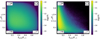 |
Fig. 2 2D joint probability density function of gradients’ aspect ratios (for the OT simulation at Pm = 1 at time t = tturnover/3). On the left, characteristic lengths are calculated for all the simulation cells. While on the right, the domain is restricted to cells where |

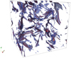 |
Fig. 3 Intense dissipation structures extracted from an OT initial conditions simulation with Pm = 1. The time step of this output is t ≃ 1/3tturnover. Structures are shown through dissipation isocontours. The first one, in blue, is set at |

3 Dissipation Structures
3.1 Definition and Visualisation
In turbulent MHD flows, the bulk dissipation of kinetic and magnetic energy occurs in a small volume compared to the global scale of the flow. Dissipation has been analysed and observed in several studies (e.g. Uritsky et al. 2010; Zhdankin et al. 2013; Momferratos et al. 2014) to be organised in ribbon-shaped or sheet-like coherent structures.
Figure 3 shows isocontours of the total dissipation rate  . The dissipation rate in each cell is computed using the method described in Appendices A and B. We followed previous work (Uritsky et al. 2010) and defined a connected dissipation structure as a connected set of cells, where
 (22)
(22)
with λ being a parameter we used to tune the detection threshold,  the dissipation rate determined by our method, and
  the standard deviation of the dissipation rate distribution. We chose λ = 4 because we find that energy transfers are mainly due to events above 4σ; we checked that the bulk of the third-order structure function (responsible for energy transfers) was obtained from increments above 3–4 sigma. We also wanted the structure to be identifiable as clearly as possible, and we expect such high dissipation structures to be associated with more intense gradients and a more clear-cut physical nature.
As already hinted by local gradients (Fig. 2), we see in Fig. 3 that extracted dissipation structures are mainly sheets. Another way to see this is to look at a thin slice of the dissipation field in our OT simulation with Pm = 1 (Fig. 4), where the trace of the sheets appears as thin ridges. Compared to the same figure for the incompressible runs of Momferratos et al. (2014), the viscous and ohmic natures of dissipation are now much more entangled and sometimes even overlap. A close eye inspection of this figure (and of similar cuts at other time steps and initial conditions) reveals various sub-layering of ohmic dissipation sheets (red striations or ohmic dissipation wrapped by shear) or isolated viscous and ohmic heating sheets (purple in colour, which hints at a mix of compressive viscous heating and ohmic heating). These are not the only situations to occur, but it reveals that the intense dissipation sheets are not always randomly positioned with respect to one another.
A careful inspection of Fig. 3 allows us to witness a few small, filament-like structures. Some of them may be traced on Fig. 2 by the low-probability tail in the bottom right hand corner of the right panel, where the aspect ratios of the gradients are such that ℓscan ≃ ℓ⊥1, while ℓ⊥1 ≫ ℓ⊥2. These tube-like structures will unfortunately be missed by our systematic investigation, which focuses on locally planar structures, but we checked, a posteriori, that these structures only account for a very small fraction of the dissipation (less than 1%).
Figure 5 shows how the dissipation is distributed in volume. It gives the volume filling factor of the regions of large dissipation as a function of their dissipation fraction. This figure compiles several time steps up to t = 1.33tturnover, where  is the initial eddy turnover time. It shows that the intermittency of the dissipation decreases over time as the r.m.s. sonic Mach number decreases, because we considered decaying turbulence simulations (Fig. 1 shows the rapid decline of the sonic Mach number). We see here that structures shown in Fig. 3 (yellow lines for dissipation greater than four standard deviations above the mean) occupy ≃0.8% of the volume, while they are at the origin of ≃25% of the total dissipation rate.
As we used decaying simulations, the Mach number and dissipation decrease rapidly. We considered snapshots at two characteristic times. The first snapshot is at 1/3 of the turnover time, when the first large dissipative structures form, and shortly after the dissipation peak. It is customary to think of the dissipation peak as a point similar to a steady state, because the time derivative of the dissipation is zero. However, as we show, this epoch still bears a strong imprint from the initial conditions. We therefore also considered a second snapshot at one turnover time. We did not consider much later times, as turbulence quickly decays and r.m.s. Mach numbers become much lower than at the beginning (see Fig. 1).
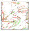 |
Fig. 4 Dissipation cut at time t = 1/3tturnover for OT initial conditions with Pm = 1. Lower and upper thresholds have been applied to the 3% pixels with smallest and largest dissipation, the intensity scaling of the pixels is logarithmic, while the colour-code is as follows. Red: ohmic dissipation εη = 4πηJ2; blue: compressive viscous heating εcomp = 4/3pv (∇ · u)2; green: solenoidal viscous heating εsol = ρv (∇ × u)2. We warn the reader that |

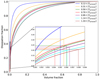 |
Fig. 5 Dissipation filling factor for a simulation with OT initial conditions that started at ℳs = 4. Each solid-coloured curve gives the total dissipation corresponding to the fraction of the volume occupied by the most dissipative regions for different time steps. Vertical dashed lines mark the volume occupied by the selected threshold for the structure detection ( |
3.2 Identification of Structures
We develop on the details of our procedure to identify scans along the connected structures.
3.2.1 Scanned Profiles
We considered each connected dissipation structure one at a time. In a selection of cells (see our selection strategy in Sect. 3.2.5), we took  as a scanning direction on which we sampled the magnetic field, fluid velocity, density, and total pressure
 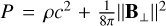 , where B⊥ is the magnetic field transverse to the scanning direction. We note that we do not include the contribution to the total pressure of the magnetic field component in the scanning direction, because it should remain uniform in this direction. We linearly interpolated their values every 0.2 cell side lengths (this is to avoid accuracy asymmetries resulting from the staggered position of the magnetic field components). As in SHOCK_FIND (Lehmann et al. 2016), each value was then averaged over a three-cell radius disc, orthogonally to the scanning direction. This smooths profiles and makes our identification less sensitive to the orientation of the scanning direction with respect to the cell edges. Four representative scans are displayed in Fig. 6.
3.2.2 Pre- and Post-Positions
To identify each side of the discontinuity causing the dissipation peak, we define reference positions pre- and post-discontinuity. To do so, we examined the total dissipation profile in the scan direction (Fig. 6, second row), and we estimated the local scale of variation of dissipation ℓε by fitting a parabola on log  over two cell lengths. The resulting scale ℓϵ is usually between two and four cells in length. We adopted ±3ℓε as a good compromise: not too close to the dissipative layer so that the dissipative terms are negligible and not too far away so that the dynamics is still dominated by the discontinuity.
To improve the reliability of our identification criteria, we allowed ourselves to change the sign of the director vector rscan. We adopted the direction in which the total pressure and density increases from pre- to post-discontinuity. The sign of r⊥1 was modified to keep a right-handed coordinates system. If density and total pressure variations are opposite, we then chose the direction of propagation of the dominant ideal wave in the gradient decomposition in ideal waves presented in Sect. 2.4.
3.2.3 Heuristic Criteria
We first designed three categories according to the classical MHD shock type classification derived from Rankine–Hugoniot (RH) jump conditions: fast shocks, slow shocks, and Alfvén discontinuities (see Sect. 3.3). We defined three heuristic criteria to sort the resulting profiles into these categories.
The category of fast shocks (H1) is characterised by a total pressure increase and a transverse magnetic field increase. The category of slow shocks (H2) is characterised by the increase in density and the decrease of the transverse magnetic field. The category of Alfvén discontinuity (H2) is characterised by a density bump and a trough in transverse magnetic field.
To determine the variation of the profiles, we compared the values of the pre-discontinuity, peak dissipation, and post- discontinuity positions, and each of these values was averaged over a one-cell side window to avoid spurious variations. By ‘increase’ and ‘decrease’, we mean that the variation is mono-tonic across these three positions, while by ‘bump’ (resp. ‘trough’) we mean the central value is above (resp. below) the other two positions.
For shock identifications, the total densities and pressures must increase. However, for fast shocks, the jump in density is small compared to the jump in total pressure. In some cases, the uncertainty on the position of the post-shock could lead to a non-identification if the relaxation of the post-shock pressure to that of the ambient medium is fast enough. This is why we do not consider a density rise as a reliable criterion for fast shock identification. Slow shocks are the opposite case; the total pressure jump is small compared to the density jump. We thus did not include the total pressure increase criterion to identify them. Profiles that do not fall into any of the categories are flagged as unidentified.
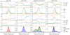 |
Fig. 6 Representative scan profiles used to identify the different kinds of dissipation structures in our simulations (here, for the ABC simulation at Pm = 1 at time t = tturnover/3). The first four rows of plots show, respectively, velocities (in the local velocity frame of the scan, and normalised by the initial r.m.s Alfvén speed), dissipation rates, density and total pressure, and magnetic field components’ profiles. The last row shows gradient decomposition into ideal waves. The coloured surfaces in between the curves is proportional to the weight of each corresponding ideal wave (in the decomposition presented in Sect. 2.4). Vertical dashed lines on each plot mark the positions of pre- and post-discontinuity that we define in Sect. 3.2.2. |
3.2.4 Gradient Decomposition Criteria
We now supplement these heuristic criteria by using the gradient decomposition method described in Sect. 2.4. Gradient decomposition is another method used to locally characterise the nature of the variations of gas-state variables across discontinuities. The use of this technique on the analytical profiles of ID isothermal fast and slow shocks (as computed in Appendix A) shows us that they decompose into almost pure fast and slow magnetosonic waves, respectively. We have no prior information on the wave decomposition of Alfvén discontinuities, but we find that profiles corresponding to our heuristic criteria for Alfvén discontinuities yield two exclusive cases; they either decompose mostly into intermediate waves, or they decompose mostly into slow magnetosonic waves.
For the specific case of a transverse magnetic field inversion (i.e. the transverse magnetic fields are opposite each other on the pre- and post-sides of the profile), we find there are two possible ways for it to go from one side to the other side. It can either rotate continuously until reaching the angle π, or it can use a co-planar path by shrinking until it vanishes and then expand in the other direction. These two situations cannot be distinguished via pre- and post-discontinuity values alone, as in the classical view of Rankine-Hugoniot relations. The difference resides in the internal structure of the discontinuity itself, with a rotation in one case (which has a gradient decomposition dominated by intermediate waves) and in the other case a co-planar variation of the transverse magnetic field (for which we find a gradient decomposition dominated by slow magnetosonic waves).
For each scan, we thus estimate the relative weight of each type of ideal wave decomposition averaged over the scan as
![Mathematical equation: ${{\cal F}_{s,i,f}} = {{\int_{{s_{{\rm{pre}}}}}^{{x_{{\rm{post}}}}} {{\rm{d}}x\left[ {{{\left( {{\bf{\hat e}}_{s,i,f}^R.{\partial _{{\bf{\hat x}}}}{\bf{W}}} \right)}^2} + {{\left( {{\bf{\hat e}}_{s,i,f}^L.{\partial _{{\bf{\hat x}}}}{\bf{W}}} \right)}^2}} \right]} } \over {\int_{{x_{{\rm{pre}}}}}^{{x_{{\rm{post}}}}} {{\rm{d}}x{{\left\| {{\partial _{{\bf{\hat x}}}}{\bf{W}}} \right\|}^2}} }},$](/articles/aa/full_html/2022/08/aa42531-21/aa42531-21-eq71.png) (23)
(23)
where subscripts s, i, and f stand for slow, intermediate, or fast. x is the position along the scanning axis. xpre and xpost are the pre- and post-discontinuity positions, respectively. We note that  .
.
Our identification criteria take into account the agreement between the heuristic and the ideal wave gradient decomposition methods. We therefore only define structures that show an agreement between the two methods as identified. According to these criteria, H1 heuristic (see Sect. 3.2.3) and fast wave-dominated gradients ( and
and  ) are the fast shocks. While slow shocks are identified with H2 heuristic and slow wave-dominated gradients (
 and
and  ). The Rotational discontinuities are characterised by heuristic H2 and slow wave-dominated gradients (
 and
and  ). The Parker sheets, on the other hand, exhibit H3 heuristic and slow wave dominated gradients (
 and
and  ).
).
Representative example profiles of the four kinds of dissipative events we encounter are shown in Fig. 6. For some profiles, the dominant wave weight does not correspond to the heuristic type. We flag these as misidentified. Finally, we note that our divide between rotational discontinuities and Parker sheets may be arbitrary. We found no metric in which the statistics for these two classes clearly separate (i.e. with a gap between them), and there are, on the contrary, many indications that they just form the two sides of a continuum of Alfvén discontinuities.
3.2.5 Scanning Strategy
We examined each connected dissipation structure one at a time. We sorted the cells of a given structure by decreasing planarity (ℓ⊥1/ℓscan) to obtain the most reliable identification (the most planar cells are scanned first). To prevent overlap of integration domains and to save computation time, once a scan was not identified, we removed cells around it from the remaining cells to be identified. We remove all the cells that belong to a rectangle parallelepiped, whose square faces are orthogonal to the scan axis and have a side length of 20 cells. We then examined the next most planar cell in the remainder of the structure until we exhausted all cells for that structure. Once we had considered all available structures in the computational domain, we were left with a list of scans and their identifications, the statistics of which we discuss in Sect. 4.
3.3 Rankine–Hugoniot Validations
Rankine–Hugoniot (RH) relations express jump conditions across discontinuities in their stationary frame (Macquorn Rankine 1870; Gurnett & Bhattacharjee 2005). RH relations hold in a very specific situation where the fluid is stationary, with a plane-parallel symmetry and homogeneous conditions on either side of a discontinuity. Nothing seems further away than our fully turbulent decaying turbulence simulations. Nevertheless, we wanted to check if our structure identification would allow us to recover some of the properties expected from the RH relations. If they held, it would bring more weight to the selection criteria we devised, and it would generalise the results of Lesaffre et al. (2020) to 3D MHD. They found that in 2D, decaying, unmagnetised turbulence, 1D steady-state shocks could be used to model the strongest dissipation structures. In 1D, steady-state, isothermal MHD, conservation of mass, momentum, and magnetic field read
![Mathematical equation: $\left[ {\rho {\bf{u}} \cdot {\bf{n}}} \right]_{{\rm{pre}}}^{{\rm{post}}} = 0,$](/articles/aa/full_html/2022/08/aa42531-21/aa42531-21-eq81.png) (24)
(24)
![Mathematical equation: $\left[ {\rho {\bf{u}}\left( {B \cdot {\bf{n}}} \right) + \left( {p + {{{B^2}} \over {8\pi }}} \right){\bf{n}} - {{\left( {{\bf{B}} \cdot {\bf{n}}} \right){\bf{B}}} \over {4\pi }}} \right]_{{\rm{pre}}}^{{\rm{post}}} = 0,$](/articles/aa/full_html/2022/08/aa42531-21/aa42531-21-eq82.png) (25)
(25)
![Mathematical equation: $\left[ {{\bf{B}} \cdot {\bf{n}}} \right]_{{\rm{pre}}}^{{\rm{post}}} = 0,$](/articles/aa/full_html/2022/08/aa42531-21/aa42531-21-eq83.png) (26)
(26)
![Mathematical equation: $\left[ {{\bf{n}} \times \left( {{\bf{u}} \times {\bf{B}}} \right)} \right]_{{\rm{pre}}}^{{\rm{post}}} = 0,$](/articles/aa/full_html/2022/08/aa42531-21/aa42531-21-eq84.png) (27)
(27)
where ![Mathematical equation: $[]_{{\rm{pre}}}^{{\rm{post}}}$](/articles/aa/full_html/2022/08/aa42531-21/aa42531-21-eq85.png) denotes the difference between the states at pre- and post- discontinuity. n is the normal to the discontinuity. In our study, we took
denotes the difference between the states at pre- and post- discontinuity. n is the normal to the discontinuity. In our study, we took  , which contains most of the gradient for highly dissipative cells (see Fig. 2). In other words, the planar region hypothesis, which subtends RH relations, is well verified for the most intense dissipative regions.
Across the discontinuity, the velocity of the fluid transitions from above to under a characteristic speed set by the three MHD linear wave speeds ( , see Sect. 2.4). This leads to the traditional MHD velocity regime classifications (Delmont & Keppens 2011), where numbers designate upstream and downstream states, and un = u · n: (1) super-fast
  ; (2) sub-fast/super-Alfvénic
  ; (3) sub-Alfvénic/super-slow
  ; (4) sub-slow
  .
.
The discontinuity type is labelled as i → j, where i ≥ j. These discontinuity types show different behaviours for the transverse magnetic fields.
1 → 2 are fast shocks. Magnetic field is refracted away from the shock normal, which yields a transverse magnetic field increase. Fast shocks efficiently convert kinetic to transverse magnetic energy.
3 → 4 are slow shocks. Magnetic field is refracted towards the shock normal, which yields a transverse magnetic field decrease. Slow shocks are efficient at compressing the gas.
1 → 3, 1 → 4, 2 → 3, and 2 → 4 are intermediate shocks. The transverse magnetic field flips across the shock normal.
2 = 3 → 2 = 3 are called Alfvén discontinuities or rotational discontinuities. The norm of the transverse magnetic field is unchanged between pre- and post-discontinuity regions, and only its direction changes in the plane parallel to the discontinuity. Alfvén discontinuities are believed to be efficient at reconnecting the field lines (Zweibel & Brandenburg 1997; Zhdankin et al. 2013).
Density and total pressure profiles also show different signatures. In the first three cases, these profiles are jumps whose amplitude depends on the parameters of the shock. In the case of Alfvén discontinuities, these quantities must be identical on both sides of the discontinuity.
3.3.1 Transverse Magnetic Field
Each type of RH discontinuity exhibits a different signature in the transverse magnetic field evolution from pre- to post-discontinuity. Our heuristic criteria to identify structures with 1D profiles use only the norm of the transverse magnetic field. We now examine the behaviour of the direction of the field to check its consistency with the RH relations, and we plot each structure in the form of a hodogram. We normalised the pre-discontinuity magnetic field and rotated our frame so that every scan has the same starting point. Applying the same rotation and normalisation to post-discontinuity magnetic field allows us to see relative variations in norm and angle of the transverse magnetic field across the discontinuity:
 (28)
(28)
where B⊥ = (B⊥1, B⊥2) is the transverse magnetic field in the frame defined by the local gradient method (Sect. 2.3). The rotation matrix and the normalisation coefficient applied to the magnetic field depend only on the pre-discontinuity magnetic field components in this frame.  is the post-discontinuity magnetic field that has been rotated and normalised. In the following, the subscript n refers to the component orthogonal to the discontinuity plane: Bn = B · n for the magnetic field and un = u · n for the velocity field.
Alfvén discontinuities are characterised by un ≠ 0 and ![Mathematical equation: $[\rho ]_{{\rm{pre}}}^{{\rm{post}}} = 0$](/articles/aa/full_html/2022/08/aa42531-21/aa42531-21-eq94.png) , so Eq. (24) leads to
, so Eq. (24) leads to ![Mathematical equation: $[{u_n}]_{{\rm{pre}}}^{{\rm{post}}} = 0$](/articles/aa/full_html/2022/08/aa42531-21/aa42531-21-eq95.png) . The conservation of momentum flux from Eq. (25) in the normal direction then yields
. The conservation of momentum flux from Eq. (25) in the normal direction then yields ![Mathematical equation: $[B_ \bot ^2]_{{\rm{pre}}}^{{\rm{post}}} = 0$](/articles/aa/full_html/2022/08/aa42531-21/aa42531-21-eq96.png) . The transverse magnetic field norm is conserved, which, with our normalisation, results in Alfvén discontinuities remaining on the circle:
. The transverse magnetic field norm is conserved, which, with our normalisation, results in Alfvén discontinuities remaining on the circle:  .
.
Shocks are characterised by a fluid flow across the discontinuity, un ≠ 0, and anon-zero density jump, ![Mathematical equation: $\left[ \rho \right]_{{\rm{pre}}}^{{\rm{post}}} \ne 0$](/articles/aa/full_html/2022/08/aa42531-21/aa42531-21-eq98.png) . Mass flux conservation in Eq. (24) gives
. Mass flux conservation in Eq. (24) gives ![Mathematical equation: $\left[ {\rho {u_{\rm{n}}}} \right]_{{\rm{pre}}}^{{\rm{post}}} = 0$](/articles/aa/full_html/2022/08/aa42531-21/aa42531-21-eq99.png) , and with
, and with ![Mathematical equation: $\left[ {{B_n}} \right]_{{\rm{pre}}}^{{\rm{post}}} = 0$](/articles/aa/full_html/2022/08/aa42531-21/aa42531-21-eq100.png) (Eq. (26)) it allows us to rewrite the transverse momentum flux conservation as
(Eq. (26)) it allows us to rewrite the transverse momentum flux conservation as
![Mathematical equation: $\rho {u_{\rm{n}}}\left[ {{{\bf{u}}_ \bot }} \right]_{{\rm{pre}}}^{{\rm{post}}} - {{{B_{\rm{n}}}} \over {4\pi }}\left[ {{{\bf{B}}_ \bot }} \right]_{{\rm{pre}}}^{{\rm{post}}} = 0,$](/articles/aa/full_html/2022/08/aa42531-21/aa42531-21-eq101.png) (29)
(29)
and the jump condition (27) becomes
![Mathematical equation: $\rho {u_{\rm{n}}}\left[ {{{{{\bf{B}}_ \bot }} \over \rho }} \right]_{{\rm{pre}}}^{{\rm{post}}} - {B_{\rm{n}}}\left[ {{{\bf{u}}_ \bot }} \right]_{{\rm{pre}}}^{{\rm{post}}} = 0.$](/articles/aa/full_html/2022/08/aa42531-21/aa42531-21-eq102.png) (30)
(30)
We first notice that ![Mathematical equation: $\left[ {{{{{\bf{B}}_ \bot }} \over \rho }} \right]_{{\rm{pre}}}^{{\rm{post}}},\,\left[ {{{\bf{B}}_ \bot }} \right]_{{\rm{pre}}}^{{\rm{post}}}$](/articles/aa/full_html/2022/08/aa42531-21/aa42531-21-eq103.png) and
and ![Mathematical equation: $\left[ {{{\bf{u}}_ \bot }} \right]_{{\rm{pre}}}^{{\rm{post}}}$](/articles/aa/full_html/2022/08/aa42531-21/aa42531-21-eq104.png) are all co-linear. Solving the second equation for
are all co-linear. Solving the second equation for ![Mathematical equation: $\left[ {{{\bf{u}}_ \bot }} \right]_{{\rm{pre}}}^{{\rm{post}}}$](/articles/aa/full_html/2022/08/aa42531-21/aa42531-21-eq105.png) and substituting it into the first equation then gives
and substituting it into the first equation then gives
![Mathematical equation: ${\left( {\rho {u_{\rm{n}}}} \right)^2}\left[ {{{{{\bf{B}}_ \bot }} \over \rho }} \right]_{{\rm{pre}}}^{{\rm{post}}} - B_{\rm{n}}^{\rm{2}}\left[ {{{\bf{B}}_ \bot }} \right]_{{\rm{pre}}}^{{\rm{post}}} = 0,$](/articles/aa/full_html/2022/08/aa42531-21/aa42531-21-eq106.png) (31)
(31)
which can be rewritten in the form
 (32)
(32)
It is clear from these equations that pre- and post-shock magnetic fields must be co-linear. On a hodogram, with the normalisation and rotation we apply to our post-discontinuity magnetic field (see Eq. (28)), all the shocks must remain at  , while
  for fast shocks,
  for the slow ones and
  for intermediate shocks.
In Figs. 7 and 8, hodograms are shown for, respectively, OT and ABC initial conditions. The two PDFs of Fig. 7 show that the vast majority of the points indeed cluster around the horizontal axis, where RH relations predict that fast and slow shocks should lie. Individual fast shocks that seem very far from coplanarity correspond to switch-on shocks, a limiting case of fast shocks, where the pre-shock transverse magnetic field is null. The normalisation we introduced with respect to the pre-shock field sends the finite post-shock magnetic fields to infinity. Nevertheless, the finite spread along the  axis for slow and fast shocks is an indication that there are deviations from the 1D RH relations. We conjecture that the origin of this discrepancy is due to violation of the 1D mass flux conservation for a large number of scans. This can originate from a leak of material in the plane of the shock (small deviations from the pure planeparallel case) and/or through the difficulty to accurately probe mass flux conservation compared to other quantities, as noted in Appendix B.
The second hodogram in the ABC case (Fig. 8) highlights Parker sheets (cyan dots) and rotational discontinuities (green dots). As for Fig. 7, their 2D PDFs behave as expected from RH relations: the transverse magnetic field norm remains unchanged from pre- to post-shock, only the direction of the field changes. Because Parker sheets are dominated by slow wave gradients, which are co-planar, they are hence constrained to perform a full π rotation of the transverse field, which is indeed where the PDFs cluster. A surprising result highlighted by the PDFs is that rotational discontinuities have a lack of occurrences for such full π rotations: inversions of the transverse magnetic field mostly occur through co-planar structures (which we call Parker sheets) rather than rotational discontinuities. The rotational discontinuities also show no rotation angle below π/2. This is an effect of the threshold we apply in our method of detection of high dissipation structures. Structures with lower rotation of the transverse magnetic field dissipate less, and we do not detect them (we checked that we see smaller angles when lowering that threshold to two standard deviations above the mean instead of four).
There are also significant differences between the initial conditions ABC and OT concerning the distribution of the identifications of the different scans in the early times. These differences are be discussed in Sect. 4.1.
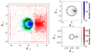 |
Fig. 7 OT Pm = 1 run near dissipation peak (at time t = 1/3tturnover). Hodogram in which the pre-shock magnetic field is normalised and rotated such that |

 |
Fig. 8 ABC Pm = 1 run near dissipation peak (at time t = 1/3tturnover). The left plot is identical to the one presented in Fig. 7. Top right plot shows the number of dots histogram for Parker sheets. Bottom right is for rotational discontinuities. |
3.3.2 Velocity Estimates
The velocity regimes pre- and post-discontinuity completely characterise discontinuity types. However, to estimate them, we must first determine the rest frame of the discontinuity with appropriate accuracy. We compare three independent methods to derive it. The first is mass flux conservation; here, to establish the stationary frame in the SHOCK_FIND algorithm, Lehmann et al. (2016) derived the following from Eq. (24):
 (33)
(33)
where uref is the travelling velocity of the discontinuity in the frame of the computing domain. We note that when the density contrast is weak, the denominator goes to zero, making this estimate prone to large errors.
The second is the most conservative frame. We used all the other conservation relations. We first introduced the travelling velocity uref with the frame change  . We then considered the sum of the squared norms of the left hand sides of Eqs. (25), (26), and (27). When uref is indeed the velocity of the discontinuity relative to the gas, this sum should be zero, because all the conservation relations will be verified. We therefore estimate uref as the velocity that minimises the sum. We note that we drop mass conservation (24) from the sum, because of a mass leak through the working surface of the discontinuities that makes it less accurate. This method is inspired by a more general technique described in Lesaffre et al. (2004) to compute the local stationary frame in multi-fluid 1D simulations.
The last is the stationary wave frame. We used the propagation speed of the most representative wave given by the gradient decomposition at the dissipation peak (see Sect. 2.4). Decomposition in slow and fast waves are always pure right- or left-travelling waves. We then simply chose the velocity at the dissipation peak corresponding to this wave. On the other hand, for intermediate waves, they are often right going on one side and left going for the other. In this case, we take the average velocity weighted by the strength of the corresponding right- and left-going wave (the two averaged velocities usually turn out to both be small).
In Fig. 9, we compare the fluid velocity entering in the discontinuity by the pre-shock side ( ) in the frame established with these three methods. In the top plot, we notice that the mass flux conservation method is inconsistent with the stationary wave frame method for rotational discontinuities and Parker sheets, and to a lesser extent for fast shocks. For Alfvén discontinuities, this is expected because of the weak density contrast, which blows up the denominator in the mass flux conservation estimate. For shocks, the inaccuracy incurred by the mass flux conservation could be due to the difficulty in assessing accurate mass conservation compared to other quantities, as noted in Appendix B. However, it is more likely due to a genuine mass flow that occurs in the dissipating layer of the discontinuity, transversely to the propagation direction. Figure 10 illustrates this phenomenon clearly; stream lines are converging or diverging in the (r⊥1, r⊥2) plane in the last rows. This was a known phenomenon for Parker sheets, where converging flows orthogonal to the reconnection zones are balanced by diverging flows in the plane of the current sheet. However, that this phenomenon is also present for shocks and rotational discontinuities is a discovery. In the case of shocks, we believe this provides the mechanism that allows the relaxation of the post-shock pressure towards that of the ambient medium. Furthermore, the fact that the SHOCKFIND estimate for shocks is biased towards higher values hints at mass loss in the direction transverse to the working surface (or diverging streamlines, opposite the example case shown in Fig. 10, where it should, however, be noted that the velocities are really small, so that this mass loss is almost insignificant).
The bottom plot of Fig. 9 shows a relatively good agreement between the other two independent methods. However, the stationary wave frame tends to give slightly higher velocities for fast shocks and slightly lower ones for slow shocks. For Alfvén discontinuities, the agreement is optimal, and no bias is observed. We chose to use the stationary wave frame in the following because it gives pre- and post-velocity regimes that are more consistent with the RH nature of the discontinuities, which we now check.
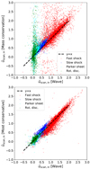 |
Fig. 9 Comparison between different methods to access velocity of gas entering in the discontinuity in its co-moving frame (for the OT simulation at Pm = 1 at time t = tturnover/3). |


3.3.3 Velocity Regimes
With the proper frame set, we can now study the velocity regime transitions. In order to represent upstream and downstream states for all identified scans, we used a scatter plot with a normalisation conditioned by the following regime: super-fast (1), sub-fast/super-Alfvénic (2), sub-Alfvénic/super-slow (3), or sub-slow(4).
 (34)
(34)
 (35)
(35)
 (36)
(36)
 (37)
(37)
where  is the velocity plotted on the diagram and
  is the local positively signed slow, Alfvén/intermediate or fast speed. We note that the usual integers characterising the velocity regimes are in reverse order compared to our renormalised number
  . Figure 11 shows the resulting diagrams. The coloured dashed lines delimit regions specific to the gas velocity regime of a particular discontinuity type (see Sect. 3.3). The columns give pre-discontinuity regimes; from left to right, these are sub-slow, sub-Alfvénic/super-slow, sub-fast/super-Alfvénic, and super-fast. Whereas rows give access to the post-discontinuity velocity regime, with the same sorting from bottom to top.
The diagram in the right of Fig. 11 shows the results for the simulation with OT initial conditions. Because the point density makes distributions difficult to appreciate at the densest regions, we also computed 2D PDFs for shocks, which we used to highlight contours at the value of the median pixel (orange lines) and the third decile one. Scans that are identified as fast shocks are located in the expected region for the most part (identified as 1 → 2 discontinuities). The distribution of scans identified as slow shocks are indeed 3 → 4 discontinuities. However, we note that the slow shocks often have negative velocities out of the shock (not shown). We believe this reflects the fact that the post- shock state is affected by the mass loss in the plane of the shock. The determination of the stationary reference frame by the ‘most conservative’ method gives more positive post-shock velocities (consistently with lower pre-shock velocities as seen in Fig. 9, bottom panel).
The ABC initial conditions case is shown in the left of Fig. 11, where PDF’s contours are now used for Parker sheets and rotational discontinuities. Those two are very peaked at 2 = 3 → 2 = 3, where we expect Alfvén discontinuities in the traditional MHD shock classification (Delmont & Keppens 2011).
For both OT and ABC initial conditions, the distributions of Alfvén discontinuities are stretched in the horizontal and vertical directions. We find in these trailing populations an over-representation of scans in which Bscan ≃ 0 on one side of the discontinuity and not the other. These structures are hence not perfectly plane-parallel, because the magnetic field normal to the discontinuity should be conserved. A nearly zero magnetic field on one side implies that  , and as a result distances between green dashed lines and zeros are artificially expanded by the graph’s normalisation relations (34) to (37). A small error in the determination of the frame velocity and/or the position of the pre- or post-discontinuity positions leads to exaggerated distances between the expected and the actual position of the dots.
The match between our identification criteria and the pre-and post-discontinuity velocity regimes is strongly dependent on the determination of the frame in which the structure is stationary. We checked our three methods, and we found that steady frame velocities obtained from the wave decomposition yield the best consistency between the types and the expected state transition for each type of structure.
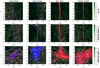 |
Fig. 10 Observation of the local geometry of the velocity and magnetic fields for different types of dissipation structures. First two rows: cuts across the plane rscan−r⊥1 for four examples of structures we identify (for the same four scans as in Fig. 6). Last row: cuts across the plane r⊥1−r⊥2 for the velocity stream lines. Top plots show magnetic field lines, while bottom ones show velocity stream lines. The frame of reference is set to be the stationary wave frame at the centre of these images. The background is a two-channel colour map with red assigned to ohmic dissipation and blue to viscous dissipation. |
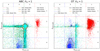 |
Fig. 11 The scatter plot on the left is for ABC, and the one on the right is for OT (Pm =1), both near the dissipation peak. For each scan, we computed pre- and post-shock slow, intermediate, and fast velocities. We compared fluid velocities to these characteristic speeds in the stationary wave frame. We normalised velocities according to the pre- and post-regime following Eqs. (34) to (37). X-axis is the pre-shock regime and Y-axis the post-shock regime. Thus, each kind of discontinuity, in the classical MHD discontinuity classification, belongs to one box. Isocontours in solid and dashed lines were computed for the two most represented kinds of profile. The zones inside the contours delineate the densest area comprising, respectively, 70% (black) and 50% (orange) of the dots. |
4 Results
In this section, we use our identification algorithm to extract statistical results from our simulation set. We study the impact of some of our input parameters on dissipation structures. Our set is composed of simulations with different magnetic Prandtl numbers (Pm) and two different velocity field and magnetic field configurations (see Table 1).
4.1 Impact of Initial Conditions
We consider here the effect of the initial conditions of the simulations on the nature of the structures formed. Figure 12 shows distributions of the identification scans as a function of the mean dissipation rate in the volume probed by each scan, and Table 2 summarises these results averaged over all scans. The time step chosen for the two graphs on the left side of this figure (as well as for the left side of Table 2) is 1/3 of the initial turnover time, shortly after the dissipation peak, when the first and most intense dissipation structures form. The time step chosen for the right hand sides of Fig. 12 and Table 2 is after one turnover.
As described in Sect. 2.1, we used two types of initial flows: ABC and OT. The main difference between these two flows resides in their magnetic and cross helicities (see Sect. 2.1.2). This initially yields very different types of structures. Early time OT is dominated by shocks (mainly fast shocks), while ABC is dominated by Alfvén discontinuities (rotational discontinuities and Parker sheets). After one turnover time, the impact of the initial conditions on the formation of the dissipation structures seems to be erased. The main dissipation mechanism is then through rotational discontinuities and Parker sheets for both ABC and OT.
Interestingly, for both types of initial conditions, at early and late times, the distribution of physical natures of scans does not seem to depend on their level of dissipation. Intense dissipative scans and weak scans have about the same proportions of each nature.
Table 2 also shows the amount of unidentified and misidentified scans. Between 58% and 78% of intense dissipation is identified by our technique, with a greater success rate for ABC than OT. Early time structures are also better identified than later times.
Identification fractions within our scans in number (top) and weighted by dissipation (bottom) for several snapshots and initial conditions in Pm = 1 simulations.
4.2 Impact of the Prandtl Number
One critical parameter of dissipation is the magnetic Prandtl number, Pm = v/η, which is the ratio of kinematic viscosity v to magnetic diffusivity η (see e.g. Brandenburg & Rempel 2019). We performed our dissipation structure analysis on simulations with a range of magnetic Prandtl numbers, from Pm = 1 to Pm = 16 (see Table 1). As dicussed in Appendix B, the intrinsic numerical dissipation from the scheme causes the effective Prandtl number to be slightly different from the input one. Thanks to semi-analytical solutions (computed in Appendix A), we probed the effective Prandtl number of our scheme in 1D MHD shocks. Figure B.4 shows that for moderate velocity shocks (or u0 ≤ 1) our scheme is already converged, while the highest shock velocities we ñnd in simulations are at u0 ≃5. We thus remain confident that the effective Prandtl number in our simulations is overall close to the input one, at least as regards shocks.
Figure 13 shows OT and ABC identification distributions for input Ƥm = 1, 4, 16. The magnetic Prandtl does not seem to have any impact on the distribution of structures. The only noticeable difference is a slight increase in the number of rotational discontinuities at the expense of Parker sheets for ABC initial conditions.
It was shown by Brandenburg & Rempel (2019) that an increase in Ƥm causes an increase in 〈єυ〉/〈єη〉, a result that we confirm and detail here. If there is no statistical difference in high dissipation structure distributions, it must be differences in the internal structure of the dissipation layers that lead to differences in dissipation rates. In Fig. 14, we show scatter plots of viscous versus ohmic dissipation rates, where each dot marker expresses the mean of the corresponding dissipation rate within each scan. At Ƥm = 1, it is clear that rotational discontinuities and Parker sheets are dominated by magnetic energy dissipation. Fast shocks are an intermediate case, with a more balanced share between ohmic and viscous dissipation rates. Slow shocks are dominated by viscous dissipation. Each type of structure is more or less characterised by a given slope in these graphs (i.e. the ratio 〈εv〉scan/〈єη〉scan is within a more or less well-defined sector for each type of structure, regardless of initial conditions OT or ABC). In particular for shocks (both slow and fast), when Ƥm varies, this ratio simply scales as Ƥm. The behaviour of dissipation within fast shock scans follows the rule 〈εv〉scan/〈єη〉scan ∝ Ƥm This scaling is less clear lor the other types of structures: Alfvén discontinuities experience a wider range of ratios at fixed Ƥm which makes it less easy to assess if such a scaling is present (in fact, the envelope of green and cyan points suggests a different scaling, closer to  ). Provided the global dissipation is reflected by intense events, this could explain why the global average ratio 〈εv〉/〈εη〉 is also found to scale approximately as Ƥm in our simulations. We therefore conclude that in our simulations the increase in the viscous over ohmic fraction when Ƥm rises comes not from a difference in the nature of the dissipation structures that form, but from a modification in the way each of these types of structure dissipates internally.
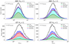 |
Fig. 12 Distribution of different types of structure in terms of the mean scanned dissipation across the discontinuity. The black curve is the total distribution of scans, whereas coloured curves are identified structures’ contributions. The white area corresponds to unknown dissipation scans. Top plots are for ABC initial conditions, while bottom ones are for the OT flow. Distributions on the left are at an early time (≃1/3ttumover). The right panel shows the same distribution at t = ttmmover. |
4.3 Statistics of Entrance Parameters
In this section, we consider values of the state variables at the pre- and post-positions on either side of the discontinuities, and we look for statistical differences between the various natures of discontinuities. The distributions of entrance sonic Mach numbers (see Fig. 15) unsurprisingly show that the entrance velocities are very small for Alfvén discontinuities, moderate for slow shocks, and of the order of the r.m.s. Mach number for fast shocks (but with a widespread distribution). Previous work by Lehmann et al. (2016) showed the distributions of fast and slow shocks display exponential tails at large velocities. We have less statistics, but our data is also consistent with this picture. The bottom row of Fig. 15 displays the distributions for the entrance orthogonal Alfvénic Mach number  . Naturally, it is above 1 for fast shocks, and below 1 for slow shocks. Its distribution for Alfvén discontinuities is more surprising, though, with widespread values ranging up to values above 1, while one would expect it to be close to zero. This comes from the fact that the entrance velocities in these discontinuities are of the order or below the sound speed, but the magnetic field happens to be almost transverse, thus yielding very small values for the intermediate speed
  . Finally, we also looked at the statistical distributions of the density on the pre-discontinuity side and found these distributions were independent of the nature of the discontinuity considered.
The environment of each discontinuity is defined by seven state variables on either side (pre- and post-) of the discontinuity, giving a total of 14 independent state variables. We can reduce this number by using the seven conservation relations (mass, momentum and magnetic field, and 7 independent variables), a normalisation by the pre-discontinuity density (1 variable), a rotation of the transverse axes to cancel one component of the pre-discontinuity magnetic field (1 variable), as well as a transverse boost of the frame to cancel the transverse velocity components’ pre-discontinuity (2 variables). The environment can thus be fully characterised by a remainder of three independent variables, which can all be considered on the pre-discontinuity side.
For these three independent ‘entrance parameters’, we chose the normal p1 and transverse p2 magnetic pressures as well as the difference р3 between the ram pressure and the normal magnetic pressure (all are normalised by the thermal pressure p = ρc2). This choice makes it easy to predict where each discontinuity should lie in the 3D parameter space, according to the sign of p3. Negative is for slow shocks, zero for Alfvén discontinuities, and positive for fast shocks, while p1 and p2 could be arbitrary positive numbers.
Figure 16 displays two projections of this 3D space onto the planes (pз,p1) and (р3,р2)- In this parameter space, the only forbidden region is set by the positivity of the ram pressure 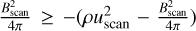 , which translates as p1 ≥ −р3. However, we find it is not the only region that is devoid of points: the entrance parameters of our structures do not fully explore the available parameter space. In fact, tight correlations for fast shocks are visible in the right hand panel of Fig. 16 (where
  and similarly for the slow shocks in the left hand panel (where
  ). It also appears that rotational discontinuities and Parker sheets are preferably parallel to the magnetic field (Bscan≪ B⊥). The latter two discontinuity types are not distinguishable in this parameter’s space, as we only considered the pre- and post-discontinuity states here without taking into account the internal structure.
These statistical constraints on the three entrance parameters of the dissipation structures reduce the number of independent parameters to two. Understanding the origin of these correlations in MHD turbulence will be the subject of future work.
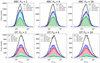 |
Fig. 13 Dissipation structures distributions for our two initial conditions with varying magnetic Prandtl number from Pm = 1 on the left to Pm = 16 on the right. The time step shown here is at an early time, near the dissipation peak. |
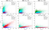 |
Fig. 14 Distributions of ohmic and viscous dissipations averaged within each scan, for the ABC simulation above and OT below, according to the different identifications and for the values of the magnetic Prandtl ranging from Ƥm = 1 on the left to Ƥm = 16 on the right. |
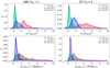 |
Fig. 15 PDFs of entrance sonic (top row) and Alfvénic (bottom row) Mach numbers in the Ƥm = 1 ABC (left) and OT (right) simulations at time t = tturnover/3. |
4.4 Transverse velocity differences
Molecular line observations probe the radial velocities across the plane of sky, while we have access to the full 3D geometry of the intense dissipation regions in our simulations. When projected on the plane of sky, an intense dissipation sheet yields a salient, filament-like feature on observable maps where the plane of the sheet is orthogonal to the plane of sky, id est where column-density is greatly enhanced through a caustic-like effect. In Fig. 17, we hence display the velocity difference statistics projected on the two transverse directions,  and
and  , as a proxy to what an observer would measure for the velocity difference across the projected ridge of an intense dissipation sheet, in the two cases where the line of sight is along
  or
or  . As expected due to rotation symmetry, rotational discontinuities have no noticeable difference depending on the direction, while fast and slow shocks are co-planar; hence, the difference is greater in the direction of
  than in the direction of
  . What is more surprising, though, is the fact that Parker sheets follow the same trend as rotational discontinuities; this is an indication that there is more continuity between the rotational discontinuity and Parker sheet classes than our arbitrary division between the two would suggest. An interesting feature we also observe is the bimodality of the slow shocks compared to the fast shocks, which is linked to the fact that
  needs to be greater than the typical velocity to yield a slow shock.
We retained the sign of the velocity differences, although they technically cannot be probed by observations, due to the unknown projection angle. In the OT case, the positive and negative velocity differences for slow and fast shocks along  have markedly different statistics. This is due to the relative orientation between the fluid velocity and the magnetic field direction along the scanning vector. When they have the same orientation (i.e. Bscan = Bn > 0), transverse velocity differences have the same sign as transverse magnetic field differences (see Eq. (29)): in this case, fast and slow shocks have, respectively, positive and negative velocity differences. For the OT initial conditions, the positive cross-helicity results from a mean positive alignment between velocity and magnetic fields, hence a more likely positive velocity difference for fast shocks, or negative for slow shocks. For the ABC initial conditions, the mean cross-helicity is zero, which yields symmetric statistics.
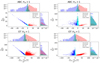 |
Fig. 16 Entrance (pre-discontinuity) parameters for each scan we identify at time t = tturnover/3. The position of the pre-discontinuity is defined in Sect. 3.3 (as three times the dissipation length ℓɛ before the dissipation peak). Top plots are for ABC initial conditions and bottom plots are for OT ones. The x-axis is the difference between ram and magnetic normal pressures. In left plots, the y-axis represents the magnetic pressure in the scan direction, and in the right ones it represents the transverse magnetic pressure. All quantities are normalised by the thermal pressure (p = pc2). Integrated PDFs are given on each side of the panels. |
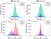 |
Fig. 17 Transverse velocity differences in the two directions |


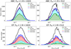 |
Fig. 18 Nature-by-nature distributions of dissipation flux per scan in our Ƥm = 1, 10243 simulations (leftpanels) and in our 5123 simulations (right) at t = 1/3ttumover. |
5 Discussion
5.1 Resolution Study
We performed simulations at half the resolution (5123 pixels) in order to check the stability of our results, we note that the dimensions of our scanning cylinders are defined with respect to the pixel size, with three pixels in lateral radius and a 6 ℓɛ scanning length centred on the detected local maxima of dissipation. The appropriate quantity to consider is hence the average energy dissipation rate per unit surface or the energy flux through the surface of the discontinuity.
In Fig. 18, we consider the statistics of these dissipation fluxes nature by nature for two corresponding runs at 5123 and 10243. They are seen to match perfectly, except for statistical noise, which disrupts the lower resolution results. Indeed, we identify approximately four times fewer scans at low resolution, which is another indication that our dissipation structures are mainly sheets.
We also find that for both N = 512 and N = 1024, ℓɛ is of the order of 1.5 pixels. This is consistent with our findings on ID shocks in Appendix В that a two times lower resolution would yield an energy deposit twice as wide spread in the scanning direction, while keeping its integrated value constant (thanks to our method to recover numerical dissipation). It is also a hint that the same behaviour holds for Alfvénic discontinuities, which was not obvious.
Finally, this is another indication that large-scale dynamics set the environmental characteristics of the discontinuities (the values of the state variables of the gas on either side of them), while the microphysics (physical and numerical dissipation) control the internal profiles of these discontinuities. The first evidence of this was uncovered with our Prandtl number study in Sect. 4.2.
5.2 Towards Global Dissipation Fractions
In this paper (Sect. 2.1.2, for example), we discuss the relative distributions within our scans. However, it is unfortunately difficult to relate it to the global dissipation in the computational domain, because the scans focus on the most intense events. Nevertheless, in Sect. 3.1 we show that strong dissipative pixels considered in this study (>4σ) represent a large fraction (≃25% for ABC near the dissipation peak and ≃30% for OT) of the global dissipation rate of the simulation time step. However, the dissipation rate only exceeds this threshold near the peak of each scan, so the dissipation in a given scan also accounts for some dissipation below that threshold. Hence, the dissipation within our scans must amount to more than these global fractions of dissipation. Furthermore, if we had chosen a lower threshold to identify structures, we would have detected weaker scans closer to the lateral edges of the dissipation structures. Since the proportions in physical natures do not appear to depend much on the strength of the scan, we might expect to find the same proportions in these weaker scans. As a result, the fractions we currently measure might apply to a more significant fraction of the global dissipation, although it is difficult to ascertain it (overlap between scans of neighbouring structures and lack of planarity for some of the weaker scans might moderate the above arguments). In particular, we are not able to assess whether there is a diffuse component of dissipation outside the intense dissipative regions.
5.3 Pixel-by-Pixel Distribution
Our method identifies a large majority of the scans we probed in each simulation and time steps studied. The criteria for the identification of the scans are very strict, with the aim of discovering the structures’ basis causing the dissipation in the isothermal compressible MHD regime. Although restricted to the purest structures, we identify a significant fraction of the total dissipation of the simulations. In Sect. 5.2, we mention the difficulty of relating total dissipation rates to the scan distribution. Here, we attempt to link the distributions of scans to the distribution of the pixels above a given threshold. To partly remedy overlapping problems that might occur between scans, we flagged cells above a given threshold of the simulation according to the first identification that contain them. The resulting dissipation rate identification is shown in the top plots of Fig. 19.
The black line shows the fraction of dissipation captured by the threshold four standard deviations over the mean. The colours below show the fraction of each pixels above this threshold identified as each of the four main natures we find in our scans (the white space combines pixels that were never flagged because they always fall in unidentified or unknown scans). This time evolution graph clearly shows how the distributions differ at early times for our two different initial conditions, and how they stabilise after little bit less than one turnover time. This confirms the result that we found for scan distributions and state in Sect. 4.1.
5.4 Connectedness
Furthermore, if we consider only the well-identified scans, we observe that about 70% of the related connected structures are identified by a single type of scan and 80% have more than 75% of their scans identified by the same nature (see Fig. 20). We can therefore consider propagating the dominant type of a connected structure to the remainder of its cells. This allows us to avoid the edge effects of structures and increases the identified dissipation fraction. The result is shown in the bottom plots of Fig. 19. This graph tells us, first of all, that the fully unidentified connected structures, although representing a significant fraction of the studied structures in number, participate very little in the total dissipation of the cube. These are small fragmented events, which also comprise the short filament-like structures seen in Fig. 3. Second, we notice that the unidentified scans often belong to structures dominated by rotational discontinuities, except for the OT simulations at an early time, when they are sometimes part of fast shocks (see Fig. 20). For ABC runs, until about 0.7 turnover times, the dissipation generated by the Parker sheets decreases slightly to the benefit of that produced by the rotational discontinuities (bottom right panel of Fig. 19). This implies that despite the uniqueness of the identifications within a related structure, a significant fraction of the Parker sheets are found within structures formed by rotational discontinuities, which relates to our previous remarks on the continuity between Parker sheets and rotational discontinuities; our divide between the two is rather arbitrary, and these connected structures could probably be gathered into a single Alfénic discontinuity class.
We also tried to decrease the detection threshold of the dissipation structures to  to increase the fraction of the total identified dissipation. In this case, the identification rate decreases only by a few percent compared to a threshold of
  . The contribution of the different natures to the overall dissipation remains similar, and the fraction of dissipation above the threshold identified by the scans increases by about 10% overall.
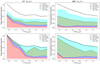 |
Fig. 19 Contribution of dissipative structures and their different natures to global dissipation. Top plots: fraction of the total dissipation high dissipation structure contribute to (black line) and the contribution of cells that belong to a scan that is identified (coloured areas) for OT and ABC initial conditions simulations. Bottom plots: we use the most represented identification in each structure and attribute the total dissipation rate of the structure to this kind. This method is supported by the fact that we find connected structures to be mainly made of one kind of discontinuity. |
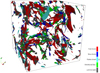 |
Fig. 20 High-dissipation structures extracted from an OT initial conditions simulation at Ƥm= 1. The time step of this output is t ≃ 1 /3ttumover. |
5.5 Unknown Identifications
By using two sets of criteria that are rather independent of each other, we biased our identifications towards more false negatives and fewer false positives. Thus, there remain many misidentified scans, because they either do not fit any of our heuristic criteria (unidentified scans) or because the two sets of criteria do not match (misidentified scans). We outline some of the reasons why our identification criteria might miss a significant fraction of the scans.
The main culprits are ‘edge’ scans. These are scans at the periphery of structures where the main direction of the gradient is less well defined, and therefore the scanning direction is less relevant. For instance, the scanning direction is irrelevant in the case of the small, filament-like structures observed in Figs. 3 and 20, where scans probably fall at least in the misidenditified category. Also, when two structures are too close to each other, the heuristic part of the identification is confused, because bumps or jumps are less well defined. We note that the wave decomposition suffers less from adjacent structures, because it is sensitive only at the cell scale. Some of the unidentifications could also be due to the presence of intermediate shocks (see Sect. 5.6 below) but we consider that they probably account for only a small fraction.
Given the strong correlation between our two sets of identification criteria (heuristic and ideal waves), one could suggest using only ideal wave decomposition to greatly increase the identification rate. We would thus reach 100% of identification, but our results would then be subject to caution and biased towards false positives. One should restrict this wave-only decomposition to the most planar cells where the gradient approach makes sense. Also, the identification would then rely on the velocity regimes, which we have shown can be subject to caution depending on the method used to estimate the travelling speed of the discontinuities.
5.6 Intermediate Shocks
If intermediate shocks are present in our simulations, our heuristic criteria would voluntarily miss them, and they would fall in the unidentified category. These shocks have either a density or a pressure jump, but they often display a magnetic field trough. We chose not to add this criterion here because we would not have had an independent criterion for gradients to solidify this heuristic one. This might be a reason why we achieve less identification in the OT case at early times, which seems more prone to generating shocks. We in fact attempted to target intermediate shocks and have found some convincing cases. However, the uncertainty on our estimate for the steady state velocity of these discontinuities makes it difficult to validate the speed regimes of these shocks on a statistically significant population. We hence decided to postpone our investigation on these shocks. In any case, the fraction of unidentification that we publish here puts an upper limit on the fraction of intermediate shocks.
5.7 Driven Versus Decaying Turbulence
Some astrophysical situations (a solar coronal ejection, a supernova, or a runaway star encountering a cloud, for example) can locally inject mechanical energy in a short amount of time. In these events, well defined initial conditions that can suddenly be imposed and will later develop into turbulence. In these contexts, decaying turbulence is probably a sensible approach. However, one can question the applicability of decaying turbulence in many other realistic astrophysical situations. First, turbulence being ubiquitous, it is very unlikely that an initial set-up would be entirely devoid of turbulent perturbations at the onset. Also, the fast decay of turbulence led Stone et al. (1998) amongst other authors to advocate the necessity of persistent driving at the scales relevant for the interstellar clouds. Our experiments have shown that initial conditions can imprint significant changes in the early phases of the development of turbulence; similarly, we expect that a given forcing may impact the resulting turbulent cascade at least to some degree, and it will do so at all times. One should therefore be careful to properly characterise the properties of the forcing (such as helicity injection) used in the experiments of driven turbulence.
In particular, a lot of attention has been devoted to the importance of solenoidal versus compressible forcing (Federrath et al. 2010). This has led to techniques for observationally probing the degree of compressibility of the gas; some regions of the ISM near the galactic centre were found to be dominated by solenoidal driving (Federrath et al. 2016), while others associated with stellar feedback were found to be more compressively driven (Menon et al. 2021). Intermediate situations were also witnessed in Orion B (see Orkisz et al. 2017, for example). These considerations are important, as the nature of star formation is believed to be strongly influenced by the driving of the turbulence (Federrath & Klessen 2012). In the present study, we did not attempt to check the influence of compressible versus solenoidal initial velocity fields (our initial velocity fields are divergence free), but one can imagine that initially more weight would be given to shocks had we started with velocities including a compressive component. We still believe though that the tendency to evolve towards incompressible structures would persist (imagine starting the origin of times after a fraction of the turnover time: this might be an illustration of what could happen if we started the simulation with compressible initial conditions). Finally, an intermediate solution would be to start decaying turbulence with a snapshot of fully established driven turbulence, or to imprint synthetic models of turbulence, such as those designed by Durrive et al. (2020), on the initial conditions.
6 Conclusions and Prospects
The aim of the present study is to systematically characterise the physical nature of intense extrema of dissipation in MHD simulations of turbulence. We developed a technique to locally recover the total dissipation including the numerical losses. We tested the classic rule of thumb that grid-based simulations need twice the resolution of similar spectral schemes; in this case, we find that numerical dissipation is indeed below half of the total, but dissipative fronts are widened by a factor of about three. Since obtaining the expected thickness would require an extra factor of ten in resolution, we feel the current usage provides a good compromise.
We devised a way to characterise the geometry and the physical nature of local intense variations of the state variables of the gas. We find the non-linear waves associated with these large gradients and disclose their Rankine–Hugoniot category. We show that at the dissipation peak, the fully dissipative gradients must be close to an ideal MHD wave gradient. We observe that the nature of this gradient is surprisingly consistent throughout the profile of the dissipation structure. For example, fast shocks are composed of essentially fast wave gradients, and we confirmed it with the 1D semi-analytical models of isothermal shocks of Appendix A. We used this property to our advantage and we designed a method to classify the dissipation structures into fast shocks, slow shocks, Parker sheets, and rotational discontinuities. We successfully identified a large majority of the intense dissipation, which allows us to draw statistical conclusions.
We show that initial conditions can strongly affect the nature of the dissipation structures at early times. However, early signatures of the initial conditions are quickly lost after about one turnover time. At this point, dissipation becomes dominated by weakly compressive structures (Alfvén discontinuities rather than shocks). This may be due to the sonic Mach number having decreased closer to one at this point. We aim to investigate higher Mach numbers and more compressive initial conditions in the future.
Despite the complexity of the magnetised 3D flows we investigated in this study, the strongest dissipation structures are locally planar and steady and can be assimilated to Rankine– Hugoniot discontinuities. We noted unexpected correlations between the entrance parameters of these discontinuities (which can be reduced to a 2-parameter family); further work is needed to explain how these correlations arise in a turbulent medium.
We compared three methods to measure the travelling speed of these non-linear waves and checked that the resulting velocity regimes are compatible with our identifications. The difficulty in accurately measuring the travelling speed makes it impossible to assess the statistics of the elusive intermediate shocks, although we report we could find clear examples of them (not shown in this paper).
The access to an accurate travelling speed will facilitate the follow-up of structures in time, which will help discover if the statistical changes with respect to time are due to collisions (or breading) between structures, birth or death of given structures, possible changes in nature of a given structure in time or to the development of substructures and instabilities within a structure.
We do not find strong evidence for the slow shocks being more subject to corrugation instability as originally found by Park & Ryu (2019). In general, connected structures appear equally fragmented regardless of their various natures (see Fig. 20), but a more quantitative study might conclude otherwise. It seems to us that Alfvénic discontinuities are often found in parallel sub-layered systems, while fast shocks often occur in isolation, but again a quantitative analysis might conclude otherwise.
One may challenge the applicability of such simplified isothermal MHD simulations to a medium as complex as the interstellar medium. However, the present study hints that, to some extent, the details of the microphysics matter only within the internal structure of discontinuities. For example, the statistics of the entrance parameters do not change when Ƥm is varied. This is reminiscent of the study by Brandenburg (2014), which suggested that variations with Ƥm were controlled by the individual 1D structure of the shocks, and it is also echoed in the review of reconnection by Zweibel & Yamada (2016), which focuses on the respective roles of global and local processes. If this holds, one could imagine post-processing the statistics from 3D simulations with more detailed 1D models including non-equilibrium chemistry, such as the Paris-Durham shock models (Flower et al. 1985; Flower & Pineau des Forêts 2015), as was demonstrated in Lesaffre et al. (2020) for 2D unmagnetised turbulence.
The ultimate objective is to estimate the turbulent dissipation rate in diffuse matter and its characteristics in the broad perspective of unravelling molecular cloud growth and star formation (e.g. Hennebelle & Falgarone 2012). The fall-off (or the absence of fall-off at small scales) of power spectra of a variety of tracers of diffuse interstellar matter (e.g. Miville-Deschênes et al. 2016) is a key piece of information to be combined with the kinetic information provided by high-spectral-resolution observations of either atomic gas (e.g. Reach & Heiles 2021) or molecular lines (Hily-Blant et al. 2008; Falgarone et al. 2009). This latter route is of course challenging because it requires the modelling of non-equilibrium chemistry driven by dissipation bursts.
Conversely, our multi-dimensional simulations suggest improvements to 1D traditional models. Although the structures we find are mostly plane-parallel, we find that the main deviation from 1D profiles is sideways mass loss into the dissipative sheet. In the future, we can imagine refining 1D models by including such mass loss, as did Parker in his fiducial Parker-sheet model, for example (Parker 1963).
Finally, we believe that the tools we put forward in this paper will give more ground to the view of developed turbulence being a statistical collection of coherent structures. For example, a series of works (e.g. Zhdankin et al. 2013, 2014, 2015, Zhdankin et al. 2016) on the dissipation structures in reduced MHDs has led to new insights on the analytics of intermittency and turbulent dynamics by Mallet & Schekochihin (2017). Density statistics deviations from log-normal were explained by an appropriate collection of shocks in Robertson & Goldreich (2018). Recent development in the theory of anisotropic compressible MHD turbulence use to their advantage the statistics of shocks to interpret the probability density function of the density (Beattie et al. 2021). In the meantime, Cluster satellite observations (Perrone et al. 2016, 2017) have witnessed the signatures of both Alfvén and compressive coherent structures in the fast and slow components of the solar wind. Recent developments in solar wind observations may soon be able to constrain the statistics of the various individual types of dissipation structures (Bruno & Carbone 2013).
Acknowledgements
We thank our referee, Christoph Federrath, for his constructive comments which helped us improve the quality and scope of the manuscript. The research leading to these results has received fundings from the European Research Council, under the European Community’s Seventh framework Programme, through the Advanced Grant MIST (FP7/2017–2022, No. 742719). Computations were performed on the cluster Totoro funded by the MIST ERC and hosted by the computing center mesoPSL. We thank S. Fromang who provided us with his version of DUMSES. We thank Ben Snow for enlightnening discussions on intermediate shocks and Erwan Allys on dissipation scalings with Ƥm for each type of structure. The idea of gradient decomposition into linear waves is our generalisation to 3D MHD of a method communicated to us by Johann Carroll-Nellenback who previously used it on Astrobear 1D hydrodynamical simulations to detect shocks and contact discontinuities.
Appendix A Steady-State 1D MHD Shocks
Here, we consider the internal structure of a steady-state isothermal planar MHD shock. We can always operate a Galilean transformation to place ourselves in the frame moving along with the shock, so that the pre-shock velocity is in the normal direction to the working surface, which we define as the first space coordinate x. In addition, we can rotate this frame along the normal so that the second space coordinate y is along the pre-shock transverse magnetic field, and so both third components z of the magnetic field and the velocity are zero along the whole shock (thanks to the co-planarity property within shocks; this would not be the case in a rotational discontinuity).
We write u and υ for both the first and second coordinates of the velocity in this frame, and similarly we write Bx and By the coordinates of the magnetic field (orthogonal to the working surface and transverse). We finally write ρ as the mass density and x as the first space coordinate.
With these notations, the isothermal conservation of mass, momentum, and magnetic field become:
 (A.1)
(A.1)
![Mathematical equation: $0 = {\partial _x}\left[ {\rho {u^2} + \rho {c^2} + {1 \over {8\pi }}B_y^2 + {4 \over 3}\mu {\partial _x}u} \right],$](/articles/aa/full_html/2022/08/aa42531-21/aa42531-21-eq148.png) (A.2)
(A.2)
![Mathematical equation: $0 = {\partial _x}\left[ {\rho uv + {1 \over {4\pi }}{B_y}{B_x} + \mu {\partial _x}v} \right],$](/articles/aa/full_html/2022/08/aa42531-21/aa42531-21-eq149.png) (A.3)
(A.3)
 (A.4)
(A.4)
![Mathematical equation: $0 = {\partial _x}\left[ {u{B_y} - v{B_x} + \eta {\partial _x}B} \right],$](/articles/aa/full_html/2022/08/aa42531-21/aa42531-21-eq151.png) (A.5)
(A.5)
where we introduced the dynamical viscosity μ = ρv and the resistivity η coefficients as well as the isothermal sound speed c. We now affect subscripts 0 to the pre-shock quantities (except for the orthogonal magnetic field Bx, which is constant throughout the shock). The mass conservation becomes ρu = ρ0u0. We define the quantity  , which has the dimension of a velocity, and, similarly, the constant Alfvén speed
  , to arrive at the following system of ordinary differential equations:
 (A.6)
(A.6)
 (A.7)
(A.7)
 (A.8)
(A.8)
to compute the internal structure of isothermal MHD shocks.
The isothermal dynamical coefficient μ is a constant, but in the current application we used a constant viscous coefficient v, so that μ = vρ0u0/u. The typical viscous length scale of our simulated shocks is hence v/u0. One can further simplify the above system by using the non-dimensional quantitites  , and Ƥm = v/η:
 (A.9)
(A.9)
 (A.10)
![Mathematical equation: ${\partial _{\tilde x}}\tilde a = {{\cal P}_{\rm{m}}}\left[ {{\cal M}_a^{ - 2}\left( {\tilde a - 1} \right){{{a_x}} \over {{a_0}}} - \tilde v} \right],$](/articles/aa/full_html/2022/08/aa42531-21/aa42531-21-eq160.png) (A.11)
(A.11)
which shows that the intrinsinc structure of our shocks depends essentially on three non-dimensional parameters in the pre-shock: the sonic Mach number  , the transverse Alfvénic Mach number
  , and the tangent of the angle of the magnetic field with respect to the shock working surface ax/a0.
This system of ordinary differential equations (ODEs) can be integrated numerically between the pre-shock (at  and
and  ) and the post-shock. The stability analysis towards increasing
  of these two steady points yields three growing or decaying eigenvectors. We find fast shocks usually have three unstable eigenvectors at the pre-shock, while they have three stable eigenvectors at the post-shock; one can simply integrate the system of ODEs from the post-shock to the pre-shock from a small perturbation of the post-shock opposite the most stable eigenvector (which is the most unstable one in the direction of decreasing
  ). We find slow shocks usually have two unstable eigenvectors at the pre-shock, while they have two stable eigenvectors at the post-shock; the solution leaves the pre-shock from its unstable plane and reaches the post-shock in a stable plane. To find the solution, we used a boundary value solver with a request to be on both these planes at a small given distance from the two corresponding end points. We used the resulting solutions as reference models to benchmark the results of the dedicated experiments, which we describe in the section below.
Appendix B Numerical Dissipation in Godunov Methods
We report here on the method we used to recover the amount of numerical dissipation present in our compressible simulations and how we validated it using the above isothermal MHD shocks. In our compressible simulations, we adopted twice the resolution of corresponding incompressible runs that we performed with pseudo-spectral methods in Momferratos et al. (2014): 1024 versus 512, for the same dissipation coefficients (viscosity and resistivity). Indeed, there is a common belief that grid-based methods need twice as many elements to obtain a resolving power equivalent to Fourier elements. However, we see that even in this case, the numerical scheme still affects the dissipation in the code considerably.
Appendix B.1 Experimental Set-Up
In order to check and control the dissipation in our configuration, we ran 1D planar isothermal magnetised shocks with various resolutions and compared them to the solutions devised in the previous section. To set up the computational experiments of this section, we first computed the Rankine-Hugoniot conditions for a magnetised shock in the shock frame, and we initially set up the pre-shock and post-shock conditions in two halves of the computational box, with the jump in the middle. The outer box boundaries are inflow and outflow conditions on each side of the pre-shock and post-shock material, respectively. As the computation proceeds, the initial discontinuity smears out due to both numerical and physical dissipation, but the discontinuity does not move in space thanks to the chosen set-up. A steady state is quickly reached, which we compare to semi-analytical solutions of the steady state as described in the previous sub-section.
Appendix B.2 Viscous Spread in the Shock
Shocks have a viscous spread of the order of λv = v/u0 (see section A). Our 3D simulations of decaying turbulence with 10243 pixels have a box length of Lbox = 2π and viscosity of v = 0.7 × 10⁻³ , and so the pixel size is nearly nine times bigger than the viscous length for a u0 = 1 shock; the viscous and resistive spread throughout these shocks is realised essentially by the grid. In Lesaffre et al. (2020), we showed that the number of zones necessary to fully resolve the viscous spread of isothermal shocks is at least of the order of the Reynolds number L.u0/v ≃ 9000, which is far above what we can afford for a 3D computation.
Appendix B.3 Dissipation Natures
There are several sources of dissipation in our simulations: viscous and ohmic dissipation due to the physical terms we have introduced in DUMSES, and numerical dissipation intrinsic to the scheme. Our main purpose is to locally recover the total amount of dissipation εtot produced by both the scheme and the physical dissipation terms. We designed several methods to retrieve εtot by considering variants of the energy conservation equation.
Appendix B.4 Method 1
We consider the evolution equation of kinetic and magnetic energy:
 (B.1)
(B.1)
where εtot is the total irreversible heating and where the flux ℱ1 reads
 (B.2)
(B.2)
We computed the left hand side of Equation (B.1) along a replay of a time step of the simulation, using the flux estimates of each dissipative half-step for the resistive and viscous contributions to ℱ1 and using a Lax-Friedrichs estimate for its non-dissipative part (evaluated within the Godunov step). We estimated u.∇(p) at the middle of the time step thanks to the same total variation diminishing (TVD) slopes used in the Godunov step. Finally, we recovered εtot simply by taking the opposite of the left hand side.
Appendix B.5 Method 2
 (B.3)
(B.3)
where
 (B.4)
(B.4)
We computed the flux as in method 1 (the additional contribution is computed in the Godunov step using a Lax-Friedrichs estimate). This method has the advantage that we recover exactly the total heating through the computational domain when we average the local resulting heating.
Appendix B.6 Method 3
 (B.5)
(B.5)
where
 (B.6)
(B.6)
We evaluated −p∇.u as u.∇(p) in method 1 and retrieved εtot as in the previous two methods.
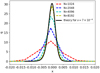 |
Fig. B.1 Dimensionless dissipation in a steady-state fast shock (with dimensionless parameters |

Appendix B.7 Benchmark and Comparison
We checked that the implementations of the three methods on our shock experiments yield the same local total dissipation rate to within less than 1% of the peak dissipation. This gives us confidence in our implementation of the three methods. We also checked on two actual snapshots of our simulations (ABC and OT runs after one turnover) that the statistics of the three methods are nearly identical for the distribution of positive values for the retrieved dissipation εtot. However, method 2 yields significantly fewer pixels with negative values, presumably because this method does not require an estimate for terms such as p∇.u and −u.∇(p), which are not divergences of fluxes. We further note that the means of methods 2 and 3 are really close to one another (less than 0.5% of the standard deviation of εtot), while those of 1 and 2 are a bit further apart (less than 3% of the standard deviation). We therefore adopted method 2 as the best compromise between methods 1, 2, and 3.
Appendix B.8 Numerical Convergence
Figure B.1 shows the irreversible heating rates in non-dimensional units with a close-up of a fast shock front. It illustrates the convergence of the total dissipation rate profile for increasing resolutions. We integrated the total dissipation across the shock and checked it matched the theoretical value obtained by computing the difference of the flux ℱ2 between pre-shock and post-shock values. The integral of the total dissipation rate across the shock is thus always preserved. The effect of the resolution is only to smear out the dissipation profile without changing its total amount.
Figure B.1 is similar to Fig. A2 of Lesaffre et al. (2020), but here we considered it for magnetised isothermal shocks instead of hydrodynamic adiabatic shocks. It demonstrates that the resolution convergence for the heating rate is very slow and fully obtained only for N = 8192 (see the dashed lines approaching the black solid line in Fig. B.1). The situation corresponding to our 3D simulations is the red curve (N = 1024); the viscous heating is largely underestimated and spread out by about a factor of three.
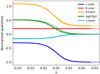 |
Fig. B.2 Comparison of profiles of various state variables of the gas for the same fast shock as Fig. B.1 between the results of our simulation at N = 1024 (dotted lines) and the best-fit model (solid line). Best fit coefficients are v = 2.2 × 10⁻³ and η = 1.7 × 10⁻³ (input coefficients are η = v = 0.7 × 10⁻³). |
We note that for a velocity larger by a factor of two, the analytical solution yields a two times thinner dissipation peak, so the numerical spread would be even larger compared to what it should be. Had we used a constant dynamical viscous coefficient μ, the viscous spread would respond to density in addition to velocity, and the situation would be even worse on the dense side of the shock or for shocks penetrating denser material. Finally, we note that such a slow convergence rate (at most 30% better accuracy for each doubling of the resolution) could lure an unaware numericist into thinking his/her simulations are converged.
Appendix B.9 Dissipative Coefficients’ Fit
We fit viscous isothermal MHD shock models from Appendix A to the velocity and magnetic field profiles, and we recovered best fit values for the viscosity and the resistivity coefficients, which allow us to retrieve the effective viscous and resistive coefficients of our numerical scheme in the case of magnetised shocks. This is a complementary method to that proposed by Lesaffre & Balbus (2007) for non-linear Alfvén waves.
Figure B.2 shows the comparison between the semi-analytical models of the previous section for the best fit η and v and the actual profile for the same shock as in Fig. B.1 and a resolution of N = 1024 pixels. We note that the density is not as accurate as the other variables, and so we discarded it from the fit to retain only the velocity and magnetic field components. This is because the mass flux conservation ρu is estimated at interfaces, and the extrapolation of ρ and u, whereby one increases while the other decreases makes it worse for the product. On the other hand, all other conserved quantities have a product of quantities either both increasing or decreasing, which renders the extrapolation more accurate for the product.
In Fig. B.3, we show an exploration of the effective viscosity thus recovered when varying the resolution. The effective viscosity tends towards the actual input value when the resolution increases, which independantly illustrates the numerical convergence explored in the previous subsection. Because faster shocks have a smaller viscous spread, the effective viscosity is larger for faster shocks, with a required resolution proportional to the entrance velocity of the shock. The type (slow or fast) of the shock does not seem to affect the effective diffusivity of the scheme significantly. At poor resolution, the effective viscosity is inversely proportional to the zone number. Our chosen resolution N = 1024 corresponds to the end of this linear relation between resolution and scheme diffusion; higher resolution would yield a relatively lower increase of accuracy.
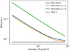 |
Fig. B.3 Comparison between fitted v and input v (dotted black line) for various resolutions and three different shocks. A slow shock |


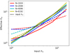 |
Fig. B.4 Comparison between effective Ƥm and input Ƥm (dotted black line) for various resolutions and the two fast shocks of Figure B.3 (solid lines for u0 = 1 and dashed lines for u0 = 4). Ƥm was varied by keeping the value of the resistive coefficient η = 0.7 × 10⁻³ fixed while varying the value of the viscous coefficient accordingly v = ηƤm. |
We also explored the capacity of the scheme to account for various Prandtl numbers Ƥm by increasing the viscous coefficient with respect to the resistive coefficient. Because the scheme increases the diffusivity, the overall span for the Prandtl number is not as wide as for the input physical value. The situation is even worse for the greater velocity shocks, but a resolution of 1024 pixels still allows a comfortable probing range of Ƥm. Slow shocks at Ƥm > 1 are not sensitive to the Prandtl number, and so they could not be used to probe its effective value due to the numerical scheme. This is because when Ƥm > 1 in slow shocks, the magnetic field profiles are dominated by the kinetic-to-magnetic energy transfers as the resistive terms become negligible.
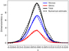 |
Fig. B.5 Our numerical estimation (dashed) of total (black) ohmic (red) and viscous (blue) dissipation in the same fast shock as Fig. B.1 compared to the actual quantities in the best-fit model (solid lines with corresponding colours). We note that the correct share between ohmic and viscous dissipation relies on the effective Ƥm being close to the actual input value of Ƥm, so the method we use is worse for greater velocity shocks. |
Appendix B.10 Ohmic Versus Viscous Dissipation
Although thanks to our method we gained access to the total numerical dissipation, we could not find an accurate way to separate the numerical dissipation of magnetic fields from the numerical dissipation of kinetic energy. In order to compute corrected values for the viscous heating and the ohmic heating, we simply shared the total numerical heating between each of them in proportion to their relative physical values, namely  for viscous dissipation and, conversely for ohmic dissipation,
  . Whenever our estimate for the purely numerical dissipation is negative (i.e. εtot < εv + εη), we simply set
  and
and  . We then computed the viscous and ohmic heatings in the best fit shock model and compared them to the above estimation in Figure B.5.
Appendix B.11 Summary
We controlled the implementation of our dissipation rate recovery method by comparing several variants of it, and we bench-marked them against analytical solutions. We find that we are able to recover the total dissipated energy within a localised shock with very good precision. We used the benchmark models to estimate the diffusivity of the scheme and we find that the effective viscosity and resistivity are both enhanced due to lack of resolution, especially for the large velocity shocks. As a result, the effective Prandtl number is also affected. On the other hand, the slow convergence to the shock solution justifies our use of a moderate resolution associated with this dissipation recovering method. We would not gain much by running our simulations at twice the current resolution, while we would have to increase the resolution more than tenfold to make use of this dissipation recovery method.
Appendix B.12 Prospects
The numerically acute reader will have noted that our method is currently limited to Lax-Friedrichs implementations of the Riemann solver. Other Riemann solvers require us to design a method to incorporate the additional components of the fluxes ℱi. We checked slow and fast shocks, and they seem equally well treated at equivalent velocities. However, we did not check the effective diffusivities in rotational discontinuities (although non-linear Alfvén waves such as those used in Lesaffre & Bal-bus (2007) may provide a good estimate) or Parker sheets (these require at least a 2D treatment).
References
- Appleton, P.N., Guillard, P., Boulanger, F., et al. 2013, ApJ, 777, 66 [NASA ADS] [CrossRef] [Google Scholar]
- Beattie, J.R., Mocz, P., Federrath, C., & Klessen, R.S. 2021, MNRAS, 504, 4354 [NASA ADS] [CrossRef] [Google Scholar]
- Bouya, I., & Dormy, E. 2013, Phys. Fluids, 25, 037103 [NASA ADS] [CrossRef] [Google Scholar]
- Brandenburg, A. 2014, ApJ, 791, 12 [NASA ADS] [CrossRef] [Google Scholar]
- Brandenburg, A., & Rempel, M. 2019, ApJ, 879, 57 [NASA ADS] [CrossRef] [Google Scholar]
- Bruno, R., & Carbone, V. 2013, Liv. Rev. Sol. Phys., 10, 2 [NASA ADS] [Google Scholar]
- Delmont, P., & Keppens, R. 2011, J. Plasma Phys., 77, 207 [NASA ADS] [CrossRef] [Google Scholar]
- Draine, B.T., & Katz, N. 1986, ApJ, 310, 392 [NASA ADS] [CrossRef] [Google Scholar]
- Durrive, J.-B., Lesaffre, P., & Ferrière, K. 2020, MNRAS, 496, 3015 [NASA ADS] [CrossRef] [Google Scholar]
- Falgarone, E., Pineau des Forets, G., & Roueff, E. 1995, A&A, 300, 870 [NASA ADS] [Google Scholar]
- Falgarone, E., Verstraete, L., Pineau Des Forêts, G., & Hily-Blant, P. 2005, A&A, 433, 997 [NASA ADS] [CrossRef] [EDP Sciences] [Google Scholar]
- Falgarone, E., Pety, J., & Hily-Blant, P. 2009, A&A, 507, 355 [NASA ADS] [CrossRef] [EDP Sciences] [Google Scholar]
- Falgarone, E., Zwaan, M.A., Godard, B., et al. 2017, Nature, 548, 430 [CrossRef] [Google Scholar]
- Federman, S.R., Rawlings, J.M.C., Taylor, S.D., & Williams, D.A. 1996, MNRAS, 279, L41 [NASA ADS] [CrossRef] [Google Scholar]
- Federrath, C. 2013, MNRAS, 436, 1245 [NASA ADS] [CrossRef] [Google Scholar]
- Federrath, C. 2016, J. Plasma Phys., 82, 535820601 [NASA ADS] [CrossRef] [Google Scholar]
- Federrath, C., & Klessen, R.S. 2012, ApJ, 761, 156 [NASA ADS] [CrossRef] [Google Scholar]
- Federrath, C., Roman-Duval, J., Klessen, R.S., Schmidt, W., & Mac Low, M.M. 2010, A&A, 512, A81 [CrossRef] [EDP Sciences] [Google Scholar]
- Federrath, C., Rathborne, J.M., Longmore, S.N., et al. 2016, ApJ, 832, 143 [NASA ADS] [CrossRef] [Google Scholar]
- Federrath, C., Klessen, R.S., Iapichino, L., & Beattie, J.R. 2021, Nat. Astron., 5, 365 [NASA ADS] [CrossRef] [Google Scholar]
- Flower, D.R., & Pineau des Forets, G. 1998, MNRAS, 297, 1182 [NASA ADS] [CrossRef] [Google Scholar]
- Flower, D.R., & Pineau des Forêts, G. 2015, A&A, 578, A63 [NASA ADS] [CrossRef] [EDP Sciences] [Google Scholar]
- Flower, D.R., Pineau des Forêts, G., & Hartquist, T.W. 1985, MNRAS, 216, 775 [NASA ADS] [CrossRef] [Google Scholar]
- Fromang, S., Hennebelle, P., & Teyssier, R. 2006, A&A, 457, 371 [NASA ADS] [CrossRef] [EDP Sciences] [Google Scholar]
- Gerin, M., & Liszt, H. 2021, A&A, 648, A38 [NASA ADS] [CrossRef] [EDP Sciences] [Google Scholar]
- Godard, B., Falgarone, E., & Pineau Des Forêts, G. 2009, A&A, 495, 847 [NASA ADS] [CrossRef] [EDP Sciences] [Google Scholar]
- Godard, B., Falgarone, E., Gerin, M., et al. 2012, A&A, 540, A87 [NASA ADS] [CrossRef] [EDP Sciences] [Google Scholar]
- Godard, B., Falgarone, E., & Pineau des Forêts, G. 2014, A&A, 570, A27 [NASA ADS] [CrossRef] [EDP Sciences] [Google Scholar]
- Goedbloed, J.P., Keppens, R., & Poedts, S. 2019, Magnetohydrodynamics of Laboratory and Astrophysical Plasmas (Cambridge University Press) [CrossRef] [Google Scholar]
- Gry, C., Boulanger, F., Nehmé, C., et al. 2002, A&A, 391, 675 [NASA ADS] [CrossRef] [EDP Sciences] [Google Scholar]
- Guillard, P., Boulanger, F., Pineau des Forêts, G., et al. 2012, ApJ, 749, 158 [NASA ADS] [CrossRef] [Google Scholar]
- Gurnett, D.A., & Bhattacharjee, A. 2005, Introduction to Plasma Physics: With Space and Laboratory Applications (Cambridge University Press) [CrossRef] [Google Scholar]
- Hennebelle, P., & Falgarone, E. 2012, A&ARv, 20, 55 [NASA ADS] [CrossRef] [Google Scholar]
- Hily-Blant, P., Falgarone, E., & Pety, J. 2008, A&A, 481, 367 [NASA ADS] [CrossRef] [EDP Sciences] [Google Scholar]
- Ingalls, J.G., Bania, T.M., Boulanger, F., et al. 2011, ApJ, 743, 174 [CrossRef] [Google Scholar]
- Joulain, K., Falgarone, E., Pineau des Forets, G., & Flower, D. 1998, A&A, 340, 241 [NASA ADS] [Google Scholar]
- Kolmogorov, A.N. 1962, J. Fluid Mech., 13, 82 [NASA ADS] [CrossRef] [Google Scholar]
- Landau, L.D., & Lifshitz, E.M. 1959, Fluid Mechanics (Oxford: Pergamon Press) [Google Scholar]
- Lehmann, A., Federrath, C., & Wardle, M. 2016, MNRAS, 463, 1026 [NASA ADS] [CrossRef] [Google Scholar]
- Lesaffre, P., & Balbus, S.A. 2007, MNRAS, 381, 319 [NASA ADS] [CrossRef] [Google Scholar]
- Lesaffre, P., Chièze, J.P., Cabrit, S., & Pineau des Forêts, G. 2004, A&A, 427, 157 [NASA ADS] [CrossRef] [EDP Sciences] [Google Scholar]
- Lesaffre, P., Gerin, M., & Hennebelle, P. 2007, A&A, 469, 949 [NASA ADS] [CrossRef] [EDP Sciences] [Google Scholar]
- Lesaffre, P., Pineau des Forêts, G., Godard, B., et al. 2013, A&A, 550, A106 [NASA ADS] [CrossRef] [EDP Sciences] [Google Scholar]
- Lesaffre, P., Todorov, P., Levrier, F., et al. 2020, MNRAS, 495, 816 [NASA ADS] [CrossRef] [Google Scholar]
- Levrier, F., Le Petit, F., Hennebelle, P., et al. 2012, A&A, 544, A22 [NASA ADS] [CrossRef] [EDP Sciences] [Google Scholar]
- Liszt, H.S., & Lucas, R. 1998, A&A, 339, 561 [NASA ADS] [Google Scholar]
- Lucas, R., & Liszt, H. 1996, A&A, 307, 237 [NASA ADS] [Google Scholar]
- Macquorn Rankine, W.J. 1870, Philos. Trans. Roy. Soc. Lond. Ser. I, 160, 277 [Google Scholar]
- Mallet, A., & Schekochihin, A.A. 2017, MNRAS, 466, 3918 [NASA ADS] [CrossRef] [Google Scholar]
- Meneveau, C., & Sreenivasan, K.R. 1991, J. Fluid Mech., 224, 429 [NASA ADS] [CrossRef] [Google Scholar]
- Menon, S.H., Federrath, C., Klaassen, P., Kuiper, R., & Reiter, M. 2021, MNRAS, 500, 1721 [Google Scholar]
- Miville-Deschênes, M.A., Duc, P.A., Marleau, F., et al. 2016, A&A, 593, A4 [CrossRef] [EDP Sciences] [Google Scholar]
- Moisy, F., & Jiménez, J. 2004, J. Fluid Mech., 513, 111 [NASA ADS] [CrossRef] [Google Scholar]
- Momferratos, G., Lesaffre, P., Falgarone, E., & Pineau des Forêts, G. 2014, MNRAS, 443, 86 [NASA ADS] [CrossRef] [Google Scholar]
- Moseley, E.R., Draine, B.T., Tomida, K., & Stone, J.M. 2021, MNRAS, 500, 3290 [Google Scholar]
- Myers, A.T., McKee, C.F., & Li, P.S. 2015, MNRAS, 453, 2747 [Google Scholar]
- Nehmé, C., Le Bourlot, J., Boulanger, F., Pineau des Forêts, G., & Gry, C. 2008, A&A, 483, 485 [CrossRef] [EDP Sciences] [Google Scholar]
- Orkisz, J.H., Pety, J., Gerin, M., et al. 2017, A&A, 599, A99 [NASA ADS] [CrossRef] [EDP Sciences] [Google Scholar]
- Orszag, S.A., & Tang, C.M. 1979, J. Fluid Mech., 90, 129 [NASA ADS] [CrossRef] [Google Scholar]
- Park, J., & Ryu, D. 2019, ApJ, 875, 2 [NASA ADS] [CrossRef] [Google Scholar]
- Parker, E.N. 1963, ApJS, 8, 177 [NASA ADS] [CrossRef] [Google Scholar]
- Perrone, D., Alexandrova, O., Mangeney, A., et al. 2016, ApJ, 826, 196 [NASA ADS] [CrossRef] [Google Scholar]
- Perrone, D., Alexandrova, O., Roberts, O.W., et al. 2017, ApJ, 849, 49 [NASA ADS] [CrossRef] [Google Scholar]
- Porter, D.H., Jones, T.W., & Ryu, D. 2015, ApJ, 810, 93 [NASA ADS] [CrossRef] [Google Scholar]
- Reach, W.T., & Heiles, C. 2021, ApJ, 909, 71 [NASA ADS] [CrossRef] [Google Scholar]
- Robertson, B., & Goldreich, P. 2018, ApJ, 854, 88 [NASA ADS] [CrossRef] [Google Scholar]
- Smith, M.D., Mac Low, M.M., & Heitsch, F. 2000a, A&A, 362, 333 [NASA ADS] [Google Scholar]
- Smith, M.D., Mac Low, M.M., & Zuev, J.M. 2000b, A&A, 356, 287 [NASA ADS] [Google Scholar]
- Stone, J.M., Ostriker, E.C., & Gammie, C.F. 1998, ApJ, 508, L99 [NASA ADS] [CrossRef] [Google Scholar]
- Teyssier, R. 2002, A&A, 385, 337 [NASA ADS] [CrossRef] [EDP Sciences] [Google Scholar]
- Toro, E. 1999, Riemann Solvers and Numerical Methods for Fluid Dynamics, 10 (Springer-Verlag Berlin Heidelberg), 1038 [Google Scholar]
- Uritsky, V.M., Pouquet, A., Rosenberg, D., Mininni, P.D., & Donovan, E.F. 2010, Phys. Rev. E, 82, 1 [CrossRef] [Google Scholar]
- Valdivia, V., Godard, B., Hennebelle, P., et al. 2017, A&A, 600, A114 [NASA ADS] [CrossRef] [EDP Sciences] [Google Scholar]
- White, S.D.M., & Rees, M.J. 1978, MNRAS, 183, 341 [NASA ADS] [CrossRef] [Google Scholar]
- Yang, L., Zhang, L., He, J., et al. 2015, ApJ, 809, 155 [NASA ADS] [CrossRef] [Google Scholar]
- Zhdankin, V., Uzdensky, D.A., Perez, J.C., & Boldyrev, S. 2013, ApJ, 771, 124 [CrossRef] [Google Scholar]
- Zhdankin, V., Boldyrev, S., Perez, J.C., & Tobias, S.M. 2014, ApJ, 795, 127 [NASA ADS] [CrossRef] [Google Scholar]
- Zhdankin, V., Uzdensky, D.A., & Boldyrev, S. 2015, Phys. Rev. Lett., 114, 065002 [NASA ADS] [CrossRef] [Google Scholar]
- Zhdankin, V., Boldyrev, S., & Chen, C.H.K. 2016, MNRAS, 457, L69 [NASA ADS] [CrossRef] [Google Scholar]
- Zweibel, E.G., & Brandenburg, A. 1997, ApJ, 478, 563 [NASA ADS] [CrossRef] [Google Scholar]
- Zweibel, E.G., & Yamada, M. 2016, Proc. Roy. Soc. Lond. Ser. A, 472, 20160479 [NASA ADS] [Google Scholar]
By Courant number we mean here the ratio between the used time step and the shortest numerically unstable time step.
We note that formally, finding the gradient ∂xF is equivalent to solving the amplitude for the linear wave problem when we identify ∂t ≡ iω, ∂x ≡ ik, and и = ω/k matches the phase velocity.
All Tables
Identification fractions within our scans in number (top) and weighted by dissipation (bottom) for several snapshots and initial conditions in Pm = 1 simulations.
All Figures
|
Fig. 1 Time evolution of volume-integrated dissipation rates for the ABC and OT, Pm = 1 runs. The blue line is the time derivative of the integrated isothermal generalised mechanical energy |
| In the text | |
|
Fig. 2 2D joint probability density function of gradients’ aspect ratios (for the OT simulation at Pm = 1 at time t = tturnover/3). On the left, characteristic lengths are calculated for all the simulation cells. While on the right, the domain is restricted to cells where |
| In the text | |
|
Fig. 3 Intense dissipation structures extracted from an OT initial conditions simulation with Pm = 1. The time step of this output is t ≃ 1/3tturnover. Structures are shown through dissipation isocontours. The first one, in blue, is set at |
| In the text | |
|
Fig. 4 Dissipation cut at time t = 1/3tturnover for OT initial conditions with Pm = 1. Lower and upper thresholds have been applied to the 3% pixels with smallest and largest dissipation, the intensity scaling of the pixels is logarithmic, while the colour-code is as follows. Red: ohmic dissipation εη = 4πηJ2; blue: compressive viscous heating εcomp = 4/3pv (∇ · u)2; green: solenoidal viscous heating εsol = ρv (∇ × u)2. We warn the reader that |
| In the text | |
|
Fig. 5 Dissipation filling factor for a simulation with OT initial conditions that started at ℳs = 4. Each solid-coloured curve gives the total dissipation corresponding to the fraction of the volume occupied by the most dissipative regions for different time steps. Vertical dashed lines mark the volume occupied by the selected threshold for the structure detection ( |
| In the text | |
|
Fig. 6 Representative scan profiles used to identify the different kinds of dissipation structures in our simulations (here, for the ABC simulation at Pm = 1 at time t = tturnover/3). The first four rows of plots show, respectively, velocities (in the local velocity frame of the scan, and normalised by the initial r.m.s Alfvén speed), dissipation rates, density and total pressure, and magnetic field components’ profiles. The last row shows gradient decomposition into ideal waves. The coloured surfaces in between the curves is proportional to the weight of each corresponding ideal wave (in the decomposition presented in Sect. 2.4). Vertical dashed lines on each plot mark the positions of pre- and post-discontinuity that we define in Sect. 3.2.2. |
| In the text | |
|
Fig. 7 OT Pm = 1 run near dissipation peak (at time t = 1/3tturnover). Hodogram in which the pre-shock magnetic field is normalised and rotated such that |
| In the text | |
|
Fig. 8 ABC Pm = 1 run near dissipation peak (at time t = 1/3tturnover). The left plot is identical to the one presented in Fig. 7. Top right plot shows the number of dots histogram for Parker sheets. Bottom right is for rotational discontinuities. |
| In the text | |
|
Fig. 9 Comparison between different methods to access velocity of gas entering in the discontinuity in its co-moving frame (for the OT simulation at Pm = 1 at time t = tturnover/3). |
| In the text | |
|
Fig. 10 Observation of the local geometry of the velocity and magnetic fields for different types of dissipation structures. First two rows: cuts across the plane rscan−r⊥1 for four examples of structures we identify (for the same four scans as in Fig. 6). Last row: cuts across the plane r⊥1−r⊥2 for the velocity stream lines. Top plots show magnetic field lines, while bottom ones show velocity stream lines. The frame of reference is set to be the stationary wave frame at the centre of these images. The background is a two-channel colour map with red assigned to ohmic dissipation and blue to viscous dissipation. |
| In the text | |
|
Fig. 11 The scatter plot on the left is for ABC, and the one on the right is for OT (Pm =1), both near the dissipation peak. For each scan, we computed pre- and post-shock slow, intermediate, and fast velocities. We compared fluid velocities to these characteristic speeds in the stationary wave frame. We normalised velocities according to the pre- and post-regime following Eqs. (34) to (37). X-axis is the pre-shock regime and Y-axis the post-shock regime. Thus, each kind of discontinuity, in the classical MHD discontinuity classification, belongs to one box. Isocontours in solid and dashed lines were computed for the two most represented kinds of profile. The zones inside the contours delineate the densest area comprising, respectively, 70% (black) and 50% (orange) of the dots. |
| In the text | |
|
Fig. 12 Distribution of different types of structure in terms of the mean scanned dissipation across the discontinuity. The black curve is the total distribution of scans, whereas coloured curves are identified structures’ contributions. The white area corresponds to unknown dissipation scans. Top plots are for ABC initial conditions, while bottom ones are for the OT flow. Distributions on the left are at an early time (≃1/3ttumover). The right panel shows the same distribution at t = ttmmover. |
| In the text | |
|
Fig. 13 Dissipation structures distributions for our two initial conditions with varying magnetic Prandtl number from Pm = 1 on the left to Pm = 16 on the right. The time step shown here is at an early time, near the dissipation peak. |
| In the text | |
|
Fig. 14 Distributions of ohmic and viscous dissipations averaged within each scan, for the ABC simulation above and OT below, according to the different identifications and for the values of the magnetic Prandtl ranging from Ƥm = 1 on the left to Ƥm = 16 on the right. |
| In the text | |
|
Fig. 15 PDFs of entrance sonic (top row) and Alfvénic (bottom row) Mach numbers in the Ƥm = 1 ABC (left) and OT (right) simulations at time t = tturnover/3. |
| In the text | |
|
Fig. 16 Entrance (pre-discontinuity) parameters for each scan we identify at time t = tturnover/3. The position of the pre-discontinuity is defined in Sect. 3.3 (as three times the dissipation length ℓɛ before the dissipation peak). Top plots are for ABC initial conditions and bottom plots are for OT ones. The x-axis is the difference between ram and magnetic normal pressures. In left plots, the y-axis represents the magnetic pressure in the scan direction, and in the right ones it represents the transverse magnetic pressure. All quantities are normalised by the thermal pressure (p = pc2). Integrated PDFs are given on each side of the panels. |
| In the text | |
|
Fig. 17 Transverse velocity differences in the two directions |
| In the text | |
|
Fig. 18 Nature-by-nature distributions of dissipation flux per scan in our Ƥm = 1, 10243 simulations (leftpanels) and in our 5123 simulations (right) at t = 1/3ttumover. |
| In the text | |
|
Fig. 19 Contribution of dissipative structures and their different natures to global dissipation. Top plots: fraction of the total dissipation high dissipation structure contribute to (black line) and the contribution of cells that belong to a scan that is identified (coloured areas) for OT and ABC initial conditions simulations. Bottom plots: we use the most represented identification in each structure and attribute the total dissipation rate of the structure to this kind. This method is supported by the fact that we find connected structures to be mainly made of one kind of discontinuity. |
| In the text | |
|
Fig. 20 High-dissipation structures extracted from an OT initial conditions simulation at Ƥm= 1. The time step of this output is t ≃ 1 /3ttumover. |
| In the text | |
|
Fig. B.1 Dimensionless dissipation in a steady-state fast shock (with dimensionless parameters |
| In the text | |
|
Fig. B.2 Comparison of profiles of various state variables of the gas for the same fast shock as Fig. B.1 between the results of our simulation at N = 1024 (dotted lines) and the best-fit model (solid line). Best fit coefficients are v = 2.2 × 10⁻³ and η = 1.7 × 10⁻³ (input coefficients are η = v = 0.7 × 10⁻³). |
| In the text | |
|
Fig. B.3 Comparison between fitted v and input v (dotted black line) for various resolutions and three different shocks. A slow shock |
| In the text | |
|
Fig. B.4 Comparison between effective Ƥm and input Ƥm (dotted black line) for various resolutions and the two fast shocks of Figure B.3 (solid lines for u0 = 1 and dashed lines for u0 = 4). Ƥm was varied by keeping the value of the resistive coefficient η = 0.7 × 10⁻³ fixed while varying the value of the viscous coefficient accordingly v = ηƤm. |
| In the text | |
|
Fig. B.5 Our numerical estimation (dashed) of total (black) ohmic (red) and viscous (blue) dissipation in the same fast shock as Fig. B.1 compared to the actual quantities in the best-fit model (solid lines with corresponding colours). We note that the correct share between ohmic and viscous dissipation relies on the effective Ƥm being close to the actual input value of Ƥm, so the method we use is worse for greater velocity shocks. |
| In the text | |
Current usage metrics show cumulative count of Article Views (full-text article views including HTML views, PDF and ePub downloads, according to the available data) and Abstracts Views on Vision4Press platform.
Data correspond to usage on the plateform after 2015. The current usage metrics is available 48-96 hours after online publication and is updated daily on week days.
Initial download of the metrics may take a while.