| Issue |
A&A
Volume 696, April 2025
|
|
|---|---|---|
| Article Number | A131 | |
| Number of page(s) | 31 | |
| Section | Numerical methods and codes | |
| DOI | https://doi.org/10.1051/0004-6361/202452208 | |
| Published online | 15 April 2025 | |
Radiation-magnetohydrodynamics with MPI-AMRVAC using flux-limited diffusion
1
Centre for mathematical Plasma Astrophysics, Department of Mathematics, KU Leuven,
Celestijnenlaan 200B,
3001
Leuven,
Belgium
2
Penn State Scranton,
120 Ridge View Drive,
Dunmore,
PA
18512, USA
3
Instituut voor Sterrenkunde, KU Leuven,
Celestijnenlaan, 200D,
3001
Leuven,
Belgium
★ Corresponding author; nishant.narechania@alumni.utoronto.ca
Received:
11
September
2024
Accepted:
2
March
2025
Context. Radiation plays a significant role in solar and astrophysical environments, as it may constitute a sizable fraction of the energy density, momentum flux, and total pressure. Modeling the dynamic interaction between radiation and magnetized plasmas in such environments is an intricate and computationally costly task.
Aims. The goal of this work is to demonstrate the capabilities of the open-source parallel, block-adaptive computational framework MPI-AMRVAC in solving equations of radiation-magnetohydrodynamics (RMHD) and to present benchmark test cases relevant for radiation-dominated magnetized plasmas.
Methods. We combined the existing magnetohydrodynamics (MHD) and flux-limited diffusion (FLD) radiative-hydrodynamics physics modules to solve the equations of RMHD on block-adaptive finite volume Cartesian meshes in any dimensionality.
Results. We introduce and validate several benchmark test cases, such as steady radiative MHD shocks, radiation-damped linear MHD waves, radiation-modified Riemann problems, and a multi-dimensional radiative magnetoconvection case. We recall the basic governing Rankine-Hugoniot relations for shocks and the dispersion relation for linear MHD waves in the presence of optically thick radiation fields where the diffusion limit is reached. The RMHD system allows for eight linear wave types, where the classical seven-wave MHD picture (entropy and three wave pairs for slow, Alfvén and fast) is augmented with a radiative diffusion mode.
Conclusions. The MPI-AMRVAC code now has the capability to perform multidimensional RMHD simulations with mesh adaptation, making it well suited for larger scientific applications studying magnetized matter-radiation interactions in solar and stellar interiors and atmospheres.
Key words: magnetohydrodynamics (MHD) / radiation: dynamics / methods: numerical
© The Authors 2025
 Open Access article, published by EDP Sciences, under the terms of the Creative Commons Attribution License (https://creativecommons.org/licenses/by/4.0), which permits unrestricted use, distribution, and reproduction in any medium, provided the original work is properly cited.
This article is published in open access under the Subscribe to Open model. Subscribe to A&A to support open access publication.
1 Introduction
Radiation is a key driver in many solar and astrophysical processes and could be a determining factor in the overall dynamics of such flows. For example, radiation is necessary to prevent “overcooling” and to accurately predict star formation frequency in simulations of galaxy evolution (Emerick et al. 2018). The process of granulation in the Sun’s convection zone is driven by radiative cooling (Stein & Nordlund 1998, 2000; Jacoutot et al. 2008). Radiation is also important in the accretion processes around black holes (Igumenshchev et al. 2003; Jiang et al. 2019b) and stars (Tomida et al. 2010). The force exerted by radiation onto stellar gas is the driving force behind the winds of massive stars, and it determines the velocity profile and structure of their stellar winds (Castor et al. 1975; Cassinelli 1979; Moens et al. 2022a; Esseldeurs et al. 2023; Debnath et al. 2024; Vink 2024). The coupling between the plasma and the radiation field can be a truly non-local process and may strongly depend on the radiation wavelength (or frequency) and the plasma density and temperature. Although, in general, the full radiative transfer equation dictating the change of intensity (at a specific frequency) needs to be solved along all possible rays, it is customary to use moments of the radiative transfer equation and reformulate the matter-radiation interaction using coupled momentum and energy equations for plasma and radiation fields (Wünsch 2024). In essence, these equations reformulate the complex extinction and emission processes (where energy is taken away or added to the radiation beam) into angle and frequency averaged opacities and emission coefficients. Known limits are the diffusion limit (strong coupling between radiation and matter, such as in deep stellar interior layers) and the free-stream limit, which are adequate when the radiation and matter is uncoupled (i.e., the optically thin radiative regime).
For many applications, it is sufficient to solve radiation hydrodynamic (RHD) equations where the included (angular and frequency integrated) moments of the transfer equation are the radiation energy density and the radiation flux vector. In the case of significant magnetic fields, the RHD equations are complemented with a description of the magnetic field to obtain the radiation-magnetohydrodynamic (RMHD) equations. The RMHD equations are necessary to study phenomena in solar contexts, where the subphotosphere to coronal layers indeed represent a clear transition between optically thick and thin regimes in the presence of dynamically important magnetic fields (which dominate in the solar corona as well as in sunspots). The development of efficient and accurate numerical techniques to solve these systems is a daunting task. Over the years, researchers have developed several RHD and RMHD codes with a wide range of techniques. For example, Commerçon et al. (2011) used an RHD solver to study the fragmentation and collapse of prestellar dense cores. Van der Holst et al. (2011) developed the block-adaptive framework CRASH to perform multi-dimensional RHD simulations of two-temperature plasmas. Johnson & Klein (2010) performed RHD simulations of radiative acoustic waves and radiative diffusion waves. Hayes et al. (2006) studied acoustic waves and shocks in radiative media using ZEUS-MP, a parallel adaptive multiphysics computational framework. Yang & Yuan (2012) studied hydrodynamic radiating supercritical shocks using a shock-capturing HLLD Riemann solver. Kim et al. (2017) modeled the UV feedback from massive stars using the 3D RHD module of the Athena code. Moens et al. (2022b) implemented radiation-hydrodynamics in the parallel block-adaptive simulation framework MPI-AMRVAC, which is also at the base of this work, and used it to study the outflows of Wolf-Rayet type stars (Moens et al. 2022a). This code was later also used to study the coupled turbulent envelopes and outflows of O-type stars by Debnath et al. (2024). González et al. (2015) performed 3D RHD simulations of protostellar collapse using the parallel adaptive RAMSES code.
Jiang et al. (2012) developed an RMHD algorithm to study phenomena such as the photon bubble instability and radiative ablation of dense clouds. The Athena++ code was used to perform global 3D RMHD simulations of accretion disks surrounding supermassive black holes (Jiang et al. 2019b,a; Jiang & Blaes 2020). Flock et al. (2013) used the PLUTO code to perform global 3D RMHD simulations of the heating of protoplanetary disks by the magneto-rotational instability. Jiang et al. (2014) also explored the role of the magnetorotational instability in the formation of hot accretion disk coronae using 3D RMHD simulations. Farcy et al. (2022) performed RMHD simulations using the RAMSES-RT code to study the effect of cosmic rays on star formation efficiency in galaxies. Also, 3D RMHD simulations of protostellar collapse have been performed to study formation of circumstellar disks and protostellar cores (Tomida et al. 2012, 2015). Ohsuga et al. (2009) performed 2D RMHD simulations of black hole accretion disks. The MURaM, a code designed specifically to simulate stellar atmospheres, was recently used by Panja et al. (2020) to perform 3D RMHD simulations of starspots, and MURaM was later used by Przybylski et al. (2022) to perform an RMHD simulation of non-equilibrium hydrogen ionization effects on the chromosphere. The 3D RMHD code known as Bifrost has been used to study the transition from optically thin to thick media in the chromosphere (Carlsson et al. 2016), and more recently, it was used to study ambipolar diffusion processes in solar atmospheres (Nóbrega-Siverio et al. 2020). Iijima & Yokoyama (2017) studied the formation of solar chromospheric jets through 3D RMHD simulations with the RAMENS code. Khomenko et al. (2018) used the MANCHA3D code (Modestov et al. 2024) to perform 3D RMHD simulations of magnetoconvection while incorporating non-ideal effects such as ambipolar diffusion.
To avoid the complexity of the full integro-differential radiative transfer equation, moment formulations use closure relations required for coupling the radiation equations with the equations of hydrodynamics and MHD. One such approach is the variable Eddington tensor (VET) formalism (Stone & Norman 1992; Hayes & Norman 2003; Jiang et al. 2012), where the zeroth and second angular moments are related by a VET computed from a time-independent transfer equation at every time step. This VET approach requires the solution of the time-dependent radiation energy and radiation momentum equations. A similar approach is the M1-closure scheme (Gonzalez et al. 2007; Skinner & Ostriker 2013; Bloch et al. 2021), which also requires the solution of the time-dependent radiation energy and radiation momentum equations, but the radiation stress tensor is closed by an assumed analytic function of the radiation energy density and radiation momentum. An even simpler approach is the flux-limited diffusion (FLD) approximation, which was first employed by Alme & Wilson (1974) and has been implemented by several researchers since then (Minerbo 1978; Levermore & Pomraning 1981; Turner & Stone 2001; Hayes et al. 2006; Van der Holst et al. 2011; Yang & Yuan 2012; Moens et al. 2022b). In this approach, only the radiation energy equation needs to be solved, whereas the radiation momentum is assumed to be proportional to the gradient of the radiation energy density using a so-called empirical flux-limiter as a closure relation. In this approach, a time-independent radiation momentum equation is solved to obtain a closure for the Eddington tensor, which becomes a function of the radiation energy density and its gradient. The FLD approach, although the simplest and computationally cheapest approach among all the above approaches, still fully recovers the optically thin and thick limits and retains a lot of the important physics. However, FLD has several notable and potentially severe constraints that users must be mindful of. These include the inability to handle situations with distinct beams and shadows (Hayes & Norman 2003; Davis et al. 2012), erroneous predictions in transition regions between optically thick and optically thin regimes (Boley et al. 2007) and the inability to model radiation viscosity effects (Mihalas & Mihalas 1984; Castor 2004; Jiang et al. 2012), among others. For an indepth review of the various prescriptions used for modeling the radiation field, the reader is referred to the work by Wünsch (2024). In this work, we introduce the FLD approximation for an RMHD module as added to the open-source MPI-AMRVAC code.
The MPI-AMRVAC code uses Fortran 90 and MPI for solving hyperbolic and elliptic partial differential equations (PDEs) on parallel block-adaptive grids. While MPI-AMRVAC originally focused on special relativistic hydrodynamic and magnetohydrodynamic (MHD) regimes (Keppens et al. 2012), it has been fine-tuned to simulate solar and non-relativistic astrophysical magnetized plasmas (Porth et al. 2014; Xia et al. 2018; Keppens et al. 2023). The MHD module has been used for studying several solar phenomena in the solar corona such as flux rope formation (Xia et al. 2014b), prominence formation (Xia et al. 2012, Xia et al. 2014a; Xia & Keppens 2016; Jenkins & Keppens 2022; Donné & Keppens 2024), prominence oscillations (Zhou et al. 2018), solar flares (Ruan et al. 2020, 2023, 2024; Druett et al. 2024), and coronal rain dynamics (Li et al. 2022, 2023; Jerčić et al. 2024). Over the years, MPI-AMRVAC has been upgraded thanks to the efforts of several researchers to include more capabilities, such as high-order reconstruction, gas-dust coupling, multi-fluid modeling, super-time-stepping (STS), and implicit- explicit (IMEX) schemes, among others (Keppens et al. 2023). The modular structure of MPI-AMRVAC with options for various numerical schemes and switches to include many different physics terms makes it relatively easy to integrate new modules into the existing code. Recently, Moens et al. (2022b) implemented a two-temperature FLD approach in MPI-AMRVAC to handle the coupling of the hydrodynamic module with radiation. We extend this FLD approach to be used along with the equations of MHD in order to model the interaction of radiation with magnetized plasmas.
The organization of this paper is as follows. Section 2 describes the equations of RMHD and the flux-limited diffusion method used for obtaining the radiative force density source term for coupling between the radiation and MHD equations. Section 3 describes the numerical methods used to solve the governing equations of RMHD. Numerical tests used to benchmark the framework are detailed in Sect. 4. In Section 5, we discuss our findings and provide general conclusions.
2 Radiation-magnetohydrodynamic equations
The equations of MHD in conservative form, extended with the radiation source terms, are given by
 (1)
(1)
 (2)
(2)
 (3)
(3)
 (4)
(4)
Here, Eqs. (1), (2), (3), and (4) when omitting the righthand-side terms represent the conservation of mass, momentum, energy, and magnetic flux for the plasma, respectively. Equation (4) describes the time-evolution of the magnetic field given by Faraday’s law. These equations are supplemented by the solenoidality condition for the divergence-free magnetic field, or the Gauss’s law of magnetism, given by
 (5)
(5)
Here, ρ, v = (vx, vy, vz), e, p and B = (Bx, By, Bz) are the plasma density, velocity, plasma energy (composed of internal energy, kinetic energy and magnetic energy), plasma thermal pressure and magnetic field, respectively. The fr source term on the righthand side of the momentum equation is the radiation force density. In the energy equation,  is the radiative heating and cooling term, which is a function of the plasma density, temperature and the radiation energy. These two terms are evaluated by solving the radiation energy and radiation momentum evolution equations described below. The plasma energy can be written in terms of its components as
 (6)
(6)
where  and
and  . The constant, γ = Cp/Cv, is the ratio of specific heats or adiabatic index of the gas. The relation between plasma temperature, density and thermal pressure is given by the ideal gas law
 (7)
(7)
where kB is the Boltzmann constant, mp is the mass of a proton, µ is the mean molecular weight, and Tg is the plasma temperature.
The radiation energy equation is solved in the co-moving frame (CMF) of the fluid. The spatial and time derivatives in the radiation energy equation shown below are in the inertial frame, just as in Eqs. (1)–(5) shown above, but radiation-related quantities are as evaluated in the CMF. This is because it is straightforward to compute opacities in the CMF, rather than the observer’s frame. For a detailed description of transformation of radiation-related quantities between the inertial lab frame and co-moving frame, the reader is referred to Appendix A. In this frame, the frequency-integrated radiation energy equation, as specified by Mihalas & Mihalas (1984) and Castor (2004), is given by
 (8)
(8)
where E, F, and P are the frequency-integrated radiation energy density, flux vector, and pressure tensor, as evaluated in the CMF, respectively. The dyadic product P : ∇v is the radiation work term also known as ‘photon tiring’. This radiation equation is coupled with Eqs. (1)–(4) through the heating and cooling term  and the radiation force density term fr. These terms are given by
 (9)
(9)

where σ is the Stefan-Boltzmann constant, c is the speed of light, and κP, κE and κF are the Planck, energy density and flux mean opacities, respectively. For the radiation force vector fr , the flux mean opacity κF is, in general, dependent on the direction. However, in this paper, for the sake of simplicity and reproducability, we ignore these complexities and we assume all of the above opacities to be equal, that is, κP = κE = κF = κ. In actual astrophysical applications, one typically uses precomputed opacity tables (valid under certain assumptions, such as adopting static media), and it is important to note that our implementation allows for such treatments. However, as we here want to validate and introduce standard benchmark cases for the RMHD equations, we will use constant values for the opacity, thereby deliberately eliminating many relevant routes for interesting opacity-driven radiation-matter instabilities. The radiation energy density can be defined in terms of a radiation temperature as  where Tr is the radiation temperature and ar = 4σ/c is the radiation constant. Therefore, under the current assumptions of equal opacities κ, the heating and cooling term can be reformulated as
 (11)
(11)
This term is non-zero when the radiation and plasma temperatures are different, that is, in a state of radiative non-equilibrium. This is therefore a so-called two-temperature, non-equilibrium FLD approach (e.g., Mihalas & Mihalas 1984).
Apart from  and fr, we also need relations for the radiation flux vector F and pressure tensor P in order to close the set of RMHD equations. We now close the system of RMHD equations using the FLD-approximation (Levermore & Pomraning 1981). In this method, the radiation flux F is written as a diffusive flux in line with Fick’s diffusion law:
 (12)
(12)
where D = (cλ)/(ρκ) is the diffusion coefficient, with λ being the so-called flux limiter. We use the flux limiter suggested by Levermore & Pomraning (1981), given by
 (13)
(13)
where R is the dimensionless gradient of the radiation energy density given by
 (14)
(14)
The term R can also be interpreted as the ratio of the photon mean free path, ↕ = 1 /(ρκ), to the radiation energy density scale height, HR = E/∇E|. With this formulation, we can see that in the optically thick limit, R → 0, and therefore λ → 1/3. This gives the proper value of the radiation flux in the diffusive regime, F = −c∇E/(3ρκ). In the optically thin limit, λ → 1/R, and the radiation flux also recovers its free-streaming limit value, |F| → cE. There are several other formulations available for the flux-limiter λ that retain these properties. For example, the Minerbo flux-limiter (Minerbo 1978) has also been implemented and is readily available for use. Lastly, we need a closure relation for the radiation pressure tensor, P. In the current FLD approach, P is expressed in terms of the radiation energy density as
 (15)
(15)
where f is the Eddington tensor given by
 (16)
(16)
Here,  is the unit vector in direction of the gradient of radiation energy, I is the unit tensor, and f is the scalar Eddington factor given by
 (17)
(17)
In the optically thick limit, f → 1/3, whereas in the optically thin free-streaming limit, f → 1. These radiation energy and momentum equations and the heating and FLD closure terms have been described in detail by Moens et al. (2022b).
3 Numerical implementation
The RMHD system is described by Eqs. (1)–(5) and Eq. (8). The left hand sides of Eqs. (1)–(4) and the advection term in Eq. (8) are hyperbolic and operate on the gas-dynamical timescale. They are evaluated using the higher-order, finite-volume, shockcapturing approximate Riemann solvers already available in MPI-AMRVAC (Keppens et al. 2023). The HLL approximate Riemann solver (Einfeldt 1988; Linde 2002) and the third order weighted non-oscillating (weno3) reconstruction scheme (Liu et al. 1994) were used for this work. This reconstruction is operative when evaluating fluxes at cell interfaces, while all quantities are stored cell-centered.
The other terms, including the divergence of the radiation flux vector ∇ · F, the radiative force density fr, its work term v · fr, the heating and cooling term  , and the photon tiring term P : ∇v are typically non-hyperbolic and effectively introduce stiff source terms. The radiative force density fr = -λ∇E, the radiation flux vector F = -D∇E, and the flux-limiter λ that appears in these terms, all depend on the gradient of the radiation energy ∇E. This gradient is numerically calculated using a fourth order central difference scheme with a five-point stencil (Fornberg 1988). The photon-tiring term P : ∇v, requires the gradient of the velocity ∇v, which is calculated similarly using a five-point stencil. The terms fr, v · fr and P : ∇v are added explicitly as they operate on a dynamical timescale. In typically interesting stellar applications, the
  term operates on a timescale much smaller than the dynamical timescale, and is added implicitly for both Eqs. (3) and (8). The implicit approach used for this term involves solving a fourth-degree polynomial equation which has been described by Moens et al. (2022a) and Turner & Stone (2001). The radiation divergence term, ∇ · F, is parabolic in nature and is computed using MPI-AMRVAC’s geometric multigrid method library octree-mg, introduced in Teunissen & Keppens (2019). The incorporation of all these terms, namely the hyperbolic terms that are computed explicitly, and all other non-hyperbolic terms that are computed explicitly as well as implicitly, is done through an operator split IMEX scheme. The various steps of this IMEX scheme, as well as the numerical details of computing each of the above terms have been described by Moens et al. (2022b) and the various choice of IMEX schemes that MPI-AMRVAC offers are detailed in Keppens et al. (2023). Here, we use the three-step ARS3 IMEX scheme.
It must be noted that, in certain regions such as the transition regions between optically thin and optically thick regimes, the coupling terms fr and v · fr can also be significantly stiff. In such regions, an explicit treatment of these terms, as described above, can be detrimental to accurately resolving radiation-momentum coupling. This issue can also be encountered in cases with large radiation pressures, such as numerical simulations of the inner regions of an accretion disk of a supermassive black hole (e.g., Shakura & Sunyaev 1973; Turner et al. 2003). There are methods to deal with the treatment of such terms, such as the modified Godunov method of Miniati & Colella (2007). This method was also incorporated by Jiang et al. (2012) into their RMHD algorithm based on the VET. However, we do not employ such a technique here and leave such advancements to future work.
Lastly, in multi-dimensional setups, the discretization of the solenoidality condition, Eq. (5), requires special treatment to control the discrete divergence of the magnetic field to be at an acceptable (truncation) level. While choices exist to keep this to machine precision zero in one prechosen discretization, here this is done using the parabolic diffusion (linde) method (Keppens et al. 2003, 2023). It must be noted that the Linde method introduces truncation errors in the magnetic field and thus also in the magnetic energy density. These errors are more pronounced in regions with complex magnetic field structures, such as those involving chaotic magnetic reconnection. This can lead to errors in the numerical evaluation of plasma thermal energies, in turn leading to artificial heating or cooling in the energy exchange between plasma and radiation. However, in combination with effectively high resolution locally achieved by adaptive mesh refinement (AMR), these errors are quite acceptable, and they do not differ substantially when insisting on other means to control monopole errors. MPI-AMRVAC has ten distinct choices of methods for divergence control as described in Keppens et al. (2023). These include the constrained transport (CT) method (Olivares et al. 2019), Powell source term method (Powell et al. 1999), Janhunen method (Janhunen 2000), generalized Lagrange multiplier (GLM) method (Dedner et al. 2002) and the multigrid method (Teunissen & Keppens 2019), among others. A brief comparison between some of these methods in terms of the magnitudes of the truncation errors produced, when used in the resistive MHD tilt instability simulation, can be found in Keppens et al. (2023). AMR, where applicable, is driven using the Löhner’s criterion (Löhner 1987). It must be noted that all equations are solved using non-dimensional quantities for all variables, but the full dimensionalization of quantities is important to mention further on, as opacities will, for example, be given in dimensional units.
4 Test cases
This section describes various benchmark tests. Section 4.1 first presents the radiation-modified Rankine-Hugoniot jump conditions for MHD shocks. We then validate the code with simulations of various categories of stationary radiation-dominated MHD shock solutions obtained from these jump conditions. Section 4.2 studies the energy exchange between plasma and radiation initialized out of radiative equilibrium, through heating and cooling processes. The code is validated by matching the plasma energy evolution rates with theoretical predictions. Section 4.3 derives the dispersion relation governing all linear modes in a stagnant and uniform radiation-plasma background, to quantify the effect of radiation on slow and fast magnetosonic and Alfvén modes. We then look at simulations of linear MHD waves in a radiative equilibrium background medium and compare with analytical damping rates obtained from the solution of the dispersion relation. This is done for a weakly radiative as well as a strongly radiative background plasma. Section 4.4 adds radiation to standard MHD Riemann shock-tube problems and makes observations on the several waves thus formed. As a final multi-dimensional application of the code, Sect. 4.5 considers radiation-modified magnetoconvection.
4.1 Radiation-modified steady shocks in the diffusion limit
As a first test case, we describe several steady-state, stationary, radiation magnetohydrodynamic (RMHD) shocks. The radiation-modified Rankine-Hugoniot jump conditions for hydrodynamical shocks in the optically thick diffusion limit have been discussed by several authors such as Mihalas & Mihalas (1984), Coggeshall & Axford (1986), Bouquet et al. (2000), Lowrie & Rauenzahn (2007) and Lowrie & Edwards (2008). For a plane shock contained in the yz–plane, the RMHD generalizations of these shock frame relations are given by
 (18)
(18)
 (19)
(19)
 (20)
(20)
 (21)
(21)
 (22)
(22)
 (23)
(23)
 (24)
(24)
 (25)
(25)
Here, p* is the total pressure, which comprises the plasma thermal pressure, magnetic pressure, and the radiation pressure:
 (26)
(26)
where E/3 is the radiation pressure in the diffusion limit. Similarly, e* is the total energy density, which comprises the plasma internal energy, kinetic energy, magnetic energy, and radiation energy:
 (27)
(27)
Also, the radiative equilibrium on either side of the shock requires the radiation and plasma temperatures to be equal:
 (28)
(28)
 (29)
(29)
It is possible to manipulate these equations further analytically, for example, using the constancy of normal mass flux and magnetic field component as expressed by Eqs. (18)–(22). In pure ideal MHD, they can be further manipulated into the convenient de Hoffmann-Teller frame expressions involving a transformation to a tangentially moving frame, as found in various textbooks (e.g., Goedbloed et al. 2019). The added radiation complicates these manipulations significantly, but these shockframe Rankine–Hugoniot equations can be solved numerically to obtain the right state for a given left state. In a pure MHD case, the steady shock solution would be a discontinuous single jump from left to right state obeying Rankine–Hugoniot relations. Here, we expect these radiation-augmented relations to connect left and right states with non-trivial variations in between them, which must be computed numerically. Therefore, a combination of left and right states obeying our augmented Rankine-Hugoniot relations can be used as an initial condition and then allowed to interact with the radiation and relax to a steady state solution. These will be good tests for the conservation properties and robustness of the numerical schemes used. Five such solution states that satisfy Eqs. (18)–(29) are shown in Table B.1. In this table, the properties in the left solution state that can be decided are the density ρ, plasma temperature Tg , velocity v, and magnetic field B. The radiation temperature Tr equals the plasma temperature, and the pressure must satisfy Eq. (7). The ratio of the thermal to the magnetic pressure is given by β. The dimensionless numbers Ms , Ma and Mf are the slow magnetosonic, x-Alfvén and fast magnetosonic Mach numbers, respectively. The Mach numbers that jump from higher than 1 to lower than 1 across the shock are marked in bold for each case. In this table, the physical length of the computational domain, L, is also given for each case. The value of L must be chosen such that it is sufficient to capture the thickness of the shock for the given left and right states and opacity κ. These five shocks are simulated in the optically thick diffusion limit for this case. For all these shocks, the computational domain was made up of 256 cells on the initial mesh, and five AMR levels were used, leading to an effective resolution of 4096 cells. Zero-gradient boundary conditions are applied at the left and right boundaries. A mean molecular weight of µ = 0.5 and a constant background opacity of κ = 0.4 cm2/g is used for all these shock solutions, unless otherwise specified.
We note that RHD shocks are special cases of the above relations with vanishing magnetic field throughout. As we are not aware of steady RMHD shock tests in the literature that we can readily reproduce, the first test here is a Mach 3 radiation-dominated, purely hydrodynamic 1D shock without any magnetic field, as described by Jiang et al. (2014). The relaxed shock, obtained after several passing times is shown in Fig. 1. For comparison, Fig. 1 also shows the diffusion limit semi-analytic solution for radiative shocks, as described in the work of Lowrie & Rauenzahn (2007). This shows a very strong match between the semi-analytic and numerical solutions. When the shape of the shock stopped changing visually and reached a clear steady state, the simulation was stopped. Unlike ideal hydrodynamic and magnetohydrodynamic shocks which are simple discontinuities, radiation-dominated shocks have a much more complicated structure. Radiation diffuses upstream of the shock, causing the plasma immediately upstream of the shock to heat up and form a precursor region in plasma and radiation temperatures. The other plasma properties, such as density, velocity, and pressure, vary smoothly and monotonously in this precursor region, before undergoing a discontinuous jump at the shock. We notice that the plasma and radiation temperatures exceed their respective downstream value at the end of the precursor region. This phenomenon is called a Zel’dovich spike (Zel’dovich & Raizer 1967; Mihalas & Mihalas 1984), and is followed by a relaxation region where they cool down to the downstream values. This Zel’dovich spike is shown in a magnified view in the insets of the plasma temperature and radiation energy solutions. Although the semi-analytic solution of Lowrie & Rauenzahn (2007) does not include a Zel’dovich spike, they provide an approximate model to calculate the plasma temperature of the spike. Using this model, the non-dimensional, analytical, plasma temperature we obtain for the spike is 0.26961, which is somewhat higher than that found in the numerical solution of Fig. 1. This relaxation region is much smaller than the precursor region. If the downstream plasma temperature is larger than the plasma temperature immediately upstream of the shock at the end of the precursor region, the shock is called a subcritical shock. This shock is one such subcritical shock.
We now introduce various actual RMHD steady shock solutions, chosen to illustrate the variety of shock types familiar from MHD only. Our first RMHD shock consists of a fast magnetosonic shock, where the plasma goes from an upstream superfast (Mf > 1) state to a downstream subfast, but still super-Alfvénic (Mf < 1, Ma > 1) state. The numerically settled solution for this fast shock case, is shown in Fig. 2. The upstream flow is a superfast magnetically dominated flow, and thus β < 1. The plasma temperature undergoes a monotonous increase in the precursor region, without overshooting the downstream value. All other plasma properties undergo a smooth transition with an ever-increasing slope in the precursor region, eventually approaching their respective downstream values. In the upstream region, the radiation pressure is negligible as compared to the plasma thermal pressure. In the downstream region, however, the radiation pressure dominates the plasma thermal pressure by an order of magnitude. A defining characteristic of a fast magnetosonic shock is the increase in magnitude of the tangential magnetic field components in the downstream region. This can be clearly observed in the By and Bz profiles in Fig. 2, as well as in Table B.1. This increase in the tangential magnetic field causes the magnetic field vector to bend away from the shock normal in the downstream region, as can be seen in Fig. 2.
Our second RMHD test consists of a slow magnetosonic shock, where the plasma goes from an upstream superslow, sub-Alfvénic state (Ma < 1, Ms > 1) to a downstream subslow state (Ms < 1). The shock solution for this subcase is shown in Fig. B.1. Similar to the earlier hydrodynamic shock, we notice a Zel’dovich spike in the plasma and radiation temperatures, as shown in the insets of the plasma temperature and radiation energy solutions, whereas all other properties vary smoothly and monotonously in the precursor region before undergoing a discontinuous jump. From the temperature profile, we infer that this shock is subcritical. An interesting feature of this shock is that it connects a magnetic pressure-dominated (β < 1) upstream state to a plasma pressure-dominated (β > 1) downstream state. As is expected in a slow magnetosonic shock, the tangential magnetic field components decrease in magnitude in the downstream region. This also causes the magnetic field vector to bend towards the shock normal, as can be seen in Fig. B.1.
Next, we turn attention to an intermediate magnetosonic shock, where the plasma goes from an upstream, low-β, super- Alfvénic (Mf < 1, Ma > 1) state to a downstream subslow state (Ms < 1). A constant background opacity of κ = 200 cm2/g is used for this case. The shock solution obtained is shown in Fig. B.2. In such an intermediate shock, the tangential magnetic field flips its direction across the shock, as seen by the sign changes of By and Bz in Fig. B.2 and in Table B.1. This causes the magnetic field vector to flip across the shock normal in the downstream region. This case involves a precursor region and a short but observable relaxation region. The plasma accelerates to a higher velocity in the precursor region, before undergoing sudden deceleration through the shock. The density, thermal pressure and normal velocity undergo smaller jumps through the shock, and most of the transition to their far downstream values occurs in the relaxation region. After going through the shock, the tangential velocity and magnetic field components overshoot their far downstream values, before monotonically approaching their downstream values in the relaxation region. The plasma temperature undergoes a monotonous transition between the upstream and downstream values. The radiation energy increases with an increasing slope in the precursor region, but shows a linear increase in the relaxation region. This can be observed in the magnified view in the inset of the radiation energy solution shown in Fig. B.2. The thermal pressure dominates the radiation pressure on the upstream side, whereas the radiation pressure dominates by an order of magnitude on the downstream side.
To demonstrate we can handle special RMHD shock solutions as well, we simulate a switch-off slow shock formed by a high-β, superslow, Alfvénic (Ms > 1, Ma = 1) upstream plasma decelerating through a shock to a subslow downstream state (Ms < 1). The shock solution for this case is shown in Fig. B.3. As the name suggests, in a switch-off shock, the tangential magnetic field components become zero after going through the shock, causing the magnetic field vector to align with the shock normal in the downstream region. The plasma transitions from a highly magnetically dominated (β << 1) upstream state to a plasma pressure-dominated downstream state (β > 1). It must also be noted that the slow magnetosonic speed equals the x-Alfvén speed in the downstream region, since the tangential magnetic field vanishes.
In all the stationary shock simulations shown here, the diffusion limit, that is, λ = 1/3 was assumed. However, we also ran all these with full FLD, using the flux limiter suggested by Levermore & Pomraning (1981). The shock structure stayed the same and well within the diffusion limit, with minor changes in the value of λ. The maximum change in λ observed for the hydrodynamic, fast magnetosonic, slow magnetosonic, intermediate and slow switch-off shock was 1.6%, 28%, 0.011%, 0.13% and 3.4%, respectively.
In order to demonstrate the capability of the code to handle moving shocks, the fast magnetosonic shock described above is also simulated on an inertial frame moving at a constant velocity. Here, the frame moves at a constant velocity along the leftward direction perpendicular to the shock front. The shock therefore proceeds to the right. The right state, shown in Table B.1, is used as the initial condition throughout the domain. A zero-gradient boundary condition is imposed at the right boundary. At the left boundary, the left state is used as a fixed boundary condition to generate and drive the shock. The frame is assumed to move at a velocity of 5 × 107 cm/s to the left, with respect to the shock frame, and this velocity must be added to the stationary shock velocities shown in Table B.1. With this added velocity, the left and right state plasma velocities are now 1.05 × 109 cm/s and 2.01157 × 108 cm/s, respectively. All other properties remain the same as in Table B.1. The shock is created from the initial discontinuity located at the left boundary, and is expected to relax into the non-trivial structure seen in Fig. 2 as it moves to the right. Figure 3 shows snapshots of plasma density, x-velocity, y-velocity, z-velocity and plasma pressure solutions at non-dimensional times t = 1.0, t = 2.0, t = 3.0, t = 7.0, t = 11.0 and t = 15.0. The corresponding snapshots for y-magnetic field, z-magnetic field, plasma temperature and radiation energy density solutions are shown in Fig. 4. At t = 15.0, the shock has reached its terminal, relaxed state at x = 0.25. This corresponds to x = 2.5 × 104 cm and t = 1.5 ms in dimensional form.
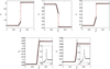 |
Fig. 1 Normalized density, x-velocity, plasma pressure, plasma temperature, and radiation energy profiles computed for the relaxed state of the hydrodynamic shock. The semi-analytic solution of Lowrie & Rauenzahn (2007) is also shown as a dashed red line. |
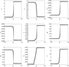 |
Fig. 2 Normalized density, x-velocity, y-velocity, z-velocity, plasma pressure, y-magnetic field, z-magnetic field, plasma temperature, and radiation energy density profiles computed for the relaxed state of the fast magnetosonic shock. |
4.2 Heating and cooling
Next, we test the process of energy exchange between plasma and radiation through the heating and cooling term  . A 2D stationary, non-magnetized plasma is considered with uniform properties and zero velocity. The density of the gas is taken to be ρ0 = 10−7 g/cm3. The adiabatic index is γ = 5/3, the opacity is κ = 0.4 cm2/g and the mean molecular weight is µ = 0.6. The computational domain consists of ten cells per direction. Initially, the plasma and radiation energies are out of radiative equilibrium, that is, the plasma and radiation temperatures are different. The total energy, that is, the sum of the plasma thermal energy and radiation energy, is initially taken to be (e0 + E0) = 1012 erg/cm3 . Given the total energy, for a given density, it is possible to find the equilibrium temperature, Teq, by equating the total energy to the sum of e = ρkBTeq/(mpµ) and
  . The corresponding plasma thermal energy at equilibrium is found out to be eequi = 6.89706 × 10⁷ erg/cm3. The thermal energy of the stationary plasma considered here would eventually reach this value, after exchanging energy with radiation through heating or cooling processes.
We consider two different scenarios in terms of the initial value of the plasma thermal energy density. In the first scenario, the initial plasma thermal energy is taken to be ei = 10−2eequi, that is, the plasma is cooler than the radiation and is expected to absorb energy from radiation through heating until radiative equilibrium is achieved. In the second scenario, we have ei = 102 eequi , and therefore the initially hotter plasma is expected to expel the excess energy through cooling and reach equilibrium. For both these conditions, the initial radiation energy density can be calculated by subtracting the initial plasma thermal energy density from the total energy density, that is, Ei = e0 + E0 − ei. We initialize the system with these values and let it relax until equilibrium is achieved. For the heating case, ei increases while Ei decreases with time, with both reaching their respective equilibrium values after some time. For the cooling case, the trend is opposite. Since for both scenarios ei ≪ 1012 erg/cm3, Ei stays ≈ 1012 erg/cm3 throughout the entire simulation. In this case, the radiation field is effectively a large reservoir, that plays the role of a heat source or sink. The time evolution of the plasma thermal energy density for both scenarios is shown on a logarithmic scale in Fig. 5, along with expected, semi-analytical evolution profiles. The case with ei = 102eequi seems to lag behind the semi-analytical solution in the beginning, that is, the plasma cools slower than expected. However, the observed solution eventually catches up with the semi-analytical solution and asymptotes to equilibrium at the expected rate. On the other hand, the case where ei = 10−2eequi seems to perfectly align with the semi-analytical solution. This test was also performed with a background uniform magnetic field, and it was verified that the presence of a uniform magnetic field makes no difference to the results.
4.3 Linear radiation-magnetohydrodynamic waves
It is well known that acoustic and, in general, magnetoacoustic waves may undergo damping when propagating in a radiative background field. Mihalas & Mihalas (1984) performed a linear perturbation analysis of the RHD equations in the optically thick diffusion limit. They derived a dispersion relation to quantify the damping rates of acoustic waves in a radiative medium. In this section we consider the magnetohydrodynamic generalization of such a dispersion relation for magnetoacoustic and Alfvén waves in a radiative medium. Traveling waves are then set up in a magnetized, radiative, stagnant background plasma and their various damping rates are observed. We then validate our simulation results by comparing the observed damping rates with those obtained analytically from the dispersion relation. We note that here we linearize the governing RMHD set about a static uniform medium, but more general linearizations about a 1D gravitationally stratified medium exist, as presented by Blaes & Socrates (2003). Our results connect directly with linear ideal MHD dispersion relations found in textbooks (Goedbloed et al. 2019), and may clarify the relation between the thermal instability resulting from optically thin radiative loss prescriptions (Claes & Keppens 2019) with the various unstable modes already identified in radiative media. For a complete derivation of the dispersion relation, the reader is referred to Appendix C.
This dispersion relation, as shown in Eq. (C.23), is a polynomial of order 8, as expected. For a uniform background medium and constant opacity κ, Eqs. (49) and (53) from Blaes & Socrates (2003) are equivalent to the above dispersion relation for the magnetohydrodynamic and hydrodynamic cases, respectively. We can clearly see that the dispersion relation factorizes into quadratic and hexic polynomials of ω. The quadratic polynomial factor gives the familiar Alfvén mode solution
 (30)
(30)
This means that the Alfvén mode has no imaginary component of ω and is therefore a simple forward and backward traveling wave without any exponential growth or decay. Therefore, in the current diffusion approximation, this mode is not influenced by the radiative terms (the reader is referred to the work by Driessen et al. (2020) demonstrating radiation-driven damping of Alfvén modes). The remaining six modes in Eq. (C.23) reduce to the standard MHD dispersion relation covering the (marginal) entropy mode, and the slow and fast pairs, augmented with a marginal frequency ω = 0 (the remnant of the radiative diffusion mode) if all radiative terms vanish (i.e., all derivatives of  vanish). In future work, it will be of interest to study how the thermal instability (related to the entropy mode, which can cause solar coronal condensations like prominences), and the added radiative diffusion mode relate in more general settings.
To use this dispersion relation to validate our RMHD implementation, we first considered, a static 1D weakly radiative plasma with plasma settings given by ρ0 = 3.216 × 10⁻⁹ g/cm3, P0 = 17.34 × 10³ erg/cm3 and B0 = (330.14, 0, 330.14) Gauss. The heat capacity ratio is γ = 5/3, and the mean molecular weight is µ = 0.5. The radiation energy density, E0 = 8.60834 × 10³ erg/cm3, can be obtained from the radiative equilibrium condition by equating the radiation temperature to the plasma temperature. The plasma beta is β = 1. The length of the computational domain is 40λw, where λw is the wavelength of the wave excited at the left boundary. The computational grid is made up of 3200 cells, and AMR was not used for this case. At the right-hand side boundary, a Dirichlet boundary condition is used for the radiation energy density, whereas Neumann boundary conditions are applied on all other properties. Using the code’s capacity to handle interior boundaries, we actually overwrite the first wavelength within the domain with the purely ideal MHD time-dependent linear wave solution for various kinds of right-traveling waves, as described below, and their interactions with the background radiation field are observed as they propagate to the right. For each of these waves, the wavenumber, k = 2π/λw, is chosen in such a way that for the constant background opacity, κ = 0.4 cm2/g, the optical depth given by  is 103. For the above values, λw = 7.77363 × 1011 cm, and therefore, k = 8.08269 × 10⁻¹² cm−1.
As a first test, an Alfvén wave is excited. The eigenfunctions for the Alfvén wave are obtained by setting ω/k to the background x-Alfvén speed shown in Eq. (C.22), and neglecting all heating and radiation terms. For this value of ω, and since By,0 = 0, we can fix the  perturbation, while the y-magnetic field perturbation can be obtained in terms of
  as
as  . Using these perturbations, the following wave settings were used at the left interior boundary of the domain:
 (31)
(31)
 (32)
(32)
All other perturbations are zero, that is,  . We used a non-dimensional
  value of 10−2. Figure 6 shows the propagation of the vy and By components of the Alfvén wave after it crossed the right-hand side boundary of the computational domain. As discussed earlier, the Alfvén solution is completely decoupled from the rest of the eigensystem. It is therefore unaffected by the radiation and heating terms and propagates across the domain without undergoing any damping or instability.
Similarly, in two separate tests, the fast and slow magne-tosonic waves were excited. The corresponding eigenfunctions were obtained by setting ω/k to the background ideal MHD fast or slow magnetosonic speed, depending on the case. These magnetosonic speeds are given by
 (33)
(33)
where the “+” sign is for the fast wave and the “−” sign is for the slow wave. For exciting these waves in a way that avoids gas (and hence radiation) temperature variations, the adiabatic sound speed cɡ, was replaced with the isothermal sound speed, ciso in the above equation. Again, the heating and radiation terms are neglected for setting up these eigenfunctions. Fixing with a simple sinusoidal plane wave  perturbation, all other perturbations can be written in terms of
  as follows:
 (34)
(34)
 (35)
(35)
 (36)
(36)
 (37)
(37)
For By,0 = 0, the  and
and  perturbations are both zero (i.e.,
  ). We use a non-dimensional
  value of 10−2 for both the fast and slow magnetosonic wave tests. For the given values of the background plasma properties, the dispersion relation can be solved and all roots can be quantified. These eight solutions are tabulated in Table 1 and shown on the complex eigenfrequency plane in the top panel of Fig. 7. The imaginary components of the ω solutions, corresponding to the slow and fast magnetosonic speeds are ωIm,slow = 7.05868 × 10⁻⁸ s−1 and ωIm,fast = 4.10666 × 10⁻⁷s−1, respectively. The analytical damping rate per unit length, ωIm/(ω/k) is therefore ωIm,slow/cS,0 = 5.61643 × 10⁻¹⁴cm−1 and ωIm,fast/cf,0 = 1.35347 × 10⁻¹³cm−1 for the slow and fast waves, respectively. Figures 8 and D.1 show the results for the fast and slow waves, respectively. The expected, theoretical damping of the density perturbation amplitude is also plotted along with the observed results. The observed and theoretical results show an excellent match, for both the slow and fast magnetosonic waves.
We next consider the damping of waves in a radiation-dominant 1D static background plasma. The initial plasma settings are ρ0 = 3.216 × 10⁻⁹ g/cm3, p0 = 43.35 × 10³ erg/cm3 and B0 = (330.14,0,330.14) Gauss. With the higher pressure, the initial radiation energy density is now E0 = 336.26331 × 10³ erg/cm3, according to the radiative equilibrium condition. All other parameters such as µ, γ, k,  , λw and κ are the same as in the weakly radiative case described above. The boundary conditions and the prescription for exciting the right-traveling waves are also the same. The computational domain is composed of 3200 cells. The solutions of the resultant dispersion relation, corresponding to these background conditions are tabulated in Table 2 and shown on the complex eigenfrequency plane in the bottom panel of Fig. 7. The analytical damping rate per unit length is now ωIm,slow/cs,0 = 8.64217 × 10⁻¹⁴cm−1 for the slow magnetosonic wave and ωIm,fast/cf,0 = 8.58803 × 10⁻¹³cm−1 for the fast magnetosonic wave. Since the damping is an order of magnitude higher for the fast wave, the computational domain used for the fast wave damping case is 10λw, opposed to 40λw for the slow case damping case. The ρ, vx and E solutions, superimposed with the theoretical damping, for the fast and slow waves are shown in Figs. 9 and D.2, respectively. For the slow wave, the case was run with a range of mesh resolutions (800, 1600, 2400 and 3200 cells), to observe the effect of grid sizes on the observed damping rates. A magnified version of the density solution from Fig. D.2 is shown in Fig. 10, showing a single half-cycle of the damped slow magnetosonic wave, along with the theoretical, expected damping of the wave amplitude. This is also superimposed with the corresponding results obtained using 800, 1600 and 2400 cells. It is observed that the crest of the half-cycle approaches the theoretical damped amplitude with increasing resolution. The % errors in the observed damping rates with respect to the theoretical rate, for these various grid resolutions, are plotted as a function of grid resolution in Fig. D.3.
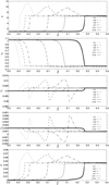 |
Fig. 3 Normalized density, x-velocity, y-velocity, z-velocity, and plasma pressure profiles computed for the moving fast magnetosonic shock at times t = 1.0, t = 2.0, t = 3.0, t = 7.0, t = 11.0, and t = 15.0. |
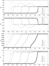 |
Fig. 4 Normalized y-magnetic field, ɀ-magnetic field, plasma temperature, and radiation energy density profiles computed for the moving fast magnetosonic shock at times t = 1.0, t = 2.0, t = 3.0, t = 7.0, t = 11.0, and t = 15.0. |
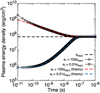 |
Fig. 5 Time evolution of plasma energy density for a plasma initialized with ei = 102eequi (cooling) and ei = 10−2eequi (heating). The red and blue dashed lines are the semi-analytical solutions for the cooling and heating cases, respectively. The black dashed line shows the equilibrium plasma thermal energy. Due to the logarithmic scaling of the time axis, the initial conditions at t = 0 are not seen here. |
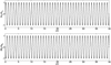 |
Fig. 6 Alfvén wave y-velocity (top) and y-magnetic field (bottom) perturbation components. |
Eigenfrequency solutions for the weakly radiative case.
Eigenfrequency solutions for the strongly radiative case.
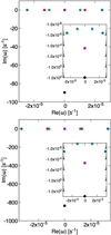 |
Fig. 7 Complex eigenfrequency plane showing the solutions (solid dots) to the dispersion relation in Eq. (C.23) forthe given background plasma properties and wavenumber. The top and bottom panels show the solutions for the weakly and strongly radiative cases, respectively. Green, red, blue, purple, and black show the slow, Alfvén, fast, thermal, and radiative diffusion modes, respectively. The inset plot shows all modes except the Alfvén mode using a logarithmic scale to compare the relative magnitudes ofthe imaginarycomponents oftheireigenfrequencies. |
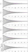 |
Fig. 8 Density, x-velocity, ɀ-velocity, plasma pressure, ɀ-magnetic field, and radiation energy density perturbation components for the fast magnetosonic wave for the weakly radiative background plasma. The analytical expected damping of the perturbation magnitude is also plotted as a solid purple line to allow for comparison with simulation results. |
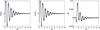 |
Fig. 9 Density, x-velocity, and radiation energy density perturbation components for the fast magnetosonic wave for the strongly radiative background plasma. The analytical expected damping of the perturbation magnitude is also plotted as a solid purple line to allow for comparison with simulation results. |
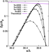 |
Fig. 10 Magnified version of the density solution from Fig. D.2 showing a single half cycle of the damped slow magnetosonic wave. The analytical expected damping of the perturbation magnitude is also plotted as a solid purple line. Corresponding results from coarser meshes comprising 800, 1600, and 2400 cells are also shown. |
4.4 Radiation-modified Riemann shock-tube problem
We move over to RMHD Riemann shock-tube problems in this section. We add radiation to two standard ideal MHD examples, namely the 1.5D case studied by Brio & Wu (1988), and the 1.75D case studied by Torrilhon (2003). The initial left and right states for both cases and their non-dimensional equivalent values are given in Table 3. All velocity components are zero initially for both cases. For the Brio-Wu case, the ɀ–magnetic fields are also zero. In this table, the physical length of the computational domain L, is also given for each case. A mean molecular weight of µ = 0.5 and a constant background opacity of κ = 400 cm2/g is used here. The adiabatic index is also listed. The initial computational grid is made up of 1024 cells, and seven AMR levels are used, leading to an effective resolution of 65 536 cells. Zero-gradient boundary conditions are applied at both boundaries for all variables. Without the radiation energy, these cases are identical to the ideal MHD cases by Brio & Wu (1988) and Torrilhon (2003), respectively. This can be clearly observed from the non-dimensional values in Table 3.
The solutions at time t = 4697.96 s for the radiative Brio-Wu case, equivalent to the non-dimensional value of t = 0.2, are shown in Fig. 11. The solid black line is the radiative solution with full FLD on, in order to allow the flow to switch between the optically thin (freestreaming) and optically thick (diffusion limit) regimes. The dot-dashed line is the radiative solution simulated in the diffusion limit. The non-radiative, ideal MHD solution by Brio & Wu (1988) is also shown as a solid red line for comparison, wherever applicable. This case consists of five waves from left to right: a fast rarefaction, a slow compound wave, a contact discontinuity, a slow shock, and a fast rarefaction wave. For the diffusion limit, the fast rarefaction to the right is replaced by a fast shock. Similarly, solutions for the radiative Torrilhon case, are shown in Fig. 12, for time t = 103.876 s, equivalent to the non-dimensional value of t = 0.4. As earlier,the solid black,dot-dashed and solid red lines represent the full-FLD, diffusion limit, and non-radiative solutions, respectively. The following seven waves are clearly detectable from left to right: a fast rarefaction, a rotational discontinuity, a slow rarefaction, a contact discontinuity, a slow magnetosonic shock, a rotational discontinuity, and finally a fast magnetosonic shock. Across the rotational discontinuities, the y- and ɀ- velocities and magnetic fields undergo a jump whereas the density, x–velocity, plasma pressure do not jump. The ɀ–velocity and ɀ–magnetic field do not change across the fast rarefaction wave towards the left. For both these cases, we observe that for the ideal MHD case, only the density jumps across the contact discontinuity whereas for the radiative case in the diffusion limit, the density and the plasma thermal pressure both jump. This major distinction between the non-radiative and radiative cases is due to the contribution of the radiation energy to total pressure. In the freestreaming (e.g., ideal MHD) limit, when λ = 0, the radiation passes freely through the plasma without exerting any pressure on the plasma and there is therefore no coupling between the radiation pressure and plasma momentum. On the other hand, in the diffusion limit, when λ = 1/3, the radiation exerts a radiation pressure of E/3 on the plasma and is thus strongly coupled with the plasma momentum. In this case, the effective total pressure experienced by the plasma is a sum of these pressure contributions, (p + E/3). Hence, across the contact discontinuity, the equilibrium force balance requires the sum (p + E/3) to remain unchanged. This explains the absence of a jump in (p + E/3) across contact discontinuities, as is observed in the diffusion limit solutions in Figs. 11 and 12, while the individual components p and E/3 both undergo jumps. With FLD, the coupling is partial, and the effective radiation pressure experienced by the plasma is less than E/3. We therefore see a jump in (p + E/3) across the contact discontinuity in the FLD solutions of Figs. 11 and 12.
Magnified versions of the density solutions, superimposed with the flux-limiter λ, and the radiation energy density solutions, superimposed with the AMR level, for the Brio-Wu test are shown in Fig. 13 for the full FLD case. The various wave locations are also marked here (dotted lines across the span of the rarefaction and compound waves, and dash-dot-dot lines for the discontinuities). Similar plots for the Torrilhon test are shown in Fig. 14, also including the By solution. For both tests, the AMR does a good job in capturing the various waves created, reaching the highest refinement level at the discontinuities. For both these tests, we observe that λ stays at its diffusion limit value of 1 /3 in regions with zero radiation energy density gradients, while showing clear variation at shocks and contact discontinuities. For the Torrilhon test, λ shows a spike also at the two rotational discontinuities. This is due to very small remaining variations in E, which are too small to be observed in Fig. 14. These arise due to the difficulty in the exact capturing of rotational discontinuities in the numerical schemes used. This is a challenge left for future work, as we do not expect any λ variation across them, where E should remain constant. This also necessitated the extreme use of AMR on this simple 1D experiment, as too low effective resolutions can show unphysical oscillatory behavior in especially λ (i.e., related to the gradient of E, which we evaluate numerically), as also impacted by the choice of limiter used in center-to-edge reconstructions. In the rarefaction regions, λ switches to its freestreaming value of ~0 for the Torrilhon case, while showing a smooth transition between the optically thick and thin regimes for the Brio-Wu case. We must note that the λ value also depends on the density, opacity and (dimensionalized) length scale of the problem. Higher values of these drive λ closer to the optically thick regime, while lower values bring it closer to the freestreaming regime.
Initial left and right states for RMHD Riemann problems.
4.5 Two-dimensional magnetoconvection with radiation
We simulate the case of two-dimensional compressible convection in the presence of a magnetic field, originally studied by Hurlburt & Toomre (1988), but here we also account for the effects of radiation. This scenario is relevant for the plasma motion inside the convective zone of the Sun, and the original study showed how an initial uniform vertical field gets swept into concentrated flux sheets, relevant for explaining the granular appearance of convective cells at the solar photosphere. This is a proof-of-principle simulation of an important multi-D effect that is present in the convective layers of stars. In these convective regions, energy transport through the stellar atmosphere is not necessarily carried by radiation, but also by convective transport. This convective transport effect can be altered or dampened due to the presence of magnetic fields as the fieldlines can constrict the motion of the convective cells. Understanding magnetoconvection is a crucial ingredient in our understanding of stellar envelopes. This magnetoconvection case requires physical effects such as viscous diffusion, magnetic diffusion (resistivity), anisotropic thermal conduction and external gravity.
Accounting for these effects, the governing equations are
 (38)
(38)
 (39)
(39)
 (40)
(40)
 (41)
(41)
Here, g is the gravitational acceleration vector, η is the magnetic diffusivity, K is the thermal conductivity, and τ is the viscous stress tensor given by
 (42)
(42)
where µɡ is the plasma’s dynamic viscosity. Also,  is the unit vector in direction of the magnetic field. For this case, we consider a 2D rectangular (x, y) domain of dimensionless length, Lx = 3, and depth Ly = 1. The depth is represented using a dimensionless depth variable d, where d = −y, that ranges from d = d0 at the top to d = d0 + 1 at the bottom, where d0 = 0.1. Initially the plasma is taken to be stagnant, that is, v(t = 0) = 0 everywhere. The magnetic field is initially vertical and uniform with a dimensionless value of By,0 = 6.573 × 10⁻². The non-dimensional initial profiles for temperature, density and pressure are given by Tɡ(d) = d, ρ(d) = d/d0, and p(d) = d2/d0, respectively. Therefore, at the top, (Tɡ, ρ, p)to p = (0.1, 1, 0.1), and at the bottom, (Tɡ, ρ, p)bot = (1.1, 11, 12.1). The Prandtl number, given by
 (43)
(43)
is taken to be unity, resulting in a constant anisotropic thermal conduction coefficient. The adiabatic index is γ = 5/3. The Chandrasekhar number given by
 (44)
(44)
is taken to be 72. The magnetic Prandtl number given by
 (45)
(45)
is taken to be 0.25. The non-dimensional gravitational acceleration is given by
 (46)
(46)
where ∇Tɡ is the initial non-dimensionalized vertical temperature gradient.
The dimensionalized length and depth of the domain are Lx = 3 × 108 cm and Ly = 108 cm. The dimensionalized values for the plasma properties are (Tɡ, ρ, p)top = (6000K, 3.61286 × 10⁻¹⁰ g/cm2, 3.57864 × 10² erg/cm3) at the top and (Tɡ, ρ, p)bot = (66000 K, 3.97415 × 10⁻⁹ g/cm2, 4.33016 × 10⁴ erg/cm3) at the bottom. The dimensionalized magnetic field becomes By,0 = 13.93887 Gauss. The externally applied gravitational field is ɡ = −989.53838 m/s2. Initially, radiative equilibrium is assumed everywhere, that is, the plasma and radiation temperatures are equal. Accordingly, the radiation energy density values at the top and bottom are Eto p = 9.80519 erg/cm3 and Ebottom = 1.43558 × 10⁵ erg/cm3, respectively. The corresponding non-dimensional values are Eto p = 2.73992 × 10⁻³ and Ebottom = 40.11518, respectively. An opacity of κ = 0.4 × 10⁻³ cm2/g is used for this case. Apart from the plasma density, the orders of magnitude of these values are representative of those in the convection zone of the Sun. The plasma density is approximately 103 times lower than the typical values in the convection zone of the Sun. Using density values similar to those in the Sun would proportionally increase the plasma pressure and reduce the significance of the radiation pressure. As the current work focuses on radiation-dominant cases, we stick to these density values.
The temperature is held fixed at the top boundary d = d0, and its vertical derivative is held fixed to unity at the bottom boundary, d = d0 + 1. The radiation temperature is held equal to the plasma temperature at both top and bottom boundaries. The horizontal magnetic field is held fixed at zero at the top and bottom boundaries. The magnetic field lines are forced to stay vertical there, but are free to move laterally and can exhibit compression or expansion. The vertical velocity, the vertical gradient of the horizontal velocity and the horizontal magnetic field all vanish at the top and bottom boundaries. Therefore, the horizontal components of the viscous and magnetic stresses also vanish at these boundaries. These boundary conditions can be summarized as
 (47)
(47)
Periodic boundary conditions are used at the left and right boundaries for all variables. To initiate the convective instability, small-amplitude velocity perturbations are introduced into the stagnant plasma. The above initial and boundary conditions, apart from those for the radiation energy, have been described in detail by Hurlburt & Toomre (1988).
The simulation is run for a non-dimensional time t = 500, corresponding to a dimensionalized physical time of 4.417 hours. AMR is driven by the Löhner’s criterion using gradients of density, pressure and radiation energy density. The very first high density downflows occurring due to convection are observed at around t = 9. Figure 15 shows the density profile at this time, with the adaptive mesh. The AMR captures these plumes very well. After the relatively high number of plumes, the flow settles into a dynamically steady, oscillatory state, marked by intermittent downflows and periodic compressions of the magnetic field. A typical solution at such a later time is also shown in Fig. 15 along with the mesh. Figure 16 shows a snapshot of the magnetic field lines at both these time instances, clearly showing how the initially uniform vertical magnetic field is swept into concentrated flux sheets by the convective flow. Figure 17 shows the ratios of the magnetic and radiation pressures to the plasma pressure at this later time. Animations depicting the time evolution for Figs. 15–17 are available online. Figure 18 shows the time-evolution of the total volume-integrated kinetic, magnetic, internal and radiation energies. In the bottom subfigure, it also shows the maximum current density, Jmax, superimposed along with the magnetic energy evolution. Before the onset of convection, the magnetic energy shows a flat profile until about t = 8. During this time, the kinetic energy shows an almost instantaneous increase at t = 0, due to the initial flow profile not being in vertical pressure equilibrium. This is because of the added radiation pressure on top of the original equilibrium initial conditions specified by Hurlburt & Toomre (1988). The vertical motions allow the plasma to equilibrate without affecting the magnetic field. After these initial transients, the magnetic field lines start to first compress, causing a sharp increase in the total magnetic energy. This increase coincides with an increase in kinetic energy, corresponding to the onset of convection. The magnetic energy then oscillates about an average value in a dynamically steady state. Loss of magnetic energy occurs due to decompression and due to the magnetic field being wound up by the flow and slowly getting dissipated away from the interior by reconnection. The internal and radiation energies settle down at about t = 400 to steady values and reach radiative equilibrium. Figure 19 shows the evolution of the grid coverage as a function of time, showing the proportion of the total area of the computational domain covered by the various AMR levels.
As this case involves the winding of the magnetic field by the convective plumes and the resultant magnetic reconnection, the use of the Linde method for divergence control can create significant errors in the discrete divergence in regions where such phenomena occur. As mentioned earlier, such monopole effects can lead to errors in the magnetic energy and thus also in the total energy, leading to artificial heating or cooling effects. It is therefore in our interest to examine such errors. The top panel in Fig. 20 shows the cell-integrated divergence at t = 9, obtained using the Linde method. This corresponds to the density flow solution and magnetic field lines shown in the top panels of the Figs. 15 and 16, respectively. For comparisons, this case was also run using several other divergence control methods, namely the Powell source term method (Powell et al. 1999), the CT method (Olivares et al. 2019), the Janhunen method (Janhunen 2000) and the Linde–Janhunen method. The discrete divergence for the Powell, Janhunen and Linde-Janhunen methods is also shown in the rest of the panels in Fig. 20. The Linde and Linde-Janhunen methods are observed to produce errors of somewhat lower magnitude as compared to the Powell and Janhunen methods. In this particular discretization, the CT method produces divergence errors of the order of machine precision zero. However, the CT method produces monopole errors similar to other schemes, when a different discretization is used for the evaluation of the divergence, and still contributes to artificial heating like other schemes.
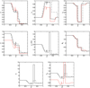 |
Fig. 11 Normalized density, x-velocity, y-velocity, plasma pressure, (plasma + radiation) pressure, y-magnetic field, radiation energy density, and plasma temperature solutions at t = 0.2 for Brio & Wu (1988)’s 1.5D Riemann shock-tube problem. Wherever applicable, the corresponding solution for the non-radiative case by Brio & Wu (1988) is also shown as a solid red line. The solutions we show in black are in full FLD (solid) or in diffusion limit (dot-dashed). |
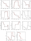 |
Fig. 12 Normalized density, x-velocity, y-velocity, ɀ-velocity, plasma pressure, (plasma + radiation) pressure, y-magnetic field, ɀ-magnetic field, radiation energy density, and plasma temperature solutions and the By versus Bɀ plot, at t = 0.4 for the Torrilhon (2003) 1.75D Riemann shock-tube problem. Wherever applicable, the corresponding solution for the non-radiative case by Torrilhon (2003) is also shown as a solid red line. The solutions we show in black are either in full FLD (solid) or in diffusion limit (dot-dashed). |
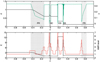 |
Fig. 13 Density (top) and radiation energy density (bottom) solutions for the full FLD radiative Brio-Wu test. The flux-limiter λ solution (green) is superimposed on the density solution, whereas the AMR level is superimposed on the radiation energy density solution. The dotted vertical lines span the rarefaction waves and the dash-dot-dot vertical lines mark discontinuities. In the top panel, the five waves formed are distinctly marked: fast rarefaction (FR), slow compound (SC) wave, contact discontinuity (CD), slow shock (SS), and fast rarefaction (FR) wave. |
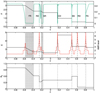 |
Fig. 14 Density (top), radiation energy density (middle), and y–magnetic field solutions for the full FLD radiative Torrilhon test. The flux-limiter λ solution (green) is superimposed on the density solution, whereas the AMR level is superimposed on the radiation energy density solution. The dotted vertical lines span the rarefaction waves and the dash-dot-dot vertical lines mark discontinuities. In the top panel, the seven waves formed are distinctly marked: fast rarefaction (FR), rotational discontinuity (RD), slow rarefaction (SR), contact discontinuity (CD), slow shock (SS), rotational discontinuity (RD), and fast shock (FS). |
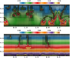 |
Fig. 15 Density for the radiative magnetoconvection case at t = 9 (top) and at t = 429 (bottom). |
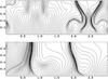 |
Fig. 16 Magnetic field lines for the radiative magnetoconvection case at t = 9 (top) and at t = 429 (bottom). |
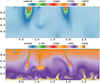 |
Fig. 17 Ratio of magnetic pressure (top) and radiation pressure (bottom) to plasma pressure at t = 429. |
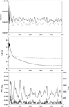 |
Fig. 18 Time evolutions for the diffusion limit radiative magnetoconvection test. Top: total kinetic energy (solid) and total magnetic energy (dash-dot). Middle: total radiation energy (solid) and total plasma internal energy (dash-dot). Bottom: total magnetic energy (solid) and maximum current density (dash-dot). |
5 Discussion and conclusions
This paper describes the recently added RMHD capabilities of the MPI-AMRVAC computational framework. To test this RMHD module, a variety of benchmark tests were designed, and several cases of radiation-dominated MHD shocks were simulated. We have extended on previous works (Mihalas & Mihalas 1984; Coggeshall & Axford 1986; Bouquet et al. 2000; Lowrie & Rauenzahn 2007; Lowrie & Edwards 2008) discussing the radiation-modified Rankine–Hugoniot jump conditions for hydrodynamical shocks in the diffusion limit to corresponding relations for RMHD shocks. We highlighted the various types of classical MHD shocks (fast, slow, intermediate, and switch-on) to modified versions in RMHD. These steady shocks were used to test the solver’s robustness, the capability of its AMR to capture strong shocks and discontinuities, and the handling of conserved quantities. We subsequently performed a linear perturbation analysis to derive the RMHD dispersion relations for the damping of magnetoacoustic waves in a radiative, magnetized static background plasma. The analytical damping rates for each of the characteristic waves (slow, fast, and undamped Alfvén) obtained from the dispersion relation also showed an excellent match with the rates obtained from numerical simulations. The radiation-modified versions of MHD Rie-mann shock-tube problems were simulated and used to present example cases involving transitions between optically thick to thin radiative conditions. By including a 1.75D problem from Torrilhon (2003), we demonstrated the effect of radiation on the various waves generated in an MHD system well, where the rotational discontinuities in particular are challenging to capture numerically. Although several researchers have performed RMHD simulations in the past, most targeted specific applications occurring in realistic astrophysical environments, which are not always easily reproduced. Our benchmark cases made deliberate simplifications (such as assuming constant opacities) in order to highlight the numerical challenges in RMHD settings, even in essentially 1D scenarios, requiring AMR. Through this paper, we also sought to address the scarcity of available literature on standard test cases for RMHD. All of the tests in this work can be used by future researchers to validate and test their codes. We also showed the potential to study the detailed interaction between convective and diffusive radiative flux transport in multi-dimensional setups in an idealized setting motivated by solar magnetoconvection.
The newly developed RMHD module of MPI-AMRVAC is now ready to be used to study more realistic scientific applications, such as the envelopes, atmospheres, and winds of massive stars with significant magnetic fields. Since the tests in this paper were quite basic, a constant value of the opacity, κ, was assumed. However, for realistic applications, more physically accurate models of plasma opacities will have to be used that account for opacity dependence on local plasma properties. For instance, the variation of opacities is crucial to simulate phenomena such as certain radiation-driven instabilities occurring in stellar atmospheres and luminous accretion discs (Blaes & Socrates 2003). As such, future work may involve relaxation of the constant opacity assumption and using opacity tables. For example, Moens et al. (2022a) and Debnath et al. (2024) have already demonstrated the use of opacity tables in MPI-AMRVAC’s RHD module for their study of Wolf–Rayet stars and O-stars, respectively. More realistic scientific applications could also involve studying regions of large radiation pressures and transition regions between optically thin and optically thick regimes. For such cases, numerical techniques such as the modified Godunov method of Miniati & Colella (2007) would help capture the coupling between the radiation and plasma momentum and energy terms better. Future work would also entail the implementation of such techniques.
For solar applications, the RMHD module demonstrated here can bridge the gap between coronal-only simulations, which have been the main research application for MPI-AMRVAC to date, and advanced RMHD simulations including optically thick convective layers. It will be of interest to clarify the connections between coronal condensations driven by optically thin prescriptions (as the entropy mode can turn into a thermal instability) and the more complete RMHD description with a radiative field incorporated and dynamically coupled to the plasma evolution. It may be necessary to develop a tailored solar atmosphere variation where the net heat-loss prescription,  , can be varied depending on temperature and optical thickness in order to smoothly connect the typical
  tabulated cooling curve Λ(T) variations applicable in the corona (see Hermans & Keppens 2021) with those obtained through the FLD prescriptions. We leave this for follow-up studies.
Although MPI-AMRVAC’s RMHD module is now ready to be used for scientific solar and astrophysical applications, the use of the FLD module must be approached with caution. The FLD has several potentially critical limitations (Mihalas & Mihalas 1984; Hayes & Norman 2003; Davis et al. 2012; Jiang et al. 2012), and its use must be carefully considered on a case-by-case basis. For example, FLD has been known to produce spurious solutions in transition regions; this has been observed in the accretion disk simulations of Boley et al. (2007). Inaccuracies of the FLD in accretion disk simulations have also been highlighted in the work of Davis et al. (2012). The FLD is a monochromatic frequency-independent approximation, and it can fail to accurately model radiative flows with a strong dependence on wave frequencies. A key aspect of the FLD model is that the radiation flux is assumed to be in the direction of the radiation energy density gradient rather than computed from the radiative transfer equation. Jiang et al. (2012) demonstrated a photon bubble instability simulation where the radiation flux direction is not aligned with the direction of the radiation energy density gradient at the generated shock fronts. The FLD assumption would clearly fail in such cases. This assumption can also introduce serious errors in optically thin regions that have highly anisotropic radiation fields. Therefore, the FLD method fails in capturing shadows and beams, as has been clearly demonstrated in the work of Hayes & Norman (2003) and Davis et al. (2012).
The FLD also forces the Eddington factor to strictly lie between one-third and one, whereas Jiang et al. (2012) demonstrated cases of radiative shocks where the Eddington factor can fall below one-third. The FLD approximation retains only the terms shown in the box in the radiation momentum equation, that is, Eq. (A.17). This relation between the divergence of the pressure tensor and the radiative flux is the basis for using Fick’s diffusion law as the closure relation. This removes the effect of radiation inertia from radiation flow solutions. Finally, the radiation pressure tensor is taken to be a diagonal tensor in the optically thick limit of the FLD model, with the off-diagonal terms being neglected. This eliminates effects such as radiation viscosity (Mihalas & Mihalas 1984; Castor 2004; Jiang et al. 2012). Both radiation inertia and radiation viscosity can play a significant role in the dynamics of accretion disk flows. More sophisticated radiation models could be used to improve on these limitations. For example, Jiang et al. (2012) clearly demonstrated the ability of the VET method to capture beams and shadows, in contrast to FLD. However, increasingly sophisticated models come with increased complexity and a higher computational cost. The possible incorporation of such models into MPI-AMRVAC’s RMHD module should be the subject of follow-up efforts. These efforts could then also involve more rigorous tests, such as the shadow test, beam test, and the photon bubble instability test as well as applications such as accretion disk simulations.
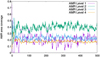 |
Fig. 19 Grid coverage (proportion of total area) for the various AMR levels. |
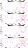 |
Fig. 20 Magnetic field discrete divergence error for the radiative magnetoconvection case at t = 9 for the (top to bottom) Linde, Janhunen, Linde-Janhunen, and Powell methods. |
Data availability
The movies associated to Fig. 15-17 are available at https://www.aanda.org
Acknowledgements
R.K. is supported by an FWO project G0B9923N and received funding from the European Research Council (ERC) under the European Union Horizon 2020 research and innovation program (grant agreement No. 833251 PROMINENT ERC-ADG 2018). RK acknowledges KU Leuven C1 project C16/24/010 UnderRadioSun. A.u.-D. acknowledges NASA ATP grant number 80NSSC22K0628 and support by NASA through Chandra Award number TM4-25001A issued by the Chandra X-ray Observatory 27 Center, which is operated by the Smithsonian Astrophysical Observatory for and on behalf of NASA under contract NAS8-03060. JS and NM acknowledge the support of the European Research Council (ERC) Horizon Europe grant under grant agreement number 101044048. A.u.-D. and JS acknowledge support from the Belgian Research Foundation Flanders (FWO) Odysseus program under grant number G0H9218N. The authors thank the referee, Dr. Lizhong Zhang, for valuable feedback that greatly improved the manuscript.
Appendix A Frame transformation for the radiation-magnetohydrodynamic equations
Following Jiang et al. (2012), the radiation MHD equations, including the equations of the radiation energy density and radiation flux, with the radiative terms evaluated in the inertial lab frame, are given by
 (A.1)
(A.1)
 (A.2)
(A.2)
 (A.3)
(A.3)
 (A.4)
(A.4)
 (A.5)
(A.5)
 (A.6)
(A.6)
Here, ELF , FLF and PLF are the frequency-integrated radiation energy density, flux vector and pressure tensor in the inertial lab frame. The source terms in the momentum and plasma energy equations are given by
 (A.7)
(A.7)
 (A.8)
(A.8)
Here, κP, κE, κF and κS , are the Planck, energy density, flux mean absorption and flux mean scattering opacities, respectively. The relations between the radiation energy density, flux vector and pressure tensor in the inertial and co-moving frames are
 (A.9)
(A.9)
 (A.10)
 (A.11)
where ECMF, FCMF and PCMF are the frequency-integrated radiation energy density, flux vector and pressure tensor in the co-moving frame.
Equations (A.1) and (A.4) are identical to Eqs. (1) and (4), respectively. Substituting Eqs. (A.7)–(A.11) in Eqs. (A.2), (A.3), (A.5), and (A.6), assuming κS = 0, and substituting
 (A.12)
 (A.13)
 (A.14)
 (A.15)
 (A.16)
 (A.17)
Here, O(v/c) comprises terms proportional to (v/c) or higher order powers. For non-relativistic velocities, these terms are very small and can be conveniently neglected. For non-relativistic velocities, and dropping the subscript CMF for simplicity, the Eqs. (A.14), (A.15), and (A.16) reduce to Eqs. (2), (3), and (8), respectively. In Eq. (A.17), the terms with the (1/c2) factor on the left-hand side and the higher order terms are ignored, resulting in the relation between the divergence of the pressure tensor and the radiative flux as shown in the box drawn.
Appendix B Test cases: Radiation-modified steady shocks in the diffusion limit
Rankine-Hugoniot jump conditions for RMHD shocks.
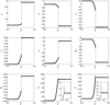 |
Fig. B.1 Normalized density, x-velocity, y-velocity, ɀ-velocity, plasma pressure, y-magnetic field, ɀ-magnetic field, plasma temperature, and radiation energy density profiles computed for the relaxed state of the slow magnetosonic shock. |
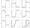 |
Fig. B.2 Normalized density, x-velocity, y-velocity, ɀ-velocity, plasma pressure, y-magnetic field, ɀ-magnetic field, plasma temperature, and radiation energy density profiles computed for the relaxed state of the intermediate magnetosonic shock. |
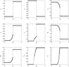 |
Fig. B.3 Normalized density, x-velocity, y-velocity, ɀ-velocity, plasma pressure, y-magnetic field, ɀ-magnetic field, plasma temperature, and radiation energy density profiles computed for the relaxed state of the slow switch-off magnetosonic shock. |
Appendix C Dispersion relation for damping of magnetohydrodynamic waves in a radiative medium
To obtain the dispersion relation, we first rewrite the Eqs. (1)–(4) in non-conservative form, and reformulate the energy equation to a pressure evolution equation:
 (C.1)
(C.1)
 (C.2)
(C.2)
 (C.3)
(C.3)
 (C.4)
(C.4)
These above equations will be linearized assuming an infinite, static, time-independent (∂/∂t = 0), uniform background for the plasma properties. In this equilibrium state, the heating and cooling function  is also assumed to vanish, and therefore the equilibrium radiation temperature equals the plasma temperature. The equilibrium radiation force fr also vanishes due to the constant radiation energy. The equilibrium state is hereby denoted by ρ0, v0 = 0, p0, B0, Tg,0, E0 and Tr,0 = Tg,0 for the equilibrium density, velocity, plasma pressure, magnetic field, plasma temperature, radiation energy density and radiation temperature, respectively. Small linear deviations from this equilibrium are denoted by the subscript ‘1’. The linearized versions of Eqs. (C.1)–Eqs. (C.4) for λ = 1/3 (the optically thick limit) are given by
 (C.5)
(C.5)
 (C.6)
(C.6)
 (C.7)
(C.7)
 (C.8)
(C.8)
 (C.9)
(C.9)
 (C.10)
 (C.11)
Here,  are partial derivatives of the
  function with respect to ρ, Tr, and Tg, respectively, and are given by
 (C.12)
 (C.13)
 (C.14)
These derivatives are to be evaluated for the background state such that  , as we have adopted radiative equilibrium. We note that we here get rather simple expressions for these derivatives, as we assumed constant opacities κ, while many of the physically relevant unstable wave mode solutions in stellar interiors or atmospheres relate to detailed variations of opacities with density and temperatures. This complication is, for instance, handled in Blaes & Socrates (2003). The relation between radiation energy density and radiation temperature can be linearized to give
 (C.15)
To obtain dispersion relations for linear stability analysis, plane-wave perturbations of the form
 (C.16)
can be assumed, where k is the wavenumber and ω is the angular frequency for the plane wave perturbation. For the 1.75D cases studied numerically further on, we chose k to be along the x-axis k = (k, 0,0).
Applying such perturbations to ρ, v, p, B, and E and substituting them in Eqs. (C.5)–(C.8) and (C.11) gave the following:
 (C.17)
 (C.18)
 (C.19)
 (C.20)
 (C.21)
Equations (C.17)–(C.21) originally constitute a set of nine equations, accounting for each of the three dimensions of the momentum and magnetic field eigenvalue equations. However, for k = (k, 0,0), the equation for the x-component of the magnetic field reduces to  , reducing it to a set of eight equations. This is the solenoidality condition for the perturbed magnetic field, and it makes the number of physical eigenfrequencies ω to be eight in total, one more than the familiar ideal MHD result. In the above equations,
  can be substituted in terms of density and plasma pressure perturbation amplitudes using Eq. (C.10). Similarly, Ê can be substituted using Eq. (C.15).
The above equations then lead to the dispersion relation, where we used certain characteristic speeds of the flow:
 (C.22)
where cg,0, cr,0, vA,0 and vA,x,0 are the adiabatic plasma sound speed, the radiation sound speed, the total Alfvén speed and the x-Alfvén speed, respectively. The final dispersion relation can be written as:
 (C.23)
Appendix D Test cases: Linear radiation-magnetohydrodynamic waves
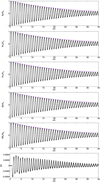 |
Fig. D.1 Density, x-velocity, ɀ-velocity, plasma pressure, ɀ-magnetic field and radiation energy density perturbation components of the slow magnetosonic wave for the weakly radiative background plasma. The analytical expected damping of the perturbation magnitude is also plotted as a solid purple line, for comparison with simulation results. |
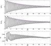 |
Fig. D.2 Density, x-velocity, and radiation energy density perturbation components of the slow magnetosonic wave for the strongly radiative background plasma. The analytical expected damping of the perturbation magnitude is also plotted as a solid purple line, for comparison with simulation results. |
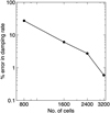 |
Fig. D.3 Percent error in the observed damping rates with respect to the theoretical rate of the slow magnetosonic wave damped by a strongly radiative background plasma. |
References
- Alme, M. L., & Wilson, J. R. 1974, ApJ, 194, 147 [Google Scholar]
- Blaes, O., & Socrates, A. 2003, ApJ, 596, 509 [CrossRef] [Google Scholar]
- Bloch, H., Tremblin, P., González, M., Padioleau, T., & Audit, E. 2021, A&A, 646, A123 [NASA ADS] [CrossRef] [EDP Sciences] [Google Scholar]
- Boley, A. C., Durisen, R. H., Nordlund, Å., & Lord, J. 2007, ApJ, 665, 1254 [Google Scholar]
- Bouquet, S., Teyssier, R., & Chieze, J. P. 2000, ApJS, 127, 245 [Google Scholar]
- Brio, M., & Wu, C. C. 1988, J. Computat. Phys., 75, 400 [Google Scholar]
- Carlsson, M., Hansteen, V. H., Gudiksen, B. V., Leenaarts, J., & De Pontieu, B. 2016, A&A, 585, A4 [NASA ADS] [CrossRef] [EDP Sciences] [Google Scholar]
- Cassinelli, J. P. 1979, Annu. Rev. Astron. Astrophys., 17, 275 [Google Scholar]
- Castor, J. I. 2004, Radiation hydrodynamics (Cambridge University Press) [CrossRef] [Google Scholar]
- Castor, J. I., Abbott, D. C., & Klein, R. I. 1975, ApJ, 195, 157 [Google Scholar]
- Claes, N., & Keppens, R. 2019, A&A, 624, A96 [NASA ADS] [CrossRef] [EDP Sciences] [Google Scholar]
- Coggeshall, S. V., & Axford, R. A. 1986, Phys. Fluids, 29, 2398 [Google Scholar]
- Commerçon, B., Teyssier, R., Audit, E., Hennebelle, P., & Chabrier, G. 2011, A&A, 529, A35 [NASA ADS] [CrossRef] [EDP Sciences] [Google Scholar]
- Davis, S. W., Stone, J. M., & Jiang, Y.-F. 2012, ApJS, 199, 9 [NASA ADS] [CrossRef] [Google Scholar]
- Debnath, D., Sundqvist, J., Moens, N., et al. 2024, A&A, 684, A177 [NASA ADS] [CrossRef] [EDP Sciences] [Google Scholar]
- Dedner, A., Kemm, F., Kröner, D., et al. 2002, J. Computat. Phys., 175, 645 [Google Scholar]
- Donné, D., & Keppens, R. 2024, ApJ, 971, 90 [CrossRef] [Google Scholar]
- Driessen, F. A., Kee, N. D., Sundqvist, J. O., & Owocki, S. P. 2020, MNRAS, 499, 4282 [CrossRef] [Google Scholar]
- Druett, M., Ruan, W., & Keppens, R. 2024, A&A, 684, A171 [NASA ADS] [CrossRef] [EDP Sciences] [Google Scholar]
- Einfeldt, B. 1988, SIAM J. Numer. Anal., 25, 294 [CrossRef] [MathSciNet] [Google Scholar]
- Emerick, A., Bryan, G. L., & Mac Low, M.-M. 2018, ApJ, 865, L22 [NASA ADS] [CrossRef] [Google Scholar]
- Esseldeurs, M., Siess, L., De Ceuster, F., et al. 2023, A&A, 674, A122 [NASA ADS] [CrossRef] [EDP Sciences] [Google Scholar]
- Farcy, M., Rosdahl, J., Dubois, Y., Blaizot, J., & Martin-Alvarez, S. 2022, MNRAS, 513, 5000 [NASA ADS] [CrossRef] [Google Scholar]
- Flock, M., Fromang, S., González, M., & Commerçon, B. 2013, A&A, 560, A43 [NASA ADS] [CrossRef] [EDP Sciences] [Google Scholar]
- Fornberg, B. 1988, Math. Computat., 51, 699 [Google Scholar]
- Goedbloed, H., Keppens, R., & Poedts, S. 2019, Magnetohydrodynamics of Laboratory and Astrophysical Plasmas (Cambridge University Press) [Google Scholar]
- Gonzalez, M., Audit, E., & Huynh, P. 2007, A&A, 464, 429 [CrossRef] [EDP Sciences] [Google Scholar]
- González, M., Vaytet, N., Commerçon, B., & Masson, J. 2015, A&A, 578, A12 [NASA ADS] [CrossRef] [EDP Sciences] [Google Scholar]
- Hayes, J. C., & Norman, M. L. 2003, ApJS, 147, 197 [NASA ADS] [CrossRef] [Google Scholar]
- Hayes, J. C., Norman, M. L., Fiedler, R. A., et al. 2006, ApJS, 165, 188 [NASA ADS] [CrossRef] [Google Scholar]
- Hermans, J., & Keppens, R. 2021, A&A, 655, A36 [NASA ADS] [CrossRef] [EDP Sciences] [Google Scholar]
- Hurlburt, N. E., & Toomre, J. 1988, ApJ, 327, 920 [Google Scholar]
- Igumenshchev, I. V., Narayan, R., & Abramowicz, M. A. 2003, ApJ, 592, 1042 [Google Scholar]
- Iijima, H., & Yokoyama, T. 2017, ApJ, 848, 38 [NASA ADS] [CrossRef] [Google Scholar]
- Jacoutot, L., Kosovichev, A., Wray, A., & Mansour, N. 2008, ApJ, 684, L51 [NASA ADS] [CrossRef] [Google Scholar]
- Janhunen, P. 2000, J. Computat. Phys., 160, 649 [Google Scholar]
- Jenkins, J. M., & Keppens, R. 2022, Nat. Astron., 6, 942 [NASA ADS] [CrossRef] [Google Scholar]
- Jerčić, V., Jenkins, J., & Keppens, R. 2024, A&A, 688, A145 [NASA ADS] [CrossRef] [EDP Sciences] [Google Scholar]
- Jiang, Y.-F., & Blaes, O. 2020, ApJ, 900, 25 [NASA ADS] [CrossRef] [Google Scholar]
- Jiang, Y.-F., Stone, J. M., & Davis, S. W. 2012, ApJS, 199, 14 [NASA ADS] [CrossRef] [Google Scholar]
- Jiang, Y.-F., Stone, J. M., & Davis, S. W. 2014, ApJ, 784, 169 [NASA ADS] [CrossRef] [Google Scholar]
- Jiang, Y.-F., Blaes, O., Stone, J. M., & Davis, S. W. 2019a, ApJ, 885, 144 [NASA ADS] [CrossRef] [Google Scholar]
- Jiang, Y.-F., Stone, J. M., & Davis, S. W. 2019b, ApJ, 880, 67 [Google Scholar]
- Johnson, B. M., & Klein, R. I. 2010, JQSRT, 111, 723 [Google Scholar]
- Keppens, R., Nool, M., Tóth, G., & Goedbloed, J. 2003, Comput. Phys. Commun., 153, 317 [NASA ADS] [CrossRef] [Google Scholar]
- Keppens, R., Meliani, Z., van Marle, A. J., et al. 2012, J. Computat. Phys., 231, 718 [Google Scholar]
- Keppens, R., Braileanu, B. P., Zhou, Y., et al. 2023, A&A, 673, A66 [NASA ADS] [CrossRef] [EDP Sciences] [Google Scholar]
- Khomenko, E., Vitas, N., Collados, M., & De Vicente, A. 2018, A&A, 618, A87 [NASA ADS] [CrossRef] [EDP Sciences] [Google Scholar]
- Kim, J.-G., Kim, W.-T., Ostriker, E. C., & Skinner, M. A. 2017, ApJ, 851, 93 [NASA ADS] [CrossRef] [Google Scholar]
- Levermore, C., & Pomraning, G. 1981, ApJ, 248, 321 [NASA ADS] [CrossRef] [Google Scholar]
- Li, X., Keppens, R., & Zhou, Y. 2022, ApJ, 926, 216 [NASA ADS] [CrossRef] [Google Scholar]
- Li, X., Keppens, R., & Zhou, Y. 2023, ApJ, 947, L17 [NASA ADS] [CrossRef] [Google Scholar]
- Linde, T. 2002, Int. J. Numer. Methods Fluids, 40, 391 [Google Scholar]
- Liu, X.-D., Osher, S., & Chan, T. 1994, J. Computat. Phys., 115, 200 [NASA ADS] [CrossRef] [Google Scholar]
- Löhner, R. 1987, Comput. Methods Appl. Mech. Eng., 61, 323 [CrossRef] [Google Scholar]
- Lowrie, R. B., & Edwards, J. D. 2008, Shock waves, 18, 129 [Google Scholar]
- Lowrie, R. B., & Rauenzahn, R. M. 2007, Shock waves, 16, 445 [Google Scholar]
- Mihalas, D., & Mihalas, B. 1984, Foundations of Radiation Hydrodynamics (New York: Oxford University) [Google Scholar]
- Minerbo, G. N. 1978, JQSRT, 20, 541 [Google Scholar]
- Miniati, F., & Colella, P. 2007, J. Computat. Phys., 224, 519 [Google Scholar]
- Modestov, M., Khomenko, E., Vitas, N., et al. 2024, Solar Phys., 299, 23 [Google Scholar]
- Moens, N., Poniatowski, L., Hennicker, L., et al. 2022a, A&A, 665, A42 [NASA ADS] [CrossRef] [EDP Sciences] [Google Scholar]
- Moens, N., Sundqvist, J., El Mellah, I., et al. 2022b, A&A, 657, A81 [NASA ADS] [CrossRef] [EDP Sciences] [Google Scholar]
- Nóbrega-Siverio, D., Martinez-Sykora, J., Moreno-Insertis, F., & Carlsson, M. 2020, A&A, 638, A79 [NASA ADS] [CrossRef] [EDP Sciences] [Google Scholar]
- Ohsuga, K., Mineshige, S., Mori, M., & Kato, Y. 2009, PASJ, 61, L7 [NASA ADS] [Google Scholar]
- Olivares, H., Porth, O., Davelaar, J., et al. 2019, A&A, 629, A61 [NASA ADS] [CrossRef] [EDP Sciences] [Google Scholar]
- Panja, M., Cameron, R., & Solanki, S. K. 2020, ApJ, 893, 113 [CrossRef] [Google Scholar]
- Porth, O., Xia, C., Hendrix, T., Moschou, S., & Keppens, R. 2014, ApJS, 214, 4 [NASA ADS] [CrossRef] [Google Scholar]
- Powell, K. G., Roe, P. L., Linde, T. J., Gombosi, T. I., & De Zeeuw, D. L. 1999, J. Computat. Phys., 154, 284 [Google Scholar]
- Przybylski, D., Cameron, R., Solanki, S., et al. 2022, A&A, 664, A91 [NASA ADS] [CrossRef] [EDP Sciences] [Google Scholar]
- Ruan, W., Xia, C., & Keppens, R. 2020, ApJ, 896, 97 [NASA ADS] [CrossRef] [Google Scholar]
- Ruan, W., Yan, L., & Keppens, R. 2023, ApJ, 947, 67 [NASA ADS] [CrossRef] [Google Scholar]
- Ruan, W., Keppens, R., Yan, L., & Antolin, P. 2024, ApJ, 967, 82 [CrossRef] [Google Scholar]
- Shakura, N. I., & Sunyaev, R. A. 1973, A&A, 24, 337 [NASA ADS] [Google Scholar]
- Skinner, M. A., & Ostriker, E. C. 2013, ApJS, 206, 21 [NASA ADS] [CrossRef] [Google Scholar]
- Stein, R., & Nordlund, Å. 1998, ApJ, 499, 914 [NASA ADS] [CrossRef] [Google Scholar]
- Stein, R. F., & Nordlund, Å. 2000, Solar Phys., 192, 91 [Google Scholar]
- Stone, J. M., & Norman, M. L. 1992, ApJS, 80, 753 [Google Scholar]
- Teunissen, J., & Keppens, R. 2019, Comput. Phys. Commun., 245, 106866 [Google Scholar]
- Tomida, K., Tomisaka, K., Matsumoto, T., et al. 2010, ApJ, 714, L58 [NASA ADS] [CrossRef] [Google Scholar]
- Tomida, K., Tomisaka, K., Matsumoto, T., et al. 2012, ApJ, 763, 6 [Google Scholar]
- Tomida, K., Okuzumi, S., & Machida, M. N. 2015, ApJ, 801, 117 [Google Scholar]
- Torrilhon, M. 2003, J. Plasma Phys., 69, 253 [NASA ADS] [CrossRef] [Google Scholar]
- Turner, N., & Stone, J. 2001, ApJS, 135, 95 [NASA ADS] [CrossRef] [Google Scholar]
- Turner, N. J., Stone, J. M., Krolik, J. H., & Sano, T. 2003, ApJ, 593, 992 [NASA ADS] [CrossRef] [Google Scholar]
- Van der Holst, B., Tóth, G., Sokolov, I. V., et al. 2011, ApJS, 194, 23 [Google Scholar]
- Vink, J. S. 2024, arXiv e-prints [arXiv:2406.16517] [Google Scholar]
- Wünsch, R. 2024, Front. Astron. Space Sci., 11, 1346812 [Google Scholar]
- Xia, C., & Keppens, R. 2016, ApJ, 823, 22 [Google Scholar]
- Xia, C., Chen, P., & Keppens, R. 2012, ApJ, 748, L26 [Google Scholar]
- Xia, C., Keppens, R., Antolin, P., & Porth, O. 2014a, ApJ, 792, L38 [Google Scholar]
- Xia, C., Keppens, R., & Guo, Y. 2014b, ApJ, 780, 130 [Google Scholar]
- Xia, C., Teunissen, J., El Mellah, I., Chané, E., & Keppens, R. 2018, ApJS, 234, 30 [Google Scholar]
- Yang, X., & Yuan, F. 2012, PASJ, 64, 69 [Google Scholar]
- Zel’dovich, Y. B., & Raizer, Y. P. 1967, Physics of shock waves and high- temperature hydrodynamic phenomena (New York: Academic) [Google Scholar]
- Zhou, Y.-H., Xia, C., Keppens, R., Fang, C., & Chen, P. 2018, ApJ, 856, 179 [Google Scholar]
All Tables
All Figures
|
Fig. 1 Normalized density, x-velocity, plasma pressure, plasma temperature, and radiation energy profiles computed for the relaxed state of the hydrodynamic shock. The semi-analytic solution of Lowrie & Rauenzahn (2007) is also shown as a dashed red line. |
| In the text | |
|
Fig. 2 Normalized density, x-velocity, y-velocity, z-velocity, plasma pressure, y-magnetic field, z-magnetic field, plasma temperature, and radiation energy density profiles computed for the relaxed state of the fast magnetosonic shock. |
| In the text | |
|
Fig. 3 Normalized density, x-velocity, y-velocity, z-velocity, and plasma pressure profiles computed for the moving fast magnetosonic shock at times t = 1.0, t = 2.0, t = 3.0, t = 7.0, t = 11.0, and t = 15.0. |
| In the text | |
|
Fig. 4 Normalized y-magnetic field, ɀ-magnetic field, plasma temperature, and radiation energy density profiles computed for the moving fast magnetosonic shock at times t = 1.0, t = 2.0, t = 3.0, t = 7.0, t = 11.0, and t = 15.0. |
| In the text | |
|
Fig. 5 Time evolution of plasma energy density for a plasma initialized with ei = 102eequi (cooling) and ei = 10−2eequi (heating). The red and blue dashed lines are the semi-analytical solutions for the cooling and heating cases, respectively. The black dashed line shows the equilibrium plasma thermal energy. Due to the logarithmic scaling of the time axis, the initial conditions at t = 0 are not seen here. |
| In the text | |
|
Fig. 6 Alfvén wave y-velocity (top) and y-magnetic field (bottom) perturbation components. |
| In the text | |
|
Fig. 7 Complex eigenfrequency plane showing the solutions (solid dots) to the dispersion relation in Eq. (C.23) forthe given background plasma properties and wavenumber. The top and bottom panels show the solutions for the weakly and strongly radiative cases, respectively. Green, red, blue, purple, and black show the slow, Alfvén, fast, thermal, and radiative diffusion modes, respectively. The inset plot shows all modes except the Alfvén mode using a logarithmic scale to compare the relative magnitudes ofthe imaginarycomponents oftheireigenfrequencies. |
| In the text | |
|
Fig. 8 Density, x-velocity, ɀ-velocity, plasma pressure, ɀ-magnetic field, and radiation energy density perturbation components for the fast magnetosonic wave for the weakly radiative background plasma. The analytical expected damping of the perturbation magnitude is also plotted as a solid purple line to allow for comparison with simulation results. |
| In the text | |
|
Fig. 9 Density, x-velocity, and radiation energy density perturbation components for the fast magnetosonic wave for the strongly radiative background plasma. The analytical expected damping of the perturbation magnitude is also plotted as a solid purple line to allow for comparison with simulation results. |
| In the text | |
|
Fig. 10 Magnified version of the density solution from Fig. D.2 showing a single half cycle of the damped slow magnetosonic wave. The analytical expected damping of the perturbation magnitude is also plotted as a solid purple line. Corresponding results from coarser meshes comprising 800, 1600, and 2400 cells are also shown. |
| In the text | |
|
Fig. 11 Normalized density, x-velocity, y-velocity, plasma pressure, (plasma + radiation) pressure, y-magnetic field, radiation energy density, and plasma temperature solutions at t = 0.2 for Brio & Wu (1988)’s 1.5D Riemann shock-tube problem. Wherever applicable, the corresponding solution for the non-radiative case by Brio & Wu (1988) is also shown as a solid red line. The solutions we show in black are in full FLD (solid) or in diffusion limit (dot-dashed). |
| In the text | |
|
Fig. 12 Normalized density, x-velocity, y-velocity, ɀ-velocity, plasma pressure, (plasma + radiation) pressure, y-magnetic field, ɀ-magnetic field, radiation energy density, and plasma temperature solutions and the By versus Bɀ plot, at t = 0.4 for the Torrilhon (2003) 1.75D Riemann shock-tube problem. Wherever applicable, the corresponding solution for the non-radiative case by Torrilhon (2003) is also shown as a solid red line. The solutions we show in black are either in full FLD (solid) or in diffusion limit (dot-dashed). |
| In the text | |
|
Fig. 13 Density (top) and radiation energy density (bottom) solutions for the full FLD radiative Brio-Wu test. The flux-limiter λ solution (green) is superimposed on the density solution, whereas the AMR level is superimposed on the radiation energy density solution. The dotted vertical lines span the rarefaction waves and the dash-dot-dot vertical lines mark discontinuities. In the top panel, the five waves formed are distinctly marked: fast rarefaction (FR), slow compound (SC) wave, contact discontinuity (CD), slow shock (SS), and fast rarefaction (FR) wave. |
| In the text | |
|
Fig. 14 Density (top), radiation energy density (middle), and y–magnetic field solutions for the full FLD radiative Torrilhon test. The flux-limiter λ solution (green) is superimposed on the density solution, whereas the AMR level is superimposed on the radiation energy density solution. The dotted vertical lines span the rarefaction waves and the dash-dot-dot vertical lines mark discontinuities. In the top panel, the seven waves formed are distinctly marked: fast rarefaction (FR), rotational discontinuity (RD), slow rarefaction (SR), contact discontinuity (CD), slow shock (SS), rotational discontinuity (RD), and fast shock (FS). |
| In the text | |
|
Fig. 15 Density for the radiative magnetoconvection case at t = 9 (top) and at t = 429 (bottom). |
| In the text | |
|
Fig. 16 Magnetic field lines for the radiative magnetoconvection case at t = 9 (top) and at t = 429 (bottom). |
| In the text | |
|
Fig. 17 Ratio of magnetic pressure (top) and radiation pressure (bottom) to plasma pressure at t = 429. |
| In the text | |
|
Fig. 18 Time evolutions for the diffusion limit radiative magnetoconvection test. Top: total kinetic energy (solid) and total magnetic energy (dash-dot). Middle: total radiation energy (solid) and total plasma internal energy (dash-dot). Bottom: total magnetic energy (solid) and maximum current density (dash-dot). |
| In the text | |
|
Fig. 19 Grid coverage (proportion of total area) for the various AMR levels. |
| In the text | |
|
Fig. 20 Magnetic field discrete divergence error for the radiative magnetoconvection case at t = 9 for the (top to bottom) Linde, Janhunen, Linde-Janhunen, and Powell methods. |
| In the text | |
|
Fig. B.1 Normalized density, x-velocity, y-velocity, ɀ-velocity, plasma pressure, y-magnetic field, ɀ-magnetic field, plasma temperature, and radiation energy density profiles computed for the relaxed state of the slow magnetosonic shock. |
| In the text | |
|
Fig. B.2 Normalized density, x-velocity, y-velocity, ɀ-velocity, plasma pressure, y-magnetic field, ɀ-magnetic field, plasma temperature, and radiation energy density profiles computed for the relaxed state of the intermediate magnetosonic shock. |
| In the text | |
|
Fig. B.3 Normalized density, x-velocity, y-velocity, ɀ-velocity, plasma pressure, y-magnetic field, ɀ-magnetic field, plasma temperature, and radiation energy density profiles computed for the relaxed state of the slow switch-off magnetosonic shock. |
| In the text | |
|
Fig. D.1 Density, x-velocity, ɀ-velocity, plasma pressure, ɀ-magnetic field and radiation energy density perturbation components of the slow magnetosonic wave for the weakly radiative background plasma. The analytical expected damping of the perturbation magnitude is also plotted as a solid purple line, for comparison with simulation results. |
| In the text | |
|
Fig. D.2 Density, x-velocity, and radiation energy density perturbation components of the slow magnetosonic wave for the strongly radiative background plasma. The analytical expected damping of the perturbation magnitude is also plotted as a solid purple line, for comparison with simulation results. |
| In the text | |
|
Fig. D.3 Percent error in the observed damping rates with respect to the theoretical rate of the slow magnetosonic wave damped by a strongly radiative background plasma. |
| In the text | |
Current usage metrics show cumulative count of Article Views (full-text article views including HTML views, PDF and ePub downloads, according to the available data) and Abstracts Views on Vision4Press platform.
Data correspond to usage on the plateform after 2015. The current usage metrics is available 48-96 hours after online publication and is updated daily on week days.
Initial download of the metrics may take a while.