| Issue |
A&A
Volume 693, January 2025
|
|
|---|---|---|
| Article Number | A224 | |
| Number of page(s) | 11 | |
| Section | Stellar atmospheres | |
| DOI | https://doi.org/10.1051/0004-6361/202452375 | |
| Published online | 21 January 2025 | |
Suppression of photospheric velocity fluctuations in strongly magnetic O stars in radiation-magnetohydrodynamic simulations
1
Penn State Scranton,
120 Ridge View Drive,
Dunmore,
PA
18512,
USA
2
Instituut voor Sterrenkunde, KU Leuven,
Celestijnenlaan 200D,
3001
Leuven,
Belgium
3
Centre for mathematical Plasma Astrophysics, Department of Mathematics, KU Leuven,
Celestijnenlaan 200B,
3001
Leuven,
Belgium
★ Corresponding author; This email address is being protected from spambots. You need JavaScript enabled to view it.
Received:
26
September
2024
Accepted:
14
December
2024
Abstract
Context. O stars generally show clear signs of strong line broadening (in addition to rotational broadening) in their photospheric absorption lines (typically referred to as macroturbulence), believed to originate in a turbulent sub-surface zone associated with enhanced opacities due to the recombination of iron-group elements (at T ~ 150–200 kK). O stars with detected global magnetic fields also display such macroturbulence; the sole exception to this is NGC 1624-2, which also has the strongest (by far) detected field of the known magnetic O stars. It has been suggested that this lack of additional line broadening is due to NGC 1624-2’s exceptionally strong magnetic field, which might be able to suppress the turbulent velocity field generated in the iron opacity peak zone.
Aims. We tested this hypothesis based on two-dimensional (2D), time-dependent, radiation magnetohydrodynamical (RMHD) box- in-a-star simulations for O stars that encapsulate the deeper sub-surface atmosphere (down to T ~ 400 kK), the stellar photosphere, and the onset of the supersonic line-driven wind in one unified approach. To study the potential suppression of atmospheric velocity fluctuations, we extended our previous non-magnetic O star radiation-hydrodynamic (RHD) simulations to include magnetic fields of varying strengths and orientations.
Methods. We used MPI-AMRVAC, which is a Fortran 90 based publically available parallel finite volume code that is highly modular. We used the recently added RMHD module to perform all our simulations here.
Results. For moderately strong magnetic cases (~1 kG), the simulated atmospheres are highly structured and characterised by large root-mean-square velocities, and our results are qualitatively similar to those found in previous non-magnetic studies. By contrast, we find that a strong horizontal magnetic field in excess of 10 kG can indeed suppress the large velocity fluctuations, and can thus stabilise (and thereby also inflate) the atmosphere of a typical early O star in the Galaxy. On the other hand, an equally strong radial field is only able to suppress horizontal motions, and as a consequence these models exhibit significant radial fluctuations.
Conclusions. Our simulations provide an overall physical rationale as to why NGC 1624-2 with its strong ~20 kG dipolar field lacks the large macroturbulent line broadening that all other known slowly rotating early O stars exhibit. However, our simulations also highlight the importance of field geometry for controlling the atmospheric dynamics in massive and luminous stars that are strongly magnetic, tentatively suggesting latitudinal dependence of macroturbulence and basic photospheric parameters.
Key words: instabilities / magnetohydrodynamics (MHD) / stars: atmospheres / stars: magnetic field / stars: massive / stars: winds, outflows
© The Authors 2025
 Open Access article, published by EDP Sciences, under the terms of the Creative Commons Attribution License (https://creativecommons.org/licenses/by/4.0), which permits unrestricted use, distribution, and reproduction in any medium, provided the original work is properly cited.
This article is published in open access under the Subscribe to Open model. This email address is being protected from spambots. You need JavaScript enabled to view it. to support open access publication.
1 Introduction
Optical absorption-line spectroscopy of O stars has revealed that rotation is not the only macroscopic broadening mechanism at play in their atmospheres (e.g. Conti & Ebbets 1977; Howarth et al. 1997; Simón-Díaz et al. 2017). The additional broadening component is typically very broad, for early O stars the full width at half maximum (FWHM) values are ~50–100 km/s, and often have a Gaussian-like shape. When a spectrum is fitted by means of a 1D model atmosphere code, it is included as an ad hoc very large macroturbulence (Simón-Díaz & Herrero 2007; Sundqvist et al. 2013; Simón-Díaz et al. 2017). However, modern multi-dimensional radiation-hydrodynamic (RHD) atmospheric simulations (Jiang et al. 2015; Schultz et al. 2022; Debnath et al. 2024) and earlier theoretical studies (e.g. Cantiello et al. 2009; Grassitelli et al. 2015) demonstrate that such large turbulent velocity fields naturally occur in the envelopes of luminous O stars.
In these models, the atmospheric structure originates in a radiatively and convectively unstable region located slightly beneath the stellar surface, at temperatures T ~ 150–200 kK, associated with a peak in the Rosseland mean opacity due to recombination effects of iron-group elements (Rogers & Iglesias 1992). Due to the enhanced opacities, local pockets of gas in this sub-surface region receive a radiation force that can locally exceed the inward gravitational pull and be strongly accelerated upwards, towards the upper atmosphere, where they further interact with the line-driven outflow (Castor et al. 1975) that is initiated from just above the variable optical photosphere (Debnath et al. 2024). This complex interplay then creates large photospheric turbulent velocities, typically of order vturb ~ 50– 100 km/s for early and luminous O stars in the Galaxy (Jiang et al. 2015; Debnath et al. 2024). Recent spectral synthesis performed directly from such multi-D models have shown that the typical widths of observed absorption line profiles can indeed be quite well matched (Schultz et al. 2022).
In parallel with this development, spectropolarimetric observations have revealed that ~7–10% of massive main-sequence stars possess strong magnetic fields (Wade et al. 2012a; Grunhut et al. 2017). The detected fields are large-scale, ordered, often with a dominant dipole component, and stable over long timescales. As such, their origin is not related to any possible dynamo mechanism operating in their atmospheres; instead, they are believed to be surviving fossil fields (Jermyn & Cantiello 2020), which potentially may be related to stellar mergers (Schneider et al. 2019). Interestingly, magnetic O stars are also very slow rotators, which likely is a result of strong magnetic braking in their powerful line-driven wind outflows (e.g. ud-Doula et al. 2009).
Sundqvist et al. (2013) used the fact that rotational broadening is negligible in magnetic O stars to empirically investigate the occurrence of turbulent motions in their atmospheres, from an analysis of their optical absorption lines. They found that the only magnetic O star that did not possess significant macroscopic line broadening was NGC 1624-2, which is also the O star with the strongest (by far) detected magnetic field. Specifically, NGC 1624-2 has an inferred dipole magnetic field of ~20 kG, whereas the other magnetic O stars have fields ~1 kG (Wade et al. 2012b). Using simple scaling analysis arguments, it was then suggested that the atmosphere of NGC 1624-2 might be stabilised against velocity fluctuations since even at the iron opacity peak it was estimated that magnetic pressure should be higher than the gas pressure (see also MacDonald & Petit 2019; Jermyn & Cantiello 2020). On the other hand, for the other magnetic O stars (with an order of magnitude weaker fields), equipartition should already occur very near the stellar surface, well above the iron opacity bump zone. As such, the fluctuations leading to macroturbulence in these stars would not be suppressed, in agreement with observations of their absorption line profiles.
This mechanism for magnetic inhibition of turbulent motion would then be analogous to that believed to occur in the magnetic and chemically peculiar Ap stars (Michaud 1970; Landstreet 1998), with the key difference that for O stars the turbulence originates in a sub-surface instability zone associated with iron recombination. More specifically, in Ap stars the magnetic fields are believed to inhibit convective motion in the atmosphere, leading to chemical stratification (Michaud 1970). This process allows heavy elements like iron and rare earths to accumulate in localised regions, which manifests in their unique spectral lines. The suppression of turbulence by magnetic fields in the atmosphere is central to the development of these chemical peculiarities. In these stars the magnetic field disrupts the mixing in their atmospheres, allowing diffusion processes to separate elements and create the observed overabundances. In this context, it may also be worth mentioning that although instabilities originate beneath the surface for O stars, numerical simulations show that the resulting turbulent zones extend up to the stellar photosphere and into the wind (Jiang et al. 2015; Schultz et al. 2022; Debnath et al. 2024). How potential suppression of this turbulence by a strong magnetic field might affect chemical abundance patterns in this regime remains an open question.
Jiang et al. (2017) computed multi-dimensional RMHD models of massive-star envelopes covering the iron opacity bump region, focusing on field strengths up to 1 kG. They found that such fields were not able to suppress the very large characteristic turbulent velocities associated with corresponding non-magnetic simulations. For this paper we tested whether even stronger magnetic fields (up to 20 kG) are indeed able to inhibit atmospheric velocity fluctuations in O stars, based on 2D simplified models that preclude any dynamo effects that can lead to further magnetic field amplifications. We utilised recently developed methods of RHD simulations for hot, luminous, and massive star atmospheres (Moens et al. 2022; Debnath et al. 2024) and extend them to include initially uniform magnetic field with fixed orientation. In Sect. 2, we discuss our numerical methods including initial and boundary conditions. We present the simulation results in Sect. 3, and a general discussion in Sect. 4, before a short summary is given in Sect. 5.
2 Simulation methods
Based on initial 3D simulations of Wolf–Rayet outflows by Moens et al. (2022), Debnath et al. (2024) conducted timedependent two-dimensional (2D) simulations of O-star atmospheres using a flux-limited diffusion (FLD) RHD finite volume grid in a ‘box-in-a-star’ configuration, including line-driving opacities and corrections for spherical divergence. Building on that work, we extended the analysis by incorporating an initially uniform magnetic field of different strengths threading the atmosphere of a representative early O star in the Galaxy.
2.1 Radiation-magnetohydrodynamics
All our models were performed using MPI-AMRVAC which is a Fortran 90-based parallel code often used for magnetohydrodynamics (MHD) simulations of solar and astrophysical plasmas (Keppens et al. 2012; Porth et al. 2014; Xia et al. 2018; Keppens et al. 2023). MPI-AMRVAC is highly modular with options for different numerical schemes and switches to include various physics terms in the governing equations enabling users to integrate newer modules into the existing code with relative ease. Most recently, Moens et al. (2022) have implemented FLD approach in MPI-AMRVAC to couple the hydrodynamics module with radiation. For this work, we extended this FLD approach to include equations of MHD. Details of this numerical scheme can be found in Narechania et al. (2024), but we briefly summarise some key points here for convenience.
MPI-AMRVAC numerically solves the RMHD equations on finite volume meshes in conservative form. These equations, consisting of the equations of conservation of mass, momentum, energy, and magnetic flux, including the effect of radiation and gravity in the form of source terms, are given by
 (1)
(1)
 (2)
(2)
 (3)
(3)
 (4)
(4)
Here ρ is the plasma density, v is the plasma velocity, p is the plasma pressure, B is the magnetic field, I is the identity tensor, fr is the radiation force described below, and fgrav is the gravitational force of a point stellar mass M⋆:
 (5)
(5)
The total energy, e, is the sum of the kinetic, internal and magnetic energies and is given by
 (6)
(6)
where γ is the adiabatic index of the gas. The ideal gas law given by
 (7)
(7)
provides the closure relation between the plasma temperature, pressure, and density. Here mp is proton mass, µ is the mean molecular weight, Tg is the plasma temperature, and kB is the Boltzmann constant. Throughout this paper we assume constant µ = 0.61 and γ = 5/3 (see also Debnath et al. 2024).
Additionally, the magnetic field must also satisfy the divergence-free condition:
 (8)
(8)
For the purpose of the current work, the discrete divergence is maintained using the Powell source term method (Powell 1994).
The fr term seen in the momentum equation is the radiation force written as
 (9)
(9)
where c is the speed of light, F is the radiation flux vector, and κF is the flux mean opacity. The  term in the energy equation is the term describing the plasma’s interaction with radiation through heating and cooling, and is given by
 (10)
(10)
Here E is the radiation energy density, κP is the Planck opacity, κE is the energy density opacity, and σ is the Stefan-Boltzmann constant. Since fr and  are both dependent on the radiation field, we also need a conservation equation for the radiation energy density. This equation is given by the frequency-integrated zeroth angular moment of the radiative transfer equation:
 (11)
(11)
This equation is written in the co-moving frame of the fluid, due to the ease of computing opacities in this frame, as opposed to an inertial frame of reference. Here P is the radiation pressure tensor and P : ∇v is the ‘photon tiring’ term.
The FLD-approximation by Levermore & Pomraning (1981) is used to close the radiation flux vector F:
 (12)
(12)
For the flux limiter λ, we employ the analytic relation
 (13)
(13)
as proposed by Levermore & Pomraning (1981). Here the dimensionless radiation energy density gradient, R, is given by
 (14)
(14)
This limiter λ ensures that the radiation flux does not exceed the physical limit, cE, in the optically thin free-streaming limit. On the other hand, for the diffusion limit, the accurate F = −c∇E/(3ρκ) is recovered.
Finally, P is evaluated as a function of E as
 (15)
(15)
where f is the Eddington tensor, as proposed by Turner & Stone (2001). The numerical methods used to evaluate all the above terms are described in detail in Moens et al. (2022). Rigorous testing of the new RMHD module is realised in Narechania et al. (2024). We used the magnetic field splitting technique in the RMHD module as described in Xia et al. (2018) (and references therein). As in previous work (Moens et al. 2022; Debnath et al. 2024), we assumed flux, energy, and Planck opacities to be equal, and computed opacities following the hybrid formalism by Poniatowski et al. (2022). This combines tabulated Rosseland means for deeper sub-surface layers with line-driving opacities effective in optically thin parts of the atmosphere. The finite- disc effect of line-driving (Pauldrach et al. 1986) is included following Debnath et al. (2024).
Fundamental parameters for the 〈2D〉 O-star model studied in this paper.
2.2 Numerical grid
All our simulations presented here use a Cartesian mesh. Although MPI-AMRVAC has the option for adaptive mesh refinement (AMR), we performed all our models using a fixed static grid with 128 in radial direction and 64 points in horizontal direction. For our box-in-a-star model of an O star atmosphere, we used the same stellar parameters as employed by Debnath et al. (2024) for their O4 star model, as shown in Table 1. Thus, we set the lower boundary to a fixed radius R0 = 13.54 R⊙, yielding a lower boundary temperature T0 ~ 450 kK deep inside the stellar envelope to model the entire iron opacity bump region. Our aim is to study atmospheric velocity fluctuations generated in the stellar envelope. Thus, we limited the outer boundary in the radial direction to r = 2 R0. This relatively small range also ensures that our assumption of uniform magnetic field within the box is reasonable. The horizontal coordinate covers a range from −0.25 R0 to 0.25 R0.
2.3 Initial and boundary conditions
For our initial and boundary conditions in all the simulations presented here, we again closely followed the procedure outlined in Debnath et al. (2024), to which we refer for more details. In brief, we assume a spherically symmetric, stationary, and analytic wind structure approximated by a β velocity law and mass density according to an initial assumed mass-loss rate. An analytic wind is smoothly connected to a lower atmosphere assumed to be in hydrostatic and thermal equilibrium. The magnetic field is uniform throughout the computational domain.
Boundary conditions for MHD models can often be challenging. Here, in the horizontal direction, boundaries are assumed to be periodic for all conserved quantities. At the lower boundary, the density is held constant as defined by the initial conditions, and the values for the ghost cells are extrapolated assuming hydrostatic equilibrium. The gas momentum is free to vary and is extrapolated from the first active cell to the ghost cells under the assumption of mass conservation. The radiation energy density (Erad) is extracted from its gradient by using Eq. (12) with a fixed input radiative luminosity at the lower boundary.
At the outer boundary, outflow boundary conditions are applied for all quantities except for Erad, which is analytically solved from the outer boundary radius to r → ∞, as described in Moens et al. (2022) and Debnath et al. (2024). However, the focus of this work is not on the stellar wind itself, and therefore further details of the wind outflow are not addressed in this paper.
2.4 Parameter study
To investigate the minimum magnetic field strength required suppressing the turbulence in the sub-surface region of an O4 atmosphere, we conducted numerical simulations with uniform magnetic fields of 1 kG, 10 kG, and 20 kG, oriented in both directions, radial and horizontal. The magnetic field configurations were introduced at time t = 0 in a computational domain that evolved for approximately nine physical days, which is about 20 dynamical timescales if we assume a typical macroturbulence velocity of 300 km s−1 in the sub-surface layer. By directly comparing these magnetic simulations1 to a non-magnetic control model, our aim was to identify the critical magnetic field threshold necessary to stabilise the atmospheric dynamics.
3 Simulation results
3.1 Classification of models
Our 2D simulations here specify mass, radius, and radiative luminosity at the lower boundary. Both the photospheric radius and the effective temperature Teff (defined at the average photospheric radius R*, where the mean optical depth τ ≈ 2/3) are emergent properties. Following the methodology of Debnath et al. (2024), we selected a model representative of a typical O4 star.
Keeping this model fixed, we only varied the strength and topology of the uniform magnetic field. We grouped our models into three categories based on the strength of the magnetic field: (i) weak B ~ 100 G, (ii) moderately strong B ~ 1 kG, and (iii) strong B ≥ 10 kG. These fields can be either in the radial or horizontal direction. In our local approach, they thus represent magnetic polar (radial) and equatorial (horizontal) viewing angles for an external observer.
In the non-magnetic O4 simulation presented by Debnath et al. (2024), structure starts appearing just below the iron opacity peak at ~200 kK where the gas becomes subject to convective, radiative, and also Rayleigh-Taylor instabilities (Blaes & Socrates 2003; van der Sijpt et al., in prep.). Local pockets of gas there experience radiative accelerations that exceed gravity, so that they shoot up from these deep layers into the upper and cooler atmosphere. In the upper atmospheric parts, Rosseland mean opacities are lower than in the deeper layers, meaning the plasma is decelerated. While some gas particles then indeed turn over and fall back into the deep atmosphere, others become subject to line-driving opacities, and are thus re-accelerated in the region around and just above the variable optical photosphere (launching an average supersonic wind outflow). This complex interplay creates large velocity dispersions (≳100 km/s for the case studied here) in the photospheric layers of such O-star RHD simulations. These large velocity dispersions provide significant turbulent pressure support; energy transport by enthalpy (=convection) is very inefficient in these luminous O-star atmospheres. For the case discussed here, radiative enthalpy is much higher than gas enthalpy, but still only provides ≲10% of the total energy transport even at the peak of the iron opacity bump, with the rest of the energy being carried by diffuse radiation. On the other hand, the large velocity dispersions give rise to high photospheric turbulent pressure, typically of the same order as the radiation pressure and significantly higher than the gas pressure, with associated turbulent velocities  that in turn are of the same order as the measured velocity dispersions (see Fig. 16 in Debnath et al. 2024, and the corresponding definitions in their Sect. 4.1).
While the analytic closure relation in our FLD approximation method is physically correct for deep optically thick layers, we note that it is only an approximation in regions where the atmosphere transitions from optically thick to optically thin, which may affect our predicted photospheric velocity dispersions. For those transitional regions, it would be desirable to instead apply a closure relation based on numerical solutions to the radiative transfer equation, as in the variable Eddington tensor (VET) models by Jiang et al. (2017). On the other hand, those simulations then do not include the effects of line-driving, which for O stars have a very strong impact on the dynamics near and above the stellar surface (Puls et al. 2008; Debnath et al. 2024). Since even 1D stationary atmospheric models accounting properly for such line-driving are very computationally expensive (Sander et al. 2017; Sundqvist et al. 2019) because of the complicated frequency-dependence of flux-weighted line opacities, it remains a challenge to include this effect in VET methods applied to multi-D simulations. However, since the focus here is on investigating whether a strong magnetic field can suppress velocity fluctuations originating in deep optically thick layers, we expect that our overall results should be fairly unaffected by these radiative transfer complications, at least qualitatively. This seems to also be supported by the overall qualitative agreement between our simulations and those by Jiang et al. (2017). Specifically, our simulations with weak magnetic fields closely resemble those of our corresponding non-magnetic model, though the former exhibits a slight increase in velocity dispersion in the sub-surface layers. This minor enhancement in turbulent velocity fluctuations for massive stars with weak magnetic fields qualitatively aligns with the findings of Jiang et al. (2017), who observed similar behaviour in their study. Since the aim here is to examine whether stronger magnetic fields can suppress such atmospheric velocity fluctuations, we focus primarily on discussing our simulation runs with stronger fields in this paper.
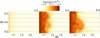 |
Fig. 1 Illustrative temporal evolution of a magnetic model with a 1 kG radial magnetic field. The colour scale represents the logarithm of density in cgs units, while the blue lines depict the magnetic field lines. Beginning with a spherically symmetric initial condition (left panel) threaded by a uniform magnetic field in radial direction, the model develops significant density and velocity variations after two to four days (middle panel; time = 3 d) and maintains them until the end of the simulation at approximately nine days (right panel; time = 6 d). |
3.2 Basic characteristics of magnetic simulations
Figure 1 shows a typical temporal evolution of our moderately strong magnetic (B = 1 kG) model with the initial magnetic field oriented in the radial direction. The plots show the logarithm of density plotted against the spatial coordinates normalised to lower boundary radius spatial coordinates. The blue lines represent the magnetic field.
After approximately one day of evolution, the model develops density and velocity fluctuations in a way similar to the process described above for the non-magnetic simulations. As both gas and radiation pressures are higher than the magnetic pressure, clear deviations from the radial topology emerge as the model progresses. In these 1 kG simulations, the magnetic field is not sufficiently strong to suppress turbulent motion in the deeper sub-surface layers near the iron opacity peak. This is also evident from the significant deformation of magnetic field lines observed in the later stages of evolution (right two panels of Figure 1). For weak magnetic cases (B < 100 G), such deformations of magnetic field lines are even more extreme, and the overall evolution closely resembles that of the non-magnetic case. These results are broadly consistent with the 3D RMHD models presented by Jiang et al. (2017).
Figure 2 presents the logarithm of density for the final snapshot of each simulation, taken after approximately nine days of evolution, for all magnetic field models. By this stage all simulations have reached a quasi-steady or quasi-periodic state, with no discernible influence from the initial conditions. For a direct comparison, the left column depicts the corresponding non-magnetic case. Progressing to the right, the models feature increasing magnetic field strengths of 1, 10, and 20 kG. The top row displays models with a radial magnetic field, while the bottom row shows those with a horizontal magnetic field orientation.
For the 1 kG models, regardless of whether the magnetic field is oriented radially or horizontally, strong velocity and density fluctuations remain a dominant feature throughout the simulation. This also suggests that moderately strong magnetic fields are insufficient to suppress the convective and radiative instabilities driving this extensive structure development in the sub-surface layers. The field may perturb the flow, but it lacks the strength to significantly alter the gas dynamics and suppress the strong turbulent motions.
In contrast, the behaviour changes substantially in the strong magnetic field models. When the magnetic field is aligned radially, it effectively suppresses horizontal gas motions, but permits piston-like oscillatory motions along the radial direction. These motions operate on a timescale of about half a day, indicating a dynamic balance where the magnetic field restricts turbulent flows, but allows for periodic compressions and expansions of the gas. This is likely related to the interplay between magnetic pressure and gas pressure in largely confining the flow along the field lines. This also might be the result of the 2D nature of our simulations that artificially imposes symmetry in the third dimension.
For models with strong horizontal magnetic fields, the suppression is even more pronounced. Here the magnetic field restricts both radial and horizontal motions, effectively quenching significant atmospheric structure from developing. The horizontal orientation of the field here clearly inhibits the vertical gas motions that drive large velocity fluctuations, leading to a more stable envelope that more closely resembles a radiative and strongly magnetic, quasi-hydrostatic stellar atmosphere. This almost complete suppression of velocity fluctuations in the strong horizontal field cases indicates that magnetic tension in these configurations is able to dominate the gas dynamics, suppressing the instabilities that would otherwise lead to large velocity dispersions.
Figure 3 illustrates the horizontally averaged density, plotted on a logarithmic scale, for all models as a function of the modified radial coordinate (x ≡ 1 − R0/r) over time. This representation emphasises the sub-surface layers, which are the primary focus of this study. The dashed black line marks the location of the average photosphere (Rphot), while the solid black line indicates the approximate position of the iron opacity peak, estimated at a temperature of T = 1.6 × 10⁵ K. Except for the model with the strongest horizontal magnetic field, all simulations show significant fluctuations between the iron opacity peak and Rphot. For reference, the leftmost column depicts the non-magnetic model, providing a baseline for comparison with the magnetic field models.
Figure 4 is analogous to Figure 3, but it depicts the radial velocity instead. The velocity fluctuations in all models clearly originate in the iron opacity bump region, as expected (Jiang et al. 2015; Debnath et al. 2024). Notably, in models with a radial magnetic field orientation, the stellar surface undergoes pistonlike oscillations. In contrast, models with a strong horizontal magnetic field configuration suppress these motions, preventing such oscillatory behaviour. Our results demonstrate that on timescales of a few hours, radial magnetic fields do not effectively inhibit the up-and-down piston-like motions observed in the gas, mirroring the oscillatory behaviour also seen in the simulations (with weaker fields) by Jiang et al. (2017). Conversely, strong horizontal magnetic fields can effectively suppress these oscillations.
Table 2 summarises the basic emergent stellar parameters for our models, including the stellar radius Rphot ≡ r(τ = 2/3), effective temperature Teff, and T0, the average temperature where magnetic and gas pressures are equal. Notably, models with moderately strong magnetic fields (both radial and horizontal) exhibit properties similar to the non-magnetic case. We do note a small deflation of the stellar envelope (i.e. a slightly smaller stellar radius) for the radial-field 1 kG case as compared to the 0G run (consistent with Jiang et al. 2017). This is in sharp contrast to the significant envelope inflation found for the runs with strong horizontal magnetic fields; this is discussed further in Sect. 4.
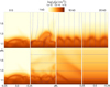 |
Fig. 2 Similar to Fig. 1, but comparing the late evolutionary states between the non-magnetic case (left column) and various magnetic models. The second column from the right shows models with a 1 kG magnetic field in the radial (top row) and horizontal (bottom row) directions. The third and fourth columns display models with 10 kG and 20 kG magnetic fields, respectively. |
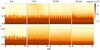 |
Fig. 3 Horizontally averaged density profiles as a function of time, using the modified radial coordinate x (≡ r − R0/r). The leftmost column serves as a non-magnetic reference. The top row displays models with radial magnetic fields of 1, 10, and 20 kG, while the bottom row shows models with horizontal magnetic fields of the same strengths. The dotted black line indicates the photospheric radius (r(τ = 2/3)), and the solid black line marks the location of the iron opacity peak (T ~ 1.6e5 K). |
Horizontally time-averaged values of Rphot, Teff, log(g), and T0 (estimated temperature where magnetic and gas pressure are equal to each other) for all the models in this study.
3.3 Suppression of motions in models with varying magnetic field strength and geometry
To further illustrate the effects of magnetic field strength and orientation, Figure 5 presents the root mean square (RMS) of radial (top panels) and tangential (bottom panels) velocity perturbations (vrms) for the different simulation models as a very simple proxy for the strength of photospheric velocity fluctuations. These time-averaged RMS values were computed over approximately the final three days of the simulation to ensure that the results are not influenced by transients from the initial conditions, thereby reflecting the quasi-steady or quasi-periodic state of the atmosphere.
In the left column the data correspond to simulations with a radial magnetic field orientation, while the right column depicts results for models with a horizontal magnetic field orientation. The differences in RMS velocities highlight the strong dependence of vrms on the magnetic field strength and configuration. It is apparent from these panels that, in general, the models with strong radial magnetic fields (dotted and dot-dashed lines) demonstrate a clear suppression of horizontal gas motion, while the models with strong horizontal magnetic fields (right column, top panel) inhibit radial gas movement.
Notably, for models with radial magnetic fields, the RMS radial velocity perturbations (vr,ms) remain around 100 km/s across all cases, regardless of magnetic field strength. However, the situation is different for the RMS of tangential velocity perturbations (vt,rms). The model with a weaker 1 kG radial magnetic field (green dashed line) fails to suppress turbulence in the region of the iron opacity peak, leading to elevated tangential velocity perturbations (vt,rms ≈ 100 km/s), which are comparable to the values seen in the non-magnetic reference model (blue line). However, for the stronger 10 kG case the value of vt,rms decreases to ~10 km/s, while for the strongest radial magnetic field case (20 kG) it falls even further, approaching or even falling below 1 km/s.
In contrast, the situation reverses for models with horizontal magnetic field orientation (right column). In these models, the radial gas motion is largely unaffected in the 1 kG case, where vr,rms hovers around 100 km/s. For stronger magnetic fields (>10 kG), however, vr,rms is reduced to values below 10 km/s. As for tangential velocity perturbations, all the models except the strongest magnetic field case exhibit vt,rms values near 100 km/s. It is only the strongest horizontal magnetic field model (20 kG) that successfully suppresses significant velocity fluctuations in both radial and horizontal directions, marking a significant distinction from other models.
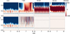 |
Fig. 4 Horizontally averaged radial velocity vr plotted as modified radial coordinate x (≡ r − R0/r) vs. time. The leftmost column represents the non-magnetic case for a direct comparison. The top row shows models with a radial magnetic field of 1, 10, and 20 kG. Similarly, the bottom panels show models with a horizontal magnetic field of 1, 10, and 20 kG. The dotted black line represents the photospheric radius (Rphot ≡ r(τ = 2/3) and the solid black line denotes the location of the iron opacity peak (T ~ 1.6 × 10⁵ K). The radial magnetic field does not inhibit up-and-down piston-like motions of the gas, whereas the strong horizontal magnetic field can fully suppress it. This figure also demonstrates clearly how velocity dispersion is initiated near the iron opacity peak (solid black line). We show only the final ~3 d of simulation for all models. Coincidentally, the model with 1 kG radial magnetic field was caught in one of the episodes of outbursts, which is also visible in Fig. 3, albeit less prominently. |
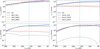 |
Fig. 5 Root mean square (RMS) values of radial (top panels) and tangential velocity perturbations (bottom panels) are shown for selected magnetic models as a function of radiation temperature, focusing on the (sub-)surface atmospheric layers before the onset of the stellar wind. The left column illustrates the results for a radial magnetic field configuration, while the right column corresponds to a horizontal magnetic field configuration. It is evident that a strong radial magnetic field suppresses horizontal gas motion, while a strong horizontal magnetic field inhibits radial gas movement. Notably, in the strongest field cases (20 kG), the tangential velocity perturbations approach or fall below 1 km/s. |
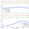 |
Fig. 6 Horizontally and time-averaged (over the final three days of simulation) magnetic pressure (in cgs units) for models with radial (top) and horizontal (bottom) magnetic field plotted as a function of radiation temperature. There is a nearly constant pressure for the strong magnetic field models, whereas the moderately strong models experience decompression near the base and compression around the iron opacity bump, mimicking piston-like dynamics for our numerical models. |
4 Discussion
In the previous section we illustrate how strong magnetic fields of order ~ 10–20 kG are able to suppress the vigorous turbulent motions generated beneath the surface in O stars (at least in the direction perpendicular to the introduced field); by contrast, fields of strengths of ~1 kG only marginally affect the turbulent motions observed in the simulations, rendering results that are qualitatively similar to those seen in non-magnetic models. These results overall agree well with observations of magnetic O stars, where a large macroturbulence is needed to fit optical absorption lines for all magnetic O stars except NGC 1624-2, lending support to the hypothesis by Sundqvist et al. (2013) (see discussion in Sect. 1).
In a further analysis of these simulation outcomes, Figure 6 presents the magnetic pressure, averaged horizontally and over the final three days of the simulation, for models with radial (top panel) and horizontal (bottom panel) magnetic field orientations, plotted as a function of the horizontal and time-averaged radiation temperature (which closely aligns with the gas temperature in these optically thick regions). As expected, in the strongest magnetic field cases, the magnetic pressure remains nearly constant throughout the computational domain, reflecting the stabilising influence of a strong field. In contrast, the weaker field case (1 kG) shows decompression near the base and compression near the iron opacity peak, indicative of the piston-like dynamics discussed above.
Furthermore, Figure 7 shows the horizontally and time- averaged ratio of magnetic pressure to gas pressure, defined as
 (16)
(16)
with standard ‘plasma β’. For η > 1 the field thus dominates and gas parcels should be effectively forced to move along the field lines. Vice versa, for η < 1 the gas dominates and field lines should essentially be dragged along with any motions initiated in the atmosphere. We use η here, rather than its inverse β, in order to be consistent with the previous models of magnetic line-driven winds, where the definition of η has also included the kinetic energy of the gas, which is much higher than the gas pressure in line-driven outflows (ud Doula & Owocki 2002). For the subsurface and photospheric regions in focus here, however, the gas pressure is typically higher than this kinetic energy component, especially for strongly magnetic models where the magnetic field can suppress bulk plasma motions significantly.
Figure 7 then shows explicitly how in the 1 kG simulation η < 1 for the whole sub-photospheric atmosphere, meaning that any gas motions initiated in these regions should be only marginally affected by the presence of the field. We note, however, that also for this case η increases to above unity in the line-driven wind parts above the photosphere, in agreement with previous magnetic line-driven wind simulations starting from a static and smooth stellar surface (ud Doula & Owocki 2002). For the 10 and 20 kG simulations, on the other hand, η remains above unity even well below the visible stellar surface. In the figure we can see that η crosses unity at T ≈ 170–190 kK for the 10 kG cases and at T ≈ 230–250 kK for the 20 kG cases. Since atmospheric turbulence is generated in the iron opacity bump layers around T ~ 150–200 kK, this gives a direct explanation to the low RMS atmospheric velocities found in the previous section for the strong field cases.
Figure 8 next shows the horizontal- and time-averaged ratio of magnetic pressure to the total pressure that now includes radiation pressure (i.e. ηrad ≡ PB/(Pgas + prad)), as done in MacDonald & Petit (2019). Clearly, ηrad < 1 near the iron opacity peak for even the strongest magnetic field cases, yet they fully suppress the atmospheric velocity fluctuations. This suggests that the interplay between the gas pressure and magnetic pressure is indeed the principal factor in the suppression of turbulent motions here.
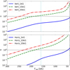 |
Fig. 7 Horizontally and time-averaged (over the final three days of simulation) ratio of magnetic to gas pressure (η = PB/pgas) for models with radial (top) and horizontal (bottom) magnetic field plotted as a function of radiation temperature. The range has been adjusted to highlight the sub-surface region near the iron opacity bump (dotted vertical line) extending to the photosphere where a stellar wind is launched. |
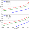 |
Fig. 8 Same as Figure 7, but including radiation pressure in the definition ηrad ≡ PB/(pgas + prad). It shows that ηrad remains below unity near iron opacity peak even for the strongest magnetic case. Even so, these models suppress atmospheric velocity fluctuations, suggesting that pgas plays the key role in this phenomenon. |
4.1 Analytic scaling relation for magnetic suppression of atmospheric turbulence
We can further understand these results through the approximate scaling relation provided by Sundqvist et al. (2013). The temperature T0 at which gas pressure equals magnetic pressure (i.e. the temperature at which η = 1), was estimated using a simple grey atmosphere in hydrostatic equilibrium, yielding (their Eq. (3))
 (17)
(17)
where  is an average opacity for the sub-surface atmosphere, geff is the effective gravity (reduced by radiative acceleration), and it has been assumed that the optical depth τ ≫ 1 at T02. Assuming opacity dominated by electron scattering (approximately true below the critical iron opacity region), for Teff = 40 kK and geff = 4050 we obtain T0 ≈ 50 kK for B = 1 kG, T0 ≈ 160 kK for B = 10 kG, and T0 ≈ 230 kK for B = 20 kG. These characteristic analytic estimates compare reasonably well with the detailed simulation results above, as do similar estimates of critical field strengths above which the magnetic field can suppress turbulence by MacDonald & Petit (2019) and Jermyn & Cantiello (2020). In those studies, however, the kinetic energy of the turbulent gas was estimated by simple mixing length theory (MLT) for convection, whereas our O star simulations (here and in Debnath et al. 2024) show that such MLT cannot be used to estimate turbulent velocities arising from instabilities in the sub-surface iron-bump region of O stars. As such, Eq. (17) above provides a straightforward simple rationale for understanding how potential suppression of photospheric turbulence by the magnetic field scales with basic atmospheric parameters.
4.2 Magnetically induced atmospheric inflation of luminous massive stars
As shown in Table 2 and Figure 3, the size of the photosphere, Rphot, depends not only on the magnetic field strength, but also strongly on its orientation. For models with a radial magnetic field, Rphot fluctuates (because of the oscillatory motions discussed above), but its average value remains only marginally affected, regardless of the field strength. However, for models with a strong horizontal magnetic field, a significant increase in Rphot is observed in the simulations.
This inflation effect very likely occurs in the models precisely because turbulent motions are suppressed; indeed, it mimics the inflationary behaviour seen in 1D models of luminous massive stars assuming a radiative stellar envelope in hydrostatic equilibrium (see e.g. discussions in Petrovic et al. 2006; Gräfener et al. 2012; Poniatowski et al. 2021; Debnath et al. 2024); the key physics driving this mechanism is the higher opacity in the iron-bump region, which pushes the luminous star towards its effective Eddington limit. The only way the envelope can then remain in hydrostatic balance is by expansion of its envelope and atmosphere. Since radiative luminosity is conserved, the larger radius then also leads to a lower stellar effective temperature, as seen in Table 2. We note that this inflation effect thus generally becomes more prominent the closer the radiative massive star is to the classical Eddington limit (see also discussion in Owocki 2015).
This tentatively suggests that the observable surface of luminous massive stars with strong global dipole fields could be significantly asymmetric and deformed, where an observer viewing from the magnetic equator might see a significantly larger and less variable star than an observer viewing from above the magnetic pole. It is important to note, however, that our local 2D simulations neglect potentially important global transport effects. For example, if rapid lateral diffusion of photons were able to equilibrate polar and equatorial regions, this could significantly reduce the pronounced latitudinal effects on stellar temperature and radius found here.
4.3 Inefficient convective instability in iron opacity peak region of O stars
The very turbulent O-star atmospheres seen in the RHD simulations by Jiang et al. (2015) and Debnath et al. (2024) have normally been interpreted in terms of sub-surface convection arising in the iron opacity peak region. However, as mentioned above (see also discussions in Jiang et al. 2015 and Debnath et al. 2024) energy transport by enthalpy (i.e. by convection) is actually very inefficient in this region. Detailed linear stability analysis (Blaes & Socrates 2003; van der Sijpt et al., in prep.) demonstrates that more instabilities are present in the region (e.g. radiatively driven unstable sound waves and classical Rayleigh- Taylor instabilities), and that structure growth may instead be dominated by these. This is supported by the simulations here, especially the strong 20 kG vertical field case. Specifically, linear stability analysis including magnetic fields (Blaes & Socrates 2003) shows that a strong vertical field that suppresses horizontal motion will also be able to completely suppress convection (simply because there is no gravity mode instability in the vertical direction). A similar reasoning was also used in MacDonald & Petit (2019) to argue that a strong vertical field should stabilise the atmosphere against convection, while an equally strong horizontal field should not (see their Sect. 2.2).
This is in stark contrast to our 2D RMHD model results, where large radial motions still occur in the simulations with a strong vertical field; that is, the atmospheric motions in those simulations cannot stem from the convective instability. Instead, they very likely arise because the effective Eddington limit is exceeded already at the sub-surface iron opacity peak, launching failed wind outflows that stagnate and start to fall back as the opacity decreases when approaching the optical surface. Since the outward suction effect from line-driving is efficient only near and above this surface, and the gas is prevented by the magnetic field from moving horizontally, the outcome is a radially oscillating atmosphere characterised by alternating infalling and outflowing regions. In contrast, in the simulations with a strong horizontal field, this radial motion is effectively suppressed, leading instead to a quasi-hydrostatic atmosphere, and thereby to the inflation effect discussed above. Since curvature effects will break the symmetries of the local 2D simulations presented here, it is likely that (if real) these radial atmospheric motions would be constrained to regions close to the magnetic pole.
5 Summary and future work
The work here has provided new insights into the role of strong magnetic fields in suppressing velocity fluctuations within the sub-surface layers of O stars, particularly in those with magnetic fields exceeding 10 kG in horizontal direction. Our 2D RMHD simulations reveal that such strong magnetic fields can effectively suppress the large turbulent motions typically associated with the atmospheres of these stars. This finding offers a plausible explanation for the unique case of NGC 1624-2, which possesses a very strong ~20 kG dipolar field and does not exhibit the additional line-broadening (macroturbulence) observed in the optical absorption lines of other magnetic and non-magnetic O stars (Sundqvist et al. 2013). Analogously, this suppression also means that if significant stochastic low-frequency variability (e.g. Bowman et al. 2024) were to be found in NGC 1624-2, it would speak against an origin of such low-frequency variability in the sub-surface turbulent region of massive stars (see also discussion in Jermyn & Cantiello 2020).
In models with radial magnetic field orientation, the stellar surface exhibits piston-like oscillations, a signature of vertical motion induced by the field-aligned configuration. These oscillations are characterised by periodic compression and expansion of the gas, which is able to flow freely along the radial magnetic field lines. The motion occurs on a timescale of about half a day, quite similar to the oscillatory behaviour found in the simulations by Jiang et al. (2017) for cases with weaker fields up to 1 kG. As discussed above, since there is no gravity mode instability in the radial direction this also shows that it is not convection that primarily drives these atmospheric motions.
On the other hand, in models with a strong horizontal magnetic field, these piston-like motions are significantly suppressed. The horizontal field orientation effectively inhibits the radial movement of gas, likely due to the magnetic tension forces acting to resist vertical displacement. Instead of oscillating, the gas remains relatively stationary, suggesting that the magnetic field in this configuration is able to fully constrain the large velocity fluctuations that would otherwise occur. This stark difference between the radial and horizontal magnetic configurations highlights the importance of magnetic field geometry in governing the dynamics of the atmospheres of magnetic massive stars. In particular, strong horizontal fields appear to almost completely quench the instabilities driving turbulence in massive-star envelopes, leading to a more stable atmosphere.
As discussed in the previous section, this quenching also leads to significant envelope inflation in the simulations with strong horizontal magnetic fields. By contrast, an equally strong radial field shows a fluctuating photosphere, but with an average value that is only marginally different from the non-magnetic simulations. This may suggest that in luminous massive stars with strong global dipole fields, the observable surface above the magnetic equator might be significantly larger, cooler, and less variable than the surface above the magnetic pole.
While these results are promising and seem to offer a natural explanation for the broad characteristics of observed optical absorption lines in magnetic O stars, it is important to keep in mind that they are based on 2D local simulations, which inherently limit the ability to capture the full complexity of the stellar atmospheres. Full global 3D RMHD simulations including curvature effects will indeed be needed to confirm the presence of the radial piston-like motions above the pole as well as the potential atmospheric inflation above the magnetic equator discussed above. In particular, rapid lateral photon diffusion may induce a more uniform thermal structure in latitude than found in the local simulations here and might also affect the strength of vertical motions in polar regions. Future work should thus focus on extending these simulations to full 3D global models including curvature effects and the spherical divergence of the magnetic field. Such an approach would allow for a more consistent and systematic investigation of atmospheric turbulence suppression. This would also be required for a more quantitative analysis of the narrow absorption lines observed for NGC 1624-2 (Wade et al. 2012b; David-Uraz et al. 2021), since the observer’s viewing angle and the global magnetic field topology will both affect the surface-integrated spectral line formation.
In conclusion, our work here provides a foundation for such future studies aiming to further explore the intricate interplay between magnetic fields and atmospheric turbulence in O stars. Such studies are essential for a deeper understanding of the variability observed in the spectra of magnetic massive stars and the role of magnetic fields in shaping their atmospheres.
Acknowledgements
We are grateful to Stan Owocki for providing fruitful suggestions in performing this study. A.u.-D. acknowledges NASA ATP grant number 80NSSC22K0628 and support by NASA through Chandra Award number TM4-25001A issued by the Chandra X-ray Observatory 27 Center, which is operated by the Smithsonian Astrophysical Observatory for and on behalf of NASA under contract NAS8-03060. The computational resources used for this work were provided by the Penn State University Collab Roar system. D.D., N.M., and J.S. acknowledge the support of the European Research Council (ERC) Horizon Europe under grant agreement number 101044048 (ERC-2021-COG, SUPERSTARS-3D). J.S. and A.u.-D. acknowledge support from the Belgian Research Foundation Flanders (FWO) Odysseus program under grant number G0H9218N. JS further acknowledges support from FWO grant G077822N. RK is supported by FWO projects G0B4521N and G0B9923N and received funding from the European Research Council (ERC) under the European Union Horizon 2020 research and innovation program (grant agreement No. 833251 PROMINENT ERC-ADG 2018). We gratefully thank our referee, Matteo Cantiello, for useful suggestions that helped us add some important nuances to the discussion of our results. Finally, the authors would like to thank all members of the KUL-EQUATION group for fruitful discussion, comments, and suggestions We made significant use of the following packages to analyze our data: NumPy (Harris et al. 2020), SciPy (Virtanen et al. 2020), matplotlib (Hunter 2007), Python amrvac_reader (Keppens et al. 2020).
References
- Blaes, O., & Socrates, A. 2003, ApJ, 596, 509 [CrossRef] [Google Scholar]
- Bowman, D. M., Van Daele, P., Michielsen, M., & Van Reeth, T. 2024, A&A, 692, A49 [NASA ADS] [CrossRef] [EDP Sciences] [Google Scholar]
- Cantiello, M., Langer, N., Brott, I., et al. 2009, A&A, 499, 279 [NASA ADS] [CrossRef] [EDP Sciences] [Google Scholar]
- Castor, J. I., Abbott, D. C., & Klein, R. I. 1975, ApJ, 195, 157 [Google Scholar]
- Conti, P. S., & Ebbets, D. 1977, ApJ, 213, 438 [CrossRef] [Google Scholar]
- David-Uraz, A., Petit, V., Shultz, M. E., et al. 2021, MNRAS, 501, 2677 [NASA ADS] [CrossRef] [Google Scholar]
- Debnath, D., Sundqvist, J. O., Moens, N., et al. 2024, A&A, 684, A177 [NASA ADS] [CrossRef] [EDP Sciences] [Google Scholar]
- Gräfener, G., Owocki, S. P., & Vink, J. S. 2012, A&A, 538, A40 [NASA ADS] [CrossRef] [EDP Sciences] [Google Scholar]
- Grassitelli, L., Fossati, L., Simón-Diáz, S., et al. 2015, ApJ, 808, L31 [NASA ADS] [CrossRef] [Google Scholar]
- Grunhut, J. H., Wade, G. A., Neiner, C., et al. 2017, MNRAS, 465, 2432 [NASA ADS] [CrossRef] [Google Scholar]
- Harris, C. R., Millman, K. J., van der Walt, S. J., et al. 2020, Nature, 585, 357 [NASA ADS] [CrossRef] [Google Scholar]
- Howarth, I. D., Siebert, K. W., Hussain, G. A. J., & Prinja, R. K. 1997, MNRAS, 284, 265 [NASA ADS] [CrossRef] [Google Scholar]
- Hunter, J. D. 2007, Comput. Sci. Eng., 9, 90 [NASA ADS] [CrossRef] [Google Scholar]
- Jermyn, A. S., & Cantiello, M. 2020, ApJ, 900, 113 [NASA ADS] [CrossRef] [Google Scholar]
- Jiang, Y.-F., Cantiello, M., Bildsten, L., Quataert, E., & Blaes, O. 2015, ApJ, 813, 74 [Google Scholar]
- Jiang, Y.-F., Cantiello, M., Bildsten, L., Quataert, E., & Blaes, O. 2017, ApJ, 843, 68 [NASA ADS] [CrossRef] [Google Scholar]
- Keppens, R., Meliani, Z., van Marle, A. J., et al. 2012, J. Comput. Phys., 231, 718 [Google Scholar]
- Keppens, R., Teunissen, J., Xia, C., & Porth, O. 2020, arXiv e-prints [arXiv:2004.03275] [Google Scholar]
- Keppens, R., Braileanu, B. P., Zhou, Y., et al. 2023, A&A, 673, A66 [NASA ADS] [CrossRef] [EDP Sciences] [Google Scholar]
- Landstreet, J. D. 1998, A&A, 338, 1041 [NASA ADS] [Google Scholar]
- Levermore, C., & Pomraning, G. 1981, ApJ, 248, 321 [NASA ADS] [CrossRef] [Google Scholar]
- MacDonald, J., & Petit, V. 2019, MNRAS, 487, 3904 [NASA ADS] [CrossRef] [Google Scholar]
- Michaud, G. 1970, ApJ, 160, 641 [Google Scholar]
- Moens, N., Poniatowski, L. G., Hennicker, L., et al. 2022, A&A, 665, A42 [NASA ADS] [CrossRef] [EDP Sciences] [Google Scholar]
- Moens, N., Sundqvist, J., El Mellah, I., et al. 2022, A&A, 657, A81 [NASA ADS] [CrossRef] [EDP Sciences] [Google Scholar]
- Narechania, N., Keppens, R., ud Doula, A., et al. 2024, A&A, submitted [Google Scholar]
- Owocki, S. P. 2015, in Very Massive Stars in the Local Universe, ed. J. S. Vink, Astrophys. Space Sci. Libr., 412, 113 [NASA ADS] [CrossRef] [Google Scholar]
- Pauldrach, A., Puls, J., & Kudritzki, R. P. 1986, A&A, 164, 86 [NASA ADS] [Google Scholar]
- Petrovic, J., Pols, O., & Langer, N. 2006, A&A, 450, 219 [NASA ADS] [CrossRef] [EDP Sciences] [Google Scholar]
- Poniatowski, L. G., Sundqvist, J. O., Kee, N. D., et al. 2021, A&A, 647, A151 [NASA ADS] [CrossRef] [EDP Sciences] [Google Scholar]
- Poniatowski, L. G., Kee, N. D., Sundqvist, J. O., et al. 2022, A&A, 667, A113 [NASA ADS] [CrossRef] [EDP Sciences] [Google Scholar]
- Porth, O., Xia, C., Hendrix, T., Moschou, S., & Keppens, R. 2014, ApJS, 214, 4 [NASA ADS] [CrossRef] [Google Scholar]
- Powell, K. G. 1994, An approximate Riemann solver for magnetohydrodynamics (that works in more than one dimension), Tech. rep. [Google Scholar]
- Puls, J., Vink, J. S., & Najarro, F. 2008, A&A Rev., 16, 209 [NASA ADS] [CrossRef] [Google Scholar]
- Rogers, F. J., & Iglesias, C. A. 1992, ApJ, 401, 361 [NASA ADS] [CrossRef] [Google Scholar]
- Sander, A. A. C., Hamann, W. R., Todt, H., Hainich, R., & Shenar, T. 2017, A&A, 603, A86 [NASA ADS] [CrossRef] [EDP Sciences] [Google Scholar]
- Schneider, F. R. N., Ohlmann, S. T., Podsiadlowski, P., et al. 2019, Nature, 574, 211 [Google Scholar]
- Schultz, W. C., Bildsten, L., & Jiang, Y.-F. 2022, ApJ, 924, L11 [NASA ADS] [CrossRef] [Google Scholar]
- Simón-Díaz, S., & Herrero, A. 2007, A&A, 468, 1063 [NASA ADS] [CrossRef] [EDP Sciences] [Google Scholar]
- Simón-Díaz, S., Godart, M., Castro, N., et al. 2017, A&A, 597, A22 [CrossRef] [EDP Sciences] [Google Scholar]
- Sundqvist, J. O., Petit, V., Owocki, S. P., et al. 2013, MNRAS, 433, 2497 [NASA ADS] [CrossRef] [Google Scholar]
- Sundqvist, J. O., Björklund, R., Puls, J., & Najarro, F. 2019, A&A, 632, A126 [NASA ADS] [CrossRef] [EDP Sciences] [Google Scholar]
- Turner, N. J., & Stone, J. M. 2001, ApJS, 135, 95 [NASA ADS] [CrossRef] [Google Scholar]
- ud Doula, A., & Owocki, S. P. 2002, ApJ, 576, 413 [NASA ADS] [CrossRef] [Google Scholar]
- Ud-Doula, A., Owocki, S. P., & Townsend, R. H. D. 2009, MNRAS, 392, 1022 [Google Scholar]
- Virtanen, P., Gommers, R., Oliphant, T. E., et al. 2020, Nature Methods, 17, 261 [CrossRef] [Google Scholar]
- Wade, G. A., Grunhut, J. H., & MiMeS Collaboration 2012a, in Circumstellar Dynamics at High Resolution, eds. A. C. Carciofi, & T. Rivinius, ASP Conf. Ser., 464, 405 [Google Scholar]
- Wade, G. A., Maíz Apellániz, J., Martins, F., et al. 2012b, MNRAS, 425, 1278 [NASA ADS] [CrossRef] [Google Scholar]
- Xia, C., Teunissen, J., Mellah, I. E., Chané, E., & Keppens, R. 2018, ApJS, 234, 30 [NASA ADS] [CrossRef] [Google Scholar]
There is a slight inconsistency in our approach: while all hydrodynamical quantities incorporate spherical divergence, the evolution of the magnetic field does not. Given that the range of our computational domain is relatively small, we do not expect our results and conclusions to change qualitatively.
The original scaling used the actual stellar gravity rather than that reduced by radiative acceleration (see also comments by MacDonald & Petit 2019), but in practice this does not change the overall scaling results because of the relatively weak g−1/4 dependence.
All Tables
Horizontally time-averaged values of Rphot, Teff, log(g), and T0 (estimated temperature where magnetic and gas pressure are equal to each other) for all the models in this study.
All Figures
|
Fig. 1 Illustrative temporal evolution of a magnetic model with a 1 kG radial magnetic field. The colour scale represents the logarithm of density in cgs units, while the blue lines depict the magnetic field lines. Beginning with a spherically symmetric initial condition (left panel) threaded by a uniform magnetic field in radial direction, the model develops significant density and velocity variations after two to four days (middle panel; time = 3 d) and maintains them until the end of the simulation at approximately nine days (right panel; time = 6 d). |
| In the text | |
|
Fig. 2 Similar to Fig. 1, but comparing the late evolutionary states between the non-magnetic case (left column) and various magnetic models. The second column from the right shows models with a 1 kG magnetic field in the radial (top row) and horizontal (bottom row) directions. The third and fourth columns display models with 10 kG and 20 kG magnetic fields, respectively. |
| In the text | |
|
Fig. 3 Horizontally averaged density profiles as a function of time, using the modified radial coordinate x (≡ r − R0/r). The leftmost column serves as a non-magnetic reference. The top row displays models with radial magnetic fields of 1, 10, and 20 kG, while the bottom row shows models with horizontal magnetic fields of the same strengths. The dotted black line indicates the photospheric radius (r(τ = 2/3)), and the solid black line marks the location of the iron opacity peak (T ~ 1.6e5 K). |
| In the text | |
|
Fig. 4 Horizontally averaged radial velocity vr plotted as modified radial coordinate x (≡ r − R0/r) vs. time. The leftmost column represents the non-magnetic case for a direct comparison. The top row shows models with a radial magnetic field of 1, 10, and 20 kG. Similarly, the bottom panels show models with a horizontal magnetic field of 1, 10, and 20 kG. The dotted black line represents the photospheric radius (Rphot ≡ r(τ = 2/3) and the solid black line denotes the location of the iron opacity peak (T ~ 1.6 × 10⁵ K). The radial magnetic field does not inhibit up-and-down piston-like motions of the gas, whereas the strong horizontal magnetic field can fully suppress it. This figure also demonstrates clearly how velocity dispersion is initiated near the iron opacity peak (solid black line). We show only the final ~3 d of simulation for all models. Coincidentally, the model with 1 kG radial magnetic field was caught in one of the episodes of outbursts, which is also visible in Fig. 3, albeit less prominently. |
| In the text | |
|
Fig. 5 Root mean square (RMS) values of radial (top panels) and tangential velocity perturbations (bottom panels) are shown for selected magnetic models as a function of radiation temperature, focusing on the (sub-)surface atmospheric layers before the onset of the stellar wind. The left column illustrates the results for a radial magnetic field configuration, while the right column corresponds to a horizontal magnetic field configuration. It is evident that a strong radial magnetic field suppresses horizontal gas motion, while a strong horizontal magnetic field inhibits radial gas movement. Notably, in the strongest field cases (20 kG), the tangential velocity perturbations approach or fall below 1 km/s. |
| In the text | |
|
Fig. 6 Horizontally and time-averaged (over the final three days of simulation) magnetic pressure (in cgs units) for models with radial (top) and horizontal (bottom) magnetic field plotted as a function of radiation temperature. There is a nearly constant pressure for the strong magnetic field models, whereas the moderately strong models experience decompression near the base and compression around the iron opacity bump, mimicking piston-like dynamics for our numerical models. |
| In the text | |
|
Fig. 7 Horizontally and time-averaged (over the final three days of simulation) ratio of magnetic to gas pressure (η = PB/pgas) for models with radial (top) and horizontal (bottom) magnetic field plotted as a function of radiation temperature. The range has been adjusted to highlight the sub-surface region near the iron opacity bump (dotted vertical line) extending to the photosphere where a stellar wind is launched. |
| In the text | |
|
Fig. 8 Same as Figure 7, but including radiation pressure in the definition ηrad ≡ PB/(pgas + prad). It shows that ηrad remains below unity near iron opacity peak even for the strongest magnetic case. Even so, these models suppress atmospheric velocity fluctuations, suggesting that pgas plays the key role in this phenomenon. |
| In the text | |
Current usage metrics show cumulative count of Article Views (full-text article views including HTML views, PDF and ePub downloads, according to the available data) and Abstracts Views on Vision4Press platform.
Data correspond to usage on the plateform after 2015. The current usage metrics is available 48-96 hours after online publication and is updated daily on week days.
Initial download of the metrics may take a while.