| Issue |
A&A
Volume 684, April 2024
|
|
|---|---|---|
| Article Number | A7 | |
| Number of page(s) | 15 | |
| Section | Stellar atmospheres | |
| DOI | https://doi.org/10.1051/0004-6361/202347015 | |
| Published online | 29 March 2024 | |
Simulating small-scale dynamo action in cool main-sequence stars
1
Istituto ricerche solari Aldo e Cele Daccò (IRSOL), Faculty of Informatics, Università della Svizzera italiana, 6605 Locarno, Switzerland
2
Euler Institute, Università della Svizzera italiana (USI), 6900 Lugano, Switzerland
e-mail: This email address is being protected from spambots. You need JavaScript enabled to view it.
3
Leibniz-Institut für Sonnenphysik (KIS), Schöneckstrasse 6, 79104 Freiburg im Breisgau, Germany
4
Theoretical Astrophysics, Department of Physics and Astronomy, Uppsala University, Box 516, 751 20 Uppsala, Sweden
Received:
26
May
2023
Accepted:
1
December
2023
Abstract
Context. The origin of the ubiquitous small-scale magnetic field observed on the solar surface can be attributed to the presence of a small-scale dynamo (SSD) operating in the sub-surface layers of the Sun. It is expected that a similar process could self-sustain a considerable amount of magnetic energy also in the near-surface layers of cool main-sequence stars other than the Sun.
Aims. In this paper the properties of the magnetic field resulting from SSD action operating in the near-surface layers of four cool main-sequence stars and its self-organization into magnetic flux concentrations are investigated numerically.
Methods. Three-dimensional radiative magnetohydrodynamic simulations of SSD action in the near-surface layers of four cool main-sequence stars of spectral types K8V, K2V, G2V, and F5V are carried out with the CO5BOLD code. The simulations are set up to have approximately the same Reynolds and magnetic Reynolds numbers, and to disentangle the impact of the effective temperature and the surface gravity on the SSD action from numerical effects.
Results. It is found that the SSD growth rates in SI units differ for the four stellar models; the highest and lowest growth rate is for the K2V and F5V model, respectively. This is due to the different turnover times in the four simulations. Even so, the SSD field strengths reached in the saturation phases are similar in all models, with the same amount of kinetic energy converted into magnetic energy. If the magnetic energy that is pumped out from the computational domain across the bottom boundary is partially replenished from outside of the computational domain, we find that the SSD action leads to a sufficient reduction in the convective velocities to reduce the convective horizontal length scales in the convection zone by 5–10%, vanishing towards the optical depth unity level. In this case, strong kilogauss magnetic flux concentrations emerge at the surface, leading to magnetic bright features, which are more numerous and conspicuous for the K2V and G2V models than for the K8V and F5V models. Their vertical magnetic field component on the surface of optical depth unity increases from 1 kG to 1.6 kG with decreasing effective temperature from F5V to K8V. However, more than 90% of the magnetic flux through any of these stellar surfaces has a field strength of less than 1 kG.
Key words: dynamo / magnetohydrodynamics (MHD) / turbulence / methods: numerical / stars: atmospheres / stars: magnetic field
© The Authors 2024
 Open Access article, published by EDP Sciences, under the terms of the Creative Commons Attribution License (https://creativecommons.org/licenses/by/4.0), which permits unrestricted use, distribution, and reproduction in any medium, provided the original work is properly cited.
This article is published in open access under the Subscribe to Open model. This email address is being protected from spambots. You need JavaScript enabled to view it. to support open access publication.
1 Introduction
Spectropolarimetric observations show that the atmospheres of cool main-sequence stars are permeated by magnetic fields covering a wide range of spatio-temporal scales (for reviews, see e.g. Donati & Landstreet 2009; Reiners 2012; Kochukhov et al. 2017 and references therein). The surface of the Sun, the most studied cool main-sequence star, is covered by magnetic fields on spatial scales ranging from the 30 000 km of super-granular cells down to the smallest magnetic features resolvable with current instruments on scales of less than 100 km (see e.g. Solanki et al. 2006; Wedemeyer-Böhm et al. 2009; Fan 2021). The interaction of such magnetic fields with atmospheric plasma flows plays a crucial role in determining the dynamics of particles and heat transfer near the solar surface and the photometric and spectral variability of the Sun. For example, large-scale magnetic fields are responsible for the emergence of dark sunspots, whereas small-scale magnetic flux concentrations appear as bright features. Evidence of magnetic activity leading to the formation of Sun-like spots has also been found for stars other than the Sun (see e.g. Berdyugina 2005; Strassmeier 2009). However, because of the lack of high-resolution observations for cool main-sequence stars other than the Sun, very little is known about magnetic fields on scales much smaller than the radius of these stars. This is a critical issue not only in the context of stellar physics, but also for exoplanet detection. Transit observations, and in particular transmission spectroscopy, the technique used to determine the atmospheric composition of an exoplanet, rely on a precise understanding of the wavelength-dependent brightness fluctuations of the star being occulted. This, in turn, requires a detailed modelling of the magnetic fields and of the turbulent plasma flows present in the proximity of the stellar surface (Rackham et al. 2023).
High-resolution observations of the Sun suggest that small-scale magnetic activity is ubiquitous on the solar surface, and that the magnetic flux in internetwork regions is independent of the solar cycle (Ramelli et al. 2019). A widely accepted explanation for this behaviour is the presence of a small-scale dynamo (SSD) operating in the sub-surface layers of the Sun. In the recent past, radiative magnetohydrodynamic (MHD) numerical simulations have provided many insights into the functioning of the sub-surface solar SSD, showing that a considerable amount of magnetic energy in the solar photosphere could be self-sustained through dynamo action (see e.g. Cattaneo 1999; Vögler & Schüssler 2007; Pietarila Graham et al. 2010; Rempel 2014; Kitiashvili et al. 2015; Thaler & Spruit 2015; Khomenko et al. 2017). On the other hand, numerical studies of small-scale magnetic fields on the surface of cool main-sequence stars other than the Sun mostly focus on how the magnetic field self-organizes and affects the surrounding plasma, neglecting how the magnetic field was initially produced. Seminal work in this respect was done by Beeck and collaborators in 2011, further extended in 2015, who found a substantial variation in the properties of the surface magneto-convection between main-sequence stars of different spectral types as a consequence of including magnetic fields in the simulations (Beeck et al. 2011, 2015). Additional work in this context was done by Steiner and collaborators, who analysed MHD models of spectral types K8V to F5V, showing that the field strength of the strongest flux concentrations was fairly independent of spectral type when measured at the optical depth level τR = 1 (Steiner et al. 2014). This work was then extended by Salhab et al. (2018), who found that small-scale magnetism increases the bolometric intensity and flux in all the investigated models, most prominently for the Sun.
The possibility of simulating SSD action on stars other than the Sun has been investigated only very recently. In Bhatia et al. (2022), the authors discuss how small-scale magnetic fields generated by SSD action on the surface of different cool main-sequence stars introduce small but significant changes in thermodynamic stratification due to a reduction in the convective velocities. In a second publication of the series, it is shown how the SSD is affected by the metallicity of the stellar plasma (Witzke et al. 2023). These works provided a first insight into the functioning of SSDs on the surface of stars other than the Sun, but a number of questions related to SSD action in the atmosphere of cool main-sequence stars still remains. This motivates the present work.
In this paper we present simulations and their analysis of the same spectral sequence, that is same effective temperatures and solar metallicity, that was considered in the work of Salhab et al. (2018), which are K8V, K2V, G2V, and F5V, but with a surface gravity more consistent with stars on the main sequence. All simulations were carried out with the CO5BOLD code (Freytag et al. 2012), starting from a relaxed non-magnetic state, to which we add a small magnetic field seed, which then is evolved until saturation of the magnetic energy. The aims of our work are (i) to investigate the differences in SSD action among the four models during the kinematic phase; (ii) to study the properties of magnetic fields amplified by SSD action and how they affect the plasma; and (iii) to examine the properties of surface magnetic flux concentrations that originate from the self-organization of magnetic fields produced by SSD action (the magnetic filigree). In Sect. 2, we present the simulation set-up and the parameters used for the computations. Then, in Sect. 3 we provide a general overview of the simulation results. Section 4 discusses the numerical results for the kinematic phase, during which the magnetic field is amplified exponentially in time. The results obtained after saturation of the magnetic energy are discussed in Sect. 5. Finally, in Sect. 6 we report our conclusions. In Appendix A the results of the simulations are discussed in normalized units, whereas the algorithm used to identify magnetic bright features (MBFs) is presented in Appendix B.
2 Methods and stellar models
The simulations discussed in the present paper were carried out with the CO5BOLD code using the ‘box-in-a-star’ set-up. This corresponds to simulating a small partial volume near the optical surface of a star, encompassing the layers where energy transport changes from predominantly convective to purely radiative. We considered four different cool stellar models, as discussed in the following.
2.1 The CO5BOLD model and implementation
The CO5BOLD code is a numerical tool designed to simulate solar and stellar atmospheres, as well as their interiors, by solving the time-dependent ideal MHD equations, in cgs units,
 (1)
(1)
![Mathematical equation: ${{\partial \rho {\bf{v}}} \over {\partial t}} + \nabla \cdot \left[ {\rho {\bf{vv}} + \left( {P + {{{B^2}} \over {8\pi }}} \right){\bf{I}} - {{{\bf{BB}}} \over {4\pi }}} \right] + \rho \nabla {\rm{\Phi }} = 0,$](/articles/aa/full_html/2024/04/aa47015-23/aa47015-23-eq2.png) (2)
(2)
 (3)
(3)
![Mathematical equation: ${{\partial \rho {e_{{\rm{tot}}}}} \over {\partial t}} + \nabla \cdot \left[ {\left( {\rho {e_{{\rm{tot}}}} + P + {{{B^2}} \over {8\pi }}} \right){\bf{v}} - {1 \over {4\pi }}({\bf{v}} \cdot {\bf{B}}){\bf{B}} + {{\bf{F}}_{{\rm{rad}}}}} \right] = 0,$](/articles/aa/full_html/2024/04/aa47015-23/aa47015-23-eq4.png) (4)
(4)
in combination with an equation of state (eos), used to relate the mass density ρ and the gas pressure P to the internal energy ei, and a non-grey radiative transfer equation. Here v is the plasma velocity, B the magnetic field, ρetot = ρei + ρυ2/2 + B2/(8π) + ρΦ the total energy, Φ the gravitational potential, Frad the frequency-integrated radiative energy flux vector, I the identity matrix, and a⋅b and ab are the scalar and tensor products of vector a with vector b, respectively. The code can be used to carry out both global (star-in-a-box) and local (box-in-a-star) simulations. In the following, only box-in-a-star simulations are considered.
Equations (1)–(4) are evolved using flux-conserving Riemann-type solvers. While a Harten-Lax-van Leer (HLL) solver (Harten et al. 1983) must be used for magnetic simulations, a Roe solver (Roe 1986) can be used as a less diffusive alternative for the non-magnetic case. In regions of low plasma-β, with β the ratio of thermal to magnetic pressure, the equation of the thermal energy is used instead of the equation of the total energy to avoid negative gas pressures, this at the expense of strict energy conservation. The Alfvén speed, υA, can be limited by artificially reducing the strength of the Lorentz force to avoid very small time steps. Moreover, to impose ∇⋅B = 0, the constrained-transport method of Evans & Hawley (1988) is used. Pre-tabulated values as a function of density and internal energy, accounting for the ionisation balance of hydrogen, helium, and a representative metal, are used to solve the eos and to compute the plasma pressure and temperature. To solve the radiative transfer equation, either a short- or a long-characteristic scheme can be used. Opacities are obtained from opacity tables computed using the opacity binning technique, for which spectral lines of similar strength are grouped in bands, and average opacities are computed for each band (Nordlund 1982; Ludwig 1992; Freytag et al. 2012). Additionally, to reduce the computational cost of a simulation, the diffusion approximation can be used to model the radiative transport in the deep, optically thick layers of the numerical domain. The code is written in a modular form using the language Fortran 90 (and some Fortran 77). It is parallelised using a hybrid Message Passing Interface (MPI) and OpenMP parallelization. For more details on CO5BOLD, we refer to Freytag et al. (2012).
For the present paper we used the HLL solver in combination with a second-order reconstruction scheme (of FRweno type; see Freytag 2013). The gravitational field, g = −∇Φ, was assumed vertical and constant. The thermal energy equation was activated for β < 0.1 and υA was limited to a maximum of 50 km s−1. The equations were then evolved in time with a Hancock predictor step. Moreover, we solved the radiative transfer equation with the long-characteristic radiation transport module, using Rosseland mean opacities (grey opacity) and employing the diffusion approximation for depths with min(τR) > 100, where the minimum was evaluated over horizontal planes at constant geometrical height. The Rosseland mean opacities entering the opacity tables were adapted from the MARCS stellar atmosphere package (Gustafsson et al. 2008).
2.2 Stellar parameters
The main governing parameters in these simulations are the effective temperature, Teff; the gravitational acceleration, g; and the chemical composition. Solar metallicity is used for all models. For the effective temperatures, we chose to approximately replicate the nominal temperatures of the four models in Salhab et al. (2018), that is Teff = 4000 K (K8V), 5000 K (K2V), 5770 K (G2V), and 6500 K (F5V). Given these parameters, we used the PARSEC code (Nguyen et al. 2022) to generate two different isochrones, considering 2.0 Gy and 4.6 Gy old stars. The first isochrone was then used to estimate the surface gravity of the F5V model (log 𝑔 = 4.24), whereas the second isochrone was used for the K models (log 𝑔 = 4.66 and log 𝑔 = 4.59 for K8V and K2V models, respectively). Finally, for the G2V model, we considered the solar surface value, log 𝑔 = 4.44. These parameters are summarized in Table 1, where values of four Gaia benchmark stars are also reported to give an idea of where the present models lie on the Hertzsprung-Russell diagram (first two and last three rows, respectively).
2.3 Numerical set-up
The numerical set-up of the simulations in this paper is similar to that used in Riva & Steiner (2022) for the case dh8. More precisely, we consider a Cartesian computational domain with horizontal extension such that the box widths, Lx = Ly, are approximately six mean granular scales. The vertical extension, Lz, is chosen such that the bottom boundary is at a depth where the entropy of the downflowing plasma approaches the essentially constant entropy flow of the upflowing plasma (cf. Fig. 11 of Salhab et al. 2018), whereas the top boundary is located well above the entropy minimum in the photosphere. The exact physical scales and sizes of the four models are reported in Table 1, which also displays the height extent of the boxes in terms of pressure scale heights, with Nbelow = ln(Pbottom/P0) and Nabove = ln(P0/Ptop) the number of pressure scale heights below and above the optical surface, and P0, Pbottom, and Ptop the horizontal and time-averaged gas pressures at the geometrical height z = 0, at the bottom, and at the top of the domain, respectively. Here, z = 0 denotes the space and time-averaged optical depth surface τr = 1.
The granular size is defined as Lgran ≡ 〈Lint(z = 0, t)〉t, where 〈−〉, denotes time averaging and with
 (5)
(5)
the integral length scale for the turbulent motions, kh the horizontal wave number, and  the vertical velocity spectrum. This definition is motivated by the strong correlation between υz(τR = 1) and the emerging vertical bolometric intensity. The pressure scale height is computed as HP = −〈1/∂z ln(〈P〉z)〉t, with 〈−〉z denoting horizontal averaging computed at constant geometrical height. For all models we consider a uniform grid spacing, ∆x = ∆y = ∆z, and nx × ny × nz = 750 × 750 × nz grid cells, where nx, ny, and nz are the number of grid cells in the horizontal directions x and y and in the vertical direction z, respectively, such that we have approximately the same number of grid cells per granule and per pressure scale height, as detailed in Table 1. This is to guarantee similar Reynolds and magnetic Reynolds numbers, Re and Rem, in the four simulations and, consequently, to disentangle the impact of the numerical set-up from the impact of the stellar parameters when drawing conclusions in the following.
To verify that the flow parameters are similar in the four models, we computed the effective viscosity and magnetic diffusivity, v and η, following the methodology detailed in Riva & Steiner (2022) and we used Re = 〈υrms〉t〈Lint〉t/〈v〉t and Rem = 〈υrms〉t〈Lint〉t/〈η〉t, vertically averaged between ln(〈P〉z,t/P0) = 3 and ln(〈P〉z,t/P0) = 1, which is the region where the drive amplitude of the dynamo is largest, as discussed in Sect. 4. Here υrms is the root mean squared (rms) velocity evaluated at constant geometrical height. The magnetic Prandtl number is defined as Prm = Rem/Re. The results are displayed in Table 2. Although Re and Rem show a mild but nearly monotonic increase from model K8V to F5V, we see that the change in Prm is rather modest, smaller than 25% for the four models.
From the values reported in Table 1, we see that both the granular size and the pressure scale height increase with effective temperature. However, when comparing Lgran and HP(z = 0) to the results reported in Table 1 of Salhab et al. (2018), we see that g has a significant impact on stratification properties and on the size of the granules. Larger gravitational accelerations lead to smaller granules and shallower atmospheres, and vice versa for smaller g. This is an expression of the fact that HP ∝ Teff/g.
We use periodic boundaries in both horizontal directions. The top boundary is open for fluid flows and outward radiation, with the density decreasing exponentially in the boundary (ghost) cells outside the domain, whereas magnetic fields are forced to be vertical. Moreover, we impose ∂tvz = −cs∂zvz and ∂zvh = 0, with cs being the local sound speed and vh the horizontal velocity. At the bottom we set an open boundary condition for fluid variables, enforcing ∂zv = 0, vanishing horizontally averaged vertical mass flux, and a control on the specific entropy of the inflowing material to fine tune the resulting effective temperature. The parameters CsChange = 0.1, CpChange = 0.3, and Clin = Csqrt = 0.003 were used to reduce deviations of the entropy, the pressure, and the vertical velocity from the horizontal means, as detailed in Freytag et al. (2012) and Riva & Steiner (2022). For the magnetic field at the bottom boundary, we set ∂zB = 0 in locations of outflowing plasma, whereas we imposed Bx = CB, By = 0, and ∇ ⋅ B = 0 for locations of inflowing plasma, with CB a constant input value discussed in Sect. 3.1. More details on the boundary conditions used in CO5BOLD are given in Freytag (2017).
All simulations were started from the non-magnetic runs of Salhab et al. (2018). The log g values and grids were adapted to match the parameters displayed in Table 1 and the simulations were evolved for several thousand seconds to damp out fluctuations introduced by the interpolations. A seed magnetic field Bz = 1 mG was then added to these relaxed non-magnetic states. From the resulting initial states, we ran four simulations, one for each model, until saturation of the magnetic energy (first saturation), imposing CB = 0. However, to investigate the impact of the bottom boundary condition on the results, after the first saturation stage we continued the simulations with CB ≠ 0, until reaching another saturated state (second saturation). We consider CB ≠ 0 a less stringent condition that matches reality more closely as it allows for some replenishment of the magnetic energy from outside the computational domain. We note that using CB ≠ 0 implies that the magnetic energy is not produced by SSD action alone, but also by amplification of the magnetic field advected into the domain across the bottom boundary. However, although magnetic energy enters the domain in upflow regions, the magnetic energy leaving the domain in downflow regions overcompensates this contribution, thus ensuring a net Poynting flux leaving the domain at the bottom boundary. A more detailed discussion of the impact of these boundary conditions on the results is given in Sect. 5.
Basic physical and numerical parameters for the four simulation models and close Gaia benchmark stars.
Flow parameters and magnetic energy growth rates for the four stellar models.
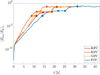 |
Fig. 1 Temporal profiles of magnetic to kinetic energy ratios averaged over the convection zone of the four models K8V, K2V, G2V, and F5V. The round, square, and diamond markers denote phase 1, phase 2, and phase 3, respectively. |
3 Synopsis of the numerical runs
3.1 Evolution
The time-traces of the magnetic to kinetic energy ratio, Em/Ek, are displayed in Fig. 1 for the four models, where 〈−〉c denotes averaging over the convection zone (z < 0). We can identify three main phases. After a few minutes of quick magnetic amplification during which the magnetic flux is expelled from the granules and is transported to the intergranular space, phase 1 starts, in which the magnetic energy is amplified exponentially by the SSD. We consider the end of phase 1 to be the time when 〈Em/Ek〉c = 0.2%, denoted by the round markers in Fig. 1. This low value of 〈Em/Ek〉c corresponds to a still negligible Lorentz-force feedback on the fluid motion. After phase 1, a balance is reached between the amplification of the magnetic field and losses of magnetic energy due to magnetic energy dissipation and to pumping out of the magnetic field across the bottom boundary. Therefore, the simulations reach a statistical steady-state in phase 2 (the first saturated state), whose initial and final points are denoted by the square markers in Fig. 1. Finally, setting CB = 110, 110, 155, and 140 G for models K8V, K2V, G2V, and F5V, respectively, a second saturation state is reached, phase 3, whose initial points are denoted by the diamond markers in Fig. 1. This corresponds to setting  , with
 (6)
(6)
the dynamic equipartition field strength and ρ and vrms evaluated at the bottom of the computational domain. The condition  is motivated by the fact that max(B/Beq dyn) ≃ 8% in the convection zone during phase 2; the maximum value is attained in the deep convection zone, before decreasing to smaller values when approaching the bottom boundary. Therefore, this boundary condition mimics the presence of a SSD operating below the bottom boundary, which generates a magnetic field of strength B ≃ 0.08Beq dyn. We note that the initial points of phases 2 and 3 are determined by eye inspection of the curves displayed in Fig. 1.
Table 3 gives more details on simulation times and output frequencies for each model, with Noutput denoting the number of outputs for the full simulation box (the mass density, internal energy, and velocity and magnetic fields for every grid cell). The emerging vertical bolometric intensity (Ibol), some horizontally averaged quantities, as well as mass density, internal energy, and velocity and magnetic fields at z = 0 were saved every 10 s. Here phase 1 starts at t = 0 and not after the initial expulsion of the magnetic flux from the granules. This is justified by the fact that phase 1 is used in the following as a non-magnetic proxy, and we do not expect the magnetic field to have any noticeable impact on the plasma flow during these first few minutes of the simulations.
Initial and final physical times for each phase and each stellar model and number of time instances of full data output of the entire physical domain used for post-processing.
3.2 Morphology
Figure 2 provides an overview of the basic properties of the simulation results, from the coolest model in the top (K8V) to the warmest in the bottom (F5V). The first three columns display representative time instances of the vertically directed bolometric intensity, normalized to its mean, during phases 1, 2, and 3, respectively; the last column shows the vertical field strength at z = 0 corresponding to the time instances of the third column. The standard picture of bright granules, where the plasma raises to the surface, and dark intergranular lanes, where the plasma flows back into the convection zone, is clearly visible for all models. Moreover, consistent with findings in Beeck et al. (2011), Freytag et al. (2012), and Salhab et al. (2018), among others, the visible continuum intensity contrast of the granular pattern increases from the coolest to warmer models. This increasing intensity contrast with increasing Teff is related to the increase in the relative temperature fluctuations with increasing Teff, as discussed in Beeck et al. (2013) and Salhab et al. (2018), among others. During phase 3 (third column), bright features appear in locations of strong magnetic field. We discuss these features further and the impact that magnetic fields have on plasma flows in Sect. 5.
3.3 Notation
In the following, all the numerical results are evaluated during one of the three main phases discussed above; the initial and final times are reported in Table 3. Uncertainties on the results are computed as the 1σ deviation in temporal fluctuations of the quantities. Horizontal averages are computed either at constant geometrical height (i.e. constant z, denoted in the following as 〈⋅〉z) or over a surface of constant Rosseland opacity (denoted in the following as 〈⋅〉τ). The former is adopted for displaying quantities as a function of height and for analysis in the convection zone, where stratification is nearly adiabatic and largely independent of the radiation field, whereas the latter is favoured for analysis near the optical surface, consistently with the considerations in the Appendix of Beeck et al. (2013). We note that the time t in the index of the angle brackets has the meaning of averaging in time, for example 〈⋅〉zt.
To have a meaningful comparison between models of different spectral types, we used ln(〈P〉z,t/P0) as vertical coordinate instead of z, with the time average of the gas pressure evaluated during the kinematic phase. Quantities on surfaces of constant optical depth were obtained with linear interpolations in ln(τR). To obtain quantities on constant τR we used the full simulation boxes. On the other hand, quantities averaged at constant geometrical height, as well as quantities related to the bolometric intensity, were computed from the data saved each 10 s.
4 Kinematic phase
From Fig. 1, it is clear that the SSD growth rate is different in the four models. By fitting 〈Em/Ek〉c during the kinematic phase with an exponential function, we obtain the energy e-folding times τE ≃ 2700, 2200, 2600, and 3500 s for models K8V, K2V, G2V, and F5V, respectively. These correspond to the magnetic energy growth rates, γE = 1/τE, displayed in the fifth column of Table 2.
To better understand these results, we use the ideal induction equation, Eq. (3), to express the time evolution of the magnetic energy density as
![Mathematical equation: ${\partial _t}{E_{\rm{m}}} = {1 \over {4\pi }}\left[ { - \upsilon \cdot \nabla {{{B^2}} \over 2} + B \cdot (B \cdot \nabla v) - {B^2}\nabla \cdot \upsilon } \right].$](/articles/aa/full_html/2024/04/aa47015-23/aa47015-23-eq10.png) (7)
(7)
Figure 3 displays 〈∂tEm/Em〉t for the four models (solid lines, left axis). This provides an indication of the drive amplitude of the dynamo and where it is most efficient in amplifying the magnetic energy. It results that ∂tEm/Em peaks just beneath the optical surface, at approximately ln(〈P〉z,t/P0) = 2 for all models, with values that are about a factor two higher for the K2V model than for the F5V model. The values for the K8V and G2V models lie between those of the other two models, in agreement with the magnetic energy e-folding times reported above.
The large differences among the four models of the SSD growth rates (with the K2V and F5V models having the lowest and highest γE, respectively) nearly vanish when normalizing the timescales in the system to the turnover time, τ, reported in Table 1. This can be seen from the last column of Table 2, where γEτ is almost independent of the spectral type of the model. More details on the temporal evolution of the models in normalized units are given in Appendix A, where the growth of magnetic to kinetic energy for each model is shown with time units normalized by the corresponding turnover times. Here, we define the turnover time as τ = 1/ maxz(〈vz,rms〉t/〈Lint〉t), where maxz denotes taking the maximum value over the vertical coordinate.
The small variation in γEτ can be understood as follows. It is well known that magnetic energy amplification by SSD is mostly due to the second term on the right-hand side of Eq. (7), B ⋅ (B ⋅ ∇v), called the stretching term, whereas SSD action is suppressed by compression and magnetic diffusivity (see e.g. Batchelor & Taylor 1950). The stretching term is expected to be proportional to the velocity shear term, |∇v|, which is also displayed in Fig. 3 (dashed lines, right axis). Since |∇v| ≈ 1/τ, we have a nearly constant SSD driving term in normalized units.
The impact of compression, which corresponds to the last term of Eq. (7), gets larger when the Mach number, M, of the simulation increases (see e.g. Martins Afonso et al. 2019; Seta & Federrath 2021). At ln(〈P〉z,t/P0) = 2, where the efficiency of the SSD is greatest, we have M = 〈vrms/cs,rms〉t = 0.18, 0.27, 0.34, and 0.48 for models K8V, K2V, G2V, and F5V, respectively, with cs,rms the rms value of the sound speed. Hence, the effect of compression is smallest for K8V and largest for F5V. However, the impact of compression on the SSD operation is marginal for the present models, as discussed in the following, and therefore it is not expected to noticeably affect the value of γEτ. Finally, concerning the effect of magnetic diffusivity, in normalized units one would expect higher growth rates for larger Rem and larger Prm, and vice versa for smaller Rem and smaller Prm (Brandenburg & Subramanian 2005; Käpylä et al. 2018). However, the changes in Rem and in Prm are rather mild (see the third and fourth columns of Table 2). Consequently, γEτ is almost constant in the present models.
Energy transfer analysis. To gain a deeper insight into the mechanism driving SSD action, we performed an energy transfer analysis similar to Pietarila Graham et al. (2010), Rempel (2014), and Riva & Steiner (2022). In particular, we write the spectral magnetic energy as
 (8)
(8)
whose time evolution can be decomposed into the three components
 (9)
(9)
where
 (10)
(10)
 (11)
(11)
 (12)
(12)
are the energy transfers to and from the magnetic energy due to advection, stretching, and compression of the magnetic field, respectively. Here  denotes the Fourier transform, * the complex conjugate, and c.c. the respective complex conjugate expression. A detailed analysis of these terms close to ln(〈P〉z,t/P0) = 2 (not shown here for conciseness) reveals that the term Tms is responsible for amplifying magnetic energy at all scales, with a peak at λ ≃ 0.1Lgran − 0.2Lgran. At the same time, magnetic field advection (Tma) removes magnetic energy from large scales, breaking it down into smaller scale magnetic fields. In particular, Tma + Tms almost exactly cancels out at large scales, thus resulting in magnetic field amplification at small scales only. The contribution of Tmc is almost negligible, being significantly smaller than the other two terms at all scales. This behaviour is observed for all four of the models, and is consistent with magnetic energy being amplified by SSD action, as discussed in Riva & Steiner (2022).
From our analysis, we conclude that the stretching of magnetic fields by velocity shear is the main drive of SSD action, in agreement with the literature. Moreover, the behaviour observed for the growth time of the magnetic energy, τE, can to a great degree be explained by the amplitude of the velocity shear, |∇v|, which is inversely proportional to the turnover time given in Table 1. Thus, in the convection zone, |∇v| is highest for the K2V model and lowest for the F5V model, as can also be seen in Fig. 3. This behaviour is not due to a different operation of the SSD, but simply to the different turnover times in SI units for the different models. The energy transfer analysis proves that the magnetic field amplification occurs on small scales for all models, as expected for a small-scale dynamo. For completeness, the spatial spectrum of the kinetic and magnetic energy of all models are shown in Appendix A with the wave number normalized to the integral length scale of each individual model and temporally averaged over the kinematic phase.
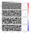 |
Fig. 2 Maps of bolometric intensity and vertical magnetic field representative of the three simulation phases. The time instants of the bolometric intensity during phases 1 (first column), 2 (second column), and 3 (third column) are normalized to their respective mean intensities. The fourth column displays the vertical magnetic field at z = 0 during phase 3 at the same time instant as for the third column. The rows (from top to bottom) correspond to the spectral types K8V, K2V, G2V, and F5V. The red arrows in the K2V model indicate non-magnetic bright points, whereas the red contours in the third column denote the MBFs detected by the algorithm (see Sect. 5.3 and Appendix B). |
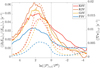 |
Fig. 3 Time-averaged profiles of 〈∂tEm〉z/〈Em〉z (solid lines, left axis, smoothed for clarity with a moving average of width 10∆z) and computed during the kinematic phase, and of 〈|∇v|〉z,t (dashed lines, right axis) for the four models K8V, K2V, G2V, and F5V. The black dotted line denotes the geometrical height z = 0. To the left of this line is the convection zone; the photosphere is to the right. |
5 Saturation phases
As discussed in Sect. 2.3, the bottom boundary condition CB = 0 prevents replenishment from outside the domain of the magnetic field pumped out of the domain across its bottom boundary. Consequently, the saturation level reached during phase 2 can be considered to be a lower limit for the magnetic energy reached in our models. As is discussed in the following, the amount of magnetic energy generated with this bottom boundary condition does not have a noticeable impact on the plasma flows and on the radiative field, consistently with the solar results in Rempel (2014). For this reason, we only briefly discuss the results of phase 2, while putting more emphasis on the results of phase 3, which displays MBFs similar to those observed on the Sun (see Sect. 5.3).
5.1 Characteristics of the magnetic field
From Fig. 1 it is clear that the simulations attain a magnetic energy that is significantly lower in phase 2 than in phase 3 for all spectral types. In addition, during both saturation phases, the magnetic-to-kinetic energy ratio, averaged over the convection zone, is independent of the stellar model, with 〈〈Em〉c/〈Ek〉c〉t = 1.3–2.5% during phase 2 and 〈〈Em〉c/〈Ek〉c〉t = 17–21% during phase 3.
A deeper insight into the properties of the magnetic fields generated by SSD action provides the first four rows of Table 4, which display the rms of Bz and B (rows 1 and 2, respectively) and the horizontal averages of |Bz| and B (rows 3 and 4, respectively) at τR = 1 and time averaged over phase 3, with B = |B|. Additionally, the left panel of Fig. 4 shows 〈B〉z,t as a function of ln(〈P〉z,t/P0) (solid lines). Interestingly, the magnetic field strengths are independent of the spectral type. These amplitudes are similar to the solar value found in Rempel (2014), which for model O16bM is 〈B〉τ=1,t = 160 G. Moreover, we obtain magnetic field strengths similar to those found in Bhatia et al. (2022), which are in the range 〈B〉τ=1,t = 103–188 G. The main difference with the results in Bhatia et al. (2022) are the magnetic field strengths for stars of spectral type F, which in our case are slightly lower than for the G2V model and not about 40% higher as in Bhatia et al. (2022). The stronger magnetic field for the F3V model with respect to the cooler models is linked to a larger fraction of kinetic energy converted into magnetic energy, which we do not observe for our F5V model (as discussed later in this section). This could be related to the different log ɡ and Teff values used for the F5V and F3V models. Moreover, comparing 〈Brms(τR = 1)〉t to the values reported in Beeck et al. (2015, their Table 2), we see that our results are similar to the results of the magnetic simulations that started with a uniform vertical seed field of Bz = 20 G.
To investigate the reason for the magnetic field strength and for the magnetic pressure, Pm = B2/(8π) (row 8 of Table 4), being approximately independent of the spectral type, the left panel of Fig. 4 also displays the amplitudes of the dynamic equipartition field, Eq. (6), as a function of height for the four models during the kinematic phase (dashed lines). We see that the equipartition fields are of similar strengths for all models at all heights. This means that higher densities, and hence higher gas pressures in cooler models are compensated for by higher velocities in hotter models (see rows 7 and 11 of Table 4), with the two effects approximately balancing each other.
In addition, at the optical surface, Beq dyn decreases by approximately 6% from phase 1 to phase 3 for all models (see row 5 of Table 4), which corresponds to a decrease in the kinetic energy density of approximately 11–12% (see rows 9 and 10 of Table 4, with Pdyn = ρv2/2). This is mainly related to a decrease in the rms velocity from phase 1 to phase 3 (row 11 of Table 4), and it means that the saturation mechanism of the SSD is similar for all spectral types and that it is independent of the growth rates discussed in Sect. 4. The magnetic to dynamic equipartition field ratios show very similar amplitudes for all models, with B/Beq dyn ≃ 0.2 near the surface and increasing up to 0.3 near the bottom boundary.
The right panel of Fig. 4 displays the ratio of the horizontal, Bh, to the absolute vertical magnetic field strength for the four models, time averaged over phase 3. For an isotropically distributed magnetic field, one would expect this ratio to be π/2. For the present simulations, the magnetic fields are slightly more vertical than horizontal in the convection zone, in agreement with the findings reported in Bhatia et al. (2022). On the other hand, magnetic fields are close to isotropy at the optical surface, and become more horizontal in the photosphere, in particular for the coolest models. A peak in the solar photosphere of the horizontal-to-vertical magnetic field ratio is consistent with the findings in Steiner et al. (2008), where it is shown that the predominance of horizontal fields in the photosphere can be considered a consequence of the flux expulsion process by overshooting convection. This is also consistent with the results in Sect. 4.6 of Rempel (2014). We note that the strong decrease in the Bh-to-|Bz| ratios near the top boundary is due to the boundary conditions, which impose a vertical magnetic field at the top of the domain.
Finally, Fig. 5 displays the flux-based probability density function (PDF), PDFΦ(|Bz|) = |Bz|PDF(|Bz|)/Φtot (solid lines, left axis), and the corresponding empirical distribution function,  (dashed lines, right axis), for the four models at z = 0 (left panel) and τR = 1 (right panel) during phase 3, where Φtot is the absolute magnetic flux trough the area LxLy and PDF(|Bz|) the probability density function of |Bz|. PDFΦ(|Bz|)dBz represents the probability that a given flux element, dΦ, has a flux density in the interval [|Bz|, |Bz + dBz|], whereas EDFΦ(|Bz|) gives the contribution to the total absolute magnetic flux from magnetic fields weaker than |Bz| (Steiner 2003). The peaks of PDFΦ(|Bz|) are located at approximately the same flux density, about |Bz| = 15–25 G, for all four models, and both at z = 0 and τR = 1. At z = 0, the four PDFΦ(|Bz|) display similar behaviour up to |Bz| = 300 G, while they extend to stronger magnetic fields for cooler models than for hotter models. On the other hand, at τR = 1, the profiles of PDFΦ(|Bz|) show similar behaviour also at high flux densities, although the peaks of the two coolest models at |Bz| ≃ 20 G are higher than for models G2V and F5V. Overall, these results are similar to the findings in Beeck et al. (2015) for the simulations that started with B0 = 20 G. We note that our simulations do not display a second peak of PDFΦ(|Bz|) at |Bz| ≃ 1000–2000 G, as observed for simulations that started with an initial magnetic field higher than or equal to 50 G (see e.g. Beeck et al. 2015; Salhab et al. 2018). Likewise, the EDFΦ(|Bz|) also shows similar profiles for all models, except for large |Bz| at z = 0. The EDFΦ(|Bz|) in Fig. 5 show that about half of the absolute magnetic flux has a field strength |Bz| < 200 G for all models and that kG fields contribute at z = 0 to Φtot by 9%, 6%, 7%, and 1% for models K8V, K2V, G2V, and F5V, respectively. Thus, more than 90% of the magnetic flux through the stellar surface has a field strength of less than 1 kG. More about strong magnetic flux concentrations can be found in Sect. 5.3.
At the origin of the transfer of energy from the kinetic to the magnetic energy reservoir is the work done by the Lorentz force on the plasma. Considering the second saturation phase and integrated over the entire convection zone of the model, this work is actually substantial compared to the radiative flux from the stellar surface. Indeed,  −0.57, −0.36, −0.35, and −0.34 for model K8V, K2V, G2V, and F5V, respectively, where j = ∇ × B/(4π) and Frad is the radiative flux from the stellar surface. Thus, the energy flux transferred by the Lorentz force of the SSD is of the order of the stellar luminosity, although the exact number strongly depends of the numerical set-up.
Properties of the atmospheres of the four models during the kinematic and the second saturation phases.
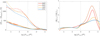 |
Fig. 4 Magnetic field structure for the four models. Left: temporal and horizontal averages of the magnetic (solid lines) and dynamic equipartition (dashed lines) fields. Right: horizontal to vertical magnetic field ratio. Temporal averages of the dynamic equipartition and of the magnetic field strengths are evaluated during phases 1 and 3, respectively. The black dotted lines denote the geometrical height z = 0; to the left of the line is the convection zone, and to the right the photosphere. |
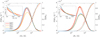 |
Fig. 5 Magnetic flux distributions. Flux-based probability density functions (solid lines, left axis) and corresponding empirical distribution functions (dashed lines, right axis) as a function of |Bz| at z = 0 (left panel) and τR = 1 (right panel) for the four models during phase 3. The insets in the top left corners of the larger panels display zoomed-in images of PDFΦ at high magnetic field strengths. |
5.2 Impact of SSD action
Row 12 of Table 4 displays the visible continuum rms intensity contrast of the granular pattern, defined as
 (13)
(13)
with 〈Ibol〉h denoting the average of the bolometric intensity over the horizontal plane. Consistently with the discussion of Fig. 2 in Sect. 3.2, crms increases from the coolest to warmer models. Row 12 of Table 4 also shows that crms decreases from phase 1 to phase 3 for all models, and that this decrease is greater with increasing Teff. To investigate this behaviour, we display in Fig. 6 the PDF of the relative intensity fluctuations,  , for the four models during phases 1 (solid lines) and 3 (dashed lines). The appearance of bright features in the intergranular lanes in phase 3 (see red contours in the third column of Fig. 2) manifests in Fig. 6 as a decrease in the PDFs at the low end, except for the K8V model, and the emergence of an extra tail at the high end of the intensity distributions (solid vs. dashed lines). However, the decrease in crms from phases 1 to 3 is not related to changes in the tails of the PDFs, which have much lower realization rates than the core of the distribution, but rather to changes near the centre of the PDFs (see inset in the top right corner of Fig. 6).
The lack of MBFs in Fig. 2 during phase 2 (cf. second and third columns) is due to the low saturation level reached by the magnetic energy with CB = 0. Indeed, 〈B〉τ=1,t ≃ 29–53 G during phase 2, which is about a factor of three smaller than when using CB ≠ 0 (cf. row 4 of Table 4). As also shown by Rempel (2014) for the solar case, this is not enough magnetic flux to form kG flux concentrations. We note that tiny bright dots within the intergranular lanes occur in all spectral types during phases 1 and 2, and are particularly conspicuous in the K2V model. Two of them are indicated by red arrows in Fig. 2. These dots are not of magnetic origin, but they form from swirling downdrafts due to the low pressure at the centre of the vortices, giving rise to non-magnetic bright points (Vögler et al. 2005; Calvo et al. 2016).
The impact of the magnetic fields generated by SSD action on the granulation is demonstrated in Fig. 7, which displays the integral length scale of vertical velocity fluctuations, Eq. (5), averaged over phases 1 and 3 (solid and dashed lines, respectively). The convection zone (left of the black dotted line) shows a 5%–10% reduction in Lint from phase 1 to 3 for all models. As explained in Bhatia et al. (2022), a reduction in kinetic energy because of SSD action, and a corresponding reduction in con-vective velocities (rows 9–11 of Table 4), leads to a reduction in the pressure scale height. This, in turn, explains the decrease in Lint from phase 1 to 3. On the other hand, differences at the optical surface are much smaller. Above the optical surface (to the right of the black dotted line), models K8V, K2V, and G2V also display a reduction in Lint, whereas the hottest model, F5V, shows an opposite trend.
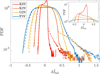 |
Fig. 6 Probability density functions of the relative intensity fluctuations |

5.3 Characteristics of magnetic bright features
5.3.1 Properties of magnetic flux concentrations
During phase 3, all the stellar models show bright features located in the intergranualar space, where strong magnetic fields form magnetic flux concentrations (see the red contours in the third column of Fig. 2). These correspond to the MBFs, also known as magnetic filigree, magnetic bright points, or G-band bright points, observed with high-resolution instruments on the solar disk (Dunn & Zirker 1973; Mehltretter 1974; Berger & Title 1996). We now characterize the MBFs observed in our models during phase 3.
As the name suggests, MBFs harbour strong magnetic fields and are brighter than their surrounding space. Therefore, to identify MBFs in the simulations and perform a statistical analysis, we developed an algorithm based on the following conditions: pixels corresponding to an individual MBF have Ibol and |Bz|(z = 0) larger than some given thresholds and they are located within a closed contour of sufficiently large area. For the intensity threshold we choose Ibol > 〈Ibol〉h,t; for the absolute vertical magnetic field we use |Bz|(z = 0) > 875.7, 704.2, 700.3, and 584.2 G for model K8V, K2V, G2V, and F5V, respectively, and we discard contours enclosing fewer than 20 pixels, with one pixel corresponding to an area of ∆x∆y. A discussion of these criteria and more details on the algorithm are given in Appendix B.
The first row of Table 5 gives the number of MBFs per snapshot found with the algorithm. We see that the K2V and G2V models display the highest number of MBFs, while the K8V model counts less than half their MBFs. Additionally, Fig. 8 displays the PDFs of the area of MBFs. The distributions are very similar for the four models and approximately follow an exponential function, with more MBFs of small areas and fewer MBFs of large areas. Since the four models have similar MBF area PDFs, but different numbers of MBFs per snapshot, the fraction of total area covered by MBFs changes among the four models, with the K2V and G2V models having the largest fraction (see second row of Table 5). This is also in qualitative agreement with the third column of Fig. 2, which displays more pixels covered by MBFs for the K2V and G2V models than for the other two models.
Rows 3–10 of Table 5 give the magnetic properties of the MBFs, where 〈q〉MBF denotes first computing the quantity q = Bz,rms, max(|Bz|), and Bh|BZ| over the area of each MBF individually, and then averaging over the sample of all the identified MBFs. We note that averaging over each MBF individually weights the smaller MBFs more than the larger ones (see Fig. 8). Nevertheless, this does not affect the trends discussed in the following1. Rows 3 and 5 of Table 5 show that the rms and the maximum of the absolute vertical magnetic field decreases as Teff increases at z = 0. Here, max(|Bz|) is evaluated as the average of |Bz| over the nine pixels closest to the maximum value of |Bz| of each MBF. At τR = 1 the differences in the rms and maximum values of |Bz| for the four models are smaller than at z = 0, but the decreasing trend with increasing Teff is still significant (rows 4 and 6 of Table 5). This is different from what is found for magnetic simulations that started from a homogeneous vertical field of 50 G in Steiner et al. (2014) and Salhab et al. (2018), where the field strength at τR = 1 is independent of the spectral type.
Rows 7 and 8 of Table 5 show the fraction of vertical magnetic flux and magnetic energy contained by the MBFs with respect to the full horizontal plane at z = 0. Even if their area is less than 1% of the horizontal domain, MBFs contain a significant fraction of the magnetic flux and magnetic energy. Moreover, as is the case for the number density of MBFs, their contribution to the magnetic flux and magnetic energy is also larger for the K2V and G2V models than for K8V and F5V.
For solar simulations carried out with the MURaM code under similar conditions, it is found that kG flux concentrations contribute about 9–16% to the total magnetic energy, depending on the resolution (Rempel 2014). This is consistent with the present results.
Rows 9 and 10 of Table 5 display the ratio of Bh to |Bz| in the MBFs at z = 0 and τR = 1, respectively. At z = 0, |Bz| is much larger than Bh, indicating that the magnetic field is preferentially vertical in the MBFs. This is not true at τR = 1, in particular for the MBFs of the K2V and G2V models, for which the magnetic field is instead isotropically distributed.
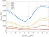 |
Fig. 7 Integral length scale of vertical velocity fluctuations for the four models. The solid and dashed coloured lines denote phases 1 and 3, respectively. The black dotted line denotes the geometrical height z = 0; to the left of the line is the convection zone, and to the right the photosphere. |
Characteristics of the magnetic bright features identified by the algorithm of Appendix B for the four models.
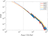 |
Fig. 8 Probability density functions of MBF areas for the four models. The black dotted line denotes the 20-pixel threshold, below which MBFs are discarded. The dashed lines are the extension of the PDF as if small MBFs were retained. |
5.3.2 Discussion
We now investigate the reason for the decreasing field strength of MBFs with increasing effective temperature, showing that it is the result of two competing effects: the increasing near-surface opacities and increasing evacuation efficiency with increasing Teff. As discussed, for example, in Salhab et al. (2018), in the present range of temperatures and gas pressures an increase in effective temperature leads to an increase in opacity, which in turn gives higher gas pressures at the optical surface for cooler in comparison to hotter models (row 7 of Table 4). Consequently, the thermal equipartition field strength,  , decreases with increasing Teff (row 6 of Table 4), thus leading to flux concentrations of lower magnetic field strength at higher effective temperatures. However, as the decreasing trend of Beq,th with increasing Teff is much more pronounced than for the magnetic field strength (cf. row 6 of Table 4 with rows 3 and 5 of Table 5), the opacity effect alone is not able to explain the results in Table 5.
To further investigate the trend displayed by the magnetic field strength of MBFs with increasing Teff, we compute the mass-density, temperature, and pressure contrasts of the MBFs at z = 0 and τR = 1 as cq(z = 0) = (〈q〉MBF − 〈q〉z=0)/〈q〉z=0 and cq(τR = 1) = (〈q〉MBF − 〈q〉τ=1)/〈q〉τ=1, respectively, with q = ρ, T, or Pgas. These are displayed in rows 11–16 of Table 5. The mass density contrast at z = 0 is significantly lower than zero for all models, and it strongly decreases with increasing Teff. This indicates that the degree of evacuation of MBFs strongly increases with increasing Teff. As discussed in Salhab et al. (2018), in the convective collapse framework (Parker 1978; Webb & Roberts 1978; Spruit 1979), a more efficient evacuation is associated with a more efficient MBF formation process, hence leading to a higher ratio of the magnetic to thermal equipartition field strengths (cf. rows 5 and 6 of Table 5 with row 6 of Table 4). The higher efficiency of MBF formation at high Teff is due to the larger superadiabaticity of hot models with respect to the cooler ones (see e.g. Salhab et al. 2018; Beeck et al. 2013; Magic et al. 2013). At τR = 1 the MBF evacuation is much lower than at z = 0 (cf. rows 11 and 12 of Table 5). This is due to the fact that the strong magnetic field in MBFs, in combination with horizontal pressure balance, leads to a downward shift of the optical surface with respect to the surrounding atmosphere. Therefore, the τR = 1 surface is highly corrugated and it is deeply depressed within MBFs, thus reaching higher density values. The compensating effect of the evacuation process explains the milder dependence of the magnetic field strength of MBFs on Teff, in contrast to the strong dependence of Beq,th on Teff. The two competing effects are probably also at the origin of the increasing trend for AMBF/Atot, ΦMBF/Φtot, and Em,MBF/Em,tot for models K8V, K2V, and G2V, followed by a decrease in these three quantities when further increasing Teff from 5766 K to 6506 K (see rows 2, 7, and 8 of Table 5).
The strong magnetic field in MBFs mitigates the horizontal heat exchange responsible for thermal equilibrium, resulting in colder temperatures at 𝓏 = 0 in MBFs with respect to the surrounding plasma at the same geometrical height (see row 13 of Table 5). On the other hand, as the visible surface within MBFs is located below the 𝓏 = 0 level, the MBF temperature at τR = 1 is higher than the normal surface temperature (see row 14 of Table 5), although it is lower than the averaged temperature at the geometrical height level of the depressed surface. As temperature deviations are much smaller than mass density deviations in MBFs (cf. rows 13–14 with rows 11–12 of Table 5), cP ≈ cρ both at 𝓏 = 0 and τR = 1 (cf. rows 15–16 with rows 11–12 of Table 5).
Finally, we report the average shift of the τR = 1 surface in MBFs with respect to the 〈τR〉𝓏 = 1 surface in row 17 of Table 5, denoted WD in reminiscence of the Wilson depression of sunspots. It results that WD strongly increases with increasing Teff. Although the increase in the pressure scale height with increasing Teff (see Table 1) could explain this trend, WD increases more rapidly than HP, consistently with results in Steiner et al. (2014) and Salhab et al. (2018). This, again, is due to the increased evacuation efficiency of hotter spectral models with respect to the cooler ones.
6 Conclusions
In the present paper we numerically investigated the action of a small-scale dynamo operating in the near-surface layers of four cool main-sequence stars of spectral types K8V, K2V, G2V, and F5V. The numerical domains were set up to ensure similar Reynolds and magnetic Reynolds numbers for all models. Starting from a seed field of 1 mG, all simulations display the operation of a SSD close beneath the stellar surface, which transfers energy from the kinetic to the magnetic reservoir, mostly through stretching of magnetic fields by velocity shear. As the four models have different turnover times, the SSD growth rates are different for the four stellar models; the highest and lowest growth rates are for the K2V and F5V models, respectively. When normalizing the time in the system by the turnover time, the growth rates are very similar, in agreement with the fact that the magnetic Reynolds and Prandtl numbers are similar for the four models.
When a balance between amplification of the magnetic field and losses of magnetic energy is attained, the simulations reach a statistical steady-state. The SSD field strength reached in the saturation phase is similar in all models, irrespective of the kinematic SSD growth rate. However, the bottom boundary condition strongly affects the amount of magnetic energy that can be sustained during the saturation phase. In particular, the magnetic field amplified by the SSD has a noticeable impact on plasma flows only if a partial replenishment of the magnetic energy that is pumped out across the bottom boundary is allowed to enter from outside the computational domain. In this case, 1721% of the energy is transferred from the kinetic energy to the magnetic energy reservoir. This leads to a reduction in the convective velocities that is enough to reduce the convective horizontal length scale in the convection zone by 5%–10%, although not at the visible surface. In this situation, the SSD magnetic fields display properties very similar to the simulations that started with a uniform initial field of B𝓏 = 20 G. The rms of the absolute magnetic field strength at the visible surface is approximately 200 G, independent of the spectral type. Moreover, while the magnetic field is close to isotropic near the τR = 1 level, it is predominantly horizontal further up in the photosphere for all models.
In the saturation stage including replenishment of pumped out magnetic fields, the SSD action also results in the formation of strong kG magnetic flux concentrations at the surface, which appear as MBFs on the intensity map of all stellar models. Strong magnetic flux concentrations are twice as numerous in the K2V and G2V models as in the K8V and F5V models. It results in an absolute vertical magnetic flux located in the MBFs, normalized to the total absolute vertical magnetic flux, that is about twice in the K2V and G2V models with respect to the K8V and F5V models. However, more than 90% of the magnetic flux through any of these stellar surfaces has a field strength less than 1 kG. The vertical component of the field strength of the MBFs at optical depth unity increases from approximately 1.0 to 1.6 kG with decreasing temperature from F5V to K8V due to the competing effects of opacity and formation efficiency.
Overall, these results give a deeper insight into the operation of the SSD in the near-surface layers of cool main-sequence stars and the self-organization of magnetic fields into kG flux concentrations. In addition, the present simulations provide the basis for investigating the impact of the SSD self-generated MBFs on interferometric and planet transit observations, thus extending the work in Chiavassa et al. (2010) and Chiavassa et al. (2017) to magnetic phenomena. In the future, it will be important to broaden the parameter space of the numerical models by including more stars, where the SSD magnetic fields could have stronger effects, such as stars hotter than those in the F5V model (see e.g. Bhatia et al. 2022). An ideal case could be Atype stars with shallow convection zones. This would mitigate the impact of the bottom boundary condition on the simulation results as the convection zones can be fully contained in the numerical domain.
Acknowledgements
This work was supported by the Swiss National Science Foundation under grant ID 200020_182094. Part of the numerical simulations were carried out on Piz Daint at CSCS under project IDs s1059, s1172, and u14, and the rest was carried out on the HPC ICS cluster at USI. We sincerely thank the anonymous referee for the careful reading of the manuscript and his/her comments, which helped us to improve the quality of the paper.
Appendix A Results in normalized units
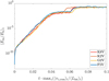 |
Fig. A.1 Temporal profiles of magnetic-to-kinetic energy ratios averaged over the convection zone, with the time coordinate normalized to the turnover times of the four models. |
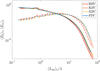 |
Fig. A.2 Kinetic and magnetic energy spectra (solid and dashed lines, respectively) time averaged over the kinematic phase and normalized to their surface area for the four models K8V, K2V, G2V, and F5V. The x-axis is the wave number normalized to the integral length scale. It is also visible that the magnetic energy resides mostly at small scales, as expected for a SSD. |
When comparing the physical properties of the four simulations, it can be useful to normalize the time and length scales in the models to the characteristic scales in the system, which are the turnover time and the integral length scale, respectively. Since the efficiency of the SSD is greatest close to ln(〈P〉𝓏,t/P0) = 2 (see Sect. 4), the integral length scales discussed in the following of this Appendix are computed at this position (see also Fig. 7), whereas the turnover times τ are given in Table 1.
In Fig. A.l we display the temporal profiles of the magnetic-to-kinetic energy ratio averaged over the convection zone, with the time of each model normalized to the corresponding turnover time. During the kinematic phase, the four curves are very close to each other. This is an expression of the small deviations of the normalized SSD growth times among the four models (see the last column of Table 2). It is also in agreement with the mild variations in the flow parameters of the four models (see second, third, and fourth columns of Table 2).
Figure A.2 displays the kinetic (solid lines) and magnetic (dashed lines) energy spectra time averaged over the kinematic phase. At each time instant, each spectrum is normalized to its integral area before performing the time average. The length scales are normalized to the integral length scale of each model. It results that, in normalized units, the spectra of the four models are very close to each other. This is again an expression of the small variations in the flow parameters among the four models (see second, third, and fourth columns of Table 2).
Appendix B Magnetic bright feature recognition
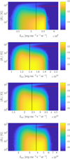 |
Fig. B.1 Bivariate distribution, in logarithmic scale, of Ibol and |B𝓏 | during phase 3. The rows (from top to bottom) correspond to the spectral types K8V, K2V, G2V, and F5 V, respectively. The black vertical and red horizontal lines denote 〈Ibol〉h,t and B𝓏,tbreshoid, respectively. |
Magnetic flux concentrations that form during phase 3 lead to the emergence of bright features in the intergranular space. Thus, it is natural to set a condition on |B𝓏| and on Ibol in order to identify magnetic bright features (MBFs). More precisely, combining the two-dimensional maps of |B𝓏|(𝓏 = 0) with those of Ibol, we define an individual MBF as the area with |B𝓏| and Ibol above a given threshold and within a closed contour.
The |B𝓏|(z = 0) and Ibol thresholds are defined as follows. Figure B.1 displays the logarithm of the bivariate distribution of Ibol and |B𝓏|(𝓏 = 0) during phase 3 for the four models. An extended tail of bright magnetic pixels can be clearly seen in the top right part of each panel. These are the MBFs. Thus, for the Ibol threshold, we simply use the averaged bolometric intensity, 〈Ibol〉h,t, indicated by the black vertical lines in Fig. B.1. Furthermore, we set the |B𝓏| threshold, B𝓏,threshold, as the local minimum of the distribution of |B𝓏|(Ibol > 〈Ibol〉h,t), indicated by the red horizontal lines in Fig. B.1. This gives B𝓏,threshold = 875.7, 704.2, 700.3, and 584.2 G for models K8V, K2V, G2V, and F5V, respectively.
This approach for the MBF identification is different from that used by Salhab et al. (2018), where one threshold on the magnetic field alone is used, and with the same B𝓏,threshold for all models. This for two reasons. First, the PDFΦ(|B𝓏|) values in Fig. 5 do not display a secondary peak at high magnetic flux densities as in Beeck et al. (2015) or Salhab et al. (2018). On the other hand, when considering |B𝓏|(Ibol > 〈Ibol〉h,t) alone, one can clearly discern a strong field component in Fig. B.1. This justifies the use of a threshold on Ibol for identifying an MBF. Second, the strong field component at τR = 1 of the present SSD simulations shows a stronger dependence on Teff than for simulations that started with an initial magnetic field higher than or equal to 50 G (see e.g. Beeck et al. 2015; Salhab et al. 2018). This justifies the use of a B𝓏,threshold that depends on Teff.
As an additional constraint, we also require MBFs to occupy an area equal to or larger than 20 pixels, with the area of a pixel being ∆x∆y. We do this to discard small transient features. Tests with a reasonable range of thresholds (between 0 and 30 pixels) proved that the precise choice of the threshold does not impact the trends discussed in Sect. 5.3.
References
- Batchelor, G. K. & Taylor, G. I. 1950, Proc. Roy. Soc. Lond. Ser. A Math. Phys. Sci., 201, 405 [NASA ADS] [Google Scholar]
- Beeck, B., Schüssler, M., & Reiners, A. 2011, 16th Cambridge Workshop on Cool Stars, Stellar Systems, and the Sun, eds. C. M. Johns-Krull, M. K. Browning, & A. A. West (San Francisco: Astronomical Society of the Pacific), ASP Conf. Ser., 448, 1071 [NASA ADS] [Google Scholar]
- Beeck, B., Cameron, R. H., Reiners, A., & Schüssler, M. 2013, A&A, 558, A48 [NASA ADS] [CrossRef] [EDP Sciences] [Google Scholar]
- Beeck, B., Schüssler, M., Cameron, R. H., & Reiners, A. 2015, A&A, 581, A42 [NASA ADS] [CrossRef] [EDP Sciences] [Google Scholar]
- Berdyugina, S. V. 2005, Living Rev. Solar Phys., 2, 1 [NASA ADS] [CrossRef] [Google Scholar]
- Berger, T. E., & Title, A. M. 1996, ApJ, 463, 365 [NASA ADS] [CrossRef] [Google Scholar]
- Bhatia, T. S., Cameron, R. H., Solanki, S. K., et al. 2022, A&A, 663, A166 [NASA ADS] [CrossRef] [EDP Sciences] [Google Scholar]
- Brandenburg, A., & Subramanian, K. 2005, Phys. Rep., 417, 1 [NASA ADS] [CrossRef] [Google Scholar]
- Calvo, F., Steiner, O., & Freytag, B. 2016, A&A, 596, A43 [NASA ADS] [CrossRef] [EDP Sciences] [Google Scholar]
- Cattaneo, F. 1999, ApJ, 515, L39 [Google Scholar]
- Chiavassa, A., Haubois, X., Young, J. S., et al. 2010, A&A, 515, A12 [CrossRef] [EDP Sciences] [Google Scholar]
- Chiavassa, A., Caldas, A., Selsis, F., et al. 2017, A&A, 597, A94 [NASA ADS] [CrossRef] [EDP Sciences] [Google Scholar]
- Donati, J.-F., & Landstreet, J. 2009, ARA&A, 47, 333 [NASA ADS] [CrossRef] [Google Scholar]
- Dunn, R. B., & Zirker, J. B. 1973, Solar Phys., 33, 281 [NASA ADS] [CrossRef] [Google Scholar]
- Evans, C. R., & Hawley, J. F. 1988, ApJ, 332, 659 [Google Scholar]
- Fan, Y. 2021, Living Rev. Solar Phys., 18, 5 [CrossRef] [Google Scholar]
- Freytag, B. 2013, Mem. Soc. Astron. Ital. Suppl., 24, 26 [Google Scholar]
- Freytag, B. 2017, Mem. Soc. Astron. Ital., 88, 12 [Google Scholar]
- Freytag, B., Steffen, M., Ludwig, H.-G., et al. 2012, J. Comput. Phys., 231, 919 [Google Scholar]
- Gustafsson, B., Edvardsson, B., Eriksson, K., et al. 2008, A&A, 486, 951 [NASA ADS] [CrossRef] [EDP Sciences] [Google Scholar]
- Harten, A., Lax, P. D., & van Leer, B. 1983, SIAM Rev., 25, 35 [Google Scholar]
- Heiter, U., Jofré, P., Gustafsson, B., et al. 2015, A&A, 582, A49 [NASA ADS] [CrossRef] [EDP Sciences] [Google Scholar]
- Käpylä, P. J., Käpylä, M. J., & Brandenburg, A. 2018, Astron. Nachr., 339, 127 [CrossRef] [Google Scholar]
- Khomenko, E., Vitas, N., Collados, M., & de Vicente, A. 2017, A&A, 604, A66 [NASA ADS] [CrossRef] [EDP Sciences] [Google Scholar]
- Kitiashvili, I. N., Kosovichev, A. G., Mansour, N. N., & Wray, A. A. 2015, ApJ, 809, 84 [NASA ADS] [CrossRef] [Google Scholar]
- Kochukhov, O., Petit, P., Strassmeier, K. G., et al. 2017, Astron. Nachr., 338, 428 [Google Scholar]
- Ludwig, H. G. 1992, PhD thesis, University of Kiel, Germany [Google Scholar]
- Magic, Z., Collet, R., Asplund, M., et al. 2013, A&A, 557, A26 [NASA ADS] [CrossRef] [EDP Sciences] [Google Scholar]
- Martins Afonso, M., Mitra, D., & Vincenzi, D. 2019, Proc. Roy. Soc. A: Math. Phys. Eng. Sci., 475, 20180591 [Google Scholar]
- Mehltretter, J. P. 1974, Solar Phys., 38, 43 [NASA ADS] [CrossRef] [Google Scholar]
- Nguyen, C. T., Costa, G., Girardi, L., et al. 2022, A&A, 665, A126 [NASA ADS] [CrossRef] [EDP Sciences] [Google Scholar]
- Nordlund, A. 1982, A&A, 107, 1 [Google Scholar]
- Parker, E. N. 1978, ApJ, 221, 368 [NASA ADS] [CrossRef] [Google Scholar]
- Pietarila Graham, J., Cameron, R., & Schüssler, M. 2010, ApJ, 714, 1606 [Google Scholar]
- Rackham, B. V., Espinoza, N., Berdyugina, S. V., et al. 2023, RAS Tech. Instrum., 2, 148 [NASA ADS] [CrossRef] [Google Scholar]
- Ramelli, R., Bianda, M., Berdyugina, S., Belluzzi, L., & Kleint, L. 2019, ASP Conf. Ser., 526, 283 [NASA ADS] [Google Scholar]
- Reiners, A. 2012, Living Rev. Solar Phys., 9, 1 [NASA ADS] [CrossRef] [Google Scholar]
- Rempel, M. 2014, ApJ, 789, 132 [Google Scholar]
- Riva, F., & Steiner, O. 2022, A&A, 660, A115 [NASA ADS] [CrossRef] [EDP Sciences] [Google Scholar]
- Roe, P. L. 1986, Annu. Rev. Fluid Mech., 18, 337 [NASA ADS] [CrossRef] [Google Scholar]
- Salhab, R. G., Steiner, O., Berdyugina, S. V., et al. 2018, A&A, 614, A78 [NASA ADS] [CrossRef] [EDP Sciences] [Google Scholar]
- Seta, A., & Federrath, C. 2021, Phys. Rev. Fluids, 6, 103701 [NASA ADS] [CrossRef] [Google Scholar]
- Solanki, S. K., Inhester, B., & Schüssler, M. 2006, Rep. Progr. Phys., 69, 563 [CrossRef] [Google Scholar]
- Spruit, H. C. 1979, Solar Phys., 61, 363 [CrossRef] [Google Scholar]
- Steiner, O. 2003, A&A, 406, 1083 [NASA ADS] [CrossRef] [EDP Sciences] [Google Scholar]
- Steiner, O., Rezaei, R., Schaffenberger, W., & Wedemeyer-Böhm, S. 2008, ApJ, 680, L85 [NASA ADS] [CrossRef] [Google Scholar]
- Steiner, O., Salhab, R., Freytag, B., et al. 2014, PASJ, 66, S5 [NASA ADS] [Google Scholar]
- Strassmeier, K. G. 2009, A&ARv, 17, 251 [Google Scholar]
- Thaler, I., & Spruit, H. C. 2015, A&A, 578, A54 [NASA ADS] [CrossRef] [EDP Sciences] [Google Scholar]
- Vögler, A. & Schüssler, M. 2007, A&A, 465, L43 [NASA ADS] [CrossRef] [EDP Sciences] [Google Scholar]
- Vögler, A., Shelyag, S., Schüssler, M., et al. 2005, A&A, 429, 335 [Google Scholar]
- Webb, A. R., & Roberts, B. 1978, Solar Phys., 59, 249 [NASA ADS] [CrossRef] [Google Scholar]
- Wedemeyer-Böhm, S., Lagg, A., & Nordlund, Å. 2009, Space Sci. Rev., 144, 317 [Google Scholar]
- Witzke, V., Duehnen, H. B., Shapiro, A. I., et al. 2023, A&A, 669, A157 [NASA ADS] [CrossRef] [EDP Sciences] [Google Scholar]
Repeating the analysis with averages weighted by the MBF area confirms the trends in Table 5. They are just more pronounced.
All Tables
Basic physical and numerical parameters for the four simulation models and close Gaia benchmark stars.
Initial and final physical times for each phase and each stellar model and number of time instances of full data output of the entire physical domain used for post-processing.
Properties of the atmospheres of the four models during the kinematic and the second saturation phases.
Characteristics of the magnetic bright features identified by the algorithm of Appendix B for the four models.
All Figures
|
Fig. 1 Temporal profiles of magnetic to kinetic energy ratios averaged over the convection zone of the four models K8V, K2V, G2V, and F5V. The round, square, and diamond markers denote phase 1, phase 2, and phase 3, respectively. |
| In the text | |
|
Fig. 2 Maps of bolometric intensity and vertical magnetic field representative of the three simulation phases. The time instants of the bolometric intensity during phases 1 (first column), 2 (second column), and 3 (third column) are normalized to their respective mean intensities. The fourth column displays the vertical magnetic field at z = 0 during phase 3 at the same time instant as for the third column. The rows (from top to bottom) correspond to the spectral types K8V, K2V, G2V, and F5V. The red arrows in the K2V model indicate non-magnetic bright points, whereas the red contours in the third column denote the MBFs detected by the algorithm (see Sect. 5.3 and Appendix B). |
| In the text | |
|
Fig. 3 Time-averaged profiles of 〈∂tEm〉z/〈Em〉z (solid lines, left axis, smoothed for clarity with a moving average of width 10∆z) and computed during the kinematic phase, and of 〈|∇v|〉z,t (dashed lines, right axis) for the four models K8V, K2V, G2V, and F5V. The black dotted line denotes the geometrical height z = 0. To the left of this line is the convection zone; the photosphere is to the right. |
| In the text | |
|
Fig. 4 Magnetic field structure for the four models. Left: temporal and horizontal averages of the magnetic (solid lines) and dynamic equipartition (dashed lines) fields. Right: horizontal to vertical magnetic field ratio. Temporal averages of the dynamic equipartition and of the magnetic field strengths are evaluated during phases 1 and 3, respectively. The black dotted lines denote the geometrical height z = 0; to the left of the line is the convection zone, and to the right the photosphere. |
| In the text | |
|
Fig. 5 Magnetic flux distributions. Flux-based probability density functions (solid lines, left axis) and corresponding empirical distribution functions (dashed lines, right axis) as a function of |Bz| at z = 0 (left panel) and τR = 1 (right panel) for the four models during phase 3. The insets in the top left corners of the larger panels display zoomed-in images of PDFΦ at high magnetic field strengths. |
| In the text | |
|
Fig. 6 Probability density functions of the relative intensity fluctuations |
| In the text | |
|
Fig. 7 Integral length scale of vertical velocity fluctuations for the four models. The solid and dashed coloured lines denote phases 1 and 3, respectively. The black dotted line denotes the geometrical height z = 0; to the left of the line is the convection zone, and to the right the photosphere. |
| In the text | |
|
Fig. 8 Probability density functions of MBF areas for the four models. The black dotted line denotes the 20-pixel threshold, below which MBFs are discarded. The dashed lines are the extension of the PDF as if small MBFs were retained. |
| In the text | |
|
Fig. A.1 Temporal profiles of magnetic-to-kinetic energy ratios averaged over the convection zone, with the time coordinate normalized to the turnover times of the four models. |
| In the text | |
|
Fig. A.2 Kinetic and magnetic energy spectra (solid and dashed lines, respectively) time averaged over the kinematic phase and normalized to their surface area for the four models K8V, K2V, G2V, and F5V. The x-axis is the wave number normalized to the integral length scale. It is also visible that the magnetic energy resides mostly at small scales, as expected for a SSD. |
| In the text | |
|
Fig. B.1 Bivariate distribution, in logarithmic scale, of Ibol and |B𝓏 | during phase 3. The rows (from top to bottom) correspond to the spectral types K8V, K2V, G2V, and F5 V, respectively. The black vertical and red horizontal lines denote 〈Ibol〉h,t and B𝓏,tbreshoid, respectively. |
| In the text | |
Current usage metrics show cumulative count of Article Views (full-text article views including HTML views, PDF and ePub downloads, according to the available data) and Abstracts Views on Vision4Press platform.
Data correspond to usage on the plateform after 2015. The current usage metrics is available 48-96 hours after online publication and is updated daily on week days.
Initial download of the metrics may take a while.