| Issue |
A&A
Volume 681, January 2024
|
|
|---|---|---|
| Article Number | A32 | |
| Number of page(s) | 11 | |
| Section | Stellar atmospheres | |
| DOI | https://doi.org/10.1051/0004-6361/202346460 | |
| Published online | 05 January 2024 | |
Small-scale dynamo in cool stars
III. Changes in the photospheres of F3V to M0V stars★
Max-Planck-Institut für Sonnensystemforschung,
Justus-von-Liebig Weg 3,
37077
Göttingen,
Germany
e-mail: bhatia@mps.mpg.de
Received:
20
March
2023
Accepted:
3
November
2023
Context. Some of the quiet solar magnetic flux could be attributed to a small-scale dynamo (SSD) operating in the convection zone. An SSD operating in cool main-sequence stars is expected to affect the atmospheric structure, in particular, the convection, and should have observational signatures.
Aims. We investigate the distribution of SSD magnetic fields and their effect on bolometric intensity characteristics, vertical velocity, and spatial distribution of the kinetic energy (KE) and magnetic energy (ME) in the lower photosphere of different spectral types.
Methods. We analyzed the SSD and purely hydrodynamic simulations of the near surface layers of F3V, G2V, K0V, and M0V stars. We compared the time-averaged distributions and power spectra in SSD setups relative to the hydrodynamic setup. The properties of the individual magnetic fields are also considered.
Results. The probability density functions with a field strength at the τ = 1 surface are quite similar for all cases. The M0V star displays the strongest fields, but relative to the gas pressure, the fields on the F3V star reach the highest values. In all stars, the horizontal field is stronger than the vertical field in the middle photosphere, and this excess becomes increasingly prominent toward later spectral types. These fields result in a decrease in the upflow velocities and a slight decrease in granule size, and also lead to formation of bright points in intergranular lanes. The spatial distribution of the KE and ME is also similar for all cases, implying that important scales are proportional to the pressure scale height.
Conclusions. The SSD fields have rather similar effects on the photospheres of cool main-sequence stars: a significant reduction in convective velocities, as well as a slight reduction in granule size and a concentration of the field to kilogauss levels in intergranular lanes that is associated with the formation of bright points. The distribution of the field strengths and energies is also rather similar.
Key words: convection / dynamo / stars: atmospheres / stars: late-type / stars: magnetic fields
Movies associated with Figs. 8 and 9 are available at https://www.aanda.org
© The Authors 2024
 Open Access article, published by EDP Sciences, under the terms of the Creative Commons Attribution License (https://creativecommons.org/licenses/by/4.0), which permits unrestricted use, distribution, and reproduction in any medium, provided the original work is properly cited.
This article is published in open access under the Subscribe to Open model.
Open Access funding provided by Max Planck Society.
1 Introduction
Magnetism in cool stars is ubiquitous. In addition, a significant number of cool stars show a solar-like activity cycle (Wilson 1978). The magnetic fields associated with these cycles are expected to arise from a large-scale dynamo operating in the interiors of cool stars (Brandenburg & Subramanian 2005; Charbonneau 2014). However, there is also an additional, cycle-independent component of stellar fields, the quiet-star magnetism. Based on detailed observations of the quiet Sun, (see, e.g., reviews by Solanki 1993; de Wijn et al. 2009; Sánchez Almeida & Martinez González 2011; Bellot Rubio & Orozco Suárez 2019) as well as based on the most recent simulations (Vögler & Schüssler 2007; Rempel 2014), this component was realized to be substantial and it was in part explained by invoking a small-scale dynamo (SSD) mechanism that amplifies magnetic fields via turbulent motions of the plasma. Recent global SSD simulations (Hotta & Kusano 2021; Hotta et al. 2022) showed that the generated field can be significantly superequipartition at small scales in the deep convection zone, and it is strong enough to affect the meridional circulation and the differential rotation profile. For stars other than the Sun, the influence of SSD fields on quiet-star phenomena such as granulation, pressure oscillations, and basal chromospheric activity remains to be studied.
Quiet-star magnetic fields also have the potential to affect our interpretation of radial velocity (RV) observations of stellar spectra. RV measurements allow the detection of exoplanets by accounting for Doppler shifts in stellar spectral lines due to a gravitation-induced wobble caused by the orbital motion of a planet. However, RVs can be affected by stellar magnetism. Starspots can affect RVs in multiple ways, for instance, via the Evershed effect (Solanki 2003; Rimmele & Marino 2006), while faculae reduce the granular blueshift (Brandt & Solanki 1990). Granulation, which is not just visible in short-timescale noise, but also as a net blueshift in the photospheric spectral lines of most solar-like stars (Dravins 1987), might also potentially affect RVs. For a comprehensive list of factors that might affect high-precision RV measurements, see Table A-4 in Crass et al. (2021). Shporer & Brown (2011) demonstrated the impact that convective blueshift can have on RV measurements during transits at an accuracy level of m s−1 via a simple model. RV measurements now reach a precision of sub m s−1, which allows the detection of Earth-like rocky exoplanets. It therefore becomes imperative to understand the sources of stellar noise properly, including the contribution from magnetic fields.
Stellar light curves also show variation on the order of the granulation timescales. The amplitude of variations over such short timescales are well correlated with the stellar surface gravity (Bastien et al. 2013, 2016), allowing an independent estimation of the latter (as opposed to asteroseismic measurements). In addition, Shapiro et al. (2017) showed that for the Sun, the total solar irradiance (TSI) can be reliably reconstructed from the consideration of granulation noise from simulations and solar magnetograms alone in a forward model. This is encouraging for the modeling of stellar variability on shorter timescales.
In our recent work (Bhatia et al. 2022, hereafter Paper I), we showed that SSD magnetic fields significantly reduce the convective velocities and can be strong enough in earlier spectral types (F star and earlier) to even affect the stratification and scale heights near the surface (which could influence the granulation scales). In addition, it was also shown that a change in the metallicity also leads to a difference in SSD-associated field strengths and properties of momentum transport near the surface (Witzke et al. 2023). Hence, it becomes imperative to understand the effect of SSD fields on the photospheres of different stars.
In this paper, we describe the distribution of photospheric quiet-star magnetic fields that is expected to arise from an SSD mechanism operating in the near-surface convection of late-type dwarfs. We also study the effects of this magnetic field on the velocities, the bolometric intensity, and the energy distribution in the photospheres of these stars.
2 Methods
We used the models described in Paper I, namely, purely hydrodynamic (HD) models and models with SSD fields. The setup, number of snapshots, time range and so on were similar to those in Paper I. Briefly, we considered four sets of a local box-in-a-star simulation of F3V, G2V, K0V, and M0V stars. Each of these sets consisted of a time series of an HD run and an SSD run. The boxes had 512 grid points in both the horizontal (x and y) directions and 500 grid points in the vertical (z) direction. The resolution (and the physical size) was such that all simulations covered a similar number of pressure scale heights  and were horizontally scaled to maintain the aspect ratio. The G2V star was used as a reference, with
  below the surface and ~6−8 above the surface (corresponding to 4 Mm below and 1 Mm above the surface). The horizontal extent was 9 Mm × 9 Mm. This corresponds to a resolution of approximately 17.6(10) km in the horizontal (vertical) direction. For the F, K, and M stars, the corresponding resolutions were approximately 45(26), 8.2(4.6), and 4(2.3) km, respectively. The K star SSD and HD setups were rerun for this paper with a taller atmosphere so that
  was similar above the surface for all cases. The new time series was used to repeat all analyses described in Paper I, and the resulting plots were practically the same. The stellar type was determined by specifying the entropy of the inflows (effectively setting the Teff) and by setting a constant gravitational acceleration in the z direction. We note that the upper boundary condition for the magnetic field was set to be vertical. We simply made a choice between the vertical and potential upper boundary. A test run with a potential upper boundary for the G2V star resulted in more horizontal fields above the surface, and a small increase in the magnitude of magnetic field (possibly because more low-lying loops are available for recirculation and amplification). At and below the τ = 1 surface, there was practically no change in the thermodynamic structure. We refer to Paper I for further details of the setup.
Before we start to describe the results, we provide some information about the meaning of symbols and conventions we follow. All averages over time are denoted by an overline  . All averages over space of 2D data are denoted by angular brackets 〈q〉. The standard deviation for the bolometric intensity in a single snapshot is calculated as
  . The calculation of the spatial power spectra is covered in Appendix A. The error bars in all plots correspond to a standard error
  , where N is the number of snapshots, and σ is the standard deviation over the time averages. The colour-coding is the same as in Paper I: blue shows the F3V, black the G2V, green the K0V, and red the M0V stars. The dashed lines with the corresponding lighter colours refer to the hydrodynamic case unless stated otherwise.
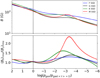 |
Fig. 1 Magnetic field characteristics. Top: horizontally averaged magnitude of the magnetic field. Bottom: horizontally averaged inclination of the magnetic field, defined as |

3 Results
3.1 Distribution of the magnetic fields
Figure 1 shows the horizontally averaged magnitude (top panel) and horizontally averaged inclination (bottom panel) of the magnetic field near the surface. All cases show a similar value of the magnetic field strength, except for the F star, which shows a somewhat higher value at and above the surface (marked by the dotted vertical line). The field inclination shows that the field becomes more horizontal for all cases higher up in the atmosphere. Between  , all cases show a peak in Bh/Bz, which probably corresponds to low-lying magnetic field loops. Higher up, Bh/Bz tends toward zero, in accordance with the upper boundary condition of a vertical field.
Table 1 lists the magnetic field characteristics for all cases for 〈τ〉 = 1 horizontal slice as well as for τ = 1 isosurface. We list the field magnitude  , the vertical field strength
  , the horizontal field strength
  , and the percent fraction of area occupied by kilogauss fields
  . The τ = 1 isosurface refers to the surface where τ = 1 for each vertical column in the 3D cube. The data points are calculated by interpolating logarithmically against the corresponding τ column to where τ = 1. Here, τ refers to the optical depth corresponding to a reference wavelength of 500 nm. The τ = 1 isosurface therefore provides an observational point of view for understanding the results. We also considered the horizontal slice because the thermodynamic stratification is expected to be quite uniform in the horizontal direction, allowing a better understanding of the physics of the magnetic field distribution. The columns show that for the horizontal slice, the average field strength is quite similar (100 to 130 G) for all cases, but the value increases significantly for the F star (almost 190 G) and G star (almost 130 G) when the τ = 1 isosurface is considered. For the other cases, the change is almost within the standard deviation and decreases with Teff. In addition, the area fraction of kG fields for the F star is about 0.8% for the τ = 1 surface, whereas for the 〈τ〉 = 1 horizontal slice, it is almost zero. We note here that this result arises because the field strength of the strongest fields corresponds to pressure equipartition (including the
  term) at this height, which is just about one kilogauss (kG); this result is discussed in detail in Sect. 4.1. For the other cases, the area fraction is roughly 0.5% either way.
Figure 2 shows the probability density function (PDF) of the magnitude of the magnetic field for the horizontal slice at 〈τ〉 = 1 (top panel) and for the τ = 1 isosurface (bottom panel). All stars show a rather similar distribution of the photospheric magnetic fields B, with most of the field between 20 to 100 G (slightly higher for the F star) and a more rapid drop-off (knee) in the kG regime. For the horizontal slice, the field strength for the kG knee shows an inverse trend with Teff. These kG fields mostly form in the downflow lanes (see Appendix B for separate PDFs of the magnetic field in upflows and downflows). The vertical dotted and dashed lines mark the field strength corresponding to equipartition with pgas (i.e., Beqp,gas) and  , respectively, for all the cases. We note that there seems to be a trend in the location of the kG knee and the equipartition field strength. We also note that when it is compared against gas pressure alone, the F star seems to have superequipartition fields. This tendency toward having superequipartition fields relative to pgas decreases toward later spectral types, in which the M star fields are decidedly subequipartition. We discuss this relation further in Sect. 4.1. Briefly, we expect the strongest fields to be situated in intergranular lanes, with the strength of the field being such that it balances the external pressure.
When the τ = 1 isosurface is considered (bottom panel), the field distribution is roughly similar and does not show the trend for kG fields from the 〈τ〉 = 1 slice. In addition, the field strengths for the F star are generally higher. For the fields that are concentrated by flux expulsion, that is, the fields that are in equipartition with the flows (about a few 100 G), this is due to a depression in the τ = 1 isosurface in the intergranular lanes. Because opacity in the photospheres of cool stars strongly depends on temperature, the τ = 1 surface generally dips below z〈τ〉 = 1 in the cooler intergranular lanes. For the kG fields, however, the dominant mechanism is evacuation of plasma in the flux tubes, causing τ = 1 to form deeper below and radiation to escape from lower levels. This depression in the optical depth is somewhat similar to the Wilson depression (WD; Wilson & Maskelyne 1774) of the optical surface in sunspots. Because the pressure increases through stratification and conservation of flux, the field strength is stronger deeper down. The magnitude of this depression scales with Teff as well as pressure scale height (Beeck et al. 2015), and it is the strongest for the F star and weakest for the M star. These results are consistent with simulations of weak stellar magnetism by Salhab et al. (2018), who also reported similar values of kG field concentrations for all cases, as well as the scaling of the Wilson depression with pressure scale height. The factors that affect the kG field distribution are discussed below in the context of convective collapse (Spruit 1979), and the pressure balance in individual flux concentrations is described in Sect. 4.1.
Characteristics of magnetic field near the surface for each stellar type.
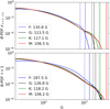 |
Fig. 2 PDF of the strength of magnetic field B for the SSD F (blue), G (black), K (green) and M star (red). Top: PDF of B calculated for the geometric surface z〈τ〉 = 1 corresponding to the height at which 〈τ〉 = 1. Bottom: same plot as the top, but for the iso τ = 1 surface. The vertical lines correspond to the pressure equipartition field |


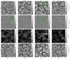 |
Fig. 3 Snapshots of the bolometric intensity I (in 1010 erg/cm2/s) for the SSD case (first row) and the corresponding vertical magnetic field B𝓏 (in kG; second row) and the horizontal magnetic field Bh (in kG; third row) at the iso τ = 1 surface for spectral types (from left to right) F, G, K and M. Snapshots of I for the HD case are plotted for comparison (last row). The color bars are identical for the SSD and HD cases. The green circles indicate magnetic bright points. |
3.2 Bolometric intensity
In Paper I we considered the changes in thermodynamic structure due to SSD-generated magnetic fields. We showed that these changes resulted in a decrease in density scale height Hρ, as well as in convective velocities near the stellar surface. Here, we consider how these changes affect the intensity structure.
The SSD magnetic fields affect the bolometric intensity Ibol in multiple ways. The evacuation of plasma through concentrated magnetic fields in intergranular lanes leads to the formation of bright points. This is generally attributed to the hot-wall effect (Spruit 1976), where the low-density plasma in the intergranular lanes is heated up by the surrounding hot dense upflows, which causes the former to appear bright. This effect is easily seen in the modeled F, G, K, and (to a lesser degree) M stars (see Fig. 3).
In addition, there are changes in the spatial distribution of Ibol due to the SSD. The top panel of Fig. 4 shows the magnitude of the spatial power spectra Pk of Ibol for all the HD and SSD cases (see Appendix A for details of how the power spectrum is calculated). We note that the spatial frequency was scaled by the box size, which essentially corresponds to a pressure scale height scaling (see Sect. 2.2 of Paper I for details). This ensures that all plots have the same range on the x-axis. The bottom panel shows the relative change in the power between the SSD and HD cases (Pk,SSD/ Pk,HD) – 1, with positive values corresponding to an increase in power in the SSD case.
The common interpretation of Pk, as calculated here, is in terms of the level of contrast at different spatial scales (Nordlund et al. 1997). We took the peaks of these spectra to be an indication of the granulation scales because the strongest contrast is expected at the granulation scale (bright granule centers vs. dark intergranular lanes). Because the granule sizes vary over a range of scales, we calculated the center of gravity (CG) over a range of k (marked by the gray shaded region) to estimate an average spatial wave number kCG that corresponds to an average granule size. The peaks of the power spectra lie between x0/x ∈ (4, 9). With that in mind, we restricted the limits for the CG calculation between x0/x ∈ (2, 20). For reference, this corresponds to a spatial frequency between 0.22 Mm−1 (or 4.5 Mm in length) and 2.2 Mm−1 (or 0.45 Mm in length) for the G star, where the typical granule size is ~ 1.5–2 Mm, corresponding to a spatial frequency of ~0.67 −0.5 Mm−1. The results are presented in Table 2. We interpret the positive change in kCG for all cases as an indication for a slight decrease in the average granule size for SSD cases (as x ~ 1/k), relative to the HD cases. The results indicate a positive δk (smaller scales) for granulation in the presence of an SSD compared to the HD case. A modification of the limits (k1 from 2 to 3 and k2 from 10 to 20) affects δk, but not its sign. The value of δk/kHD ranges from +1.1% to +3.8% for all the stellar types considered (M, K, G, and F) for k1 = 2 or 3 and k2 = 10, 15, or 20.
In Fig. 5, we plot the PDF of the bolometric intensity for all the SSD as well as HD cases. The F, G, and K stars show a clearly bimodal distribution, with the bright peak corresponding to mean granular intensities, and downflows corresponding to mean intergranular lanes intensities. This is consistent with the distributions obtained from a variety of other simulations of stellar photospheres (Beeck et al. 2012, 2013a; Magic et al. 2013; Salhab et al. 2018). The M star also has a somewhat bimodal distribution, but it is not as prominent as in the other cases because the contrast between granules and intergranular lanes is very low. All SSD cases show an extended bright tail (right side of the PDFs) that corresponds to the formation of magnetic bright points in intergranular lanes. In addition, the G and K stars show slight excess intensities in the bright flank (above the bright tail, corresponding to bright granules) for the SSD cases, whereas the F star shows a slight decrease. The F and G stars also show a steeper fall-off at the dark flank (left side of the PDFs), which contributes to a reduction in contrast for the SSD cases, as noted in Table 3.
The effect of SSD fields on intensity at subgranular scales is more varied for different spectral types. The bottom panel of Fig. 4 shows a prominent increase in power for the K star at the smallest spatial scales, corresponding to the high-contrast bright points present in the intergranular lanes. This is consistent with the bright tail in Fig. 5. A similar interpretation also holds for the G star. We also see bright points in the F star case (see the first column in Fig. 3). However, these bright points do not lead to an increase in power because the magnetic fields also restrict the convective velocities and act as an effective viscosity. This causes the flow to become more laminar and leads to granules with a smoother appearance, thus decreasing the amount of small-scale substructure and contrast. We caution against interpreting the results in the k > 100 range because the effects of numerical diffusion are non-negligible there.
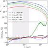 |
Fig. 4 Spatial power spectra Pk of bolometric intensity Ibol for the SSD (solid) and HD (dashed) cases plotted against spatial frequency 1/x (normalized by the horizontal box size x0 for each star). Top: Pk for all cases normalized by the SSD F star total power (Σk Pk). Bottom: Relative change in power at different scales between the SSD and HD cases. The gray shaded region refers to the approximate scales corresponding to the range in granule sizes, for which the center of gravity is calculated in Table 2. |

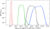 |
Fig. 5 PDF of the bolometric intensity for the SSD (solid) and HD (dashed). The vertical axis is given in semilog. |
3.3 Vertical velocity
In Paper I we showed a general reduction in vertical velocity υ𝓏 for SSD cases near the photosphere. Here, we examine the change in the distribution of υ𝓏 relative to the HD cases in more detail.
The top panel of Fig. 6 shows the PDF of υ𝓏 at the τ = 1 isosurface, normalized by (υ𝓏,rms)HD. This normalization allows us to compare the shapes of the PDF for the different stars and to examine the changes between the SSD and HD cases (Fig. 6, bottom panel). First of all, we note that all cases show a similar PDF, with a sharp high peak for upflows and a broad low peak for downflows. There are some exceptions to the general trend: The downflow peak for the M star is lower than for the others. This might partly be a consequence of a somewhat higher upflow fraction for the M star (~60%) compared to the other stars (~55– 57%). Another difference is the upflow peak for the F star, which is offset to relatively lower velocities than for the other stellar types. This is consistent with a thicker tail for the high-pflow velocities υ𝓏 and probably reflects the larger spread in υ𝓏 for the F star. Notwithstanding these small differences, the distribution of velocities is remarkably similar for all the four stars.
In the presence of SSD magnetic fields, the mean upflow velocities decrease. This might be a consequence of the reduced kinetic energy in upflows, which is due the SSD fields: The fields effectively enhance viscosity. The mean downflow velocities remain relatively unchanged. This may be related to the fact that magnetic fields in downflows are close to vertical, allowing downflowing plasma to remain relatively unhindered, whereas the magnetic field above granules is largely horizontal, which impedes upflowing plasma (Schüssler & Vogler 2008; Rempel 2014).
Average values for various quantities related to υ𝓏 and Ibol.
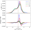 |
Fig. 6 Vertical velocity υ𝓏 at the iso τ = 1 surface normalized by the r.m.s vertical velocity in the HD case |


3.4 Spatial distribution of energy
The spatial power spectrum plot for the magnetic energy (ME) in Fig. 7 (top panel) shows a fairly similar distribution for the G, K, and M star, whereas for the F star, the spectrum is slightly steeper at the larger scales and has higher power than the spectra for other stars at all wave numbers. The power spectra for the kinetic energy (KE; middle panel) are also very similar for all the stars at smaller wave numbers and are roughly similar for the larger wave numbers. The relative changes in the KE power spectra between the SSD and the HD cases (bottom panel) are remarkably similar for all the models, with a decrease in energy at the largest scales (smallest wave numbers) and the smallest scales (largest wave numbers). On the other hand, there is no significant change in the power at scales roughly corresponding to granule sizes (see Sect. 3.2 for details of the granulation scales). Because the dimensions of all the stars are scaled to have a similar number of vertical pressure scale heights (and the horizontal size is scaled accordingly to maintain the aspect ratio), the similarity in all the power spectra points to a simple pressure scale height scaling of the relevant dynamics.
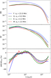 |
Fig. 7 Spatial power spectrum of magnetic and kinetic energies at the iso τ = 1 surface. Top: power spectrum of the magnetic energy for all the SSD cases. Middle: power spectrum of the kinetic energy for all the SSD (solid, dark) and HD (dashed, light) cases. Bottom: percent change in the kinetic energy power spectrum for SSD cases relative to HD cases. The top and middle plots are normalized by the total kinetic energy for the F star (solid blue). |
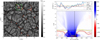 |
Fig. 8 Horizontal force balance in a vertical slice of a magnetic field concentration for the F star. Left: plot of the bolometric intensity. The selected magnetic element is highlighted by the green rectangle. The red contours represent areas with B2/8π > pgas. Right: map of Bɀ in the x-plane with the horizontal axis in Mm and the vertical axis in the number of pressure scale heights above (negative) and below (positive) the 〈τ〉 = 1 height. The dark red, red, and yellow contours show the iso log10 τ =1,0,−1 surfaces, respectively. The line plot on top shows the diagonal terms of the total stress tensor (see Eq. (1) and Sect. 4.1 for details). An animation is available online. |
4 Discussion
4.1 Kilogauss magnetic fields
As mentioned in the introduction, the distribution of small-scale magnetic field strengths is well studied for the solar case. The weak (sub-kG) field distribution is explained in terms of an equipartition between KE and ME: Weak turbulent magnetic fields are carried upward and outward from granule centers and are collected in intergranular lanes up to kinetic energy equipartition in a process called flux expulsion (Weiss 1966). However, the field strength corresponding to KE equipartition is substantially sub-kG. To explain the presence of kG fields, the convective collapse mechanism (Parker 1978; Spruit & Zweibel 1979; Spruit 1979) has usually been invoked. A qualitative picture of the mechanism is as follows: The magnetic field is accumulated in downflow lanes due to flux expulsion from the granule centers. This field can intensify up to equipartition with kinetic energy. At this point, a nascent flux tube forms. While plasma in the tube continues to flow downward, the flow of plasma into the lanes is restricted by the Lorentz force, which causes the tube to become evacuated. Finally, to maintain horizontal force balance, the tube is compressed, causing the magnetic field to amplify, potentially up to pressure equipartition (pmag = B2/8π ≈ pgas). The efficiency of this mechanism can be thought of in terms of the minimum plasma β = pgas/pmag (or the strongest fields) for which this instability can work in an idealized flux tube. Rajaguru et al. (2002) showed that this minimum β shows an increasing trend with Teff and decreasing 𝑔, implying that convective collapse is more efficient for hotter stars.
However, this mechanism can only explain the field strength up to pressure equipartition, whereas our simulations reveal superequipartition fields for the F and G stars. The reason for this is that convective collapse is an idealized model, which assumes that flux concentrations exist as stable thin vertical flux tubes and only accounts for the importance of magnetic pressure and gravity. Realistic simulations of flux concentrations have shown that the assumptions are not quite satisfied, especially near the surface where β ~ 1 (Yelles Chaouche et al. 2009).
Some idealized convection studies have indeed shown to result in magnetic field concentrations well above Beqp, for example, in Bushby et al. (2008), who cited dynamic pressure as a major factor leading to superequipartition fields. This becomes especially important for hotter stars such as our F star, where velocities in the photosphere are sonic on average and the turbulent pressure is non-negligible compared to gas pressure. To understand which factors are important for the formation and evolution of flux concentrations, we considered the momentum balance equation in the following form:
 (1)
(1)
Here, the indices i, j correspond to the x,y, ɀ directions and 𝑔i = (0,0, −𝑔surf). The terms on the right-hand side within the parentheses are the gas pressure, and when averaged over time, the Reynolds and Maxwell stresses. The Maxwell stresses themselves can be decomposed into an isotropic magnetic pressure term and a general magnetic tension term, respectively.
We considered individual field concentrations for the F star (Fig. 8) and the K star (Fig. 9). We note that Eq. (1) must always be satisfied at any given point of time. For the horizontal force balance, however, we only considered the diagonal terms (i = j) of the total stress tensor (first bracket on the right hand side) for simplicity. For a cut along the y-axis, these terms (gas pressure pgas, magnetic pressure B2/8π,  , and
, and  , plus the sum of all the components) are plotted for the highlighted field concentration in the left panel for Figs. 8 and 9 at a given instant.
If there were perfect horizontal pressure balance, the thick blue line in Figs. 8 and 9 would be flat. This is clearly not the case, however, even for the K star. This means that we possibly miss contributions from the time-dependent d(ρυi)/dt term, as well as from the off-diagonal components (i ≠ j in Eq. (1)) of the stress tensor. To account at least for the former term, we averaged over the lifetime of the magnetic field concentrations for the F and K star. The corresponding averages are plotted in Fig. 10. Fortunately, the horizontal balance is reasonably well maintained (i.e., the thick blue line is relatively flat) with just the diagonal components for the F star (top) as well as the K star (bottom). The difference between the two cases is the strength of the magnetic pressure relative to the gas pressure: In the F star, B2/8π > pgas in the center of the field concentration, whereas for the K star, B2/8π ~ pgas/3. The reason for this difference in this case is the additional contribution from the  term, which is roughly pgas/4 outside of the field concentration. We note that the value of Beqp,tot is about 1 kG for the F star for the ɀ〈τ〉 = 1 slice, which explains why the kG fraction in this case is essentially zero.
The degree of evacuation of a flux tube is dependent on the level of superadiabaticity (Spruit & Zweibel 1979). Hotter stars have higher superadiabaticity near the surface (Rajaguru et al. 2002; Beeck et al. 2013a). This explains the trend of kG fields in G, K, and M stars relative to pressure-equipartition field strength. However, based on the analysis above, for the F star, an additional contribution from the diagonal component of the Reynolds stresses (here,  ) must be accounted for at the very least. When this is done, the equipartition field strength rises to ~ 1 kG and the fraction of the field strength above this essentially drops to zero, as noted in Sect. 3.1. Moreover, the depth of the iso τ = 1 surface in terms of
  for the F star in the surface in the intergranular lane can be >
  , whereas for the K star, this dip is much less than
  . This explains why the PDFs for the iso τ = 1 surface look rather similar for all cases: The horizontal force balance is maintained relatively deeper down for hotter stars (we “see” stronger fields), whereas for cooler stars, the depth difference is not as significant.
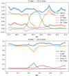 |
Fig. 10 Average over time of the line plots described in Fig. 8 (top) and Fig. 9 (bottom), respectively. The error bars are the 1σ- standard error. |
4.2 Granulation and intensity distribution
All models show slight changes in the apparent granulation when the SSD fields are included. In Paper I we showed that the inclusion of SSD fields results in a reduction in the ratio of horizontal to vertical velocities υh,rms / υɀ,rms, as well as in the density scale height Hρ. Above the surface, Hρ reduces for the SSD F star, but it remains largely the same for the SSD G, K, and M star because the decrease in turbulent pressure is roughly compensated for by an increase in magnetic pressure. However, υh,rms / υɀ,rms decreases for all cases. Based on simple momentum conservation arguments, the diameters of the convection cells at any depth are given by D ≈ 4(υh / υɀ)Hρ (Nordlund et al. 2009), so that we would expect the granule size to decrease accordingly. To verify this, we based the average granule size on the peak of the spatial power spectrum Pk of Ibol. Previous simulations have shown a tight correlation between granule diameters derived from this relation and Pk (Magic et al. 2013). A decrease in granule size would imply a shift to smaller spatial scales (higher spatial frequency) of the peak. This is, in fact, the case for all the stars, as shown in Table 2. This is also supported by observational indications of the relation between the magnetic field and granule size for the Sun. Various studies of variation in granule size within an active region (Title et al. 1992; Narayan & Scharmer 2010) and over the solar activity cycle (Ballot et al. 2021) showed a general inverse correlation between the granule size and the magnetic field strength.
At the smaller scales, the features are more varied in the spectral types. As mentioned before, all cases exhibit magnetic bright points in intergranular lanes. The relation between magnetic field concentrations and intensity is clearer in the joint histogram of Bz and the normalized intensity  and when the mean values of Î are plotted for each Bz bin (Fig. 11, top panel). The F, G, and K stars have quite similar mean Î values, with a correlation between bright features and strong Bz values that is qualitatively similar to observational findings for the Sun (Kahil et al. 2017). The trend is also similar for the M star, but the correlation is not as strong. The plots for F, G, and K star basically overlap because the intensity is normalized by σI. In addition, the horizontal fields Bh show no such correlation with intensity (Fig. 11, bottom panel), but firmly connects bright points to vertical field concentrations. This confirms the result found for the Sun by Riethmüller & Solanki (2017), for example.
Bright points are expected to enhance the power in the Ibol spatial power spectra at smaller scales, but this is clearly only the case for G and K stars. This can be understood in terms of the location in which the τ = 1 surface is formed with respect to the location in which the energy transfer shifts from convective to radiative (Nordlund & Dravins 1990) for different stellar types. As discussed in Sect. 4.2 of Paper I, for the F and G star, the τ = 1 layer forms below the location in which most of overturning of plasma takes place, leading to naked granules. For the K and M star, however, it forms above this location, leading to hidden granules (see also Sect. 3.2 of Beeck et al. 2013b) for a more comprehensive description of what constitutes a naked vs. hidden granule). Especially for the F star, the turbulent structures within the granules are seen very clearly in the HD case. However, with SSD fields, this turbulent appearance is significantly smoothed out because the magnetic field acts like an effective viscosity and hinders the flow. This affects not only the intensity distribution, but also the overall radiative flux: For the F star, the bolometric intensity decreases slightly (see Col. 4 of Table 3), that is the decrease in intensity due to the magnetic field’s effect on convection is stronger than the enhancement due to bright points. This effect is not as strong for the G and K star because the increase in contrast due to bright points dominates. In addition, the bolometric intensity increases slightly. For the M star, there is practically no change because bright points are relatively infrequent and their contrast is also relatively low.
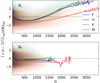 |
Fig. 11 Mean values of the normalized intensity |

4.3 Energy distribution and vertical velocities
Our simulations show remarkably similar spatial distributions of not just KE and ME, but also for the change in KE between SSD and HD simulations. Because all boxes are scaled by the number of pressure scale heights, this implies a simple pressure scale height proportionality between important scales in the considered stellar atmospheres. The SSD fields reduce the KE at subgranular scales and also reduce the scale of the whole box. The energy for the magnetic fields is extracted from the KE reservoir at small (subgranular) scales, which leads to fields with a strength near KE equipartition, and this ME cascades to the largest scales, resulting in a net reduction of the average KE. Global simulations of the SSD also show a similar reduction in KE at the largest scale (Hotta et al. 2022), which might indicate significant global consequences in stellar convection with SSD fields.
An observational signature associated with this reduction in convective velocities is the change in the convective blueshift of photospheric lines (Dravins et al. 1981). Convective blueshift is one of the few measurable quantities that encodes information about stellar granulation. A reduction in υz would imply shifts in the line profiles that are used to estimate the convective blueshift. We refrained from calculating line bisectors and so on because these simulations are gray, and these quantities are likely to be inaccurate. We plan to carry out this analysis in a subsequent paper in this series.
The reduction of KE at the smallest scales of about 40% (see the bottom panel of Fig. 7 near k~102) reflects the near-equipartition division of energy between KE and ME at the scales at which the field amplification takes place. The SSD mechanism and the corresponding scale-dependent transfer of energy between the KE and ME reservoirs has been extensively studied and was shown to be quite universal (Moll et al. 2011).
Another way to study the effect of SSD fields on the intensity is to consider the joint PDFs of Î and υz/(υz,rms)HD and to examine the difference between the mean Î for SSD and HD cases. In brief, we computed the mean value of the intensity in every velocity bin for the SSD and HD case and plot the difference in Fig. 12. For the F, G, and K star SSD cases, Î is enhanced in downflows, as expected from bright points forming in down-flows. Interestingly, Î slightly increases for upflows as well for all cases (except the F star), which could mean that granules are slightly brighter for SSD cases in general.
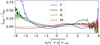 |
Fig. 12 Difference between the SSD and HD cases for the mean normalized intensity Î as a function of normalized vertical velocity υz/(υz,rms)HD at the iso τ = 1 surface. Positive values on the vertical axis mean a higher mean value for the intensity from the SSD case at the corresponding velocity bin. Positive values on the horizontal axis represent upflows. |
5 Conclusion
The SSD fields in our simulations affect the photosphere in a rather similar manner for the cool-star spectral types considered here: The fields are amplified due to turbulent plasma motions at subgranular spatial scales. These fields are then collected in intergranular lanes, where they are concentrated to kG levels while (roughly) maintaining horizontal force balance. For the F star, the horizontal force balance is satisfied only when Reynolds stresses are included, which causes the magnetic pressure to be higher than the gas pressure in the strongest flux concentrations. Magnetic bright points are also occasionally visible in the down-flow lanes, with a clear correlation of Bz with Î, as well as an increase in the bright tail of the intensity distribution. There is also an overall slight decrease in granule size. Because of the SSD fields, the upflow velocities also decrease, again with a similar signature in PDFs of υz/(υz,rms)HD for all cases. This decrease in upflow velocities signals a possible reduction in the expected convective blueshift. In summary, an SSD acting in stellar photospheres is expected to have an effect on spectral line shifts, limb darkening, and stellar variability at short timescales. We plan to investigate these possibilities in subsequent papers in this series.
Movies
Movie 1 associated with Fig. 8 (bright_pt_F_pres_x_cut) Access here
Movie 2 associated with Fig. 9 (bright_pt_K_pres_x_cut) Access here
Acknowledgements
We thank the anonymous referee for their comments and careful consideration, which significantly helped improve the presentation of this paper. T.B. is grateful for access to the supercomputer Cobra at Max Planck Computing and Data Facility (MPCDF), on which all the simulations were carried out. This project has received funding from the European Research Council (ERC) under the European Union’s Horizon 2020 research and innovation programme (grant agreement no. 695075).
Appendix A Spatial power spectrum
To compute the spatial power spectrum, we used the following procedure:
For a given 2D quantity q, take the 2D FFT (with the zero-frequency mode shifted to the center, e.g., with numpy.fft.fftshift in python using numpy) giving
 .
.Multiply
 with its complex conjugate
  to get
  .
.For each radial wave number
 , construct a one-pixel wide mask.
Take the mean of all the data in each mask and multiply by the radius of the mask to obtain the power Pk.
For the bolometric intensity, we used  . For the kinetic energy, we used
  . For the magnetic energy, we used
  .
.
Appendix B Additional plots
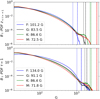 |
Fig. B.1 PDF of the magnitude of the magnetic field in upflows for the geometric surface z〈τ〉=1 (top) and for the τ = 1 isosurface (bottom). |
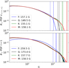 |
Fig. B.2 PDF of the magnitude of the magnetic field in downflows for the geometric surface z〈τ〉=1 (top) and for the τ = 1 isosurface (bottom). |
References
- Ballot, J., Roudier, T., Malherbe, J. M., & Frank, Z. 2021, A&A, 652, A103 [NASA ADS] [CrossRef] [EDP Sciences] [Google Scholar]
- Bastien, F. A., Stassun, K. G., Basri, G., & Pepper, J. 2013, Nature, 500, 427 [Google Scholar]
- Bastien, F. A., Stassun, K. G., Basri, G., & Pepper, J. 2016, ApJ, 818, 43 [NASA ADS] [CrossRef] [Google Scholar]
- Beeck, B., Collet, R., Steffen, M., et al. 2012, A&A, 539, A121 [NASA ADS] [CrossRef] [EDP Sciences] [Google Scholar]
- Beeck, B., Cameron, R. H., Reiners, A., & Schüssler, M. 2013a, A&A, 558, A48 [NASA ADS] [CrossRef] [EDP Sciences] [Google Scholar]
- Beeck, B., Cameron, R. H., Reiners, A., & Schüssler, M. 2013b, A&A, 558, A49 [NASA ADS] [CrossRef] [EDP Sciences] [Google Scholar]
- Beeck, B., Schüssler, M., Cameron, R. H., & Reiners, A. 2015, A&A, 581, A42 [NASA ADS] [CrossRef] [EDP Sciences] [Google Scholar]
- Bellot Rubio, L., & Orozco Suárez, D. 2019, Liv. Rev. Sol. Phys., 16, 1 [Google Scholar]
- Bhatia, T. S., Cameron, R. H., Solanki, S. K., et al. 2022, A&A, 663, A166 [NASA ADS] [CrossRef] [EDP Sciences] [Google Scholar]
- Brandenburg, A., & Subramanian, K. 2005, Phys. Rep., 417, 1 [NASA ADS] [CrossRef] [Google Scholar]
- Brandt, P. N., & Solanki, S. K. 1990, A&A, 231, 221 [NASA ADS] [Google Scholar]
- Bushby, P. J., Houghton, S. M., Proctor, M. R. E., & Weiss, N. O. 2008, MNRAS, 387, 698 [CrossRef] [Google Scholar]
- Charbonneau, P. 2014, ARA&A, 52, 251 [NASA ADS] [CrossRef] [Google Scholar]
- Crass, J., Gaudi, B. S., Leifer, S., et al. 2021, arXiv e-prints [arXiv:2107.14291] [Google Scholar]
- de Wijn, A. G., Stenflo, J. O., Solanki, S. K., & Tsuneta, S. 2009, Space Sci. Rev., 144, 275 [NASA ADS] [CrossRef] [Google Scholar]
- Dravins, D. 1987, A&A, 172, 200 [NASA ADS] [Google Scholar]
- Dravins, D., Lindegren, L., & Nordlund, A. 1981, A&A, 96, 345 [NASA ADS] [Google Scholar]
- Hotta, H., & Kusano, K. 2021, Nat. Astron., 5, 1100 [NASA ADS] [CrossRef] [Google Scholar]
- Hotta, H., Kusano, K., & Shimada, R. 2022, ApJ, 933, 199 [NASA ADS] [CrossRef] [Google Scholar]
- Kahil, F., Riethmüller, T. L., & Solanki, S. K. 2017, ApJS, 229, 12 [NASA ADS] [CrossRef] [Google Scholar]
- Magic, Z., Collet, R., Asplund, M., et al. 2013, A&A, 557, A26 [NASA ADS] [CrossRef] [EDP Sciences] [Google Scholar]
- Moll, R., Pietarila Graham, J., Pratt, J., et al. 2011, ApJ, 736, 36 [NASA ADS] [CrossRef] [Google Scholar]
- Narayan, G., & Scharmer, G. B. 2010, A&A, 524, A3 [NASA ADS] [CrossRef] [EDP Sciences] [Google Scholar]
- Nordlund, A., & Dravins, D. 1990, A&A, 228, 155 [Google Scholar]
- Nordlund, A., Spruit, H. C., Ludwig, H. G., & Trampedach, R. 1997, A&A, 328, 229 [NASA ADS] [Google Scholar]
- Nordlund, Å., Stein, R. F., & Asplund, M. 2009, Liv. Rev. Sol. Phys., 6, 2 [Google Scholar]
- Parker, E. N. 1978, ApJ, 221, 368 [NASA ADS] [CrossRef] [Google Scholar]
- Rajaguru, S. P., Kurucz, R. L., & Hasan, S. S. 2002, ApJ, 565, L101 [NASA ADS] [CrossRef] [Google Scholar]
- Rempel, M. 2014, ApJ, 789, 132 [Google Scholar]
- Riethmüller, T. L., & Solanki, S. K. 2017, A&A, 598, A123 [NASA ADS] [CrossRef] [EDP Sciences] [Google Scholar]
- Rimmele, T., & Marino, J. 2006, ApJ, 646, 593 [NASA ADS] [CrossRef] [Google Scholar]
- Salhab, R. G., Steiner, O., Berdyugina, S. V., et al. 2018, A&A, 614, A78 [NASA ADS] [CrossRef] [EDP Sciences] [Google Scholar]
- Sánchez Almeida, J., & Martinez González, M. 2011, ASP Conf. Ser., 437, 451 [Google Scholar]
- Schüssler, M., & Vögler, A. 2008, A&A, 481, L5 [NASA ADS] [CrossRef] [EDP Sciences] [Google Scholar]
- Shapiro, A. I., Solanki, S. K., Krivova, N. A., et al. 2017, Nat. Astron., 1, 612 [NASA ADS] [CrossRef] [Google Scholar]
- Shporer, A., & Brown, T. 2011, ApJ, 733, 30 [NASA ADS] [CrossRef] [Google Scholar]
- Solanki, S. K. 1993, Space Sci. Rev., 63, 1 [Google Scholar]
- Solanki, S. K. 2003, A&ARv, 11, 153 [Google Scholar]
- Spruit, H. C. 1976, Sol. Phys., 50, 269 [NASA ADS] [CrossRef] [Google Scholar]
- Spruit, H. C. 1979, Sol. Phys., 61, 363 [CrossRef] [Google Scholar]
- Spruit, H. C., & Zweibel, E. G. 1979, Sol. Phys., 62, 15 [NASA ADS] [CrossRef] [Google Scholar]
- Title, A. M., Topka, K. P., Tarbell, T. D., et al. 1992, ApJ, 393, 782 [NASA ADS] [CrossRef] [Google Scholar]
- Vögler, A., & Schüssler, M. 2007, A&A, 465, L43 [Google Scholar]
- Weiss, N. O. 1966, Proc. Roy. Soc. Lond. Ser. A, 293, 310 [NASA ADS] [CrossRef] [Google Scholar]
- Wilson, O. C. 1978, ApJ, 226, 379 [Google Scholar]
- Wilson, A., & Maskelyne, N. 1774, Philos. Trans. Roy. Soc. London Ser. I, 64, 1 [Google Scholar]
- Witzke, V., Duehnen, H. B., Shapiro, A. I., et al. 2023, A&A, 669, A157 [NASA ADS] [CrossRef] [EDP Sciences] [Google Scholar]
- Yelles Chaouche, L., Solanki, S. K., & Schüssler, M. 2009, A&A, 504, 595 [NASA ADS] [CrossRef] [EDP Sciences] [Google Scholar]
All Tables
All Figures
|
Fig. 1 Magnetic field characteristics. Top: horizontally averaged magnitude of the magnetic field. Bottom: horizontally averaged inclination of the magnetic field, defined as |
| In the text | |
|
Fig. 2 PDF of the strength of magnetic field B for the SSD F (blue), G (black), K (green) and M star (red). Top: PDF of B calculated for the geometric surface z〈τ〉 = 1 corresponding to the height at which 〈τ〉 = 1. Bottom: same plot as the top, but for the iso τ = 1 surface. The vertical lines correspond to the pressure equipartition field |
| In the text | |
|
Fig. 3 Snapshots of the bolometric intensity I (in 1010 erg/cm2/s) for the SSD case (first row) and the corresponding vertical magnetic field B𝓏 (in kG; second row) and the horizontal magnetic field Bh (in kG; third row) at the iso τ = 1 surface for spectral types (from left to right) F, G, K and M. Snapshots of I for the HD case are plotted for comparison (last row). The color bars are identical for the SSD and HD cases. The green circles indicate magnetic bright points. |
| In the text | |
|
Fig. 4 Spatial power spectra Pk of bolometric intensity Ibol for the SSD (solid) and HD (dashed) cases plotted against spatial frequency 1/x (normalized by the horizontal box size x0 for each star). Top: Pk for all cases normalized by the SSD F star total power (Σk Pk). Bottom: Relative change in power at different scales between the SSD and HD cases. The gray shaded region refers to the approximate scales corresponding to the range in granule sizes, for which the center of gravity is calculated in Table 2. |
| In the text | |
|
Fig. 5 PDF of the bolometric intensity for the SSD (solid) and HD (dashed). The vertical axis is given in semilog. |
| In the text | |
|
Fig. 6 Vertical velocity υ𝓏 at the iso τ = 1 surface normalized by the r.m.s vertical velocity in the HD case |
| In the text | |
|
Fig. 7 Spatial power spectrum of magnetic and kinetic energies at the iso τ = 1 surface. Top: power spectrum of the magnetic energy for all the SSD cases. Middle: power spectrum of the kinetic energy for all the SSD (solid, dark) and HD (dashed, light) cases. Bottom: percent change in the kinetic energy power spectrum for SSD cases relative to HD cases. The top and middle plots are normalized by the total kinetic energy for the F star (solid blue). |
| In the text | |
|
Fig. 8 Horizontal force balance in a vertical slice of a magnetic field concentration for the F star. Left: plot of the bolometric intensity. The selected magnetic element is highlighted by the green rectangle. The red contours represent areas with B2/8π > pgas. Right: map of Bɀ in the x-plane with the horizontal axis in Mm and the vertical axis in the number of pressure scale heights above (negative) and below (positive) the 〈τ〉 = 1 height. The dark red, red, and yellow contours show the iso log10 τ =1,0,−1 surfaces, respectively. The line plot on top shows the diagonal terms of the total stress tensor (see Eq. (1) and Sect. 4.1 for details). An animation is available online. |
| In the text | |
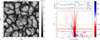 |
Fig. 9 Same as Fig. 8, but for the K star. An animation is available online. |
| In the text | |
|
Fig. 10 Average over time of the line plots described in Fig. 8 (top) and Fig. 9 (bottom), respectively. The error bars are the 1σ- standard error. |
| In the text | |
|
Fig. 11 Mean values of the normalized intensity |
| In the text | |
|
Fig. 12 Difference between the SSD and HD cases for the mean normalized intensity Î as a function of normalized vertical velocity υz/(υz,rms)HD at the iso τ = 1 surface. Positive values on the vertical axis mean a higher mean value for the intensity from the SSD case at the corresponding velocity bin. Positive values on the horizontal axis represent upflows. |
| In the text | |
|
Fig. B.1 PDF of the magnitude of the magnetic field in upflows for the geometric surface z〈τ〉=1 (top) and for the τ = 1 isosurface (bottom). |
| In the text | |
|
Fig. B.2 PDF of the magnitude of the magnetic field in downflows for the geometric surface z〈τ〉=1 (top) and for the τ = 1 isosurface (bottom). |
| In the text | |
Current usage metrics show cumulative count of Article Views (full-text article views including HTML views, PDF and ePub downloads, according to the available data) and Abstracts Views on Vision4Press platform.
Data correspond to usage on the plateform after 2015. The current usage metrics is available 48-96 hours after online publication and is updated daily on week days.
Initial download of the metrics may take a while.