| Issue |
A&A
Volume 689, September 2024
|
|
|---|---|---|
| Article Number | A198 | |
| Number of page(s) | 17 | |
| Section | Stellar atmospheres | |
| DOI | https://doi.org/10.1051/0004-6361/202449401 | |
| Published online | 13 September 2024 | |
Small-scale vortical motions in cool stellar atmospheres
1
Istituto ricerche solari Aldo e Cele Daccò (IRSOL), Faculty of Informatics, Università della Svizzera italiana,
6605
Locarno,
Switzerland
2
Euler Institute, Università della Svizzera italiana (USI),
6900
Lugano,
Switzerland
3
Kiepenheuer-Institut für Sonnenphysik (KIS),
Georges-Köhler-Allee 401a,
79110
Freiburg i.Br.,
Germany
Received:
30
January
2024
Accepted:
4
July
2024
Abstract
Context. Small-scale vortices in the solar atmosphere have received considerable attention in recent years. These events are considered potential conduits for the exchange of energy and mass between the solar atmospheric layers from the convective surface to the corona. Similar events may occur in the atmospheres of other stars and play a role in energy transfer within their atmospheres.
Aims. Our aim is to study the presence and properties of small-scale swirls in numerical simulations of the atmospheres of cool main-sequence stars. Our particular focus is on understanding the variations in these properties for different stellar types and their sensitivity to the surface magnetic field. Furthermore, we aim to investigate the role of these events in the energy transport within the simulated atmospheres.
Methods. We analyzed three-dimensional, radiative-magnetohydrodynamic, box-in-a-star, numerical simulations of four main-sequence stars of spectral types K8V, K2V, G2V, and F5V. These simulations include a surface small-scale dynamo responsible for amplifying an initially weak magnetic field. Thus, we can study models characterized by very weak, or, in near equipartition magnetic fields. To identify small-scale vortices in horizontal layers of the simulations, we employed the automated algorithm SWIRL.
Results. Small-scale swirls are abundant in the simulated atmospheres of all the investigated cool stars. The characteristics of these events appear to be influenced by the main properties of the stellar models and by the strength of the surface magnetic field. In addition, we identify signatures of torsional Alfvénic pulses associated with these swirls, which are responsible for a significant vertical Poynting flux in the middle photospheres of the simulated stellar models. Notably, this flux is particularly significant in the K8V model, suggesting that if ~70% of it is dissipated in the low chromosphere, small-scale vortical motions may play a role in the enhanced basal CaII H and K fluxes observed in the range of B − V color index 1.1 ≤ B − V ≤ 1.4. Finally, we present a simple analytical model, along with an accompanying scaling relation, to explain the peculiar result of the statistical analysis that the rotational period of surface vortices increases with the effective temperature of the stellar model.
Conclusions. Our study shows that small-scale vortical motions are not unique to the solar atmosphere and that their interplay with the stellar surface magnetic field may effect the observable chromospheric activity of main-sequence cool dwarf stars.
Key words: magnetohydrodynamics (MHD) / stars: atmospheres / stars: magnetic field
Corresponding author; This email address is being protected from spambots. You need JavaScript enabled to view it.
© The Authors 2024
 Open Access article, published by EDP Sciences, under the terms of the Creative Commons Attribution License (https://creativecommons.org/licenses/by/4.0), which permits unrestricted use, distribution, and reproduction in any medium, provided the original work is properly cited.
This article is published in open access under the Subscribe to Open model. This email address is being protected from spambots. You need JavaScript enabled to view it. to support open access publication.
1 Introduction
Given the ubiquitous presence of small-scale swirls in the solar atmosphere (see Tziotziou et al. 2023, for a review), it is reasonable to expect similar vortical flows in other stellar atmospheres. However, the unique properties of individual stars, such as the gravitational acceleration at the stellar surface, the effective temperature, and the mass density, may influence the properties of these small-scale features. In addition, magnetic fields play a crucial role in the generation and dynamics of swirls in the solar atmosphere as was demonstrated, for example, with simulations by Canivete Cuissa & Steiner (2020) or Battaglia et al. (2021). This suggests that the surface magnetic field of other stars are likewise important for stellar swirls (Wedemeyer et al. 2013). Specifically, magnetic fields appear to be tightly related to the transport of vortical motion and Poynting flux from the photosphere to the outer solar atmosphere within so-called magnetic tornadoes, which possibly contribute to the heating of the chromosphere or corona (Wedemeyer-Böhm et al. 2012).
The precise mechanism driving the upward transport of energy within magnetic tornadoes remains a topic of debate, with torsional Alfvénic pulses1 identified as the most probable candidate (Liu et al. 2019; Battaglia et al. 2021). In this scenario, small-scale swirls are the plasma counterparts to twist in the field lines of the vertically directed photospheric magnetic flux concentrations. These perturbations, originating in the surface layers of the atmosphere, can propagate upward along the flux tube into the chromosphere as pulses of torsional Alfvén waves. Moreover, numerical simulations indicate that about 80% of the swirls in the photosphere are consistent with this scenario (Canivete Cuissa & Steiner 2024).
Of incidental interest is the possible contribution of magnetic tornadoes to the chromospheric basal flux as a function of spectral type (Boro Saikia et al. 2018). Observations of main-sequence stellar populations reveal that stars with 1.1 ≤ B − V ≤ 1.4 exhibit a significantly enhanced chromospheric basal flux, the cause of which is not yet fully understood. Therefore we also studied the magnetic energy transported by these small-scale vortices and their potential to contribute to the chromospheric basal flux as a function of spectral type.
For this purpose, three-dimensional radiative-magnetohydrodynamic (R-MHD) box-in-a-star numerical models have been analyzed, specifically four main-sequence stellar models of spectral types K8V, K2V, G2V, and F5V. Originally, these simulations were performed to study the surface small-scale dynamo (SSD) in cool main-sequence stars by Riva et al. (2024). Thus, with these models at hand, it became possible to investigate the properties of vortices in the presence of a magnetic field that self-consistently emerges through an SSD action. We carried out a statistical analysis of the fundamental properties of the vortices during the saturation phases of the SSD and, for comparison with the quasi field-free case, the kinematic phases in different heights within the simulated atmosphere, and across different stellar models.
The paper is organized as follows: Sect. 2 describes the simulations and the vortex identification algorithm used in this study. In Sect. 3, we present results on the qualitative and quantitative properties of the vortices in the four stellar models. In addition, we introduce a simple analytical model for photospheric vortices that replicates one of the results of our statistical analysis. Finally, Sec. 4 provides a comprehensive summary and the conclusions.
2 Methods
2.1 Numerical simulations
The three-dimensional R-MHD simulations that serve as the basis of the present investigation have been carried out with the CO5BOLD code (Freytag et al. 2012) in the so-called box-in-a-star setup. This corresponds to simulating a small partial volume near the optical surface of a star, encompassing the layers where energy transport changes from predominantly convective to purely radiative. A constant and vertical gravitational acceleration is applied. The simulations use the long-characteristic radiative transfer module of CO5BOLD with Rosseland mean opacities and the diffusion approximation in the regime of high optical depths (log τR ≳ 2). Details on the numerical setup can be found in Riva et al. (2024).
The stellar models are primarily distinguished by their effective temperature, Teff, gravitational acceleration, g, and the chemical composition (metallicity), which here is taken to be the solar one. We note that the metallicity can have a noticeable impact on stratification, turbulence properties, and the operation of the SSD (e.g., Magic et al. 2013; Witzke et al. 2023). The study of its impact on small-scale swirls would require a model grid of varying metallicity, which is outside the scope of the present paper and left for future research. The main parameters g and the average Teff of the models are provided in the top set of rows in Table 1 together with the average pressure scale height at the surface of the model, Hp(z = 0). Here, surface denotes the space and time averaged optical depth surface τR = 1, which is also taken as the origin of the geometrical z-scale, z = 0. The surface gravity g was chosen to be that of a dwarf star placed on the main sequence.
The middle set of rows of Table 1 specifies the horizontal and vertical sizes of the simulated domains, Lx, Ly, and Lz, along with the grid spacing, indicated by Δx, Δy, and Δz. The vertical extension, Lz, was chosen such that the bottom boundary is at a depth where the entropy of the downflowing plasma approaches the essentially constant entropy of the upflowing plasma (see, Salhab et al. 2018, Fig. 11), whereas the top boundary is located well above the entropy minimum in the photosphere. The height extents of the computational domains, below and above the average Rosseland optical depth unity, are also displayed in this section of the table. Also given is the average size of a granule, Lgran, which was computed as the integral length scale of the vertical velocity spectrum according to Eq. (5) of Riva et al. (2024). The horizontal extent was specifically chosen to encompass approximately six granular scales within the computational domain. Vertically, the simulation domains extend from the near surface layers of the convective zone to beyond the entropy minimum of the photosphere, corresponding to approximately the top layers of the photosphere.
Preexisting and relaxed purely hydrodynamic simulations were seeded with a vertical magnetic field of Bz = 1 mG. These simulations were then further evolved and underwent a kinematic phase in which the seed magnetic field was exponentially amplified by the action of a subsurface SSD until it reached saturation. The bottom set of rows indicates the number of analyzed snapshots during the kinematic and saturated phases, Nkin and Nsat, respectively. The selection of snapshots for the kinematic and saturated phases was based on the mean ratio between kinetic and magnetic energy densities in the convection zone, ⟨Ekin/Emag⟩conv. We consider a time instance to be in the kinematic phase when ⟨Ekin/Emag⟩conv < 2.5 × 10⁻³, while saturation2 is defined when ⟨Ekin/Emag⟩conv > 2.5 × 10⁻².
Parameters describing the four simulated stellar models.
2.2 Identification algorithm
We employ the method proposed by Canivete Cuissa & Steiner (2022, 2024) to identify swirls in numerical simulations. This method accurately estimates the coordinates of the center of rotation, that is, the estimated vortex centers (EVC), for each fluid particle (grid cell) that exhibits some degree of curvature in the instantaneous velocity field. Since vortices can be viewed as groups of fluid particles coherently rotating about a common axis of rotation (Lugt 1979), clusters of EVCs form in the neighborhood of the core of a vortex structure. Therefore, the method uses clusters of EVCs to identify vortices. In this respect, the EVC method can be seen as a more accurate version of the curvature center method proposed by Sadarjoen & Post (1999), since it uses the velocity field and its derivatives to extract more detailed information about the curvature of the flow.
The accuracy of the method hinges on an accurate estimate of the radius of curvature and radial direction of the local flow. This requires the measurement of the rigid-body rotational component of the flow. Traditional methods have used mathematical quantities such as vorticity or swirling strength (Zhou et al. 1999) for this purpose, but Canivete Cuissa & Steiner (2022) showed that the optimal quantity is the Rortex criterion R (Tian et al. 2018; Wang et al. 2019). This advanced mathematical criterion measures alone the rigid body rotational component of a rotating flow and can be computed as
![Mathematical equation: $\[R=\omega \cdot \boldsymbol{u}_{\mathrm{r}}-\sqrt{\left(\omega \cdot \boldsymbol{u}_{\mathrm{r}}\right)^2-\lambda^2},\]$](/articles/aa/full_html/2024/09/aa49401-24/aa49401-24-eq1.png) (1)
(1)
where ω is the vorticity vector, ur is the normalized, real eigenvector of the Jacobian of the velocity vector, and λ is the swirling strength criterion, which formally is twice the imaginary part of the complex conjugated eigenvalues of the Jacobian of the velocity vector. For more details on these quantities, the reader can refer to Canivete Cuissa & Steiner (2020, 2022).
Clusters of EVCs can in principle be identified by eye. However, Canivete Cuissa & Steiner (2022) adapted the algorithm named clustering by fast search and find of density peaks (CFSFDP, Rodriguez & Laio 2014) to automate the process and reduce human bias in the identification. In addition, the proposed algorithm includes a cleaning procedure to remove misidentifications caused by noise or coherent but non-spiraling curved flows.
The algorithm outputs a list of identified vortices, each characterized by its center coordinates, the region it occupies in a horizontal section (in grid-cells), and its rotation direction (clockwise or counterclockwise). To quantify the effective radius of the swirl, reff, the following formula is employed,
![Mathematical equation: $\[r_{\mathrm{eff}}=\sqrt{\frac{N_{\mathrm{c}}}{\pi}} \Delta x,\]$](/articles/aa/full_html/2024/09/aa49401-24/aa49401-24-eq2.png) (2)
(2)
where Nc represents the number of grid cells occupied by the swirl and Δx is the grid spacing. Additionally, meaningful properties can be computed by combining this information with the values of physical variables on the swirl surface. For instance, the effective period of rotation, Peff, can be estimated using
![Mathematical equation: $\[P_{\text {eff }}=\frac{4 \pi}{\left\langle R_z\right\rangle_{\text {swirl }}},\]$](/articles/aa/full_html/2024/09/aa49401-24/aa49401-24-eq3.png) (3)
(3)
where ⟨·⟩swirl denotes the spatial average over the swirl surface, and Rz represents the vertical component of the Rortex vector, R = Rur. Another noteworthy property is the effective plasma rotational velocity, vϕ,eff, determined by
![Mathematical equation: $\[v_{\phi, \mathrm{eff}}=\frac{2 \pi r_{\mathrm{eff}}}{P_{\mathrm{eff}}}.\]$](/articles/aa/full_html/2024/09/aa49401-24/aa49401-24-eq4.png) (4)
(4)
A Python implementation of the resulting algorithm is open source on GitHub3 and named SWirl Identification by Rotationcenters Localization (SWIRL, Canivete Cuissa 2022). For more details on the method, the clustering algorithm, and the test cases, the reader can refer to Canivete Cuissa & Steiner (2022).
3 Results and discussion
In this section, we present and discuss the results of our analysis of the properties of the swirls in the simulated stellar atmospheres. First, we qualitatively validate the vortex identification algorithm, SWIRL, by comparing its output with emerging bolometric intensity maps and horizontal velocity fields. We then perform a comprehensive statistical analysis of the swirls properties, exploring their tight relationship with magnetic fields and study their energetics. Finally, we present a simple model of a photospheric vortex that supports a surprising result revealed by the statistical analysis.
3.1 Qualitative validation of SWIRL
Figure 1 shows the emerging bolometric intensity, Ibol, at a specific time during the kinematic phase for the four stellar models. At this time, the magnetic field remains relatively weak and exerts only a feeble influence on the flow dynamics. The granulation, characterized by cells of bright (warm) upflowing plasma surrounded by dark (cool) downflow into the intergranular space, is clearly visible in all models. In particular, the granules in the cooler stars (K8V and K2V) exhibit a smoother surface compared to the more vigorous dynamics visible in the G2V and F5V models.
From the horizontal velocity field at the surface (z = 0 km) and at the corresponding specific times, the SWIRL algorithm identifies the vortices shown in the four panels of Fig. 1. Each identified vortex is represented by a circle of size reff, denoting the effective radius of the vortex, and color-coded according to the direction of rotation (clockwise or counterclockwise). In Fig. 2, the identified vortices, accompanied by instantaneous streamlines of the horizontal velocity field, are shown in detail in two zoomed regions for the K8V and the F5V model.
The majority of the vortices are located within intergranular lanes, consistent with the results reported for simulations (Canivete Cuissa & Steiner 2024) and observations (Bonet et al. 2008) of the solar photosphere. This behavior is expected due to the conservation of angular momentum in intergranular downflows (Nordlund 1985; Wedemeyer & Steiner 2014). An examination of the instantaneous streamlines in the zoomed plots of Fig. 2 shows that the SWIRL algorithm consistently identifies vortical patterns in the velocity field. This is true regardless of whether the flow appears more laminar-like, as in the K8V model, or more vigorous and highly turbulent, as in the F5V model.
In Fig. 1, it can be seen that certain swirls, though not all, exhibit increased radiative intensity compared to their surroundings. An illustration of such a case is in the left panel of the Fig. 2 located at (x, y) = (1.10, 0.25) Mm. For comparison, in Appendix A we provide plots of the plasma mass density ρ at z = 0 km in the same time instances as shown in Figs. 1 and 2. We notice that areas of enhanced bolometric intensity in the integranular space that are associated with swirling motions exhibit significantly reduced mass densities, as is particularly well visible in Fig. A.2. Partial evacuation and enhanced radiative intensity in connection with swirling motions are the characteristic ingredients of so called nonmagnetic bright points. Nonmagnetic bright points occurring in magnetic field free simulations of the solar atmosphere have been investigated by Calvo et al. (2016). Here, they frequently occur under weak magnetic conditions in the kinematic phase of all stellar models.
In the saturation phase of the SSD, the qualitative behavior of the swirls in the bolometric intensity maps, and the reliability of their detection with the SWIRL algorithm carries over from the kinematic phase, as illustrated for the K8V model in Appendix B. The primary differences lie in the increased prevalence of bright features within intergranular regions, attributed to magnetic flux concentrations (see, Riva et al. 2024, Fig. 2) that appear to correlate with the presence of vortices, and the different number of swirls per granule. These aspects are quantitatively investigated in Sect. 3.2.
 |
Fig. 1 Emerging bolometric intensity, Ibol, for the K8V, K2V, G2V, and F5V models during the kinematic phase. Clockwise and counterclockwise vortices in the horizontal plane at z = 0 identified by the SWIRL algorithm are indicated by pink and green disks, respectively. The blue squares in the K8V and F5V panels mark the boundaries of the zoomed plots shown in Fig. 2. |
 |
Fig. 2 Identified swirls in the areas marked in blue in Fig. 1 for the K8V and F5V models. Clockwise and counterclockwise vortices identified by the SWIRL algorithm are indicated by pink and green disks, respectively. The horizontal component of the velocity field is represented by blue instantaneous streamlines. |
Location of the selected horizontal planes for the statistical analysis.
3.2 Statistical analysis
In this subsection, we examine the characteristics of the vortices identified by the SWIRL algorithm in both the kinematic and saturated phases. The number of snapshots analyzed in each regime for each stellar model is detailed in the bottom set of rows of Table 1.
Our analysis refers to four different heights in the simulated atmospheres, roughly corresponding to the surface layer of the convection zone, the stellar surface, the middle photosphere, and the high photosphere. The specific location is determined by the quantity ln(p0/p), where p0 is the horizontally averaged pressure at the mean optical depth τR = 1 (z ≈ 0 km), and p is the horizontally averaged pressure at the targeted plane. Table 2 gives the assumed values of ln(p0/p) along with the corresponding heights z in the simulation domains of the four models.
3.2.1 Surface distributions
To further investigate the distribution of vortices with respect to the granular configuration, Fig. 3 shows the bivariate distribution of the bolometric intensity Ibol and the absolute vertical magnetic field |Bz| for all the swirls identified at z = 0 km. The values of Ibol and |Bz| are taken at the center of each swirl. Moreover, we distinguish swirls identified during the kinematic phase (blue) from swirls in the saturated phase (orange) of the subsurface SSD.
The vertical dotted lines in Fig. 3 denote the mean bolometric intensity in the intergranular and granular regions for the four stellar models. These regions are defined based on the vertical velocity of the plasma, vz, at the surface (z = 0 km). Specifically, grid cells within the intergranular and granular regions satisfy the conditions vz < −σv,z and vz > σv,z, respectively, where σv,z is the standard deviation of the distribution of vz at z = 0 km. We note that the mean bolometric intensity in the intergranular and granular regions, as well as the difference between these two quantities, increase with increasing Teff. This is expected, as discussed for example in Beeck et al. (2011), Salhab et al. (2018), and Riva et al. (2024).
During the kinematic phase (blue), the majority of the swirls in all models are located in regions of low bolometric intensity, corresponding to intergranular lanes (that is, the maximum of the bivariate distribution is close to the left dotted line for all models). This finding confirms the visual impression conveyed by Fig. 1. The high end tails of the four distributions extend into the range of average granular bolometric intensity, indicating the presence of swirls associated with nonmagnetic bright points (e.g., see left panel of Fig. 2) or with granules4. Moreover, as the magnetic field is amplified by the subsurface SSD starting from an initial value of 1 mG, the bivariate distributions (still in the kinematic phase) span several orders of magnitude in |Bz|, that is 10−4 G ≲ |Bz| ≲ 102 G.
In the saturated phase (red), the distributions in Ibol remain centered around the intergranular bolometric intensities for the four models. At the same time, the distributions of | Bz| become narrower compared to the kinematic phase and shift to higher values (1 G ≲ |Bz| ≲ 104 G) due to stronger magnetic fields in the saturation phase. A notable feature emerges in all panels: the bivariate distributions exhibit the distinct presence of swirls in regions of high Ibol and near max(|Bz|), particularly evident in the K2V and G2V models. This means that there exist bright, strongly magnetized swirls, suggesting the presence of swirls associated with magnetic bright features (MBFs), a phenomenon previously documented in both solar observations (see, e.g., Bonet et al. 2008) and simulations (see, e.g., Moll et al. 2011), and also discussed in detail in Appendix B. Notably, the red boxes in the top-right corners of the four panels indicate the identification range for MBFs, as defined in Riva et al. (2024, Appendix B).
 |
Fig. 3 Bivariate distribution of the bolometric intensity Ibol and the absolute vertical magnetic field |Bz| in the center of the swirls identified on the surface layer at z = 0 km of the four stellar models. The distributions during the kinematic and saturation phases are shown in blue and orange, respectively. The vertical black dotted lines indicate the mean bolometric intensity in the intergranular (lower value) and granular (higher value) regions. The red shaded area indicates the identification range of magnetic bright feature (MBF) as defined by Riva et al. (2024). |
3.2.2 Physical properties
Next, we investigate the main physical characteristics of swirls across the four stellar models, the four heights in the simulation domain, and the two phases of the subsurface SSD, the saturation phase and, for comparison, the kinematic phase. We note that it is finally the saturation phase that corresponds to the observable states of the stellar atmospheres, but we compare with the kinematic phase to highlight the impact of the magnetic field on the statistical properties of small-scale swirls.
The physical properties we are interested in are: the average number of swirls per granule, the average ratio between the effective radius and the pressure scale height at z = 0 km, reff /Hp, the average effective period of rotation Peff, and the average rotational velocity vϕ,eff. The approximate size of the granules and pressure scale heights at z = 0 km for the four models are given in Table 1, while for computing reff, Peff, and vϕ,eff we employ Eqs. (2), (3), and (4), respectively.
The results of the statistical analysis are shown in Fig. 4. The top panel displays the number of vortices per granule in all four models, computed as the total number of vortices in the corresponding horizontal plane divided by the area of this plane, Lx · Ly, times the approximate area of a granule ![Mathematical equation: $\[L_{\text {gran }}^2\]$](/articles/aa/full_html/2024/09/aa49401-24/aa49401-24-eq5.png) . The number of vortices per granule gradually decreases as we ascend from the convection zone to the middle photosphere during both the saturation and the kinematic phases. These results are consistent with simulations of the solar atmosphere (see Moll et al. 2012; Canivete Cuissa & Steiner 2024). The prevalence of highly turbulent convective flows in the subsurface layers of cool stars naturally leads to the formation of vortex motions that explain the observed trend.
. The number of vortices per granule gradually decreases as we ascend from the convection zone to the middle photosphere during both the saturation and the kinematic phases. These results are consistent with simulations of the solar atmosphere (see Moll et al. 2012; Canivete Cuissa & Steiner 2024). The prevalence of highly turbulent convective flows in the subsurface layers of cool stars naturally leads to the formation of vortex motions that explain the observed trend.
Within the convection zone, the coolest model, K8V, has the lowest number of vortices, while this number increases with increasing Teff, in particular in the saturation phase. We ascribe this trend to the more vigorous plasma dynamics with increasing effective temperature. Conversely to the convection zone, we do not see any clear trend with Teff in the other layers. The only notable exception is the F5V model in the kinematic phase, which shows an exceptional high number of vortices in the high photosphere. This can be attributed to the energetic nature of the flows observed in the F5V model, which leads us to expect the presence of shocks already in the photosphere. These shocks could serve as a source of vortex motions in the upper atmospheres, especially in the virtual absence of magnetic fields, as it is the case for the kinematic phase (Moll et al. 2012).
The comparison between the kinematic and the saturation phases (round and square symbols, respectively) provides useful information on the impact of the magnetic field on the vortical plasma motion in the saturation phase. In particular, the presence of strong magnetic fields leads to a significant suppression of vortex formation in the lower layers, particularly in the convection zone. This suppression results from the “stiffening” effect of magnetic fields on the plasma as it approaches equipartition – a phenomenon known as magnetic quenching (see, e.g., Brandenburg & Subramanian 2005). In contrast, the number of vortices in the high photosphere increases by a factor of about 3–4 from the kinematic to the saturation phase, except for the F5V model where the increase is less distinctive. This observation underscores the central role of magnetic fields in the generation and dynamics of vortex features in the upper atmosphere in the saturation phase, where the magnetic field starts to locally dominate the plasma (small plasma-β = pgas/pmag).
This also suggests the existence of two distinct populations of vortices: surface swirls that arise from intergranular turbulence and magnetic flux concentrations, and vortices in the high photosphere that form due to magnetic tension and magnetic baroclinic forces (Canivete Cuissa & Steiner 2020). We thus conjecture that the lower abundance of swirls during the saturation phase in the middle photosphere compared to the other regions is due to two trends. On the one hand, convective turbulence declines with height in the atmosphere, playing a marginal role at the middle photosphere, and on the other hand are the plasma-β conditions not yet favorable for the generation of chromospheric-like swirls as they start to be in the high photosphere. The results are consistent with simulations of the solar atmosphere performed by Moll et al. (2012) and Battaglia et al. (2021). Moreover, the similar number of vortices in the high photosphere across models indicates that magnetic effects outweigh shocks in the formation of vortices within the magnetized upper photosphere, in agreement with the conclusions presented in Canivete Cuissa & Steiner (2020).
However, not all of the swirls occurring in the high photosphere can be due to coherent swirl structures that reach from the surface to the high photosphere as these are only a fraction of the swirls visible at the surface. We surmise that a significant fraction of these swirls are generated through local perturbations of the magnetic field, which may still originate from deeper layers but not necessarily in the form of swirls. For example, a small indentation in the boundary surface of a magnetic flux concentration can induce vortical motion further out in the atmosphere.
The second panel of the Fig. 4 shows the mean ratio between the effective radius of the swirl, reff, and the pressure scale height at z = 0 km, Hp. This ratio allows for a more meaningful comparison of results between different models than taking reff alone, as it takes the different scales inherent in each simulation into account. In stars characterized by larger granules, such as the F5V model, one would expect the swirls to be larger due to the larger scales of the flows. Therefore, by normalizing the radius by the surface pressure scale height – an essential length scale in the models – we obtain a normalized radius that allows for a more adequate comparison between the different models. The results show minimal variation in the mean normalized radius of vortices across spectral types, model layers, and magnetic field strengths, with values around reff/Hp ~ 0.25. Notably, the only discernible trend indicates a subtle increase in the photosphere. This result is consistent with the statistical analysis of the simulated solar atmosphere presented in Canivete Cuissa & Steiner (2024). The result suggests an intrinsic relationship between the average size of the swirls and the typical length scale of the simulated atmosphere. Given that the pressure scale height is related to the characteristic size of granular flows (see Table 1), this relationship seems reasonable.
The bottom two panels of Fig. 4 show the average rotational period, Peff, and the rotational velocity, vϕ,eff, of the swirls. An interesting observation is the correlation between the rotational velocity and the effective temperature of the stellar model at all heights. This correlation is expected, since higher effective temperatures generally correspond to higher plasma velocities. However, in contrast to this, we also observe the counterintuitive result that the rotational period also increases. Obviously, the increasing length scale with increasing effective temperature compensates for the higher plasma velocity. Predicting which effect dominates is not trivial. We further explore this intriguing finding with a simple analytical model in Sect. 3.3.
In the saturation phase of the SSD, a noticeable trend emerges: swirls in the subsurface and surface layers of the simulated atmospheres show slower rotation than in the kinematic phase. This phenomenon can be attributed to the conversion of turbulent kinetic energy into magnetic energy by the SSD, resulting in a deceleration of the rotation of vortices generated by turbulent convective plasma. However, an interesting contrast occurs in the high photosphere, where vortices tend to rotate faster in the saturation phase of the SSD. We attribute this effect to the presence of magnetic flux tubes that interconnect the different layers of the stellar atmospheres (see Appendix B), thus increasing the dependency of local properties of swirls among different layers. For example, the vertical gradient of the rotational period and velocity is very small between the middle and high atmosphere in the saturation phase, in contrast to the continuously declining trend in the kinematic case.
 |
Fig. 4 Properties of the swirls during the kinematic and saturation phases of the SSD and at different heights in the atmosphere of the four stellar models. The average number of swirls per granule in the simulation domain (top), the average ratio between radius and pressure scale height, reff/Hp (middle-top), rotational period, Peff (middle-bottom), and plasma rotational velocity vϕ,eff (bottom), are shown. The heights of the cross sections labeled as convection zone, surface, middle photosphere, and higher photosphere are given in Table 2 for the four stellar models. |
3.2.3 Alfvénic properties
Sections 3.2.1 and 3.2.2 underscore the fundamental role played by magnetic fields in shaping the properties of the swirls in the four models of stellar photospheres in the saturation phase of the SSD. Therefore, the goal of this subsection is to investigate this relationship in more detail. Of particular interest is the possible association of swirls in magnetized regions with torsional Alfvénic pulses (see, e.g., Wedemeyer-Böhm et al. 2012; Liu et al. 2019; Battaglia et al. 2021). These pulses provide a mechanism for energy transport from the surface atmospheric layer to the chromosphere and above.
Canivete Cuissa & Steiner (2024) conducted a thorough analysis of the swirl properties identified in simulations of the solar atmosphere. Their investigation focused on the imprints of torsional Alfvénic waves in atmospheric swirls, showing that about 80% of photospheric swirls are consistent with the scenario of a torsional Alfvénic pulse. However, these solar simulations started with a vertical magnetic field of a flux density of 50 G. Next, we reproduce part of this analysis for the four stellar models that feature an SSD generated magnetic field.
We begin by considering an incompressible plasma in magneto-hydrostatic equilibrium within the ideal MHD approximation. Then, for a torsional Alfvén wave propagating in the vertical direction along a vertically oriented magnetic field B = Bzez, the dispersion relation of the wave results in,
![Mathematical equation: $\[\boldsymbol{v}^{\prime}=-\frac{v_{\mathrm{A}}}{B_z} \boldsymbol{b}^{\prime},\]$](/articles/aa/full_html/2024/09/aa49401-24/aa49401-24-eq6.png) (5)
(5)
where v′ and b′ denote plasma velocity and magnetic field perturbations in the horizontal plane, respectively, while ![Mathematical equation: $\[v_{\mathrm{A}}=|\boldsymbol{B}| / ~\sqrt{4 \pi \rho} \geq 0\]$](/articles/aa/full_html/2024/09/aa49401-24/aa49401-24-eq8.png) is the local Alfvén speed. A detailed derivation can be found in Priest (2014, Sect. 4.3.1).
is the local Alfvén speed. A detailed derivation can be found in Priest (2014, Sect. 4.3.1).
From Eq. (5), we deduce that the perturbations v′ and b′ are either parallel or antiparallel, depending on the polarity of the vertical magnetic field, determined by the sign of Bz. Furthermore, assuming that the velocity perturbation manifests itself as a vortex, that is a rotational motion of the plasma in the horizontal plane, the magnetic field perturbation corresponds to the horizontal component of a twist in the predominantly vertically oriented magnetic field lines.
To quantify the horizontal velocity perturbations in the plasma, v′, we use the vertical component of the Rortex vector, Rz. Similarly, we define the magnetic Rortex vector, RB, which measures the equivalent to the rigid-body rotational component for the torsional component of the magnetic field. The magnetic Rortex vector is defined as the Rortex vector, Eq. (1), but with the magnetic field B as the input field, resulting in,
![Mathematical equation: $\[\boldsymbol{R}^{\mathrm{B}}=\tilde{\boldsymbol{J}} \cdot \boldsymbol{u}_{\mathrm{r}}^{\mathrm{B}}-\sqrt{\left(\tilde{\boldsymbol{J}} \cdot \boldsymbol{u}_{\mathrm{r}}^{\mathrm{B}}\right)^2-\left(\lambda^{\mathrm{B}}\right)^2},\]$](/articles/aa/full_html/2024/09/aa49401-24/aa49401-24-eq9.png) (6)
(6)
where ![Mathematical equation: $\[\boldsymbol{\tilde{J}=\nabla \times B}\]$](/articles/aa/full_html/2024/09/aa49401-24/aa49401-24-eq10.png) is proportional to the current density,
is proportional to the current density, ![Mathematical equation: $\[\boldsymbol{u}_{\mathrm{r}}^{\mathrm{B}}\]$](/articles/aa/full_html/2024/09/aa49401-24/aa49401-24-eq11.png) is the normalized, real eigenvector of the Jacobian of the magnetic field, and λB is the magnetic swirling strength (Battaglia et al. 2021).
is the normalized, real eigenvector of the Jacobian of the magnetic field, and λB is the magnetic swirling strength (Battaglia et al. 2021).
Using the vertical components of the Rortex and magnetic Rortex vectors, Rz and ![Mathematical equation: $\[R_z^{\mathrm{B}}\]$](/articles/aa/full_html/2024/09/aa49401-24/aa49401-24-eq12.png) , as proxies to quantify the perturbations associated with upward propagating torsional Alfvénic pulses, we can express Eq. (5) as,
, as proxies to quantify the perturbations associated with upward propagating torsional Alfvénic pulses, we can express Eq. (5) as,
![Mathematical equation: $\[\operatorname{sign}\left(R_z R_z^{\mathrm{B}}\right)=-\operatorname{sign}\left(B_z\right).\]$](/articles/aa/full_html/2024/09/aa49401-24/aa49401-24-eq13.png) (7)
(7)
This equation can be used to detect imprints of torsional Alfvénic pulses in the identified swirls of the stellar models. As we are interested in events that potentially transport energy from the photosphere into the upper atmosphere, our analysis targets the lower and upper photospheric layers of the simulations during the saturation phase of the SSD.
Figure 5 shows the bivariate distribution of the average Rz and ![Mathematical equation: $\[R_z^{\mathrm{B}}\]$](/articles/aa/full_html/2024/09/aa49401-24/aa49401-24-eq14.png) for swirls identified in the middle photosphere of the four stellar models during the saturated phase of the SSD. The averages are computed over the area of each swirl, and the color indicates the polarity and strength of the vertical component of the magnetic field in which the swirl is embedded.
for swirls identified in the middle photosphere of the four stellar models during the saturated phase of the SSD. The averages are computed over the area of each swirl, and the color indicates the polarity and strength of the vertical component of the magnetic field in which the swirl is embedded.
The pattern revealed by the four plots indicates that the vast majority of swirls obey Eq. (7) in all models, especially in regions where the vertical magnetic field is sufficiently strong. Considering only swirls with an average |Bz| > 200 G over their surface, we find compatibility with Eq. (7) in percentages of 83.1%, 89.3%, 92.1%, and 90.2% for the K8V, K2V, G2V, and F5V models, respectively. Notably, the results for the solar-like model are in agreement with those of Canivete Cuissa & Steiner (2024).
The same analysis is performed for the high photospheric layer of the four stellar models, and the results are shown in Fig. 6. The pattern indicating compliance with Eq. (7) persists in all four panels of the figure, but a higher level of noise is evident, especially in the K2V model. In this case, the compatibility with Eq. (7) decreases to 69.1%, 58.0%, 66.3%, and 80.2% for the K8V, K2V, G2V, and F5V models, respectively, with a threshold of |Bz| > 50 G. This trend mirrors the results obtained by Canivete Cuissa & Steiner (2024) in simulations of the solar atmosphere. The cause for the enhanced noise is likely due to the upper boundary conditions of the simulation, which impose a vertical magnetic field at the top boundary, which in turn implies the reflection of the Alfvénic waves that are propagating upward. Thus, the amplitude and energy flux of the waves must vanish at the top boundary, which probably also strongly reduces these quantities for the upwardly traveling waves in the high photosphere.
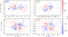 |
Fig. 5 Bivariate distribution of the rotational characteristics of vortices in the middle photosphere during the saturated phase of the SSD for the four stellar models. Every identified vortex is represented by a scatter point according to the Rortex criterion Rz and the magnetic Rortex criterion |
![Mathematical equation: $\[R_z^{\mathrm{B}}\]$](/articles/aa/full_html/2024/09/aa49401-24/aa49401-24-eq7.png)
3.2.4 Energetics
As we observe a strong correlation between swirls and twist of their magnetic field, indicating compatibility with torsional Alfvénic waves, we investigate whether these events have the potential to transport energy upward in the simulated models. To do this, we use the Poynting flux vector, defined as S = B × (v × B)/4π. Since our focus is on the vertical flux, we consider only the vertical component of the Poynting flux vector, Sz. Following Shelyag et al. (2013), Sz can be decomposed as
![Mathematical equation: $\[S_z=\underbrace{\frac{1}{4 \pi} v_z\left(B_x^2+B_y^2\right)}_{S_z^{\mathrm{v}}}-\underbrace{\frac{1}{4 \pi} B_z\left(v_x B_x+v_y B_y\right)}_{S_z^{\mathrm{h}}},\]$](/articles/aa/full_html/2024/09/aa49401-24/aa49401-24-eq15.png) (8)
(8)
where ![Mathematical equation: $\[S_z^{\mathrm{v}}\]$](/articles/aa/full_html/2024/09/aa49401-24/aa49401-24-eq16.png) is a term associated with vertical motions of the plasma, while
is a term associated with vertical motions of the plasma, while ![Mathematical equation: $\[S_z^{\mathrm{h}}\]$](/articles/aa/full_html/2024/09/aa49401-24/aa49401-24-eq17.png) is associated with horizontal motions of the plasma.
is associated with horizontal motions of the plasma.
In the following, we restrict our analysis to swirls in the middle photosphere that obey Eq. (7) and are embedded in a sufficiently strong vertical magnetic field (|Bz| > 200 G averaged over the swirl area). We refer to this selection as Alfvénic swirls. The restriction to the middle photosphere ensures that the fluxes are evaluated sufficiently far away from the top boundary, not to be strongly influenced by the reflective boundary conditions as it would be the case for the high photosphere.
Figure 7 shows the distributions of the ![Mathematical equation: $\[S_z^{\mathrm{v}}\]$](/articles/aa/full_html/2024/09/aa49401-24/aa49401-24-eq22.png) and
and ![Mathematical equation: $\[S_z^{\mathrm{h}}\]$](/articles/aa/full_html/2024/09/aa49401-24/aa49401-24-eq23.png) terms averaged over the area of the Alfvénic swirls in the middle photosphere of the four stellar models. To better visualize the distributions, a kernel density estimation (KDE) is provided. We find that for all four models, the term associated with the vertical motions of the plasma,
terms averaged over the area of the Alfvénic swirls in the middle photosphere of the four stellar models. To better visualize the distributions, a kernel density estimation (KDE) is provided. We find that for all four models, the term associated with the vertical motions of the plasma, ![Mathematical equation: $\[S_z^{\mathrm{v}}\]$](/articles/aa/full_html/2024/09/aa49401-24/aa49401-24-eq24.png) , (blue curve) peaks at negative values and has a negative skew, while the other term,
, (blue curve) peaks at negative values and has a negative skew, while the other term, ![Mathematical equation: $\[S_z^{\mathrm{h}}\]$](/articles/aa/full_html/2024/09/aa49401-24/aa49401-24-eq25.png) , (orange curve) is characterized by a positive peak and skew. This behavior is consistent with results from simulations of the solar atmosphere by Battaglia et al. (2021).
, (orange curve) is characterized by a positive peak and skew. This behavior is consistent with results from simulations of the solar atmosphere by Battaglia et al. (2021).
The sum of the two terms giving the distributions of the vertical component of the Poynting flux vector associated with Alfvénic swirls in the middle photosphere of the four models, ![Mathematical equation: $\[S_z^{\text {swirl }}\]$](/articles/aa/full_html/2024/09/aa49401-24/aa49401-24-eq26.png) , is also shown in Fig. 7 (green curve). These distributions are more centered than the other two, but retain a tendency toward positive values, both in terms of peak and skewness. As a result, the means of the four distributions have positive values, as indicated by the green vertical dashed lines in the Fig. 7 and reported in the first row of Table 3.
, is also shown in Fig. 7 (green curve). These distributions are more centered than the other two, but retain a tendency toward positive values, both in terms of peak and skewness. As a result, the means of the four distributions have positive values, as indicated by the green vertical dashed lines in the Fig. 7 and reported in the first row of Table 3.
For comparison, in the second row of Table 3 and in Fig. 7 (vertical red dashed line), we present the average vertical component of the Poynting flux vector computed over the entire domain in the middle photosphere, ![Mathematical equation: $\[S_z^{\text {tot }}\]$](/articles/aa/full_html/2024/09/aa49401-24/aa49401-24-eq27.png) . The mean vertical Poynting flux associated with Alfvénic swirls is approximately an order of magnitude larger than the mean vertical Poynting flux in the simulation box at the same height. This implies that Alfvénic swirls are associated with a substantial upward transport of energy relative to the surrounding environment. In the following, we consider the net vertical Poynting flux of Alfvénic swirls alone, disregarding possible contributions from the rest of swirls.
. The mean vertical Poynting flux associated with Alfvénic swirls is approximately an order of magnitude larger than the mean vertical Poynting flux in the simulation box at the same height. This implies that Alfvénic swirls are associated with a substantial upward transport of energy relative to the surrounding environment. In the following, we consider the net vertical Poynting flux of Alfvénic swirls alone, disregarding possible contributions from the rest of swirls.
An interesting observation is that the mean vertical Poynting flux over the computational domain increases with the effective temperature of the model, while the mean vertical Poynting flux associated with Alfvénic swirls is at a minimum in the K2V stellar model and increases again for model K8V. This result is potentially interesting in the light of studies of the ratio of the chromospheric Ca II H and K flux to the bolometric flux, log ![Mathematical equation: $\[R_{\mathrm{HK}}^{\prime}\]$](/articles/aa/full_html/2024/09/aa49401-24/aa49401-24-eq35.png) , for main-sequence stellar populations (see, e.g., Boro Saikia et al. 2018, Fig. 3). These studies show that the lower bound of chromospheric emission, known as the basal flux, is minimal and constant for stars within the range 0.5 ≤ B − V ≤ 1.1 (6000 K ≳ Teff ≳ 4500 K) and increases linearly for cooler stars down to B − V ~ 1.4 (Teff ~ 4000 K). The reason for the high basal fluxes in such cool stars remains unclear.
, for main-sequence stellar populations (see, e.g., Boro Saikia et al. 2018, Fig. 3). These studies show that the lower bound of chromospheric emission, known as the basal flux, is minimal and constant for stars within the range 0.5 ≤ B − V ≤ 1.1 (6000 K ≳ Teff ≳ 4500 K) and increases linearly for cooler stars down to B − V ~ 1.4 (Teff ~ 4000 K). The reason for the high basal fluxes in such cool stars remains unclear.
The contribution of Alfvénic swirls to the vertical Poynting flux over the total horizontal domain is,
![Mathematical equation: $\[F_{\text {swirl }}=\frac{1}{A^{\text {tot }}} \sum_{\mathrm{i}} A_i^{\text {swirl }} S_{z, i}^{\text {swirl }},\]$](/articles/aa/full_html/2024/09/aa49401-24/aa49401-24-eq36.png) (9)
(9)
where we sum over each Alfvénic swirl contribution to the vertical Poynting flux: ![Mathematical equation: $\[A_i^{\text {swirl }}=\pi\left(r_{\mathrm{eff}}^i\right)^2\]$](/articles/aa/full_html/2024/09/aa49401-24/aa49401-24-eq37.png) is the effective area of the swirl, and
is the effective area of the swirl, and ![Mathematical equation: $\[S_{z, i}^{\text {swirl }}\]$](/articles/aa/full_html/2024/09/aa49401-24/aa49401-24-eq38.png) is the vertical Poynting flux averaged over the swirl area. We also divide by the total horizontal area of the simulation domain,
is the vertical Poynting flux averaged over the swirl area. We also divide by the total horizontal area of the simulation domain, ![Mathematical equation: $\[A^{\text {tot }}=L_x^2.\]$](/articles/aa/full_html/2024/09/aa49401-24/aa49401-24-eq39.png) .
.
Additional Poynting flux may come from weak field swirls, which we have discarded here, and from swirls in regions of the magnetic network or plages, which are not included in the present SSD models. Also, the number density of swirls is about a factor three higher in the high photosphere than in the middle photosphere.
For the bolometric flux, we use Stefan-Boltzmann’s law,
![Mathematical equation: $\[F_{\mathrm{bol}}=\sigma T_{\mathrm{eff}}^4,\]$](/articles/aa/full_html/2024/09/aa49401-24/aa49401-24-eq40.png) (10)
(10)
where σ = 5.7 × 10⁻⁵ erg cm−2 s−1 K−4 is the Stefan–Boltzmann constant and Teff is the effective temperature of the star.
Assuming that a fraction r of Fswirl reaches and dissipates in the low chromosphere where the dominant radiative losses take place in the emission lines of Ca II H and K, we can compute its contribution to the chromospheric Ca II H and K flux ![Mathematical equation: $\[F_{\mathrm{HK}}^{\mathrm{swirl}}=r F_{\mathrm{swirl}}.\]$](/articles/aa/full_html/2024/09/aa49401-24/aa49401-24-eq41.png) . By taking the logarithm of the ratio between the chromospheric H and K flux due to the Alfvénic swirls and the bolometric flux, log
. By taking the logarithm of the ratio between the chromospheric H and K flux due to the Alfvénic swirls and the bolometric flux, log ![Mathematical equation: $\[R_{\mathrm{HK}}^{\prime, \text { swirl }}=\log \left(F_{\mathrm{HK}}^{\text {swirl }} / F_{\text {bol }}\right)\]$](/articles/aa/full_html/2024/09/aa49401-24/aa49401-24-eq42.png) , we get an estimate of the basal flux due to Alfvénic swirls (see Linsky et al. 1979).
, we get an estimate of the basal flux due to Alfvénic swirls (see Linsky et al. 1979).
In Table 4, we present the computed values for Fswirl, Fbol, and the basal flux proxy with r = 1 across the four stellar models. The final row includes approximate lower limits of log ![Mathematical equation: $\[R_{\mathrm{HK}}^{\prime}\]$](/articles/aa/full_html/2024/09/aa49401-24/aa49401-24-eq43.png) for stars characterized by B − V color indices of 1.37 (K8V), 0.90 (K2V), 0.65 (G2V), and 0.47 (F5V). Notably, the basal flux proxy for the K8V model surpasses those of the other stellar models. Furthermore, an approximately 70% fraction of the flux attributed to Alfvénic swirls, hence, r = 0.7, would suffice to account for the observed lower limit of basal flux in stars with B − V ~ 1.37.
for stars characterized by B − V color indices of 1.37 (K8V), 0.90 (K2V), 0.65 (G2V), and 0.47 (F5V). Notably, the basal flux proxy for the K8V model surpasses those of the other stellar models. Furthermore, an approximately 70% fraction of the flux attributed to Alfvénic swirls, hence, r = 0.7, would suffice to account for the observed lower limit of basal flux in stars with B − V ~ 1.37.
While acknowledging the hypothetical nature of this result, it introduces a novel and intriguing explanation for the significant basal fluxes observed in stars with 1.1 ≤ B − V ≤ 1.4. Concerning the remaining stellar models, the Alfvénic swirls may at least contribute to the basal flux in stars resembling the K2V and G2V types. However, such a contribution proves insufficient for the F5V model.
Mean vertical Poynting flux in the middle photosphere computed over the surface of Alfvénic swirls, ![Mathematical equation: $\[S_z^{\text {swirl }}\]$](/articles/aa/full_html/2024/09/aa49401-24/aa49401-24-eq18.png) and over the entire simulation domain,
and over the entire simulation domain, ![Mathematical equation: $\[S_z^{\text {tot }}\]$](/articles/aa/full_html/2024/09/aa49401-24/aa49401-24-eq19.png) .
.
Estimated chromospheric flux and basal flux proxy attributed to Alfvénic swirls for the four stellar models.
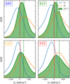 |
Fig. 7 Kernel density estimation (KDE) of the distribution of the vertical component of the Poynting flux vector associated with Alfvénic swirls, |
![Mathematical equation: $\[S_z^{\text {swirl }}\]$](/articles/aa/full_html/2024/09/aa49401-24/aa49401-24-eq30.png)
![Mathematical equation: $\[S_z^{\text {swirl }}, S_z^{\mathrm{h}}\]$](/articles/aa/full_html/2024/09/aa49401-24/aa49401-24-eq31.png)
![Mathematical equation: $\[S_z^{\mathrm{v}}\]$](/articles/aa/full_html/2024/09/aa49401-24/aa49401-24-eq32.png)
![Mathematical equation: $\[S_z^{\text {tot }}\]$](/articles/aa/full_html/2024/09/aa49401-24/aa49401-24-eq33.png)
![Mathematical equation: $\[S_z^{\text {swirl }}\]$](/articles/aa/full_html/2024/09/aa49401-24/aa49401-24-eq34.png)
3.3 Period–temperature scaling relation
In Sect. 3.2.2, we found that the rotational period of surface vortices increases with the effective temperature of stellar models. At first glance, this result may seem counterintuitive. In order to better understand this phenomenon, we construct a simplified analytical model of a stellar surface vortex. For this, we assume rotational hydrostatic equilibrium but consider the total pressure p = pgas + pmag consisting of gas and magnetic pressure instead of the gas pressure alone.
Let us consider a vertically oriented, axially symmetric vortex in rotational hydrostatic equilibrium in the surface layers of a star. We assume a constant angular velocity Ω and a uniform plasma density ρ. To describe the dynamics of this system, we use Euler’s momentum equation,
![Mathematical equation: $\[\rho \frac{D \boldsymbol{v}}{D t}=-\boldsymbol{\nabla} p+\boldsymbol{F},\]$](/articles/aa/full_html/2024/09/aa49401-24/aa49401-24-eq44.png) (11)
(11)
where Dv/Dt represents the material derivative applied to the velocity field v, p is the total pressure, and F accounts for external forces.
Equilibrium along the radial and vertical directions, ![Mathematical equation: $\[\hat{r}\]$](/articles/aa/full_html/2024/09/aa49401-24/aa49401-24-eq45.png) and
and ![Mathematical equation: $\[\hat{z}\]$](/articles/aa/full_html/2024/09/aa49401-24/aa49401-24-eq46.png) , implies that,
, implies that,
![Mathematical equation: $\[\begin{aligned}& \frac{\partial p}{\partial r}=\rho \Omega^2 r, \\& \frac{\partial p}{\partial z}=-\rho g.\end{aligned}\]$](/articles/aa/full_html/2024/09/aa49401-24/aa49401-24-eq47.png) (12)
(12)
Furthermore, due to axial symmetry, the gas pressure p depends only on the radius r and height z. Consequently, we can formulate the total derivative using the following differential expressions,
![Mathematical equation: $\[\mathrm{d} p=\frac{\partial p}{\partial r} \mathrm{~d} r+\frac{\partial p}{\partial z} \mathrm{~d} z=\rho \Omega^2 r \mathrm{~d} r-\rho g \mathrm{~d} z,\]$](/articles/aa/full_html/2024/09/aa49401-24/aa49401-24-eq48.png) (13)
(13)
where we have substituted the partial derivatives with the right-hand sides of Eq. (12). After integration, we obtain a typical pressure equation for a rotating fluid in hydrostatic equilibrium,
![Mathematical equation: $\[p-p_0=\frac{1}{2} \rho \Omega^2 r^2-\rho g\left(z-z_0\right),\]$](/articles/aa/full_html/2024/09/aa49401-24/aa49401-24-eq49.png) (14)
(14)
where p and p0 are the total pressure at coordinates (r, z) and (0, z0), respectively. In particular, Eq. (14) indicates that pressure iso-surfaces in vortex flows exhibit a parabolic shape, with the vortex core characterized by lower pressure compared to the periphery. This behavior is illustrated in Fig. 8.
If we consider a pressure isosurface (p = p0), we can derive the following scaling relation,
![Mathematical equation: $\[H_{\mathrm{p}} \sim \frac{\Omega^2 r_{\mathrm{eff}}^2}{g},\]$](/articles/aa/full_html/2024/09/aa49401-24/aa49401-24-eq50.png) (15)
(15)
where the pressure scale height, Hp, is used as the typical vertical length scale, replacing z − z0, and the radius of the vortex, reff, as the typical radius, r. Rearranging Eq. (15) and introducing the definition vϕ,eff = Ωreff, we obtain,
![Mathematical equation: $\[v_{\phi, \mathrm{eff}}^2 \sim H_{\mathrm{p}} g \sim T_{\mathrm{eff}},\]$](/articles/aa/full_html/2024/09/aa49401-24/aa49401-24-eq51.png) (16)
(16)
where we exploit the property of a stratified atmosphere where the pressure scale height Hp is proportional to Teff/g. This relationship allows the model to accurately capture the observed trend shown in the bottom panel of Fig. 4. Specifically, the model predicts that the rotational velocity of the vortices increases with the effective temperature of the star. This scaling relation is consistent with the results of Calvo et al. (2016), who found a similar relationship by considering the pressure, density, and temperature contrasts between the vortex core and the surrounding plasma.
Considering the empirical observation shown in the second panel of Fig. 4, which indicates that reff/Hp ~ const, we can refine Eq. (15) as follows,
![Mathematical equation: $\[\frac{1}{\Omega^2} \sim \frac{H_{\mathrm{p}}}{g}.\]$](/articles/aa/full_html/2024/09/aa49401-24/aa49401-24-eq52.png) (17)
(17)
Finally, using the relations Peff = 2π/Ω and Hp ~ Teff/g, we can deduce that,
![Mathematical equation: $\[P_{\mathrm{eff}} \sim \sqrt{\frac{T_{\mathrm{eff}}}{g^2}}.\]$](/articles/aa/full_html/2024/09/aa49401-24/aa49401-24-eq53.png) (18)
(18)
This equation establishes a correlation between the period of rotation of the vortex and key properties of the stellar model, namely g and Teff.
To derive a scaling relation for the rotational period that depends only on the effective temperature, we can use the Stefan-Boltzmann law and rely on empirical scaling relations established for cool, main-sequence stars (Demircan & Kahraman 1991),
![Mathematical equation: $\[\begin{aligned}& L \sim R^2 T_{\mathrm{eff}}^4, \\& L \sim M^{3.7}, \\& R \sim M^{0.9},\end{aligned}\]$](/articles/aa/full_html/2024/09/aa49401-24/aa49401-24-eq54.png) (19)
(19)
where L, M, and R represent the luminosity, mass, and radius of the star, respectively. When combined with g ~ M/R2 at the star’s surface, these relations lead to the following empirical scaling relation,
![Mathematical equation: $\[P_{\mathrm{eff}} \sim T_{\mathrm{eff}}^{2.2}.\]$](/articles/aa/full_html/2024/09/aa49401-24/aa49401-24-eq55.png) (20)
(20)
This equation confirms that the rotational period for a simplified vortex model increases with the effective temperature of the star, which supports the statistical results obtained from the simulations.
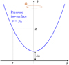 |
Fig. 8 Two-dimensional representation of an axially symmetric flow rotating at angular velocity Ω. The surface of constant pressure p = p0 is shown, where p0 is the pressure at (r, z) = (0, z0). |
4 Summary and conclusions
In this paper, we carried out an analysis on three-dimensional, radiative-MHD, numerical simulations of the atmospheres of main sequence dwarfs of the spectral types K8V, K2V, G2V, and F5V. The focus was on the properties of vortex motions within different layers of the simulation domain. In particular, we investigated how these properties are affected by the strength of the magnetic field, which is amplified by the action of a subsurface SSD.
As expected, vortex motions are found to be ubiquitous in numerical simulations of stellar atmospheres also other than the solar one. However, we found that different properties of the vortices depend on the characteristics of the stellar model and on the strength of the surface magnetic field. The presence of a strong magnetic field led to a reduction in the number and rotational speed of vortices in the surface layers of the convection zone, due to magnetic quenching. However, sufficiently high in the photosphere, an increased number of vortices showing higher rotational velocities were found in all four stellar models with respect to the weak field (kinematic) phase, highlighting the fundamental role of the magnetic field in the formation and dynamics of small-scale swirls in stellar atmospheres.
The size of the vortices was observed to be larger in hotter stars. However, when normalized to the average pressure scale height at the surface, the average radius of the swirls became nearly constant across the different stellar models and layers, being about one fourth of the pressure scale height. This result suggests a direct correlation between the size of the vortices and the scale of the flows, particularly the granular and intergranular flows. However, to firmly establish this correlation, a resolution study is still needed to assess how this result is being affected by the numerical spatial resolution of the simulations (see, e.g., Yadav et al. 2020).
We investigate the relation between stellar swirls and perturbations in the surface magnetic fields generated by saturated SSD action. Our investigation reveals a robust correlation between swirls and twists in the magnetic field, suggesting that over 80% of the swirls in the middle photosphere are consistent with torsional Alfvénic waves. These events, especially when associated with a sufficiently strong vertical magnetic field, contribute to an average, upward energy flux that exceeds by an order of magnitude the average Poynting flux over the entire simulation box. This result highlights that swirls associated with Alfvénic pulses, termed Alfvénic swirls, have the potential to play a significant role in the transport of energy to the upper layers of stellar atmospheres.
Moreover, our investigation reveals that the average vertical Poynting flux associated with Alfvénic swirls is higher in the K8V model compared to the K2V model. This observation holds particular significance in the context of studies on chromospheric activity in main sequence stars. Specifically, if approximately 70% of the vertical Poynting flux linked to Alfvénic swirls in the middle photosphere of the K8V model reaches the low chromosphere and dissipates, it could potentially explain the heightened basal flux observed on stars with B − V ~ 1.4. This hypothesis introduces a novel framework for interpreting the heightened basal fluxes observed in stars within the range 1.1 ≤ B − V ≤ 1.4, offering valuable insights into understanding chromospheric activity in cool stars.
Furthermore, we discovered that the rotational period of swirls increases with the effective temperature of the stellar model. This finding is not trivial, considering that hotter stars typically exhibit faster swirl rotations due to higher flow velocities. Based on a simple model of a vortex in rotational hydrostatic equilibrium and incorporating empirical mass-luminosity and mass-radius scaling relations for cool, main-sequence stars, we derived a scaling relation connecting the rotational period with the effective temperature of the stellar model, ![Mathematical equation: $\[P_{\mathrm{eff}} \propto T_{\mathrm{eff}}^{2.2}\]$](/articles/aa/full_html/2024/09/aa49401-24/aa49401-24-eq56.png) . This relation supports the results obtained from the statistical analysis.
. This relation supports the results obtained from the statistical analysis.
In conclusion, our study demonstrates the existence of swirls in numerical models of stellar atmospheres, with their specific properties depending on the properties of the stellar models. In addition, we propose that torsional Alfvénic pulses associated with small-scale swirling motions may be an important contributor to the basal flux in Ca II H and K (S-index) of cool stars, in particular with respect to the enhanced basal flux in the range 1.1 ≤ B − V ≤ 1.4. Although this hypothesis involves some crude assumptions, it effectively reproduces the trend of the observed fluxes and is therefore worth considering.
To make further progress, simulations of a wider parameter space, a finer model grid, and additional magnetic field configurations are needed for a more detailed comparison with measurements of the S-index. Also for these simulations, the chromospheric layers and corresponding physics should be taken into account, which would make it possible to compute the CaII H and K fluxes directly from the models and to compute a synthetic S-index and ![Mathematical equation: $\[R_{\mathrm{HK}}^{\prime}\]$](/articles/aa/full_html/2024/09/aa49401-24/aa49401-24-eq57.png) conversion.
conversion.
The upper boundary of the computational domain must then be set sufficiently far above the spectral line forming layers and must be made transparent to torsional Alfvén waves. Including and excluding the areas of Alfvénic swirls would then provide more insights into the role of these kind of swirls for the chromospheric basal flux of cool stars. By continuing to study these phenomena, we can gain a more complete understanding of the intricate processes that take place in stellar atmospheres and their impact on stellar systems.
Acknowledgements
The authors acknowledge support by the Swiss National Science Foundation under grant ID 200020_182094 and the University of Zürich under grant UZH Candoc 2022 ID 7104. This work has profited from discussions with the team of K. Tziotiou and E. Scullion (conveners) “The Nature and Physics of Vortex Flows in Solar Plasma” and with the team of P. Keys (convener) “WaLSA: Waves in the Lower Solar Atmosphere at High Resolution” (www.walsa.team), both at the International Space Science Institute (ISSI). Part of the numerical simulations were carried out on Piz Daint at CSCS under project IDs s1059, s1172, and u14, and the rest was carried out on the HPC ICS cluster at USI.
Appendix A Surface distribution of swirls in the kinematic phase and nonmagnetic bright points
Figure A.1 shows the density ρ at the average τR = 1 surface for the K8V, K2V, G2V, and F5V models at the same time instances as in Fig. 1. The figure shows a granulation pattern consistent with that of Fig. 1, characterized by cells of bright and warm upflowing plasma surrounded by denser, cooler intergranular downdrafts. Figure A.2 zooms in on two regions of the K8V and F5V models, accompanied by instantaneous streamlines of the horizontal velocity field. Similar to Figs. 1 and 2, the vortices identified by the SWIRL algorithm are represented by disks which size and color is defined by their effective radius and direction of rotation, respectively.
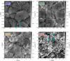 |
Fig. A.1 Density ρ at the average τR = 1 surface for the K8V, K2V, G2V, and F5V models during the kinematic phase. Pink and green disks correspond to the clockwise and counter-clockwise vortices identified by the SWIRL algorithm. The blue squares in the K8V and F5V panels represent the boundaries of the zoom-in plots shown in Fig. A.2. |
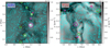 |
Fig. A.2 Identified swirls in the areas depicted in blue in Fig. A.1 for the K8V and F5V models. Pink disks represent clockwise swirls, green counter-clockwise swirls. The horizontal component of the velocity field is represented by blue instantaneous streamlines. |
These figures confirm the visual impression conveyed by Fig. 1, indicating that the majority of vortices are located within or in close proximity to intergranular flows. It is also apparent that certain bright features that can be found in the maps of bolometric intensity, commonly referred to as nonmagnetic bright points, are associated with low density regions and swirling motions. A prominent example is shown in the left panel of Figs. 2 and A.2 at (x, y) = (1.10, 0.25) Mm. These events, previously observed in numerical simulations of the solar atmosphere by Calvo et al. (2016), are here identified in simulations of other stellar types as well.
Appendix B Distribution of swirls in the saturation phase and magnetic bright points
This appendix illustrates the distribution of swirls in the K8V model at the surface and in the high photosphere during the saturation phase of the small-scale dynamo (SSD). Figure B.1 shows the emerging bolometric intensity, Ibol, and the swirls identified by the SWIRL algorithm at z = 0 km. The qualitative properties of swirls during this phase appear similar to those shown in Figs. 1 and 2 for the kinematic phase.
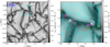 |
Fig. B.1 Emerging bolometric intensity, Ibol, for the K8V stellar model during the saturation phase of the SSD. Clockwise and counterclockwise vortices in the horizontal plane at z = 0 km identified by the SWIRL algorithm are indicated by pink and green disks, respectively. The blue square in the left panel marks the boundaries of the zoomed region shown in the right panel, where the horizontal component of the velocity field at z = 0 km is represented by blue instantaneous streamlines. |
However, we note that a key difference between the kinematic and saturation phases is the nature of the bright features observed in the bolometric intensity. As a matter of fact, the bright features in Fig. B.1 (that is, in the saturation phase), known as magnetic bright points, indicate the presence of intense magnetic flux tubes that are rooted in intergranular vertices and extend vertically throughout the atmosphere. The presence of these vertically extending magnetic flux concentrations is highlighted in Fig. B.2, which shows the vertical magnetic field, Bz, in the high photosphere for the same K8V model and time instance as of Fig. B.1.
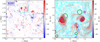 |
Fig. B.2 Vertical magnetic field, Bz, for the K8V stellar model during the saturation phase of the SSD in the high photosphere (z = 183 km). Clockwise and counterclockwise vortices identified by the SWIRL algorithm in the horizontal plane are indicated by pink and green disks, respectively. The blue square in the left panel marks the boundaries of the zoomed region shown in the right panel, where the horizontal component of the velocity field at z = 183 km is represented by blue instantaneous streamlines. |
The comparison of Figs. B.1 with B.2 shows that there are swirls on the stellar surface, associated with magnetic bright points, which extend vertically and reach the upper layers of the stellar atmosphere. Indeed, the right panels of these two figures show on the surface two clockwise-rotating swirls, associated with two magnetic bright points, located at (x, y) = (0.92, 1.78) Mm and (x, y) = (1.18, 1.72) Mm, respectively, that are found at approximately the same coordinates in the high photosphere and embedded in positive polarity magnetic field. Similar coherent vortical structures have been studied in detail by Canivete Cuissa & Steiner (2024) for numerical simulations of the solar atmosphere with a non-SSD generated magnetic field, showing that more than 80% of them may be of Alfvénic nature.
The instantaneous streamlines of the horizontal velocity field shown in the right panels of Figs. B.1 and B.2 demonstrate the effectiveness of the SWIRL code in detecting vortical motions in the different horizontal planes of the simulated models also in the presence of magnetic fields. This underscores the robustness of the SWIRL algorithm in identifying vortices under varying conditions within the stellar atmosphere.
References
- Battaglia, A. F., Canivete Cuissa, J. R., Calvo, F., Bossart, A. A., & Steiner, O. 2021, A&A, 649, A121 [NASA ADS] [CrossRef] [EDP Sciences] [Google Scholar]
- Beeck, B., Schüssler, M., & Reiners, A. 2011, arXiv e-prints [arXiv:1101.3848] [Google Scholar]
- Bonet, J. A., Márquez, I., Sánchez Almeida, J., Cabello, I., & Domingo, V. 2008, ApJ, 687, L131 [Google Scholar]
- Boro Saikia, S., Marvin, C. J., Jeffers, S. V., et al. 2018, A&A, 616, A108 [NASA ADS] [CrossRef] [EDP Sciences] [Google Scholar]
- Brandenburg, A., & Subramanian, K. 2005, Phys. Rep., 417, 1 [NASA ADS] [CrossRef] [Google Scholar]
- Calvo, F., Steiner, O., & Freytag, B. 2016, A&A, 596, A43 [NASA ADS] [CrossRef] [EDP Sciences] [Google Scholar]
- Canivete Cuissa, J. R. 2022, https://zenodo.org/doi/10.5281/zenodo.10016646 [Google Scholar]
- Canivete Cuissa, J. R., & Steiner, O. 2020, A&A, 639, A118 [EDP Sciences] [Google Scholar]
- Canivete Cuissa, J. R., & Steiner, O. 2022, A&A, 668, A118 [NASA ADS] [CrossRef] [EDP Sciences] [Google Scholar]
- Canivete Cuissa, J. R., & Steiner, O. 2024, A&A, 682, A181 [NASA ADS] [CrossRef] [EDP Sciences] [Google Scholar]
- Demircan, O., & Kahraman, G. 1991, Ap&SS, 181, 313 [Google Scholar]
- Freytag, B., Steffen, M., Ludwig, H. G., et al. 2012, J. Computat. Phys., 231, 919 [NASA ADS] [CrossRef] [Google Scholar]
- Linsky, J. L., Worden, S. P., McClintock, W., & Robertson, R. M. 1979, ApJS, 41, 47 [NASA ADS] [CrossRef] [Google Scholar]
- Liu, J., Nelson, C. J., Snow, B., Wang, Y., & Erdélyi, R. 2019, Nat. Commun., 10, 3504 [Google Scholar]
- Lugt, H. J. 1979, The Dilemma of Defining a Vortex, eds. U. Müller, K. G. Roesner, & B. Schmidt (Berlin, Heidelberg: Springer Berlin Heidelberg), 309 [Google Scholar]
- Magic, Z., Collet, R., Asplund, M., et al. 2013, A&A, 557, A26 [NASA ADS] [CrossRef] [EDP Sciences] [Google Scholar]
- Moll, R., Cameron, R. H., & Schüssler, M. 2011, A&A, 533, A126 [NASA ADS] [CrossRef] [EDP Sciences] [Google Scholar]
- Moll, R., Cameron, R. H., & Schüssler, M. 2012, A&A, 541, A68 [NASA ADS] [CrossRef] [EDP Sciences] [Google Scholar]
- Nordlund, A. 1985, Sol. Phys., 100, 209 [NASA ADS] [CrossRef] [Google Scholar]
- Priest, E. 2014, Magnetohydrodynamics of the Sun (Cambridge University Press), https://doi.org/10.1017/CBO9781139020732 [Google Scholar]
- Riva, F., Steiner, O., & Freytag, B. 2024, A&A, 684, A7 [NASA ADS] [CrossRef] [EDP Sciences] [Google Scholar]
- Rodriguez, A., & Laio, A. 2014, Science, 344, 1492 [NASA ADS] [CrossRef] [Google Scholar]
- Sadarjoen, I. A., & Post, F. H. 1999, in Data Visualization ’99, eds. E. Gröller, H. Löffelmann, & W. Ribarsky (Vienna: Springer Vienna), 53 [Google Scholar]
- Salhab, R. G., Steiner, O., Berdyugina, S. V., et al. 2018, A&A, 614, A78 [NASA ADS] [CrossRef] [EDP Sciences] [Google Scholar]
- Shelyag, S., Cally, P. S., Reid, A., & Mathioudakis, M. 2013, ApJ, 776, L4 [Google Scholar]
- Tian, S., Gao, Y., Dong, X., & Liu, C. 2018, J. Fluid Mech., 849, 312 [NASA ADS] [CrossRef] [Google Scholar]
- Tziotziou, K., Scullion, E., Shelyag, S., et al. 2023, Space Sci. Rev., 219, 1 [NASA ADS] [CrossRef] [Google Scholar]
- Wang, Y.-q., Gao, Y.-s., Liu, J.-m., & Liu, C. 2019, J. Hydrodyn., 31, 464 [NASA ADS] [CrossRef] [Google Scholar]
- Wedemeyer, S., & Steiner, O. 2014, PASJ, 66, S10 [Google Scholar]
- Wedemeyer, S., Ludwig, H. G., & Steiner, O. 2013, Astron. Nachr., 334, 137 [NASA ADS] [CrossRef] [Google Scholar]
- Wedemeyer-Böhm, S., Scullion, E., Steiner, O., et al. 2012, Nature, 486, 505 [Google Scholar]
- Witzke, V., Duehnen, H. B., Shapiro, A. I., et al. 2023, A&A, 669, A157 [NASA ADS] [CrossRef] [EDP Sciences] [Google Scholar]
- Yadav, N., Cameron, R. H., & Solanki, S. K. 2020, ApJ, 894, L17 [Google Scholar]
- Zhou, J., Adrian, R. J., Balachandar, S., & Kendall, T. M. 1999, J. Fluid Mech., 387, 353 [Google Scholar]
The term Alfvénic (instead of Alfvén) is used to remind readers that these pulses or waves are not purely but mainly of an Alfvénic nature. They may also exhibit a compressive component.
For the four simulations, the maximum values of ⟨Ekin/Emag⟩conv are around 0.10. For further details, the reader can refer to Riva et al. (2024).
Vortices detected inside a granule are generally located in a region where an intergranular lane is forming. Therefore, their origin might be associated to the formation of a new granule.
All Tables
Mean vertical Poynting flux in the middle photosphere computed over the surface of Alfvénic swirls, and over the entire simulation domain, .
Estimated chromospheric flux and basal flux proxy attributed to Alfvénic swirls for the four stellar models.
All Figures
|
Fig. 1 Emerging bolometric intensity, Ibol, for the K8V, K2V, G2V, and F5V models during the kinematic phase. Clockwise and counterclockwise vortices in the horizontal plane at z = 0 identified by the SWIRL algorithm are indicated by pink and green disks, respectively. The blue squares in the K8V and F5V panels mark the boundaries of the zoomed plots shown in Fig. 2. |
| In the text | |
|
Fig. 2 Identified swirls in the areas marked in blue in Fig. 1 for the K8V and F5V models. Clockwise and counterclockwise vortices identified by the SWIRL algorithm are indicated by pink and green disks, respectively. The horizontal component of the velocity field is represented by blue instantaneous streamlines. |
| In the text | |
|
Fig. 3 Bivariate distribution of the bolometric intensity Ibol and the absolute vertical magnetic field |Bz| in the center of the swirls identified on the surface layer at z = 0 km of the four stellar models. The distributions during the kinematic and saturation phases are shown in blue and orange, respectively. The vertical black dotted lines indicate the mean bolometric intensity in the intergranular (lower value) and granular (higher value) regions. The red shaded area indicates the identification range of magnetic bright feature (MBF) as defined by Riva et al. (2024). |
| In the text | |
|
Fig. 4 Properties of the swirls during the kinematic and saturation phases of the SSD and at different heights in the atmosphere of the four stellar models. The average number of swirls per granule in the simulation domain (top), the average ratio between radius and pressure scale height, reff/Hp (middle-top), rotational period, Peff (middle-bottom), and plasma rotational velocity vϕ,eff (bottom), are shown. The heights of the cross sections labeled as convection zone, surface, middle photosphere, and higher photosphere are given in Table 2 for the four stellar models. |
| In the text | |
|
Fig. 5 Bivariate distribution of the rotational characteristics of vortices in the middle photosphere during the saturated phase of the SSD for the four stellar models. Every identified vortex is represented by a scatter point according to the Rortex criterion Rz and the magnetic Rortex criterion |
| In the text | |
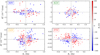 |
Fig. 6 Same as Fig. 5 but for the high photosphere. |
| In the text | |
|
Fig. 7 Kernel density estimation (KDE) of the distribution of the vertical component of the Poynting flux vector associated with Alfvénic swirls, |
| In the text | |
|
Fig. 8 Two-dimensional representation of an axially symmetric flow rotating at angular velocity Ω. The surface of constant pressure p = p0 is shown, where p0 is the pressure at (r, z) = (0, z0). |
| In the text | |
|
Fig. A.1 Density ρ at the average τR = 1 surface for the K8V, K2V, G2V, and F5V models during the kinematic phase. Pink and green disks correspond to the clockwise and counter-clockwise vortices identified by the SWIRL algorithm. The blue squares in the K8V and F5V panels represent the boundaries of the zoom-in plots shown in Fig. A.2. |
| In the text | |
|
Fig. A.2 Identified swirls in the areas depicted in blue in Fig. A.1 for the K8V and F5V models. Pink disks represent clockwise swirls, green counter-clockwise swirls. The horizontal component of the velocity field is represented by blue instantaneous streamlines. |
| In the text | |
|
Fig. B.1 Emerging bolometric intensity, Ibol, for the K8V stellar model during the saturation phase of the SSD. Clockwise and counterclockwise vortices in the horizontal plane at z = 0 km identified by the SWIRL algorithm are indicated by pink and green disks, respectively. The blue square in the left panel marks the boundaries of the zoomed region shown in the right panel, where the horizontal component of the velocity field at z = 0 km is represented by blue instantaneous streamlines. |
| In the text | |
|
Fig. B.2 Vertical magnetic field, Bz, for the K8V stellar model during the saturation phase of the SSD in the high photosphere (z = 183 km). Clockwise and counterclockwise vortices identified by the SWIRL algorithm in the horizontal plane are indicated by pink and green disks, respectively. The blue square in the left panel marks the boundaries of the zoomed region shown in the right panel, where the horizontal component of the velocity field at z = 183 km is represented by blue instantaneous streamlines. |
| In the text | |
Current usage metrics show cumulative count of Article Views (full-text article views including HTML views, PDF and ePub downloads, according to the available data) and Abstracts Views on Vision4Press platform.
Data correspond to usage on the plateform after 2015. The current usage metrics is available 48-96 hours after online publication and is updated daily on week days.
Initial download of the metrics may take a while.