© The Authors 2023

1 Introduction

Protoplanetary disks, the rotationally-supported excess from the star-formation process, consist primarily of hydrogen and helium gas, with trace molecular species. Despite its preponderance by mass, this gas component has a low frequency-integrated opacity, making direct radiative heating and cooling inefficient. The disk’s energy exchange with the radiation field is instead mediated by the dust component, typically taken to constitute just 1% of its total mass. Chiang & Goldreich (1997) studied this process semi-analytically, finding that incident stellar radiation – which peaks in the visible and near-infrared for classical T Tauri stars – creates a superheated dust layer at a disk’s radial τ_r = 1 surface. This layer reprocesses the radiation into the thermal infrared, half of which dissipates into interstellar space and half of which radiatively diffuses through dust grains in the optically thick disk midplane. The surrounding gas is then thermally coupled to the dust temperature structure via collisions. In turn, the density structure of the gas and, consequently, that of the entrained dust that sets the τ_r = 1 surface, adapts to maintain hydrostatic equilibrium.

By far, the most detailed models of protoplanetary disk thermal structure come from physical-chemical codes (e.g., Woitke et al. 2009; Bruderer et al. 2012; Bruderer 2013; Calahan et al. 2021), followed by standalone, multiwavelength radiative transfer codes (e.g., Dullemond et al. 2012; Whitney et al. 2013). However, the computational expense of these numerical algorithms, along with their implicit assumption that disks are static on timescales relevant to thermal physics, makes them intractable to include in dynamical problems. Hydrodynamical simulations must therefore use various parametrizations, of which the “locally isothermal” assumption, whereby the temperature in each grid cell is fixed to its initial value, has been historically important for its simplicity and ease of interpretation. However, more recently, simulations of hydrodynamic instabilities and the anticyclonic vortices they generate (Malygin et al. 2017; Pierens & Lin 2018; Tarczay-Nehéz et al. 2020; Manger et al. 2021; Huang & Yu 2022), gaps and rings (Miranda & Rafikov 2019; Ziampras et al. 2020), spiral arms (Miranda & Rafikov 2020a,b), and circumplanetary disks (Fung et al. 2019) have revealed that the choice of disk thermodynamics prescription has a substantial influence on their morphology and behavior. The quality of disk observations continues to improve (e.g. Keppler et al. 2018; Ren et al. 2018; Teague et al. 2019; Pinte et al. 2022) and meaningfully interpreting them requires a more accurate, self-consistent treatment of disk heating and cooling in hydrodynamic models.

To this end, numerical radiation hydrodynamics (RHD) is promising. For computational efficiency, these simulations generally use the “grey approximation” in which radiation energy densities, fluxes, and material opacities are averaged over frequency. One widely used method in the study of protoplanetary disks (e.g., Klahr & Kley 2006; Kley et al. 2009; Bitsch et al. 2013; Flock et al. 2013; Binkert et al. 2023) is flux-limited diffusion (FLD; Levermore & Pomraning 1981), in which the radiative flux, F_r, is proportional to the gradient of radiation energy density E_r, subject to a limiter that ensures the system satisfies the speed-of-light limit, |F_r| ≤ cE_r. Although FLD works well in optically thick regions, its definition of flux is limited in the thin limit, making it unable to produce anisotropic features in the radiation field such as beams or shadows. The M1 approximation (Levermore 1984) handles these issues with a separate evolution equation for flux. M1 can accurately reproduce both the optically thick diffusion and optically thin free-streaming limits, but has limitations in situations where free-streaming beams cross one another.

Differentiating between dust and gas temperatures is a comparatively recent development in RHD simulations. The star-formation simulations of Bate & Keto (2015), as well as the thermochemical disk simulations of Wang & Goodman (2017), Wang et al. (2019) and Hu et al. (2023), use equilibrium prescriptions to compute dust temperature. By contrast, Pavlyuchenkov & Zhilkin (2013), Pavlyuchenkov et al. (2015), and Vorobyov et al. (2020) use iterative Newton-Raphson schemes to self-consistently compute energy exchange between gas, dust, and radiation, while using FLD for radiation transport.

In what follows, we present our own three-temperature scheme, implemented within the PLUTO hydrodynamics code (Mignone et al. 2007). To compute the energy exchange, we use Newton-Raphson iterations (albeit with differences from the aforementioned works) and to transport radiation, we use the M1 scheme already developed for PLUTO (Melon Fuksman & Mignone 2019; Melon Fuksman et al. 2021) to handle both the optically thick and thin regimes in protoplanetary disks. Section 2 describes our numerical method. Section 3 details our code tests: the first two (0D matter-radiation coupling and 1D Ensman shock tube) have known reference solutions and demonstrate basic function, while the latter two (2D self-shadowing and 3D disk-planet interaction) illustrate applications to realistic disks. Section 4 provides a summation of our work and discusses possible future areas of research.

2 Method

2.1 Basic equations

We developed a strategy to solve the equations of radiation hydrodynamics, including a secondary dust fluid. We made the simplifying assumptions that dust grains are kinetically well-coupled to the gas (Stokes number St ≪ 1) and that they have negligible inertia (globally constant dust-to-gas ratio of f_d ≪ 1), in other words, both evolve with the same velocity field and the dust has no momentum: $$\frac{\partial \rho }{\partial t}+\nabla \cdot \left(\rho \upsilon \right)=0,$$(1a) $$\frac{\partial \left(\rho \upsilon \right)}{\partial t}+\nabla \cdot \left(\rho \upsilon \upsilon \right)=-{\nabla }_p-\rho \nabla \text{Φ\hspace{0.17em}}+S_m+G,$$(1b) $$\frac{\partial E_{\text{g}}}{\partial t}+\nabla \cdot \left(E_{\text{g}}\upsilon \right)=-\nabla \cdot \left(\left(p+\rho \text{Φ}\right)\upsilon \right)+S_m+X_{gd}+c{G}_{\text{g}}+S_{\text{g}}^{\text{irr}},$$(1c) $$\frac{\partial E_{\text{d}}}{\partial t}+\nabla \cdot \left(E_{\text{d}}\upsilon \right)=-X_{gd}+c{G}_d+S_{\text{d}}^{\text{irr}},$$(1d) $$\frac{\partial E_r}{\partial t}+\widehat{c}\nabla \cdot F_r=-\widehat{c}\left(G_{\text{g}}+G_d\right),$$(1e) $$\frac{\partial F_r}{\partial t}+\widehat{c}\nabla \cdot P_r=-\widehat{c}G,$$(1f)

where p, υ, p represent the gas density, pressure, and velocity respectively. Also, ρ_d is the dust density, while f_d is the dust-to-gas ratio, Φ is the gravitational potential, and {E_g, E_d, E_r} are the total energy densities for gas, dust, and radiation respectively. Then, c is the speed of light, while the ĉ term is a “reduced speed of light” (Gnedin & Abel 2001) which enables longer timesteps, but must nevertheless exceed all hydrodynamic velocities relevant to the problem (Skinner & Ostriker 2013).

We assume that the gas follows an ideal equation of state: $$p={\rho }_{\text{g}}{k}_{\text{B}}{T}_{\text{g}}/\mu m_{\text{H}},$$(2)

where k_B is the Boltzmann constant, T_g the gas temperature, µ the mean molecular weight, and m_H the mass of a hydrogen atom. The adiabatic index γ = ∂ In p/∂ In ρ is a constant, implying an internal (thermal) energy density: $${\xi }_{\text{g}}=p/\left(\gamma -1\right).$$(3)

Because we do not consider the kinetic energy of dust in this work, the internal energy of dust, ξ_d, is equal to its total energy E_d. For consistency of notation in what follows, we additionally define a symbol ξ_r = E_r.

Dust and gas exchange internal energy collisionally via the term $$X_{gd}\equiv t_{\text{c}}^{-1}\left(r_{\text{gd}}{\xi }_{\text{d}}-{\xi }_{\text{g}}\right),$$(4)

where t_c is the thermal relaxation time and r_gd = k_B/µm_Hf_dc_d(γ − 1) is the ratio of heat capacity per unit volume between gas and dust. Also, c_d is the specific heat capacity of dust. We compute the gas cooling time, t_c, as a function of the dust-gas stopping time, t_s, in the Epstein regime (Burke & Hollenbach 1983; Speedie et al. 2022): $$t_{\text{c}}=\frac{2/3}{\gamma -1}{f}_{\text{d}}^{-1}{t}_{\text{s}}{\eta }^{-1},$$(5)

where η is an order-unity “accommodation coefficient,” which we ignore going forward. The corresponding dust cooling time is given by: $$t_{c,\text{dust}}=r_{\text{gd}}^{-1}{t}_c=\frac{2}{3}\frac{c_{\text{d}}}{k_{\text{B}}/\mu m_{\text{H}}}{t}_{\text{s}}.$$(6)

In a realistic disk, the stopping time is computed by averaging over a grain-size distribution, which we describe as part of Sect. 3.3. The usual two-temperature radiation hydrodynamics represents the limit where t_c → 0.

Net radiative heating and cooling is given for the gas by $$\begin{array}{l}{G}_{\text{g}}\equiv -\rho {\kappa }_g\left(a_{\text{r}}{T}_{\text{g}}^4-{\xi }_{\text{r}}\right)\hfill \\ -\rho \left(2{\kappa }_g-{\chi }_g\right)\beta \cdot F_r-\rho {\chi }_g\beta \cdot \left({\xi }_{\text{r}}\beta +\beta \cdot P_r\right),\hfill \end{array}$$(7a)

and likewise for dust by $$\begin{array}{l}{G}_d\equiv -\rho {\kappa }_d{f}_{\text{d}}\left(a_{\text{r}}{T}_{\text{d}}^4-{\xi }_{\text{r}}\right)\hfill \\ -\rho f_{\text{d}}\left(2{\kappa }_d-{\chi }_{\text{d}}\right)\beta \cdot F_r-\rho f_{\text{d}}{\chi }_d\beta \cdot \left({\xi }_{\text{r}}\beta +\beta \cdot P_r\right).\hfill \end{array}$$(7b)

Similarly, the attenuation of radiative flux by gas is given by $$\begin{array}{l}{G}_{\text{g}}\equiv \rho {\chi }_{\text{g}}{F}_r-\rho {\kappa }_g\left(a_{\text{r}}{T}_{\text{g}}^4-{\xi }_{\text{r}}\right)\beta \hfill \\ -2\rho {\kappa }_g\left(\beta \cdot F_r\right)\beta -\rho {\chi }_g\left({\xi }_{\text{r}}\beta +\beta \cdot P_r\right),\hfill \end{array}$$(7c)

and for dust by $$\begin{array}{l}{G}_d\equiv \rho f_{\text{d}}{\chi }_{\text{d}}{F}_r-\rho f_{\text{d}}{\kappa }_d\left(a_{\text{r}}{T}_{\text{d}}^4-{\xi }_{\text{r}}\right)\beta \hfill \\ -2\rho f_{\text{d}}{\kappa }_d\left(\beta \cdot F_r\right)\beta -\rho f_{\text{d}}{\chi }_d\left({\xi }_{\text{r}}\beta +\beta \cdot P_r\right),\hfill \end{array}$$(7d)

involving absorption opacities κ, total (absorption plus scattering) opacities χ, temperatures T, the radiation constant, a_r = 4σ_SB/c, and the radiation pressure tensor P_r. Typically, κ is computed as a Planck average over frequency, while χ is computed as a Rosseland average. We define G = G_G + G_d; because our current implementation assumes dust follows the gas and has negligible inertia, it is this total G that gets added to the gas momentum equation and integrated during the hydrodynamic step.

Each of the expressions in Eq. (7) can be divided into a β-independent and β-dependent part, G = G^w + G′ (β). The G′ (β) parts arise from a Lorentz transformation of the radiation-interaction terms from the fluid’s comoving frame to the observer’s frame, truncated in the mildly relativistic regime (Skinner & Ostriker 2013; Melon Fuksman & Mignone 2019). In protoplanetary disks, β ≪ 1¹, so these terms are small and can be integrated explicitly.

The radiation pressure tensor P_r(E_r, F_r) is evaluated according to the Ml closure (Levermore 1984), which accurately reproduces the free-streaming and diffusion limits: $$P_r^{ij}=D^{ij}{E}_r=E_r\left(\frac{1-\text{Ξ}}{2}{\delta }^{ij}+\frac{3\text{Ξ}-1}{2}{n}^i{n}^i\right),$$(8)

in which $$\text{Ξ=}\frac{3+4w^2}{5+2\sqrt{4-3w^2}},$$(9)

where n = F_r/||F_r||, w = ||F_r||/E_r, and δ^ij is the Kronecker delta.

Here, $S_{\text{d}}^{\text{irr}}$ and $S_{\text{g}}^{\text{irr}}$ represent radiation emitted directly by the star, which has a higher frequency spectrum than the dust-emitted radiation represented by E_r; the source terms are computed (e.g., via ray tracing) at every hydrodynamic timestep, rather than being evolved dynamically as E_r and F_r are. Then, S_m and S_m represent the energy and momentum source terms, respectively, such as the thermal conductivity and viscosity that are already implemented into PLUTO and integrated during the hydrodynamic step.

2.2 Conservation laws

With the reduced speed of light approximation, and ignoring non-ideal source terms other than G_g, G_d, G_g, G_d, X_gd, our system conserves the following modified total energy and momentum: $$E_{\text{tot}}=E_r\left(c/\widehat{c}\right)+E_{\text{g}}+E_{\text{d}}={\xi }_{\text{r}}\left(c/\widehat{c}\right)+{\xi }_{\text{g}}+{\xi }_{\text{d}}+\rho {\upsilon }^2/2,$$(10) $$P_{\text{tot}}=F_r/\widehat{c}+p_{\text{g}}$$(11)

which are reduced to the standard definitions when c = ĉ. As mentioned earlier, Skinner & Ostriker (2013) verified that this modification does not impact the dynamics of the system, provided that ĉ is much larger than hydrodynamic velocities characteristic of the system.

2.3 Operator splitting and timestepping

We solve the dusty radiation-hydrodynamic (Eq. (1)) using a Strang split, sandwiching a full step of the hydrodynamic terms Δt between two half-steps Δt/2 of the radiative terms. In quasi-conservative form: $$\frac{\partial \text{𝒰}}{\partial t}+\left(\nabla ·{ℱ}_{\text{HD}}+\nabla ·{ℱ}_{\text{rad}}\right)=\left(S_{\text{HD}}+S_{\text{rad}}^{\text{imp}}+S_{\text{rad}}^{\exp }\right),$$(12a)

where 𝒰 is a vector of conserved variables, 𝒮 are source terms, and ℱ are advective fluxes: $$𝒰={\left(\rho ,\rho \upsilon ,E_{\text{g}},E_{\text{d}},E_r,F_r\right)}^{\top },$$(12b) $${\text{ℱ}}_{\text{HD}}={\left(\rho \upsilon ,\rho \upsilon \upsilon +pI,\left(E_{\text{g}}+p+\rho \text{Φ}\right)\upsilon ,E_{\text{d}}\upsilon ,0,0\right)}^{\top },$$(12c) $${\text{ℱ}}_{\text{rad}}={\left(0,0,0,0,\widehat{c}{E}_r,\widehat{c}{P}_r\right)}^{\top },$$(12d) $${\text{𝒮}}_{\text{HD}}={\left(0,-\rho \nabla \text{Φ}+S_m,S_m,0,0,0\right)}^{\top },$$(12e) $$\begin{array}{l}{\text{𝒮}}_{\text{rad}}^{\text{imp}}=(0,G^{\text{w}},X_{gd}+c{G}_{\text{g}}^{\text{w}}+S_{\text{g}}^{\text{irr}}\hfill \\ {-X_{gd}+c{G}_d+S_{\text{d}}^{\text{irr}},-\widehat{c}\left(G_{\text{g}}+G_d\right),-\widehat{c}G)}^{\top },\hfill \end{array}$$(12f) $${\text{𝒮}}_{\text{rad}}^{\exp }={\left(0,G^{\prime },c{G^{\prime }}_{\text{g}},c{G^{\prime }}_d,-\widehat{c}\left({G^{\prime }}_{\text{g}}+{G^{\prime }}_d\right),-\widehat{c}{G}^{\prime }\right)}^{\top }.$$(12g)

The overall timestep duration Δt is set by applying the Courant criterion to the hydrodynamical signal speeds υ_HD. But because ĉ ≫ υ_HD, the radiation half-steps Δt/2 must be further divided into substeps of duration Δt_rad to ensure that the radiation subsystem meets its own Courant criterion. The integration of these substeps can take place through one of two implicit-explicit (IMEX) methods, either IMEX1 (Melon Fuksman & Mignone 2019) $$\begin{array}{l}{\text{𝒰}}^{\left(1\right)}={\text{𝒰}}^n+{\text{ℛ}}_{\text{rad}}^n\text{Δ}{t}_{\text{rad}}+{\text{𝒮}}_{\text{rad}}^{\text{imp}\left(1\right)}\text{Δ}{t}_{\text{rad}}\hfill \\ {\text{𝒰}}^{\left(2\right)}={\text{𝒰}}^{\left(1\right)}+{\text{ℛ}}_{\text{rad}}^{\left(1\right)}\text{Δ}{t}_{\text{rad}}+{\text{𝒮}}_{\text{rad}}^{\text{imp}\left(2\right)}\text{Δ}{t}_{\text{rad}}\hfill \\ {\text{𝒰}}^{n+1}=\frac{1}{2}\left({\text{𝒰}}^{\left(1\right)}+{\text{𝒰}}^{\left(2\right)}\right)\hfill \end{array}$$(13)

or IMEX-SSP2(2,2,2), in which the explicit part is strong stability-preserving (SSP): $$\begin{array}{l}{\text{𝒰}}^{\left(1\right)}={\text{𝒰}}^n+{\text{𝒮}}_{\text{rad}}^{\text{imp}\left(1\right)}a\text{Δ}{t}_{\text{rad}}\hfill \\ {\text{𝒰}}^{\left(2\right)}={\text{𝒰}}^n+{\text{ℛ}}_{\text{rad}}^{\text{imp}\left(1\right)}\text{Δ}{t}_{\text{rad}}\hfill \\ +{\text{𝒮}}_{\text{rad}}^{\text{imp}\left(1\right)}\left(1-2a\right)\text{Δ}{t}_{\text{rad}}+{\text{𝒮}}_{\text{rad}}^{\text{imp}\left(2\right)}a\text{Δ}{t}_{\text{rad}}\hfill \\ {\text{𝒰}}^{n+1}{\text{𝒰}}^n+\frac{\text{Δ}{t}_{\text{rad}}}{2}\left({\text{ℛ}}_{\text{rad}}^{\left(1\right)}+{\text{ℛ}}_{\text{rad}}^{\left(2\right)}\right)\hfill \\ +\frac{\text{Δ}{t}_{\text{rad}}}{2}\left({\text{𝒮}}_{\text{rad}}^{\text{imp}\left(1\right)}+{\text{𝒮}}_{\text{rad}}^{\text{imp}\left(2\right)}\right),\hfill \end{array}$$(14)

both of which are analogous to a second-order Runge-Kutta method (Pareschi & Russo 2005). In the above, ℛ_rad is a shorthand for $-\nabla \cdot {ℱ}_{\text{rad}}+{\mathcal{S}}_{\text{exp}}^{\text{imp}}$ and $a=1-1/\sqrt{2}$. ℛ_rad operators are integrated explicitly. However, the ${\mathcal{𝒮}}_{\text{rad}}^{\text{imp}}$ operators, incorporating stiff terms such as opacity and gas-grain collision with characteristic timescales potentially much shorter than advective timescales, are integrated implicitly and are in general functions of t_rad.

In what follows, we concern ourselves with solving the implicit source terms. The explicit, advective radiative terms ℱ_rad, encompassing the transport of radiation energy density by radiative flux, ĉF_r, and of radiative flux by the radiation pressure tensor, ĉP_r, are updated using a Godunov scheme and Riemann solver, as described in Melon Fuksman & Mignone (2019).

2.4 Momentum source terms

We update the radiative flux using a first-order implicit step as follows: $$F_r^{i+1}-F_r^i=\widehat{c}{G}^{i+1}\delta t=-\widehat{c}\rho \delta t\left({\chi }_{\text{d}}{f}_{\text{d}}+{\chi }_{\text{g}}\right)F_r^{i+1},$$(15)

where δt equals Δt_rad times the appropriate order-unity pre-factor for the implicit steps of Eqs. (13) and (14), This can be solved analytically, by rearrangement. The resulting change in fluid momentum, $${\left(\rho \upsilon \right)}^{i+1}-{\left(\rho \upsilon \right)}^i=-{\widehat{c}}^{-1}\left(F_r^{i+1}-F_r^i\right)\delta t,$$(16)

can then be found in a straightforward way by conservation.

From the final momenta, we can obtain the change in kinetic energy for gas $$K_g^{i+1}-K_g^i=\left[{\left(p_g^{i+1}\right)}^2-{\left(p_g^i\right)}^2\right]/2\rho ,$$(17)

in which we make use of the fact that ρ is unchanged during a radiation timestep.

When the total dust and gas opacities χ values are constant, the above equations must only be solved once. In general, however, they can be functions of temperature and density and so, they must be solved before every iteration of the energy source terms. We describe them in the following section.

2.5 Energy source terms

The exchange of internal energies ξ between dust, gas, and radiation, is updated as follows: $$\begin{array}{l}{\xi }_{\text{d}}^{i+1}-{\xi }_{\text{d}}^i=-{\left(t_{\text{c}}^{i+1}\right)}^{-1}\left[r_{\text{gd}}{\xi }_{\text{d}}^{i+1}-{\xi }_{\text{g}}^{i+1}\right]\delta t\hfill \\ -{\left(T_{\text{d}}^{i+1}\right)}^{-1}\left[a_r{\left(T_{\text{g}}^{i+1}\right)}^4-{\xi }_{\text{r}}^{i+1}\right]\delta t\hfill \end{array},$$(18a) $$\begin{array}{l}{\xi }_{\text{g}}^{i+1}-{\xi }_{\text{g}}^i=-{\left(t_{\text{c}}^{i+1}\right)}^{-1}\left[r_{\text{gd}}{\xi }_{\text{d}}^{i+1}-{\xi }_{\text{g}}^{i+1}\right]\delta t\hfill \\ -{\left(T_{\text{g}}^{i+1}\right)}^{-1}\left[a_r{\left(T_{\text{g}}^{i+1}\right)}^4-{\xi }_{\text{r}}^{i+1}\right]\delta t\hfill \end{array},$$(18b)

with the dust temperature, T_d = ξ_g/(ρc_df_d), and the gas temperature, T_g = ξ_g/(ρk_B/µ). To simplify notation, we have introduced the symbols T_d = (cρκ_df_d) (the timescale required for light to travel one mean free path through dust) and T_g = (cρκ_g)⁻¹ (the same, for gas); the relevant absorption opacities, κ, and cooling times, t_c, are generally functions of temperature and density. Then, δt indicates the length of an implicit partial step, which is Δt_rad in the case of IMEX1 (Eq. (13)) and aΔt_rad or (1 – 2a)Δt_rad, depending on the specific partial step, in the case of IMEX-SSP2(2,2,2) (Eq. (14)).

The i superscripts indicate quantities at the beginning of the implicit partial step, while those with i + 1 indicate those at the end. ${\xi }_{\text{r}}^{i+1}$ is not computed directly in the above system, but is given by conservation of energy, modified to account for the reduced speed of light and the irradiation source terms $S_{\text{g}}^{\text{irr}}$ and $S_{\text{d}}^{\text{irr}}$: $$\begin{array}{l}{\xi }_{\text{r}}^{i+1}-{\xi }_{\text{r}}^i=-\left(\widehat{c}/c\right)\left[\left({\xi }_{\text{d}}^{i+1}-{\xi }_{\text{d}}^i\right)+\left({\xi }_{\text{g}}^{i+1}-{\xi }_{\text{g}}^i\right)\right]\hfill \\ -{\left(\widehat{c}/c\right)}^{-1}\left(S_{\text{g}}^{\text{irr}}+S_{\text{d}}^{\text{irr}}\right)\delta t.\hfill \end{array},$$(18c)

We insert ${\xi }_{\text{r}}^{i+1}$ from Eq. (18c) into Eqs. (18a) and (18b) and solve the system using a multidimensional Newton’s method (detailed in Appendix A). All equations operate on cell-averaged quantities. We note that the values of the stellar irradiation source term, $S_{\text{d}}^{\text{irr}}$, are updated, by ray-tracing, only at the start of each overall timestep, Δt, even though their contribution to the energy density is added during each radiation substep. For the tests presented here, we set $S_{\text{g}}^{\text{irr}}=0$, but we foresee it being useful in the future to model photoelectric or line heating in the upper disk (Dullemond et al. 2007).

Our implementation has the advantage of conserving total modified energy to machine precision, and converging within a small number of iterations (typically ≲5–10 in disk-planet interaction simulations, even with temperature- and density-dependent cooling times). Moreover, it accommodates temperature change that is rapid compared to Δt_rad, making it useful in nonequilibrium cases such as accretion shocks, subject to constraints set by the reduced speed of light approximation.

3 Tests

To verify the accuracy of our scheme and demonstrate its applicability to protoplanetary disks, we ran test problems in 0D, 1D, 2D, and 3D. For the tests we present, we used third-order Runge-Kutta (RK3) timestepping with third-order weighted essentially non-oscillatory (WeNO3) reconstruction (Yamaleev & Carpenter 2009) and a Harten-Lax-van Leer-Contact (HLLC) Riemann solver for both the gas and radiation. The sole exception is our 2D disk self-shadowing test, in which large contrasts in temperature, density, and velocity emerge in high, close-in regions of the disk. As such, for this problem, we opt for second-order Runge-Kutta (RK2) time integration and piecewise linear method (PLM) spatial reconstruction with a van Leer flux limiter.

3.1 0D test: Radiation-matter coupling

For our first set of tests, we considered a zero-dimensional (0D) setup probing only the local evolution of gas, dust, and radiation temperatures. We turned off the hydrodynamic equations and radiation advective terms and set irradiation source terms and radiative flux to zero to isolate the effects of radiation-matter coupling. In this case, we can express the evolution of internal energies concisely in terms of ξ = (ξ_d, ξ_g)^⊤ as: $$\frac{\partial \xi }{\partial t}=\left[C\xi \right]+\left[A_{\text{tot}}+A\xi +Q\left(\xi \right)\right],$$(19)

where A includes linear absorption terms, C the collisional terms, A_tot the constant absorption terms, and Q the nonlinear emission terms: $$C=\left[\begin{array}{l}-t_{\text{c}}^{-1}{r}_{\text{gd}}+t_{\text{c}}^{-1}\hfill \\ +t_{\text{c}}^{-1}{r}_{\text{gd}}-t_{\text{c}}^{-1}\hfill \end{array}\right],$$(20a) $$A=\frac{\widehat{c}}{c}\left[\begin{array}{l}-T_{\text{d}}^{-1}-T_{\text{d}}^{-1}\hfill \\ -T_{\text{g}}^{-1}-T_{\text{g}}^{-1}\hfill \end{array}\right],$$(20b) $$A_{\text{tot}}={{\xi }_{\text{tot}}\widehat{c}/c\left(T_{\text{d}}^{-1},T_{\text{g}}^{-1}\right)}^{\top },$$(20c) $$Q\left(\xi \right)=-a_{\text{r}}{\left(T_{\text{d}}^{-1}{T}_{\text{d}}^4,T_{\text{g}}^{-1}{T}_{\text{g}}^4\right)}^{\top }.$$(20d)

For our setup, we used a gas density of ρ_g = 7.78 × 10⁻¹⁸ g cm⁻³ with a dust-to-gas ratio of f_d = 10⁻² and stopping time t_s = 10⁻⁹t₀, where t₀ = 8 days is the code unit for time. We used a fixed opacity of κ_d = 3.9 cm² g⁻¹ and ĉ = c. At t = 0, we set T_g = 10¹ K, T_g = 10² K, and T_r = 10³ K. The specific heat capacity of the gas, c_g, is defined by its mean molecular weight, µ = 1, and adiabatic index of γ = 7/5; we set the dust specific heat capacity, c_d, equal to that of the gas. By analogy with the determination of Stokes number St = t_s Ω of quasi-Keplerian disks, we can compute a characteristic timescale for this system, t_cross = l_cross /υ_cross, where l_cross and υ_coss are the length and velocity scales of interest. In this case, we chose a l_cross = (κ_dƒ_dρ_g)⁻¹ = 3.38 × 10¹⁸cm (the mean free path of the system) and a υ_cross = (k_B T_g/µm_p)^1/2 = 287 m s⁻¹. This yields a result of t_cross = 3.6 × 10⁶ y or t_s/t_cross = 5.87 × 10⁻¹⁸.

The system should relax to an equilibrium state in which dust, gas, and radiation have equivalent effective temperatures, specifically, ξ_d = ξ_g/r_gd = c_gρ_g(ξ_r/a_r)^1/4. Furthermore, in several special cases, it has analytical solutions against which our numerical scheme can be tested. For instance, when collisional energy exchange between gas and dust happens much faster than absorption, the system has a solution in terms of matrix exponentials: $$\xi \left(t\right)\approx \exp \left[Ct\right]{\xi }_0.$$(21)

Given our simulation parameters, we find that Eq. (21) is a good description of the temperature evolution at early times. We plot its predictions for T_g and T_d as black and red lines respectively in Fig. 1. On timescales of t > t_c/(1 + r_gd) ≈ t_s, such a system reaches a quasi-steady state where ξ_d = ξ_g/r_gd – in other words, the temperatures of dust and gas become equal.

By contrast, when the absorption and emission terms dominate over collisions, and additionally the system is radiation-energy dominated throughout its evolution (i.e., (c/ĉ)ξ_r ≡ (ξ_tot − ξ_d − ξ_g) ≫ ξ_g + ξ_d), ĉ drops out of the equations and we get: $$\frac{\partial }{\partial t}\left[\begin{array}{c}{\xi }_{\text{d}}\\ {\xi }_{\text{g}}\end{array}\right]\approx \left[\begin{array}{c}{T}_{\text{d}}^{-1}\left({\xi }_{\text{r,0}}-a_{\text{r}}{\left({\xi }_{\text{d}}/\rho f_{\text{d}}{c}_{\text{d}}\right)}^4\right)\\ T_{\text{g}}^{-1}\left({\xi }_{\text{r,0}}-a_{\text{r}}{\left({\xi }_{\text{g}}/\rho c_{\text{g}}\right)}^4\right)\end{array}\right].$$(22)

Each component of Eq. (22) is identical to the form found in Eq. (69) and Fig. 5 of Melon Fuksman & Mignone (2019). This yields an implicit analytic relation that can be inverted by root-finding: $$\begin{array}{l}2Mt=\mathrm{Re}\left(\arctan \left(\omega \right)+\text{arctanh}\left(\omega \right)\right)\hfill \\ -\mathrm{Re}\left(\arctan \left({\omega }_0\right)+\text{arctanh}\left({\omega }_0\right)\right),\hfill \end{array}$$(23)

where $M_{\text{d}}={\left(a_{\text{r}}/{\xi }_{\text{r},0}\right)}^{1/4}{\xi }_{\text{r},0}{T}_{\text{d}}^{-1}/\left(\rho f_{\text{d}}{c}_{\text{d}}\right)$, ${\omega }_{\text{d}}={\left(a_{\text{r}}/{\xi }_{\text{r},0}\right)}^{1/4}\left({\xi }_{\text{d}}/f_{\text{d}}\rho c_{\text{d}}\right)$, and ω_d,0 = ω_d(t = 0); M_g and ω_g are likewise obtained and ξ_r is assumed to be constant throughout the evolution of the system.

When the collision timescale is much shorter than the absorption-emission timescale, but the dust and gas are already in collisional equilibrium, we can obtain yet another special case by summing the two rows of Eq. (22): $$\frac{\partial {\xi }_{\text{d}}}{\partial t}=\frac{T_{\text{d}}^{-1}+T_{\text{g}}^{-1}}{1+r_{\text{gd}}}\left({\xi }_{r,0}-a_{\text{r}}{\left({\xi }_{\text{d}}/\rho c_{\text{d}}{f}_{\text{d}}\right)}^4\right),$$(24)

where we constrain ξ_d = ξ_g /r_gd. The solution to Eq. (24) is also offered in the form of Eq. (23), with $M_{\text{dg}}={\left(a_{\text{r}}/{\xi }_{\text{r},0}\right)}^{1/4}{\xi }_{\text{r},0}\left(T_{\text{d}}^{-1}+T_{\text{g}}^{-1}\right){\left(\left(1+r_{\text{gd}}\right)\rho f_{\text{d}}{c}_{\text{d}}\right)}^{-1}$ and ω_dg = (a_r/ξ_r,0)^1/4(ξ_d/ρf_dc_d).

We plot Eq. (24) as a purple curve in Fig. 1. Our scheme accurately handles the regime where the dust and gas temperatures are well-coupled, showing that it is effective at reproducing the “two-temperature” limit of typical radiation-hydrodynamics simulations.

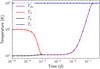Fig. 1 0D test of our three-temperature scheme, for which we set the dust-gas stopping time ts = 10−9t0 = 8 × 10−9 d and the opacity κd = 3.9 cm2g−1. Pluses indicate numerical results, while solid lines indicate analytical solutions taken from Eqs. (21) (red, black) and (24) (purple). Because the system is dominated by radiation energy, the radiation temperature (blue) is nearly constant throughout the system’s evolution.

3.2 1D test: Subcritical dusty radiative shock

Having verified that our scheme accurately reproduces three-temperature static thermal coupling, we seek to study its performance in a a dynamical setting. To this end, we ran a modified version of the 1D subcritical radiative shock in Ensman (1994), a standard test for radiation-hydrodynamic codes (see e.g., Sect. 4.1 of Melon Fuksman et al. 2021, and references therein) incorporating sharp transitions in temperature and opacity.

In this setup, our domain spans the interval [0,7 × 10¹⁰ cm]. The initial gas density is ρ_g = 7.78 × 10⁻¹⁰ g cm⁻³, with a dust-to-gas ratio f_d = 10⁻². Dust, gas, and radiation temperatures are all initialized in equilibrium, T_r = T_g = T_d = 10 K; γ = 7/5, µ = 1, and c_d = c_g are the same as in the 0D case. The dust absorption opacity is set such that the inverse mean free path of radiation through dust, $l_{\text{d}}^{-1}\equiv {\kappa }_{\text{d}}{\rho }_{\text{d}}=3.1\times {10}^{-10}{\text{cm}}^{-1}$, with dust scattering opacity of χ_d − κ_d, and a gas total opacity of χ_g, both assumed to be zero. To form the shock, given our otherwise equilibrium initial conditions, we set an initial gas velocity υ_x = −6 km s⁻¹ and imposed a reflective condition on the left boundary. We fiducially chose a reduced speed of light ĉ = 10⁻³ c and a spatial resolution N_x = 1200 cells. These figures give results that are consistent with those of our tests (not shown) at ĉ = c, and both higher and lower resolutions.

We tested stopping times, t_s = {10⁻⁷,10⁻⁴,10⁻¹ }t₀, where we again used t₀ = 8 d as the code unit for time. For this problem, we define the characteristic timescale using l_d as our length scale and υ_x as the velocity scale, yielding t_cross = 7.78 × 10⁻²t₀ and t_s/t_cross = 1.28 × {10⁻⁵,10⁻²,10¹}. The last case is included to demonstrate the properties of our code when dust and gas have weak thermal coupling, although the long t_s/ t_cross would also allow for relative motion between dust and gas, which we did not model.

In Fig. 2, we plot temperature snapshots at t = 0. 054t₀ = 3.75 × 10⁴ s for all stopping times, selecting N_x = 1200 as our fiducial resolution. For t_s = 10⁻¹, the gas temperature is that of a standard hydrodynamic shock. In the pre-shock region, dust and gas are essentially in equilibrium; in the post-shock region, by contrast, the dust heats at a rate ${\dot{T}}_{\text{d},\text{coll}}\approx \left(T_{\text{g}}-T_{\text{d}}\right)t_{\text{c},\text{dust}}^{-1}\approx \left(T_{\text{g},+}-T_{\text{d},-}\right)t_{\text{c},\text{dust}}^{-1}$, where minuses and pluses denote pre- and post-shock quantities, respectively. Deeper in the post-shock region, this trend breaks down, as radiative cooling (which scales as ${\dot{T}}_{\text{d},\text{rad}}\approx -c{l}_{\text{d}}^{-1}{a}_{\text{r}}\left(T_{d,-}^4-T_{r,-}^4\right)/c_{\text{d}}{\rho }_{\text{d}}$) becomes sufficient to counteract the effects of collisional heating.

In the t_s = 10⁻⁴t₀ case, the cooling time, t_c,dust, is short and T_d increases rapidly immediately after encountering the shock. Because the collisional heating rate is faster than for t_s = 10⁻¹t₀, the radiative cooling rate, and thus the maximum post-shock dust temperature, must be correspondingly higher. In the pre-shock region, this process is inverted: radiation propagating from the shock front heats the dust above its initial preshock value and, via collisions, the gas. For the strongly coupled case, with t_s = 10⁻⁷t₀, dust and gas are in collisional equilibrium, and we recover the two-temperature results of Melon Fuksman et al. (2021). Because the Courant-limited radiation timestep Δt_rad ≈ Δx/ĉ is much longer than our dust coupling time, this result demonstrates the efficacy of our IMEX scheme in the stiff regime.

In these 1D simulations, changes in the radiation field are driven by collisional heating of the dust, and ultimately by the rightward motion of the shock front in a process that s much slower than radiation propagation or absorption and emission. In this regime, we can drop the time derivative terms in Eq. (1f) and take the nonrelativistic limit of: $$\nabla \left(\text{Ξ}{E}_r\right)\approx -{\rho }_{\text{d}}{\kappa }_{\text{d}}{F}_x=-l_{\text{d}}^{-1}{F}_x,$$(25)

where the [I] parameter is defined in Eq. (9) as a function of the “reduced flux” w. Adding a sign to this reduced flux w_x = F_x/E_r = ±w and rearranging terms, we get: $${\partial }_{w_x}\left(\text{Ξ}\right)\nabla \left(w_x\right)\approx -\left(l_{\text{d}}^{-1}{w}_x+l_r^{-1}\text{Ξ}\right),$$(26)

where $l_r^{-1}\equiv \nabla \left(E_r\right)E_r^{-1}$ is the relative rate of change in the radiation field. In other words, variations in the radiation field on length scales shorter (longer) than some critical scale l_dΞ|w_x|⁻¹ drive (damp) the flux.

This is clearly visible in Fig. 2: in the t_s = 10⁻¹t₀ case, the relatively moderate gradient in radiation energy means that the transition from the w_x ≈ 0 diffusion regime to the w_x ≈ 1 free-streaming regime occurs smoothly over the post-shocked region. For s ≳ 5 × 10⁵ km, radiation from the shock front is sufficiently extincted, so the radiation field is dominated by the flat 10 K background; accordingly, |l_r| → ∞ and w_x damps to zero.

By contrast, the t_s = 10⁻⁷t₀ case has a flat radiation field for much of the post-shock region, but a sharper one in the immediate vicinity of the shock, creating an abrupt transition between the diffusion and free-streaming regimes. Because the post-shock radiation field is stronger in this case, it propagates to a greater optical depth before decaying into the flat T_r = 10 K background, so the w_x damping seen in the t_s = 10⁻¹t₀ simulation is not visible in the plotted region. The t_s = 10⁻¹t₀ case represents an intermediate case between these two extremes.

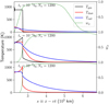Fig. 2 Temperature profiles in the dusty radiative shock test at t = 0.054t0 = 3.75 × 104 sec, for a variety of stopping times. For ts = 10−1, the gas temperature is that of a standard hydrodynamic shock, with only weak losses to dust and radiation; for ts = 10−7, Td, and Tg have come into equilibrium, and they (along with wx and Tr) match the results of the two-temperature radiative shock tests in Sect. 4.1 of (Melon Fuksman et al. 2021). We note that the signed “reduced flux” of wx = Fx/Er is denoted as f in their work.

3.3 2D test: Self-shadowing instability

The self-shadowing or thermal wave instability (SSI; see e.g., D’Alessio et al. 1999; Dullemond 2000; Watanabe & Lin 2008; Flock et al. 2020; Wu & Lithwick 2021) has been proposed as a planet-free means of generating gaps and rings in circumstellar disks. The SSI begins with a disk in initial radiative and (vertical) hydrostatic equilibrium. A small perturbation to the disk’s radial τ_r = 1 surface would create slightly raised regions that absorb more stellar irradiation, and lowered, obscured regions, which absorb less. To maintain hydrostatic equilibrium, the raised regions would increase in scale height (and thus absorb even more starlight), while the lowered ones would decrease in scale height and absorb even less.

The SSI is readily reproduced in 1+1D simulations that parametrize the vertical extent of a disk (e.g., Ueda et al. 2021). It can also be generated (e.g., Ueda et al. 2019) by an iterative procedure that first uses radiative transfer to obtain a disk’s temperature profile, given its density structure; assuming hydrostatic equilibrium, this profile is then used to recompute the density structure for the next iteration.

However, Melon Fuksman & Klahr (2022) found that this picture breaks down with additional physics: in their two-temperature radiation hydrodynamics simulations, the SSI bumps do not grow from noise and then they decay rapidly, even when artificially introduced via the aforementioned iterative procedure. They explain their results by arguing that the erosion of perturbations at the τ_r = 1 surface, caused by in-plane radiation transport and the hydrostatic adaptation of the gas in the upper disk, occurs on timescales that are much shorter than the classical vertical radiative heating timescale of the disk (Hubeny 1990; Zhu et al. 2015; Zhang & Zhu 2020), as in: $$t_{\text{SSI,rad}}=\frac{3\left({\tau }_{\upsilon }+{\tau }_{\upsilon }^{-1}\right)\left({\text{Σ}}_d{c}_{\text{d}}+{\text{Σ}}_{\text{g}}{c}_{\text{g}}\right)}{4c{a}_{\text{r}}\left(T_{\text{irr}}^2+T_{\text{d,mid}}^2\right)\left(T_{\text{irr}}+T_{\text{d,mid}}\right)},$$(27)

where ${\tau }_{\upsilon }={\kappa }_{\text{d}}\left({\text{Σ}}_d/2\right)$ is the vertical optical depth of the disk to the midplane in thermal infrared, Σ_d and Σ_g are the dust and gas surface densities, T_irr is the equilibrium temperature of the stellar irradiation field in the optically thin region of the disk, and T_d,mid is the dust midplane temperature. Physically, this means that bumps at the optical surface decay long before they can impact the temperature at the disk surface.

A nonzero coupling time between gas and dust temperatures would allow for a temperature perturbation at the τ_r = 1 surface to establish itself in the underlying disk column by propagating only through the dust; this is a much faster process than that implied via Eq. (27), in which the gas and dust are heated together. The subsequent adaptation of the gas’s vertical structure to this already-established background would conform better to the assumptions of iterative methods which have been successful in reproducing the SSI. Moreover, such a coupling time would delay the response of the perturbed τ_r = 1 gas to in-plane radiation transport, limiting the radial diffusion of SSI bumps. We emphasize that nothing about this prediction accounts for the effects of nonzero coupling times between dust and gas velocities on the evolution of the SSI. We defer this topic to a future work.

In the context of protoplanetary disks, a realistic coupling time may be found by computing t_s with the Epstein drag law (see e.g., Barranco et al. 2018; Speedie et al. 2022; Melon Fuksman et al. 2023) as follows: $$t_{\text{s}}=\frac{{\rho }_{\text{dg}}\langle a_{\text{dg}}^3\rangle }{{\rho }_{\text{g}}{\upsilon }_{\text{th}}\langle a_{\text{dg}}^2\rangle },$$(28)

where ρ_dg is the bulk density of each dust grain and ${\upsilon }_{\text{th}}=\sqrt{8\pi k_{\text{B}}{T}_{\text{g}}/\mu m_{\text{H}}}$ is the gas thermal velocity. A quantity in angle brackets 〈g(a_dg)〉 represents the integral of that quantity over the (normalized) grain size distribution n(a): $$\langle g\left(a_{\text{dg}}\right)\rangle ={\displaystyle {\int }_{a_{\min }}^{a_{\max }}g\left(a^{\prime }\right)n\left(a^{\prime }\right)\text{d}{a}^{\prime }.}$$(29)

For our three-temperature tests of the SSI, we used the setup dg3t100 from Melon Fuksman & Klahr (2022), generated with the aforementioned iterative procedure, as the basis for our initial conditions. We employ a reduced speed of light of ĉ = 10⁻³ c; our tests at ĉ′ = 5ĉ = 5 × 10⁻³ c (not shown) yielded converged results. The gas follows an ideal equation of state, with an adiabatic index of γ = 1.41 and a mean molecular weight of µ = 2.3. We assumed a total dust fraction of 1%, of which 10% by mass (f_d = 10⁻³) are taken to be small grains relevant to the gas’s thermal evolution. These grains were taken to consist of 62.5% silicate and 37.5% graphite, with a bulk density of ρ_gr = 2.5 g cm⁻³ and a specific heat capacity of c_d = 0.7 Jg⁻¹ K⁻¹; their sizes follow a classical MRN (Mathis et al. 1977) distribution, n(a) ∝ a^−3.5, with a_min = 5 nm and a_max = 250 nm².

From these grain properties, we computed a temperature-dependent, frequency-integrated dust opacity, κ_d(T_d), based on the tabulated frequency-dependent figures by Krieger & Wolf (2020, 2022) as well as t_s. We additionally bracketed the dust stopping time to lie within [10⁻¹⁰/2π, 10¹ /2π] years and took T_g → max(T_g, 10 K) for the purpose of computing υ_th. We assumed a classical T Tauri star with M_* = 1 M_⊙, R_* = 2.0865 R_⊙, and T_* = 4000 K, to compute the dust irradiation source term, S_d, as well as the gravitational potential: $${\text{Φ}}_{*}=-\frac{G{M}_{*}}{r_{*}},$$(30)

where r_* ≡ ‖x − x‖ is the distance between the star and a given point in the domain. We plot the resulting initial condition, as well as relevant contours for radial optical depth, τ_r, and gas cooling parameter, $\beta \equiv t_{\text{c}}\text{Ω=}\left(2/3\right)\left(\gamma -1\right)f_{\text{d}}^{-1}{t}_{\text{s}}\text{Ω}$, shown in the upper panel of Fig. 3. We emphasize that our yß-cooling parameter reflects only gas-grain collisions; because we self-consistently modeled the radiative transfer, we did not incorporate assumptions about time or length scales for radiative diffusion or optically thin cooling, as in some previous works (e.g., Bae et al. 2021).

We ran our SSI simulation in 2D axisymmetric polar coordinates, with radial limits at r = [0.4,100] au and polar limits at θ = π/2 + [−0.23,0.23]. This domain was spanned by {N_r, N_θ} = {512,170} grid cells, logarithmically spaced in the radial direction and uniformly spaced in polar angle. At the boundaries, all fields were set equal to those in dg3t0.1, the fiducial smooth hydrostatic setup in Melon Fuksman & Klahr (2022). We also included a damping zone in the region {r < r_damp,in} ∪ {p < 0}, where r_damp,in = 0.5 au and p ≡ −|θ − π/2| + 0.12 + 0.13(r/au). In this zone, we enforced T_d = T_g, while relaxing ρ and υ to their smooth hydrostatic values on a timescale of: $$t_{\text{damp}}=0.1\text{Ω}{\left(r\right)}^{-1}{\cos }^2\left[\pi /2\left(1+p/p_{+}\right)\right],$$(31a)

in the region where s < 0, and $$t_{\text{damp}}=0.1\text{Ω}{\left(r\right)}^{-1}{\cos }^{-2}\left[\pi /2\left(\frac{r-r_{\text{in}}}{r_{\text{damp,in}}-r_{\text{in}}}\right)\right],$$(31b)

elsewhere in the damping zone; we have tested alternative damping prescriptions and found no substantive change to our results. For comparison with the two-temperature regime, we also ran a simulation with a fixed global stopping time of t_s = (2π)⁻¹ × 10⁻¹⁰ yr, but otherwise identical.

In Fig. 4, we plot T_d and T_g from our realistic three-temperature simulation, as well as the matter temperature, T_ref, in the two-temperature reference simulation, at t = {0, 1, 10, 100} y. In the reference simulation, the initial scale-height perturbations at the τ_r = 1 surface dissipate rapidly and are almost completely absent by t = 10 y, reproducing the results of the equivalent two-temperature runs in Melon Fuksman & Klahr (2022). Our three-temperature realistic simulation, in which ß ≈ 1 at the τ_r = 1 surface, shows a similar evolution, as T_g still evolves too fast to achieve the smooth, columnar hydrostatic adaptation obtained in 1+1D and iterative approaches that reproduce the SSI. To better understand this temperature evolution, we plot in Fig. 5 the time evolution of T_d, T_g, and T_ref – normalized by the final, relaxed reference temperature T_relax, in a fiducial disk column at r = 2 au.

By t = 10² yr, the temperature profile within the τ_r = 1 surface of the realistic simulation has largely reached the same smooth equilibrium as in the reference. The slow-cooling disk atmosphere in the realistic case, heated by waves emitted by the disk’s initial relaxation and reflecting off the boundaries, is too low in density and optical depth to substantively alter this picture. It remains an open question as to what extent three-temperature methods can sustain the SSI. In this regard, our numerical experiments with a dust-gas coupling time artificially increased by 100× (described in Appendix B) show some promise, allowing SSI waves to survive and propagate inward for roughly ~10² yr before decaying.

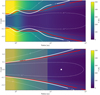Fig. 3 Initial Td = Tg for our 2D self-shadowing test Sect. (3.3), based on dg3t100 from Melon Fuksman & Klahr (2022), shown above, and the same for our 3D planet-driven spiral test Sect. (3.4), based on dg3t0.1, shown below. We overplot the contours for the radial optical depth, τr, in red (computed using opacities Planck-averaged over the stellar spectrum) and cooling parameter of β = tcΩ. Our calculations of these quantities assume an MRN distribution of small silicon-graphite grains and a 1M⊕ classical T Tauri star as the source of light and gravity. In the lower plot, a white dot indicates the position of the embedded 1 MJ planet, while grey shading covers the region outside the r = [8,100] au boundaries of our 3D simulation.

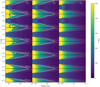Fig. 4 2D temperature profiles from our SSI tests. The Tg (left) and Td (middle) columns come from our simulations with realistic ts, whereas Tref (right) is from our reference simulations with ts = (2π)−1 × 10−10 yr. For ease of interpretation, we overplot β = 1 (white) and τ = 1 (red) surfaces. The reference disk relaxes rapidly to a smooth hydrostatic configuration; the bulk of the realistic disk does so as well, although differences persist in the slowly-cooling disk atmosphere.

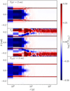Fig. 5 Time evolution of Td (top), Tg (center), and Tref (bottom) in a disk column at the fiducial r = 2 au, as compared to the final, relaxed state of Tref. As in Fig. 4, we plot the τr = 1 optical surface in red and the ß = 1 cooling surface in white. Tref, as well as Td and Tg, rapidly relax to a smooth equilibrium disk inside the ß = 1 surface. Sound waves in the upper atmosphere, excited by the initial relaxation of the disk, are visible in Tg due to the slow cooling rate at high altitude.

3.4 3D test: Planet-driven spirals

In recent years, high-resolution observations in NIR (e.g., Benisty et al. 2015; Wagner et al. 2019; Xie et al. 2021) and in various molecular lines (e.g., Teague et al. 2019; Wölfer et al. 2021) have revealed spiral structures in circumstellar disks. It is hypothesized that some fraction of these are driven by embedded, planetary-mass companions (Goldreich & Tremaine 1978, 1979, 1980; Goodman & Rafikov 2001).

Early simulations of these spirals (e.g., Kley 1999) often used 2D, vertically averaged setups, with a locally isothermal equation of state. Subsequent advances in computational power made it feasible to run disk-planet interaction simulations in full 3D (e.g., Fung & Dong 2015; Dong et al. 2016), relax the assumption of local isothermality (Zhu et al. 2015), and implement realistic vertical temperature structures (Juhász & Rosotti 2018); these, in turn, have enabled meaningful comparisons of simulated spirals to observations in dust (Dong & Fung 2017) and gas (Muley et al. 2021). More recently, Bae et al. (2021) used a parametrized cooling prescription to include the effects of matter-radiation interaction and gas-grain collisions. In what follows, we build on these previous works by modeling spirals with self-consistent, three-temperature radiation hydrodynamics.

For this test, we use the relaxed hydrostatic setup dg3t0.1 from Melon Fuksman & Klahr (2022) as a starting point. The dust properties, stellar parameters, and cooling prescription are the same as those in Sect. 3.3, and we plot our initial condition, as well as the resulting contours for ß and τ_r, in the lower panel of Fig. 3. For this test, we assumed ĉ = 10⁻⁴c. Our simulation was run in 3D spherical coordinates, with radial boundaries at r = [8,100] au, polar boundaries at θ = π/2 + [−0.27,0.27], and azimuthal boundaries at ϕ = [0,2π]; this simulation box is covered by {N_r, N_θ, N_ϕ} = {234,54,583} cells, logarithmic in radius and uniform in azimuthal and polar angle. All fields are fixed to their initial values at the radial and azimuthal boundaries, and periodic at the azimuthal boundary.

In addition to the star and its gravitational potential, Φ_*, our simulation includes a q ≡ M_p/M_* = 10⁻³ planet (M_p ≈ 1.05M_J), fixed on a circular Keplerian orbit with semimajor axis a_p = 20 au; at this radius, our temperature profile implies a disk aspect ratio (h/r)_p = 0.057 and a q_th = 5.5 times the thermal mass. The planetary potential is given, following Klahr & Kley (2006), by $${\text{Φ}}_p=-\frac{G{M}_p}{r_p}\{\begin{array}{cc}1& \text{if\hspace{0.17em}\hspace{0.17em}}{r}_p\ge r_s\\ \left({\left[r_p/r_s\right]}^4-2{\left[r_p/r_s\right]}^3+2\left[r_p/r_s\right]\right)& \text{if\hspace{0.17em}\hspace{0.17em}}{r}_p<r_s\end{array},$$(32)

where r_p ≡ ‖x − x_p‖ is the distance between the planet and a point in our domain, and r_s is the smoothing length, implemented to avoid a singularity in the potential. In our simulations, we set r_s = r_H/2.

To avoid unphysically shocking the disk at early times, we introduced this companion at t_i = 1 yr and grew it from zero to its final mass over the following t_grow = 10 yr. We solved our equations in the planet’s co-rotating frame, fixing its azimuthal coordinate as ϕ_p = π/4. In this frame, the pattern speed of the spiral, and consequently of the non-axisymmetric radiation field, is zero; deviations would be on the order of c_s ≈ 10⁻⁶c ≈ 10⁻²ĉ. Numerical tests at ĉ′ = 2 × 10⁻⁵ = ĉ/5, not shown here, yield a well-converged spiral amplitude. To prevent the growth of large-scale disk instabilities such as the Rossby wave instability (RWI; Lovelace & Romanova 2014), we included a kinematic viscosity $v=\alpha c_s^2{\text{Ω}}^{-1}$, where α = 0.001 is the Shakura & Sunyaev (1973) viscosity parameter. As in Sect. 3.3, we ran a three-temperature realistic simulation, as well as an otherwise-identical reference simulation with t_s = (2π)⁻¹ × 10⁻¹⁰ yr.

To keep the focus on the spirals, we analyzed the snapshot at t_cut = 500 yr, before our super-thermal planet has had the chance to carve a gap in the disk. In Fig. 6, we present the gas densities in our three-temperature realistic (ρ_gas) and two-temperature reference (ρ_ref) simulations, taken at r = 30 au and θ = {0,0.15,0.2}. At θ = 0, the primary and secondary Lindblad spirals are visible in both ρ_gas and ρ_ref, and agree to within several percent. This is expected because the three-temperature mid-plane value ß ≲ 10⁻² and reference simulation global value ß ≲ 10⁻¹¹ are both much shorter than the spiral-crossing timescale, β_sprial ≈ (h/r)|1 − Ω_p/Ω₃₀|⁻¹ (Sturm et al. 2020), where Ω₃₀ is the Keplerian frequency at 30 au. In the upper disk, the realistic ß ≈ 1 exceeds /ß_spiral, while the reference ß remains unchanged. Due to this difference in the thermal physics, the density structures become discrepant at the ~20% level, with Lindblad spirals being more sharply defined in ρ_ref than in ρ_gas.

In Fig. 7, we plot temperatures at the same cuts studied in Fig. 6. In the midplane of our three-temperature simulation, strong dust-gas coupling ensures that T_d and T_g are equal. At θ = 0.15, dust-gas coupling is somewhat weaker, with a ß ≈ 10⁻¹ ≈ ß_spiral, and differences between T_d and T_g are visible throughout the azimuthal extent of our cut. High in the disk atmosphere, at θ = 0.2, the normalized cooling time is ß ≈ 1, much longer than the spiral-crossing timescale for gas. Here, we observe a spiral feature in T_g with an amplitude ~10%, which is comparable to that found the ß = 1, M_p = 400 M_⊕ spiral simulation in Muley et al. (2021), but is not visible in T_d or T_ref.

At θ = 0, we observe a slight temperature dip centered at ϕ = ϕ_p = π/4, while at θ = 0.15 and θ = 0.2, we find a temperature bump at the same azimuthal position. This is ultimately caused by the gravitational influence of the planet, which lowers the τ_r = 1 surface overhead and thus changes the illumination of material in the radial band ϕ ≈ ϕ_p, r ≳ r_p. Such a feature was also observed in the Monte Carlo radiative transfer post-processing of Muley et al. (2021)’s hydrodynamical simulations.

To provide a more visual understanding of these results, we present 2D polar cuts of T_d, T_g, and T_ref at θ = 0.0 and θ = 0.2 in Fig. 8. We find, as in our 1D quantitative plots, that the morphology of T_ref largely agrees with that of T_d, despite substantial differences in ß between and within each simulation, while T_g and T_d only agree with one another when ß < ß_spiral. We interpret this to imply that T_d is set by the very short timescales for the dust's collisional energy exchange $t_{\text{c,dust}}=r_{\text{gd}}^{-1}{t}_c$ (following Eq. (6)) and for radiative cooling, either vertically or in-plane (Miranda & Rafikov 2020a; Ziampras et al. 2020). How T_g, in turn, reacts to the dust depends on the much longer local gas cooling time t_c = ß/Ω. This a result that could affect the observational signatures disk-planet interaction produces in gas and dust. We note, in addition, a slight discrepancy between the background T_dust and T_ref, with the latter being systematically lower throughout the disk; this is because spirals are more vertically extended in the two-temperature limit, and so cast stronger shadows throughout the disk. We intend to investigate these issues further in a future study.

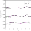Fig. 6 Density values for our three-temperature realistic (ρgas) and reference (ρref) simulations, taken at the indicated θ values at a fixed r = 30 au. Densities largely agree to within a few percent between both models, but the discrepancy rises to ~20% at the τr = 1 surface, causing a mild impact on the temperature structure below.

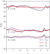Fig. 7 Temperatures in our three-temperature realistic (Tgas, Tdust) and reference (Tref) simulations, taken at the same cuts as in Fig. 6. In the midplane, where coupling times are short, Tgas = Tdust, but in the disk atmosphere, where coupling is weaker, there is a noticeable (~10%) discrepancy between the two: Tdust reflects the stellar irradiation field, while Tgas is driven by the PdV work done by the planetary spiral.

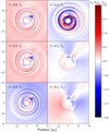Fig. 8 Relative difference between the temperature at tcut = 500 yr and the initial profile, in polar cuts at θ = 0.0 and θ = 0.2. The morphology of Td and Tg agree in the midplane, but diverge at higher altitude, while the morphology of Td and Tref agree everywhere. In each panel, we indicate the Hill sphere of the planet with a small solid grey circle, and our cuts in Figs. 6 and 7 with a large dotted grey circle.

4 Conclusion

We have developed an implicit-explicit (IMEX) numerical scheme for the PLUTO hydrodynamics code to self-consistently model energy exchange between gas, dust, and radiation. The implicit substep, consisting of nonrelativistic matter-radiation interaction source terms, is solved iteratively with a multidimensional Newton-Raphson method, whereas the explicit substep, consisting of radiation transport and relativistic interaction source terms, is solved using a Godunov scheme, following Melon Fuksman & Mignone (2019). Because this explicit part is Courant-limited, we use the reduced speed of light approximation, as implemented by Melon Fuksman et al. (2021), to improve computational efficiency. This gives physically reasonable results, so long as the reduced speed of light ĉ is much higher than all other relevant velocities in the problem.

In our 0D matter-radiation coupling test, we demonstrate the ability of our scheme to reproduce the “two-temperature” regime of traditional radiation hydrodynamics, where dust and gas are well-coupled. For the 1D Ensman (1994) shock tube test, we relax this assumption and investigate the behavior of gas, dust, and radiation temperatures in different coupling regimes. Our subsequent tests illustrate the applicability of three-temperature radiation hydrodynamics to active problems in circumstellar disk research, including realistic opacities and dust-gas coupling times computed from local temperature and density. Our 2D test shows that the self-shadowing instability, which arises in 1+1D time-dependent models with parametrized disk scale height, as well as 2D iterative techniques that alternate the calculation of radiative and hydrostatic equilibrium, decays rapidly in the two-temperature limit; this is also the case with realistic three-temperature coupling times, in line with previous expectations (Melon Fuksman & Klahr 2022). However, an increased cooling time (Appendix B) allows for dust temperatures in most of the disk column to rapidly adapt to stellar irradiation before the gas can react, which better satisfies the key assumptions of the aforementioned iterative and 1D hydrostatic methods, and so allows SSI-type scale-height perturbations to survive for somewhat longer before decaying. In our 3D spiral simulations, dust temperatures are remarkably consistent between the two- and three-temperature regimes, but gas temperatures disagree in the upper atmosphere. This is a result that carries certain implications for observations of spirals in gas tracers such as ¹²CO. Future potential applications of our three-temperature scheme include studies of circumplanetary disk accretion shocks, planetary gap opening, photoevaporation, and hydrodynamic or MHD instabilities such as the vertical shear instability, among many others.

Our scheme makes the simplifications that dust and gas move at the same velocity, and that dust inertia is negligible (St ≡ t_sΩ ≪ 1, ƒ_d ≪ 1). While these are reasonable assumptions for the sub-µm grains that supply most of a disk’s total opacity and set its overall thermal structure, they are invalid for the millimeter grains that concentrate at pressure maxima and produce much of its continuum emission. Including such grains would require accounting for multispecies momentum transfer including back-reaction from the gas (using schemes such as those detailed in e.g., Benítez-Llambay et al. 2019; Huang & Bai 2022) and thermal coupling. While such a method would be immensely helpful in interpreting continuum observations of gaps, rings, and spirals, it would be computationally demanding and require extensive testing beyond the scope of this work.

Acknowledgements

We thank Remo Burn, Cornelis Dullemond, Mario Flock, Thomas Henning, Carolin Kimmig, Giancarlo Mattia, Thomas Rometsch, and Prakruti Sudarshan for useful discussions. We are also grateful to the anonymous referee, whose report helped improve the quality of this paper. All numerical simulations were performed on the Cobra cluster of the Max Planck Society and the Vera Cluster of the Max Planck Institut für Astronomie, both hosted by the Max Planck Computing and Data Facility (MPCDF) in Garching bei München. The research of J.D.M.F. and H.K. is supported by the German Science Foundation (DFG) under the priority program SPP 1992: “Exoplanet Diversity” under contract KL 1469/16-1/2.

Appendix A Newton-Raphson iterations

We rearrange Equations 18a and 18b as a vector of quantities $P\left({\xi }_{\text{sub}}^{i+1}\right)\equiv {\left(P_d,P_g\right)}^{\top }$, where ${\xi }_{\text{sub}}^{i+1}\equiv \left({\xi }_{\text{d}}^{i+1},{\xi }_{\text{g}}^{i+1}\right)$. Thus we obtain: $$\begin{array}{l}{P}_d={\xi }_{\text{d}}^i-{\xi }_{\text{d}}^{i+1}-{\left(t_{\text{c}}^{i+1}\right)}^{-1}\left[r_{\text{gd}}{\xi }_{\text{d}}^{i+1}-{\xi }_{\text{g}}^{i+1}\right]\delta t\hfill \\ -c\rho {\kappa }_{\text{d}}^{i+1}{f}_{\text{d}}\left[a_{\text{r}}{\left(T_{\text{d}}^{i+1}\right)}^4-{\xi }_{\text{r}}^{i+1}\right]\delta t+S{}_d\delta t\hfill \end{array},$$(A.1) $$\begin{array}{l}{P}_{\text{g}}={\xi }_{\text{g}}^i-{\xi }_{\text{g}}^{i+1}+{\left(t_{\text{c}}^{i+1}\right)}^{-1}\left[r_{\text{gd}}{\xi }_{\text{d}}^{i+1}-{\xi }_{\text{g}}^{i+1}\right]\delta t\hfill \\ -c\rho {\kappa }_{\text{g}}^{i+1}\left[a_{\text{r}}{\left(T_{\text{g}}^{i+1}\right)}^4-{\xi }_{\text{r}}^{i+1}\right]\delta t+S{\text{\hspace{0.17em}g}}_{}\delta t\hfill \end{array},$$(A.2)

where $${\xi }_{\text{r}}^{i+1}={\xi }_{\text{r}}^i-\frac{\widehat{c}}{c}\left[\left({\xi }_{\text{d}}^{i+1}-{\xi }_{\text{d}}^i\right)+\left({\xi }_{\text{g}}^{i+1}-{\xi }_{\text{g}}^i\right)\right].$$(A.3)

Using Newton's method, we attempt to find a vector ξ^i+1,*, such that P(ξ^i+1,*) = 0 to within some small tolerance α. The relevant Jacobian matrix J(ξⁱ⁺¹) ≡ ∂P/∂ξ^i+l is: $$J\left({\xi }_{\text{sub}}^{i+1}\right)=\left[\begin{array}{ll}\partial P_d/\partial {\xi }_{\text{d}}^{i+1}\hfill & \partial P_d/\partial {\xi }_{\text{g}}^{i+1}\hfill \\ \partial P_{\text{g}}/\partial {\xi }_{\text{d}}^{i+1}\hfill & \partial P_g/\partial {\xi }_{\text{g}}^{i+1}\hfill \end{array}\right],$$(A.4) $$\partial P_d/\partial {\xi }_{\text{d}}^{i+1}=-\left(1+r_{\text{gd}}\delta t/t_{\text{c}}^{i+1}\right)-c\rho {\kappa }_{\text{d}}^{i+1}{f}_{\text{d}}\delta t\left[4a_{\text{r}}\left(T_{\text{d}}^{i+1}\right)/\rho f_{\text{d}}{c}_{\text{d}}+\widehat{c}/c\right],$$(A.5) $$\partial P_d/\partial {\xi }_g^{i+1}=+\delta t/t_{\text{c}}^{i+1}-\widehat{c}\rho {\kappa }_{\text{d}}^{i+1}{f}_{\text{d}}\delta t,$$(A.6) $$\partial P_g/\partial {\xi }_{\text{d}}^{i+1}=+r_{\text{gd}}\delta t/t_{\text{c}}^{i+1}-\widehat{c}\rho {\kappa }_g^{i+1}\delta t,$$(A.7) $$\partial P_g/\partial {\xi }_{\text{g}}^{i+1}=\left(1+\delta t/t_{\text{c}}^{i+1}\right)-c\rho {\kappa }_g^{i+1}\delta t\left[4a_{\text{r}}{\left(T_{\text{g}}^{i+1}\right)}^3/\rho c_g+\widehat{c}/c\right].$$(A.8) $$J\left({\xi }_n^{i+1}\right)\left[{\xi }_{n+1}^{i+1}-{\xi }_n^{i+1}\right]=-P_n,$$(A.9)

where n is an iteration index, in contrast to the timestep index i.

Appendix B Self-shadowing instability with long coupling times

Our investigation in Section 3.3 found that, just as in the two-temperature case, our “realistic” three-temperature disk with self-consistently evaluated dust-gas coupling times cannot sustain the self-shadowing instability (SSI). This result, however, leaves open the question of whether there is any circumstance under which three-temperature dynamics could favor the survival of the SSI. To study this possibility, we ran a simulation with dust-gas coupling times 100× larger than those in the realistic run in Section 3.3. To facilitate comparison with our previous results, we hold all other simulation parameters (including, crucially, the dust opacity prescription and dust-to-gas ratio) fixed. Formally, solving for t_s in Equation 5, this would imply a Stokes number St ≈ 0.06 for grains at the τ_r = 1 surface, which can be expected to experience vertical drift. However, we emphasize that this 100×-cooling setup is artificial, and is designed to approximate and long relaxation times that arise in disk upper atmospheres in detailed calculations of grain growth, settling, and depletion (see e.g., Bae et al. 2021, for one such scenario). The dust populations arising from these calculations are, by construction, in steady state, and do not experience net vertical drift.

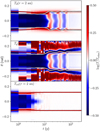Fig. B.1 Plot similar to our Figure 5, but with Td and Tg taken from our simulation with cooling times artificially raised by a factor of 100. There are clear vertical patterns in the dust and gas temperature profiles, corresponding to inward-traveling perturbations at the τr = 1 surface characteristic of the SSI.

In Figure B.1, we plot the time evolution of T_d, T_g, and T_ref normalized by the final, relaxed reference temperature T_relax in a fiducial disk column at r = 2 au. In the two-temperature reference simulation, the initialized self-shadowing perturbations rapidly decay (as already evident from Figure 4), but in the three-temperature 100× realistic simulation, they survive for some time, as evidenced by the vertical bands in T_d and T_g between t = 10¹ − 10² y.

At the leading edge of a self-shadowing scale-height perturbation, the flaring angle of the τ_r = 1 is high and intercepts more direct stellar irradiation. Although T_d reflects this change immediately, the fact that ß ≫ 1 in this disk region means that the response of T_g (and the consequent vertical expansion of the gas column to seek hydrostatic equilibrium) is significantly slower. As the gas column puffs up, it creates a new leading edge immediately to its interior; when this edge puffs up in turn, it blocks stellar irradiation from reaching the original column, causing it to cool and shrink. In this fashion, self-shadowing waves can propagate inward towards the star purely through vertical motions of the fluid elements. This mechanism would not operate when dust and gas are well-coupled; in that regime, both components would have a common temperature, and would respond to surface perturbations via layered radiative diffusion. The long timescale for this diffusion (given very roughly by Equation 27) means that surface perturbations would decay before having an effect deep in the disk (Melon Fuksman & Klahr 2022).

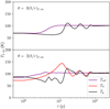Fig. B.2 Quantitative time evolution of Td and Tg from the 100×-realistic simulation, and Tref in the reference simulation, at r = 2 au, both in the midplane (θ = 0, above) and three scale heights above it (θ ≈ 0.088, below). As qualitatively shown in Figure B.1, Tref reaches a smooth equilibrium, whereas Td and Tg exhibit damped oscillations due to the passage of self-shadowing waves. See text for more details.

For a more quantitative view, we present in Figure B.2 the time evolution of T_d, T_g, and T_ref at r = 2 au and θ = π/2 + {0.0,0.088} (the latter θ corresponding to three scale heights above the midplane). At both altitudes, Tref relaxes almost immediately to its hydrostatic equilibrium value, where it remains for the rest of the simulation. The evolution of T_d and T_g is more complex. High in the disk, the dust temperature rises interior to self-shadowing bumps, and drops exterior to them; with some delay due to gas cooling parameters ß ≈ 1, we see that T_d relaxes toward T_g and the interior and exterior gas columns adapt to the new hydrostatic equilibrium. The net result, as mentioned earlier and in line with typical expectations for the SSI, is the apparent inward propagation of self-shadowing bumps. The changes these bumps make to the disk’s illumination profile impact the midplane temperature, albeit with some delay and attenuation due to radiative diffusion.

In Figure B.3, we present snapshots of the full long-coupling disk at selected times. Puffed-up disk columns heated above the background temperature, a hallmark signature of self-shadowing waves, are clearly visible here. They are captured n Figures B.1 and B.2 as they travel inward through r = 2 au. By t = 250 y, however, the long-cooling disk has largely relaxed to the same smooth equilibrium as the reference disk. Differences persist in the very slowly-cooling disk atmosphere, as well as in the r ≲ 1 au region in the immediate vicinity of our fixed inner radial boundary.

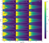Fig. B.3 Evolution of the SSI with a dust-gas coupling time 100× longer than in the self-consistent setup presented in 3.3. An inward-propagating SSI bump is clearly visible. At t = 250 y, the disk has largely relaxed to the same configuration as in the reference simulation. Differences do persist, however, outside the ß = 1 surface and near the inner boundary.

References

All Figures

Fig. 1 0D test of our three-temperature scheme, for which we set the dust-gas stopping time ts = 10−9t0 = 8 × 10−9 d and the opacity κd = 3.9 cm2g−1. Pluses indicate numerical results, while solid lines indicate analytical solutions taken from Eqs. (21) (red, black) and (24) (purple). Because the system is dominated by radiation energy, the radiation temperature (blue) is nearly constant throughout the system’s evolution.

In the text

Fig. 2 Temperature profiles in the dusty radiative shock test at t = 0.054t0 = 3.75 × 104 sec, for a variety of stopping times. For ts = 10−1, the gas temperature is that of a standard hydrodynamic shock, with only weak losses to dust and radiation; for ts = 10−7, Td, and Tg have come into equilibrium, and they (along with wx and Tr) match the results of the two-temperature radiative shock tests in Sect. 4.1 of (Melon Fuksman et al. 2021). We note that the signed “reduced flux” of wx = Fx/Er is denoted as f in their work.

In the text

Fig. 3 Initial Td = Tg for our 2D self-shadowing test Sect. (3.3), based on dg3t100 from Melon Fuksman & Klahr (2022), shown above, and the same for our 3D planet-driven spiral test Sect. (3.4), based on dg3t0.1, shown below. We overplot the contours for the radial optical depth, τr, in red (computed using opacities Planck-averaged over the stellar spectrum) and cooling parameter of β = tcΩ. Our calculations of these quantities assume an MRN distribution of small silicon-graphite grains and a 1M⊕ classical T Tauri star as the source of light and gravity. In the lower plot, a white dot indicates the position of the embedded 1 MJ planet, while grey shading covers the region outside the r = [8,100] au boundaries of our 3D simulation.

In the text

Fig. 4 2D temperature profiles from our SSI tests. The Tg (left) and Td (middle) columns come from our simulations with realistic ts, whereas Tref (right) is from our reference simulations with ts = (2π)−1 × 10−10 yr. For ease of interpretation, we overplot β = 1 (white) and τ = 1 (red) surfaces. The reference disk relaxes rapidly to a smooth hydrostatic configuration; the bulk of the realistic disk does so as well, although differences persist in the slowly-cooling disk atmosphere.

In the text

Fig. 5 Time evolution of Td (top), Tg (center), and Tref (bottom) in a disk column at the fiducial r = 2 au, as compared to the final, relaxed state of Tref. As in Fig. 4, we plot the τr = 1 optical surface in red and the ß = 1 cooling surface in white. Tref, as well as Td and Tg, rapidly relax to a smooth equilibrium disk inside the ß = 1 surface. Sound waves in the upper atmosphere, excited by the initial relaxation of the disk, are visible in Tg due to the slow cooling rate at high altitude.

In the text

	Fig. 6 Density values for our three-temperature realistic (ρgas) and reference (ρref) simulations, taken at the indicated θ values at a fixed r = 30 au. Densities largely agree to within a few percent between both models, but the discrepancy rises to ~20% at the τr = 1 surface, causing a mild impact on the temperature structure below.
In the text

Fig. 7 Temperatures in our three-temperature realistic (Tgas, Tdust) and reference (Tref) simulations, taken at the same cuts as in Fig. 6. In the midplane, where coupling times are short, Tgas = Tdust, but in the disk atmosphere, where coupling is weaker, there is a noticeable (~10%) discrepancy between the two: Tdust reflects the stellar irradiation field, while Tgas is driven by the PdV work done by the planetary spiral.

In the text

Fig. 8 Relative difference between the temperature at tcut = 500 yr and the initial profile, in polar cuts at θ = 0.0 and θ = 0.2. The morphology of Td and Tg agree in the midplane, but diverge at higher altitude, while the morphology of Td and Tref agree everywhere. In each panel, we indicate the Hill sphere of the planet with a small solid grey circle, and our cuts in Figs. 6 and 7 with a large dotted grey circle.

In the text

	Fig. B.1 Plot similar to our Figure 5, but with Td and Tg taken from our simulation with cooling times artificially raised by a factor of 100. There are clear vertical patterns in the dust and gas temperature profiles, corresponding to inward-traveling perturbations at the τr = 1 surface characteristic of the SSI.
In the text

Fig. B.2 Quantitative time evolution of Td and Tg from the 100×-realistic simulation, and Tref in the reference simulation, at r = 2 au, both in the midplane (θ = 0, above) and three scale heights above it (θ ≈ 0.088, below). As qualitatively shown in Figure B.1, Tref reaches a smooth equilibrium, whereas Td and Tg exhibit damped oscillations due to the passage of self-shadowing waves. See text for more details.

In the text

	Fig. B.3 Evolution of the SSI with a dust-gas coupling time 100× longer than in the self-consistent setup presented in 3.3. An inward-propagating SSI bump is clearly visible. At t = 250 y, the disk has largely relaxed to the same configuration as in the reference simulation. Differences do persist, however, outside the ß = 1 surface and near the inner boundary.
In the text

References

- Bae, J., Teague, R., & Zhu, Z. 2021, ApJ, 912, 56 [NASA ADS] [CrossRef] [Google Scholar]
- Barranco, J. A., Pei, S., & Marcus, P. S. 2018, ApJ, 869, 127 [NASA ADS] [CrossRef] [Google Scholar]
- Bate, M. R., & Keto, E. R. 2015, MNRAS, 449, 2643 [NASA ADS] [CrossRef] [Google Scholar]
- Benisty, M., Juhasz, A., Boccaletti, A., et al. 2015, A & A, 578, L6 [NASA ADS] [CrossRef] [EDP Sciences] [Google Scholar]
- Benítez-Llambay, P., Krapp, L., & Pessah, M. E. 2019, ApJS, 241, 25 [Google Scholar]
- Binkert, F., Szulágyi, J., & Birnstiel, T. 2023, MNRAS, 525, 4299 [NASA ADS] [CrossRef] [Google Scholar]
- Bitsch, B., Crida, A., Morbidelli, A., Kley, W., & Dobbs-Dixon, I. 2013, A & A, 549, A124 [NASA ADS] [CrossRef] [EDP Sciences] [Google Scholar]
- Bruderer, S. 2013, A & A, 559, A46 [NASA ADS] [CrossRef] [EDP Sciences] [Google Scholar]
- Bruderer, S., van Dishoeck, E. F., Doty, S. D., & Herczeg, G. J. 2012, A & A, 541, A91 [NASA ADS] [CrossRef] [EDP Sciences] [Google Scholar]
- Burke, J. R., & Hollenbach, D. J. 1983, ApJ, 265, 223 [NASA ADS] [CrossRef] [Google Scholar]
- Calahan, J. K., Bergin, E. A., Zhang, K., et al. 2021, ApJS, 257, 17 [NASA ADS] [CrossRef] [Google Scholar]
- Chiang, E. I., & Goldreich, P. 1997, ApJ, 490, 368 [Google Scholar]
- D'Alessio, P., Cantó, J., Hartmann, L., Calvet, N., & Lizano, S. 1999, ApJ, 511, 896 [CrossRef] [Google Scholar]
- Dong, R., & Fung, J. 2017, ApJ, 835, 38 [Google Scholar]
- Dong, R., Fung, J., & Chiang, E. 2016, ApJ, 826, 75 [Google Scholar]
- Dullemond, C. P. 2000, A & A, 361, L17 [NASA ADS] [Google Scholar]
- Dullemond, C. P., Hollenbach, D., Kamp, I., & D'Alessio, P. 2007, in Protostarsand Planets V, eds. B. Reipurth, D. Jewitt, & K. Keil (Tucson: University of Arizona Press), 555 [Google Scholar]
- Dullemond, C. P., Juhasz, A., Pohl, A., et al. 2012, Astrophysics Source Code Library [record ascl:1202.015] [Google Scholar]
- Ensman, L. 1994, ApJ, 424, 275 [NASA ADS] [CrossRef] [Google Scholar]
- Flock, M., Fromang, S., González, M., & Commerçon, B. 2013, A & A, 560, A43 [NASA ADS] [CrossRef] [EDP Sciences] [Google Scholar]
- Flock, M., Turner, N. J., Nelson, R. P., et al. 2020, ApJ, 897, 155 [Google Scholar]
- Fung, J., & Dong, R. 2015, ApJ, 815, L21 [NASA ADS] [CrossRef] [Google Scholar]
- Fung, J., Zhu, Z., & Chiang, E. 2019, ApJ, 887, 152 [NASA ADS] [CrossRef] [Google Scholar]
- Gnedin, N. Y., & Abel, T. 2001, New Astron., 6, 437 [NASA ADS] [CrossRef] [Google Scholar]
- Goldreich, P., & Tremaine, S. 1978, ApJ, 222, 850 [NASA ADS] [CrossRef] [Google Scholar]
- Goldreich, P., & Tremaine, S. 1979, ApJ, 233, 857 [Google Scholar]
- Goldreich, P., & Tremaine, S. 1980, ApJ, 241, 425 [Google Scholar]
- Goodman, J., & Rafikov, R. R. 2001, ApJ, 552, 793 [NASA ADS] [CrossRef] [Google Scholar]
- Hu, X., Li, Z.-Y., Wang, L., Zhu, Z., & Bae, J. 2023, MNRAS, 523, 4883 [NASA ADS] [CrossRef] [Google Scholar]
- Huang, P., & Bai, X.-N. 2022, ApJS, 262, 11 [NASA ADS] [CrossRef] [Google Scholar]
- Huang, S., & Yu, C. 2022, MNRAS, 514, 1733 [NASA ADS] [CrossRef] [Google Scholar]
- Hubeny, I. 1990, ApJ, 351, 632 [NASA ADS] [CrossRef] [Google Scholar]
- Juhász, A., & Rosotti, G. P. 2018, MNRAS, 474, L32 [Google Scholar]
- Keppler, M., Benisty, M., Müller, A., et al. 2018, A & A, 617, A44 [NASA ADS] [CrossRef] [EDP Sciences] [Google Scholar]
- Klahr, H., & Kley, W. 2006, A & A, 445, 747 [NASA ADS] [CrossRef] [EDP Sciences] [Google Scholar]
- Kley, W. 1999, MNRAS, 303, 696 [NASA ADS] [CrossRef] [Google Scholar]
- Kley, W., Bitsch, B., & Klahr, H. 2009, A & A, 506, 971 [NASA ADS] [CrossRef] [EDP Sciences] [Google Scholar]
- Krieger, A., & Wolf, S. 2020, A & A, 635, A148 [NASA ADS] [CrossRef] [EDP Sciences] [Google Scholar]
- Krieger, A., & Wolf, S. 2022, A & A, 662, A99 [NASA ADS] [CrossRef] [EDP Sciences] [Google Scholar]
- Levermore, C. D. 1984, J. Quant. Spec. Radiat. Transf., 31, 149 [NASA ADS] [CrossRef] [Google Scholar]
- Levermore, C. D., & Pomraning, G. C. 1981, ApJ, 248, 321 [NASA ADS] [CrossRef] [Google Scholar]
- Lovelace, R. V. E., & Romanova, M. M. 2014, Fluid Dyn. Res., 46, 041401 [NASA ADS] [CrossRef] [Google Scholar]
- Malygin, M. G., Klahr, H., Semenov, D., Henning, T., & Dullemond, C. P. 2017, A & A, 605, A30 [NASA ADS] [CrossRef] [EDP Sciences] [Google Scholar]
- Manger, N., Pfeil, T., & Klahr, H. 2021, MNRAS, 508, 5402 [NASA ADS] [CrossRef] [Google Scholar]
- Mathis, J. S., Rumpl, W., & Nordsieck, K. H. 1977, ApJ, 217, 425 [Google Scholar]
- Melon Fuksman, J. D., & Klahr, H. 2022, ApJ, 936, 16 [NASA ADS] [CrossRef] [Google Scholar]
- Melon Fuksman, J. D., & Mignone, A. 2019, ApJS, 242, 20 [NASA ADS] [CrossRef] [Google Scholar]
- Melon Fuksman, J. D., Klahr, H., Flock, M., & Mignone, A. 2021, ApJ, 906, 78 [NASA ADS] [CrossRef] [Google Scholar]
- Melon Fuksman, J. D., Flock, M., & Klahr, H. 2023, A & A, submitted [Google Scholar]
- Mignone, A., Bodo, G., Massaglia, S., et al. 2007, ApJS, 170, 228 [Google Scholar]
- Miranda, R., & Rafikov, R. R. 2019, ApJ, 878, L9 [NASA ADS] [CrossRef] [Google Scholar]
- Miranda, R., & Rafikov, R. R. 2020a, ApJ, 904, 121 [NASA ADS] [CrossRef] [Google Scholar]
- Miranda, R., & Rafikov, R. R. 2020b, ApJ, 892, 65 [NASA ADS] [CrossRef] [Google Scholar]
- Muley, D., Dong, R., & Fung, J. 2021, AJ, 162, 129 [NASA ADS] [CrossRef] [Google Scholar]
- Pareschi, L., & Russo, G. 2005, J. Sci. Comput., 25, 129 [MathSciNet] [Google Scholar]
- Pavlyuchenkov, Y. N., & Zhilkin, A. G. 2013, Astron. Rep., 57, 641 [NASA ADS] [CrossRef] [Google Scholar]
- Pavlyuchenkov, Y. N., Zhilkin, A. G., Vorobyov, E. I., & Fateeva, A. M. 2015, Astron. Rep., 59, 133 [CrossRef] [Google Scholar]
- Pierens, A., & Lin, M.-K. 2018, MNRAS, 479, 4878 [NASA ADS] [Google Scholar]
- Pinte, C., Teague, R., Flaherty, K., et al. 2022, arXiv e-prints [arXiv:2203.09528] [Google Scholar]
- Ren, B., Dong, R., Esposito, T. M., et al. 2018, ApJ, 857, L9 [Google Scholar]
- Shakura, N. I., & Sunyaev, R. A. 1973, A & A, 24, 337 [NASA ADS] [Google Scholar]
- Skinner, M. A., & Ostriker, E. C. 2013, ApJS, 206, 21 [NASA ADS] [CrossRef] [Google Scholar]
- Speedie, J., Booth, R. A., & Dong, R. 2022, ApJ, 930, 40 [NASA ADS] [CrossRef] [Google Scholar]
- Sturm, J. A., Rosotti, G. P., & Dominik, C. 2020, A & A, 643, A92 [NASA ADS] [CrossRef] [EDP Sciences] [Google Scholar]
- Tarczay-Nehéz, D., Regály, Z., & Vorobyov, E. 2020, MNRAS, 493, 3014 [CrossRef] [Google Scholar]
- Teague, R., Bae, J., Huang, J., & Bergin, E. A. 2019, ApJ, 884, L56 [Google Scholar]
- Ueda, T., Flock, M., & Okuzumi, S. 2019, ApJ, 871, 10 [Google Scholar]
- Ueda, T., Flock, M., & Birnstiel, T. 2021, ApJ, 914, L38 [NASA ADS] [CrossRef] [Google Scholar]
- Vorobyov, E. I., Matsukoba, R., Omukai, K., & Guedel, M. 2020, A & A, 638, A102 [CrossRef] [EDP Sciences] [Google Scholar]
- Wagner, K., Stone, J. M., Spalding, E., et al. 2019, ApJ, 882, 20 [Google Scholar]
- Wang, L., & Goodman, J. 2017, ApJ, 847, 11 [Google Scholar]
- Wang, L., Bai, X.-N., & Goodman, J. 2019, ApJ, 874, 90 [Google Scholar]
- Watanabe, S.-I., & Lin, D. N. C. 2008, ApJ, 672, 1183 [NASA ADS] [CrossRef] [Google Scholar]
- Whitney, B. A., Robitaille, T. P., Bjorkman, J. E., et al. 2013, ApJS, 207, 30 [Google Scholar]
- Woitke, P., Kamp, I., & Thi, W. F. 2009, A & A, 501, 383 [NASA ADS] [CrossRef] [EDP Sciences] [Google Scholar]
- Wölfer, L., Facchini, S., Kurtovic, N. T., et al. 2021, A & A, 648, A19 [CrossRef] [EDP Sciences] [Google Scholar]
- Wu, Y., & Lithwick, Y. 2021, ApJ, 923, 123 [NASA ADS] [CrossRef] [Google Scholar]
- Xie, C., Ren, B., Dong, R., et al. 2021, ApJ, 906, L9 [NASA ADS] [CrossRef] [Google Scholar]
- Yamaleev, N. K., & Carpenter, M. H. 2009, J. Comput. Phys., 228, 3025 [NASA ADS] [CrossRef] [Google Scholar]
- Zhang, S., & Zhu, Z. 2020, MNRAS, 493, 2287 [NASA ADS] [CrossRef] [Google Scholar]
- Zhu, Z., Dong, R., Stone, J. M., & Rafikov, R. R. 2015, ApJ, 813, 88 [Google Scholar]
- Ziampras, A., Kley, W., & Dullemond, C. P. 2020, A & A, 637, A50 [NASA ADS] [CrossRef] [EDP Sciences] [Google Scholar]