| Issue |
A&A
Volume 687, July 2024
|
|
|---|---|---|
| Article Number | A213 | |
| Number of page(s) | 22 | |
| Section | Planets and planetary systems | |
| DOI | https://doi.org/10.1051/0004-6361/202449739 | |
| Published online | 16 July 2024 | |
Three-temperature radiation hydrodynamics with PLUTO: Thermal and kinematic signatures of accreting protoplanets
Max-Planck-Institut für Astronomie,
Königstuhl 17,
Heidelberg
69117,
Germany
e-mail: muley@mpia.de
Received:
26
February
2024
Accepted:
3
May
2024
In circumstellar disks around young stars, the gravitational influence of nascent planets produces telltale patterns in density, temperature, and kinematics. To better understand these signatures, we first performed 3D hydrodynamical simulations of a 0.012 M⊙ disk with a Saturn-mass planet orbiting circularly in-plane at 40 au. We tested four different disk thermodynamic prescriptions (in increasing order of complexity: local isothermality, β cooling, two-temperature radiation hydrodynamics, and three-temperature radiation hydrodynamics), finding that β cooling offers a reasonable approximation for the three-temperature approach when the planet is not massive or luminous enough to substantially alter the background temperature and density structure. Thereafter, using the three-temperature scheme, we relaxed this assumption, simulating a range of different planet masses (Neptune-mass, Saturn-mass, and Jupiter-mass) and accretion luminosities (0 and 10−3 L⊙) in the same disk. Our investigation revealed that signatures of disk–planet interaction strengthen with increasing planet mass, with circumplanetary flows becoming prominent in the high-planet-mass regime. Accretion luminosity, which adds pressure support around the planet, was found to weaken the midplane Doppler flip, which is potentially visible in optically thin tracers such as C18O, while strengthening the spiral signature, particularly in upper disk layers sensitive to thicker lines, such as those of 12CO.
Key words: methods: numerical / protoplanetary disks / planet–disk interactions
© The Authors 2024
 Open Access article, published by EDP Sciences, under the terms of the Creative Commons Attribution License (https://creativecommons.org/licenses/by/4.0), which permits unrestricted use, distribution, and reproduction in any medium, provided the original work is properly cited.
This article is published in open access under the Subscribe to Open model.
Open Access funding provided by Max Planck Society.
1 Introduction
The high spectral and spatial resolution of the Atacama Large Millimeter Array (ALMA) have made it possible to accurately probe temperatures and velocities at the τ = 1 surfaces of various molecular lines, such as those associated with 12CO, 13CO, and C18O (Pinte et al. 2023b). Observations in systems such as HD 163296 (Pinte et al. 2018), HD 97048 (Pinte et al. 2019), TW Hya (Teague et al. 2019, 2022), CQ Tau (Wölfer et al. 2021), and Elias 2-24 (Pinte et al. 2023a) – with the background temperature and (sub-)Keplerian velocity profiles subtracted off -have revealed localized velocity kinks, as well as large-scale spiral structures in temperature and velocity. Numerical (e.g., Pérez et al. 2018) and analytical (e.g., Bollati et al. 2021) studies indicate that such signatures are consistent with those caused by spiral wakes (Goodman & Rafikov 2001) launched at Lind-blad resonances in the disk, where the Doppler-shifted planetary forcing frequency equals the local epicyclic frequency (e.g., Goldreich & Tremaine 1978, 1979).
For computational efficiency and ease of interpretation, simulations of disk–planet interaction have historically used a 2D, vertically integrated approach, with the gas following a locally isothermal equation of state. But as the quality of observations improve, it has become increasingly necessary to account for more detailed disk structure and thermodynamics in order to make a meaningful comparison. Zhu et al. (2012) and Lubow & Zhu (2014) simulated 3D adiabatic disks, discovering additional spirals excited at distinct buoyancy resonances, where the Doppler-shifted planetary forcing frequency equals the Brunt-Väisälä frequency. Lobo Gomes et al. (2015) simulated disk-planet interaction with cooling in 2D, running their simulations to gap-opening timescales with an emphasis on vortex formation at the outer pressure bump formed by the planetary gap. Zhu et al. (2015) performed global 3D simulations of planet-driven spirals with so-called β cooling, in which the temperature in a grid cell is relaxed to a preset background value (with β being the ratio of the cooling time to the local dynamical time,  ). Juhász & Rosotti (2018) performed 3D locally isothermal prescriptions, but with a vertically stratified temperature. Miranda & Rafikov (2020a,b) performed high-resolution, 2D simulations of spirals with β cooling, studying the details of angular momentum transport as cooling times varied from short (isothermal) to long (adiabatic) relative to the local dynamical time. The 3D simulations of Muley et al. (2021) incorporated β cooling along with a vertically stratified temperature structure obtained from radiative-transfer simulations, while Bae et al. (2021) went a step further and computed βcooling timescales at each point in the disk, based on radiative diffusion and gas–grain collision times. These studies conclude that Lindblad spirals propagate through the disk for β ≪ 1 (isothermal limit) or β ≪ 1 (adiabatic limit) but damp close to the planet location for β ≈ 1. Temperature stratification also causes the pitch angle and morphology of these spirals to deviate from the 2D, vertically averaged expectation, particularly at the high altitudes amenable to observations.
In addition to parametrized cooling, radiation-hydrodynamic techniques have also been used in the context of disk-planet interaction. A number of works have concentrated on planetary torques and migration (e.g., Kley et al. 2009; Lega et al. 2014; Fung et al. 2017; Chrenko & Nesvorný 2020; Yun et al. 2022), while others have focused on flows in the circumplanetary region (e.g., Klahr & Kley 2006; Szulágyi 2017; Chrenko & Lambrechts 2019). Such studies have typically employed a one-temperature (1T; Kley 1989) scheme – in which gas and radiation are assumed to have the same temperature – or a more involved two-temperature (2T; Bitsch et al. 2013b) scheme – in which matter and radiation have separate temperatures, coupled by opacity. For the transport of radiation, these simulations used flux-limited diffusion (FLD; Levermore & Pomraning 1981) approaches to solve the governing equations, including various parametrizations for the stellar irradiation component. The high-resolution 2D simulations of Ziampras et al. (2023), which used the 2T FLD scheme outlined in Ziampras et al. (2020), gave more emphasis to the morphologies of the spirals themselves. Their work finds that the transport of energy across the spiral shock (Ensman 1994; Commerçon et al. 2011) shifts and broadens the spiral temperature perturbation in ways that an inherently local, β cooling approximation cannot. Concurrently, Muley et al. (2023) ran 3D simulations with M1 radiation transport (Levermore 1984; Melon Fuksman & Mignone 2019) – which accounts for both the optically thick diffusion and optically thin free-streaming regimes – as well as ray-traced irradiation from the central star, as a test of their “three-temperature” (3T) approach, in which gas, grains, and radiation are coupled via collisions and opacity . In both 2T and 3T simulations, they find weaker pre-shock heating than in Ziampras et al. (2023), potentially attributable to a lower disk mass enabling efficient vertical cooling (Ziampras 2023, priv. comm.).
In this work, we build on these previous disk-planet simulations using our 3T method, with the aim of better connecting kinematic and thermal spiral signatures to the properties of the planets driving them. In Sect. 2, we describe our methods, including our thermodynamic prescriptions, treatment of planetary accretion luminosity, and disk initial conditions. In Sect. 3, we discuss the spiral structure, flow patterns, and background temperature created by a non-accreting, Saturn-mass planet orbiting at 40 au in the disk, testing disk–planet interaction under four different thermodynamic prescriptions (local isothermality, physically motivated β cooling, 2T radiation hydrodynamics, and 3T radiation hydrodynamics). In Sect. 4, we run 3T simulations only, measuring the effects of changing the mass and accretion luminosity. In Sect. 5, we present polar cuts of temperature and sky-projected velocity high in our simulated disk, and comment on the observational implications. Finally, in Sect. 6, we summarize and conclude our work.
2 Methods
2.1 Basic equations
For our study of spiral arms, we used a version of the PLUTO hydrodynamical code (Mignone et al. 2007), modified to solve the equations of radiation hydrodynamics (Melon Fuksman & Mignone 2019; Melon Fuksman et al. 2021) with an additional dust internal energy field (Muley et al. 2023). This field interacts thermally with the gas and radiation field, but passively traces the same velocity field as the gas without any back-reaction (implying a Stokes number St ≪ 1, as well as a globally constant dust-to-gas ratio fd ≪ 1):
 (1a)
(1a)
 (1b)
(1b)
 (1c)
(1c)
 (1d)
(1d)
 (1e)
(1e)
 (1f)
(1f)
in which ρ, υ, and p represent the gas density, velocity, and pressure, respectively. ρd is the dust density, while fd is the dust-to-gas ratio, Φ is the gravitational potential, and {Eg, Ed, Er} are total energy densities for gas, dust, and radiation, respectively. Sm represents parabolic source terms such as α-viscosity, Xgd represents energy exchange between gas and dust. Fr is the radiative flux, while Pr is the radiation pressure. The Gg, Gd, and G terms represent opacity-mediated interaction between the gas, dust, and radiation, respectively.  and
and  represent, respectively, the gas and dust absorption of stellar irradiation. c represents the speed of light, whereas the c term is a “reduced speed of light” (Gnedin & Abel 2001), which enables longer timesteps but must nevertheless exceed all hydrodynamic velocities relevant to the problem (Skinner & Ostriker 2013).
The opacity source terms are given by
 (2a)
(2a)
 (2b)
(2b)
 (2c)
(2c)
 (2d)
(2d)
where G ≡ Gg + Gd and β ≡ υ/c (not to be confused with the β cooling timescale).
The solution strategy for these equations is described thoroughly in the aforementioned articles (Melon Fuksman & Mignone 2019; Melon Fuksman et al. 2021; Muley et al. 2023), and we recapitulate the most relevant details here. Equations (1) are divided into radiation and hydrodynamic subsystems, which are solved using a Strang split (half-step radiation, full-step hydro, half-step radiation). For the radiation subsystem, the Courant–Friedrichs–Levy (CFL) condition imposed by ĉ is far more stringent than that imposed on the hydrodynamic subsystem by the sound speed cs, so the radiation half-step is in turn divided into a number of sub-steps. Each individual sub-step is handled using an implicit-explicit (IMEX) strategy (Pareschi & Russo 2005): radiation transport terms are computed explicitly using the M1 formalism to handle both the optically thick diffusion and optically thin beaming limits (Levermore 1984), whereas the stiff Gg, Gd, G, and Xgd source terms are solved implicitly with a Newton-Raphson method. The stellar irradiation source term  is computed explicitly by ray-tracing at the start of each hydrodynamic timestep (with
  set to zero in the current study); because it depends only on the density distribution, it is sufficient to simply incorporate it into the initial guess of our Newton scheme, without updating it at each iteration.
We assumed that the gas follows an ideal equation of state,
 (3)
(3)
where kB is the Boltzmann constant, Tg the gas temperature, µ the mean molecular weight, and mH the mass of a hydrogen atom. We further specify that the adiabatic index γ ≡ (∂ ln p/∂ In ρ)entropy is a constant, implying an internal energy density:
 (4)
(4)
We note that realistic equations of state – in which γ varies with temperature as rotational, vibrational, and dissociation modes of para- and ortho-hydrogen are activated (Decampli et al. 1978; Boley et al. 2007, 2013) – would change Eqs. (3) and (4), as well as the gas–dust energy exchange term in Eq. (5), and the gas-dust coupling timescale in Eq. (6), in the following section.
2.1.1 Three-temperature simulations
For our 3T simulations, we solved the full set of Eq. (1) and defined the dust-gas collision term,
 (5)
(5)
in which tc is the dust-gas thermal coupling time, ξd = Ed represents the dust internal energy (equivalent in our scheme, but in general different if dust dynamics were to be accounted for), and rgd = cg/fdcd is the ratio of heat capacity per unit volume between gas and dust. cd is the specific heat capacity of dust, while cg ≡ kB/µmH(γ − 1) is that of the gas. We computed the gas cooling time, tc, as a function of the dust-gas stopping time, ts, calculated in the Epstein regime (Burke & Hollenbach 1983; Speedie et al. 2022):
 (6)
(6)
where we set the “accommodation coefficient,” η, to unity.
2.1.2 Two-temperature simulations
In our studies of the 2T regime of traditional radiation hydrodynamics, in which dust and gas are perfectly coupled, we set the stopping time to an artificially low ts = 10−10 yr.
2.1.3 β cooling simulations
For beta-cooling simulations, we replaced Xgd with a term of the form
 (7)
(7)
where Tg,0 is the initial condition for gas temperature (see Sect. 2.3 for more details), x is a position in the disk and trel can in general be a function of any primitive variables. We ignored the Gg and  terms and eliminated Eq. (1d), to (1f) entirely. Following Bae et al. (2021) and Melon Fuksman et al. (2024b), we set the cooling (more accurately, thermal relaxation) time as
 (8)
(8)
where tc is defined as in Eq. (6), and trad is a radiative cooling timescale incorporating both the optically thick diffusion and optically thin free-streaming limits:
 (9)
(9)
where the radiative diffusion coefficient  . The effective optically thin cooling length scale
  , while the thick diffusion length is assumed to equal the local scale height, λdiff ≡ H = cs,isoΩ−1, where Ω is the local Keplerian orbital frequency and
  the “isothermal sound speed”.
2.1.4 Locally isothermal simulations
To test the locally isothermal case, we simply ran a β cooling simulation with trel = 10−10 yr everywhere in the disk.
2.2 Implementation of accretion luminosity
We implemented accretion luminosity as part of the irradiation source term,  This allowed us to use the implicit-explicit strategy discussed in Sect. 2.1 to deposit, exchange, and transport large amounts of energy into each grid cell, avoiding the numerical instabilities that would arise from an explicit approach. In this work, we modeled only the luminosity, without removing any mass from the grid or adding any to the planet.
We interpolated the luminosity onto the grid using a triangle-shaped cloud approach (e.g., Eastwood 1986), in which the kernel takes the form
![$\eqalign{ & \psi \left( {x,{x_{\rm{p}}}} \right) = \max \left[ {\left( {1 - \left| {{{r - {r_{\rm{p}}}} \over {\Delta {r_{{i_{\rm{p}}}}}}}} \right|} \right)\left( {1 - \left| {{{\theta - {\theta _{\rm{p}}}} \over {\Delta {\theta _{{j_{\rm{p}}}}}}}} \right|} \right)\left( {1 - \left| {{{\phi - {\phi _{\rm{p}}}} \over {\Delta {\phi _{{k_{\rm{p}}}}}}}} \right|} \right),0} \right] \cr & & \times {\left( {{r^2}\sin \theta } \right)^{ - 1}}, \cr} $](/articles/aa/full_html/2024/07/aa49739-24/aa49739-24-eq28.png) (10)
(10)
where {ip, jp, kp} indicate the indices in the {r, θ, ϕ} directions of the cell in which the planet is located. The kernel intersects the cells {ip ± 1, jp ± 1, kp ± 1}, for a total of 27 cells1; the fraction of accretion energy deposited in each cell during a timestep is equal to the integral of ψ over the cell volume. The triangle-shaped cloud approach avoids creating spurious discontinuities in the deposited radiation field or its gradient, unlike the cloud-in-cell or nearest grid point methods, where moving across a cell boundary or even within a cell can cause sharp changes in these quantities.
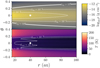 |
Fig. 1 Initial conditions for density (above) and temperature (below), obtained using the iterative procedure described in Sect. 2.3. White lines indicate the corresponding cooling-time contours, computed using Eq. (8). Due to our constant dust-to-gas ratio and assumption of small dust grains throughout the disk, we obtain shorter radiative–diffusion and gas–grain coupling times than in Bae et al. (2021). |
2.3 Setup and initial conditions
In all simulations presented here, we assumed a disk gas surface density profile of
 (11)
(11)
which corresponds to an Md = 0.012 M⊙ within our domain. As in our previous works (e.g., Melon Fuksman & Klahr 2022; Melon Fuksman et al. 2024a,b), we approximated the behavior of the gas with an ideal equation of state, with adiabatic index γ = 1.41 and mean molecular weight µ = 2.32 The total dust-to-gas ratio was assumed to be 1%, of which we took 10% by mass (corresponding to fd = 10−3) to be the small grains that we modeled. These consist of 62.5% silicate and 37.5% graphite, with a material density ρgr = 2.5 g cm−3 and a specific heat capacity cd = 0.7 Jg−1 K−1 ; their sizes follow an MRN (Mathis et al. 1977) distribution, n(a) ∝ a−3.5, with amin = 5 nm and amax = 250 nm. Using the frequency-dependent opacities given by Krieger & Wolf (2020, 2022), we created tables of Planck and Rosseland opacity for this grain distribution as a function of temperature.
To obtain initial conditions, we employed the same iterative technique used in Melon Fuksman & Klahr (2022), cycling hydrostatic-equilibrium and radiative transfer calculations on a timescale (titer = 0.1 y) much shorter than thermal diffusion times through the disk. We ran 1000 iterations in order to obtain a well-converged background profile and used this profile as the initial condition for all simulations, regardless of the physics prescription implemented.
For our planet, located at rp = 40 au, θp = π/2, and ϕρ = π/4, this profile yields a local temperature Tp = Tg.0(r = 40au,θ = π/2) = 26 K and a scale-height ratio (H/r)p = 0.065. We plot our initial conditions in Fig. 1, along with contours for the gas-grain coupling time (on the upper density plot) and radiative cooling time (on the lower temperature plot), normalized by the local dynamical time to obtain effective /β-values; in our β cooling simulations we simply added βdg + βrad. Compared with the detailed calculations of Bae et al. (2021), who self-consistently computed grain settling, opacities, and radiative cooling rates, our assumption of globally constant dust-to-gas ratio and grain size distribution yields shorter cooling times throughout the disk. In the upper atmosphere, this is because our unsettled small grain distribution makes collisional coupling more efficient; in the midplane, the low opacities of these small grains at tens of Kelvin shortens the thermal diffusion timescale.
For all simulations presented here, we used WENO3 reconstruction, along with a van Leer limiter and shock flattening to ensure stability. Our grid resolution was 268(r) × 116(θ) × 919(ϕ), logarithmically spaced in the radial and evenly spaced in the polar and azimuthal. Our domain extended between r = {0.4,2.5} × rp, θ = {−0.4,0.4} + π/2, and ϕ = {0,2π}. Given these dimensions, our resolution yields ~10 cells per scale height at the planet location, the same amount used in historical 2D and 3D simulations of planetary gap-opening (Fung et al. 2014; Fung & Chiang 2016), and higher than in the 3D spiral simulations of Muley et al. (2021), but somewhat lower than in the 2D simulations of Ziampras et al. (2023), which contains a more detailed analysis of the angular-momentum fluxes and multi-gap opening induced by spirals. We used a reduced speed of light ĉ = 10−4c, which Muley et al. (2023) found to work well for analogous simulations of spirals driven by planets tens of au from their host stars.
In the 2T case, our test simulations show that disk columns can oscillate around the midplane, with low-order azimuthal modes undergoing linear growth. Because these modes do not manifest in the isothermal and β cooling simulations, and appear even in the absence of a planet, we tentatively attribute them to some form of irradiation (Fung & Artymowicz 2014) or self-shadowing (e.g., Melon Fuksman & Klahr 2022, and references therein) instability. In the 3T case, this effect is naturally suppressed – we surmise due to the decoupling between gas and dust temperatures at the high altitudes where stellar irradiation is intercepted. As such, for the 2T simulation only, we imposed rapid wave-damping zones in the upper and lower regions of the domain where |θ − π/2| > 0.3, and defer further investigation of this phenomenon to future work.
3 Disk physics
3.1 Thermodynamic prescriptions
In Fig. 2, we plot perturbations in density (ρ), gas temperature (Tg), dust temperature (Td), and perturbations in radial (in center-of-mass coordinates) velocity (υr) for each of our four thermodynamic prescriptions (to recapitulate, local isothermal-ity, β cooling, 2T radiation hydrodynamics, and 3T radiation hydrodynamics). We took cuts of these variables at r = 1 . 5rp at θ = 0 and θ = 0.2 above the midplane, at t = 2500 yr3.
In the midplane, we find that perturbations in ρ and υr are closely aligned with one another in ϕ. In agreement with previous results (e.g., Zhu et al. 2015; Muley et al. 2021), we find these perturbations strongest in the locally isothermal simulations. Among our non-isothermal runs, perturbations in ρ, υr, and Tg are similar regardless of whether a β cooling, 2T, or 3T prescription is used. Tg perturbations capture the work done by compression and expansion (pdV) on a fluid parcel in the disk over one thermal relaxation time. In the midplane of our fiducial disk, this is typically comparable to or shorter than the spiral-crossing time (β ≲ 1), so the measured Tg is relatively weak and somewhat offset in ϕ with respect to the ρ perturbation (which traces the integrated compression and expansion over a fluid parcel’s orbit).
Owing to the very short dust-gas coupling time tc in this region, Td closely follows Tg, and likewise agrees between the 2T and 3T setups. The β cooling simulation, which assumes a constant background temperature, is inherently unable to capture changes in Td. Unlike in the 2D FLD simulations of Ziampras et al. (2023), we do not observe substantial radiative heating of the pre-shock region by emission from hot, post-shock gas (e.g., Ensman 1994). This may be caused by efficient cooling through the disk surface (Ziampras 2023, priv. comm.) in our relatively low-mass, optically thin disk.
This picture becomes somewhat more complicated at θ = 0.2, where the cooling time lengthens, and becomes dominated by dust-gas decoupling rather than radiative diffusion. The ρ spiral is sharp in the locally isothermal case, but weaker in the other simulations. Td agrees between the 2T and 3T simulations, but the gas temperature differs, indicating that observational signatures observable in the upper disk gas (in, e.g.,12CO) may not be reflected in the dust.
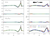 |
Fig. 2 Relative differences in disk density, dust temperature, gas temperature, and radial velocity at t = 2500 yr ≈ 10 orbits with respect to initial conditions for different physical prescriptions. We take azimuthal cuts over the whole 2π at fixed r = 1.5rp and θ = 0 (left) and 0.2 (right) above the midplane. Dust temperatures largely agree between the 2T and 3T cases, whereas gas temperatures largely agree between the 3T and β cooling cases. |
3.2 Lindblad and buoyancy resonances
The observed disk signatures are, in large part, driven by resonant interactions between the disk and the planet’s gravitational potential. One such interaction, studied by decades of analytical and numerical work, occurs at the “Lindblad resonances,” where the Doppler-shifted planetary forcing frequency times an azimuthal integer wavenumber m equals the epicyclic frequency κ (e.g., Goldreich & Tremaine 1978, 1979, 1980; Kley & Nelson 2012; Bae & Zhu 2018a,b). Assuming that the disk is thin, and that the spirals are tightly wound (kr ⪢ mr−1 ) so the Wentzel-Kramers-Brillouin (WKB) approximation holds, we obtain the following dispersion relation:
 (12)
(12)
where Ωp is the planet’s orbital frequency, and kr is the radial wavenumber of the excitation. Given that in a Keplerian disk κ = Ω ∝ r−3/2, we can rewrite the above in terms of kr and m, and integrate to find the phase of the mth spiral mode:
![${\phi _{L,m}}(r) = \int_{{r_{\rm{m}}}}^r {{{\left[ {{{H\left( {{r^\prime }} \right)} \over {{r^\prime }}}} \right]}^{ - 1}}} {\left[ {{{\left( {1 - {{{\Omega _{\rm{p}}}} \over {\Omega \left( {{r^\prime }} \right)}}} \right)}^2} - {m^{ - 2}}} \right]^{1/2}}{\rm{d}}{r^\prime }$](/articles/aa/full_html/2024/07/aa49739-24/aa49739-24-eq31.png) (13)
(13)
where rm = (1 + m−1)2/3 rp is the resonance location. A more detailed analysis, going beyond the WKB approximation (Artymowicz 1993; Papaloizou et al. 2007) shows that the peak mode strength occurs at approximately m ≳ 2/(H/r), above which wave excitation becomes inefficient.
One can also perform a similar analysis on the buoyancy resonances, where the m-multiplied, Doppler-shifted forcing frequency equals the (vertical) Brunt-Väisälä frequency
Nɀ = 𝑔γ−1 [ln P/ργ]1/2 (Lubow & Zhu 2014). These are an inherently 3D phenomenon, depending sensitively on the disk’s thermal physics prescription. Applying the thin-disk approximation that vertical gravity 𝑔 ≈ Ω2ɀ and assuming a background in hydrostatic equilibrium, one can simplify the above to
![${m^2}{\left( {\Omega - {\Omega _{\rm{p}}}} \right)^2} = N_z^2 = {\Omega ^2}z\left[ {{1 \over {{T_{{\rm{g}},0}}}}{{{\rm{d}}{T_{{\rm{g}},0}}} \over {{\rm{d}}z}} + {{\gamma - 1} \over \gamma }{{{\Omega ^2}z} \over {c_{{\rm{s}},{\rm{iso}},0}^2}}} \right],$](/articles/aa/full_html/2024/07/aa49739-24/aa49739-24-eq32.png) (14)
(14)
where  is the isothermal sound speed in the initial condition. Following (Zhu et al. 2015; Bae et al. 2021), this can be used to obtain a phase angle for the spiral:
![${\phi _{{\rm{B}},{\rm{m}}}} = \pm 2\pi m\left( {1 - {\Omega _{\rm{p}}}/\Omega } \right){\left[ {{z \over {{T_{{\rm{g}},0}}}}{{{\rm{d}}{T_{{\rm{g}},0}}} \over {{\rm{d}}z}} + {{\gamma - 1} \over \gamma }{{{\Omega ^2}{z^2}} \over {c_{{\rm{s}},{\rm{iso}},0}^2}}} \right]^{ - 1/2}}.$](/articles/aa/full_html/2024/07/aa49739-24/aa49739-24-eq34.png) (15)
(15)
In Fig. 3, we plot the phase angles for our 3T simulations, density for Lindblad spirals and meridional velocities for buoyancy spirals. Lindblad spirals are clearly visible at all altitudes, but are somewhat less tightly bound than the linear WKB theory of Eq. (13) would predict, given the fiducial planet’s “thermal mass”  of 1.12. The deviation becomes stronger, and the spiral arm becomes more open, with increasing altitude (an effect also seen in the locally isothermal, temperature-stratified simulations of Juhász & Rosotti 2018). The vertical velocity component of the Lindblad spirals also becomes more pronounced in the disk upper atmosphere, especially in the inner disk where scale height is lower than at the wave-launching location near the planet.
As expected, buoyancy spirals are only visible in the upper layers of the disk, but likewise deviate somewhat from the linear phase prediction from Eq. (15). In comparison to previous works, the fact that the thermal relaxation time  , even at high altitudes, acts to damp the buoyant oscillations. We surmise that they could be strengthened through substantial dust growth, settling, or depletion, which would increase the gas–grain coupling time, tc, or alternatively (especially at θ ≈ 0.1 from the midplane, and in the inner disk) by a high dust-to-gas ratio or disk mass, which would increase the thermal diffusion time tdiff.
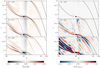 |
Fig. 3 Density, with the planetary spirals indicated (left), and meridional velocity (right) for various altitudes in the disk. Phase predictions for the primary Lindblad arm (Eq. (13), thick line) and m = 3 buoyancy arm (Eq. (15), thin line) are overplotted. In all panels, the cylindrical radius, R = r sin θ, is plotted on the x-axis and the azimuthal angle, θ, on the y-axis. Due to the relatively rapid thermal relaxation in this simulation, buoyancy spirals are markedly weaker than Lindblad spirals in all cases. |
3.3 Flow analysis
We next turned our attention to the flow patterns in the disk. In Figs. 4–6, we plot streamlines of the fluid flow in various disk cuts, along with quivers indicating the instantaneous flow direction (see the captions for more details); in the background, we include the density perturbation for reference. Close to the mid-plane, velocities are essentially restricted to the r –ϕ direction as in 2D simulations; however, at the temperature transition, the spiral pattern weakens and bends, with the velocity acquiring a θ-component (see also, e.g., Boley & Durisen 2006, for a more general discussion of vertical spiral velocities).
What gives rise to these flow patterns, and in turn, how do they influence the observed spiral perturbations in density, temperature, and kinematics? Our system is initialized in a background state ρ0, Tg,0, υ0, where  is a divergence-less, axisymmetric, quasi-Keplerian flow set by the stellar potential Φ* and the initial pressure profile P0. All quantities (ρ, Tg, Td, υr, υθ, and υϕ) can be expressed in terms of the initial condition and a perturbation, for example ρ = ρ0 + ρ′; both the initial condition and perturbation are, in general, dependent on space Working in the rotating frame of the planet, and given that we do not include gas opacities, we can write the evolution of the perturbations as follows:
![${{\partial {\rho ^\prime }} \over {\partial t}} = - \left[ {\upsilon \cdot \nabla {\rho ^\prime } - {\upsilon ^\prime } \cdot \nabla {\rho _0}} \right] - \left[ {\rho \nabla \cdot {\upsilon ^\prime }} \right]$](/articles/aa/full_html/2024/07/aa49739-24/aa49739-24-eq38.png) (16a)
(16a)
![${{\partial T_{\rm{g}}^\prime } \over {\partial t}} = - \left[ {\upsilon \cdot \nabla T_{\rm{g}}^\prime + {\upsilon ^\prime } \cdot \nabla {T_{{\rm{g}},0}}} \right] - (\gamma - 1)\left[ {{T_{\rm{g}}}\nabla \cdot {\upsilon ^\prime }} \right] - t_{\rm{c}}^{ - 1}\left[ {T_{\rm{g}}^\prime - T_{\rm{d}}^\prime } \right]$](/articles/aa/full_html/2024/07/aa49739-24/aa49739-24-eq39.png) (16b)
(16b)
![${{\partial {\upsilon ^\prime }} \over {\partial t}} = - \left[ {\upsilon \cdot \nabla {\upsilon ^\prime } - {\upsilon ^\prime } \cdot \nabla {\upsilon _0}} \right] - \left[ {\nabla P/\rho - \nabla {P_0}/{\rho _0} + \nabla {\Phi _{\rm{P}}}} \right] - 2{{\bf{\Omega }}_{\rm{p}}} \times {\upsilon ^\prime }.$](/articles/aa/full_html/2024/07/aa49739-24/aa49739-24-eq40.png) (16c)
(16c)
In these equations, the partial time-derivative terms represent overall evolution of the quantity at a fixed location; given that the spiral is well developed at t = 2500 yr, and that its pattern speed equals the frame rotation speed, the system is approximately in steady state and these terms net to a small number. The terms in the first set of square brackets, including velocities projected along gradients of various quantities, represent advec-tion of the flow. We considered both the vertical (formally, along the  direction) and in-plane (formally, along the
  and
and  directions) transport of perturbed density, temperature, and velocity within our stratified disk; we write explicit expressions for these terms in Appendix B.
In the second set of square brackets are source terms representing gas compressibility, pdV work, and pressure-gravity balance in Eqs. (16a), (16b), and (16c), respectively. For simplicity, we aggregated the last of these quantities into
![${\left( {{{\partial {\upsilon ^\prime }} \over {\partial t}}} \right)_{{\rm{source }}}} = - \left[ {\nabla p/\rho - \nabla {p_0}/{\rho _0} + \nabla {\Phi _{\rm{p}}}} \right]{\rm{. }}$](/articles/aa/full_html/2024/07/aa49739-24/aa49739-24-eq44.png) (17)
(17)
The final bracketed term in Eq. (16b) represents the exchange of energy between gas and dust. The term 2ΩP × υ′ in Eq. (16c) is the Coriolis acceleration arising from frame rotation. In the second set of square brackets are the source terms, involving divergences of velocities for the scalar quantities, and gradients of pressure/gravitational potential for the velocity.
We plot all of these terms and vertical-advective terms in a cut at r = 1.5rp and θ = 0.2 in Fig. 7. As fluid in this upper-disk region enters the spiral density wave, its quasi-Keplerian orbit is perturbed downward (due to a change in the pressure-gravity balance, υθ) toward the midplane – against ∇ρ0, but along ∇Tg,0 – decreasing the local Tg while increasing ρ (θ advection). Because this flow pattern (which also includes a perturbation in υr) has a nonzero divergence, it also increases ρ and Tg via compression and pdV work, respectively. These terms are balanced by quasi-Keplerian transport of gas through the spiral pattern (“in-plane” advection), and additionally for Tg, colli-sional relaxation to the background dust temperature (cooling), which hold the system in an approximately steady state.
For velocity, vertical gradients are much weaker, so the θ velocity does not play a significant role. Instead, perturbations in the υr and υθ components are governed primarily by the planet-driven density wave (pressure-gravity) and counterbalanced by in-plane transport across the spiral. Along the ϕ-component, the pressure gradient is weak, and υϕ is governed instead by a balance between in-plane advection and Coriolis terms. The fact that υr and υphi are somewhat out of balance reflects the fact that over the long term, planet-driven spirals open a gap in the disk.
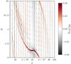 |
Fig. 4 Midplane flow pattern in our disk, in the corotating frame of the planet. Streamlines proceed from bottom to top inside the planet radius rp = 40 au, and from top to bottom outside the planet radius. |
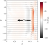 |
Fig. 5 Flow pattern at r = 1.5rp = 60au in an azimuthal cut of the disk. Streamlines flow from right to left; unlike in Fig. 4, vector arrows represent velocity differences from the local initial (quasi-)Keplerian value, rather than from the planet’s Keplerian speed. |
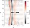 |
Fig. 6 Flow pattern at r = 0.66rp = 26.6au in an azimuthal cut of the disk. Streamlines flow from left to right; as in Fig. 5, vector arrows represent velocity differences from the local initial (quasi-)Keplerian value. |
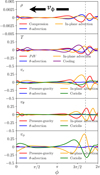 |
Fig. 7 Source (red) and advective (blue) terms at a fixed r = 1.5rp and θ = 0.2, plotted over azimuthal angle ϕ. From top to bottom, we plot these terms for ρ (in units of Ωpρ0,p), Tg (ΩpTg,0,p), υr, υθ, and υϕ (Ωpcs,iso,p), where the p subscript indicates quantities taken at the planet location in the initial condition. A thin dashed gray line passes through the azimuthal peak of the density spiral, showing the significant offset between terms driving spiral perturbations in each quantity. |
3.4 Equilibrium temperature
Disk-planet interaction not only heats the disk locally through pdV work, but non-locally by changing the background radiation field. Spiral arms, for instance, push disk material to higher altitudes, intercepting direct stellar irradiation while gently shadowing the regions behind them. Closer to the midplane, the accumulation of material in circumplanetary regions leads to clearer, radially directed shadowing . The gas heating in both regions, whether through spiral compression or gas accretion, also makes them weak4 sources of radiation. All this impacts the equilibrium temperature Teq, defined by the equation
 (18)
(18)
which incorporates both stellar irradiation and the thermalized radiation field, and whose solution we found using Newton-Raphson iterations. Because these effects depend on the (inherently non-local) transport of radiation, they cannot be accounted for using a β cooling approach; conversely, the deviation of Td,eq from the initial condition Td,0 provides a good measure of the suitability of a β cooling prescription for a particular problem.
In Fig. 8, we plot deviations of Teq, Td, and Tg in our 3T, Saturn-mass simulation; we fixed r = 1.5rp and θ = {0,0.1,0.2}, and plotted the deviations as a function of azimuthal angle. We find that deviations in equilibrium temperature are strongest at ϕ ≈ π/4, the angular position of the planet, resulting from mid-plane shadowing and upper-atmosphere exposure to radiation. This corresponds to the bright “pseudo-arm” observed in Monte Carlo radiative-transfer modeling of near-infrared scattered light from simulated planetary spirals (Muley et al. 2021). The deviations in Teq located approximately π/4 rad from the spiral arms are much weaker; given that they are not centered on the gas temperature bump, we attribute them to rearrangement of disk density affecting transport of stellar and reprocessed radiation, rather than emission from the spiral itself found by Ziampras et al. (2023).
As in Muley et al. (2023), we find that dust and gas temperatures largely agree with each other at lower disk layers, whereas in the upper atmosphere, longer dust-gas coupling mean that the gas temperature reflects pdV work from the spirals, while the dust temperature closely tracks the equilibrium temperature. The generally small deviation of Teq explains why the β cooling approach discussed in Sect. 2.1.3 provides generally accurate results for non-accreting, Saturn-mass planets. However, for other setups – such as those we discuss in the following sections – this need not be the case, and radiation hydrodynamics are essential to obtaining physically consistent results.
4 Parameter study
We tested three different planet masses (Mp = {5 × 10⁻⁵, 3 × 10⁻⁴, 1 × 10⁻³ M⊙, corresponding to Neptune-, Saturn-, and Jupiter-mass, respectively)5 with no accretion luminosity, and two planetary accretion luminosities (Lacc,p = {0,1 × 10⁻³}) with a Saturn-mass planet. In order to capture changes to the background radiation field – which become especially pronounced for high-mass or accreting protoplanets – we used the full 3T scheme for all of these simulations.
4.1 Planet mass
In Fig. 9, we plot the spiral-averaged perturbation amplitude  – where x can be any one of various normalized quantities (lnρ/ρ0, ln Tg/Tg,0, ln Td/Td,0, υr/cs,iso,p, υθ/cs,iSo,p, υϕ/ cS,iso,p), and ∆x its deviation from the initial condition – as a function of planet mass. As in previous figures, we fixed r = 1.5rp and tested θ = {0.0,0.1,0.2} above the midplane. We defined
 (19)
(19)
which is analogous to the definition in Muley et al. (2021), with the important distinction that in the present work the amplitude is not vertically averaged. Open circles indicate simulations without accretion luminosity, while filled circles correspond to our simulation with it (Sect. 4.2).
As found in previous works (Fung & Dong 2015; Dong & Fung 2017; Muley et al. 2021), spiral amplitude increases substantially with planet mass, irrespective of the measure used. At θ = 0.0 and θ = 0.1, ρ and υr/cS,iSo,p perturbations follow each other closely; both weaken in the upper atmosphere, but the density perturbation much more so. υθ/cs,iso,p is nearly zero in the disk midplane, but rises with increasing altitude (see Sect. 3.3). υϕ/cS,iso,p is relatively weak in most cases, but is stronger for high-mass cases at θ = 0.1,0.2 thanks to the distortions introduced by the circumplanetary flow. At every altitude and planet mass, temperature deviations tend to be weaker than those in density and velocity. At θ = 0.0,0.1 where dust and gas are well coupled, they reflect both the Lindblad spiral and the radial pseudo-arm instead (Sect. 3.4), but at θ = 0.2, gas temperature primarily reflects the Lindblad spiral while dust temperature reflects the pseudo-arm.
For a more qualitative understanding, we show 2D polar cuts of υr in Fig. 10. Sub-thermal, Neptune-mass planets excite well-behaved kinematic spirals that are clearly distinct from the laminar background; however, these spirals are rather weak, with typical |υr| ≲ 0.1cS,iso,p – corresponding to a physical velocity of ≲30m s−1 in our disk model. In the Saturn-mass case, velocity spirals have a similar shape, but are significantly stronger – by a factor of ~4 in the outer disk (Fig. 9), and even more so in the inner disk. Here, flows at the corotation radius and in the vicinity of the planet, which can be identified with the velocity kinks observed in channel maps (e.g., Pinte et al. 2019), become significantly more prominent.
In the Jupiter-mass case, Lindblad spirals become somewhat stronger, with higher-order spirals (Bae & Zhu 2018a,b) particularly visible in the inner and upper disks. However, the observed υr signature is dominated by flows near the planet, which become larger and faster thanks to the greater planet mass and gravitational sphere of influence. In the upper atmosphere, this flow takes on a wing-like shape, and acts to bring material directly above/below the planet, where is funneled toward the planet’s Hill radius through the poles (e.g., Fung et al. 2015, 2019). At all altitudes, the background flow also becomes unsteady and more turbulent.
To complement our understanding from the kinematic signatures, we present perturbations in the gas temperature Tg in Sect. 3.4, taken at the same 2D polar cuts as in Fig. 10. In all simulations, we observe a radial shadow from the circumplane-tary region (see Sect. 3.4) whose strength increases with the size of the circumplanetary region and thus, with planet mass. Especially for higher-mass cases, the fact that the integrated one-sided Lindblad torque scales as  (Tsang 2011) may contribute to strengthening the outer spiral. In the upper atmosphere, the funneling of gas into a flow toward the midplane along the planetary pole leads to compressional heating, manifesting as a hot spot in Tg above the planet location.
Thermal relaxation, first by gas–grain collision and then by thermal emission from heated dust grains, dissipates pdV work to the radiation field. For the disk setup we chose, the effective relaxation timescale (β = 0.1−1) is approximately equal to or less than the spiral crossing time. As a result, the Tg spiral has a multiband structure, reflecting the initial compression when the gas strikes the spiral (high-temperature band), expands behind the spiral (low-temperature band), and compresses again to return to the background density (high-temperature band). The first high-temperature band is dominant in the midplane, but both roughly even in the disk upper atmosphere. This stands in contrast to the effectively adiabatic situation where thermal relaxation is much slower than spiral crossing (Miranda & Rafikov 2020b; Muley et al. 2021), where the Tg spiral reflects the accumulated total of compression and expansion rather than individual short phases of it. This picture is clear up to Saturn-mass, but less so at Jupiter-mass, where the Tg Lindblad spiral is distorted by the effects of circumplanetary and turbulent flows.
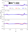 |
Fig. 8 Background equilibrium, gas, and dust temperatures in our 3T, Saturn-mass simulations at selected altitudes above the midplane for a fixed r = 1.5rp. Background temperatures deviate by only a few percent from the initial condition, most strongly in the region of the planetary shadow (ϕ ≈ π/4) and somewhat more weakly near the Lindblad spiral. Td agrees well with Tg at θ = 0.0 and 0.1 (and is covered by the line for Tg), and with Teq at θ = 0.2 (covering the line for Teq). |
4.2 Accretion luminosity
In recent years, the effect of planetary accretion luminosity has been studied in parametrized 2D global disk simulations (Montesinos et al. 2015, 2021; Gárate et al. 2021), and in local, 3D simulations with full radiative transfer (Szulágyi 2017) that emphasize the circumplanetary disk. We add to this body of work with our 3D global simulations, including 3T radiation transport and a luminous planet. The Lacc,p = 10−3L⊙ we used corresponds to a mass accretion rate of  , given the fiducial planet mass Mp = 4 × 10⁻⁴ M⊙ and assuming a typical radius of 2 RJ for the forming planet. For this mass, such an accretion rate can only be sustained over brief periods. We thus believe that this scenario, along with the no-accretion base-case, bracket the range of accretion luminosities that the planet might experience during its growth.
We revisit Fig. 9, in which spiral amplitudes from our simulations with accretion luminosity are plotted with filled circles. At r = 1.5rp and θ = 0, accretion luminosity somewhat weakens the ρ and υr perturbations, while leaving the others unchanged. At higher altitudes, by contrast, most perturbations are significantly strengthened by accretion luminosity – sometimes by factors of 2 or more – with respect to the nonluminous planet case.
Along the lines of Figs. 10 and 11, we also made qualitative plots of kinematic and temperature perturbations at various disk cuts, and present these in Fig. 12. With planetary accretion luminosity, the circumplanetary envelope becomes more pressure-supported, with the hot core overflowing the planetary Hill radius. Close to the midplane, this disrupts the orderly Doppler-flip kinematic signature and enhances the Lindblad spirals in both temperature and velocity, without changing their overall morphology. It also significantly strengthens the outer radial shadow (Montesinos et al. 2021) through its impact on the envelope’s vertical and azimuthal structure.
In the upper atmosphere, however, accretion luminosity intensifies the spiral and changes its shape. The radial velocity shows a double-banded structure – as opposed to the single-banded one expected without accretion luminosity – while the temperature shows a cold-hot-cold band structure, rather than hot-cold-hot. With accretion, the spiral also remains strong much farther away from the planet than without.
To understand these results better, we plot the density perturbation in Fig. 13, at a vertical cut through the planet’s azimuth at ϕp, = π/4. In this view, it is clear that accretion luminosity puffs the circumplanetary region vertically. This changes the flow pattern significantly, with accretion primarily happening by material diagonally striking the edge of the envelope, rather than being funneled downward into a narrow polar flow perpendicular to the disk midplane, as is classically the picture (e.g., Fung et al. 2015). This is responsible for many of the observed changes to kinematic and thermal signatures, particularly in the upper atmosphere. Moreover, this means that material flowing into the Hill sphere has higher angular momentum in the accreting than non-accreting case and, as such, preferably gets expelled outward.
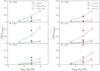 |
Fig. 9 Measurement of the azimuthal perturbation in each normalized quantity x, averaged over an azimuthal range of ϕpeak ± 2hp according to Eq. (19). Densities and temperatures are plotted in the left panel and velocities in the right. Open circles indicate non-accreting planets, and closed circles indicate those with accretion luminosity (see Sect. 4.2 for a discussion). At z/r ≈ θ = 0.2, where dust and gas are not well coupled, the plotted Tdust amplitude reflects the radial “pseudo-arm” (see the discussion in Sect. 3.4) rather than the Lindblad spiral. |
5 Observational implications
Of the cases we tested, we find that (non-accreting) Saturn-mass planets, accreting Saturn-mass planets, and Jupiter-mass (non-accreting) planets are best at driving thermal and kinematic signatures that are amenable to observation. In each of these cases, we plot the planet-induced total velocity perturbation – projected along the line of sight ( ) – in Figs. A.1, A.2, and A.3, respectively. In Figs. A.4, A.5, and A.6, we likewise plot the perturbations in gas temperature Tg. In these figures, we take a cut at θ = 0.3 above the midplane; this corresponds to ~4.6 scale heights at rp, and roughly aligns with the expected 12CO J = (2−1) emission layer (Barraza-Alfaro et al. 2024). (The θ = 0.2 surface shown prominently in previous figures, at ~3.1 scale heights above the midplane, is closer to the 12CO J = (3−2) layer.) We tested disk inclinations id = {0°, 30°, 60°} and planetary position angles ϕp = {0°, 90°, 180°, 270°}.
For an  , is dominated by
  . In the non-accreting, Saturn-mass fiducial case, the observed velocity spiral is driven by the local pressure-gradient term, as identified in Sect. 3.3; the redshifted spot above the planet location reflects the polar planetary flow shown in Fig. 13. For the Saturn-mass planet with accretion luminosity, the outer Lindblad spiral is noticeably stronger and extends over a greater distance, while the planetary flow – no longer oriented in a polar direction – aligns with it, forming a double-banded velocity profile as discussed in Sect. 2.2. In the Jupiter-mass case, the polar accretion flow is more prominent than in the fiducial case, with the spiral becoming subdominant. In observations, these features could help distinguish between prominent spirals created by high-mass planets and those created by highly luminous ones.
As disk inclination increases from zero,  increasingly reflects
  (and to a lesser extent
  ). Because the typical magnitude of
  in spirals is typically much larger than
  , this strengthens the observed spiral signature, both in the inner and outer disks. Inclination also interacts with the elevation angle θ = 0.3 of the plotted disk surface to distort the sky-projected areas of surface elements in an azimuthally dependent way, with disk patches on the near side of the star appearing smaller than those on the far side. Depending on the planetary position angle,ϕp these properties can emphasize or deemphasize the circumplanetary region, inner, or outer spirals.
In each case, temperature spirals generally follow the same structure as the kinematic spirals; however, the magnitude of the observed temperature perturbation at a given point in the disk is a scalar quantity, and unlike  does not change with projection. Furthermore, as discussed in Sects. 3.1 and 4.1, the nonzero, finite cooling time introduces a slight offset between the temperature and velocity perturbations. Conversely, the offset between kinematic and thermal spirals – as well as the prominence of buoyancy spirals – in different tracers probing various disk layers (e.g., as studied in the MAPS program; Calahan et al. 2021) could help put limits on cooling time at various vertical positions in the disk. Planet-induced radial midplane shadows could also be used to measure cooling rates – by measuring their deviation from a straight line going through planet and star – provided that the planet’s position angle is well constrained. However, fully exploring these mechanisms would require a large hydrodynam-ical parameter that covers a range of disk masses and dust size distributions.
Our simulations were run for a relatively short period of time, emphasizing the development of spiral density waves. This means that the effects of gap opening - in particular, changes to disk illumination and equilibrium temperature (Jang-Condell & Turner 2012) and changes to  due to the pressure gradient at gap edges (Armitage 2020, Sect. 2.4) – have not had the time to fully develop. Especially in the Jupiter-mass case, these effects can be substantial. Simulations to gap-opening timescales are currently in progress, and we intend to present them – along with Monte Carlo radiative-transfer post-processing and synthetic observations – in a forthcoming work.
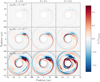 |
Fig. 10 Radial velocities, υr, from 3T, zero-accretion-luminosity simulations with Neptune-mass (top row), Saturn-mass (middle row), and Jupiter-mass (bottom row) planets, at various altitudes in the disk (left, middle, and right columns). Gray circles indicate the planetary Hill radius. All υr values are expressed as a function of initial isothermal sound speed at the location of the planet, |

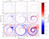 |
Fig. 11 Gas temperature perturbation for Neptune-mass (top row), Saturn-mass (middle row), and Jupiter-mass (bottom row) planets, at various altitudes in the disk (left, middle, and right columns). Gray circles indicate the planetary Hill radius. All temperature values are expressed with respect to the initial condition Tg,0. |
6 Conclusion
We have run 3D, 3T radiation hydrodynamical simulations with the aim of better understanding the kinematic signatures that would be generated by forming protoplanets. Our fiducial setup, with a non-accreting Saturn-mass planet located at rp = 40au in a 15 MJ disk, draws inspiration from the TW Hya system, where spiral arms – potentially excited by a forming planet (e.g., Muley et al. 2021; Bae et al. 2021) – have already been observed via temperature and velocity measurements (e.g., Teague et al. 2019). First, we studied the physical properties of the simulated planet-driven spirals and compared our 3T approach to several thermodynamic prescriptions commonly used in the literature. Thereafter, we investigated the effects that changing planetary masses and accretion luminosities have on the strength and morphology of planet-driven disk features.
For our fiducial disk, we find that the results of our 3T simulations agree well with those from physically motivated β cooling. This naturally follows from the fact that for this setup the background equilibrium temperature, Teq, does not change much from the initial condition. As expected from previous works (e.g., Juhász & Rosotti 2018; Muley et al. 2021; Bae et al. 2021), Lindblad spirals become more open with higher altitudes in the stratified temperature background; buoyancy spirals are weak in strength due to the relatively short cooling times we used. In the upper disk – most amenable to observation in 12CO – thermal and kinematic signatures are driven largely by local source terms, rather than transport across vertical gradients within the disk.
Our parameter survey shows that thermal and kinematic Lindblad spirals become stronger at high planet masses. Especially in the super-thermal mass regime, deeper planetary potential wells and larger Hill radii also enhance the signatures of circumplanetary flows. Planetary accretion luminosity adds pressure support to the circumplanetary region and reorients the classic polar accretion flows (e.g., Fung et al. 2015, 2019; Fung & Chiang 2016) slightly outward. The separate effects of increasing planet masses and accretion luminosities, relative to our fiducial case, are clearly visible in our sky-projected, inclined, and rotated plots of the upper disk layers and, thus, potentially in ALMA line observations.
Future areas of research could include testing different disk masses and dust-to-gas ratios, increasing resolution to allow for the development of hydrodynamical instabilities, which may impact the visibility of spiral signatures (e.g., Barraza-Alfaro et al. 2024), or running simulations to gap-opening timescales (e.g., Fung et al. 2014; Fung & Chiang 2016) and post-processing the results to compare to observations. The last work is currently in progress.
More sophisticated numerical approaches would expand the scope of these comparisons. To more closely reproduce spiral pitch angles and morphologies in real disks (Miranda & Rafikov 2019), particularly for the 20–200 K temperature range spanned by our simulations, it would significantly help to relax the ideal-gas assumption and compute γ as a function of temperature, as well as hydrogen (para-, ortho-, and atomic), helium, and metal fractions (Boley et al. 2007, 2013; Bitsch et al. 2013a). Incorporating multiple dust species (including momentum exchange and turbulent diffusion) would enable modeling of widened, thickened rings of millimeter grains at planetary gap edges (Bi et al. 2021, 2023), which are visible in the dust continuum. On the other hand, a short-characteristics approach to radiation transport (e.g., Davis et al. 2012), which would allow for beam-crossing between accretion luminosity and reprocessed stellar radiation, could more accurately simulate strengths for radial shadows from luminous planets. Coupling such methods with our 3T scheme, however, is a computationally expensive and technically ambitious undertaking that we defer to future work.
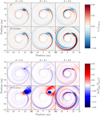 |
Fig. 12 Difference from the initial condition in υr (above) and Tg (below) for 3T simulations of Saturn-mass planets without and with accretion luminosity. The strongly luminous planet alters the vertical and azimuthal structure of the circumplanetary region, causing strong shadows behind the planet and greatly enhancing the kinematic signatures of accretion in the outer disk. |
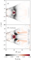 |
Fig. 13 Density perturbation in a cut through ϕρ = π/4 as a function of cylindrical radius, R, and vertical position, ɀ, for 3T simulations of Saturn-mass planets without (above) and with (below) accretion luminosity. Gray arrows indicate the velocity field, and the gray circle encloses the planetary Hill radius. When accretion luminosity is included, the circumplanetary envelope becomes larger and the flow around it is altered. |
Acknowledgements
We thank Myriam Benisty and Kees Dullemond for the suggestion to include sky-projected maps of velocity and temperature, as well as Marcelo Barraza Alfaro and Richard Teague for detailed comments on the manuscript. We also acknowledge useful discussions with Xue-Ning Bai, Jiaqing Bi, Remo Burn, Can Cui, Mario Flock, Gabriel-Dominique Marleau, Dominik Ostertag, Jiahan Shi, Jess Speedie, and Alexandros Ziampras. We thank the anonymous referee for a helpful report, and particularly for encouraging us to comment on the equation of state. Numerical simulations were run on the Cobra and Raven clusters of the Max-Planck-Gesellschaft and the Vera Cluster of the Max-Planck-Institut für Astronomie, both hosted by the Max Planck Computing and Data Facility (MPCDF) in Garching bei München. The research of J.D.M.F. and H.K. is supported by the German Science Foundation (DFG) under the priority program SPP 1992: “Exoplanet Diversity” under contract KL 1469/16-1/2.
Appendix A Sky-projected figures
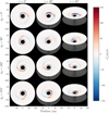 |
Fig. A.1 Sky-projected velocity perturbation, |

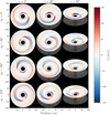 |
Fig. A.2 Sky-projected velocity perturbation, |

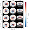 |
Fig. A.3 Sky-projected velocity perturbation, |

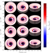 |
Fig. A.4 Perturbation in gas temperature, Tg − Tg,0, at θ = 0.3 above the midplane for our fiducial setup with a Saturn-mass, non-accreting planet. The double-armed structure of the Lindblad spiral in the upper atmosphere is clearly visible here. |
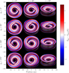 |
Fig. A.5 Gas temperature perturbation for an accreting Saturn-mass planet. As with the kinematic spiral, the thermal spiral extends over a larger radial range and is more prominent than in the non-accreting case. |
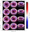 |
Fig. A.6 Gas temperature perturbation for a Jupiter-mass planet. As with kinematics, the circumplanetary region and gap make a much larger contribution to the thermal signature than in the fiducial Saturn-mass, non-accreting case. |
Appendix B Advective terms in spherical coordinates
For a scalar quantity such as density or temperature, the rate of change at a specific location due to advection in any given direction is given by the (negative) gradient of the scalar, projected along the velocity in that direction. The advection of perturbations is given by the advective term in the current state, minus advection in the initial condition.
Making use of the fact that our initial condition is axisym-metric in all variables, and that υr(t = 0) = υθ(t = 0) = 0, we can write the evolution of the density perturbation ρ′ as
 (B.1a)
 (B.1b)
 (B.1c)
and that of the gas temperature perturbation,  , as
, as
 (B.2a)
 (B.2b)
 (B.2c)
For vectors, such as velocity, the advection term includes not only partial derivatives of each component in each coordinate, but also geometric connection terms arising from the change in the basis vectors themselves as a function of coordinate. This yields the following advective terms in each direction:
![${\left. {{{\partial {\upsilon ^\prime }} \over {\partial t}}} \right|_{{\rm{advr}}}} = - \upsilon _{\rm{r}}^\prime \left[ {{\partial _r}\upsilon _{\rm{r}}^\prime \widehat r + {\partial _r}\upsilon _\theta ^\prime \widehat \theta + {\partial _r}{\upsilon _\phi }\widehat \phi } \right]$](/articles/aa/full_html/2024/07/aa49739-24/aa49739-24-eq71.png) (B.3a)
(B.3a)
![${\left. {{{\partial {\upsilon ^\prime }} \over {\partial t}}} \right|_{{\rm{adv}}\theta }} = - {{\upsilon _\theta ^\prime } \over r}\left[ {\left( {{\partial _\theta }\upsilon _{\rm{r}}^\prime - \upsilon _\theta ^\prime } \right)\widehat {\bf{r}} + \left( {{\partial _\theta }\upsilon _\theta ^\prime + \upsilon _r^\prime } \right)\widehat {\bf{\theta }} + \left( {{\partial _\theta }\upsilon _\phi ^\prime + {\partial _\theta }{\upsilon _{0,\phi }}} \right)\widehat \phi } \right]$](/articles/aa/full_html/2024/07/aa49739-24/aa49739-24-eq72.png) (B.3b)
(B.3b)
![$\eqalign{ & {\left. {{{\partial {\upsilon ^\prime }} \over {\partial t}}} \right|_{{\rm{adv}}\phi }} = - {{{\upsilon _\phi }} \over {r\sin \theta }}\left[ {{\partial _\phi }\upsilon _{\rm{r}}^\prime \widehat {\bf{r}} + {\partial _\phi }\upsilon _\theta ^\prime \widehat {\bf{\theta }} + \left( {{\partial _\phi }{\upsilon _\phi } + {\upsilon _{\rm{r}}}\sin \theta + {\upsilon _\theta }\cos \theta } \right)\widehat \phi } \right] \cr & & \,\,\,\, + {{\upsilon _\phi ^2 - \upsilon _{\phi ,0}^2} \over {r\sin \theta }}(\sin \theta \widehat {\bf{r}} + \cos \theta \widehat {\bf{\theta }}) & & & & . \cr} $](/articles/aa/full_html/2024/07/aa49739-24/aa49739-24-eq73.png) (B.3c)
(B.3c)
We emphasize that despite considering only advection in one given coordinate direction, each of the expressions in Equation B.3 has three components, arising from the advection of velocity components orthogonal to the advection direction, as well as the aforementioned geometric connection terms. For ease of interpretation, in Figure 7, we define the in-plane advection as the sum (∂υ′/∂t)adv,in−plane = (∂υ′/∂t)advr + (∂υ′/∂t)advϕ.
References
- Armitage, P. J. 2020, Astrophysics of Planet Formation, 2nd edn Cambridge: (Cambridge University Press) [CrossRef] [Google Scholar]
- Artymowicz, P. 1993, ApJ, 419, 155 [NASA ADS] [CrossRef] [Google Scholar]
- Bae, J., & Zhu, Z. 2018a, ApJ, 859, 118 [Google Scholar]
- Bae, J., & Zhu, Z. 2018b, ApJ, 859, 119 [Google Scholar]
- Bae, J., Teague, R., & Zhu, Z. 2021, ApJ, 912, 56 [NASA ADS] [CrossRef] [Google Scholar]
- Barraza-Alfaro, M., Flock, M., & Henning, T. 2024, A&A, 683, A16 [NASA ADS] [CrossRef] [EDP Sciences] [Google Scholar]
- Bi, J., Lin, M.-K., & Dong, R. 2021, ApJ, 912, 107 [NASA ADS] [CrossRef] [Google Scholar]
- Bi, J., Lin, M.-K., & Dong, R. 2023, ApJ, 942, 80 [NASA ADS] [CrossRef] [Google Scholar]
- Bitsch, B., Boley, A., & Kley, W. 2013a, A&A, 550, A52 [NASA ADS] [CrossRef] [EDP Sciences] [Google Scholar]
- Bitsch, B., Crida, A., Morbidelli, A., Kley, W., & Dobbs-Dixon, I. 2013b, A&A, 549, A124 [NASA ADS] [CrossRef] [EDP Sciences] [Google Scholar]
- Boley, A. C., & Durisen, R. H. 2006, ApJ, 641, 534 [Google Scholar]
- Boley, A. C., Hartquist, T. W., Durisen, R. H., & Michael, S. 2007, ApJ, 656, L89 [NASA ADS] [CrossRef] [Google Scholar]
- Boley, A. C., Morris, M. A., & Desch, S. J. 2013, ApJ, 776, 101 [NASA ADS] [CrossRef] [Google Scholar]
- Bollati, F., Lodato, G., Price, D. J., & Pinte, C. 2021, MNRAS, 504, 5444 [Google Scholar]
- Burke, J. R., & Hollenbach, D. J. 1983, ApJ, 265, 223 [NASA ADS] [CrossRef] [Google Scholar]
- Calahan, J. K., Bergin, E. A., Zhang, K., et al. 2021, ApJS, 257, 17 [NASA ADS] [CrossRef] [Google Scholar]
- Chrenko, O., & Lambrechts, M. 2019, A&A, 626, A109 [NASA ADS] [CrossRef] [EDP Sciences] [Google Scholar]
- Chrenko, O., & Nesvorný, D. 2020, A&A, 642, A219 [NASA ADS] [CrossRef] [EDP Sciences] [Google Scholar]
- Commerçon, B., Audit, E., Chabrier, G., & Chièze, J. P. 2011, A&A, 530, A13 [NASA ADS] [CrossRef] [EDP Sciences] [Google Scholar]
- Davis, S. W., Stone, J. M., & Jiang, Y.-F. 2012, ApJS, 199, 9 [NASA ADS] [CrossRef] [Google Scholar]
- Decampli, W. M., Cameron, A. G. W., Bodenheimer, P., & Black, D. C. 1978, ApJ, 223, 854 [NASA ADS] [CrossRef] [Google Scholar]
- Dong, R., & Fung, J. 2017, ApJ, 835, 38 [Google Scholar]
- Eastwood, J. W. 1986, Comput. Phys. Commun., 43, 89 [NASA ADS] [CrossRef] [Google Scholar]
- Ensman, L. 1994, ApJ, 424, 275 [NASA ADS] [CrossRef] [Google Scholar]
- Fung, J., & Artymowicz, P. 2014, ApJ, 790, 78 [NASA ADS] [CrossRef] [Google Scholar]
- Fung, J., & Chiang, E. 2016, ApJ, 832, 105 [NASA ADS] [CrossRef] [Google Scholar]
- Fung, J., & Dong, R. 2015, ApJ, 815, L21 [NASA ADS] [CrossRef] [Google Scholar]
- Fung, J., Shi, J.-M., & Chiang, E. 2014, ApJ, 782, 88 [NASA ADS] [CrossRef] [Google Scholar]
- Fung, J., Artymowicz, P., & Wu, Y. 2015, ApJ, 811, 101 [Google Scholar]
- Fung, J., Masset, F., Lega, E., & Velasco, D. 2017, AJ, 153, 124 [Google Scholar]
- Fung, J., Zhu, Z., & Chiang, E. 2019, ApJ, 887, 152 [NASA ADS] [CrossRef] [Google Scholar]
- Gárate, M., Cuadra, J., Montesinos, M., & Arévalo, P. 2021, MNRAS, 501, 3113 [CrossRef] [Google Scholar]
- Gnedin, N. Y., & Abel, T. 2001, New A, 6, 437 [NASA ADS] [CrossRef] [Google Scholar]
- Goldreich, P., & Tremaine, S. 1978, ApJ, 222, 850 [NASA ADS] [CrossRef] [Google Scholar]
- Goldreich, P., & Tremaine, S. 1979, ApJ, 233, 857 [Google Scholar]
- Goldreich, P., & Tremaine, S. 1980, ApJ, 241, 425 [Google Scholar]
- Goodman, J., & Rafikov, R. R. 2001, ApJ, 552, 793 [NASA ADS] [CrossRef] [Google Scholar]
- Jang-Condell, H., & Turner, N. J. 2012, ApJ, 749, 153 [NASA ADS] [CrossRef] [Google Scholar]
- Juhász, A., & Rosotti, G. P. 2018, MNRAS, 474, L32 [Google Scholar]
- Klahr, H., & Kley, W. 2006, A&A, 445, 747 [NASA ADS] [CrossRef] [EDP Sciences] [Google Scholar]
- Kley, W. 1989, A&A, 208, 98 [NASA ADS] [Google Scholar]
- Kley, W., & Nelson, R. P. 2012, ARA&A, 50, 211 [Google Scholar]
- Kley, W., Bitsch, B., & Klahr, H. 2009, A&A, 506, 971 [NASA ADS] [CrossRef] [EDP Sciences] [Google Scholar]
- Krieger, A., & Wolf, S. 2020, A&A, 635, A148 [NASA ADS] [CrossRef] [EDP Sciences] [Google Scholar]
- Krieger, A., & Wolf, S. 2022, A&A, 662, A99 [NASA ADS] [CrossRef] [EDP Sciences] [Google Scholar]
- Lega, E., Crida, A., Bitsch, B., & Morbidelli, A. 2014, MNRAS, 440, 683 [Google Scholar]
- Levermore, C. D. 1984, J. Quant. Spec. Radiat. Transf., 31, 149 [NASA ADS] [CrossRef] [Google Scholar]
- Levermore, C. D., & Pomraning, G. C. 1981, ApJ, 248, 321 [NASA ADS] [CrossRef] [Google Scholar]
- Lobo Gomes, A., Klahr, H., Uribe, A. L., Pinilla, P., & Surville, C. 2015, ApJ, 810, 94 [NASA ADS] [CrossRef] [Google Scholar]
- Lubow, S. H., & Zhu, Z. 2014, ApJ, 785, 32 [NASA ADS] [CrossRef] [Google Scholar]
- Mathis, J. S., Rumpl, W., & Nordsieck, K. H. 1977, ApJ, 217, 425 [Google Scholar]
- Melon Fuksman, J. D., & Klahr, H. 2022, ApJ, 936, 16 [NASA ADS] [CrossRef] [Google Scholar]
- Melon Fuksman, J. D., & Mignone, A. 2019, ApJS, 242, 20 [NASA ADS] [CrossRef] [Google Scholar]
- Melon Fuksman, J. D., Klahr, H., Flock, M., & Mignone, A. 2021, ApJ, 906, 78 [NASA ADS] [CrossRef] [Google Scholar]
- Melon Fuksman, J. D., Flock, M., & Klahr, H. 2024a, A&A, 682, A139 [NASA ADS] [CrossRef] [EDP Sciences] [Google Scholar]
- Melon Fuksman, J. D., Flock, M., & Klahr, H. 2024b, A&A, 682, A140 [NASA ADS] [CrossRef] [EDP Sciences] [Google Scholar]
- Mignone, A., Bodo, G., Massaglia, S., et al. 2007, ApJS, 170, 228 [Google Scholar]
- Miranda, R., & Rafikov, R. R. 2019, ApJ, 875, 37 [Google Scholar]
- Miranda, R., & Rafikov, R. R. 2020a, ApJ, 904, 121 [NASA ADS] [CrossRef] [Google Scholar]
- Miranda, R., & Rafikov, R. R. 2020b, ApJ, 892, 65 [NASA ADS] [CrossRef] [Google Scholar]
- Montesinos, M., Cuadra, J., Perez, S., Baruteau, C., & Casassus, S. 2015, ApJ, 806, 253 [NASA ADS] [CrossRef] [Google Scholar]
- Montesinos, M., Cuello, N., Olofsson, J., et al. 2021, ApJ, 910, 31 [CrossRef] [Google Scholar]
- Muley, D., Dong, R., & Fung, J. 2021, AJ, 162, 129 [NASA ADS] [CrossRef] [Google Scholar]
- Muley, D., Melon Fuksman, J. D., & Klahr, H. 2023, A&A, 678, A162 [NASA ADS] [CrossRef] [EDP Sciences] [Google Scholar]
- Papaloizou, J. C. B., Nelson, R. P., Kley, W., Masset, F. S., & Artymowicz, P. 2007, in Protostars and Planets V, eds. B. Reipurth, D. Jewitt, & K. Keil, 655 [Google Scholar]
- Pareschi, L., & Russo, G. 2005, J. Sci. Comput., 25, 129 [MathSciNet] [Google Scholar]
- Pérez, S., Casassus, S., & Benítez-Llambay, P. 2018, MNRAS, 480, L12 [Google Scholar]
- Pinte, C., Price, D. J., Ménard, F., et al. 2018, ApJ, 860, L13 [Google Scholar]
- Pinte, C., van der Plas, G., Ménard, F., et al. 2019, Nat. Astron., 3, 1109 [NASA ADS] [CrossRef] [Google Scholar]
- Pinte, C., Hammond, I., Price, D. J., et al. 2023a, MNRAS, 526, L41 [NASA ADS] [CrossRef] [Google Scholar]
- Pinte, C., Teague, R., Flaherty, K., et al. 2023b, in ASP Conf. Ser., 534, Proto-stars and Planets VII, eds. S. Inutsuka, Y. Aikawa, T. Muto, K. Tomida, & M. Tamura, 645 [NASA ADS] [Google Scholar]
- Skinner, M. A., & Ostriker, E. C. 2013, ApJS, 206, 21 [NASA ADS] [CrossRef] [Google Scholar]
- Speedie, J., Booth, R. A., & Dong, R. 2022, ApJ, 930, 40 [NASA ADS] [CrossRef] [Google Scholar]
- Szulágyi, J. 2017, ApJ, 842, 103 [Google Scholar]
- Teague, R., Bae, J., Huang, J., & Bergin, E. A. 2019, ApJ, 884, L56 [Google Scholar]
- Teague, R., Bae, J., Andrews, S. M., et al. 2022, ApJ, 936, 163 [NASA ADS] [CrossRef] [Google Scholar]
- Tsang, D. 2011, ApJ, 741, 109 [NASA ADS] [CrossRef] [Google Scholar]
- Wölfer, L., Facchini, S., Kurtovic, N. T., et al. 2021, A&A, 648, A19 [NASA ADS] [CrossRef] [EDP Sciences] [Google Scholar]
- Yun, H.-G., Kim, W.-T., Bae, J., & Han, C. 2022, ApJ, 938, 102 [NASA ADS] [CrossRef] [Google Scholar]
- Zhu, Z., Stone, J. M., & Rafikov, R. R. 2012, ApJ, 758, L42 [NASA ADS] [CrossRef] [Google Scholar]
- Zhu, Z., Dong, R., Stone, J. M., & Rafikov, R. R. 2015, ApJ, 813, 88 [Google Scholar]
- Ziampras, A., Kley, W., & Dullemond, C. P. 2020, A&A, 637, A50 [NASA ADS] [CrossRef] [EDP Sciences] [Google Scholar]
- Ziampras, A., Nelson, R. P., & Rafikov, R. R. 2023, MNRAS, 524, 3930 [NASA ADS] [CrossRef] [Google Scholar]
This only strictly holds when the cell spacings in all directions are independent of the corresponding coordinate; in the r direction, where ∆ri; ∝ ri, it is possible for the edge of the kernel to intersect the second cell inward,  . The extent of this edge is, at most,
  , which for our grid is always less than 1% of the kernel half-width; the integral of ψ over this intersecting edge is < O(10−4). We added this small excess to the cells {ip, jp ± 1, kp ± 1}.
We note that within our temperature range of interest (≈20–200 K), γ can vary between 1.3 and 1.66 as rotational modes of the H2 molecule are activated, with the exact index depending on the assumed ortho- and para-hydrogen ratio (equilibrium or some fixed fraction; see e.g., Bitsch et al. 2013a).
The circumplanetary region becomes a much stronger source when accretion luminosity is accounted for; see Sect. 4.2 for more details.
All Figures
|
Fig. 1 Initial conditions for density (above) and temperature (below), obtained using the iterative procedure described in Sect. 2.3. White lines indicate the corresponding cooling-time contours, computed using Eq. (8). Due to our constant dust-to-gas ratio and assumption of small dust grains throughout the disk, we obtain shorter radiative–diffusion and gas–grain coupling times than in Bae et al. (2021). |
| In the text | |
|
Fig. 2 Relative differences in disk density, dust temperature, gas temperature, and radial velocity at t = 2500 yr ≈ 10 orbits with respect to initial conditions for different physical prescriptions. We take azimuthal cuts over the whole 2π at fixed r = 1.5rp and θ = 0 (left) and 0.2 (right) above the midplane. Dust temperatures largely agree between the 2T and 3T cases, whereas gas temperatures largely agree between the 3T and β cooling cases. |
| In the text | |
|
Fig. 3 Density, with the planetary spirals indicated (left), and meridional velocity (right) for various altitudes in the disk. Phase predictions for the primary Lindblad arm (Eq. (13), thick line) and m = 3 buoyancy arm (Eq. (15), thin line) are overplotted. In all panels, the cylindrical radius, R = r sin θ, is plotted on the x-axis and the azimuthal angle, θ, on the y-axis. Due to the relatively rapid thermal relaxation in this simulation, buoyancy spirals are markedly weaker than Lindblad spirals in all cases. |
| In the text | |
|
Fig. 4 Midplane flow pattern in our disk, in the corotating frame of the planet. Streamlines proceed from bottom to top inside the planet radius rp = 40 au, and from top to bottom outside the planet radius. |
| In the text | |
|
Fig. 5 Flow pattern at r = 1.5rp = 60au in an azimuthal cut of the disk. Streamlines flow from right to left; unlike in Fig. 4, vector arrows represent velocity differences from the local initial (quasi-)Keplerian value, rather than from the planet’s Keplerian speed. |
| In the text | |
|
Fig. 6 Flow pattern at r = 0.66rp = 26.6au in an azimuthal cut of the disk. Streamlines flow from left to right; as in Fig. 5, vector arrows represent velocity differences from the local initial (quasi-)Keplerian value. |
| In the text | |
|
Fig. 7 Source (red) and advective (blue) terms at a fixed r = 1.5rp and θ = 0.2, plotted over azimuthal angle ϕ. From top to bottom, we plot these terms for ρ (in units of Ωpρ0,p), Tg (ΩpTg,0,p), υr, υθ, and υϕ (Ωpcs,iso,p), where the p subscript indicates quantities taken at the planet location in the initial condition. A thin dashed gray line passes through the azimuthal peak of the density spiral, showing the significant offset between terms driving spiral perturbations in each quantity. |
| In the text | |
|
Fig. 8 Background equilibrium, gas, and dust temperatures in our 3T, Saturn-mass simulations at selected altitudes above the midplane for a fixed r = 1.5rp. Background temperatures deviate by only a few percent from the initial condition, most strongly in the region of the planetary shadow (ϕ ≈ π/4) and somewhat more weakly near the Lindblad spiral. Td agrees well with Tg at θ = 0.0 and 0.1 (and is covered by the line for Tg), and with Teq at θ = 0.2 (covering the line for Teq). |
| In the text | |
|
Fig. 9 Measurement of the azimuthal perturbation in each normalized quantity x, averaged over an azimuthal range of ϕpeak ± 2hp according to Eq. (19). Densities and temperatures are plotted in the left panel and velocities in the right. Open circles indicate non-accreting planets, and closed circles indicate those with accretion luminosity (see Sect. 4.2 for a discussion). At z/r ≈ θ = 0.2, where dust and gas are not well coupled, the plotted Tdust amplitude reflects the radial “pseudo-arm” (see the discussion in Sect. 3.4) rather than the Lindblad spiral. |
| In the text | |
|
Fig. 10 Radial velocities, υr, from 3T, zero-accretion-luminosity simulations with Neptune-mass (top row), Saturn-mass (middle row), and Jupiter-mass (bottom row) planets, at various altitudes in the disk (left, middle, and right columns). Gray circles indicate the planetary Hill radius. All υr values are expressed as a function of initial isothermal sound speed at the location of the planet, |
| In the text | |
|
Fig. 11 Gas temperature perturbation for Neptune-mass (top row), Saturn-mass (middle row), and Jupiter-mass (bottom row) planets, at various altitudes in the disk (left, middle, and right columns). Gray circles indicate the planetary Hill radius. All temperature values are expressed with respect to the initial condition Tg,0. |
| In the text | |
|
Fig. 12 Difference from the initial condition in υr (above) and Tg (below) for 3T simulations of Saturn-mass planets without and with accretion luminosity. The strongly luminous planet alters the vertical and azimuthal structure of the circumplanetary region, causing strong shadows behind the planet and greatly enhancing the kinematic signatures of accretion in the outer disk. |
| In the text | |
|
Fig. 13 Density perturbation in a cut through ϕρ = π/4 as a function of cylindrical radius, R, and vertical position, ɀ, for 3T simulations of Saturn-mass planets without (above) and with (below) accretion luminosity. Gray arrows indicate the velocity field, and the gray circle encloses the planetary Hill radius. When accretion luminosity is included, the circumplanetary envelope becomes larger and the flow around it is altered. |
| In the text | |
|
Fig. A.1 Sky-projected velocity perturbation, |
| In the text | |
|
Fig. A.2 Sky-projected velocity perturbation, |
| In the text | |
|
Fig. A.3 Sky-projected velocity perturbation, |
| In the text | |
|
Fig. A.4 Perturbation in gas temperature, Tg − Tg,0, at θ = 0.3 above the midplane for our fiducial setup with a Saturn-mass, non-accreting planet. The double-armed structure of the Lindblad spiral in the upper atmosphere is clearly visible here. |
| In the text | |
|
Fig. A.5 Gas temperature perturbation for an accreting Saturn-mass planet. As with the kinematic spiral, the thermal spiral extends over a larger radial range and is more prominent than in the non-accreting case. |
| In the text | |
|
Fig. A.6 Gas temperature perturbation for a Jupiter-mass planet. As with kinematics, the circumplanetary region and gap make a much larger contribution to the thermal signature than in the fiducial Saturn-mass, non-accreting case. |
| In the text | |
Current usage metrics show cumulative count of Article Views (full-text article views including HTML views, PDF and ePub downloads, according to the available data) and Abstracts Views on Vision4Press platform.
Data correspond to usage on the plateform after 2015. The current usage metrics is available 48-96 hours after online publication and is updated daily on week days.
Initial download of the metrics may take a while.