© The Authors 2024

1 Introduction

Planets form in protoplanetary disks and interact with the surrounding gas and dust. Disk–planet interactions have been studied for a wide range of planetary masses. Planets with typically ≳15 M_⊕ (Earth masses) can open a gas gap around their orbits (e.g., Duffell & MacFadyen 2013) and form substructures in the distribution of dust in disks, such as dust rings and gaps (e.g., Paardekooper & Mellema 2004).

Low-mass planets (typically ~0.1–10 M_⊕) do not open a deep gas gap, but those planets embedded in protoplanetary disks also interact with surrounding disk gas and dust. When the physical radius of a planet exceeds the Bondi radius, $R_{\text{Bondi }}=G{M}_{\text{pl}}/c_{\text{s}}^2$, where G is the gravitational constant, M_pl is the mass of the planet, and c_s is the sound speed, the planet starts to attract a disk gas. In this study, we define the disk gas within the Bondi radius as the envelope. Recent three-dimensional hydrodynamical simulations exhibited the complex structure of the perturbed gas flow around the envelope (the planet-induced gas flow; e.g., Ormel et al. 2015b; Fung et al. 2015). Gas from the disk flows into the envelope through the poles and returns to the disk as the outflow through the midplane, which is referred to as the recycling flow (Ormel et al. 2015b). We note that though the pattern of the recycling flow was characterized in previous studies by the polar inflow and the midplane outflow (Ormel et al. 2015b; Fung et al. 2015, 2019; Lambrechts & Lega 2017; Cimerman et al. 2017; Kurokawa & Tanigawa 2018; Popovas et al. 2018; Kuwahara et al. 2019; Béthune & Rafikov 2019; Moldenhauer et al. 2021, 2022), the inflow from the midplane, sometimes accompanied by the polar outflow, has been identified in a specific situation where the planet has a high luminosity due to the accretion of solids (Chrenko & Lambrechts 2019) or experiences a strong gas headwind (Ormel et al. 2015b; Kurokawa & Tanigawa 2018; Bailey et al. 2021).

The morphology and velocity of the planet-induced outflow are crucial for investigating the hydrodynamic effects of the planet-induced outflow. In this study we use the word “morphology” to describe the shapes of the streamlines. The midplane outflow induced by an embedded planet, which occurs in the radial direction to the disk, affects the motion of approximately millimeter- to centimeter-sized dust grains. Because these small dust grains tend to follow the gas streamlines, their accretion rates onto an embedded planet with ~ 1 M_⊕ are reduced by orders of magnitude due to the outflow (Popovas et al. 2018, 2019; Kuwahara & Kurokawa 2020a,b; Okamura & Kobayashi 2021). The radial drift of dust smaller than 1 cm is disturbed both inside and outside the planetary orbit by the outflow induced by the embedded planet (≳ 1 M_⊕)¹, which leads to the formation of the dust ring and gap, whose radial extent is ~1–10 times the gas scale height in a disk (Kuwahara et al. 2022).

Few studies have investigated the gas flow speed perturbed by an embedded planet. Ormel (2013) considered two-dimensional, isothermal, and inviscid disk gas and derived an approximate analytic solution for the gas velocity. Assuming an isothermal gas disk, Fung et al. (2015) performed three-dimensional hydrodynamical simulations and found that the outflow of the gas induced by an embedded planet at the midplane has a speed of ~20–40% of the sound speed. Kuwahara et al. (2019) assumed an isothermal, Keplerian gas disk; they performed three-dimensional hydrodynamical simulations and investigated the dependence of the outflow speed on the planetary mass, finding that the outflow speed increases with the planetary mass.

There are no comprehensive studies on the flow speed in three dimensions for a wide range of parameters, namely the planetary mass and the magnitude of the deviation of the disk gas rotation from Keplerian rotation. The sub-Keplerian motion of the gas due to the global pressure gradient in the disk alters the three-dimensional structure of the planet-induced gas flow (Ormel et al. 2015b; Kurokawa & Tanigawa 2018). Three-dimensional hydrodynamical simulations are computationally expensive, making it difficult to incorporate the hydrodynamic effects of the perturbed gas flow into models of planet formation and dust substructure formation. Thus, construction of an analytic model of the planet-induced gas flow is needed to understand gas–dust–planet interactions.

In this study, we construct an analytic model of the outflow induced by an embedded planet, guided by numerical simulations for an extensive parameter space. We first perform three-dimensional, nonisothermal hydrodynamical simulations (Sect. 2). We then derive the analytic formulae of the flow field based on the hydro-simulation results obtained in Sect. 3. In Sect. 4 we compare our analytic formula for the outflow speed with the numerical results. In Sect. 5 we discuss the implications for the dust motion influenced by the planet-induced gas flow. We conclude in Sect. 6. For readers who want to quickly see our key results, Fig. 9 in Sect. 4 shows the maximum outflow speed obtained from hydrodynamical simulations and an analytic formula for the maximum outflow speed (Eq. (27)).

2 Numerical simulations

We first performed hydrodynamical simulations for broad parameter ranges. The obtained hydro-simulations results were used to construct an analytic model of the flow field (Sect. 3). Our methods of hydrodynamical simulations are the same as described in Kuwahara & Kurokawa (2020a,b) and Kuwahara et al. (2022), but this study handles the broader parameter spaces than these previous works in terms of the planetary mass and the headwind speed caused by the global pressure gradient to derive an analytic formula for the outflow speed. Here we summarize the key points of our numerical model.

2.1 Dimensionless unit system

In this study, the length, times, velocities, and densities are normalized by the disk gas scale height, H, the reciprocal of the orbital frequency, Ω⁻¹, the isothermal sound speed, c_s, and the unperturbed gas density at the location of the planet, ρ_∞, respectively. We introduced the dimensionless thermal mass of the planet as (Ormel et al. 2015a) $$m\equiv \frac{R_{\text{Bondi}}}{H}=\frac{M_{\text{pl}}}{M_{\text{th}}},$$(1)

where M_th = M_*h³ is the thermal mass of the planet (Goodman & Rafikov 2001), M_* is the stellar mass, and h is the aspect ratio of the disk. In this study, h is used only when we convert the dimensionless quantities into dimensional ones. We describe the aspect ratio for a typical steady accretion disk model in Appendix A. The Hill radius is given by R_Hill = (m/3)^1/3 H. We considered m = 0.03−1 in this study, which corresponds to planets with M_pl ≃ 0.2−6.6 M_⊕ (M_pl ≃ 1−33 M_⊕) orbiting a solar-mass star at 1 au (10 au; Fig. 1a). We considered the planet on a fixed circular orbit revolving with the Keplerian speed, υ_K.

The planet experiences a headwind of the gas because the disk gas rotates at a different speed from the Keplerian speed due to the global pressure gradient. The deviation of the rotation speed of the gas from Keplerian rotation can be characterized by −ηυ_K, where η = −1/2(c_s/υ_K)²(d ln p/d ln a) is a dimensionless quantity characterizing the global pressure gradient of the disk gas (Nakagawa et al. 1986) and a is the orbital radius. We assumed d ln p/d ln a < 0 across the entire region of the disk. This implies that the disk gas rotates more slowly than the

Keplerian speed (sub-Keplerian motion of the gas). We defined the Mach number of the headwind as $${ℳ}_{\text{hw}}\equiv \frac{\eta v_{\text{K}}}{c_{\text{s}}}$$(2)

We considered ℳ_hw = 0−0.1 in this study. We plotted Eq. (2) for a typical steady accretion disk model in Fig. 1b.

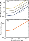Fig. 1 Planetary mass (top) and the Mach number (bottom) as a function of the orbital radius. For the conversion, we assumed a typical steady accretion disk model with a dimensionless viscous alpha parameter (Shakura & Sunyaev 1973), αacc, including viscous heating and stellar irradiation (e.g., Ida et al. 2016). In this model, the aspect ratio is given by h = max(0.027(a/1 au)1/20, 0.024 (a/1 au)2/7), where a solar-mass star, a solar luminosity, the typical accretion rate of classical T Tauri stars, 10−8 M⊙ yr−1, and αacc = 10−3 were assumed (Appendix A).

2.2 Methods of three-dimensional hydrodynamical simulations

Assuming a compressible, inviscid sub-Keplerian gas disk, we performed nonisothermal hydrodynamical simulations. These simulations were performed in the spherical polar coordinates, (r, θ, ϕ), co-rotating with a planet. The numerical resolution was [log r, θ, ϕ] = [128, 64, 128]. The Bondi and Hill radii are resolved by 38–88 and 69–101 cells in the radial direction in our hydrodynamical simulations. We used a free-slip condition at the inner boundary, r = r_inn. Assuming the density of the planetary core to be ρ_pl = 5 g cm⁻³ and the solar-mass star, the size of the inner boundary was set to follow a mass-radius relationship of the planetary core (Kuwahara & Kurokawa 2020a): $$r_{\text{inn}}={\left(\frac{3M_{\text{pl}}}{4\pi {\rho }_{\text{pl}}}\right)}^{1/3}H=3\times {10}^{-2}{m}^{1/3}H{\left(\frac{a}{0.1\text{au}}\right)}^{-1}\equiv r_{\text{inn},0}.$$(3)

We adopted a = 0.1 in Eq. (3) in our fiducial runs. We confirmed the size of the inner boundary does not affect our results (Appendix B). Thus, when we convert the dimensionless quantity into a dimensional one, we can use an arbitrary orbital radius. As the initial state of the disk, we assumed the vertical stratification of the gas density, ρ_g = ρ_∞ exp[−(z/2)²]. The initial gas velocity is υ_g = υ_∞ = (−3x/2 − ℳ_hw)e_y, where υ_g = (υ_x,g, υ_y,g, υ_z,g) is the gas velocity in the local Cartesian coordinates centered at the planet. The internal and total energies of the gas are given by U = p/(γ − 1) and $E=U+{\rho }_{\text{g}}{\upsilon }_{\text{g}}^2/2$, respectively, where γ = 1.4 is the adiabatic index. At the outer boundary, r = r_out, we fixed the gas density and velocity, ρ_g = ρ_∞ and υ_g = υ_∞. Hereafter we denote with the x-, y-, and z-directions the radially outward, azimuthal, and vertical directions to the disk, respectively.

We solved the continuity, Euler’s, and energy conservation equations using Athena++ code² (White et al. 2016; Stone et al. 2020). The external force in Euler’s equation includes the Coriolis force, F_cor = −2e_z × υ_g, the tidal force, F_tid = 3xe_x − ze_z, the global pressure force due to the sub-Keplerian motion of the gas, F_hw = 2ℳ_hwe_x, and the gravitational force (e.g., Ormel et al. 2015b): $$F_{\text{grav }}=-\nabla \left(\frac{m}{\sqrt{r^2+r_{\text{sm}}^2}}\right)\left\{1-\exp \left[-\frac{1}{2}{\left(\frac{t}{t_{\text{inj}}}\right)}^2\right]\right\},$$(4)

where $r=\sqrt{x^2+y^2+z^2}$ is the distance from the planet, r_sm is the smoothing length, and t_inj is the injection time. We set r_sm = 0.1 R_grav for our fiducial runs, where R_grav ≡ min(R_Bondi, R_Hill) is the radius of the gravitational sphere of the planet. We investigated the effect of the smoothing length in Appendix C.

Our simulations utilized the β cooling model, where the radiative cooling occurs on a finite timescale, β (Gammie 2001). The gas is heated by adiabatic compression. Following Kurokawa & Tanigawa (2018), we assumed that the typical scale of the temperature perturbation can be estimated by the Bondi radius, R_Bondi = mH. The dimensionless cooling time can be described by $$\beta ={\left(\frac{m}{0.1}\right)}^2\equiv {\beta }_0$$(5)

which represents the cooling time near the outer edge of the envelope, ~R_Bondi (Kurokawa & Tanigawa 2018). We list our parameter sets in Table 1. We set β = β₀ for our fiducial runs. We investigated the effect of ßin Sect. 5.4.

2.3 Hydrodynamical simulation results

This section summarizes the hydrodynamical simulation results. Based on the numerical results, an analytic formulation of the flow field is presented in Sect. 3.

2.3.1 Summary of three-dimensional planet-induced gas flow

First, we summarize the general properties of the three-dimensional gas flow as reported in previous studies. Planets embedded in disks perturb the surrounding gas and induce the three-dimensional gas flow (Fig. 2; e.g., Ormel et al. 2015b; Fung et al. 2015). The fundamental features of the gas flow around the planet are as follows: (1) the Keplerian shear flow extends inside and outside the orbit of the planet (the green lines of Fig. 2a). (2) The horseshoe flow exists in the anterior-posterior direction of the orbital path of the planet (the orange lines of Fig. 2a). The horseshoe streamlines have a columnar structure in the vertical direction (Fung et al. 2015; Masset & Benítez-Llambay 2016). (3) An isolated inner envelope forms within the gravitational sphere of the planet, r ≲ R_grav, due to the buoyancy barrier (Kurokawa & Tanigawa 2018). We refer to this isolated envelope as an atmosphere. (4) Gas from the disk enters the gravitational sphere of the planet (inflow) and exits (outflow; the red line of Fig. 2a). Following Ormel et al. (2015b) and Kuwahara et al. (2019), we refer to this flow as the recycling flow³. The recycling flow passes the planet, tracing the surface of the atmosphere.

The outflow of the gas occurs in the radial direction to the disk along the recycling streamlines. The following sections (Sects. 2.3.2 and 2.3.3) show the gas flow speed perturbed by the planet at the midplane. We focus especially on the gas flow in the x-direction (the radial gas flow with respect to the disk), which affects both the dust accretion onto the planet and the radial drift of dust. In the following paragraphs, we present a detailed analysis of gas flow speed at the midplane enabled by our extensive parameter studies.

2.3.2 Gas flow speed at the midplane: Dependence on planetary mass

Figure 3 shows the structure of the planet-induced gas flow at the midplane for different planetary masses, m = 0.05, 0.1, 0.5, and 0.7. We set ℳ_hw = 0. The outflow occurs along the inner-leading and outer-trailing recycling streamline (in the second and fourth quadrants of the x–y plane). The streamlines (the thin gray lines in Fig. 3) were plotted with the matplotlib.pyplot.streamplot library, where we used the midplane gas velocities interpolated by the bilinear interpolation method (Appendix D). We highlighted the widest horseshoe streamline and the shear streamline passing closest to the planet (the thick solid and dashed gray lines in Fig. 3; Appendix E). Since we assumed no headwind in Fig. 3, the flow morphology (the shapes of streamlines) are common in all panels. However, the gas velocity changes with the planetary mass. In particular, the x-component of the gas velocity along the inner-leading and outer-trailing recycling streamline (in other words, the outflow speed in the x-direction, υ_x,out, which is the main focus of this study) shows the complex dependence on the planetary mass. When m ≲ 0.5, υ_x,out increases with the planetary mass (Figs. 3a– c), but it seems to decrease for a higher-mass planet (Fig. 3d). From the analytic point of view, we discuss again the dependence of υ_x,out on the planetary mass in Sect. 4.1.1..

2.3.3 Gas flow speed at the midplane: Dependence on headwind

Figure 4 shows the dependence of the gas flow structure on the headwind of the gas for a fixed planetary mass, m = 0.2.

The headwind of the gas breaks a rotational symmetric structure of the planet-induced gas flow (Ormel et al. 2015b; Kurokawa & Tanigawa 2010). The corotation radius for the gas, x_cor,g = −2ℳ_hw/3, shifts in the negative direction on the x-axis as ℳ_hw increases, and the horseshoe region that formed around x = x_cor,g also shifts in the negative x-direction. As shown in Fig. 4, the outflow speed toward the inside (outside) of the planetary orbit decreases (increases) as ℳ_hw increases. From the analytic point of view, we discuss again the dependence of υ_x,out on the Mach number of the headwind in Sect. 4.1.2.

3 Derivation of analytic formulae

Based on the numerical results obtained in Sect. 2.3, here we derive the analytic formulae describing the flow morphology, the maximum outflow speed, and the distributions of the velocity component of the outflow in the radial and vertical directions to the disk.

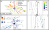Fig. 2 Streamlines of gas flow around the planet with m = 0.05 and ℳhw = 0.03. The arrows represent the direction of the gas flow. Panel a: perspective view of the flow field. Different colors correspond to different types of streamlines. The size of the atmosphere is 0.04 H. Panel b: same as panel a, but the color contour represents p/ρg, which is the measure of temperature (Sect. 3.3). Panel c: x-y plane viewed from the +z-direction. The critical streamline is highlighted by the color contour, which represents Bernoulli’s function, ℬ (Sects. 3.3 and 5.3).

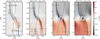Fig. 3 Dependence of the planet-induced gas flow on the planetary mass at the midplane. We set ℳhw = 0 in all panels. The results were obtained from m005-hw0 (panel a), m01-hw0 (panel b), m05-hw0 (panel c), and m07-hw0 (panel d). The solid thin gray lines are gas streamlines. The solid and thick dashed gray lines are the widest horseshoe streamline and the shear streamline passing closest to the planet, respectively (Appendix E). The color contour represents the flow speed in the x-direction. The dashed and dashed-dotted black circles denote the atmospheric radius (Eq. (5)) and twice the atmospheric radius, where the outflow speed is measured. The dashed blue lines are the curves representing the fitting formula for the critical recycling streamline (Eq. (11); Sect. 3.2.1). The vertical lines are the asymptotes of Eq. (11), representing the extent of the outflow region in the x-direction ((Eq. (17)); Sect. 3.2.2). The horizontal lines denote the y-coordinates of the characteristic length of the outflow region in the y-direction ((Eq. (18)); Sect. 3.2.3).

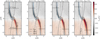Fig. 4 Same as Fig. 3, but showing the dependence of the planet-induced gas flow on the Mach number of the headwind. We set m = 0.2 in all panels. The results were obtained from m02-hw0 (panel a), m02-hw001 (panel b), m02-hw003 (panel c), and m02-hw01 (panel d). The vertical dotted line corresponds to the corotation radius for the gas.

3.1 Atmospheric radius

The size of an atmosphere affects gas dynamics around an embedded planet, because the recycling streamlines trace the surface of the atmosphere (Fig. 2). Hereafter, we define the size of the atmosphere as the atmospheric radius, the maximum radius where the azimuthal gas velocity is dominant in the midplane region (Moldenhauer et al. 2022): $$R_{\text{atm}}\equiv \max \left(r{\left|v_{\varphi ,\text{g}}\right|}_{\text{midplane }}>\max \left(v_{r, \text{g}},v_{\theta ,\text{g}}\right)\right)$$(6)

where υ_g = (υ_r,g, υ_θ,g, υ_ϕ,g) is the gas velocity in the spherical polar coordinates centered at the planet. To estimate the atmospheric radius, we used the final state of the hydro-simulations data, t = t_end, where the flow field seems to have reached a steady state (Appendix F).

Figure 5 shows the dependence of the atmospheric radius on the planetary mass and the Mach number of the headwind. We find that the atmospheric radius scales with the Bondi or Hill radii. The headwind of the gas reduces the atmospheric radius for a fixed planetary mass, which is consistent with previous studies (Ormel 2013; Moldenhauer et al. 2022). Assuming that the atmospheric radius decreases linearly as ℳ_hw increases, we introduce a fitting formula for the dimensionless atmospheric radius as $$R_{\text{atm},\text{fit}}\equiv \min \left(C_1{R}_{\text{Bondi}}-D_1{ℳ}_{\text{hw}},C_2{R}_{\text{Hill}}-D_2{ℳ}_{\text{hw}}\right)$$(7)

where C₁, C₂, D₁, and D₂ are the fitting coefficients. With the least-squares method, we determined the values of these coefficients: C₁ = 0.84, C₂ = 0.36, D₁ = 0.056, and D₂ = 0.22. The atmospheric radii are resolved by 28–52 cells in the radial direction in our hydrodynamical simulations.

The atmospheric radius can be constrained by the thermo-dynamical condition or the planet’s gravity, namely, the Bondi radius or the Roche lobe radius of the planet, whichever is smaller (D’Angelo & Lubow 2008; D’Angelo & Bodenheimer 2013). The Roche lobe is surrounded by the equipotential surface of the so-called Roche potential. Although the Roche lobe is not spherical, the radius of a sphere having the same volume as the Roche lobe is given by the following fitting formula (Eggleton 1983): $$R_{\text{Roche }}=\frac{0.49m^{2/3}h}{0.6m^{2/3}{h}^2+\ln \left(1+m^{1/3}h\right)}H\text{. }$$(8)

For a typical steady accretion disk model (e.g., Ida et al. 2016), the disk aspect ratio has on the order of h ~ 0.01−0.1 (Appendix A). The value of R_Roche hardly changes for the range of h. We set h = h₀ = 0.05 as a nominal value in Eq. (8). Since m^1/3h ≪ 1 in our parameter sets, Eq. (8) can be approximated as R_Roche ≃ 0.49m^1/3 H ~ 2R_Hill/3 (Paczynski 1971), where we used ln(1 + m^1/3h) ≃ m^1/3h and (1 + 0.6m^1/3h) ≃ 1. We plotted the following equation in Fig. 5: $$R_{\text{atm,lim }}=\min \left(R_{\text{Bondi }},R_{\text{Roche }}\right)\text{. }$$(9)

Equation (9) predicts that the scaling law changes at m ~ 0.3 and the atmospheric radius scales with ~2R_Hill/3 when m ≳ 0.3. These predictions are in qualitative agreement with the numerical result where the atmospheric radius scales with a fraction of the Hill radius when m ≳ 0.2.

The gas is heated by adiabatic compression and then the β cooling occurs within the gravitational sphere of the planet, leading to the formation of the low-entropy region at r ≲ R_grav (Fig. 6a; Kurokawa & Tanigawa 2018). The buoyancy force characterized by the positive entropy gradient isolates the atmosphere from the surrounding disk gas (Kurokawa & Tanigawa 2018). We find that the temperature is nearly uniform around the atmosphere due to our choice of short cooling time when m ≲ 0.1 (β ≤ 1; Fig. 6b). The amplitude of the temperature fluctuation increases with the planetary mass, which is as high as ~75% when m = 1.

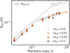Fig. 5 Atmospheric radius as a function of the planetary mass and the Mach number of the headwind of the gas. The square symbols were obtained from hydrodynamical simulations. Different colors correspond to different Mach numbers, ℳhw. The gray-shaded region is given by the fitting formula for the atmospheric radius, Ratm,fit. The dashed gray line is given by Eq. (9).

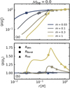Fig. 6 Shell-averaged values of $p/{\rho }_{\text{g}}^{\gamma }$ (panel a) and p/ρg (panel b), which are the measures of the entropy and the temperature, respectively, as a function of the distance from the planet. We set γ = 1.4. Different colors correspond to different planetary masses. The filled circles, the squares, and the triangles denote the atmospheric radius, the Bondi radius, and the Hill radius, respectively. We set ℳhw = 0.

3.2 Morphology of the outflow region

This section introduces the fitting formulae for the morphology of the midplane outflow (the shape of the outflow streamline), describing the region where the x-component of the gas velocity, υ_x,g, is dominantly perturbed by the embedded planet (the deep red and black contours in Figs. 3 and 4). We refer to this region as the outflow region. The obtained formulae will be used in a future study to determine the extent of the region in which the hydrodynamic effects of the outflow on the dust motion would appear. Hereafter we restrict our attention to the limited region, |x| ≲ H and z = 0.

3.2.1 Morphology of the critical recycling streamline at the midplane

The outflow occurs along the recycling streamline, which suggests that the outflow region can be determined by the shape of the recycling streamline. The shape of the streamline is also important to estimate the outflow speed in the x-direction, υ_x,out, which affects the dust motion (Kuwahara & Kurokawa 2020a,b), because υ_x,out can be obtained by considering the angle of the flow velocity with respect to the x-axis.

Here we introduce a representative recycling streamline: a critical recycling streamline. We defined the critical recycling streamline as the separatrix streamline that divides the Keplerian shear flow and the inner-leading (outer-trailing) recycling flow at the midplane. We find that the inner-leading and outer-trailing critical recycling streamlines at the midplane can be outlined by the following fitting formulae: $$\{\begin{array}{lll}r=\hfill & w_{\text{out }}^{+}\tan \theta \hfill & (3\pi /2\le \theta \le 2\pi ),\hfill \\ r=\hfill & w_{\text{out }}^{-}\tan \theta \hfill & (\pi /2\le \theta \le \pi ),\hfill \end{array}$$(10)

in the polar coordinates centered at the planet, where $w_{\text{out}}^{\pm }$ is the x-coordinate of the edge of the outflow region (described in Sect. 3.2.2). The dust motion can be disturbed by the outflow in the region where $w_{\text{out }}^{-}\le x\le w_{\text{out }}^{+}$. Hereafter the plus and minus signs for an arbitrary quantity, X^±, denote the quantity outside and inside the planetary orbit. Equation (10) represents the tangential curves with $w_{\text{out}}^{\pm }$ as the asymptotes. In the local Cartesian coordinates co-rotating with the planet, Eq. (10) can be written as $$y=-\frac{x^2}{\sqrt{{\left(w_{\text{out }}^{+}\right)}^2-x^2}}\mathscr{H}(x)+\frac{x^2}{\sqrt{{\left(w_{\text{out }}^{-}\right)}^2-x^2}}\mathscr{H}(-x)\equiv f_{\text{out }}(x)$$(11)

where 𝓗(x) is the Heaviside step function.

We plotted Eq. (11) in Figs. 3 and 4. Equation (11) can trace the critical recycling streamline at the midplane for a wide range of planetary mass and Mach number of the headwind. In most of the panels in Figs. 3 and 4, f_out(x) is sandwiched between the widest horseshoe streamline and the shear streamline passing closest to the planet. Using Eq. (11), we estimate the outflow speed analytically near the atmospheric radius, R_atm ≲ 0.1 H, where the dominant outflow occurs (Figs. 3 and 4; described in Sect. 3.4). We use the analytically estimated outflow speed for the estimation of the outflow effect on the dust motion. Thus, the agreement between Eq. (11) and the numerically obtained critical recycling streamline in the region close to the planet (r ~ R_atm) is useful. Although Eq. (11) does not coincide with the numerically obtained critical recycling streamline in the distant region far from the planet, |y| ≳ H, the mismatch between Eq. (11) and the numerically obtained critical recycling streamline in the far region does not affect an analytic derivation of the outflow speed.

Equation (11) can be applied to trace the critical recycling streamline near the atmospheric radius for the entire range of our parameter sets (m ∈ [0.03, 1]). When m ≳ 0.6, however, we find that the dominant perturbation to υ_x,g occurs along the midplane horseshoe streamlines rather than the streamlines characterized by Eq. (11) (e.g., Fig. 3d; described in Sect. 4). When the planetary mass reaches the so-called pebble isolation mass, M_iso = 25(h/0.05)³[0.34(3/log α_acc)⁴ + 0.66] M_⊕, a growing planet opens a shallow gas gap (Lambrechts et al. 2014; Bitsch et al. 2018; Ataiee et al. 2018). In our dimensionless unit, the pebble isolation mass can be described as $$m_{\text{iso }}\simeq 0.6\left[0.34{\left(\frac{3}{\log {\alpha }_{\text{acc }}}\right)}^4+0.66\right]{\left(\frac{M_{*}}{M_{\odot }}\right)}^{-1}$$(12)

We assumed α_acc = 10⁻³ and M_* = M_⊙ in Eq. (12) as nominal values. Our local simulation cannot handle the gas-gap opening in the high-mass regime (m ≳ m_iso). Thus, Eq. (11) is valid as a model for the outflow streamline for m ≲ m_iso ≃ 0.6 to investigate the hydrodynamic effect of the gas flow on the dust.

3.2.2 Width of the outflow region

In Sect. 3.2.1, we introduced a fitting formula for the critical recycling streamline, y = f_out(x), which represents the edge of the outflow region whose x-coordinate approaches asymptotically to x =  $w_{\text{out}}^{\pm }$. This section describes the width of the outflow region in the x-direction (the radial direction to the disk) and introduces an analytic description for $w_{\text{out}}^{\pm }$.

We find that the width of the outflow region is limited by the width of the subsonic region and the x-coordinate of the recycling streamline at the midplane characterized by the half-width of the horseshoe streamline. We defined the subsonic region as the region where the unperturbed gas velocity in the local frame is always subsonic, |υ_g,∞| ≤ c_s. The x-coordinate of the edge of the subsonic region for the gas is given by $$x_{\text{subsonic }}^{\pm }\equiv \pm \frac{2}{3}H-\left|x_{\text{cor,g }}\right|\text{\hspace{1em} (double-sign corresponds). }$$(13)

Hereafter we omit the notation of the double-sign corresponds in each equation, unless otherwise specified.

Next, we introduced the x-coordinate of a critical recycling streamline in the far field (|y| → ∞) at the midplane. We started by considering an endmember case, ℳ_hw = 0. The gas from the disk enters the gravitational sphere of the planet and flows back to the disk through the region between the Keplerian shear flow and the inner-leading (outer-trailing) horseshoe flow. Thus, the width of the outflow region could be constrained by the width of the horseshoe flow. When m ≲ 0.1, the half-width of the horseshoe streamline can be estimated by the linear theory, which is given by (Masset & Benítez-Llambay 2016) $$w_{\text{HS}}^{\text{MB}16}=1.05\sqrt{m},$$(14)

combined with the numerical factor. When m ≳ 0.1, the half-width of the horseshoe streamline is proportional to the Hill radius of the planet due to the onset of nonlinear effects in the horseshoe region, which can be fitted by w_HS ≃ 2.4R_Hill ≃ 1.7m^1/3 (Masset et al. 2006). Jiménez & Masset (2017) introduced the following fitting formula for the half-width of the horseshoe streamline, which can be applied to a wide range of planetary masses: $$w_{\text{HS}}^{\text{JM}17}=\frac{1.05\sqrt{m}+3.4m^{7/3}}{1+2m^2}\equiv w_{\text{HS}}.$$(15)

We find that Eq. (15) is a better indicator than Eq. (14) in describing the width of the outflow region for practical use, though it overestimates the widths of the outer-leading and inner-trailing parts of the horseshoe flows (Appendix G).

When the nonzero Mach number of the headwind is assumed, the horseshoe region shifts to the negative direction in the x-axis by −|x_cor,g|. We find that the disk gas along the recycling streamline flows into an empty space formed by the shift of the horseshoe region (Fig. 2a). The critical recycling streamline traces this replenished flow. The x-coordinate of the critical recycling streamline at the midplane in the far field is given by $$x_{\text{rec }}^{\pm }\equiv \pm w_{\text{HS}}\pm \left|x_{\text{cor, g}}\right|.$$(16)

We find that the width of the outflow region in the x-direction can be characterized by x_subsonic (Eq. (13)) or x_rec (Eq. (16)), whichever was smaller: $$w_{\text{out }}^{\pm }=\pm \min \left(\left|x_{\text{subsonic }}^{\pm }\right|,\left|x_{\text{rec }}^{\pm }\right|\right)\text{. }$$(17)

We plotted Eq. (17) in Figs. 3 and 4, which can serve as a useful guide for the extent of the region where υ_x,g is dominantly perturbed by the embedded planet.

Figure 7 shows the difference of the flow speed from the unperturbed sub-Keplerian speed, where m = 0.1 and 0.5, and ℳ_hw = 0 were assumed. When |x_rec| < |x_subsonic| (m ≲ 0.3; for simplicity, we omit the plus and minus signs), the gas velocity approaches the unperturbed sub-Keplerian shear when x → x_rec, leading to υ_x,g → 0 (Fig. 7a). When |x_rec| > |x_subsonic| (m ≳ 0.3), the numerically obtained critical recycling streamline can intrude the supersonic region because its width is determined by x_rec (= |w_HS| > |x_subsonic|; the solid orange lines in Fig. 7b). However, υ_x,g along the numerically obtained critical recycling streamline approaches instantaneously to υ_x,g → 0 in the subsonic region (Fig. 7b). Since we defined the outflow region as the region where υ_x,g is dominantly perturbed by the planet, we considered that the outflow region is constrained by w_out = |x_subsonic|, regardless of the x-coordinate of the numerically obtained critical recycling streamline at |y| ≳ L_y,out ≃ H. Although a mismatch between the numerically obtained critical recycling streamline and f_out(x) can be seen at |y| ≳ H, again, it does not affect an analytic derivation of the outflow speed.

3.2.3 Length of the outflow region

In this section, we evaluate the characteristic length of the outflow region in the y-direction (the orbital direction of the planet). The extent of the outflow region in the y-direction can be used when we investigate the outflow effects on the dust motion during the encounter with the planet. Based on Eq. (11), we define the y-coordinate at a position close enough to the asymptotes, $x=w_{\text{out}}^{\pm }$, as the characteristic length of the outflow region: $$L_{y,\text{ out }}^{\pm }\equiv f_{\text{out }}\left(x_{\text{crit }}^{\pm }\right),$$(18)

where $$x_{\text{crit }}^{\pm }=C_{\text{crit }}\times w_{\text{out }}^{\pm }.$$(19)

We set C_crit = 0.95 as a fitting parameter. We plotted Eq. (18) in Figs. 3 and 4, which shows good agreement with numerical simulations.

3.3 Bernoulli’s theorem

The outflow speed can be estimated from Bernoulli’s theorem (Fung et al. 2015; Kuwahara et al. 2019). For a steady-state barotropic flow, a Bernoulli function is conserved along a streamline (Ormel 2013; Fung et al. 2015; Kuwahara et al. 2019): $$ℬ=\frac{v_{\text{g}}^2}{2}+-2{ℳ}_{\text{hw}}x+{\Phi }_{\text{eff}},$$(20)

where 𝒫 = ∫ dp/ρ_g is the pressure function and Φ_eff is the effective potential. Here we assume an isothermal flow along a recycling streamline, $p={\rho }_{\text{g}}{c}_{\text{s}}^2$. The pressure function is described by $P=c_{\text{s}}^2$ ln ρ_g. The effective potential is described by $${\Phi }_{\text{eff}}=-\frac{3}{2}{x}^2+\frac{z^2}{2}-\frac{m}{r},$$(21)

where the first and second terms in the right-hand side of Eq. (21) were originated from the tidal potential.

It should be noted that Bernoulli’s function does not strictly conserve along the streamline as shown in Fig. 2c, because the β cooling occurs on a finite timescale, β = (m/0.1)². However, we find that Bernoulli’s theorem is still useful to estimate the outflow speed because the gas flow along a recycling streamline can be considered as an isothermal flow due to the efficient β cooling (Fig. 6b). As discussed in Sect. 3.1, when m ≲ 0.1 the temperature around the atmosphere is nearly uniform (Fig. 6b). Although the amplitude of the temperature fluctuation around the atmosphere is as high as ~40% at most when m ~ m_iso, we stick to an isothermal assumption regardless of the planetary mass. Again, our model for the outflow speed is not valid in the higher-mass regime (m ≳ m_iso; Sect. 3.2.1). We discuss the applicability of Bernoulli’s theorem in Sect. 5.3.

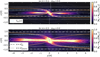Fig. 7 Difference of the flow speed from the unperturbed Keplerian shear. The results were obtained from m01 − hw0 (panel a) and m05 − hw0 (panel b). The dashed blue, dashed-dotted white, and dotted white lines denote the fitting formula for the critical recycling streamline, the x-coordinate of the critical recycling streamline at the midplane in the far field, and the x-coordinate of the edge of the subsonic region, respectively. As in Fig. 3, we highlight the widest horseshoe streamline and the shear streamline passing closest to the planet with the solid and dashed orange lines, respectively.

3.4 Inflow and outflow positions

To estimate the outflow speed from Bernoulli’s theorem, following Kuwahara et al. (2019), we select a recycling streamline and set the inflow and outflow points on it, P_in and P_out, where the gas chiefly flows in and out. These points are determined by the analysis of the mass flux of the gas.

The left column of Fig. 8 shows the velocity field of the gas at the meridian plane, in which the color contour corresponds to the radial velocity in the spherical polar coordinates centered at the planet. The gas seems to be dominantly flowing in and out of the sphere of radius ≳2 R_atm. The right column of Fig. 8 shows the azimuthally averaged mass flux for a certain spherical shell of radius r, 〈ρ_gυ_r,g〉_ϕ, as a function of the altitude, z. Gas flows in where 〈ρ_gυ_r,g〉_ϕ < 0 and flows out where 〈ρ_gυ_r,g〉_ϕ > 0. We find that gas chiefly flows in and out of twice the atmospheric radius, 2 R_atm.

Based on the above findings, we set the inflow and outflow points as P_in = (0, 0, z_in) and $P_{\text{out}}^{\pm }=\left(x_{\text{out}}^{\pm },y_{\text{out}}^{\pm },0\right)$, where z_in = 2 R_atm,fit and 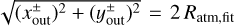$\sqrt{{\left(x_{\text{out }}^{\pm }\right)}^2+{\left(y_{\text{out }}^{\pm }\right)}^2}=2R_{\text{atm, fit }}$. Here we used a fitting formula for the atmospheric radius (Eq. (7)). The x- and y-coordinates of the outflow points were determined by those of the intersections of the fitting formula for the critical recycling streamline at the midplane (Eq. (11)) and the circle of twice the atmospheric radius, 2 R_atm,fit. They are given by $$x_{\text{out }}^{\pm }=\pm 2R_{\text{atm, fit }}\cos \left({\tan }^{-1}\left(\frac{2R_{\text{atm, fit }}}{w_{\text{out }}^{\pm }}\right)\right)\text{, }$$(22) $$y_{\text{out }}^{\pm }=f_{\text{out }}\left(x_{\text{out }}^{\pm }\right)\text{. }$$(23)

3.5 Analytic formula for the outflow speed

An analytic formula of the outflow speed was derived from Bernoulli’s theorem. We first consider the inflow point. From the analysis of the kinetic energy of gas flow in our simulations, we find that the first term in the right-hand side of Eq. (20) was negligible at the inflow point, P_in (Fung et al. 2015; Kuwahara et al. 2019). The second and fourth terms in the right-hand side of Eq. (20) are canceled with each other because the stellar gravitational potential energy balances the pressure function in hydrostatic equilibrium. Thus, Bernoulli’s function at the inflow point is described by $${ℬ}_{\text{in }}=-\frac{m}{2R_{\text{atm, fit }}}$$(24)

Bernoulli’s function at the outflow point is described by $${ℬ}_{\text{out }}^{\pm }=\frac{{\left(v_{\text{out }}^{\pm }\right)}^2}{2}-\frac{3}{2}{\left(x_{\text{out }}^{\pm }\right)}^2-2{ℳ}_{\text{hw}}{x}_{\text{out }}^{\pm }-\frac{m}{2R_{\text{atm, fit }}}$$(25)

From Eqs. (24) and (25), we obtain the outflow speed at the outflow point: $$\left|v_{\text{out }}^{\pm }\right|=\sqrt{3{\left(x_{\text{out }}^{\pm }\right)}^2+4{ℳ}_{\text{hw }}{x}_{\text{out }}^{\pm }}.$$(26)

The first and second terms in the square root in the right-hand side of Eq. (26) originate from the tidal potential (Kuwahara et al. 2019) and the global pressure gradient of the disk gas, respectively.

From Eq. (26), we can estimate the flow speed in the x-direction (the radial flow speed with respect to the disk), which affects both the dust accretion onto the planet and the radial drift of dust. The x-component of the outflow speed is given by $$v_{x,\text{ out }}^{\pm }=\left|v_{\text{out }}^{\pm }\right|\cos {\phi }_{\text{out }}^{\pm },$$(27)

where ${\phi }_{\text{out }}^{\pm }$ is an angle of the outflow to the x-axis at the outflow point, $${\phi }_{\text{out }}^{\pm }={{\tan }^{-1}\left(\frac{\text{d}{f}_{\text{out }}(x)}{\text{d}x}\right)|}_{x=x_{\text{out }}^{\pm }}\text{, }$$(28)

which can be described by $$\{{\phi }_{\text{out }}^{+}={\tan }^{-1}\left[-\frac{x_{\text{out }}^{+}\left(2{\left(w_{\text{out }}^{+}\right)}^2-{\left(x_{\text{out }}^{+}\right)}^2\right)}{{\left({\left(w_{\text{out }}^{+}\right)}^2-{\left(x_{\text{out }}^{+}\right)}^2\right)}^{3/2}}\right],$$(29) $$\{{\phi }_{\text{out }}^{-}={\tan }^{-1}\left[\frac{x_{\text{out }}^{-}\left(2{\left(w_{\text{out }}^{-}\right)}^2-{\left(x_{\text{out }}^{-}\right)}^2\right)}{{\left({\left(w_{\text{out }}^{-}\right)}^2-{\left(x_{\text{out }}^{-}\right)}^2\right)}^{3/2}}\right]\text{. }$$(30)

We compare Eq. (27) with the numerical results in Sect. 4.1.

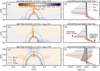Fig. 8 Gas flow structure and azimuthally averaged mass flux. The results were obtained from m02 − hw0 (panels a and b), m02 − hw01 (panels c and d), and m04 − hw0 (panels e and f). Left column: gas flow structure at the meridian plane. The color contour represents the r-component of the gas velocity in the spherical polar coordinates centered at the planet and averaged in the y-direction within the calculation domain of the hydrodynamical simulation. The dashed, dotted, and dashed-dotted circles denote the Bondi radius, the Hill radius, and twice the atmospheric radius, respectively. Right column: mass flux of the gas averaged in the azimuthal direction in the spherical polar coordinates centered at the planet, 〈ρgυr〉ϕ. Each solid line represents the changes in 〈ρgυr〉ϕ; altitude is varied along with a certain radius. We highlight the important radii with solid yellow (RBondi), blue (RHill), and red (2 Ratm) lines.

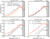Fig. 9 Outflow speed at the midplane as a function of the dimensionless planetary mass and the Mach number of the headwind of the gas. The star symbols were obtained from hydrodynamical simulations, corresponding to the maximum flow speeds in the x-direction toward the outside (red) and inside (black) of the planetary orbit within the limited region, $w_{\text{out }}^{-}\le x\le w_{\text{out }}^{+},L_{\text{out }}^{-}\le y\le L_{\text{out }}^{+}$, and $\sqrt{x^2+y^2}\ge R_{\text{atm }}$. The last condition avoids incorrectly sampling the large υx,g within the atmosphere. The solid red and black lines correspond to the analytic formulae for the x-components of the outflow speeds (Eq. (27)). The dashed lines correspond to the analytic formulae for the outflow speed in the x-direction obtained by Ormel (2013, blue; Eq. (38)), Fung et al. (2015, purple; Eq. (41)), and Kuwahara et al. (2019, yellow; Eq. (43)). The gray shading marks the region where the planetary mass exceeds the pebble isolation mass, miso (Eq. (12)).

3.6 Analytic formula for the velocity distribution of the outflow

We derive analytic formulae for υ_x,out(x) and υ_x,out(z). These formulae are useful for modeling the influence of the outflow on the radial drift of dust in disks for the following reasons: (1) Dust particles drift from the outside to the inside of the planetary orbit. The radial drift of dust can be disrupted by the gas flow, leading to the formation of a dust substructure such as a dust ring and a gap (Kuwahara et al. 2022). (2) The dust is stirred up by the gas turbulence, leading to an increase in the dust scale height (e.g., Youdin & Lithwick 2007). Thus, the influence of the gas flow on the dust motion depends on the vertical structure of the planet-induced gas flow.

3.6.1 Radial direction to the disk

The outflow region has a spread in the x-direction with the width of $w_{\text{out}}^{\pm }$. Here we aim to model the distribution of υ_x,out in the x-direction at the midplane, υ_x,out(x). We find that υ_x,out(x) can be modeled by a Gaussian function with peaks at $x=x_{\text{out}}^{\pm }$. We introduce the following formula: $$v_{x,\text{ out }}(x)=v_{x,\text{ out }}^{+}\exp \left[-\frac{{\left(x-x_{\text{out }}^{+}\right)}^2}{2{\left(D^{+}\right)}^2}\right]-v_{x,\text{ out }}^{-}\exp \left[-\frac{{\left(x-x_{\text{out }}^{-}\right)}^2}{2{\left(D^{-}\right)}^2}\right],$$(31)

where we assumed that the full width at half maximum (FWHM) corresponds to the half-width of the outflow region, $\text{FWHM\hspace{0.17em}=\hspace{0.17em}}2\sqrt{2\ln 2}{D}^{\pm }=w_{\text{out }}^{\pm }/2$. We compare Eq. (31) with the numerical results in Sect. 4.2.

3.6.2 Vertical direction to the disk

The outflow has a vertical extent as shown in the left column of Fig. 8. The outflow speed decreases sharply at z ≳ R_atm. Assuming that υ_x,out(z) decreases exponentially when z > R_atm,

we introduce the following formula: $$\begin{array}{l}{v}_{x,\text{out}}^{\pm }(z)={{\langle v_{x,\text{g}}^{\pm }\rangle }_{x,y}|}_{z=0}\times \exp \left[-{\left(\frac{z}{R_{\text{atm}}}\right)}^2\right],\\ ={\frac{{\displaystyle \int \text{}}\text{}{\displaystyle \int {\rho }_{\text{g}}}{v}_{x,\text{g}}^{\pm }\text{d}x\text{d}y}{{\displaystyle \int \text{}}\text{}{\displaystyle \int {\rho }_{\text{g}}}\text{d}x\text{d}y}|}_{\text{z}=0}\times \exp \left[-{\left(\frac{z}{R_{\text{atm}}}\right)}^2\right].\end{array}$$(32)

We used the numerical results to compute the integral in the right-hand side of Eq. (32). We compare Eq. (32) with the numerical results in Sect. 4.2.

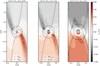Fig. 10 Comparison of the point where υx,g has the maximum value at the midplane and the assumed outflow point, $P_{\text{out}}^{\pm }$ (the open circle on the dashed-dotted circle). The results were obtained from m02 − hw003 (panel a), m05 − hw0 (panel b), and m1 − hw0 (panel c). The star symbols denote the points where the flow speed in the positive (the red star) and the negative (the black star) x-direction has the maximum value in the limited region, $w_{\text{out }}^{-}\le x\le w_{\text{out }}^{+},L_{\text{out }}^{-}\le y\le L_{\text{out }}^{+}$ (the ranges of the x- and y-axes of these panels), and $\sqrt{x^2+y^2}\ge R_{\text{atm}}$. The flow speed at the star symbol was plotted in Fig. 9a with the same color star symbol.

4 Comparison to numerical results

In this section, we compare our analytic formulae for the outflow speed obtained in Sect. 3 with the numerical results.

4.1 Maximum outflow speed at the midplane

Figure 9 compares our analytic formula for the x-component of the outflow speed (Eq. (27)) with the maximum flow speed in the x-direction obtained from hydrodynamical simulations, υ_x,max. Equation (27) reproduces the results obtained from hydrodynamical simulations for a wide range of planetary mass and Mach number of the headwind of the gas.

It should be noted that the point where |υ_x,g| has the maximum value, $P_{\max }^{\pm }$, does not necessarily coincide with the assumed outflow point, $P_{\text{out}}^{\pm }$, which is determined by the analysis of the azimuthally averaged mass flux (Fig. 10). Figure 11 shows the mismatch between υ_x,max and υ_x,g at the assumed outflow point, $P_{\text{out}}^{\pm }$, meaning that flow speed at the exact location as the analytically-predicted outflow point does not take the maximum value. This is because the fitting formula for the critical recycling streamline, f_out(x), does not trace a streamline, which gives the maximum flow speed at the midplane region. The fitting formula, ƒ_out(x), traces the edge of the outflow region where υ_x,g is dominantly perturbed (e.g., Fig. 10a). It almost coincides with the shear streamline passing closest to the planet near the atmosphere. The assumed outflow point, $P_{\text{out}}^{\pm }$, is located at the point very close to the intersection of the shear streamline and the circle of twice the atmospheric radius, where the perturbation to υ_x,g along the shear streamline is small (Fig. 10). Thus, the flow speed obtained from hydrodynamical simulations at $P_{\text{out}}^{\pm }$ deviates from the maximum value (Fig. 11).

We find that $P_{\text{max}}^{\pm }$ lies on a circle of radius ~1.6–4 R_atm with no clear trend in the location of $P_{\text{max}}^{\pm }$ as a function of the planetary mass and the Mach number of the headwind (Fig. 10). We find that the error between the maximum value of υ_x,g on a circle of radius 2R_atm and υ_x,max is less than 30%. Thus, twice the atmospheric radius can still be considered as the radius where the dominant outflow occurs. For simplicity, we stick to setting $\sqrt{{\left(x_{\text{out}}^{\pm }\right)}^2+{\left(y_{\text{out}}^{\pm }\right)}^2}=2R_{\text{atm},\text{fit}}$ for the derivation of outflow speed.

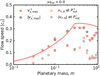Fig. 11 Comparison of the maximum flow speed in the x-direction, ${\upsilon }_{x,\max }^{\pm }$, and υx,g at the analytically assumed outflow point, $P_{\text{out}}^{\pm }$. We set ℳhw = 0.

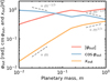Fig. 12 Angle of the outflow at the outflow point, φout (Eq. (28)), cos φout, and the x-coordinate of the outflow point, $x_{\text{out}}^{\pm }$ (Eq. (23)) as a function of the planetary mass. We set ℳhw = 0.

4.1.1 Revisiting the dependence on planetary mass

Based on Fig. 9, we revisit the dependence of υ_x,out on the planetary mass as mentioned in Sect. 2.3.2. The outflow speed in the x-direction, υ_x,out, has a peak when m ~ 0.3, corresponding to a super-Earth mass planet at 1 au for a typical steady accretion disk model. From the analytic point of view, this trend can be understood by considering the dependence of the outflow angle on the planetary mass (Fig. 12). In this section, we only consider the shear only case (ℳ_hw = 0) for simplicity.

When m ≲ 0.3, the outflow speed is proportional to |υ_out| ∝ x_out ∝ R_atm,fit ∝ m (Eq. (26)). We find that the cosine term in Eq. (27), cos φ_out, is proportional to ~m^−1/3 (Fig. 12). Thus, the outflow speed in the x-direction is almost proportional to ${\upsilon }_{x\text{,out}}^{\pm }\propto$ m^2/3. When m ≳ 0.3, the dependence of the outflow speed on the planetary mass is slightly lower than the power of 1/3 due to the cosine term in Eq. (23), $\cos \left({\tan }^{-1}\left(2R_{\text{atm},\text{fit}}/w_{\text{out}}^{\pm }\right)\right)$ (Fig. 12). The cosine term in Eq. (27), cos φ_out, is proportional to ~m^−1/3 (Fig. 12). Thus, υ_x,out decreases as the planetary mass increases.

Our analytic formula deviates from the results obtained by hydrodynamical simulations when m ≳ 0.6 (Fig. 9). For such higher-mass planets, we find that $P_{\text{max}}^{\pm }$ is located at the region close to the planetary orbit (Fig. 10b). In Fig. 10b, υ_x,g has the maximum value on the midplane horseshoe streamline, not on the critical recycling streamline. Thus, the flow speed cannot be estimated by Eq. (27). As discussed in Sect. 3.2.1, our model for the critical recycling streamline can be applied when m ≲ m_iso ≃ 0.6. Thus, our analytic formula for the outflow speed is also valid when m ≲ m_iso. We plotted m_iso (Eq. (12)) in Fig. 9.

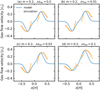Fig. 13 Distribution of the x-component of the gas velocity in the x-direction at the midplane, υx,max(x). The solid blue line is given by Eq. (31). The yellow dots were obtained from m02-hw0 (panel a), m02-hw001 (panel b), m02-hw003 (panel c), and m02-hw01 (panel d). We sampled the gas velocity at each radial grid of hydro-dynamical simulations where the absolute value of the gas velocity was the maximum within the limited region, $w_{\text{out }}^{-}\le x\le w_{\text{out }}^{+},L_{\text{out }}^{-}\le y\le L_{\text{out }}^{+}$, and $\sqrt{x^2+y^2}\ge R_{\text{atm}}$.

4.1.2 Revisiting the dependence on headwind

Based on Fig. 9, we revisit the dependence of υ_x,out on the Mach number of the headwind, ℳ_hw, as mentioned in Sect. 2.3.3. The outflow speed in the x-direction toward the inside (outside) of the planetary orbit decreases (increases) as ℳ_hw increases. This is caused by the second term in the square root in the right-hand side of Eq. (26), which comes from the global pressure force due to the sub-Keplerian motion of the gas, F_hw = 2ℳ_hwe_x. Since the gas receives the global pressure force in the positive direction in the x-axis, the outflow toward the inside (outside) of the planetary orbit is reduced (enhanced).

When ℳ_hw = 0.1, the strongest Mach number considered in this study, our analytic formula deviates from the results obtained by hydrodynamical simulations inside the planetary orbit. We speculate that the deviation was caused by the changes of the actual location of the inflow point, P_in. To obtain the analytic formula for the outflow speed, we set P_in at the pole of the spherical shell of the radius 2 R_atm,fit regardless of the assumed ℳ_hw. In reality, P_in shifts to the negative direction in the x-axis as ℳ_hw increases (Fig. 8b), because the horseshoe flow shifts to the negative direction in the x-axis. However, as long as we consider the influence of the outflow on the radial drift of dust, the outflow toward the inside of the planetary orbit is less important than that toward the outside the planetary orbit.

4.2 Velocity distribution of the outflow

Figure 13 shows υ_x,out(x) at the midplane obtained from both our analytic formula (Eq. (31)) and hydrodynamical simulations.

We set m = 0.2 and varied the Mach number of the headwind, ℳ_hw = 0–0.1 in Fig. 13. We find that Eq. (31) can reproduce the trends of the hydro-simulations results: the peak speed, the FWHM, and the x-coordinate of the peak position.

Figure 14 shows υ_x,out(z) for different planetary masses, m = 0.2, and 0.5, and Mach numbers, ℳ_hw = 0, and 0.1. The left column of Fig. 14 shows the vertical structure of the gas flow field at the meridian plane obtained from hydrodynamical simulations. The gas flow velocity was averaged in the y-direction within the calculation domain of hydrodynamical simulation. The right column of Fig. 14 shows υ_x,out(z) obtained from both the numerical result and our analytic formula. The numerical result was obtained by averaging the simulation data as $${\text{υ}}_{x,\text{ out }}^{\text{num }}(z)\equiv {\langle {\text{υ}}_{x, \text{g}}^{\pm }(z)\rangle }_{x,y}=\frac{{\displaystyle \iint {\rho }_{\text{g}}}{\text{υ}}_{x, \text{g}}^{\pm }(z)\text{d}x \text{d}y}{{\displaystyle \iint {\rho }_{\text{g}}}\text{d}x \text{d}y}.$$(33)

The interval of integration in the y-direction was |y| ≤ r_out. In the x-direction, the interval of integration was $0\le x\le w_{\text{out }}^{+}$ for ${\langle {\upsilon }_{x, \text{g}}^{+}\rangle }_{x,y}$ and $w_{\text{out }}^{-}\le x\le 0$ for ${\langle {\upsilon }_{x, \text{g}}^{-}\rangle }_{x,y}$.

Our fitting law for υ_x,out(z) introduced in Eq. (32) is indeed a practical representation of ${\upsilon }_{x\text{,out}}^{\text{num}}\left(z\right)$ for the lower-mass planets, m ≲ 0.4 (Figs. 14b and d). For the higher-mass planets, m ≳ 0.5,

Eq. (32) reproduces a decreasing trend of ${\upsilon }_{x\text{,out}}^{\text{num}}\left(z\right)$ only in the range of ɀ < R_atm. For the higher-mass planets, the meridional circulation of the gas above the outflow leads to the complex behavior of the flow speed (Fig. 14e). As discussed in Sects. 3.2.1 and 4.1.1, our analytic formula for υ_x,out(ɀ) cannot be applied to the higher-mass regime (m ≳ m_iso).

Fig. 14 Vertical structure of the gas flow. The results were obtained from m02-hw0 (panels a and b), m02-hw01 (panels c and d), and m05-hw0 (panels e and f). Left column: same as the left column of Fig. 8, but the color contour represents υx,g averaged in the y-direction within the calculation domain of hydrodynamical simulation. Right column: the x-component of the gas flow velocity averaged in the x- and y-directions within the calculation domain of hydrodynamical simulation, ${\langle {\upsilon }_{x, \text{g}}^{+}\rangle }_{x,y}$ (yellow) and ${\langle {\upsilon }_{x, \text{g}}^{-}\rangle }_{x,y}$ (blue). The dashed lines were obtained from hydrodynamical simulations. The solid lines are the fitting formula (Eq. (32)).

5 Discussion

5.1 Comparison to previous studies: Atmospheric radius

An atmospheric radius is crucial to understand gas dynamics around an embedded planet. Several previous studies reported the different scaling laws for the atmospheric radius, which are summarized in Fig. 15. In this study, we estimated the atmospheric radius based on the definition given by Moldenhauer et al. (2022) and obtained a fitting formula (Eq. (7)). It should be noted that Eq. (7) differs from the scaling law obtained by Moldenhauer et al. (2022). Moldenhauer et al. (2022) performed three-dimensional radiation-hydrodynamics simulations in a local frame centered at the planet with M_pl = 1–10 M_⊕ at 0.1 au (corresponding to m ~ 0.3–3 in our dimensionless unit). Based on Eq. (6), the authors estimated the atmospheric

radius and introduced the following fitting formula: $R_{\text{atm}}^{\text{M22}}=C^{\text{M22}}{\left(M_{\text{pl}}/M_{\oplus }\right)}^n{R}_{{}_{\oplus }}$ where R_⊕ is the Earth radius, C^M22 = 4.7 ± 0.6 and n = 0.67 ± 0.08 when the headwind is included, and C^M22 = 5.7 ± 0.3 and n = 0.62 ± 0.04 without the headwind. In our dimensionless unit, this can be rewritten as $$\begin{array}{l}{\tilde{R}}_{\text{atm}}^{\text{M}22}\equiv \frac{R_{\text{atm}}^{\text{M}22}}{H}=C^{\text{M}22}\frac{{\left(3.3\times {10}^5\right)}^n}{2.3\times {10}^3}{\left(\frac{M_{*}}{1M_{\odot }}\right)}^n{\left(\frac{a}{0.1\text{au}}\right)}^{-1}{m}^n{h}^{3n-1},\\ \simeq \{\begin{array}{l}0.24m^{0.67}\equiv {\tilde{R}}_{\text{atm},\text{w}/\text{ head,}}^{\text{M}22}\hfill \\ 0.27m^{0.62}\equiv {\tilde{R}}_{\text{atmw}/\text{o\hspace{0.17em}\hspace{0.17em}head ,}}^{\text{M}22}\hfill \end{array}\end{array}$$(34)

where we assumed h ≃ 0.024 for a typical steady accretion disk at 0.1 au with a solar-mass star, the typical accretion rate of classical T Tauri stars, ${\dot{M}}_{*}={10}^{-8}{M}_{\odot }{\text{yr}}^{-1}$, and α_acc = 10⁻³ (Ida et al. 2016). Moldenhauer et al. (2022) suggested that the atmospheric radius increases approximately proportional to $~R_{\text{Hill}}^2$.

D’Angelo & Bodenheimer (2013) performed global three-dimensional radiation-hydrodynamic simulations for the embedded planets with M_pl = 5, 10, and 15 M_⊕ at 5 au (corresponding to m ≃ 0.27, 0.55, and 0.82) and 10 au (m ≃ 0.15, 0.3, and 0.45 in our dimensionless unit, respectively; Fig. 1). In D’Angelo & Bodenheimer (2013), a realistic equation of state and a dust opacity were considered. Using passive tracers to determine the size of the bound atmosphere, the authors estimated the atmospheric radius as ~R_Hill/5–R_Hill/3 (see Table 3 of D’Angelo & Bodenheimer 2013, for details).

Lambrechts & Lega (2017) performed three-dimensional global radiation-hydrodynamic simulations with an embedded planet, M_pl = 5 M_⊕ at 5.2 au (corresponding to m ≃ 0.26 in our dimensionless unit; Fig. 1). The authors considered the dust opacity and the luminosity from the accretion of solids. From the analysis of the mass flux within the Hill sphere of the planet, the authors estimated the atmospheric radius as ~0.3 R_Hill. Cimerman et al. (2017) performed three-dimensional radiation-hydrodynamic simulations in a local frame co-rotating with the planet. The authors defined the atmosphere as the region where the azimuthally averaged ratio of radial to azimuthal velocities falls below a threshold of 10%, 〈|υ_r/υ_ϕ|〉_ϕ ≤ 0.1. They reported that the atmospheric radii were 0.25 R_Bondi, 0.2 R_Bondi, and 0.07 R_Bondi for the planets with m = 0.38, 0.75, and 1.9, respectively.

Figure 15 compares the atmospheric radii obtained from above-mentioned previous studies with those obtained from our study. We emphasize that the definition of the atmospheric radius differs among previous studies. Although a direct comparison of this study with previous studies is difficult due to different simulation settings among these studies, our fiducial results agree with the results of previous studies within a factor of ~2. We note that the atmospheric radius depends on the cooling time, β The atmospheric radius changes by a factor of ~2–3 when we varied β by ~ 1–2 orders of magnitude. We discuss the dependence of the atmospheric radius on the cooling time in Sect. 5.4.

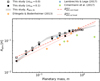Fig. 15 Comparison of the atmospheric radii obtained in our study and those in previous studies. The open and filled square symbols were obtained from our hydrodynamical simulations, ℳhw = 0 and 0.1, respectively. The gray-shaded region is given by the fitting formula for the atmospheric radius, Ratm,fit (Eq. (7)). The red dashed and dotted lines are given by Eq. (34) (Moldenhauer et al. 2022). We extrapolated Eq. (34) to the range of m ≤ 0.3. The yellow, blue, and green diamonds corresponds to the results of D’Angelo & Bodenheimer (2013), Lambrechts & Lega (2017), and Cimerman et al. (2017), respectively. To plot the results of D’Angelo & Bodenheimer (2013), the atmospheric radii were calculated by Ratm/H = CDB13a/H = CDB13/h. The values of CDB13 = 2.6 × 10−3−9.6 × 10−3 were given in Table 3 of D’Angelo & Bodenheimer (2013). We used h = max(0.027(a/1 au)1/20, 0.024 (a/1 au)2/7) (Appendix A).

5.2 Comparison to previous studies: Outflow speed

Several previous studies have proposed analytic formulae of the outflow speed, which are plotted in Fig. 9a. Ormel (2013) considered two-dimensional, isothermal, inviscid, and compressible flow past a planet. The author derived an approximate solution of the flow pattern around the planet in the linear regime in terms of the stream function: $$\Psi ={\Psi }_{\infty }+{\Psi }_{y0},$$(35)

where the first and second terms in the right-hand side of Eq. (35) correspond to the unperturbed and perturbed components. Each term can be described by $${\Psi }_{\infty }={ℳ}_{\text{hw}}x+\frac{3}{4}{x}^2,$$(36) $${\Psi }_{y0}=\frac{(\pi |y|-2y\mathrm{Si}(\tilde{y}))\cos \tilde{y}+2y\mathrm{Ci}(\tilde{y})\sin \tilde{y}}{\sqrt{2}\left|y\right|},$$(37)

where $\tilde{y}=y/\sqrt{2}$. In the right-hand side of Eq. (37), Si(y) and Ci(y) are the sine and cosine integral functions.

The flow speed in the x-direction (the radial direction to the disk) is given by υ_x,g ≈ ∂Ψ_y0/∂y in the linear regime. Ormel (2013) obtained the following formula: $${\text{υ}}_{x,\text{ out }}^{\text{O}13}=m\left[\text{Ci}(\tilde{y})\cos \tilde{y}-\frac{1}{2}(\pi -2\text{Si}(\tilde{y}))\sin \tilde{y}\right]\text{, }$$(38)

where y > 0. In a procedure of the derivation of Eq. (38), the contribution of the headwind was neglected. Equation (38) gives υ_x,g within the horseshoe region as a function of y in the shear only case (ℳ_hw = 0). In the absence of the headwind, the two-dimensional flow field has a symmetric structure with respect to the x- and y-axes. Owing to the symmetry, here we can only consider x < 0 and y > 0. Assuming that the widest horseshoe streamline can be outlined by our fitting formula (Eq. (11)), we substituted $$y=\frac{{\left(x_{\text{out }}^{-}\right)}^2}{\sqrt{{\left(w_{\text{out }}^{-}\right)}^2-{\left(x_{\text{out }}^{-}\right)}^2}}$$(39)

into Eq. (38). This gives us υ_x,g at $\left(x_{\text{out }}^{-},f_{\text{out }}\left(x_{\text{out }}^{-}\right)\right)$ on the widest inner-leading horseshoe streamline. The result was plotted in Fig. 9a with the dashed blue line.

Ormel (2013) considered the two-dimensional flow, where the three-dimensional recycling streamlines do not appear. Nevertheless, Eq. (38) agrees with our results when m ≲ 0.1 (Fig. 9a). We speculate that this comes from the close relation between the outflow region and the horseshoe streamlines. Figure 16 shows isocontours of the stream function, Ψ, and the fitting formula for the outflow region, ƒ_out(x). In Fig. 16a, where we set m = 0.03, we find that our fitting formula is in excellent agreement with the widest horseshoe streamline characterized by $\Psi ={\Psi }_{\text{HS}}=\pi m/\sqrt{2}$ (Ormel 2013). This may lead to the agreement in the results of υ_x,out between our study and Ormel (2013). The linearized approximation breaks down for the higher-mass planets. In Fig. 16b, where we set m = 0.5, we find a significant mismatch between ƒ_out(x) and Ψ. Thus, Eq. (38) does not match with υ_x,out obtained in this study when m ≳ 0.3.

Fung et al. (2015) considered isothermal and viscous flow. The authors performed three-dimensional hydrodynamical simulation for the planet with m = 0.56 and found that the outflow speed at the midplane region was ~0.2–0.4c_s. Fung et al. (2015) applied Bernoulli’s theorem along with a transient horseshoe streamline and derived the outflow speed as $$\left|{\text{υ}}_{\text{out }}^{F15}\right|=\sqrt{v_{\text{in }}^2+2m\left(\frac{1}{D_{\text{out }}}-\frac{1}{\sqrt{D_{\text{in }}^2+D_{\text{out }}^2}}\right)},$$(40)

where υ_in is the inflow speed, D_in and D_out are the distance of the inflow and outflow points from the planet. Following Fung et al. (2015), we substituted D_in ≃ H and D_out ≃ w_HS into Eq. (40), and neglected ${\upsilon }_{\text{in}}^2$. Additionally, here we assume that the outflow occurs with an angle of ~ ± π/4 to the x-axis (e.g., Fig. 8 of Fung et al. 2015). In Fig. 9a, we plotted the following modified formula for the outflow speed in the x-direction with the dashed purple line: $${\text{υ}}_{x,\text{ out }}^{\text{F}15}=\sqrt{2m\left(\frac{1}{w_{\text{HS}}}-\frac{1}{\sqrt{H^2+w_{\text{HS}}^2}}\right)}\times \cos (\pi /4).$$(41)

As discussed in Fung et al. (2015), Eq. (40) should be considered an upper limit because the height of the inflow point from the midplane assumed in Fung et al. (2015) was higher than ours. One can see that Eq. (41) overestimates the outflow speed compared to our results.

Kuwahara et al. (2019) considered isothermal and inviscid flow and performed three-dimensional hydrodynamical simulations for the planets with m = 0.01–2. Kuwahara et al. (2019) proposed that the outflow speed can be described by $$\left|{\text{υ}}_{\text{out }}^{\text{K}19}\right|=\sqrt{3R_{\text{grav }}^2}.$$(42)

Equation (42) represents the flow speed at the intersections of a line of y = −x and a circle of radius R_grav in the shear only case. Assuming that the critical recycling streamline at the midplane can be outlined by Eq. (11), we plotted the following modified formula for the x-component of the outflow speed in Fig. 9a with the dashed yellow line: $$\begin{array}{l}{\text{υ}}_{x,\text{ out }}^{\text{K}19}=\sqrt{3R_{\text{grav }}^2}\cos {\phi }_{\text{out }},\\ =\sqrt{3R_{\text{grav}}^2}\cos \left[{{\tan }^{-1}\left(\frac{\text{d}{f}_{\text{out }}(x)}{\text{d}x}\right)|}_{x=x_{\text{out }}^{K19}}\right],\end{array}$$(43)

where we assumed $x_{\text{out }}^{\text{K}19}=R_{\text{grav }}\cos (\pi /4)$ (Kuwahara et al. 2019). Equation (43) underestimates the outflow speed compared to our results for a wide range of planetary masses, m ≲ 0.3. This is caused by the following assumptions: (1) Kuwahara et al. (2019) considered an isothermal flow. (2) Kuwahara et al. (2019) set the inflow and outflow points on the sphere of radius R_grav.

In an isothermal case, there is no clear boundary demarcating the bound atmosphere from the disk gas (Ormel et al. 2015b). The inflow of the gas intrudes deep inside the gravitational sphere of the planet. Thus, in the isothermal case, the inflow and outflow points were located at the points closer to the planetary core than in the nonisothermal case, leading to an underestimation of our results. The atmospheric radius positively correlated to the cooling timescale, β, and the atmosphere disappear in the isothermal limit, β → 0 (Kurokawa & Tanigawa 2018).

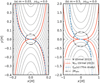Fig. 16 Isocontours of the stream function (the solid gray lines), Ψ, and the fitting formula of the critical recycling streamline at the midplane (Eq. (11); the dashed blue lines). The widest horseshoe streamlines characterized by ΨHS are highlighted with red. Isocontours of Ψ = 0.02−0.1 (panel a) and Ψ = 0.42–1.7 (panel b) are shown.

5.3 Applicability of Bernoulli’s theorem

In Sect. 3.5, assuming an isothermal flow along a recycling streamline, we estimated the outflow speed using Bernoulli’s theorem. The applicability of Bernoulli’s theorem depends on the thermodynamics of the gas along the streamline. Our hydrodynamical simulations utilized the β cooling model in which the β cooling occurs on a finite timescale. Thus, Bernoulli’s function, ℬ, does not strictly conserve along the streamline (Fig. 2c).

We begin with a qualitative discussion. When a parcel of the gas approaches the planet and reaches the region where r ≲ R_grav, the temperature of the parcel increases due to the adi-abatic compression. The temperature of the gas relaxes toward the background temperature with the dimensionless timescale β = (m/0.1)² (Eq. (5)). Assuming that the gas parcel has the shear velocity, the crossing time on which the gas crosses the gravitational sphere of the planet can be estimated by the shear timescale, τ_cross ~ Ω⁻¹. Thus, the isothermal assumption would be valid when β ≲ 1. We note that τ_cross can be longer than the shear timescale, because the gas parcel along the recycling streamline sometimes circulates the atmosphere, which leads to an increase in τ_cross (Fig. 2a).

Figures 17 and 18 show the quantitative description of Bernoulli’s function along a certain recycling streamline. Panels a and b in Figs. 17 and 18 represent the changes of ℬ and each term of ℬ as a function of y and r. Panel c of Figs. 17 and 18 shows a relative error between Bernoulli’s function and the unperturbed one, ℬ_∞. We set ${ℬ}_{\infty }={ℬ|}_{r=r_{\text{out }}}$, where ${ℬ|}_{r=r_{\text{out }}}$ corresponds to the value of ℬ at the edge of the computational domain of hydrodynamical simulations (i.e., the starting point of the streamline).

In Fig. 17, where we set m = 0.05 and β = 0.25, Bernoulli’s function is almost constant. The relative error between ℬ and ℬ_∞ is on the order of ~10⁻²−10⁻¹ and increases as the gas approaches the planet. Since the cooling time depends on the planetary mass, one would expect that the amplitude of the fluctuation of ℬ increases as the planetary mass increases. This can be seen in Fig. 18, where we set m = 0.2 and β = 4. The overall trends of Fig. 18 are similar to those of Fig. 17, but the relative error between ℬ and ℬ_∞ for m = 0.2 is ~10⁻¹−10⁰, which is larger than that for m = 0.05. We find that the relative error between ℬ and ℬ_∞ is larger for the higher-mass planets, m > 0.2 (β ≳ 10). This could lead to a mismatch between our analytic formula for the outflow speed and the numerical results in particular for a higher-mass planet (Fig. 9).

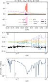Fig. 17 Quantities (panels a and b) and the relative error between ℬ and ℬ∞ (panel c) along a streamline through (x, y, z) = (0.001,0.01,0.2) (the solid colored line shown in Fig. 2c). The results were obtained from m005-hw003. Panels a and b: the solid and dotted black lines represent Bernoulli’s function, ℬ, and that in the far field, ℬ∞. The colored dashed lines correspond to the first to sixth terms in Bernoulli’s function. The dashed-dotted purple line in panel a corresponds to the x-coordinate of the streamline. The vertical solid lines in panels b and c denote twice the atmospheric radius. This figure should be compared to Fig. 2c.

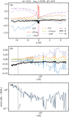Fig. 18 Same as Fig. 17, but the results were obtained from m02-003. We picked up a streamline through (x, y, z) = (0.001,0.01,0.44).

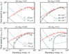Fig. 19 Same as Fig. 9, but with the terminal velocity of dust (Eq. (45); dashed-dotted blue lines). Different colors correspond to different Stokes numbers. The vertical axis is on a log scale.

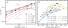Fig. 20 Atmospheric radius as a function of the planetary mass and the cooling time, β. We set ℳhw = 0. The star symbols correspond to the results obtained from the fiducial runs (Fig. 5).

5.4 Dependence on cooling time

So far we only showed the results obtained from the fiducial runs in which we considered a fixed cooling time, β₀, for a given planetary mass (Eq. (5)). To determine the β₀ value, we first considered that an inflow of a disk gas into an envelope would be heated by adiabatic compression (Sect. 2.2). We expect that the length scale of the temperature perturbation to the inflow of the disk gas can be estimated by the size of the gravitational sphere of the planet, R_Bondi or R_Hill. In this study, following Kurokawa & Tanigawa (2018), we assumed that the length scale of the temperature perturbation is equal to R_Bondi. The β₀ value represents the cooling time near the outer edge of the atmosphere. As long as we focus on the recycling flow, we consider that β₀ can be used as the typical value based on the following reasons: (1) the recycling flow traces the outer edge of the atmosphere. (2) When the dimensionless planetary mass falls below m < 0.6, which is the important mass range in this study, we always have R_grav = R_Bondi.

However, the β value could vary within the atmosphere, which becomes larger in the dense region of the atmosphere. The β value also depends on the dust opacity in the atmosphere, which could be changed by orders of magnitude (Movshovitz & Podolak 2008; Ormel 2014; Mordasini 2014). In this section, we discuss the dependence of our results on the cooling time, β. An atmospheric radius, an important quantity for gas dynamics around an embedded planet, depends on β. Qualitatively, in both the isothermal (β → 0) and adiabatic (β → ∞) limits, a bound atmosphere does not appear (Kurokawa & Tanigawa 2018; Popovas et al. 2019) or is very small (<0.2 R_Bondi; Fung et al. 2019). Figure 20 shows the dependence of the atmospheric radius on β. We find that the atmospheric radius can be scaled with the Bondi or Hill radius of the planet even when we varied β by an order of magnitude (Fig. 20a). The atmospheric radius has a peak when β ~ 1–10 (Fig. 20b). We find that R_atm is not scaled with R_Bondi or R_Hill when β = 0.01 β₀ and 100 β₀. These endmember cases approach the isothermal and adiabatic conditions, where the bound atmosphere would disappear. Thus, in the limits of β → 0 and β → ∞, there is no guarantee that R_atm will scale with R_Bondi or R_Hill.

The outflow speed in the x-direction depends on β. In Fig. 21, where we set m = 0.2, ℳ_hw = 0, and β₀ = 4, the perturbation to υ_x,g is the most prominent when β = 0.1 β₀ = 0.4. We find that the width of the horseshoe streamline would positively correlate with the atmospheric radius. Our fitting formula for the critical recycling streamline at the midplane, ƒ_out(x) (Eq. (11)), cannot be applied to the endmember cases, β ≪ β₀ and β ≫ β₀ (Fig. 21). From a series of hydrodynamical simulations, we find that ƒ_out(x) and υ_x,out (Eq. (27)) can be used when the moderate cooling time was considered, β ~ 10⁻¹−10¹. Again, the β value could be changed by orders of magnitude. Thus, further studies are needed to include the dependence of gas dynamics on the cooling time, such as the atmospheric radius, the width of the horseshoe region, and the outflow speed.

5.5 Angular momentum of the gas

Figures 17a and 18a show the changes of the x-coordinate of the gas along the recycling streamline passing outside the planetary orbit. We find that the x-coordinates of the streamline at the edges of the calculation domain of the hydrodynamical simulation do not match each other, implying that the angular momentum of the gas along the recycling streamline increases after the gravitational interaction with the planet. A detailed investigation of the net torque on the planet is beyond the scope of this study, but this result indicates that the gas flow around the planet could affect the migration rate of the planet, as suggested by Fung et al. (2015). Since our hydrodynamical simulations were performed in the local domain, our results may need to be compared with the results obtained by global hydrodynamical simulations.

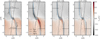Fig. 21 Same as Fig. 3, but showing the dependence of the outflow speed on the cooling time. We set m = 0.2 in all panels. The results were obtained from m02-hw0-b001 (panel a), m02-hw0-b01 (panel b), m02-hw0-b10 (panel c), and m02-hw0-b100 (panel d).

5.6 Influence of the outflow on the growth of protoplanets

Based on the analytic formula for the outflow speed (Eq. (27)), here we discuss the influence of the outflow on the growth of protoplanets. In this section, we assume that dust settle to the midplane for simplicity. More quantitatively, we assume that the vertical extent of the outflow is larger than the dust scale height. The vertical extent of the outflow can be estimated by the atmospheric radius, R_atm ≲ 0.2 H (Sect. 3.6.2). The dust scale height is given by (Youdin & Lithwick 2007) $$H_{\text{d}}={\left(1+\frac{\text{St}}{{\alpha }_{\text{diff}}}\frac{1+2\text{St}}{1+\text{St}}\right)}^{-1/2}H,$$(44)

where α_diff is the dimensionless turbulent parameter. Equation (44) gives H_d ≲ 0.3 H when St ≳ 10⁻³ and α_diff ≲ 10⁻⁴ were assumed, which means that, under weak turbulence, the outflow has a potential to affect the dust motion.

Following Kuwahara et al. (2019), we compare υ_x,out (Eq. (27)) with the terminal speed of a dust particle at a distance of r = 2 R_atm,fit from the planet, where the dominant outflow of the gas occurs. Given the force balance between the gas drag and the gravity of the planet acting on the dust particle at r = 2 R_atm,fit, the terminal speed of the dust particle can be described by $${\text{υ}}_{\text{term }}=\frac{m\text{St}}{4R_{\text{atm},\text{fit}}^2}$$(45)

in our dimensionless unit, where St is the Stokes number (the dimensionless stopping time) of dust. We plotted Eq. (45) with different Stokes numbers, St = 10⁻³ 10⁻², and 10⁻¹ in Fig. 19 and compared the terminal speed of the dust particle with the outflow speed. The outflow speed in the x-direction can exceed the terminal speed of the dust particle.

We derived the upper limit of the Stokes number of dust that can be affected by the outflow by the order-of-magnitude estimate. For simplicity, we neglected the effect of the headwind of the gas, ℳ_hw = 0, and only considered x ≥ 0. From Eqs. (27) and (45), the outflow affects the motion of dust when the Stokes number falls below the critical Stokes number: $$\text{St}\lesssim \frac{8\sqrt{3}{R}_{\text{atm},\text{fit}}^3}{m}\cos {\phi }_{\text{out }}^{+}\cos \left(\frac{2R_{\text{atm},\text{fit}}}{w_{\text{out }}^{+}}\right)\equiv {\text{St}}_{\text{crit }}.$$(46)

We plotted Eq. (46) in Fig. 22.

When m ≲ 0.1 (R_atm,fit = 0.84 R_вomdi), the product of the cosine terms in the right-hand side of Eq. (46) has ~0.6–1 and we obtain $$\text{St}\lesssim 8\sqrt{3} {\text{m}}^2\times [\text{ cos terms }]~10 {\text{m}}^2\text{. }$$(47)

When m ≳ 0.1 (R_atm,fit = 0.22 R_Hill), the product of the cosine terms in the right-hand side of Eq. (46) has ~0.3–0.6 and we obtain $$\text{St}\lesssim \frac{8\sqrt{3}}{3}\times {0.4}^3\times [\cos \text{ terms }]~\mathrm{0.1.}$$(48)

In summary, the outflow could affect the dust motion and suppress the dust accretion onto the planet when St ≲ min(10m², 0.1). This is consistent with the post-processing simulation results where the obtained hydrodynamical simulation data to calculate the dust trajectories (Kuwahara & Kurokawa 2020a,b; Okamura & Kobayashi 2021).

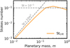Fig. 22 Upper limit of the Stokes number of dust that affected by the outflow as a function of the planetary mass (Eq. (46)).

5.7 Dust velocity influenced by the planet-induced gas flow

We expect that the analytic formulae for the distribution of the x-component of the perturbed flow velocity in the radial (υ_x,out(x); Eq. (31)) and vertical (υ_x,out(ɀ); Eq. (32)) directions to the disk can be used for modeling of the dust velocity influenced by the planet-induced gas flow. Performing hydrodynamical simulations is a direct way to investigate the influence of gas flow on dust motion, but computationally expensive. Our analytic formulae would allow us to perform an extensive parameter study of the hydrodynamic effect of the outflow on the dust motion. The above attempts at modeling dust velocity will be included in a future study.

6 Conclusions

We obtained fitting formulae that describe the morphology of gas dynamics around an embedded planet by performing three-dimensional, nonisothermal hydrodynamical simulations. We then derived an analytic formula for the planet-induced mid-plane outflow using Bernoulli’s theorem. Our main results are as follows:

• 1

  A bound atmosphere forms within the gravitational sphere of the planet, whose size scales with the Bondi or Hill radius of the planet. We derived the dimensionless fitting formula for the atmospheric radius, R_atm,fit = min(0.84 R_Bondi – 0.056 ℳ_hw, 0.36 R_Hill – 0.22 ℳ_hw). Gas from the disk chiefly flows in and out of an area of twice the atmospheric radius;

• 2

  The outflow of the gas occurs at the midplane. We find that the morphology of the outflow (the shape of the streamline) can be outlined by a simple tangential curve.

• 2

  Based on the obtained quantitative descriptions of the outflow morphology, we derived an analytic formula for the outflow speed that is in agreement with the results of hydrodynamical simulations. The outflow speed in the radial direction to the disk has a peak speed of ~0.3–0.4 c_s at m ~ 0.3, corresponding to a super-Earth mass planet at 1 au for a typical steady accretion disk model. The global pressure force of the disk gas enhances (reduces) the outflow toward the outside (inside) of the planetary orbit, causing the asymmetry of the outflow speed inside and outside the planetary orbit.

The outflow of the gas could suppress pebble accretion when St ≲ min(10m², 0.1). Our analytic formulae can be used for modeling the hydrodynamic effects of the outflow on the dust accretion onto the planet and the radial drift of dust, which could be essential for planet formation via pebble accretion and the dust ring and gap formation in a disk.

Acknowledgements

We would like to thank the reviewer, Dr. Ondrej Chrenko for thoughtful comments that have substantially improved the quality of this manuscript. We thank Athena++ developers. Numerical computations were in part carried out on Cray XC50 at the Center for Computational Astrophysics at the National Astronomical Observatory of Japan. This work was supported by JSPS KAKENHI Grant number 20KK0080, 22H01290, 22H05150, 21H04514, and 21K13976.

Appendix A Aspect ratio of the steady accretion disk

When we convert the dimensionless quantities into dimensional ones, we considered the typical steady accretion disk model with a constant turbulence strength (Shakura & Sunyaev 1973), α_acc, including viscous heating due to the accretion of the gas and irradiation heating from the central star (e.g., Ida et al. 2016). The aspect ratio of the disk is given by $$h\equiv \frac{H}{r}=\max \left(h_{\text{g},\text{vis}},h_{\text{g},\text{irr}}\right),$$(A.1)

where h_g,vis and h_g,irr are aspect ratios given by (Ida et al. 2016) $$h_{\text{g},\text{vis}}\simeq 0.027{\left(\frac{M_{*}}{1M_{\odot }}\right)}^{-7/20}{\left(\frac{{\alpha }_{\text{acc}}}{{10}^{-3}}\right)}^{-1/10}{\left(\frac{{\dot{M}}_{*}}{{10}^{-8}{M}_{\odot }/\text{yr}}\right)}^{1/5}{\left(\frac{a}{1\text{au}}\right)}^{1/20},$$(A.2) $$h_{\text{g},\text{irr}}\simeq 0.024{\left(\frac{L_{*}}{1L_{\odot }}\right)}^{1/7}{\left(\frac{M_{*}}{1M_{\odot }}\right)}^{-4/7}{\left(\frac{a}{1\text{au}}\right)}^{2/7}.$$(A.3)

In this study, we assume a solar-mass host star, M_* = 1 M_⊙, the solar luminosity, L_* = 1 L_⊙, the typical accretion rate of classical T Tauri stars, M_⊙ = 10⁻⁸ M_⊙/yr, and α_acc = 10⁻³.

Appendix B Dependence on the inner boundary

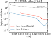Fig. B.1 Azimuthal gas velocity at the midplane averaged in the azimuthal direction in the spherical polar coordinates centered at the planet. The results were obtained from m003-hw003 and m003-hw003-01rinn. Different colors corresponds to different sizes of the inner boundary. The filled circle denotes the atmospheric radius. The dashed line shows the Keplerian speed.

In this section we investigate the influence of the size of the inner boundary (corresponding to the planet location in this study; Eq. (3)), r_inn, on the atmospheric radius. We confirmed that the size of the inner boundary does not affect our results. Previous studies reported that the azimuthal gas velocity in the spherical polar coordinates centered at the planet depends on r_inn (Ormel et al. 2015b; Béthune & Rafikov 2019; Takaoka et al. 2023). We also found that the azimuthal gas velocity varies with r_inn (Fig. B.1). Nevertheless, the atmospheric radius did not change significantly. When we changed r_inn by an order of magnitude, the relative error between the obtained atmospheric radii with r_inn = r_inn,0 and 0.1 r_inn,0 was small: ≲ 10% (Fig. B.2). This allows the orbital radius to be considered a free parameter regardless of a fixed r_inn.

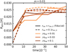Fig. B.2 Time evolution of the atmospheric radius for different sizes of the inner boundary, rinn = rinn,0 (the solid lines) and rinn = 0.1 rinn,0 (the dashed lines). Different colors correspond to different Mach numbers. We set m = 0.03 and rsm = 0.1 Rgгav.

Appendix C Dependence on the smoothing length

In this section we investigate the influence of the smoothing length on gas dynamics within the gravitational sphere of the planet, the atmospheric radius, and the outflow speed.

It is preferable to run the simulations with r_sm = 0 to resolve the local gas flow around the planet. However, through the simulations with r_sm = 0, we find unsteady and unphysical flow pattern within the atmosphere. The simulations were interrupted when we performed long-term simulations, t ≳ 500 Ω⁻¹, in particular for higher-mass planets, m ≳ 0.3. To investigate this problem, we plot the shell-averaged radial velocity in Fig. C.1. This figure show that the small but nonzero inward radial gas flow occurs at the region close to the inner boundary, meaning that the hydrostatic equilibrium is not established in this region. The density of the gas increases with time due to the continuous accumulation of the gas in the inner region of the envelope, leading to the numerical errors.

There is a clear correlation between the shell-averaged radial gas flow near the inner boundary and the smoothing length. In our parameter sets, we always have the following relation: 0.1 R_gгav < 3 r_inn. The larger the smoothing length, the smaller the radial gas velocity at the region close to the inner boundary. This can be seen in previous study and would disappear in a higher-resolution simulation (e.g., Fig. A.1 of Ormel et al. 2015b).

Figure C.2 shows the time evolution of the atmospheric radius for different smoothing lengths, r_sm = 0, 0.1 R_gгav, and 3 r_inn. In Fig. C.2a, where we set m = 0.1, we find the fluctuation of the atmospheric radius when we adopt a relatively large smoothing length, r_sm = 3 r_inn, corresponding to ~0.4 R_Bondi. The fluctuation does not occur when r_sm = 0.1 R_gгav = 0.1 R_вondi. For a higher-mass planet, m = 0.5, only when we adopt the nonzero smoothing length, the results seem to reach the steady state (Fig. C.2b).

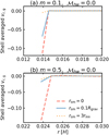Fig. C.1 Shell-averaged radial velocity of the gas in the spherical polar coordinates centered at the planet for different smoothing lengths, rsm = 0 (the dashed red line), rsm = 0.1 Rgrav (the solid blue line), and rsm = 3 rinn (the dotted yellow line). We assumed m = 0.1 in panel a and m = 0.5 in panel b. We set ℳhw = 0.

The choice of the smoothing length does not affect significantly the outflow speed when m ≲ 0.3. Figure D.1 compares the outflow speed in the x-direction obtained from hydrodynamical simulations with different smoothing lengths, r_sm = 0 and 0.1 R_grav. When m ≲ 0.3, the obtained outflow speeds are overlapped. For higher-mass planets, m ≳ 0.3, the outflow speed obtained from hydrodynamical simulations with r_sm = 0 does not match with those obtained with r_sm = 0.1 R_grav due to the unphysical flow pattern within the atmosphere.

Based on Figs. C.1–D.1, we adopt r_sm = 0.1 R_grav in our fiducial runs. It should be noted that even when we adopt the nonzero smoothing length, the inward radial gas flow does not completely disappear, indicating that the unsteady and unphysical flow pattern would eventually appear when t > 10³ Ω⁻¹.

Appendix D Interpolation of the gas velocity

We interpolated the gas velocity to plot the streamlines in the local Cartesian coordinates (e.g., the thin gray lines in Fig. 3) by using the matplotlib.pyplot.streamplot library. Our hydrodynamical simulations were performed in the spherical polar coordinates, (r, θ, ϕ), centered on the planet.

Hereafter we only consider the midplane. We set the local Cartesian coordinates, (x, y), where the following relations hold: $r=\sqrt{x^2+y^2}$ and ϕ = tan⁻¹ (y/x). We divided the local Cartesian coordinates into N grids in the x- and y-directions with equal spacing within the view range. We set N = 50. We confirmed that the result does not change significantly when we doubled the value of N. Then, we calculated the gas velocity at each Cartesian grid point with the bilinear interpolation method. The interpolated gas velocity at an arbitrary point, (x, y), is given by $$\text{υ}=(1-s)(1-t){\text{υ}}_{i,j}+s(1-t){\text{υ}}_{i+1,j}+st{\text{υ}}_{i+1,j+1}+(1-s)t{\text{υ}}_{i,j+1}\text{, }$$(D.1)

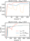Fig. C.2 Time evolution of the atmospheric radius for different smoothing lengths, rsm = 0 (the dashed red line), rsm = 0.1 Rgгav (the solid blue line), and rsm = 3 rinn (the dotted yellow line). We assumed m = 0.1 and ℳhw = 0 in panel a and m = 0.5 and ℳhw = 0 in panel b.

where υ_i,j,k is the gas velocity at the center of the grid of hydrodynamical simulations, the subscripts denote the grid number, and s and t are given by $$s=\frac{r-r_i}{r_{i+1}-r_i},$$(D.2) $$t=\frac{\varphi -{\varphi }_j}{{\varphi }_{j+1}-{\varphi }_j}.$$(D.3)

In Eqs. (D.2) and (D.3), i and j were chosen to satisfy the following relations: r_i ≤ r < r_i+1 and ϕ_j ≤ ϕ < ϕ_j+1.

The number of streamlines depends on the value of the "density" parameter in the matplotlib.pyplot.streamplot library. The default value is density=1. The number of streamlines increases as the value of the density parameter increases. To show the detailed structure of the gas flow, we set density=2 in Figs. 3, 4, and 21.

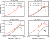Fig. D.1 Same as Fig. 9, but comparing the results obtained from hydrodynamical simulations with rsm = 0 (the cross symbols) and rsm = 0.1 Rgrav (the star symbols).

Appendix E Widest horseshoe streamline and the shear streamline passing closest to the planet

We calculated the widest horseshoe streamline and the streamline of the background shearing flow passing closest to the planet with the bisection method and plotted them in Figs. 3, 4, 7, 10, and 21 without using the matplotlib.pyplot.streamplot library. The following sections describe the dedicated calculation method for these characteristic streamlines and how to determine the boundary between the widest horseshoe streamline and the shear streamline passing closest to the planet.

Appendix E.1 Dedicated calculation method for the characteristic streamlines

This section describes the dedicated calculation method for the two characteristic streamlines: the widest horseshoe streamline and the streamline of the background shearing flow passing closest to the planet. A fifth-order Runge-Kutta-Fehlberg method was used to calculate the streamlines. We set the starting point of the streamline, (x₀, y₀), at the edge of the calculation domain of hydrodynamical simulation. The x-coordinate of the starting point, x₀, is a parameter. The y-coordinate of the starting point is given by $$y_0=\{\begin{array}{ll}\sqrt{r_{\text{out }}^2-x_0^2}\hfill & \left(x_0\ge x_{\text{cor, g}}\right),\hfill \\ -\sqrt{r_{\text{out }}^2-x_0^2}\hfill & \left(x_0<x_{\text{cor },g}\right).\hfill \end{array}$$(E.1)–(E.2)

The position of the gas parcel at the i-th time step, (x_i, y_i), was calculated by the fifth-order Runge-Kutta-Fehlberg scheme, where the gas velocity at an arbitrary position was calculated by Eq. (D.1). Following Kuwahara & Kurokawa (2020a), the maximum relative error tolerance was set to 10⁻⁸, where the authors adopted the same scheme described in this section to compute the trajectories of dust particles influenced by the planet-induced gas flow.

We terminated the above-mentioned streamline calculation when one of the following conditions was met: (1) the gas parcel reached the edge of the computational domain of hydrodynamical simulations, $\sqrt{x_i^2+y_i^2}\ge r_{\text{out}}(i=1,2,\dots )$, or (2) the gas parcel reached a stagnation point. We judged that a parcel of the gas reached the stagnation point when $$\frac{\left|{\text{υ}}^{i+1}-{\text{υ}}^i\right|}{\delta t}\le ϵ.$$(E.3)

In Eq. (E.3), $v^i=\sqrt{v_{x,i}^2+v_{y,i}^2}$ is the gas speed at (x_i, y_i) where the x- and y-components of the gas velocity, υ_x,i and υ_y,i are calculated by Eq. (D.1) and we set ϵ = 10⁻¹⁰.

Appendix E.2 Determination of the boundary between the widest horseshoe streamline and the shear streamline passing closest to the planet

Based on the dedicated calculation method for the characteristic streamlines described in Appendix E.1, we determined the boundary between the widest horseshoe streamline and the shear streamline passing closest to the planet with the bisection method. We calculated the streamlines with the initial spatial intervals of δx₀ = 10⁻² H in the x-direction. We denote with $x_0^j$ and $x_{\text{e}}^j$ the x-coordinates of the starting and end points of the j-th streamline, respectively. We classified the obtained streamline as a horseshoe streamline when $x_{\text{e}}^j<x_{\text{cor,g}}$ and $x_0^j>x_{\text{cor,g}}$, or $x_{\text{e}}^j>x_{\text{cor,g}}$ and $x_0^j<x_{\text{cor,g}}$, where $x_{\text{e }}^j$ is the x -coordinate of the j-th streamline at the edge of the computational domain of hydrodynamical simulation; otherwise, it was classified as a shear streamline.

When the j-th and (j + 1)-th streamlines were determined to be the shear and horseshoe streamlines, respectively, we set $x_0^j\equiv a_0,x_0^{j+1}\equiv b_0$, and c₀ ≡ (a₀ + b₀)/2. We calculated a streamline whose x-coordinate of the starting point was c₀, and then set a₁ ≡ c₀, b₁ ≡ b₀ (b₁ ≡ c₀, a₁ ≡ a₀), and c₁ ≡ (a₁ + b₁)/2 when the streamline was determined to be a shear (horseshoe) streamline. We repeated the above steps until the following condition was satisfied: |a_k − b_k| < 0.01 δx₀ = 10⁻⁴ H (k = 0, 1,…).

Appendix F Numerical convergence

To obtain the atmospheric radius, we used the final state of the hydro-simulations data (Sect. 3.1). Figure F.1 shows the time evolution of the atmospheric radius for different planetary masses, m = 0.05, 0.1, 0.2, and 0.5, and Mach numbers, ℳ_hw = 0−0.1. We set r_sm = 0.1 R_grav. The atmospheric radius increases in the early stage of the time evolution and reaches a steady state after t ≳ 30−100 Ω⁻¹.

Appendix G Numerically calculated widths of the horseshoe and outflow regions

Based on the streamline calculation method described in Appendix E, we calculated numerically the x-coordinate of the critical recycling streamline at the midplane, $x_{\text{rec,num}}^{\pm }$, and the half-width of the horseshoe region, $w_{\text{HS,num}}^{\pm }$. We defined $x_{\text{rec,num}}^{\pm }$ as the x-coordinate of the shear streamline passing closest to the planet at the edge of the computational domain of our hydrodynamical simulations. We defined the numerically calculated half-width of the horseshoe flow as $$w_{\text{HS},\text{ num }}^{+}=x_{\text{OL},\text{HS}}^{\text{num }}+\left|x_{\text{cor},\text{g}}\right|,$$(G.1) $$w_{\text{HS},\text{ num }}^{-}=\left|x_{\text{IT},\text{HS}}^{\text{num }}\right|-\left|x_{\text{cor,g }}\right|,$$(G.2)

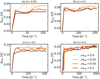Fig. F.1 Time evolution of the atmospheric radius for different planetary masses, m = 0.05 (panel a), m = 0.1 (panel b), m = 0.2 (panel c), and m = 0.5 (panel d). Different colors correspond to different Mach numbers. We set rsm = 0.1 Rgrav in this figure.

where $x_{\text{OL},\text{HS}}^{\text{num}}$ and $x_{\text{IT},\text{HS}}^{\text{num}}$ are the x-coordinates of the widest outer-leading and inner-trailing horseshoe flows at the edges of the computational domain of our hydrodynamical simulations (the starting points of the streamlines in the first and third quadrants in the x-y plane).

Figure G.1 compares the numerically calculated quantities, $x_{\text{rec,num}}^{\pm }$ and $w_{\text{HS},\text{num}}^{\pm }$, with the analytic formulae. We find that $w_{\text{HS}}^{\text{JM17}}$ (Eq. (15)) is a better indicator than $w_{\text{HS}}^{\text{MB16}}$ (Eq. (14)) in describing the width of the outflow region when m ≲ 0.6, though a mismatch between the numerical results and the analytic estimate is prominent when m ~ 0.2 (the circle symbols and the solid lines in Fig. G.1).

Since our analytic model for the gas flow is not valid in the higher-mass regime (m ≳ m_iso ≃ 0.6; see Sect. 3.2.1), here we restrict our attention to the limited range of the planetary mass, m < 0.6. We speculate that the significant deviation between $x_{\text{rec},\text{num}}^{\pm }$ and $w_{\text{HS}}^{\text{JM}17}$ around m ~ 0.2 is related to the dependence of υ_x,out on the planetary mass. As shown Fig. 9, υ_x,out has a peak when m ~ 0.3, which means that a parcel of the gas moves significantly in the x-direction and $x_{\text{rec},\text{num}}^{\pm }$ increases. The deviation between $x_{\text{rec},\text{num}}^{\pm }$ and the analytic estimate around m ~ 0.2 is likely caused by the existence of the recycling flow revealed by our local three-dimensional hydrodynamical simulations, which have a higher resolution within the gravitational sphere of the planet, R_grav.

The influence of the recycling flow may not be included in both Eqs. (14) and (15). Equation (15) was based on Eq. (14), and Eq. (14) was derived by a combination of linear theory and the results of three-dimensional global hydrodynamical simulations with the moderate resolution at ≲ R_grav (Masset & Benítez-Llambay 2016). Nevertheless, we keep ourselves conservative for the estimation of x_rec and assume that Eq. (15) is valid in deriving the width of the outflow region.

While the width of the outflow region is better described by $w_{\text{HS}}^{\text{JM}17}$ (Eq. (15)), we find that the half-width of the horseshoe flow agrees with $w_{\text{HS}}^{\text{MB}17}$ (Eq. (14)) regardless of the assumed Mach number of the headwind, except when m < 0.1 (the square symbols and the dotted lines in Fig. G.1). When m < 0.1, the horseshoe region might not be well established in our hydrodynamical simulations.

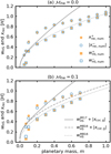Fig. G.1 Width of the horseshoe flow and the x-coordinate of the critical recycling streamline at the edge of the computational domain of hydrodynamical simulations. The solid, dotted, and dashed gray lines are given by the analytic formulae for the width of the horseshoe region (Eqs. (14) and (15)). The numerically calculated width of the outflow region (xrec,num, the circle symbols) is in better agreement with the analytic estimate based on Eq. (15) ($w_{\text{HS}}^{\text{JB}17}$, the solid lines) than Eq. (14) (the dashed line). The numerically calculated width of the horseshoe region (wHS,num, the squares symbols) is in good agreement with Eq. (14) ($w_{\text{HS}}^{\text{MB}16}$, the dotted lines).

Although a discrepancy between $w_{\text{HS},\text{num}}^{\pm }$ and $w_{\text{HS}}^{\text{JM}17}$ (Eq. (15)) does not affect an analytic derivation of the outflow speed, we discuss the reason of this discrepancy below. The discrepancy between $w_{\text{HS,num}}^{\pm }$ and $w_{\text{HS}}^{\text{JM}17}$ (Eq. (15)) could be caused by the limitation of our hydrodynamical simulations. Our local simulation cannot handle the gas-gap opening in the high-mass regime, m ≳ m_iso. Gas-gap formation reduces the Lindblad torque, leading to an extension of the horseshoe region into the Lindblad resonance region, ~H (Paardekooper & Papaloizou 2009). Then the dependence of the horseshoe width on the planetary mass deviates from $w_{\text{HS}}^{\text{MB}16}\propto \sqrt{m}$. Moreover, our local hydrodynamical simulations were performed on the spherical polar coordinates with a logarithmic grid for the radial coordinate, which has a lower resolution at the region far from the planet. We fixed the gas velocity at the outer edge of the computational domain of hydrodynamical simulations. These simulation settings could affect the width of the horseshoe flow.

References

All Tables

All Figures

Fig. 1 Planetary mass (top) and the Mach number (bottom) as a function of the orbital radius. For the conversion, we assumed a typical steady accretion disk model with a dimensionless viscous alpha parameter (Shakura & Sunyaev 1973), αacc, including viscous heating and stellar irradiation (e.g., Ida et al. 2016). In this model, the aspect ratio is given by h = max(0.027(a/1 au)1/20, 0.024 (a/1 au)2/7), where a solar-mass star, a solar luminosity, the typical accretion rate of classical T Tauri stars, 10−8 M⊙ yr−1, and αacc = 10−3 were assumed (Appendix A).

In the text

Fig. 2 Streamlines of gas flow around the planet with m = 0.05 and ℳhw = 0.03. The arrows represent the direction of the gas flow. Panel a: perspective view of the flow field. Different colors correspond to different types of streamlines. The size of the atmosphere is 0.04 H. Panel b: same as panel a, but the color contour represents p/ρg, which is the measure of temperature (Sect. 3.3). Panel c: x-y plane viewed from the +z-direction. The critical streamline is highlighted by the color contour, which represents Bernoulli’s function, ℬ (Sects. 3.3 and 5.3).

In the text

Fig. 3 Dependence of the planet-induced gas flow on the planetary mass at the midplane. We set ℳhw = 0 in all panels. The results were obtained from m005-hw0 (panel a), m01-hw0 (panel b), m05-hw0 (panel c), and m07-hw0 (panel d). The solid thin gray lines are gas streamlines. The solid and thick dashed gray lines are the widest horseshoe streamline and the shear streamline passing closest to the planet, respectively (Appendix E). The color contour represents the flow speed in the x-direction. The dashed and dashed-dotted black circles denote the atmospheric radius (Eq. (5)) and twice the atmospheric radius, where the outflow speed is measured. The dashed blue lines are the curves representing the fitting formula for the critical recycling streamline (Eq. (11); Sect. 3.2.1). The vertical lines are the asymptotes of Eq. (11), representing the extent of the outflow region in the x-direction ((Eq. (17)); Sect. 3.2.2). The horizontal lines denote the y-coordinates of the characteristic length of the outflow region in the y-direction ((Eq. (18)); Sect. 3.2.3).

In the text

	Fig. 4 Same as Fig. 3, but showing the dependence of the planet-induced gas flow on the Mach number of the headwind. We set m = 0.2 in all panels. The results were obtained from m02-hw0 (panel a), m02-hw001 (panel b), m02-hw003 (panel c), and m02-hw01 (panel d). The vertical dotted line corresponds to the corotation radius for the gas.
In the text

	Fig. 5 Atmospheric radius as a function of the planetary mass and the Mach number of the headwind of the gas. The square symbols were obtained from hydrodynamical simulations. Different colors correspond to different Mach numbers, ℳhw. The gray-shaded region is given by the fitting formula for the atmospheric radius, Ratm,fit. The dashed gray line is given by Eq. (9).
In the text

Fig. 6 Shell-averaged values of $p/{\rho }_{\text{g}}^{\gamma }$ (panel a) and p/ρg (panel b), which are the measures of the entropy and the temperature, respectively, as a function of the distance from the planet. We set γ = 1.4. Different colors correspond to different planetary masses. The filled circles, the squares, and the triangles denote the atmospheric radius, the Bondi radius, and the Hill radius, respectively. We set ℳhw = 0.

In the text

Fig. 7 Difference of the flow speed from the unperturbed Keplerian shear. The results were obtained from m01 − hw0 (panel a) and m05 − hw0 (panel b). The dashed blue, dashed-dotted white, and dotted white lines denote the fitting formula for the critical recycling streamline, the x-coordinate of the critical recycling streamline at the midplane in the far field, and the x-coordinate of the edge of the subsonic region, respectively. As in Fig. 3, we highlight the widest horseshoe streamline and the shear streamline passing closest to the planet with the solid and dashed orange lines, respectively.

In the text

Fig. 8 Gas flow structure and azimuthally averaged mass flux. The results were obtained from m02 − hw0 (panels a and b), m02 − hw01 (panels c and d), and m04 − hw0 (panels e and f). Left column: gas flow structure at the meridian plane. The color contour represents the r-component of the gas velocity in the spherical polar coordinates centered at the planet and averaged in the y-direction within the calculation domain of the hydrodynamical simulation. The dashed, dotted, and dashed-dotted circles denote the Bondi radius, the Hill radius, and twice the atmospheric radius, respectively. Right column: mass flux of the gas averaged in the azimuthal direction in the spherical polar coordinates centered at the planet, 〈ρgυr〉ϕ. Each solid line represents the changes in 〈ρgυr〉ϕ; altitude is varied along with a certain radius. We highlight the important radii with solid yellow (RBondi), blue (RHill), and red (2 Ratm) lines.

In the text

Fig. 9 Outflow speed at the midplane as a function of the dimensionless planetary mass and the Mach number of the headwind of the gas. The star symbols were obtained from hydrodynamical simulations, corresponding to the maximum flow speeds in the x-direction toward the outside (red) and inside (black) of the planetary orbit within the limited region, $w_{\text{out }}^{-}\le x\le w_{\text{out }}^{+},L_{\text{out }}^{-}\le y\le L_{\text{out }}^{+}$, and $\sqrt{x^2+y^2}\ge R_{\text{atm }}$. The last condition avoids incorrectly sampling the large υx,g within the atmosphere. The solid red and black lines correspond to the analytic formulae for the x-components of the outflow speeds (Eq. (27)). The dashed lines correspond to the analytic formulae for the outflow speed in the x-direction obtained by Ormel (2013, blue; Eq. (38)), Fung et al. (2015, purple; Eq. (41)), and Kuwahara et al. (2019, yellow; Eq. (43)). The gray shading marks the region where the planetary mass exceeds the pebble isolation mass, miso (Eq. (12)).

In the text

References

- Ataiee, S., Baruteau, C., Alibert, Y., & Benz, W. 2018, A&A, 615, A110 [NASA ADS] [CrossRef] [EDP Sciences] [Google Scholar]
- Bailey, A., Stone, J. M., & Fung, J. 2021, ApJ, 915, 113 [NASA ADS] [CrossRef] [Google Scholar]
- Béthune, W., & Rafikov, R. R. 2019, MNRAS, 488, 2365 [Google Scholar]
- Bitsch, B., Morbidelli, A., Johansen, A., et al. 2018, A&A, 612, A30 [NASA ADS] [CrossRef] [EDP Sciences] [Google Scholar]
- Chrenko, O., & Lambrechts, M. 2019, A&A, 626, A109 [NASA ADS] [CrossRef] [EDP Sciences] [Google Scholar]
- Cimerman, N. P., Kuiper, R., & Ormel, C. W. 2017, MNRAS, 471, 4662 [Google Scholar]
- D’Angelo, G., & Bodenheimer, P. 2013, ApJ, 778, 77 [Google Scholar]
- D’Angelo, G., & Lubow, S. H. 2008, ApJ, 685, 560 [CrossRef] [Google Scholar]
- Duffell, P. C., & MacFadyen, A. I. 2013, ApJ, 769, 41 [NASA ADS] [CrossRef] [Google Scholar]
- Eggleton, P. P. 1983, ApJ, 268, 368 [Google Scholar]
- Fung, J., Artymowicz, P., & Wu, Y. 2015, ApJ, 811, 101 [Google Scholar]
- Fung, J., Zhu, Z., & Chiang, E. 2019, ApJ, 887, 152 [NASA ADS] [CrossRef] [Google Scholar]
- Gammie, C. F. 2001, ApJ, 553, 174 [Google Scholar]
- Goodman, J., & Rafikov, R. 2001, ApJ, 552, 793 [NASA ADS] [CrossRef] [Google Scholar]
- Ida, S., Guillot, T., & Morbidelli, A. 2016, A&A, 591, A72 [NASA ADS] [CrossRef] [EDP Sciences] [Google Scholar]
- Jiménez, M. A., & Masset, F. S. 2017, MNRAS, 471, 4917 [Google Scholar]
- Kurokawa, H., & Tanigawa, T. 2018, MNRAS, 479, 635 [Google Scholar]
- Kuwahara, A., & Kurokawa, H. 2020a, A&A, 633, A81 [NASA ADS] [CrossRef] [EDP Sciences] [Google Scholar]
- Kuwahara, A., & Kurokawa, H. 2020b, A&A, 643, A21 [NASA ADS] [CrossRef] [EDP Sciences] [Google Scholar]
- Kuwahara, A., Kurokawa, H., & Ida, S. 2019, A&A, 623, A179 [NASA ADS] [CrossRef] [EDP Sciences] [Google Scholar]
- Kuwahara, A., Kurokawa, H., Tanigawa, T., & Ida, S. 2022, A&A, 665, A122 [NASA ADS] [CrossRef] [EDP Sciences] [Google Scholar]
- Lambrechts, M., & Lega, E. 2017, A&A, 606, A146 [NASA ADS] [CrossRef] [EDP Sciences] [Google Scholar]
- Lambrechts, M., Johansen, A., & Morbidelli, A. 2014, A&A, 572, A35 [NASA ADS] [CrossRef] [EDP Sciences] [Google Scholar]
- Masset, F. S., & Benítez-Llambay, P. 2016, ApJ, 817, 19 [NASA ADS] [CrossRef] [Google Scholar]
- Masset, F. S., D’Angelo, G., & Kley, W. 2006, ApJ, 652, 730 [NASA ADS] [CrossRef] [Google Scholar]
- Moldenhauer, T., Kuiper, R., Kley, W., & Ormel, C. 2021, A&A, 646, A11 [NASA ADS] [CrossRef] [EDP Sciences] [Google Scholar]
- Moldenhauer, T., Kuiper, R., Kley, W., & Ormel, C. 2022, A&A, 661, A142 [NASA ADS] [CrossRef] [EDP Sciences] [Google Scholar]
- Mordasini, C. 2014, A&A, 572, A118 [NASA ADS] [CrossRef] [EDP Sciences] [Google Scholar]
- Movshovitz, N., & Podolak, M. 2008, Icarus, 194, 368 [NASA ADS] [CrossRef] [Google Scholar]
- Nakagawa, Y., Sekiya, M., & Hayashi, C. 1986, Icarus, 67, 375 [Google Scholar]
- Okamura, T., & Kobayashi, H. 2021, ApJ, 916, 109 [NASA ADS] [CrossRef] [Google Scholar]
- Ormel, C. W. 2013, MNRAS, 428, 3526 [NASA ADS] [CrossRef] [Google Scholar]
- Ormel, C. W. 2014, ApJ, 789, L18 [Google Scholar]
- Ormel, C. W., Kuiper, R., & Shi, J.-M. 2015a, MNRAS, 446, 1026 [NASA ADS] [CrossRef] [Google Scholar]
- Ormel, C. W., Shi, J.-M., & Kuiper, R. 2015b, MNRAS, 447, 3512 [Google Scholar]
- Paardekooper, S.-J., & Mellema, G. 2004, A&A, 425, L9 [NASA ADS] [CrossRef] [EDP Sciences] [Google Scholar]
- Paardekooper, S.-J., & Papaloizou, J. 2009, MNRAS, 394, 2297 [NASA ADS] [CrossRef] [Google Scholar]
- Paczynski, B. 1971, ARA&A, 9, 183 [NASA ADS] [CrossRef] [Google Scholar]
- Popovas, A., Nordlund, Å., Ramsey, J. P., & Ormel, C. W. 2018, MNRAS, 479, 5136 [Google Scholar]
- Popovas, A., Nordlund, Å., & Ramsey, J. P. 2019, MNRAS, 482, L107 [NASA ADS] [CrossRef] [Google Scholar]
- Shakura, N. I., & Sunyaev, R. A. 1973, A&A, 24, 337 [NASA ADS] [Google Scholar]
- Stone, J. M., Tomida, K., White, C. J., & Felker, K. G. 2020, ApJS, 249, 4 [NASA ADS] [CrossRef] [Google Scholar]
- Takaoka, K., Kuwahara, A., Ida, S., & Kurokawa, H. 2023, A&A, 674, A193 [NASA ADS] [CrossRef] [EDP Sciences] [Google Scholar]
- White, C. J., Stone, J. M., & Gammie, C. F. 2016, ApJ, 225, 22 [NASA ADS] [Google Scholar]
- Youdin, A. N., & Lithwick, Y. 2007, Icarus, 192, 588 [NASA ADS] [CrossRef] [Google Scholar]
Precisely, the mass range is dependent on parameters such as the orbital radius; see Sect. 2.
This flow is also referred to as the transient horseshoe flow in Fung et al. (2015).