| Issue |
A&A
Volume 663, July 2022
|
|
|---|---|---|
| Article Number | A37 | |
| Number of page(s) | 16 | |
| Section | Interstellar and circumstellar matter | |
| DOI | https://doi.org/10.1051/0004-6361/202142453 | |
| Published online | 08 July 2022 | |
First look at the multiphase interstellar medium using synthetic observations from low-frequency Faraday tomography
1
Ruđer Bošković Institute,
Bijenička cesta 54,
10000
Zagreb, Croatia
e-mail: This email address is being protected from spambots. You need JavaScript enabled to view it.
2
Laboratoire AIM, CEA/CNRS/Université Paris-Saclay,
91191
Gif-sur-Yvette, France
3
Scuola Normale Superiore,
Piazza dei Cavalieri, 7
56126
Pisa, Italy
4
Institute of Astrophysics, Foundation for Research and Technology-Hellas,
Vasilika Vouton,
GR-70013
Heraklion, Greece
5
INAF – Osservatorio Astrofísico di Arcetri,
Largo E. Fermi 5,
50125
Firenze, Italy
6
ASTRON, the Netherlands Institute for Radio Astronomy,
Oude Hoogeveensedijk 4, 7991
PD
Dwingeloo, The Netherlands
7
Kapteyn Astronomical Institute, University of Groningen,
PO Box 800,
9700 AV
Groningen, The Netherlands
Received:
15
October
2021
Accepted:
14
April
2022
Abstract
Faraday tomography of radio polarimetric data below 200 MHz from the LOw Frequency ARray (LOFAR) has been providing new perspectives on the diffuse and magnetized interstellar medium (ISM). One aspect of particular interest is the unexpected discovery of Faraday-rotated synchrotron polarization associated with structures of neutral gas, as traced by atomic hydrogen (HI) and dust. Here, we present the first in-depth numerical study of these LOFAR results. We produced and analyzed comprehensive synthetic observations of low-frequency synchrotron polarization from magneto-hydrodynamical (MHD) simulations of colliding super shells in the multiphase ISM from the literature. Using an analytical approach to derive the ionization state of the multiphase gas, we defined five distinct gas phases over more than four orders of magnitude in gas temperature and density, ranging from hot, and warm fully ionized gas to a cold neutral medium. We focused on establishing the contribution of each gas phase to synthetic observations of both rotation measure and synchrotron polarized intensity below 200 MHz. We also investigated the link between the latter and synthetic observations of optically thin HI gas. We find that it is not only the fully ionized gas, but also the warm partially ionized and neutral phases that strongly contribute to the total rotation measure and polarized intensity. However, the contribution of each phase to the observables strongly depends on the choice of the integration axis and the orientation of the mean magnetic field with respect to the shell collision axis. A strong correlation between the HI synthetic data and synchrotron polarized intensity, reminiscent of the LOFAR results, is obtained with lines of sight perpendicular to the mean magnetic field direction. Our study suggests that multiphase modeling of MHD processes is needed in order to interpret observations of the radio sky at low frequencies. This work is a first step toward understanding the complexity of low-frequency synchrotron emission that will be soon revolutionized thanks to large-scale surveys with LOFAR and the Square Kilometre Array.
Key words: ISM: magnetic fields / ISM: structure / ISM: bubbles / methods: numerical / polarization / radio continuum: ISM
© A. Bracco et al. 2022
 Open Access article, published by EDP Sciences, under the terms of the Creative Commons Attribution License (https://creativecommons.org/licenses/by/4.0), which permits unrestricted use, distribution, and reproduction in any medium, provided the original work is properly cited.
This article is published in open access under the Subscribe-to-Open model. This email address is being protected from spambots. You need JavaScript enabled to view it. to support open access publication.
1 Introduction
Magnetic fields are fundamental ingredients of the turbulent cascade that steers and shapes the diffuse interstellar gas from kiloparsec to sub-parsec scales where star formation occurs (see e.g., the review by Hennebelle & Inutsuka 2019). However, the interaction of magnetic fields with interstellar matter is very difficult to characterize observationally. One reason for this difficulty is that this interaction is not only multiscale, but multiphase as well. Depending on the thermodynamics of interstellar gas a number of distinct phases can be identified based on observations (Heiles & Haverkorn 2012; Ferrière 2020). Fully ionized gas is at temperatures above 106 K (hot ionized medium, HIM) or at ~104 K (warm ionized medium, WIM), based on X-ray, UV, and optical spectroscopy (e.g., Snowden et al. 1997; Jenkins 2013; Krishnarao et al. 2017). In addition, UV spectroscopy of the local ISM has also suggested the presence of gas at lower temperatures (~5000 K) with ionization fraction of about 0.5 (warm partially ionized medium, WPIM, Fitzpatrick & Spitzer 1997; Redfield & Linsky 2004). The mostly neutral phases in the diffuse ISM (with ionization fractions below 10−2) are well-known through line emission of atomic hydrogen (HI) at 21 cm. The HI gas is a mixture of bi-stable gas composed of warm neutral medium (WNM), at temperatures of ~8000 K, and a cold neutral medium (CNM), with corresponding temperature of ~50 K (Field 1965; Wolfire et al. 2003). As it is subject to thermal instability, HI gas also contains an unstable, lukewarm, neutral medium (LNM), which can be considered an intermediate phase between the two stable phases (e.g., Saury et al. 2014; Marchal et al. 2019).
Synchrotron emission and polarization are the main observational probes of interstellar magnetic fields (Haslam et al. 1982; Reich & Reich 1986; Davies et al. 1996; Guzmán et al. 2011; Mozdzen et al. 2017, 2019; Beck et al. 2019). Therefore, if we want to understand magneto-hydrodynamical (MHD) turbulence in the ISM, we need to correctly interpret the synchrotron data. Polarimetric observations of the LOw Frequency ARray (LOFAR, van Haarlem et al. 2013) below 200 MHz recently started set into question our understanding of how synchrotron emission propagates throughout the diffuse and magnetized ISM. In particular, diffuse synchrotron emission is not expected to be specifically related to any gas phase listed above. It is the result of the interaction of cosmic ray electrons (CRe) and magnetic fields that are ubiquitous in the diffuse ISM (Padovani & Galli 2018). However, in a number of studies, LOFAR observations revealed a striking morphological correlation between the structure of the observed synchrotron polarization and structures of neutral ISM, both traced by HI emission (Kalberla & Kerp 2016; Jelić et al. 2018; Bracco et al. 2020; Turić et al. 2021) and interstellar dust (Zaroubi et al. 2015; Van Eck et al. 2017; Turić et al. 2021).
Below 1 GHz, Faraday rotation complicates the interpretation of these observations (i.e., Beck 2015). Magnetic fields and thermal electrons in the ionized multiphase gas along the line of sight (LOS) Faraday rotate the diffuse synchrotron polarized emission. The observed link between LOFAR polarization and neutral phases must be related to the full complexity of the magneto-ionic ISM, where synchrotron emission and Faraday rotation are mixed. A powerful technique used to disentangle various contributions of magneto-ionic medium along the LOS is called Faraday tomography (Burn 1966; Brentjens & de Bruyn 2005). This technique takes radio-polarimetric data and decomposes the observed polarized synchrotron emission by the amount of Faraday rotation that it experiences along the LOS. Faraday tomography maps the 3D relative distribution of the intervening magneto-ionic ISM based on Faraday depth. This quantity represents the specific amount of rotation measure along the LOS, which is the integrated effect of magnetic fields and thermal-electron density.
In light of Faraday tomography, which is sensitive to ionized gas, the correlation with the neutral phases revealed by LOFAR data is even more interesting. The question that arises is whether LOFAR is able to detect small amounts of Faraday depth coming from neutral clouds (as discussed in Bracco et al. 2020) or whether LOFAR is directly sensitive to synchrotron polarization associated to WNM, LNM, and CNM (as first suggested by Van Eck et al. 2017). This latter hypothesis would imply that Faraday rotation in the ionized gas fully depolarizes synchrotron emission in the WIM and in the HIM, highlighting synchrotron polarization from the neutral phases. Any of the two scenarios suggests that LOFAR is providing us with a completely new perspective on the diffuse ISM.
In order to investigate in depth these observations and study the complex, non-linear dependencies of synchrotron emission with the multiphase and magnetized ISM, a thorough analysis of MHD numerical simulations is needed. Synthetic observations of Faraday tomography from MHD numerical simulations have been already presented in recent works (Basu et al. 2019; Seta & Federrath 2021). However, to our knowledge, the multiphase aspect of the problem has never been addressed before.
Hence, we present the first synthetic low-frequency radio polarimetric observations of MHD simulations of a multiphase ISM. Since shells and loops are typical features observed in synchrotron emission (e.g., Berkhuijsen 1971; Vidal et al. 2015; Panopoulou et al. 2021; Erceg et al. 2022), we have chosen to analyze synthetic observations of Faraday tomography at LOFAR frequencies from simulations of two colliding super shells presented in Ntormousi et al. (2017). Our effort is only a first step in understanding the diffuse radio emission at low frequencies as a function of the ionization state of the ISM. A better knowledge of the diffuse synchrotron emission of the Galaxy will be crucial for interpreting the upcoming large-scale surveys from LOFAR (e.g., the LOFAR two-meter Sky Survey – LoTSS, Shimwell et al. 2017) and the Square Kilometre Array in the future (Dewdney et al. 2009).
The paper is organized as follows. In Sect. 2, we describe the methodology used to model synchrotron emission and polarization below 200 MHz. We also present the MHD simulations and detail how we estimated the ionization state of the multiphase gas. Section 3 presents our main results, which include: maps of rotation measure (Sect. 3.1); the distinct contribution of magnetic fields and electrons to the rotation measure (Sect. 3.2); and the correlation of the multiphase gas both with rotation measure (Sect. 3.3) and with polarized intensity based on Faraday tomography (Sects. 3.4 and 3.5). These results are discussed in Sect. 4, while Sect. 5 presents our summary and conclusion. The manuscript includes two appendices.
2 Methods
In this section, we describe the methodology and formalism for the purpose of modeling intrinsic1 synchrotron emission (Sect. 2.1), Faraday rotation and synthetic Faraday cubes (based on Faraday tomography, Sect. 2.2) from the MHD simulations presented in Sect. 2.3. For more details on Faraday tomography, please refer to Burn (1966), Brentjens & de Bruyn (2005), and Ferrière (2020).
We modeled the total synchrotron emission at frequency, v, by producing synthetic observations of Stokes Iv, while we model the corresponding linear polarization by synthetic observations of Stokes Qv and Uv. Because of the Faraday rotation angle’s proportionality to the λ2, modeling it accurately is crucial for observations below 200 MHz. This would not be necessary for models of synchrotron emission at higher radio frequencies (>10GHz).
The methodology described in Sects. 2.1 and 2.2 is general and can be applied to any MHD simulation that provides magnetic field  2 and an estimate of the number density of thermal electrons, ne, in 3D.
2.1 Intrinsic synchrotron emissivity
We modeled intrinsic synchrotron total and polarized emission following Padovani et al. (2021, hereafter P21). As CRe propagate through the ISM, they lose energy via a number of mechanisms that involve interactions with matter, magnetic fields, and radiation (Longair 2011). These processes deplete the population of CRe and change their original energy spectrum, je(E)3, where E is the energy of the CRe. Obtaining an accurate model for je(E) is important as it determines the amount of specific emissivity of intrinsic synchrotron emission at frequency, v. The specific emissivity can be split into two components linearly polarized along and across the component of the magnetic field perpendicular to the LOS, B⊥, as follows
 (1)
(1)
In Eq. (1), υe is the electron velocity, me is the electron mass, c is the speed of light,  are the power per unit frequency emitted by an electron of energy, E, at frequency, v, for the two polarizations, and B⊥ is the strength of B⊥ at position r. For more details on Eq. (1), we refer to P21, Ginzburg & Syrovatskii (1964), and Rybicki & Lightman (1979).
The main difference of the P21 approach compared to previous works is that it includes realistic observational constraints on je(E), set by considering the energy dependence of the spectral energy slope (e.g., Sun et al. 2008; Waelkens et al. 2009; Reissl et al. 2019; Wang et al. 2020). Following P21, in our models we consider a uniform spatial distribution of CRe and we use the je(E) from Orlando (2018). This CRe energy spectrum is based on multifrequency observations, from radio to γ-rays, as well as Voyager-1 measurements, and it is representative of most of the local radio synchrotron emission within ~ 1 kpc from the Sun. The use of a data-driven dependence of je(E) with E, as discussed in P21, is particularly relevant at low radio frequencies. Standard approaches that consider a single power-law slope, of the kind je ∝ Es with s = −2 or −3 depending on the energy range of the CRe (e.g., Sun et al. 2008; Waelkens et al. 2009; Wang et al. 2020), strongly bias the estimate of the synchrotron emissivities in the diffuse ISM toward flatter synchrotron spectral energy distributions (see P21 for more details).
We build synthetic maps of the total synchrotron emission, Stokes Iv, by integrating the quantity εv,‖(r) + εv,⊥(r) along any given LOS of the simulated cubes.
2.2 Faraday rotation and synthetic Faraday cubes
In polarization, the derivation of the Stokes Qv and Uv maps is more complicated in the presence of Faraday rotation. In this work, we consider the case where Faraday rotation is fully mixed with synchrotron emission, giving rise to differential Faraday rotation (e.g., Sokoloff et al. 1998). Each slice in the simulated cubes contributes both to synchrotron emission and Faraday rotation. This means that the synthetic synchrotron Stokes Qv and Uv are not only the result of integrating the corresponding emissivities along the LOS (as in P21), neglecting the effect of Faraday rotation. Instead, we introduced effective synchrotron emissivities in polarization,  and
and  , by modifying Eqs. (6) and (7) in P21 and defining the specific polarized emissivity at the i-th slice along a given LOS r as:
 (2)
(2)
Given Eq. (2), in the limit of small-size voxels compared to the simulation cube, we compute  at the ith slice as
![Mathematical equation: ${\tilde \varepsilon _{v,Q}}\left( {{{\bf{r}}_i}} \right) = {\varepsilon _{v,P}}\left( {{{\bf{r}}_i}} \right)\,\cos \,2\,\left[ {\varphi \left( {{{\bf{r}}_i}} \right) + \delta R{M_i}{{\left( {{c \over v}} \right)}^2}} \right],$](/articles/aa/full_html/2022/07/aa42453-21/aa42453-21-eq8.png) (3)
(3)
and
![Mathematical equation: ${\tilde \varepsilon _{v,U}}\left( {{{\bf{r}}_i}} \right) = {\varepsilon _{v,P}}\left( {{{\bf{r}}_i}} \right)\,\sin \,2\,\left[ {\varphi \left( {{{\bf{r}}_i}} \right) + \delta R{M_i}{{\left( {{c \over v}} \right)}^2}} \right],$](/articles/aa/full_html/2022/07/aa42453-21/aa42453-21-eq9.png) (4)
(4)
where φ is the intrinsic polarization angle (perpendicular to B⊥(ri)) and δRMi is the specific rotation measure (RM) in units of rad m−2 defined as
![Mathematical equation: $\delta R{M_i} = 0.81\int_{{{\bf{r}}_i}}^{{{\bf{r}}_{i - 1}}} {{{{n_{\rm{e}}}\left( {\bf{r}} \right)} \over {\left[ {{\rm{c}}{{\rm{m}}^{ - 3}}} \right]}}} {{{\bf{B}} \cdot {\rm{d}}{\bf{r}}} \over {\left[ {\mu {\rm{G}}} \right]\left[ {{\rm{pc}}} \right]}}.$](/articles/aa/full_html/2022/07/aa42453-21/aa42453-21-eq10.png) (5)
(5)
In our case, the LOS, r, always represents one of the coordinate axes of the cubes,  or
or  or
or  . The frequency maps of Qv and Uv result from integrating Eqs. (3) and (4) along the full length of the simulated cubes. From the Stokes parameters, we can also derive the polarized intensity
  .
.
Finally, we convolve the Stokes Iv, Qv, and Uv maps with a Gaussian beam of arbitrary full width half maximum (FWHM), simulating the point spread function (PSF) of real observations. This imposes a certain angular resolution on our synthetic data and allows us to include beam depolarization effects. After that, we apply rm-synthesis4 (Brentjens & de Bruyn 2005) on Qv and Uv maps to perform Faraday tomography. This allows us to study polarized emission as a function of Faraday depth, ϕ. PIϕ, Qϕ and Uϕ are often referred to as Faraday spectra in polarized intensity, Stokes Q, or U, respectively.
Since our aim is to model synchrotron emission at radio frequencies below 200 MHz, the synthetic data are tailored to the LOFAR observations (e.g., Jelić et al. 2014, 2015; Van Eck et al. 2017). Synchrotron emission in total and polarized intensity was therefore modeled at frequencies from 115 MHz to 170 MHz with steps of 0.18 MHz. This frequency range gives a resolution in Faraday depth of ~1 rad m−2, defined by the width of the rotation measure spread function (RMSF, see Fig. B.1). The presented synthetic Faraday cubes span between −50 and +50 rad m−2 in steps of 0.25 rad m−2. The maximum observable scale in ϕ space is  rad m−2. Any Faraday depth structure along the LOS with an extent in Faraday space greater than ~1 rad m−2 is referred to as Faraday thick in our synthetic data (see Brentjens & de Bruyn 2005, for more details).
2.3 Description of the simulations
As a characteristic region of the multiphase ISM, we use MHD simulations of two colliding super-shells (Ntormousi et al. 2017, hereafter N17). The super shells are created by placing two spherical feedback regions on either side of a 200 pc box, which is initially filled with a turbulent medium of mean density nH = 1 cm−3 and mean temperature of 8000 K. In order to set up the turbulence, before introducing the feedback, N17 imposed a turbulent velocity field to a box of uniform density and a constant magnetic field along one direction, and allowed the turbulence to evolve until the density-weighted power spectra of the velocity field reach a Kolmogorov-like behavior. Then the feedback regions were placed on either side of the z-axis boundaries, with the magnetic field oriented either perpendicular (case A, mhd1r in N17) or parallel (case B, mhd1t in N17) to the collision axis. In these regions, the gas receives thermal energy from the combined wind and supernova feedback of an OB association containing 30 stars, following the population synthesis models of Voss et al. (2009). All the cases used in this work have a uniform resolution of 5123 cells. For both cases, A and B, we used the simulation output at 5 Myrs. This time-step was chosen to have the shells significantly close to each other while still preserving some of the surrounding medium. All gas phases co-exist in the computational box. Table 1 contains the characteristic parameters of the MHD simulations. Self-gravity is not at play in any of the two models and we note that hydrodynamical simulations of the same setup with self-gravity produced very similar results.
To capture the thermal instability that would eventually create the CNM, N17 also modeled the cooling and heating processes of the local ISM. Heating comes from an UV background modeled with a Habing field of Geff = 1.7 and from the photoelectric effect on dust grains. Cooling is due to atomic lines, predominantly carbon and oxygen. The equilibrium rates for cooling and heating were introduced in a tabulated form as a function of density and temperature for a gas of solar metallicity (Wolfire et al. 1995). Further details on the simulations can be found in N17.
Summary of the properties of the 5123 simulated cubes from Ntormousi et al. (2017).
2.4 Estimate of the electron density
A key aspect of this work is establishing a proxy of ne in the multiphase (not isothermal) gas. For gas temperatures of T > 104:2 K (Koyama & Inutsuka 2002; Kim et al. 2008; Kim & Ostriker 2017), we consider the gas to be fully collisionally ionized with ne = nH and an ionization fraction Xe = ne=nH = 1. For colder gas, under the assumption of steady-state chemistry for electron abundances in the diffuse ISM, we used the analytical approach introduced by Wolfire et al. (2003) and Bellomi et al. (2020) and deduce ne from the following parametric formula (see their Eqs. (C15) and (B.1), respectively):
 (6)
(6)
where ζ is the total ionization rate per hydrogen atom caused by energetic photons (EUV and soft X-ray) and CRs, ωPAH is the recombination parameter of electrons onto small dust grains (polycyclic aromatic hydrocarbons, PAH), and XC+ is the abundance of ionized carbon, C+, relative to nH. Table 2 describes the values assigned to all parameters entering Eq. (6). The limits of our assumptions in the estimate of ne are discussed in Sect. 4.
Among these parameters, ζ is shown to be the most critical one. Given the average gas column density (NH) in the simulations (~1020 cm−2), the contribution from energetic photons to ζ can be as low as two orders of magnitude less than that from CRs (see Table 1 in Wolfire et al. 2003). We thus focus on the contribution of the CR ionization rate. In particular, the CR ionization rate has been observed to vary over more than one order of magnitude in the diffuse ISM (e.g., Padovani et al. 2009, 2018). We consider two scenarios: (i) a conservative value for the CR ionization rate, such that ζ = 1.7 × 10⁻¹⁷ s−1 (hereafter ζL, see Wolfire et al. 2003) and, alternatively, (ii) a larger value of ζ = 2.6 × 10⁻¹⁶ s−1 (hereafter ζH)5, which better corresponds to recent measurements of the CR ionization rate in the diffuse ISM based on ionized species such as OH+, H2O+, and  (i.e., Shaw et al. 2008; Neufeld et al. 2010; Indriolo et al. 2012; Neufeld & Wolfire 2017).
2.5 Defining the distinct gas phases
Depending on the choice of ζ and T, we can distinguish between several components in the simulated multiphase gas. Table 3 explicates the criteria used to segment the simulated cubes in distinct gas phases, which differ in terms of temperature and ionization fraction. We use standard nomenclature to refer to most gas phases (CNM, LNM, WNM, WPIM) except for what we call the fully ionized medium (FIM), which includes both warm (WIM) and hot (HIM) ionized gas in the simulations (see Sect. 1). The left panel of Fig. 1 shows the phase-diagram of pressure, P, against nH for case A. The typical branches of WNM and CNM (regions where P increases isothermally with nH) can be seen, as well as the unstable LNM phase in between (see also Fig. 2). For these phases, Eq. (6) is applicable. The simulations also contain a large fraction of gas that is more diffuse and ionized than the standard WNM. In the right panel of Fig. 1, we show how, given the value of ζH, Xe changes with T. The grey-scale shows the voxels in the simulation that we force to be fully ionized to circumvent values of Xe > 1. This highlights the limits of Eq. (6) to analytically infer ne in our models. Nevertheless, for the largest fraction of voxels (in colors), we have Xe < 1.
The relation between Xe and T is not a trivial and monotonic function. The spread of Xe is such that gas at typical WNM temperatures can be highly ionized in the simulation. According to our definition, this phase corresponds to the WPIM. Figure 2 displays in colors the regions delimiting all selected phases overlaid on the phase-diagram shown in Fig. 1, with corresponding mean gas densities  listed in the right column of Table 3. In case A, 97% percent of the voxels have conditions corresponding to at least one of the phases in Table 3; in case B, 96%. The volume fraction of each phase corresponding to the two cases is listed in Table 4.
3 Results
In this section, we present the main results of our work based on the analysis of synthetic observations of Faraday rotation and tomography. In Sect. 3.1, we present maps of RM depending on the choice of ζ. Section 3.2, shows the link between the maps of RM and the structures of electrons and magnetic fields in the simulations. In Sect. 3.3, we investigate the contribution of each gas phase (as defined in Table 3) to the map of RM. In Sect. 3.4, we present the mock observations of Faraday tomography, while in Sect. 3.5, we explore the contribution of each gas phase to the amount of detectable synchrotron polarized intensity below 200 MHz.
3.1 Maps of rotation measure
The choice of ζ plays a key role in determining the amount of ionized gas in the simulations. This is nicely seen in the maps of total RM that we show in Fig. 3. The figure displays RM computed for cases A and B, which shows the Faraday depth integrated across the full 200 pc length of the cubes. The integration along x, y, and z is shown from left to right. The super-shells can be seen colliding edge-on in the former two cases, while face-on in the latter. Regardless of the integration axis, we obtain a wider range of RM values using ζH compared to ζL because of the overall greater amount of ionized gas.
The choice of the integration axis has a strong impact on the distribution of RM values. In all cases, the structure in the maps appears as a mixture of large-scale and small-scale filamentary structures. The RM range covers both negative and positive values when the LOSs are perpendicular to the mean magnetic-field direction (see Table 1), while they have mostly positive values when the LOS is parallel to it. In the former case the RM structure is therefore dominated by the non-regular component of the magnetic field.
The largest difference between RM maps computed using ζH and ζL, hereafter labeled as RMH and RML, is for case A. In the top panel of Fig. 4, we show the histograms of the ratios between RMH and RML for all integration axes. It is clear that, on the one hand, in case B, we have RMH/RML ≈ 1 and, on the other hand, case A shows RMH/RML > 1, with a peak between 3 and 4.
The difference between cases A and B can be explained in terms of the amount of dense gas (see Table 4). The histograms of nH at the bottom panel of Fig. 4 demonstrate that case B has denser media overall than case A, despite their similar evolutionary time step. This is mostly because the compression of the gas produced by the super-shell collision in case A is opposed by the magnetic-field tension that acts perpendicular to the collision axis. Case A shows a more prominent peak of WNM (at nH ≈ 1 cm−3) compared to case B, where WNM already turned into CNM at larger density. The choice of ζ can become crucial depending on the physical configuration of the model or on the amount of diffuse gas present in the simulation. The more diffuse gas in the simulation, the larger the impact of ζ. Bearing this in mind, hereafter, we use the value of ζH (see Sect. 2.4), because the range of RMH (roughly between −10 rad m−2 and +10 rad m−2) largely resembles the ϕ-range at which PI is observed with LOFAR in the diffuse ISM within a few hundred parsecs from the Sun (i.e., Jelić et al. 2015; Van Eck et al. 2017; Bracco et al. 2020; Turić et al. 2021).
Criteria in temperature (T) and ionization fraction (Xe) that define the different gas phases.
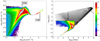 |
Fig. 1 Phase diagrams. Left panel: Phase diagram (pressure, P, vs. gas density, nH) of case A. The WNM and CNM regions are labeled. Right panel: Dependence of the ionization fraction, Xe, obtained with Eq. (6), vs the gas temperature, T. Here, the CR ionization rate is set to the value of ζH (see Sect. 2.4). Colors in both panels correspond to the log10 of the density of points as shown by the same color bar on the right. The gray part of the right-panel plot shows the voxels that were artificially set to Xe = 1 (see the two black arrows) as they strongly depart from the assumptions that justify the use of Eq. (6). See main text for details. |
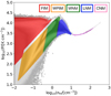 |
Fig. 2 Phase diagram as in the left panel of Fig. 1 for case A but with colors delimiting the regions corresponding to each gas phase as defined in Table 3. |
Volume fractions per gas phase depending on the model.
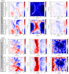 |
Fig. 3 Maps of rotation measure (RM) in units of rad m−2 obtained within the full length of the simulated cube for cases A and B with two amounts of ionization rates (ζ, see encapsulated panels on the left). The LOS changes along the x or y or z axes going from left to right, respectively. The dynamic range of the color bars is only positive when the integration axis is along the mean magnetic-field orientation (central panels in the first two rows from the top and right panels in the two bottom rows). |
3.2 Impact of B and ne on rotation measure
The physical interpretation of RM values, as those shown in the maps above, is complicated by the degeneracy between ne and the LOS-component of B (hereafter, B‖), as well as the path-length along the LOS (see Eq. (5)). While veritably a problematic issue with radio observations of diffuse polarized emission (e.g., Jelić et al. 2014; Lenc et al. 2016; Van Eck et al. 2017; Thomson et al. 2019; Turić et al. 2021), the degeneracy between ne and В‖ can be sometimes circumvented in the case of pulsar measurements (e.g., Smith 1968; Rand & Kulkarni 1989; Han et al. 1999; Han 2006; Sobey et al. 2019). In particular, pulsars give access to the dispersion measure (DM), defined in units of pc cm−3 as  , where d is the distance to the pulsar and r is the LOS. Combining DM with RM, in units of rad m−2, allows us to estimate the density-weighted average strength of В‖ in units of μG as follows:
 (7)
(7)
In this section, we investigate our simulations and consider whether we are able to discriminate magnetic fields from electrons in the synthetic observations of RMH. In Fig. 5, we show maps of the LOS-average of B‖ (hereafter, 〈B‖〉sim) computed along the y axis in case A, as well as the corresponding electron-column density (Ne).
Visually, the map of RMH (see central panel in the second row from the top of Fig. 3) is strongly correlated with the structure of 〈B‖〉sim and with that of Ne mostly toward the densest regions. The Pearson correlation coefficients (Rp) between RMH and 〈B‖〉sim, or Ne, are 0.95 and 0.84, respectively. The 2D histograms encoding these correlations are shown in Fig. 6, where the distributions of 〈B‖〉sim (in blue) and Ne (in red) are normalized to their 99th percentile.
In Fig. A.1, we present the same 2D histograms but for different integration axes and for case B. In all explored scenarios the values of RMH appear tightly correlated with those of 〈B‖〉sim. In the case of Ne, the correlation measured by Rp is generally weaker or absent (see left panels of Fig. A.1). It is not negligible when integration axis is along the main magnetic-field orientation.
Finally, we notice (as shown in Fig. 7) that from Eq. (7) we are able to give a reliable estimate of 〈B‖〉sim using 〈B‖〉pul, regardless of the integration axis. We produced this plot by accounting for 200 LOSs randomly chosen within the simulated boxes. The number of LOSs is not key to validate Eq. (7). The scatter of the 200 LOSs is comparable along all integration axes and shows that 〈B‖〉pul and 〈B‖〉sim are consistent within 1 σ (see inset in Fig. 7).
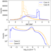 |
Fig. 4 Comparison between Case A and B. Top: histograms of the ratios of RM obtained with a high ionization rate (ζH = 2.6 × 10⁻¹⁶ s−1) and low ionization rate (ζL = 1.7 × 10⁻¹⁷ s−1) for cases A and B, in blue and orange, respectively. Histograms with different transparencies correspond to integration axes, x, y, and z, from thick to light curves, respectively. Bottom: histograms of the gas density for cases A and B. |
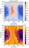 |
Fig. 5 Maps of the LOS-average magnetic field (top) and the electron column density (Ne, bottom) for case A integrated along the y axis. |
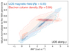 |
Fig. 6 2D histograms showing the correlation between RMH (see Fig. 3), and the maps of the LOS-average magnetic field (blue) and the electron column density (red). The ordinate axis shows the corresponding values normalized to their 99th percentile. From light to dark colors, contours correspond to number of pixels of 50, 100, 500, 1000, 2000. Person correlation coefficients (Rp) are written. As an example, we show case A integrated along the y axis. |
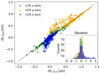 |
Fig. 7 Correlation between 〈B‖〉sim and 〈B‖〉pul for case A. A one-to-one dashed line is overlaid. The inset shows the deviation of 〈B‖〉pul from 〈B‖〉sim defined as (〈B‖〉sim − 〈B‖〉pul)/σsim, where σsim is the standard deviation of 〈B‖〉sim. |
3.3 Multiphase gas contribution to rotation measure
The range of RM depends on the phase distribution of the gas in the simulations (see Sect. 2.5). The five phases that we defined above are unevenly distributed in the cubes and show a distinct morphology depending on their mean gas density and temperature (see Table 3).
In Fig. 8, we show RGB images of NH maps corresponding to the cold (CNM+LNM), warm (WNM + WPIM), and hot (FIM) phases for two different integration axes of case A. All phases appear to be affected by the shell collision. While the hot and warm phases are mostly structured on a large scale (as expected), the coldest and densest phases show small-scale structures that are the consequence of thermal instability in the WNM.
The morphology of gas phases is highly correlated and complementary, although not necessarily co-spatial. The edges of each NH map appear aligned among phases. In order to quantify this, we applied histograms of oriented gradients (HOG6, Soler et al. 2019) to the NH maps obtained for each distinct phase. The basic principle of HOG is to provide a statistical estimate of the spatial correlation (morphological alignment) between two maps assuming that the local appearance and shape of a map can be fully characterized by the distribution of its local intensity gradients or edge directions. To evaluate the correlation we used the HOG output parameter defined as the projected Rayleigh statistics (V, see Eq. (C.1) in Bracco et al. 2020). The V parameter is a number that represents the likelihood that the gradients of two maps are mostly parallel. Larger values of V correspond to stronger alignment. As noticed by Soler et al. (2019), it is not possible to draw conclusions from the values of V alone, but its statistical significance can be assessed by comparing a given V value to others obtained in maps with similar statistical properties.
Because of the different volume filling fractions of the hot, warm, and cold phases (see Table 4), the surface area covered by the NH values of the former is significantly larger than the latter. Thus, when computing HOG, we normalized our V values to the amount of pixels where the NH of CNM is not zero. The normalized V values for case A are shown in Fig. 9. We studied the correlation among all phases for the three integration axes; V correctly shows no correlation with a Gaussian random field (labeled as “Random” in the figure). As shown in Fig. 9, the closer the phases are to each other in the phase space, the more alike their maps will appear.
This multiphase and multiscale structure in the simulations has an impact on the values of RMH, since not all phases contribute the same to the rotation measure. For each gas phase, we computed RM maps using only voxels belonging to that phase. In Fig. 10, for case A, we show the distributions of the relative contribution of each phase to the total RMH. We notice that the share of RMH among phases depends on the integration axis (see also Fig. A.2 for case B). Moreover, in case A the phases that contribute the most to the total RMH are WNM and WPIM, in spite of their lower Xe compared to FIM. The same is not true for case B, where FIM dominates the total RMH. In our simulations, CNM and LNM are generally found (as expected) to be negligible phases to the rotation measure.
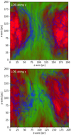 |
Fig. 8 RGB images showing the contribution to the column density structure of the cold phases (blue, CNM + LNM), the warm and partially ionized phases (green, WNM + WPIM), and the fully ionized phase (red, FIM) as defined in Table 3. Two different LOS for case A are shown. |
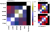 |
Fig. 9 Maps of the normalized projected Rayleigh statistics obtained with HOG (in colors) between the column density map of each phase as labeled in the figure. One random map for reference is also considered. Three different lines of sight of case A are shown. Larger values correspond to a higher degree of correlation. |
3.4 Mock observations of Faraday tomography
The imprint of each gas phase on the rotation measure also has an impact on the observed synchrotron polarized emission. As detailed in Sect. 2.2, we produced mock observations of synchrotron emission – total and polarized – both as a function of v and, through Faraday tomography, of ϕ. We chose a FWHM of the PSF of a few arcminutes (~7′) to be roughly comparable with that of LOFAR7, placing the simulated cubes at a hypothetical distance between 500 and 600 pc8. In the right panels of Fig. 11 we show, as an example, both Stokes I (top) and PI (bottom) at 150 MHz obtained for case A integrated along the y axis in units of mJy PSF−1. At 150 MHz we retrieve, at most, only 20% of Stokes I in polarization (PI150/I150 has a median value of 16%). The observed depolarization is due to the combined effects of the beam and of differential Faraday rotation in the cubes. The latter also introduces small-scale structure in polarization that is not observed in Stokes I.
This can be better more easily seen on the left of Fig. 11, where the 2D angular power spectra, p(k), of Stokes I and PI are shown. We notice that p(k) of Stokes I has a bump at about k ~ 0.03. This is likely due to the prominent filamentary structure in the middle that has a typical width of ~30 px. Both power spectra are affected by the beam at the largest k values. The power spectrum of Stokes I is steeper than that of PI with power-law indices in k space of −3.9 and −2.5, respectively. We checked that such difference found at 150 MHz is not observed at higher frequency (~20 GHz), where Faraday rotation is negligible.
The effect of differential Faraday rotation in polarization is more impressive when looking at Faraday tomographic data of PI as a function of ϕ. For case A, (integrated along the y axis) Fig. 12 illustrates three slices of PI in units of mJy PSF−1 RMSF−1 at given ϕ of 0, 1, and 2 rad m−2, respectively. The apparent resemblance of our mock observations of Faraday tomography with actual data of polarized diffuse emission detected with LOFAR is striking (e.g., Jelić et al. 2014; Van Eck et al. 2017; Turić et al. 2021). Regions of high PI emission show patchy and filamentary structures close to linear, narrow, and depolarized features that highly resemble the so-called depolarization canals found in real data (e.g., Haverkorn et al. 2003; Jelić et al. 2018). A detailed analysis of these features in our simulations will be the subject of future work. Here, we limit ourselves to exploring the statistics of the Faraday tomographic cubes using the Faraday moments first introduced by Dickey et al. (2019) to study Galactic polarized emission above 300 MHz with the Galactic Magneto-Ionic Medium Survey. Using Eqs. (5), (6), and (7) presented in Dickey et al. (2019) we define the moments M0, M1, and M2 that encode the total PI in the Faraday tomographic cube, the mean-weighted ϕ, and its corresponding variance, respectively. For the same simulations as those shown in Fig. 12, we present the moments in Fig. 13. M0 and  are strongly correlated to each other, while M1 shows distinct patterns. As also recently discussed by Erceg et al. (2022) in the analysis of the LoTSS survey, the values of
  trace complex lines of sight resulting from differential Faraday rotation.
The structure of M1 should be a proxy of the RM along the LOS. However, as can be seen by comparing the map of M1 with that of RMH (see Fig. 3) differences arise. These differences are caused by differential Faraday rotation. In Fig. 14 we compare M1 and RMH for the projections along the coordinate axes of case A. We show both 2D (top row) and 1D histograms of their relative ratio (RMH/M1, bottom row). The 2D histograms indicate a spread of M1 values around the M1 ∝ 0.5 RMH relation, regardless of the integration axis. However, the histograms of the ratio reveal that a value of the peak greater than unity (~2) is only observed when the integration axis is along the mean direction of the B field.
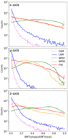 |
Fig. 10 Histograms of the relative contribution to the total rotation measure (RMH(total)) of each gas phase (RMH(phase)), as defined in Table 3 for case A. Colors are defined in the central panel. |
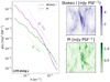 |
Fig. 11 Synthetic observations of synchrotron emission at 150 MHz: maps of Stokes I (top-right panel) and polarized intensity (PI, bottom-right panel), with corresponding angular power spectra (left panel). As an example, only case A integrated along the y axis is shown. |
3.5 Multiphase gas contribution to polarized intensity
As just shown, differential Faraday rotation strongly affects the amount of PI that can be detected at low radio frequencies. Since differential Faraday rotation depends on the multiphase structure of the intervening ISM, in this section we investigate what is the contribution of each gas phase (see Sect. 2.5) to PIϕ.
We addressed this question by studying the correlation between the morphological structure in the maps of PIϕ and each NH map introduced in Sect. 3.3. We used the V parameter from HOG to quantify the relative alignment between the local gradients of PIϕ with those of the total gas column density, NH, of each phase. As explained in detail in Appendix B, because of the shape of the RMSF, we weighted the V parameter from HOG with the ratio between the maximum value of PIϕ at a given slice and the maximum value of the full Faraday tomographic cube. As a null-test reference, we also studied the correlation between PIϕ with a map produced from a Gaussian random field, for which no morphological correlation is expected. We chose a Gaussian random field characterized by a power-law power spectrum with index of −2.7 so to introduce some multi-scale structure in the random map.
In Fig. 15, we show the resulting V parameter as a function of ϕ for all gas phases and integration axes of case A. Most of PI appears correlated with the structure of NH at low absolute values of ϕ. The correlation with the different gas phases significantly depends on the integration axis. Generally speaking, all phases show morphological correlation with PI compared to the random test, although the correlation is the strongest for WNM, WPIM, and FIM. Interestingly, the WNM and WPIM are those that correlate the most for the integration along the y axis. This is not true when the LOS is along the z axis (shell collision seen face on). In this case all phases appear poorly correlated with PI except for the FIM.
The synthetic PI that survives the differential Faraday rotation in our simulations shows a complex correlation among gas phases that strongly depends on the choice of the integration axis. In order to bridge our models with real observables, rather than with NH maps, we also studied the morphological correlation between PIϕ and synthetic observations of brightness temperature, Tb, of optically thin HI emission, as first presented in Bracco et al. (2020) with real data. We used the publicly available code BT-21cm9 that, given the simulated nH, T, and LOS velocity, produces estimates of Tb, as a function of local-standard-of-rest velocity (VLSR), in units of K following standard radiative transfer of HI (e.g., Spitzer 1978; Miville-Deschênes & Martin 2007).
We quantified the correlation between PIϕ and Tb(VLSR) using HOG. We built maps of the normalized V parameter, as explained above and in Appendix B, for all cases and integration axes. These maps are shown in Fig. 16 as a function of ϕ and VLSR.
The appearance of the V-parameter maps shows strong correlation between PIϕ and Tb(VLSR) for low absolute values of ϕ, as is expected based on Fig. 15 as well. The dependence on VLSR is not as well defined. This is due to the dominant contribution of WNM over LNM or CNM (see Table 4). The WNM has wide spectroscopic lines (Wolfire et al. 2003), which give rise to bright elongated features in the V-parameter maps. Figure 16 shows that, at least for the WNM phase, we are able to reproduce the observed correlation between PI and HI emission, as reported in Bracco et al. (2020).
We notice that this correlation highly depends on both integration axis and on the physical scenario taken into account. As expected, the correlation between PI and Tb is the strongest when the LOS integration occurs perpendicular both to the mean magnetic-field direction and to the shell-collision axis, as for case A with the LOS along the x axis. In case B, the correlation between PI and Tb is always lower than case A. This is due to the different physical evolution of the phases. In particular, as also listed in Table 4, the WNM phase in case B occupies almost half of the simulated volume compared to case A. In case B, the two shells collide along the mean magnetic field so that gas can transition more rapidly from the WNM to colder phases.
4 Discussion
Our study shows, for the first time, how important it is to account for the mutual interaction among ISM gas phases in order to model diffuse polarization detected at low radio frequencies. Nevertheless, we acknowledge the limitations of the analytical, steady-state, approach we used to define ne and to identify the five gas phases listed in Table 3. We have commented on the strong parametric dependence of ne on the value of ζ (see Sect. 2.4), which requires more detailed studies on CR propagation models across the multiphase ISM (e.g., Padovani et al. 2018; Kempski & Quataert 2022). Moreover, time-dependent chemistry should be considered in order to properly account for the ionization state of warm and cold gas phases (e.g., de Avillez et al. 2020), which inevitably affects the process of differential Faraday rotation (Rappaz et al. 2022). However, the error we made when applying Eq. (6) only underestimates the true amount of ionized gas (de Avillez & Breitschwerdt 2012). This means that in this work, we have provided lower limits to the Faraday rotation from the multiphase and ionized ISM that has an impact on the observed synchrotron polarization at low radio frequencies. Despite the caveats behind the estimate of ne, we stress that our approach is a step forward in modeling low-frequency synchrotron polarization affected by Faraday rotation based on MHD simulations. To our knowledge, this work is the first attempt to study synthetic observations at low frequency using simulations that include distinct gas phases ranging over several orders of magnitude in T and nH.
Previous works have accomplished the task of numerically studying the complexity of Faraday rotation and tomography. However, they have been limited to isothermal cases, expressing ne as a constant fraction of nH (e.g., Basu et al. 2019; Seta & Federrath 2021). This is possibly the reason why in Seta & Federrath (2021) these aforementioned authors could not generally apply Eq. (7) to derive 〈B‖〉sim from 〈B‖〉pul. As they considered an isothermal ideal MHD simulation, a much tighter correlation between B and ne could be seen, introducing a possible bias on the weighting of B along the LOS. In our models, on the contrary (as detailed in Sect. 3.2), B and ne are not correlated, validating Eq. (7).
Compared to the works mentioned above, we have produced more realistic models in terms of the properties of the multiphase gas, despite the very specific choice of our modeled physical scenario, namely that of two colliding super shells. Large-scale and shell-like polarization structures in the radio band have been extensively observed across tens of degrees in the sky, often referred to as loops (e.g., Berkhuijsen 1971; Vidal et al. 2015; Planck Collaboration XXV 2016; Thomson et al. 2021; Panopoulou et al. 2021). One of such structures, Loop III (e.g., Spoelstra 1972; Paseka 1993), represents the dominant structure in polarization within the largest mosaic of the LoTSS survey presently done and presented in Erceg et al. (2022). These loops are likely the result of multiple supernova explosions as those simulated by Ntormousi et al. (2017) and considered in this work. We believe that the choice of our case study is well motivated by observational evidence, although we recognize that our results and conclusions cannot be easily generalized to any MHD process in the ISM.
In Sect. 3.3, we addressed the key question about which gas phase might be the most relevant for the observed values of RMH. It is important to stress that the answer to this fundamental question is highly dependent on the physical scenario (cases A and B) and on the LOS integration axis. It is difficult to provide one simple rule of thumb based on our study, which means that in a general context, special care should be applied to interpreting RM observations. Broadly speaking, the warm, partially or fully ionized phases are those that dominate RM over the coldest and most neutral ones. However, we cannot exclude the possibility that this results from the very low volume filling fraction of CNM and LNM in the simulations (see Table 4). We also found a similar result when considering the gas-phase contribution to PI in Sect. 3.5. Interestingly, the contribution from WNM and WPIM is never negligible compared to that of FIM. This supports the idea, already proposed by Heiles & Haverkorn (2012), that Faraday rotation and low-frequency polarization, rather than recombination lines like Hα, could be a powerful probe of partially ionized gas, which presently challenges our understanding of structure formation in the local ISM (e.g., Jenkins 2013; Gry & Jenkins 2017). Moreover, the role of WNM is also highlighted by the correlation found between PI and Tb in Fig. 16. This result is reminiscent of the observational analysis of the LOFAR data done by Bracco et al. (2020), where PI was found morphologically correlated with Tb of HI data from the Effelsberg telescope (Winkel et al. 2016).
The choice of the LOS integration axis, however, has a huge impact on our results, particularly related to the anisotropy introduced by the mean-magnetic field direction in the simulations. We notice that several observables may provide an indication for this main source of anisotropy. First of all, the correlation between PI and Tb is the strongest when the LOS is perpendicular to the mean-magnetic field direction. This could be the case, as suggested by Zaroubi et al. (2015) and Jelić et al. (2018), for the observed correlation found between LOFAR polarization and tracers of neutral ISM in the surroundings of the 3C 196 field (Bracco et al. 2020; Turić et al. 2021). We must comment, however, on the lack of correlation between the simulated PI and the cold phases (CNM and LNM) in contrast to what was reported in Bracco et al. (2020), and previously in Van Eck et al. (2017) using data of interstellar dust extinction. The authors claimed that most of the correlation between the neutral medium (both probed by HI and dust) and LOFAR diffuse polarization was coming from CNM. This discrepancy between observations and simulations remains an open issue. Most likely, because of the very low fraction of CNM in these simulations, we are not able to quantitatively address the role of CNM. More work with simulations is needed to solve this inconsistency.
The anisotropy related to the mean magnetic field direction is also observable using the RMH/M1 ratio as a proxy. As shown in Fig. 14, we suggest that a peak of the distribution of RMH/M1 different than unity could be indicative of looking along the mean-magnetic field. However, this result is dependent upon our ability to define RMH and M1 for a common LOS volume in actual, low-frequency data. The slope of 2 in the correlation plot between RMH and M1 is in turn well understood in terms of differential Faraday rotation in Faraday thick structures (Burn 1966; Ordog et al. 2019; Erceg et al. 2022).
The effect of differential Faraday rotation is also revealed by the structures of Stokes I and PI at 150 MHz presented in Sect. 3.4. The 2D angular power spectra of the two maps are significantly different, with that of the PI map being flatter. The small-scale structure in polarization introduced by differential Faraday rotation is a characteristic feature only observable at these low radio frequencies. We notice that real LOFAR data show no (or nearly none) Stokes I counterpart to the diffuse polarized emission detected across all fields of view observed so far (Jelić et al. 2014, Jelić et al. 2015; Van Eck et al. 2017; Turić et al. 2021). As is known from previous Westerbork polarized observations (Wieringa et al. 1993), the missing short spacings in radio interferometers affect the large-scale emission of Stokes I more severely than that of PI, where the small-scale polarized structure survives.
A more careful analysis with simulations, including realistic models for the instrumental characteristics of LOFAR (e.g., by using OSKAR10 as in Mort et al. 2017), is beyond the scope of this work and will be part of future studies.
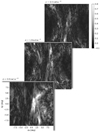 |
Fig. 12 Mock observations of Faraday tomography: maps of PI in units of mJy PSF−1 RMSF−1 as a function of Faraday depth, ϕ. The grey scale is the same in all three maps. As an example, case A is shown integrated along the y axis. |
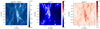 |
Fig. 13 Faraday moments (M0, M1, |

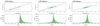 |
Fig. 14 Correlation diagrams between RMH and M1 (top row) together with the histograms of their ratio (bottom row). In the top panels, the M1 = RMH/2 line is shown in gray. In the bottom panels, the vertical blue and red lines correspond to ratios of 1 and 2, respectively. Three different lines of sight of case A are shown. |
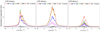 |
Fig. 15 Correlation analysis between PIϕ and the NH maps of each different gas phase (see the encapsulated legend) based on the projected Rayleigh statistics obtained with HOG. As a reference, the correlation with a random map is also shown in black. Three different LOS of case A are shown. |
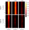 |
Fig. 16 Normalized V parameter from HOG between synthetic maps of the PI as a function of ϕ and of the HI brightness temperature, Tb, as a function of Vlsr. The corresponding LOS integration axis and physical scenario are labeled. The color scale is the same for all panels. |
5 Summary and conclusion
Faraday tomographic data below 200 MHz from the LOFAR telescope are challenging our understanding of the multiphase and magnetized ISM (e.g., Jelić et al. 2014; Zaroubi et al. 2015; Van Eck et al. 2017; Bracco et al. 2020). In this work, we present the first-ever analysis of synthetic data derived from MHD numerical simulations of Faraday tomography including multiphase ISM with temperatures and densities varying over more than four orders of magnitude.
We produced mock observations of differential Faraday rotation of synchrotron polarized emission between 115 MHz and 170 MHz, reaching values of Faraday depth similar to those observed with LOFAR in the Galactic ISM between −10 and +10 rad m−2. We used simulations of two colliding super shells produced by stellar feedback presented in Ntormousi et al. (2017).
The main results of our study are as follows. Realistic MHD simulations reveal that the coexistence of gas phases (from fully ionized to cold neutral media, CNM) is key to interpreting data affected by differential Faraday rotation observed at low radio frequency. The multiphase ISM leaves its imprint both in the analysis of rotation measure data and of Faraday tomographic data. In the case of rotation measure, our analysis shows that most of its structure is related to the structure of the intervening magnetic field. However, the contribution of the electron density is not negligible. In particular, we found that the warm and partially ionized phases (WNM and WPIM) may represent a large contribution to the observed rotation measure. Similarly, we found that these phases also contribute to most of the polarized intensity (PI) detected between 115 MHz and 170 MHz.
All results strongly depend on the LOS integration axis and on the physical scenario under study. We explored two different cases, in which the super-shell collision axis is either perpendicular or parallel (cases A and B, respectively) to the mean-magnetic field direction in the simulations. Using synthetic spectroscopic observations of atomic hydrogen (HI), we found that the correlation between WNM and PI is the strongest for case A, when the LOS is perpendicular to the mean-magnetic field direction and to the shell-collision axis. This result supports the interpretation already provided to explain the observational correlation found between LOFAR data and HI data toward the 3C 196 field (Kalberla & Kerp 2016; Bracco et al. 2020). On the other hand, regardless of the LOS, we found that our simulations always validate (within 1-σ deviation) the phenomenological derivation of the line-of-sight average magnetic-field strength as proposed in studies of Galactic pulsars (e.g., Sobey et al. 2019).
One open issue that arises from our work is that our simulations do not show a strong relation between PI and CNM structures, while the analysis of real observations hints at the possibility of one (Van Eck et al. 2017; Bracco et al. 2020). We notice that this inconsistency may be related to the low volume fraction of CNM in our simulations (a few %). However, we cannot exclude that other physical processes, not captured by the assumptions we made to model the ionization state of the ISM, or, otherwise, not related to the specific super-shell scenario, may be at play as a means of explaining the CNM issue.
As discussed in this pioneering exploratory study, additional work on MHD simulations is needed in order to investigate more carefully the complexity of the multiphase and magnetized ISM and its imprint on low-frequency polarization. Such an effort will be crucial for Galactic magnetism studies at low radio frequencies and interpreting data from future large-scale surveys both from LOFAR in the north (Shimwell et al. 2017, 2022) and from the Square Kilometre Array and its precursors in the south (Dewdney et al. 2009).
Acknowledgements
We are grateful to the anonymous referee for his/her comments. We are thankful to M.-A. Miville-Deschênes, P. Hennebelle, F. Boulanger, and J.D. Soler for useful discussions. A.B. acknowledges the support from the European Union’s Horizon 2020 research and innovation program under the Marie Skłodowska-Curie Grant agreement no. 843008 (MUSICA). A.B. is also deeply grateful to Delphine for maternal patience and profound inspiration: “Qué he sacado con el lirio, que plantamos en el patio, no era uno el que plantaba, eran dos enamorados, ay ay ay”. A.B. welcomes Elio to this turbulent world. V.J., L.T. and A.E. acknowledge support by the Croatian Science Foundation for the project IP-2018-01-2889 (LowFreqCRO). V.J. and L.T. also acknowledge support by the Croatian Science Foundation for the project DOK-2018-09-9169. E.N. is supported by the ERC Grant “Interstellar” (Grant agreement 740120). The authors acknowledge Interstellar Institute’s program “The Grand Cascade” and the Paris-Saclay University’s Institut Pascal for hosting discussions that nourished the development of the ideas behind this work. This research made use of Astropy (http://www.astropy.org), a community-developed core Python package for Astronomy (Astropy Collaboration 2013, 2018).
Appendix A Supplementary figures
In this appendix we present figures that support some of the results presented in Sect. 3.2 and Sect. 3.3.
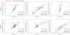 |
Fig. A.1 2D histograms showing the correlation between RMH and the maps of the LOS-average magnetic field (blue) and the electron column density (red) as in Fig. 6 but for lines of sight (LOS) along the x and z axes for case A (top row) and for all LOS axes for case B (bottom row). |
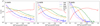 |
Fig. A.2 Histograms of the relative contribution to the total rotation measure of each gas phase as in Fig. 10, but for case B. Colors are defined in the central panel. |
Appendix B Rotation measure spread function and HOG
As mentioned in Sect. 3.5, the use of HOG with maps of PIϕ must take into account the shape of the RMSF resulting from low-frequency Faraday tomography.
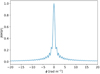 |
Fig. B.1 Rotation measure spread function used in this work to perform Faraday tomography. |
The RMSF of the synthetic Faraday spectra at LOFAR frequencies has side lobes (see Fig. B.1), which produce leakage from polarized intensity at a given ϕ over the full Faraday spectrum. This means that the structure of PIϕ reproduces itself at the peak of each side lobe in Faraday space. Thus, since in our analysis we did not introduce polarization noise, which, if large enough, can hide the side-lobe leakage, we faced the problem of identifying the right ϕ values for which PIϕ would truly correlate with any of the NH maps or Tb maps.
As an example, in Fig. B.2 we show how the same plot as the one presented in the middle panel of Fig. 9 would look like without weighting the V parameter from HOG to the ratio between the maximum value of PIϕ at a given slice in the Faraday cube and the maximum value of the full Faraday cube.
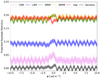 |
Fig. B.2 Correlation analysis between PIϕ and NH as in Fig. 15 but without normalizing the V parameter from HOG to the ratio between the maximum value of PIϕ at a given slice in the Faraday cube and the maximum value of the full Faraday tomographic cube. |
If on the one hand one could still identify the relative contribution of each phase to PIϕ, on the other hand it would not be possible to distinguish the right range of ϕ that would correspond to the morphological alignment between PIϕ and the NH maps of the different gas phases.
References
- Astropy Collaboration (Robitaille, T.P., et al.) 2013, A&A, 558, A33 [NASA ADS] [CrossRef] [EDP Sciences] [Google Scholar]
- Astropy Collaboration (Price-Whelan, A.M., et al.) 2018, AJ, 156, 123 [NASA ADS] [CrossRef] [Google Scholar]
- Basu, A., Fletcher, A., Mao, S.A., et al. 2019, Galaxies, 7, 89 [NASA ADS] [CrossRef] [Google Scholar]
- Beck, R. 2015, A&Ar, 24, 4 [Google Scholar]
- Beck, R., Chamandy, L., Elson, E., & Blackman, E.G. 2019, Galaxies, 8, 4 [NASA ADS] [CrossRef] [Google Scholar]
- Bellomi, E., Godard, B., Hennebelle, P., et al. 2020, A&A, 643, A36 [NASA ADS] [CrossRef] [EDP Sciences] [Google Scholar]
- Berkhuijsen, E.M. 1971, PhD thesis, Leiden Observatory, Leiden University, The Netherlands [Google Scholar]
- Bracco, A., Jelic, V., Marchal, A., et al. 2020, A&A, 644, A3 [Google Scholar]
- Brentjens, M.A., & de Bruyn, A.G. 2005, A&A, 441, 1217 [NASA ADS] [CrossRef] [EDP Sciences] [Google Scholar]
- Burn, B.J. 1966, MNRAS, 133, 67 [Google Scholar]
- Davies, R.D., Watson, R.A., & Gutierrez, C.M. 1996, MNRAS, 278, 925 [NASA ADS] [CrossRef] [Google Scholar]
- de Avillez, M.A., & Breitschwerdt, D. 2012, ApJ, 756, L3 [NASA ADS] [CrossRef] [Google Scholar]
- de Avillez, M.A., Anela, G.J., Asgekar, A., Breitschwerdt, D., & Schnitzeler, D.H.F.M. 2020, A&A, 644, A156 [NASA ADS] [CrossRef] [EDP Sciences] [Google Scholar]
- Dewdney, P.E., Hall, P.J., Schilizzi, R.T., & Lazio, T.J.L.W. 2009, IEEE Proc., 97, 1482 [NASA ADS] [CrossRef] [Google Scholar]
- Dickey, J.M., Landecker, T.L., Thomson, A.J.M., et al. 2019, ApJ, 871, 106 [NASA ADS] [CrossRef] [Google Scholar]
- Erceg, A., Jelic, V., Haverkorn, M., et al. 2022, A&A, 663, A7 [NASA ADS] [CrossRef] [EDP Sciences] [Google Scholar]
- Ferrière, K. 2020, Plasma Phys. Controlled Fusion, 62, 014014 [CrossRef] [Google Scholar]
- Field, G.B. 1965, ApJ, 142, 531 [NASA ADS] [CrossRef] [Google Scholar]
- Fitzpatrick, E.L., & Spitzer, L., J. 1997, ApJ, 475, 623 [NASA ADS] [CrossRef] [Google Scholar]
- Ginzburg, V.L., & Syrovatskii, S.I. 1964, The Origin of Cosmic Rays (London: Pergamon Press) [Google Scholar]
- Gry, C., & Jenkins, E.B. 2017, A&A, 598, A31 [NASA ADS] [CrossRef] [EDP Sciences] [Google Scholar]
- Guzmán, A.E., May, J., Alvarez, H., & Maeda, K. 2011, A&A, 525, A138 [NASA ADS] [CrossRef] [EDP Sciences] [Google Scholar]
- Han, J.L. 2006, Chinese J. Astron. Astrophys. Suppl., 6, 211 [NASA ADS] [CrossRef] [Google Scholar]
- Han, J.L., Manchester, R.N., & Qiao, G.J. 1999, MNRAS, 306, 371 [NASA ADS] [CrossRef] [Google Scholar]
- Haslam, C.G.T., Salter, C.J., Stoffel, H., & Wilson, W.E. 1982, A&AS, 47, 1 [Google Scholar]
- Haverkorn, M., Katgert, P., & de Bruyn, A.G. 2003, A&A, 403, 1031 [NASA ADS] [CrossRef] [EDP Sciences] [Google Scholar]
- Heiles, C., & Haverkorn, M. 2012, Space Sci. Rev., 166, 293 [NASA ADS] [CrossRef] [Google Scholar]
- Hennebelle, P., & Inutsuka, S.-I. 2019, Front. Astron. Space Sci., 6, 5 [NASA ADS] [CrossRef] [Google Scholar]
- Indriolo, N., Neufeld, D.A., Gerin, M., et al. 2012, ApJ, 758, 83 [NASA ADS] [CrossRef] [Google Scholar]
- Jelic, V., de Bruyn, A.G., Mevius, M., et al. 2014, A&A, 568, A101 [NASA ADS] [CrossRef] [EDP Sciences] [Google Scholar]
- Jelic, V., de Bruyn, A.G., Pandey, V.N., et al. 2015, A&A, 583, A137 [NASA ADS] [CrossRef] [EDP Sciences] [Google Scholar]
- Jelic, V., Prelogovic, D., Haverkorn, M., Remeijn, J., & Klindzic, D. 2018, A&A, 615, L3 [NASA ADS] [CrossRef] [EDP Sciences] [Google Scholar]
- Jenkins, E.B. 2013, ApJ, 764, 25 [NASA ADS] [CrossRef] [Google Scholar]
- Kalberla, P.M.W., & Kerp, J. 2016, A&A, 595, A37 [NASA ADS] [CrossRef] [EDP Sciences] [Google Scholar]
- Kempski, P., & Quataert, E. 2022, MNRAS, 514, 657 [NASA ADS] [CrossRef] [Google Scholar]
- Kim, C.-G., & Ostriker, E.C. 2017, ApJ, 846, 133 [NASA ADS] [CrossRef] [Google Scholar]
- Kim, C.-G., Kim, W.-T., & Ostriker, E.C. 2008, ApJ, 681, 1148 [NASA ADS] [CrossRef] [Google Scholar]
- Koyama, H., & Inutsuka, S.-I. 2002, ApJ, 564, L97 [Google Scholar]
- Krishnarao, D., Haffner, L.M., Benjamin, R.A., Hill, A.S., & Barger, K.A. 2017, ApJ, 838, 43 [NASA ADS] [CrossRef] [Google Scholar]
- Lenc, E., Gaensler, B.M., Sun, X.H., et al. 2016, ApJ, 830, 38 [NASA ADS] [CrossRef] [Google Scholar]
- Longair, M.S. 2011, High Energy Astrophysics (Cambridge: Cambridge University Press) [CrossRef] [Google Scholar]
- Marchal, A., Miville-Deschênes, M.-A., Orieux, F., et al. 2019, A&A, 626, A101 [NASA ADS] [CrossRef] [EDP Sciences] [Google Scholar]
- Miville-Deschênes, M.A., & Martin, P.G. 2007, A&A, 469, 189 [NASA ADS] [CrossRef] [EDP Sciences] [Google Scholar]
- Mort, B., Dulwich, F., Razavi-Ghods, N., de Lera Acedo, E., & Grainge, K. 2017, MNRAS, 465, 3680 [NASA ADS] [CrossRef] [Google Scholar]
- Mozdzen, T.J., Bowman, J.D., Monsalve, R.A., & Rogers, A.E.E. 2017, MNRAS, 464, 4995 [NASA ADS] [CrossRef] [Google Scholar]
- Mozdzen, T.J., Mahesh, N., Monsalve, R.A., Rogers, A.E.E., & Bowman, J.D. 2019, MNRAS, 483, 4411 [NASA ADS] [CrossRef] [Google Scholar]
- Neufeld, D.A., & Wolfire, M.G. 2017, ApJ, 845, 163 [NASA ADS] [CrossRef] [Google Scholar]
- Neufeld, D.A., Goicoechea, J.R., Sonnentrucker, P., et al. 2010, A&A, 521, L10 [CrossRef] [EDP Sciences] [Google Scholar]
- Ntormousi, E., Dawson, J.R., Hennebelle, P., & Fierlinger, K. 2017, A&A, 599, A94 [NASA ADS] [CrossRef] [EDP Sciences] [Google Scholar]
- Ordog, A., Booth, R., Van Eck, C., Brown, J.-A., & Landecker, T. 2019, Galaxies, 7, 43 [NASA ADS] [CrossRef] [Google Scholar]
- Orlando, E. 2018, MNRAS, 475, 2724 [NASA ADS] [CrossRef] [Google Scholar]
- Padovani, M., & Galli, D. 2018, A&A, 620, L4 [NASA ADS] [CrossRef] [EDP Sciences] [Google Scholar]
- Padovani, M., Galli, D., & Glassgold, A.E. 2009, A&A, 501, 619 [NASA ADS] [CrossRef] [EDP Sciences] [Google Scholar]
- Padovani, M., Galli, D., Ivlev, A.V., Caselli, P., & Ferrara, A. 2018, A&A, 619, A144 [NASA ADS] [CrossRef] [EDP Sciences] [Google Scholar]
- Padovani, M., Bracco, A., Jelic, V., Galli, D., & Bellomi, E. 2021, A&A, 651, A116 [NASA ADS] [CrossRef] [EDP Sciences] [Google Scholar]
- Panopoulou, G.V., Dickinson, C., Readhead, A.C.S., Pearson, T.J., & Peel, M.W. 2021, ApJ, 922, 210 [CrossRef] [Google Scholar]
- Paseka, A.M. 1993, AZh, 70, 258 [NASA ADS] [Google Scholar]
- Planck Collaboration XXV. 2016, A&A, 594, A25 [NASA ADS] [CrossRef] [EDP Sciences] [Google Scholar]
- Rand, R.J., & Kulkarni, S.R. 1989, ApJ, 343, 760 [NASA ADS] [CrossRef] [Google Scholar]
- Rappaz, Y., Schober, J., & Girichidis, P. 2022, MNRAS, 512, 1450 [NASA ADS] [CrossRef] [Google Scholar]
- Redfield, S., & Linsky, J.L. 2004, ApJ, 613, 1004 [NASA ADS] [CrossRef] [Google Scholar]
- Reich, P., & Reich, W. 1986, A&AS, 63, 205 [NASA ADS] [Google Scholar]
- Reissl, S., Brauer, R., Klessen, R.S., & Pellegrini, E.W. 2019, ApJ, 885, 15 [NASA ADS] [CrossRef] [Google Scholar]
- Rybicki, G.B., & Lightman, A.P. 1979, Radiative processes in astrophysics [Google Scholar]
- Saury, E., Miville-Deschênes, M.A., Hennebelle, P., Audit, E., & Schmidt, W. 2014, A&A, 567, A16 [NASA ADS] [CrossRef] [EDP Sciences] [Google Scholar]
- Seta, A., & Federrath, C. 2021, MNRAS, 502, 2220 [NASA ADS] [CrossRef] [Google Scholar]
- Shaw, G., Ferland, G.J., Srianand, R., et al. 2008, ApJ, 675, 405 [NASA ADS] [CrossRef] [Google Scholar]
- Shimwell, T.W., Röttgering, H.J.A., Best, P.N., et al. 2017, A&A, 598, A104 [NASA ADS] [CrossRef] [EDP Sciences] [Google Scholar]
- Shimwell, T.W., Hardcastle, M.J., Tasse, C., et al. 2022, A&A, 659, A1 [NASA ADS] [CrossRef] [EDP Sciences] [Google Scholar]
- Smith, F.G. 1968, Nature, 220, 891 [NASA ADS] [CrossRef] [Google Scholar]
- Snowden, S.L., Egger, R., Freyberg, M.J., et al. 1997, ApJ, 485, 125 [NASA ADS] [CrossRef] [Google Scholar]
- Sobey, C., Bilous, A.V., Grießmeier, J.M., et al. 2019, MNRAS, 484, 3646 [NASA ADS] [CrossRef] [Google Scholar]
- Sokoloff, D.D., Bykov, A.A., Shukurov, A., et al. 1998, MNRAS, 299, 189 [NASA ADS] [CrossRef] [Google Scholar]
- Soler, J.D., Beuther, H., Rugel, M., et al. 2019, A&A, 622, A166 [NASA ADS] [CrossRef] [EDP Sciences] [Google Scholar]
- Spitzer, L. 1978, Physical processes in the interstellar medium [Google Scholar]
- Spoelstra, T.A.T. 1972, A&A, 21, 61 [NASA ADS] [Google Scholar]
- Sun, X.H., Reich, W., Waelkens, A., & Enßlin, T.A. 2008, A&A, 477, 573 [NASA ADS] [CrossRef] [EDP Sciences] [Google Scholar]
- Thomson, A.J.M., Landecker, T.L., Dickey, J.M., et al. 2019, MNRAS, 487, 4751 [NASA ADS] [CrossRef] [Google Scholar]
- Thomson, A.J.M., Landecker, T.L., McClure-Griffiths, N.M., et al. 2021, MNRAS, 507, 3495 [NASA ADS] [CrossRef] [Google Scholar]
- Turic, L., Jelic, V., Jaspers, R., et al. 2021, A&A, 654, A5 [NASA ADS] [CrossRef] [EDP Sciences] [Google Scholar]
- Van Eck, C.L., Haverkorn, M., Alves, M.I.R., et al. 2017, A&A, 597, A98 [NASA ADS] [CrossRef] [EDP Sciences] [Google Scholar]
- van Haarlem, M.P., Wise, M.W., Gunst, A.W., et al. 2013, A&A, 556, A2 [NASA ADS] [CrossRef] [EDP Sciences] [Google Scholar]
- Vidal, M., Dickinson, C., Davies, R.D., & Leahy, J.P. 2015, MNRAS, 452, 656 [NASA ADS] [CrossRef] [Google Scholar]
- Voss, R., Diehl, R., Hartmann, D.H., et al. 2009, A&A, 504, 531 [NASA ADS] [CrossRef] [EDP Sciences] [Google Scholar]
- Waelkens, A., Jaffe, T., Reinecke, M., Kitaura, F.S., & Enßlin, T.A. 2009, A&A, 495, 697 [NASA ADS] [CrossRef] [EDP Sciences] [Google Scholar]
- Wang, J., Jaffe, T.R., Enßlin, T.A., et al. 2020, ApJS, 247, 18 [NASA ADS] [CrossRef] [Google Scholar]
- Wieringa, M.H., de Bruyn, A.G., Jansen, D., Brouw, W.N., & Katgert, P. 1993, A&A, 268, 215 [NASA ADS] [Google Scholar]
- Winkel, B., Kerp, J., Flöer, L., et al. 2016, A&A, 585, A41 [NASA ADS] [CrossRef] [EDP Sciences] [Google Scholar]
- Wolfire, M.G., Hollenbach, D., McKee, C.F., Tielens, A.G.G.M., & Bakes, E.L.O. 1995, ApJ, 443, 152 [NASA ADS] [CrossRef] [Google Scholar]
- Wolfire, M.G., McKee, C.F., Hollenbach, D., & Tielens, A.G.G.M. 2003, ApJ, 587, 278 [CrossRef] [Google Scholar]
- Zaroubi, S., Jelic, V., de Bruyn, A.G., et al. 2015, MNRAS, 454, L46 [NASA ADS] [CrossRef] [Google Scholar]
The term “intrinsic” refers to the synchrotron emission at low radio frequencies without the effect of Faraday rotation.
Here  are the normal vectors of the orthonormal base that defines the simulated data cubes.
I.e. number of electrons per unit energy, time, area, and solid angle.
The superscripts L and H refer to “low” and “high”, respectively.
LOFAR observations have a FWHM of 4′ (e.g., Jelić et al. 2014).
We notice that if this distance was lower, the non-orthonormal projection of the cube should be taken into account. In our case, at a distance of 575 pc, the angular size of the voxels changes at most between 2.4′ and 1.8′.
All Tables
Summary of the properties of the 5123 simulated cubes from Ntormousi et al. (2017).
Criteria in temperature (T) and ionization fraction (Xe) that define the different gas phases.
All Figures
|
Fig. 1 Phase diagrams. Left panel: Phase diagram (pressure, P, vs. gas density, nH) of case A. The WNM and CNM regions are labeled. Right panel: Dependence of the ionization fraction, Xe, obtained with Eq. (6), vs the gas temperature, T. Here, the CR ionization rate is set to the value of ζH (see Sect. 2.4). Colors in both panels correspond to the log10 of the density of points as shown by the same color bar on the right. The gray part of the right-panel plot shows the voxels that were artificially set to Xe = 1 (see the two black arrows) as they strongly depart from the assumptions that justify the use of Eq. (6). See main text for details. |
| In the text | |
|
Fig. 2 Phase diagram as in the left panel of Fig. 1 for case A but with colors delimiting the regions corresponding to each gas phase as defined in Table 3. |
| In the text | |
|
Fig. 3 Maps of rotation measure (RM) in units of rad m−2 obtained within the full length of the simulated cube for cases A and B with two amounts of ionization rates (ζ, see encapsulated panels on the left). The LOS changes along the x or y or z axes going from left to right, respectively. The dynamic range of the color bars is only positive when the integration axis is along the mean magnetic-field orientation (central panels in the first two rows from the top and right panels in the two bottom rows). |
| In the text | |
|
Fig. 4 Comparison between Case A and B. Top: histograms of the ratios of RM obtained with a high ionization rate (ζH = 2.6 × 10⁻¹⁶ s−1) and low ionization rate (ζL = 1.7 × 10⁻¹⁷ s−1) for cases A and B, in blue and orange, respectively. Histograms with different transparencies correspond to integration axes, x, y, and z, from thick to light curves, respectively. Bottom: histograms of the gas density for cases A and B. |
| In the text | |
|
Fig. 5 Maps of the LOS-average magnetic field (top) and the electron column density (Ne, bottom) for case A integrated along the y axis. |
| In the text | |
|
Fig. 6 2D histograms showing the correlation between RMH (see Fig. 3), and the maps of the LOS-average magnetic field (blue) and the electron column density (red). The ordinate axis shows the corresponding values normalized to their 99th percentile. From light to dark colors, contours correspond to number of pixels of 50, 100, 500, 1000, 2000. Person correlation coefficients (Rp) are written. As an example, we show case A integrated along the y axis. |
| In the text | |
|
Fig. 7 Correlation between 〈B‖〉sim and 〈B‖〉pul for case A. A one-to-one dashed line is overlaid. The inset shows the deviation of 〈B‖〉pul from 〈B‖〉sim defined as (〈B‖〉sim − 〈B‖〉pul)/σsim, where σsim is the standard deviation of 〈B‖〉sim. |
| In the text | |
|
Fig. 8 RGB images showing the contribution to the column density structure of the cold phases (blue, CNM + LNM), the warm and partially ionized phases (green, WNM + WPIM), and the fully ionized phase (red, FIM) as defined in Table 3. Two different LOS for case A are shown. |
| In the text | |
|
Fig. 9 Maps of the normalized projected Rayleigh statistics obtained with HOG (in colors) between the column density map of each phase as labeled in the figure. One random map for reference is also considered. Three different lines of sight of case A are shown. Larger values correspond to a higher degree of correlation. |
| In the text | |
|
Fig. 10 Histograms of the relative contribution to the total rotation measure (RMH(total)) of each gas phase (RMH(phase)), as defined in Table 3 for case A. Colors are defined in the central panel. |
| In the text | |
|
Fig. 11 Synthetic observations of synchrotron emission at 150 MHz: maps of Stokes I (top-right panel) and polarized intensity (PI, bottom-right panel), with corresponding angular power spectra (left panel). As an example, only case A integrated along the y axis is shown. |
| In the text | |
|
Fig. 12 Mock observations of Faraday tomography: maps of PI in units of mJy PSF−1 RMSF−1 as a function of Faraday depth, ϕ. The grey scale is the same in all three maps. As an example, case A is shown integrated along the y axis. |
| In the text | |
|
Fig. 13 Faraday moments (M0, M1, |
| In the text | |
|
Fig. 14 Correlation diagrams between RMH and M1 (top row) together with the histograms of their ratio (bottom row). In the top panels, the M1 = RMH/2 line is shown in gray. In the bottom panels, the vertical blue and red lines correspond to ratios of 1 and 2, respectively. Three different lines of sight of case A are shown. |
| In the text | |
|
Fig. 15 Correlation analysis between PIϕ and the NH maps of each different gas phase (see the encapsulated legend) based on the projected Rayleigh statistics obtained with HOG. As a reference, the correlation with a random map is also shown in black. Three different LOS of case A are shown. |
| In the text | |
|
Fig. 16 Normalized V parameter from HOG between synthetic maps of the PI as a function of ϕ and of the HI brightness temperature, Tb, as a function of Vlsr. The corresponding LOS integration axis and physical scenario are labeled. The color scale is the same for all panels. |
| In the text | |
|
Fig. A.1 2D histograms showing the correlation between RMH and the maps of the LOS-average magnetic field (blue) and the electron column density (red) as in Fig. 6 but for lines of sight (LOS) along the x and z axes for case A (top row) and for all LOS axes for case B (bottom row). |
| In the text | |
|
Fig. A.2 Histograms of the relative contribution to the total rotation measure of each gas phase as in Fig. 10, but for case B. Colors are defined in the central panel. |
| In the text | |
|
Fig. B.1 Rotation measure spread function used in this work to perform Faraday tomography. |
| In the text | |
|
Fig. B.2 Correlation analysis between PIϕ and NH as in Fig. 15 but without normalizing the V parameter from HOG to the ratio between the maximum value of PIϕ at a given slice in the Faraday cube and the maximum value of the full Faraday tomographic cube. |
| In the text | |
Current usage metrics show cumulative count of Article Views (full-text article views including HTML views, PDF and ePub downloads, according to the available data) and Abstracts Views on Vision4Press platform.
Data correspond to usage on the plateform after 2015. The current usage metrics is available 48-96 hours after online publication and is updated daily on week days.
Initial download of the metrics may take a while.