| Issue |
A&A
Volume 662, June 2022
|
|
|---|---|---|
| Article Number | A66 | |
| Number of page(s) | 30 | |
| Section | Catalogs and data | |
| DOI | https://doi.org/10.1051/0004-6361/202141570 | |
| Published online | 17 June 2022 | |
Stellar labels for hot stars from low-resolution spectra
I. The HotPayne method and results for 330 000 stars from LAMOST DR6★
1
Max-Planck-Institut für Astronomy,
Königstuhl 17,
69117
Heidelberg,
Germany
e-mail: This email address is being protected from spambots. You need JavaScript enabled to view it.
2
Institute for Advanced Study,
Princeton,
NJ
08540,
USA
3
Department of Astrophysical Sciences, Princeton University,
Princeton,
NJ
08544,
USA
4
Observatories of the Carnegie Institution of Washington,
813 Santa Barbara Street,
Pasadena,
CA
91101,
USA
5
Research School of Astronomy & Astrophysics, Australian National University,
Canberra
ACT 2611,
Australia
6
LMU München, Universitätatssternwarte,
Scheinerstr. 1,
81679
München,
Germany
7
Institute for Astronomy, University of Hawaii at Manoa,
2680 Woodlawn Drive,
Honolulu,
HI
96822,
USA
8
Center for Astrophysics, Harvard & Smithsonian,
Cambridge,
MA
02138,
USA
9
National Astronomical Observatories, Chinese Academy of Sciences,
Beijing
100012,
PR China
10
University of Chinese Academy of Sciences,
Beijing
100049,
PR China
11
Institut für Astro- und Teilchenphysik, Universität Innsbruck,
Technikerstrasse 25,
6020
Innsbruck,
Austria
12
Institute of Astronomy,
KU Leuven, Celestijnenlaan 200D,
3001
Leuven,
Belgium
13
South-Western Institute for Astronomy Research, Yunnan University,
Kunming
650500,
PR China
Received:
16
June
2021
Accepted:
19
February
2022
Abstract
We set out to determine stellar labels from low-resolution survey spectra of hot stars, specifically OBA stars with Teff ≳ 7500 K. This fills a gap in the scientific analysis of large spectroscopic stellar surveys such as LAMOST, which offers spectra for millions of stars at R ~ 1800 and covers 3800 Å ≤ λ ≤ 9000 Å. We first explore the theoretical information content of such spectra to determine stellar labels via the Cramér-Rao bound. We show that in the limit of perfect model spectra and observed spectra with signal-to-noise ratio ~50–100, precise estimates are possible for a wide range of stellar labels: not only the effective temperature, Teff, surface gravity, log g, and projected rotation velocity, vsin i, but also the micro-turbulence velocity,vmic, helium abundance, NHe/Ntot, and the elemental abundances [C/H], [N/H], [O/H], [Si/H], [S/H], and [Fe/H]. Our analysis illustrates that the temperature regime of Teff ~ 9500 K is challenging as the dominant Balmer and Paschen line strengths vary little with Teff. We implement the simultaneous fitting of these 11 stellar labels to LAMOST hot-star spectra using the Payne approach, drawing on Kurucz’s ATLAS12/SYNTHE local thermodynamic equilibrium spectra as the underlying models. We then obtain stellar parameter estimates for a sample of about 330 000 hot stars with LAMOST spectra, an increase by about two orders of magnitude in sample size. Among them, about 260 000 have good Gaia parallaxes (ω/σω > 5), and their luminosities imply that ≳95% of them are luminous stars, mostly on the main sequence; the rest are evolved lower luminosity stars, such as hot subdwarfs and white dwarfs. We show that the fidelity of the results, particularly for the abundance estimates, is limited by the systematics of the underlying models as they do not account for nonlocal thermodynamic equilibrium effects. Finally, we show the detailed distribution of vsin i of stars with 8000–15 000 K, illustrating that it extends to a sharp cutoff at the critical rotation velocity, vcrit, across a wide range of temperatures.
Key words: techniques: spectroscopic / surveys / catalogs / stars: massive / stars: fundamental parameters / stars: abundances
The catalog is only available at the CDS via anonymous ftp to cdsarc.u-strasbg.fr (130.79.128.5) or via http://cdsarc.u-strasbg.fr/viz-bin/cat/J/A+A/662/A66
Hubble fellow.
© M. Xiang et al. 2022
 Open Access article, published by EDP Sciences, under the terms of the Creative Commons Attribution License (https://creativecommons.org/licenses/by/4.0), which permits unrestricted use, distribution, and reproduction in any medium, provided the original work is properly cited.
Open Access funding provided by Max Planck Society.
1 Introduction
Hot stars, here meaning stars with OBA spectral types or Teff ≳ 7500 K, are interesting objects for a number of reasons: they are tracers of young stellar populations in our Galaxy; they are intriguing laboratories for testing stellar structure and evolution scenarios; and they can be progenitors of and companions to black holes and supernovae. Recently, these stars have garnered more attention thanks to large sky low-resolution (R ~ 2000) spectroscopic surveys, such as the LAMOST Galactic surveys (Deng et al. 2012; Zhao et al. 2012) and the SDSS-V Milky Way Mapper (Kollmeier et al. 2017; Zari et al. 2021). LAMOST has collected R ~ 1800 optical spectra for thousands of stars identified as OB stars (Liu et al. 2019) and hundreds of thousands of A-type stars. The SDSS-V will yield spectra for many more OB stars in the next few years (Zari et al. 2021). Due to their high effective temperature, the spectra of hot stars show much weaker spectral features than those of cool stars. As a result, the latter have been the analytical focus of most Galactic archaeology surveys to date. Stellar parameter pipelines for large spectroscopic surveys have been mainly focused on FGK stars (e.g., Lee et al. 2008; Luo et al. 2015; Xiang et al. 2015, 2019; García Pérez et al. 2016; Casey et al. 2017; Ahumada et al. 2020; Buder et al. 2021; Steinmetz et al. 2020). Beside the easier measurements, the detailed abundances [X/H] of cool stars have been of particular interest as they are closer to the birth-material composition of the stars and can enable ‘‘chemical tagging’’. Furthermore, it has been shown that even low-resolution spectra can yield useful stellar labels, such as Teff, log g, and abundance [X/H] for >15 elements (Ting et al. 2017a,b; Xiang et al. 2019).
For hot stars, the surface abundances can be affected by stellar internal mixing processes, making them deviate significantly from the solar abundance scale (e.g., Przybilla et al. 2010; Ekström et al. 2012; Maeder et al. 2014; Martins et al. 2015; Pedersen et al. 2018; Aerts 2021) and rendering them less useful for inferences in Galactic archaeology. On the other hand, these mixing processes can make hot stars powerful probes of stellar evolution physics. Particularly, it has long been known that ‘chemically peculiar’ stars are common among hot stars (e.g., Renson & Manfroid 2009; Gray et al. 2016; Qin et al. 2019; Chojnowski et al. 2020; Xiang et al. 2020; Paunzen et al. 2021) and provide good constraints on stellar element transport processes (e.g., Talon et al. 2006; Vick et al. 2010; Michaud et al. 2015). Despite their interesting prospects, the parameters and detailed abundances of hot stars were only derived for relatively small samples, usually no larger than ~O(103) stars (e.g., Przybilla et al. 2008; Nieva & Przybilla 2012, 2014; Simón-Díaz & Herrero 2014; Kudritzki et al. 2016; Berger et al. 2018; Holgado et al. 2018).
The lack of a systematic analysis of hot-star spectra calls for flexible and sophisticated spectral modeling to deliver astro-physical labels for hot stars from the vast sets of low-resolution spectra collected by large sky surveys. This is particularly important for the LAMOST Galactic Survey as it has collected low-resolution spectra (R ~ 1800) for hundreds of thousands of OB A stars. Yet, a comprehensive and quantitative determination of stellar parameters and abundances for all these hot stars with LAMOST spectra does not exist, and we aim to provide it here.
In this work we demonstrate that R ~ 1800 spectra contain a wealth of astrophysical information for hot stars. We apply PAYNE (Ting et al. 2019) for an ‘industrial scale’ determination of stellar labels from a massive set of LAMOST hot-star spectra. Payne is a spectral model fitting tool with the ability to simultaneously determine many labels from the full spectra at modest computational expense. This is owed to the flexible neural-net-based spectral interpolation algorithm that can precisely interpolate spectra in high dimensions (Ting et al. 2019). Fitting the entire spectrum allows for an optimal use of its information content, and fitting all pertinent labels simultaneously ensures that label covariances, due to line blending, are correctly accounted for. We fit a large number (11) of labels to LAMOST spectra of probable hot stars – effective temperature (Teff), surface gravity (log g), microturbulence velocity (vmic), projected rotation velocity (vsin i), helium abundance (NHe/Ntot), and elemental abundances [C/H], [N/H], [O/H], [Si/H], [S/H], and [Fe/H]. We dub our modeling HOTPAYNE as the original PAYNE approach has been mostly applied to FGK stars; hot-star spectra are sufficiently different, so this spectral regime requires nontrivial modifications and testing, as we will show.
We adopt the Kurucz local thermodynamic equilibrium (LTE) spectra (Kurucz 1970, 1993, 2005) as our underlying model spectra to train the HOTPAYNE neural network spectral model. As nonlocal thermodynamic equilibrium (NLTE) effects and stellar winds play important roles for hot-star spectroscopy (e.g., Auer&Mihalas 1972; 1976, 1979, 1998; Hubeny & Lanz 1995; Kudritzki & Puls 2000; Lanz & Hubeny 2007; Przybilla et al. 2008, 2010; Hainich et al. 2019), our resultant label estimates, based on the Kurucz LTE model spectra, are therefore inevitably affected by non-negligible systematic errors. We address such systematics by comparing our results with literature values from high-resolution NLTE spectroscopic analyses for a sample of reference stars. We emphasize from the outset that the approach presented here deserves to be followed up with label determinations based on NLTE model spectra to obtain accurate label estimates, in particular of elemental abundances for these hot stars, which we will perform in a future study. Nonetheless, the internal precision of our LTE-based abundance estimates appears to be promising for a number of interesting applications, as presented in this study.
The paper is organized as follows. In Sect. 2 we introduce the LAMOST spectra for the sample of candidate hot stars. In Sect. 3 we explore the information content of such low-resolution spectra of hot stars. In Sect. 4 we derive stellar labels from the R ~ 1800 LAMOST spectra for >330000 hot stars. We present and discuss these results in Sect. 5, which is followed by a summary in Sect. 6.
2 LAMOST spectra of candidate hot stars
We compiled a sample of candidate hot stars with low-resolution (R ~ 1800) optical (λ ~ 3800-9000) spectra from the sixth data release (DR6)1 of the LAMOST Galactic surveys (Deng et al. 2012; Zhao et al. 2012; Liu et al. 2014); we refer to this initial list as candidates, as our subsequent spectral analysis reveals that some of them have low temperatures of Teff < 7000 K. The LAMOST Galactic surveys target millions of stars in the full color-magnitude diagram down to about 17.8 mag in the SDSS r band (Carlin et al. 2012; Liu et al. 2014; Yuan et al. 2015). As a key component of the LAMOST Galactic surveys, the LAMOST Spectroscopic Survey at the Galactic Anti-Center (LSS-GAC) uniformly samples stars in the (g−r, r) and (r − i, r) space. This uniform selection implies that stars in the low density regimes of the color-magnitude diagram (e.g., OB stars) are targeted with higher completeness (Liu et al. 2014; Yuan et al. 2015; Xiang et al. 2017; Chen et al. 2018), which results in a large sample of hot-star spectra with well-characterized completeness, located mostly in the Galactic anticenter direction. The LAMOST DR6 released 9 911 337 spectra, and each has a spectral classification with the LAMOST 1D pipeline (e.g., Luo et al. 2015). Among the 9 911 337 spectra, 9 231057 are classified as stars.
As summarized in Table 1, we define the hot-star candidates by the following three criteria. First, we adopted LAMOST DR6 stars that are classified as O, B, and A types according to the LAMOST pipeline. This is a total of 575 736 spectra.
Second, we cross-matched the LAMOST DR6 with a full-sky hot-star catalog (candidate OBA stars), devised using the same approach as in Zari et al. (2021), which is based on parallax, magnitudes, and colors from Gaia DR2 (Gaia Collaboration 2018) and the Two Micron All Sky Survey (2MASS; Skrutskie et al. 2006). The key difference is that Zari et al. (2021) based their OBA star catalog on Gaia Early Data Release 3 (eDR3; Gaia Collaboration 2021) and selected hot stars with a 2MASS Ks-band absolute magnitudes MK < 0mag. For our study, we adopted Gaia DR2 (consistent with LAMOST DR6) and have selected hot stars with MK < 3 mag. The cross-match led to 866 780 spectra in common.
Third, we adopted the LAMOST DR5 OB star catalog by Liu et al. (2019). It contains 26453 spectra also found in the LAMOST DR6 database.
About 35% of the spectra for the candidate stars selected with the Zari et al. (2021) method are classified as OBA types by the LAMOST pipeline. This number is reasonable as we set a loose cut in absolute magnitude by using MK < 3 mag. Utilizing a stricter cut of MK < 0 mag, Zari et al. (2021) suggested that about 45% of their hot-star candidates with LAMOST spectra have effective temperature higher than 9700 K, corresponding to a stellar type earlier than A0V. Equivalently, about 52% of the OBA-type spectra classified by the LAMOST pipeline are selected as hot-star candidates with the Zari et al. (2021) method. We note that the criteria of Zari et al. (2021) are mainly set to select hot stars earlier than B7V type, for which they have achieved a high completeness rate (8282/9083 when testing on the LAMOST OB stars). As here we apply the method to the O-, B-, and A-type stars, it is not surprising that we find a smaller completeness rate.
A simple union of these three source lists led to 1 163 410 spectra for hot-star candidates. These are for 844790 unique stars, as we keep the repeated observations in the database. Figure 1 shows the distribution of these stars in Galactic coordinates, along with the LAMOST survey footprint. Unsurprisingly, these hot-star candidates are concentrated toward the Galactic plane, which is expected since most hot stars are young stars. Many of the stars at high Galactic latitudes turn out to be hot old stars, such as hot subdwarfs (sdBs, sdOs) and blue horizontal branch (BHB) stars. The majority of the stars are toward the Galactic anticenter, as targeted by the LSS-GAC. There are also a moderate number of stars in the first and second Galactic quadrants toward the inner Galaxy, particularly in the Kepler field. Figure 2 shows the distribution of the Gaia G-band magnitude and the LAMOST spectral signal-to-noise ratio (S/N) for our sample of candidate stars. The G-band magnitudes cover a dynamic range of nearly 15 mag, and most of them are between ~10 and 18 mag, with a peak at around 14 mag. The S/N peaks at about 63 (log(S /N) ~ 1.8), but the median value is about 37 due to a significant low-S/N tail.
We corrected for the line-of-sight velocity derived from the LAMOST pipeline (Luo et al. 2015). All model fitting in this study will act on the normalized spectra. Specifically, all spectra were normalized by a smoothed version of themselves, derived by convolving the spectra with a Gaussian kernel of 50 Å width:
 (1)
(1)
 (2)
(2)
A similar spectral normalization approach was previously adopted in the analysis of the LAMOST low-resolution spectra (Ho et al. 2017; Xiang et al. 2019). It should be noted that this is different to the “continuum” normalization applied in high-resolution spectroscopic analysis. Rather than determining the real continuum, which is hard for the case of low-resolution spectra, the purpose of our spectral normalization is to ensure that the observation spectra and the model spectra are normalized in the same manner for spectral fitting. As the spectra are normalized to the mean flux smoothed in a broad window, the method is robust for spectra of low S/N. However, a mismatch between the model spectra and observation spectra could be raised from either sys-tematics of the former (Sect. 4) or interstellar absorption lines that presented solely in the latter. Such a mismatch will cause line profiles that differ between the normalized model and the observed spectra, causing systematic mismatch in the spectral fitting. To minimize this effect, we masked the hydrogen lines along with some other strong lines and the bands of interstellar absorption, by setting the weight of those pixels to be zero. By doing so, the resulting line profiles are consistent between models and observations, except for the cores of strong lines that suffer large model systematics.
Sources of the LAMOST DR6 hot-star candidates.
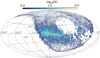 |
Fig. 1 On-sky distribution of our LAMOST DR6 hot-star candidates in Galactic coordinates (l, b). The map is centered on the Galactic anticenter (l = 180°, b = 0°). The thick line delineates the celestial equator (Dec = 0°), and lines of constant declination, Dec = ±30° and Dec = ±60°, are also shown. Colors indicate the logarithmic number of stars in each (l, b) cell of 0.2° × 0.2°. The distribution reflects both the LAMOST survey area and the candidate stars’ concentration to the Galactic plane, which is expected for young stars. |
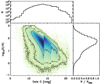 |
Fig. 2 Distribution of our LAMOST DR6 hot-star candidates in the Gaia G-band magnitude and LAMOST spectral S/N plane. The G-band magnitudes cover a dynamic range of nearly 15 magnitudes, and most of them are between G ~ 10 and 18 mag. The spectral S/N peaks at around 63 (log(S /N) ~ 1.8) but has a median value of 37 due to a significant low-S/N tail. The isodensity contours encompass 68.3, 95, and 99.7% of the sample stars, respectively, and the colors delineate the relative stellar number density, with darker colors representing higher density. |
3 The stellar label information content of low-resolution hot-star spectra
Understanding what parameters and abundances we should adopt for our spectral grid requires us to evaluate the information content of these spectra: that is, for which labels the spectra vary appreciably when labels vary and how covariate they are. One way to answer these questions is via calculating the Cramér-Rao (CR) bound (Cramér 1945; Rao 1945). The same approach was demonstrated by Ting et al. (2016, 2017a) and Sandford et al. (2020), who applied the CR bound to predict the (theoretical) precision of stellar label determination of FGK stars for different spectral resolutions and wavelength coverage.
The theoretical precision limit for a label estimate from a given spectrum depends on two aspects: (a) the gradient function of the spectra ∇l : = ∂fλ/∂l, which describes the response of the spectral flux fλ with respect to the change of stellar label l, and (b) the flux uncertainties and covariances of the spectra. Following Ting et al. (2017a), the CR bound thus can be described as
 (3)
(3)
where  is the inverse of the covariance matrix of the stellar labels, C−1 the inverse of the covariance of the normalized spectral flux, ∇if(λ1) the gradient spectra with respect to label i at λ1, and ∇if (λ2) the gradient spectra with respect to label j at λ2. The gradient spectra are calculated through finite model differencing.
As an example, Fig. 3 shows the gradient spectra ∂fλ/∂l computed for a fiducial B star with Teff = 18 000 K, log g = 4.0, and [Fe/H] = 0. The figure illustrates that hot stars are information rich. Besides the stellar parameters, there are numerous pixels in the LAMOST wavelength range (3800–9000 Å) that are informative for a few selected elements. Unsurprisingly, the most informative pixels for Teff and log g are the hydrogen lines, both Balmer and Paschen series, with moderate contributions from helium lines and metal lines, whereas the information for vsin i resides mostly at the cores of strong absorption lines. We also note that the spectral features do not necessarily need to come from the atomic transition of a species. For some elements, such as helium, the change of abundance can modify the overall atmosphere structure appreciably. This will in turn indirectly modify the strength of spectral features.
Although the figure demonstrates that many pixels contain valuable information for various labels, nonetheless the absolute changes for individual pixels are small in most cases: |∂fλ/∂l| changes rarely more than 1% even for abundance changes of a full dex. These subtle and mostly covariate changes of spectral features are what inspire us to adopt a technique for full spectral fitting, such as PAYNE, in the first place (see Sect. 4.2).
A realistic calculation of CR bound requires not only gradient spectra but also the assumed uncertainties of the spectral fluxes. For simplicity, for this theoretical exercise, we assume that the spectral measurements are independent among the adjacent pixels. We adopted a S/N variation with wavelength that is typical of B stars in LAMOST and scale that value to S /N = 100 at 4650 Å. Some assumptions of the CR bound calculation are undoubtedly optimistic. For example, the values and uncertainties among adjacent pixels in an observed spectrum can be correlated. Furthermore, the calculation assumes a perfect knowledge of the spectral models. Experience has shown that CR bound calculations can usually be attained within a factor of two despite these imperfections (e.g., Ting et al. 2019; Sandford et al. 2020). We emphasize that this exercise here aims only to determine what labels we should adopt for the spectral grid.
The CR bound, expressed by the diagonal terms of the CR matrix  is shown in Fig. 4 for our fiducial B star spectrum. The calculation predicts that, in the limit of spectral perfect knowledge, we should obtain measurements with precision of ~300 K for Teff, 0.03 dex for log g, 1% for NHe/Ntot, 1 km s−1 for vmic, and 8 kms−1 for vsin i from a typical LAMOST spectrum for a hot star. The CR bounds for element abundance are within 0.1 dex for a few elements with strong features, such as C, O, Si, and Fe. For other elements, such as N, Mg, and Al, the CR bounds are within 0.2 dex. Although the figure only presents the CR bounds for some selected elements (with atomic number no larger than Zn), all elements with atomic number smaller than Eu, except for Li, Be, B, F, V, and Co, are included for the CR bound computation. We omit all CR bounds that are larger than 10 dex. The CR bounds for Li, Be, B, F, V, and Co are discarded because their null gradients could cause numerical artifacts in the results. Finally, we note that here we adopt a B star as reference point for this study; the CR bound will obviously vary among different stellar types.
Figure 5 presents the covariances among the selected labels, reflecting in the off-diagonal term of the CR matrix Kij. As expected, the Teff and log g are strongly correlated, as their gradient spectra share many common spectral features (H and He lines). Similarly, the NHe/Ntot abundance estimate is strongly anticorrelated with Teff and log g. The [Si/H] and [S/H] are strongly correlated with vmic. The [C/H] and [N/H] are moderately correlated with Teff. The vsin i, [O/H] and [Fe/H] are not strongly correlated with any of the other labels. The nontrivial correlation between labels due to somewhat degenerate spectral features further demonstrates that the pertinent labels can be only be obtained by fitting all labels simultaneously through full spectral fitting.
To sum up, inspired by this exploration of the CR bounds for low-resolution spectra of hot stars, we chose to build a spectral model for these LAMOST spectra that depends on 11 labels, namely Teff, log g, vmic, vsin i, NHe/Ntot, [C/H], [N/H], [O/H], [Si/H], [S/H], and [Fe/H] (Sect. 4), as they are among labels we can derive from the spectra with the best precision.
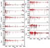 |
Fig. 3 Information content of low-resolution spectra for a B star. Each panel shows the gradient spectrum ∇l : = ∂fλ/∂l with respect to different labels, l, derived from finite differencing of Kurucz model spectra (black) at Teff = 18 000 K, log g = 4.0, [Fe/H] = 0, and vsin i = 100 km s−1. The gradient spectra generated from HOTPAYNE are overplotted in red, illustrating the robustness of HOTPAYNE: the good agreement to the Kurucz model suggests that HOTPAYNE determines the labels from the relevant features instead of harnessing the astrophysical correlations. For Teff, vmic, vsin i, and NHe/Ntot, the gradient spectra are multiplied by 1000 K in Teff, 5 km s−1 in vmic, 20 km s−1 in vsin i, and 0.05 in NHe/Ntot for better visibility. This figure shows that the diagnostic signatures of label changes are widely distributed across the optical spectral range. Nonetheless, most spectral features are subtle due to LAMOST’s spectral resolution and the high effective temperature of the star: most abundance signatures are at the 1% level, even for abundance changes of 1 dex. Useful information about hot stars can only be extracted from a global fit to the spectrum and a careful spectral modeling. |
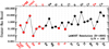 |
Fig. 4 Theoretical precision limits for stellar label determination from LAMOST of hot stars, expressed through the CR bound, |

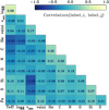 |
Fig. 5 Correlation coefficients among the stellar label estimates, predicted by the CR bound calculation (see Eq. (3)). These correlations were derived for the spectrum of a fiducial B-type star with Teff = 18 000 K, log g = 4.0, [Fe/H] = 0, and vsin i = 100 kms−1. Prominent among the correlations are those between estimates of Teff and log g, and between NHe/Ntot and both Teff and log g. The nontrivial correlations suggest that most spectral features are somewhat blended and thus call for a simultaneous fit of all pertinent labels to the entire spectrum. |
4 Stellar label determination
In this section we introduce our method of determining stellar labels for hot stars from the LAMOST spectra. This includes an introduction of the Kurucz model spectral library, the application of HOTPAYNE for the spectral fitting, as well as examinations of the resultant label estimates.
4.1 The Kurucz synthetic spectral library
We built a library of synthetic spectra generated with SYN-THE, using the Kurucz LTE atmospheric model calculated with ATLAS12 (Kurucz 1970, 1993, 2005). We considered 11 physical labels – Teff, log g, [Fe/H], vmic, vsin i, NHe/Ntot, and [X/H] for X = C, N, O, Si, and S for the spectral modeling. The parameter ranges are presented in Table 2. For Teff, log g, and [Fe/H], we sampled the grids from the MESA Isochornes and Stellar Tracks (MIST; Dotter 2016; Choi et al. 2016) uniformly in equivalent evolutionary phase. While the other labels were uniformly drawn within the given range for each label. For all other abundances not presented in Table 2 but are required to generate the synthetic spectra models, we simply scaled them with [Fe/H], assuming the solar abundance scale of Asplund et al. (2009). The model spectra were broadened according to the vsini value. To ensure the convergence of the model computation, we required that, at Rosseland mean opacities of τross = 0.1 and of τross = 1, the flux errors be smaller than 2% and the flux derivative errors be smaller than 20%. Also, we required the maximum variation in temperature for the inner atmospheric layers (40–80) between two iterations to be fractionally smaller than 10−4.
In total, we generated 10 127 Kurucz model spectra. The native model spectra generated with the SYNTHE have a resolving power of R = 500000, and we degraded them to match the line spread function (LSF) of the LAMOST spectra. We adopted a Gaussian profile for the LSF, the width of which is a wavelength-dependent function, approximated by a two-order polynomial for the blue and red spectrograph arms, separately. The LAMOST spectra have R ~ 1800 at 5000 Å (FWHM ~ 2.8 Å), but the detailed spectral LSF is found to vary from fiber to fiber and exposure to exposure (e.g., Xiang et al. 2015). To generate a range of realistic LSFs for the model grid, we assign a specific LSF for each model spectrum, using individual LAMOST LSFs derived from different exposures and fibers. The spectra are further broadened to their corresponding vsin i assuming rotational profiles with a constant limb darkening coefficient of 0.6 (Gray 1992; Hubeny & Lanz 2011).
Our LTE Kurucz models come with two caveats. First, for very hot (≳40 000 K) stars with either relatively high metallicity ([Fe/H] ≳ −0.25 dex) or relatively low log g values (≲4.0), those with very high CNO abundance values can lead to a low hydrogen fraction (e.g., <0.6). In this case, the model computations are hardly converged, which leads to a poor coverage in those parts of the parameter space.
Second, the model spectra are generated using the Kurucz 1D LTE atmospheric model. As mentioned in Sect. 1, it is known that the NLTE effect and stellar winds are non-negligible for hot stars, and especially strong for giants (e.g., Kurucz 1970; 1979, 1998; Hubeny & Lanz 1995; Lanz & Hubeny 2007; Hainich et al. 2019). In this work, we chose to apply the LTE model as a proof of concept. While the Kurucz model spectra may be less accurate than NLTE spectra, they are flexible in obtaining self-consistently computed model spectra across the broad parameter range we want, and they use relatively complete line lists. Nonetheless, as we demonstrate in the rest of the paper, further efforts based on NLTE model spectra are necessary in order to generate accurate elemental abundances.
4.2 HOTPAYNE
Payne is a full spectral fitting tool for stellar label determination built on several key ingredients: First, it trains a flexible spectral interpolation model based on a neural network that allows one to interpolate spectra precisely in high dimensions (e.g., ~20), Furthermore, Payne emphasizes the importance to generate models self-consistently. The self-consistency here refers to the fact that we always solve for the atmospheric structure before running the radiative transport for changes in any of the stellar labels. Secondly, Payne fits all labels of consideration simultaneously from the full spectra with the goal to make full use of the information in the spectra and to properly characterize the covariances of labels arose due to line blending effects. Such an effect is particularly prominent for low-resolution spectroscopy (Ting et al. 2019).
To train Payne, we divided the Kurucz spectral library into two sets, the “training set”, with 9115 spectra, and the validation test set, with 1012 spectra. We trained the neural-network model for the pixel-by-pixel spectral interpolation, predicting the flux at each wavelength as a continuous function of the labels. Our neural network model has two layers, each with 100 neurons, and the Sigmoid activation function is adopted to scale the input spectra. The training is carried out in the Pytorch environment, using the adaptive moment estimation algorithm (Kingma & Ba 2014). In the training process, we have 17 free parameters, including the 11 target stellar labels shown in Table 2, and six more coefficients describing the LSF (three for each of the blue and red arm, respectively) as introduced above. We also explored the possibility of deriving the macroturbulent velocity, vmacro, which reflects the contribution of the non-rotational line profile broadening (e.g., Simón-Díaz & Herrero 2014), on top of vsin i, but we found that the two parameters are too degenerate at the LAMOST resolution. We chose to only fit for vsin i in this work. Consequently, our vsin i estimates are likely contributed by both the rotational broadening and macroturbulence. Our estimates might overestimate the true vsin i in the case where the non-rotational broadening is comparable or stronger than the rotational broadening. For example, Simón-Díaz & Herrero (2014) found that for stars with vsin i < 120 kms−1, ignoring vmacro may lead to an overestimate of vsin i by ~25 km s-1 in general.
Figure 6 illustrates the precision of the spectral interpolation by HOTPAYNE, deduced from the test spectra. For all individual pixels of the 1012 test spectra, the overall dispersion of the residuals between the HOTPAYNE fits and the Kurucz model flux is 0.165%, which is equivalent to a spectral S/N of 600. For those pixels with normalized flux values smaller than 0.95, mostly the cores of strong H and He lines, the dispersion of the residuals is 0.586% (or equivalently, a S/N of 200). In other words, the interpolation errors from PAYNE are largely negligible given the typical S/N of LAMOST is lower than 200.
To assess the internal precision of stellar label determination with HOTPAYNE, we make a sanity check using the Kurucz test spectral sample. That is, we derived the stellar labels of the Kurucz test spectra using HOTPAYNE and then compared them to the true labels. We added noise to the test spectra (with S/N~ 100 at 4650 Å), as for the CR bound calculations. For reason that we elaborate on in Sect. 4.3, we adopted a fixed LSF by taking the mean LAMOST LSF and did not fit for them; we analyzed the LAMOST data the same way.
Figure 7 plots the differences (residuals) between the HOTPAYNE stellar label estimates and the true values as a function of the true Teff, and color-coded by the true values of the labels. On average, the model-to-model fits show that we can recover the stellar labels, except for the very metal poor end. A Gaussian fit to the residuals suggests that, on the whole, the internal precision is about 2.1% for Teff, 0.07 dex for log g, 1.2km s−1 for vmic, 12.1 km s−1 for vsin i, 0.02 for NHe/Ntot, 0.09 dex for [O/H], about 0.15 dex for [C/H], 0.18 dex for [Fe/H], 0.20dex for [Si/H], 0.26 dex for [N/H], and 0.39 dex for [S/H]. We note that for some labels such as [N/H] and [S/H], the error is partially dominated by a few outliers, a consequence of the strong variations in label precision across the parameter (Teff and [X/H]) space. For stars with Teff ~ 18 000 K and [Fe/H] ~ 0 dex, we find that the precision is consistent with the CR bound (Fig. 4) within a factor of two.
The precision of HOTPAYNE’s label estimates vary significantly with both Teff and [X/H]. For stars with Teff < 11000K, the log g residuals exhibit a strong negative trend with Teff, causing a Teff-dependent systematic bias in log g of up to about 0.2 dex at the low-Teff limit. A similar trend is also presented in the [Fe/H], [Si/H], and [S/H] panels, causing a Teff-dependent systematics of about 0.1 dex in [Fe/H], and larger values in [Si/H] and [S/H]. This trend reflects an imperfection of our spectral emulation for this cool part of the parameter space, probably due to either insufficiently flexible neural networks or nonopti-mal training process (e.g., gets stuck in a local minimum). There are also many more metal lines in the low-temperature spectra, which increase significantly the complexity of the emulation. At this cool end, our test shows that the NHe/Ntot estimates can be challenging but the NHe/Ntot estimates are robust for stars with Teff > 11000 K, because the He lines are more prominent at this temperature range. On the high-temperature side of Teff > 25 000 K, the Teff estimates exhibit a somewhat artificial trend, with an amplitude of <3%. However, we note that for such a high-temperature case, the NLTE effects may lead to much larger systematics in the Teff estimates (see Sect. 4.7). For the metal-poor stars of [X/H] ≲ −1 dex, the abundance estimates may suffer large deviations from the true values, especially for [C/H], [N/H], [O/H], and [S/H]. This is just the manifestation that, for metal-poor stars, the spectral features become too weak to allow for any abundance estimation. However, we note that in the real case of LAMOST survey, we do not expect that there are many hot stars with such a low metal-licity, except for some chemically peculiar stars with very low CNO abundances due to atomic diffusion (e.g., Michaud et al. 2015).
While the model-to-model fit remains optimistic, we caution that when fit to the LAMOST spectra, the fit is likely to incur larger uncertainties due to the mismatch between model and observed spectra due to model imperfections.
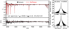 |
Fig. 6 Precision of the spectrum prediction by HOTPAYNE, which entails a neural-net-enabled interpolation among Kurucz model spectra. The left panels show the comparison between the Kurucz spectrum and its prediction by HOTPAYNE for a test star with Teff = 18 236 K, log g = 4.23, and [Fe/H] = 0.0. Top-right panel: distribution of flux residuals for all of our 1012 test spectra, each with 3801 pixels in the wavelength range of λλ3750–9000 Å. A Gaussian fit to the distribution yields a standard deviation of 0.165%. Bottom-right panel: analogous to the top-right panel, but only for pixels whose normalized spectral fluxes are smaller than 0.95, i.e., for strong absorption lines, mostly the cores of H and He lines. The standard deviation from a Gaussian fit is 0.586% for the strong absorption features. |
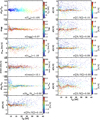 |
Fig. 7 Precision of the HOTPAYNE label estimates as a function of Teff. Plotted are the differences (residuals) between the labels from HOTPAYNE and the true values for a test set of Kurucz model spectra with S/N ~ 100, color-coded by the true values. The numbers marked in the figure are the dispersion derived from a Gaussian fit to the residuals. The precision of the HOTPAYNE label determination varies with Teff and [X/H]. For metal-poor stars of [X/H] < −1 dex, the [X/H] estimates may suffer large uncertainties. However, we note that in the real case of the LAMOST survey, we do not expect there to be many hot stars with such low metallicities. |
4.3 The line spread function
The LSF of the individual LAMOST spectra vary between fibers and between exposures, which is expected to have an impact on the stellar label determination (e.g., Xiang et al. 2015). By design, our HotPayne module can fit the LSF from the spectra simultaneously with the stellar labels. However, we found it challenging to determine the LSF from fitting Kurucz models to the LAMOST spectra, because such fits are impacted by even small, systematic line core mismatches owed to systemat-ics of the Kurucz models. A more sensible way is to take the LSF of each LAMOST spectrum derived from arc lamps and sky emission lines as input, and fix it in the HotPayne fitting. However, currently such LSF data for LAMOST spectra are still missing.
As a compromise, we instead adopted the mean LSF of the LAMOST spectra derived by the author using arc lamps and sky emission lines from the LSS-GAC DR2 (Xiang et al. 2017). We tested the impact of the fiber-to-fiber and exposure-to-exposure variations in the LSF on the stellar label determination by assigning each Kurucz test spectrum (Sect. 4.2) a unique LSF from the LSS-GAC DR2, and we fit them with the HotPayne model spectra with the mean LSF. We find that ignoring the variations in LSF will cause larger uncertainties on the vsin i estimates, which typically amount to 17 km s−1 (compared to the 12km s−1 from the mean LSF as shown in Fig. 7), as a consequence of the LSF and vsini covariance. For a minor number of spectra with very different LSF, the vsini estimates may differ by larger than 30 kms−1 from the results of the mean LSF. Whereas for the other labels, the LSF has only marginally effects on the HotPayne determination in most cases.
4.4 Initial estimates of Teff from line indices
To facilitate the spectral fitting with HotPayne to the LAMOST data set, we first made an initial estimate of Teff based on the indices (equivalent widths) of the Ca ii 3933 Å, H i and Caii 3967Å, and Hi 4101Å lines. To compute the line indices, we adopted the λ3912–3922 Å and λ3946–3956 Å windows for continuum estimates of the Ca ii 3933 line. Similarly, the continuum for H i+Ca ii 3967 Å is derived from the λ3946–3956 Å and λ3980–3990 Å windows, and the continuum for Hi 4101Å line is derived from the λ4080–4090 Å and λ4114–4124 Å windows.
We used a subset of 57 039 LAMOST spectra as the reference set to build an empirical relation between line indices and Teff. This reference set includes 16002 stars from the LAMOST OB sample of Liu et al. (2019), and the remaining ones are selected from the LAMOST and Zari et al. (2021) common star sample, the majority of which are A- and F-type stars according to the LAMOST classification. The Teff of these reference spectra are estimated with HotPayne assuming an initial Teff set to be the mean Teff of our training library spectra. For late F-type stars, the Teff estimates with HotPayne might be inaccurate as they are outside the Teff coverage of the Kurucz training set (i.e., cooler than <7500 K). We therefore adopted the Teff provided in Xiang et al. (2019) if it has smaller ;χ2 than the HotPayne fits. We fitted a three-order polynomial to this reference set, thereby predicting Teff from line indices. This yields the following relation:

where C3933, C3967, and C4101 are the equivalent widths of the Ca II 3933Å, H I+Ca II 3967Å, and Hi 4101Å lines, respectively. For OB stars, the Ca line index may suffer from some uncertainties due to interstellar absorption, but since our estimates from the line indices only serve as an initial guess to optimize the running time, such uncertainties have minimal impact on our final estimates.
4.5 Spectral masking and the spurious absence of early A-type stars
When fitting the LAMOST spectra, we also masked the wavelength windows with known telluric or interstellar medium absorption. In particular, we masked the known strong diffuse interstellar bands from the Diffuse Interstellar Band (DIB) directory (Hobbs et al. 2008), the Na I λ5890, 5896 doublet, and the Ca II K λ3933 line. We also discarded the blue (λ < 3820 Å) and red (λ > 8880 Å) edges of the LAMOST spectra, as well as the dichroic region (5700–6050 Å) of the blue and red arms of the LAMOST spectrographs. The masked wavelength regions are shaded in Fig. 8.
Our preliminary fits lead to resultant stellar parameters that exhibit a desert of early A-type and late B-type dwarf stars (9000 ≲ Teff ≲ 11000 K) in the Teff–log g diagram (left panel of Fig. 9). This desert is unexpected in the context of Galactic evolution and star formation/evolution scenarios. A careful inspection of the spectral models reveals that this artifact is possibly related to the change of signs in the gradient spectra of hydrogen lines for the A0-type stars. For A0 stars (Teff ~ 9500 K), the strength of hydrogen lines reaches a maximum, so that the gradient spectra of hydrogen lines for A0 stars reach a minimum, with absolute values close to 0 (see Fig. A.1). This causes an inflection point in the spectral gradient features of the hydrogen lines as a function of Teff. As a consequence, the parameter estimates are sensitive to the initial Teff values. Depending on the initial guesses from the line indices, the fits tend to pile up due to the “gradient gap”, causing the desert in the Teff-log g diagram as seen in the left panel of Fig. 9. These effects are illustrated in the right panel of Fig. 9.
As a remedy, we masked all hydrogen lines for label determination for these early A-type and late B-type stars. The masked regions are shown in the bottom panels of Fig. 8. Masking the hydrogen lines can reduce the spectral information content and lead to lower precision for the label determinations, particularly for Teff and log g. Nonetheless, an examination of the CR bound for early A-type stars suggests that the hydrogen-masked spectra are still able to yield robust estimates for many of the labels (see Fig. B.1). The Teff–log g diagram deduced for a subset of LAMOST stars after masking the hydrogen lines is shown in the middle panel of Fig. 9. Masking the hydrogen lines resolved the non-sensible desert. In order to benefit from the full spectral fitting as we can while mitigating the impact of hydrogen lines on the A0 stars, we combined the two sets of label estimates to give the ultimate label estimates2. The combination is carried out using the weighted mean value,
 (4)
(4)
where l1 and l2 represent the labels derived from spectra with and without the hydrogen lines masked, respectively. We adopted the Hann function as the weights for labels derived from the H-masked spectra,
 (5)
(5)
where x = Teff – 9500 K, and the Teff is that from the H-masked spectra. The weights for the labels derived from the full spectra are
 (6)
(6)
As for the smoothing length, for stars with  , we adopted a smoothing length L of 5000 K, such that ω1 = 0 for stars with
  . And for stars with
  , we adopted a length L of 3000 K, such that ω1 = 0 for stars with
  .
.
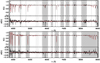 |
Fig. 8 Example of the HotPayne fit for a B-type star (top) and an early A-type star (bottom). The LAMOST spectra are shown in black, and the best-fit HotPayne models are shown in red. The masked telluric bands, the DIB, the interstellar absorption of Na and Ca, and the dichroic region are marked by shaded regions. For the case of early A-type stars, the wavelength windows of hydrogen lines (Balmer and Paschen series) are also masked (see text). |
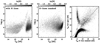 |
Fig. 9 Teff-log g diagrams for Teff derived from the LAMOST spectra without (left) and with (middle) the hydrogen lines masked. Right panel: direct comparison of the Teff estimates in the left and middle panels. The inclusion of hydrogen lines for the label determination causes an artificial desert of early A-type (and late B-type) dwarf stars in the Teff-log g diagram due to the reverse of spectral gradients |

4.6 Examination with repeat observations
About 30% of the LAMOST spectra are repeat observations of common targets (e.g., Yuan et al. 2015; Xiang et al. 2017). The label estimates from these repeated observations can differ due to a number of reasons, such as the photon noise, the fiber-to-fiber and temporal variation in the LSF, and imperfect calibration processes (e.g. flat-fielding, sky and scatter light subtraction, etc.). Comparing the label estimates among repeated observations thus gives an estimate of the precision of the label estimates3. To estimate the quality of our fit, we adopted only the repeated observations that have comparable (<20% difference) spectral S/N. The precision of the label is estimated through the square root of the dispersion among repeated observations.
The precision of our estimates as a function of S/N is shown in Fig. 10. The figure shows that, at S/N below 100, the photon noise dominates the spectral uncertainties, with the precision improve as 1/(S/N), as expected from the CR bound calculation. The precision only gradually improves beyond S /N > 100 because the instrument and calibration errors dominate the spectral uncertainties. In the case of S/N < 50, the label estimates have a precision of 700 K in Teff, 0.19 dex in log g, 4.1 km s−1 in vmic, 51.5km s−1 in vsin i, 0.03 in NHe/Ntot, 0.27 dex in [O/H], ~0.5 dex in [Si/H], and [Fe/H], > 1.0 dex in [C/H], [N/H], and [S/H]. Whereas in the case of S /N > 100, the uncertainties reduce to 260 K in Teff, 0.08 dex in log g, 0.85 km s−1 in vmic, 13.0km s−1 in vsin i, 0.01 in NHe/Ntot, ~0.20dex in [C/H], [N/H], and [S/H], ≲0.10dex in [O/H], [Si/H], and [Fe/H]. In general, these values for the case of S /N ≃ 100 are consistent with the CR bounds.
Sources of high-resolution optical spectra from ESO archives.
4.7 Comparison with literature
The LAMOST surveys mostly target stars fainter than 10 mag in the SDSS r-band; however, most of the literature stars are brighter. As a consequence, there is a lack of a meaningful sample of reference hot stars that have well-established parameters and abundances from high-resolution, NLTE-based spec-troscopy. For the current purpose, we compiled our reference stars from two sources, the first is a collection of high-resolution, NLTE-based stellar labels of 11 A-type and B-type stars from Przybilla et al. (2006, Przybilla et al. 2010), and Nieva & Przybilla (2012). These stars were not observed by the LAMOST survey but have available high-resolution full-optical spectra from the European Southern Observatory (ESO) science archive. We degraded them to the LAMOST resolution with the mean LSF to perform the label determination with HOTPAYNE. For verifying stellar parameters (Teff, log g, vsin i) of supergiants, our reference set contains four B-type supergiants, namely HD 41117, HD 52089, HD 52382, and HD 79186, whose reference parameters are from Haucke et al. (2018). Table 3 presents a summary of the sources of high-resolution spectra for these reference stars. Their stellar parameters and abundances from high-resolution NLTE analysis in literature are presented in Tables 4 and 5, respectively.
The other stars in our reference sample are slowly pulsating B-type (SPB) stars from Gebruers et al. (2021). The Gebruers et al. (2021) sample consists 20 SPB stars in the Kepler field, and with light curves from the Kepler mission (Borucki et al. 2010). The stellar labels of these SPB stars are estimated from high-resolution spectra, utilizing LTE-based stellar model spectra (Gebruers et al. 2021). Of the 20 SPB stars of Gebruers et al. (2021), 18 have LAMOST spectra from the LAMOST-Kepler project (De Cat et al. 2015; Fu et al. 2020). Due to their intrinsic brightness, these LAMOST spectra all have S /N > 200.
Figure 11 presents an one-to-one comparison of the labels estimates from HotPayne with their reference values for Teff, log g, and vsin i. The comparison suggests that our estimates for these labels are in decent agreement with the literature values, except for the Teff of stars hotter than 25 000 K. For these hot stars, our Teff estimates are systematically lower than the literature values by about 3000 K, due to the NLTE effects. The NLTE models generally predict stronger lines than LTE models (see Figs. C.1 and C.2). As a result, the LTE analysis favors a lower Teff for these hot stars. The log g shows good agreement with our results, demonstrating the ability of HOTPAYNE to distinguish giants from dwarfs. The A-type supergiant giant star HD 92207 exhibits large deviation in log g, as Przybilla et al. (2006) gives an estimate of 1.2 dex for log g while our estimate is 2.0 dex. This discrepancy is likely caused by NLTE effects, which are particularly strong for supergiants (e.g., Kudritzki 1976, 1979). The vsin i shows decent agreement with literature, particularly for stars rotating faster than 100 km s−1, demonstrating the ability of HOTPAYNE to distinguish fast rotating stars from slow rotating stars.
Figure 12 illustrates a similar comparison but vmic, NHe/Ntot, and [X/H]. The differences between the HOTPAYNE estimates and the literature values are plotted as a function of Teff of the stars. For stars hotter than 15 000 K, our estimates of vmic are systematically larger than the literature values by up to 10 km s−1, due to NLTE effect, which is more prominent for the hotter stars (see the appendix). At cooler end (Teff < 15000 K), our vmic estimates for dwarfs are in decent agreement with literature values. For example, for Vega (HD 172167), the literature vmic is 2kms−1, and we obtain 4.4 km s−1. Whereas for the A-type supergiants, our estimates are higher than literature values, again because of NLTE effect, which is more prominent for supergiants than for dwarfs. Although not shown here, for the LAMOST stars with Teff < 9000 K, our results exhibit a typical vmic of ~2kms−1, which is in line with expectations (e.g., Gebran et al. 2014). The NHe/Ntot is systematically overestimated by ~0.10, except for the A-type supergiants. This is due to NLTE effects, as explained above, NLTE models have deeper He lines than LTE spectra, which in turn favor lower NHe/Ntot estimates.
As for the abundances, the comparison reveals a Teff-dependent systematic trend in our abundance estimates, largely a consequence of NLTE effects. In particular, for stars with Teff > 25 000 K, our estimates are generally lower than the reference values by 0.3 dex for [Fe/H], 0.5–1.0dex for [C/H], [Si/H], and [S/H]. It should be noted that for HD 36512 (33 400K, in black, and barely visible in the plot), our estimates of [Si/H] and [Fe/H] are are erroneously low (<−2 dex). The exact cause is hard to be determined, but it is likely due to the imperfect fringing subtraction of spectra taken by the Ultraviolet and Visual Echelle Spectrograph (UVES). The effect is the most prominent for HD 36152. For stars of 11000 < Teff < 25 000 K, our [Fe/H] estimates are in decent agreement with Gebruers et al. (2021), but systematically higher than Przybilla et al. (2010); Nieva & Przybilla (2012). Both ours and Gebruers et al. (2021) are based on LTE models, and the good agreement validates our method, further elucidating that the differences with the other studies are largely due to the NLTE effect. We have only one star with NLTE abundances at Teff ~ 15000 K. Beside NLTE effects, imperfections of line lists may have also played a role for the difference. Particularly, for C we adopted the older line list of Jorgensen et al. (1996), which may need to be updated with more recent line lists (e.g., Masseron et al. 2014). The [O/H] seems to be in decent agreement with literature, except for the A-type super giants and the stars with Teff > 30000 K, both of which may have suffered strong NLTE effects. The reasonable agreement of [O/H] with literature values is not surprising, because oxygen has the most prominent features in the spectra (see Figs. C.1 and C.2). Nonetheless, it seems that even for [O/H], there can be a systematic uncertainty at a level of 0.2 dex from NLTE effects.
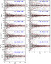 |
Fig. 10 Label differences between repeat observations as a function of S/N for stars with Teff > 10 000 K. Only repeat observations carried out on different observation nights and with S/N differences of less than 20 percent are adopted. The x axis shows the mean S/N of the repeat observations. The solid lines in red show the median differences as well as the standard deviations at different S/N. The numbers marked in the figure are precision (the scatter divided by |

Stellar parameters of our reference stars from literature.
Elemental abundances of our reference stars from NLTE analyses of high-resolution spectra.
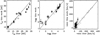 |
Fig. 11 Comparison of labels between the HOTPAYNE estimates and high-resolution spectroscopic results for our reference stars. For all the dots in black, the spectra are collected from the ESO archive (Table3) and degraded to the LAMOST resolution for stellar label determination with HotPayne. For these stars, the literature labels are adopted from Przybilla et al. (2006, 2010), Nieva & Przybilla (2012), and Haucke et al. (2018). Open squares represent the SPB stars of Gebruers et al. (2021), which have LAMOST observational counterparts. The Gebruers et al. (2021) high-resolution spectroscopic labels of these SPB stars are derived using LTE-based model spectra. The HOTPAYNE estimates show good agreements with the literature values. For stars with Teff > 25 000 K, the LTE-based estimation with HOTPAYNE underestimates the Teff due to NLTE effects. Similarly, the log g for supergiants (log g < 2) are overestimated due to the differences between the LTE and NLTE modeling. |
5 Results and discussion
5.1 The final sample
We applied HOTPAYNE to our 1 160000 LAMOST hot-star-candidate spectra. A considerable fraction of these candidates are found to be cool stars with Teff < 7000 K, due to contamination from our target selection. Since our Kurucz spectral model grid covers only Teff > 7500 K (Table 2), the labels for stars with Teff < 7500 K are estimated with HOTPAYNE via extrapolation. We therefore discarded all stars with Teff < 7000 K in our sample. We note that we chose to keep the stars with 7000 < Teff ≲ 7500 K because this regime was poorly investigated in previous efforts to estimate labels for FGK stellar sample (e.g., Xiang et al. 2019), and our labels might be useful for the general purpose.
We discarded results from spectra with S /N < 5 from our final catalog to ensure the precision of the label estimates. Furthermore, we found that the Teff estimates for a considerable number of (~5%) intrinsically cool (Teff < 7000 K) stars are erroneously estimated to be hotter than 7000 K due to their low spectral S/N. We also discarded these stars from our sample. These outliers are identified based on their de-reddened colors (see Sect. 5.3 for the derivation of de-reddened colors) and effective temperature derived with the data-driven PAYNE tool (DD-PAYNE; Xiang et al. 2019), which provides independent temperature estimates for FGK stars of Teff < 7000 K with a data-driven approach, taking stellar labels from the high-resolution surveys (APOGEE and GALAH) as training sets. Specifically, if a star has a de-reddened Gaia BP-RP color redder than 0.4 ((BP-RP)0 > 0.4) and, simultaneously, DD-PAYNE gives Teff < 7000 K, we deem the star to be an intrinsically cool one, but the current work erroneously gives a high temperature. This criterion is applied to all our sample stars except for those from the OB star sample of Liu et al. (2019), as this sample contains mostly intrinsic hot stars. Ultimately, these criteria leave 332 172 unique stars with 454 693 measurements (spectra) in our final hot-star sample.
While we have shown that our abundances are internally consistent through repeat spectra (Fig. 10), the comparison with the literature values reveals that NLTE effects can remain critical, especially for hot stars, we opted to divide our results into two separate catalogs: a parameter catalog that includes Teff, log g, vsin i, [Fe/H], and [Si/H]4, and an abundance catalog that includes vmic and abundances for other elements. Currently, only the parameter catalog is made public available, while the abundance catalog is available only by request to avoid any misuse of the results. In the following we present the results only for stellar labels in the stellar parameter catalog. We also note that we are in the process of applying the same method to NLTE models and will release the full NLTE abundances in the coming study.
5.2 Flagging bad fits
As we are working with a vast set of spectra, collected by a complex instrument system (16 spectrographs, 32 charge-coupled devices, 4000 fibers) of LAMOST (Cui et al. 2012), inevitably there will be some “bad” spectra with erroneous label estimates, either due to intrinsic peculiar properties, for example strong emission-line objects, or due to data reduction artifacts (Xiang et al. 2021). To ensure the robustness of our results, we first iden-tifed such cases by flagging results with unusually large ;χ2 in the spectral fitting. We quantified the median and dispersion5 of the reduced ;χ2 as a function of Teff and S/N. We then defined a flag as “chi2ratio” in the catalog to describe the deviation of the reduced ;χ2 for individual stars from the median value of stars with similar S/N and Teff, divided by the dispersion. We modeled the reduced ;χ2 for both the median and dispersion as a function of Teff and S/N with a three-order polynomial. In the analysis below, we discarded the stars with reduced ;χ2 larger than 10σ from the median value (“chi2ratio > 10”). We did not adopt a constant;χ2 cut because the typical ;χ2 of the spectral fitting is found to vary with the Teff and S/N of the spectra, due to both imperfect flux uncertainty estimates of the LAMOST spectra (i.e., overestimating the flux uncertainty for low-S/N stars or underestimating the flux uncertainty for high-S/N stars). In either case, they can lead to a S/N-dependent ;χ2 distribution. Furthermore, since the model accuracy varies as a function of Teff, for instance, the Kurucz spectra are expected to be less accurate for very hot (Teff > 25 000 K) stars, modeling chi2ratio as a function of Teff is to ensure that the;χ2 criterion is adjusted according to the model accuracy.
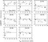 |
Fig. 12 Difference (LAMOST minus literature) between stellar labels estimated from the LAMOST R ~ 1800 spectra with HOTPAYNE and the literature values deduced from high-resolution spectroscopy for the reference stars, as a function of Teff. The symbols have the same meanings as in Fig. 11. The differences are likely dominated by the differences between the LTE (this study) and NLTE modeling. See the text for details. |
5.3 Teff and log g
Figure 13 presents the distribution of our sample stars with S /N > 30 in the Teff–log g diagram overplotted with the MIST stellar evolutionary tracks (Paxton et al. 2011; Choi et al. 2016), the numbers marked in red are the initial mass of the stellar evolutionary tracks. The majority of the sample stars have relatively cool temperatures, corresponding to stellar masses of 1.5–7.5 M⊙. While there are also a number of stars whose locations in the diagram are consistent with stellar mass higher than 20 M⊙. At the high-temperature end, there are a group of stars with log g > 5, which are outside the coverage of the stellar evolution tracks. These stars are mostly hot subdwarfs (e.g., sdBs and sdOs), whose origin is still a research topic (e.g., Webbink 1984; Han et al. 2002, 2003; Lanz et al. 2004; Miller Bertolami et al. 2008; Heber 2009; Justham et al. 2011; Zhang & Jeffery 2012). Hot subdwarfs have been extensively identified from the LAMOST database by Luo et al. (2016, 2019, Luo et al. 2020). The positions of the hot subdwarfs in the Teff–log g plane are consistent with Luo et al. (2016, e.g., see their Fig. 4), which is remarkable since our log g estimates for these stars are obtained via extrapolation of HOTPAYNE. Interestingly, Fig. 13 exhibits an upper border of the log g values that increase with Teff for the subdwarfs. A detailed study for the subdwarfs’ distribution morphology in the Teff-log g diagram is beyond the scope of this paper, but it deserves further dedicated work. It is also possible that a small number of these stars are “contamination” by unrecognized white dwarfs. Finally, we caution about the usage of our stellar labels for hot subdwarfs and white dwarfs, as they are estimated with model spectra that are extrapolations beyond the trained regime of HOTPAYNE.
At Teff ~ 10000 K (log Teff ~ 4), there is a vertical stripe of stars that extend to low log g values (<2). As we discuss further in Sect. 5.5, this is an artifact due to the existence of a large number of chemically peculiar stars, such as ApBp stars and Am stars. The log g of these stars may have been significantly underestimated as a consequence of masking the hydrogen lines for label determination for these early A-type and late B-type stars (Sect. 4.4). We note that such stars are prevalent in the hot-star regime; it is suggested that a high fraction of A-stars could be chemically peculiar (e.g., Gray et al. 2016; Qin et al. 2019; Xiang et al. 2020), and this is why their high number density constitutes a prominent stripe in the Teff-log g plane. Such an artifact reveals one of the limitations of the current model, which tends to yield incorrect log g for these chemically peculiar stars. However, as we show in Sect. 5.5, the abundance estimates of these stars are nonetheless robust enough, and thus these stars can be easily flagged through their abundance estimates.
About 98% of our sample stars have parallax measurements from the Gaia eDR3 (Gaia Collaboration 2021), which allow us to look into their luminosity (absolute magnitude). We derive their absolute magnitude in the 2MASS K-band (Skrutskie et al. 2006) using the distance modulus, adopting the Gaia eDR3 distance of Bailer-Jones et al. (2021). The interstellar extinction is corrected using the reddening E(B – V) interpolated from the 3D reddening map of Green et al. (2019) and a K-band extinction coefficient of 0.34 (e.g., Yuan et al. 2013). Figure 14 presents the stellar distribution in the Teff–MKs diagram for a subset of 195 879 stars with good spectral S/N (S /N > 30) and good parallax (ω/σω > 5). The figure illustrates a good correlation between MKs and log g, suggesting our log g estimates are robust for the overall sample stars. The figure also illustrates that at a given Teff, the vsin i exhibits little correlation with MKs. Finally, while relatively cool stars exhibit a wide range of vsin i values, the majority of hot stars with Teff > 25 000 K tend to exhibit large vsin i values (except for hot subdwarfs).
In Fig. 15 we show the (BP–RP) color of Gaia eDR3 as a function of our Teff estimates for stars with S /N > 30. There is a clear trend of (BP–RP) with Galactic latitude, which is due to the reddening effect. For stars at high Galactic latitude (|b| > 30°), there is a clear relation between Teff and (BP–RP), which is consistent well with the Teff-dependent trajectory of synthetic color from the MIST isochrones. Stars at low Galactic latitude exhibit a much broader (BP–RP) distribution, due to their large reddening effect. The right panel of Fig. 15 presents similar results, but correcting the color for interstellar reddening (BP–RP)0 estimated using the 3D reddening map of Green et al. (2019) and a total-to-selective extinction coefficient RBP = 3.24 and RRP = 1.91 (Chen et al. 2019). After de-reddening, the colors of the stars agree approximately with the expectation from the MIST isochrones. Interestingly, even after correcting for the reddening, a large fraction of hot stars with Teff > 25 000 K appear to be too red, with (BP–RP)0 ~ 0.0. These stars are likely either associated with star formation regions (for young stars) or have dust envelopes (for hot subdwarfs), as they suffer (locally) larger reddening than the Green et al. (2019) 3D “average” dust map (see also Xiang et al. 2021). The NLTE effects should push the temperature even higher than the current estimates and would only further exacerbate this discrepancy.
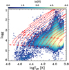 |
Fig. 13 Stellar number density distribution in the Kiel (Teff–log g) diagram. Only 211 245 stars with S /N > 30 are shown. Also shown in the figure are the MIST stellar evolution tracks (Paxton et al. 2011; Choi et al. 2016) with [Fe/H] = –0.5 and V/Vc = 0.4. The initial stellar masses of the tracks are marked (in unit of M⊙). The stars with log g > 5 and log Teff > 4.2 are hot subdwarfs. The vertical stripe at log Teff ~ 4.0 is an artifact for chemically peculiar stars (e.g., Ap/Bp stars and Am stars) whose log g have been underestimated as a consequence of masking the hydrogen lines for label determination. |
5.4 v sin i
The vsin i of our sample stars with S /N > 50 and log g < 5 are presented in Fig. 16. Here we adopt a stricter S/N cut than above for the Teff-log g plot (S /N > 30) to ensure the robustness of the vsin i for the stars presented in the figure. The vsin i estimates spread a broad range of values, from no rotation to faster than 600 km s−1. We note that our vsin i estimates could have negative values from the extrapolation of the model spectra beyond the well-trained regime of HOTPAYNE. A negative vsin i simply means that the star has little or no rotation. In the final catalog, we set all negative vsin i estimates to be 0 kms−1, but in Fig. 16 we keep the negative estimated values as they can serve as a good proxy for the uncertainties of the vsin i estimates. The extent of the negative tail suggests that the measurement uncertainties are on the order of 30 km s−1, which is in agreement with validation using the repeat observations (Fig. 10). We note that this number does not reflect any possible systematic errors. For stars of Teff < 10 000 K, the vsin i distribution peaks at ~30 km s−1, with a significant high-velocity tail extending to ~300km s−1, above which the number density free falls. The peak value shifts to slightly larger values for hotter stars, reaching ~50km s−1 for Teff > 16 000 K. This is qualitatively consistent with previous studies based on high-resolution spectroscopy, which have suggested that most of the early-type stars in the nearby Galactic disk rotate slower than 300km s−1, although a minor number of them can rotate faster than 400km s−1 (e.g., Abt et al. 2002; Huang et al. 2010; Bragança et al. 2012; Zorec & Royer 2012; Simón-Díaz & Herrero 2014; Li 2020).
Our results show that below 300 km s−1, the stellar number density exhibits a descending power-law. Abt et al. (2002) suggested that the vsin i distribution of late B-type (B8-B9.5 III-V) stars exhibits double peaks, contributed by a set of slow rotating chemically peculiar stars and a set of fast rotating normal stars (see also, e.g., Dufton et al. 2013). We examine this idea via the vsin i distribution for our sample stars in different Teff bins. The middle of the top-right panels of Fig. 16 presents the results for stars with 10000 < Teff < 16000 K, which are composed of late B-type stars. It shows a prominent peak of slow rotating stars at vsin i ~ 30 kms−1. While our results do not exhibit a clear double-peak feature, it indeed shows a significant tail of fast rotating stars (up to vsini ~ 300km s−1). The reason for the difference is unclear yet, and deserves to be further understood. This could be either because the relatively large measurement uncertainty of our estimates has smeared an intrinsic double-peak feature or because the intrinsic strength of the second peak is weaker than presented in previous work, particularly considering that the sample size in the literature is small (1/50 of the current sample). We note that vsin i estimates from medium-resolution (R = 7500) spectra of LAMOST for 40 034 early-type stars have recently become available (Sun et al. 2021). From this data set with better precision in vsini estimates, we confirmed the missing of a clear double-peak feature as found here. Independent of the temperature, our results show that slow rotators (<100kms−1) dominate over fast rotators for all stellar types from 7000 K (log Teff ~ 3.85) to 25000 K (log Teff ~ 4.4) (see the bottom-left panel of Fig. 16). The bottom-left panel of Fig. 16 also shows a significant fraction of slow rotators even above 25 000 K (log g > 4.4). This can also be seen in the right panel of Fig. 14, which displays numerous hot (Teff > 25 000 K), bright (MKs < 0) stars with vsini < 200km s−1.
The bottom-left panel of Fig. 16 illustrates that at the high-velocity end, the stellar density exhibits a sharp cutoff, and the cutoff velocity increases with Teff. The cutoff is particularly prominent for stars with Teff < 20 000 K (log Teff ~ 4.3), above which the cutoff becomes less well defined due to the sparsity of stars. Theoretically, a star cannot be formed with infinity rotation velocity because the rotation will induce centrifugal force, which increases with the rotation velocity. Once the centrifugal force is larger than the gravity, the rotating disk that accretes materials and angular momentum to sustain the star formation will break up. This causes an upper limit of the rotation velocity, which is referred as the critical velocity, or the break-up velocity (e.g., Maeder 2009). The critical velocity can be expressed as
 (7)
(7)
where G is gravity constant, M the stellar mass of a zero-age main-sequence (ZAMS) star, Rp the radius at the pole of the star. We assume that the Rp is approximately the same as the stellar radius in spherical models. In the bottom-left panel of Fig. 16, we show the critical velocity as a function of effective temperature. Here the critical velocity is derived using ZAMS stars with solar abundances. We retrieve the parameters (mass, Teff, and radius) of the ZAMS stars from the public MIST stellar isochrones (Paxton et al. 2011; Choi et al. 2016). Technically, for each Teff, we define the main-sequence star with the maximal log g as an approximation of the ZAMS star of that Teff.
It shows that, except for a few outliers, both the values and their Teff dependence of the observed vsin i border are consistent with the theoretical critical velocity, which increases from about 300km s−1 at Teff = 7000K to >600km s−1 at Teff = 40000K (log Teff ~ 4.6). This good agreement suggests that there are indeed a considerable fraction of stars rotating with a rate close to the critical velocity.
We note that some stars exhibit vsin i larger than the critical velocity. In principle, it is possible that a star might temporarily rotate faster than the critical velocity as a consequence of binary interaction (de Mink et al. 2013). However, upon inspecting the spectra and intrinsic brightness of these outliers, we find that they are mainly composed of nearly equal-brightness binary stars that exhibit large velocity difference between the individual components thus their spectral lines are broader than single stars. In addition, these outliers also include stars whose vsin i are erroneously estimated due to a number of reasons, such as the occurrence of strong emission lines, which is particularly common for O-type stars, the erroneously spectral radial velocity correction, the contamination of subdwarfs and white dwarfs, and the failure of the model spectra at the high-Teff end. For stars with Teff > 25 000 K, the inaccurate line strength of the Kurucz LTE model spectra may cause problems for the vsin i estimates. For example, by matching the He line profile of LAMOST with NLTE model spectra, Li (2020) suggests that LAMOST J040643.69+542347.8 (Teff ~ 35 000 K) has a vsin i of ~540kms−1, while our estimate is 261 ± 11 kms−1, significantly underestimated due to the poor reproduction of the spectral line profile by our LTE model spectra at such high Teff.
The bottom-right panel of Fig. 16 presents the relation between vsin i and [Fe/H]. While there is no strong trend between vsin i and [Fe/H] for the majority of stars, a small group of stars with vsin i ≲ 150kms−1 exhibit high metallicity ([Fe/H] ≳ 0.2). These stars are likely magnetic ApBp stars. We elaborate further on this point in the next section. On the metal-poor side, there is also an excess of stars with slow rotation velocities. These are found to be mostly BHB stars, presumably in the halo; due to their old age, they are rotating much more slowly than the typical young hot stars in the disk.
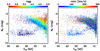 |
Fig. 14 Stellar distribution in the Teff–MKs diagram color-coded by log g (left) and vsin i (right). Only 194724 stars with good spectral S/N (S/N > 30) and good parallax (ω/σω > 5) are shown. The expected correlation between log g with MKs at a given Teff demonstrates the robustness of the spectroscopic log g estimates. The stars with Teff ≳ 20 000 K and MKs ~ 5 mag are hot subdwarfs. In the left panel, a maximal log g value of 5 is displayed in the color bar, and all stars with log g > 5 are shown with the same color as log g = 5 (dark blue). |
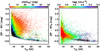 |
Fig. 15 Observed and de-reddened (BP–RP) color as a function of effective temperature. Only stars with spectral S/N > 30 are shown. The left panel shows the observed (BP–RP) color vs. Teff, with the stars color-coded by Galactic latitude as a rough proxy for the expected dust reddening. The gray line delineates the MIST isochrones’ prediction for (BP–RP) color as a function of Teff for ZAMS stars with initial [Fe/H] = 0. This panel illustrates that our sample stars in low Galactic latitudes suffer from a large reddening effect, leading to much redder colors than stars at high Galactic latitudes. The right panel shows (BP–RP)0, the de-reddened color, based on the 3D reddening map of Green et al. (2019), with the stars sorted and color-coded by log g. The panel illustrates that such de-reddened colors qualitatively agree with the isochrones, but the significant spread in color at any given temperature implies that the photometric colors alone would be too imprecise to estimate Teff robustly for stars above 10 000 K. The very hot stars with little reddening and very high log g are presumably near subdwarf B stars of modest luminosity (see Fig. 14). |
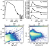 |
Fig. 16 Distribution of vsin i. Top left: histogram of vsin i for the overall sample in this work. Only results from stars with S /N > 50 and log g < 5 are shown. Top right: histogram of vsin i for stars in different Teff ranges, as marked in the figure. Bottom left: stellar number density distribution in the Teff-vsin i plane. The solid line delineates the critical rotation velocity, Vc, as a function of Teff, derived based on the ZAMS MIST isochrones (Choi et al. 2016). Bottom right: stellar number density distribution in the [Fe/H]–vsin i plane. Since we do not impose a prior limit on vsin i, our fit allows for negative vsin i values. A negative vsin i simply means that the star has a small rotation velocity, and the distribution at the negative tail serves as a proxy for the measurement uncertainties. |
5.5 Abundance [Fe/H] and [Si/H]
In light of the large systematics and uncertainties of our LTE-based abundance estimates, we opt to present only the [Fe/H] and [Si/H] in our catalog, while leaving the other abundances to future work. The [Fe/H] is an essential metallicity indicator for relatively cool stars (Teff < 10 000 K) both because the [Fe/H] of cool stars can have a broad range of values, as they come from different Galactic components (e.g., disk and halo), and because [Fe/H] can be robustly estimated for cool stars owing to their prominent features in the spectra. Silicon is a representative α-element. While the [Si/H] estimates may have large systematics (Fig. 12), we expect their relative values are robust and informative for identifying chemically peculiar stars (Fig. 17).
The left panel of Fig. 17 shows the stellar distribution in the Teff-[Fe/H] plane. A prominent feature in the figure is the v-shape pattern of [Fe/H] – typical [Fe/H] value for the bulk of stars decreases from –0.2 dex at the cool end (Teff ~ 7000 K) to a minimal value of about –0.7 dex at Teff ~ 17 000 K, beyond which the [Fe/H] slightly increases with Teff. This v-shape trend seems to be consistent with the high-resolution results of Gebruers et al. (2021). The origin of this trend is unclear. It is possibly an artifact due to NLTE effects. Beyond this trend, there is a group of stars with super-solar metallicity at Teff < 20 000 K, which are clearly separated from the bulk of stars in the [Fe/H]-Teff plane. For many of these Fe-rich stars, the [Si/H] are also significantly enhanced (see the right panel of Fig. 17). The high [Si/H] nature suggests these stars are likely chemically peculiar stars whose origin may be related to a strong magnetic field: magnetic ApBp stars (e.g., Abt et al. 1972, 2002; Preston 1974; Smith 1996; Mathys et al. 1997; Michaud et al. 2015; Hümmerich et al. 2020). These stars have been shown to be slow rotators with vsin i < 150kms−1 (Fig. 16), which is consistent with previous results (e.g., Abt et al. 2002; Preston 1974; Michaud et al. 2015). Besides the ApBp stars, our sample may also contain a significant number of other types of chemically peculiar stars (such as Hg-Mn stars, Am/Fm stars, He-deficient stars, etc.) as our sample stars are uniformly targeted without significant bias against any of these stars. Figure 17 shows that at the cool temperature side (Teff < 10 000 K), there is a large fraction of stars with super-solar metallicity, forming the high-[Fe/H] tail of the [Fe/H] distribution. Many of these super-solar metallicity stars are probably AmFm stars, which have been demonstrated to contributed a large fraction (~40%) of the A/F stars with mass higher than 1.4 M⊙ in the LAMOST sample (Xiang et al. 2020).
On the metal-poor side of the Teff–[Fe/H] plane, there is a significant number of metal-poor stars with [Fe/H] ≲ –1.0 dex, with a lower [Fe/H] border increasing from ~ –2.5 dex at Teff = 7000 K to ~ –1.5 dex at Teff = 11000 K. These metal-poor stars are mostly BHB stars and blue straggler stars of Galactic halo and thick disk populations; we expect there are very few single main-sequence stars given their high temperatures. As a demonstration, Fig. 18 shows that stars with  exhibit a [Fe/H] peak at around ~–1.6 dex, which is consistent with previous [Fe/H] estimates of the nearby halo stars (e.g., Carollo et al. 2007; Beers et al. 2012; An et al. 2013; Zuo et al. 2017; Youakim et al. 2020). It is expected that the nearby halo stars dominate our metal-poor sample as the majority of them are brighter than 14 mag (Fig. 2). Figure 18 shows that the BHB stars can be well separated from the blue stragglers in the Teff–log g diagram. The BHB stars in our sample can have a temperature higher than 10 000 K stars, and their distribution in the Teff–log g diagram is consistent with the prediction of the MIST evolutionary tracks. Whereas, blue stragglers, the product of binary mass transfer (Chen & Han 2008a,b), occupy a different locus in the Teff–log g plane as they have larger log g values than (and therefore are separable from) BHB. This makes it possible to identify a large set (~5000) of BHB stars (and blue straggler stars, as well), which have been widely used as tracers to study the structure and dynamics of the Milky Way halo (e.g., Sirko et al. 2004b,a; Kinman et al. 2007; Xue et al. 2008; De Propris et al. 2010; Ruhland et al. 2011; Kafle et al. 2012; Yang et al. 2019; Starkenburg et al. 2019; Bird et al. 2021), from the current sample.
Our results also reveal that most of these metal-poor stars are slow rotators with vsin i ≲ 150kms−1 (Fig. 16). Among them, we find that the BHB stars have a vsin i distribution of 49 ± 36 km s−1, which is qualitatively consistent with literature values (Peterson et al. 1995; Cohen & McCarthy 1997; Behr 2003; Recio-Blanco et al. 2004; Cortés et al. 2009), taking into account the relatively large uncertainty in our vsin i estimates.
The right panel of Fig. 17 illustrates that for the majority of stars of Teff > 8000 K, the [Si/H] estimates are consistent with the [Fe/H] estimates, while at the metal-poor side (e.g., [Fe/H] < –1.0 dex), the [Si/H] is about 0.2 dex higher than the [Fe/H], which means that the metal-poor halo stars have [Si/Fe] ~ 0.2 dex. This is consistent with the [α/Fe] values of the Galactic halo stars in previous work (e.g., Hayes et al. 2018; Conroy et al. 2019). We caution about the [Si/H] estimates for stars with Teff < 8000 K, which we find much larger uncertainties, probably due to the weak features of Si in those relatively cool stars.
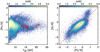 |
Fig. 17 Density distribution of our sample stars with S/N > 50 in the Teff – [Fe/H] (left) and [Fe/H] – [Si/H] (right) planes. In the left panel, the stars in red show the SPB stars of Gebruers et al. (2021), with [Fe/H] from high-resolution spectroscopy (LTE-based). While the Teff-dependent trend of the [Fe/H] distribution is likely due to NLTE effects, the figure clearly reveals the presence of chemically peculiar stars with super-solar [Fe/H] values, as well as halo BHB stars at the metal-poor end. The right panel shows good consistency between [Si/H] and [Fe/H], verifying the robustness of the determinations (regardless of the systematics due to NLTE). The group of stars with [Fe/H] ~ 0.7 dex and [Si/H] ≳ 1 dex are magnetic ApBp stars, as indicated by their signature enhancement in Si (e.g., Michaud et al. 2015). In the right panel, we omit stars with Teff < 8000 K because their [Si/H] estimates are found to suffer from larger systematics. |
5.6 The parameter catalog
Our stellar parameter catalog contains Teff, log g, vsin i, [Fe/H], and [Si/H] for 332172 unique stars with Teff > 7000 K and S /N > 5 from 454 693 spectra of LAMOST DR6. Among them, 59% are from both the LAMOST classification and the Zari et al. (2021) selection method; 29% are from the LAMOST classification only, and 11% are from the Zari et al. (2021) selection method only. Table 6 presents a description of the columns in our catalog. Here we summarize a few notes of caution when using the catalog.
First, for stars with log g > 5, which are mostly hot sub-dwarfs, the labels should be used with cautious as they are determined with model spectra extrapolated by HOTPAYNE. Second, we assigned a vsin i value of 0 km s−1 for stars for which our measurement gives negative values due to extrapolation. We also caution that although the vsin i estimates should be statistically robust, the uncertainty is large. An inspection of the spectra is necessary when focusing on the vsin i of individual stars, and this is particularly true for stars with unexpectedly large vsin i values as many of them have been found to be artifacts due to either binary effects or data imperfection.
Third, the labels are deduced based on LTE models. They may suffer systematics due to NLTE effects as well as stellar wind effects, particularly for stars with Teff > 25 000 K and for stars with low log g values.
Finally, the label uncertainties presented in the catalog are the formal errors of the fitting and have been scaled to match the dispersion of repeat observations as a function of Teff and S/N with a three-order polynomial, similar to in Xiang et al. (2019). The uncertainties provided here only concern the internal precision: they do not account for the zero-point offset induced by imperfections of the adopted model spectra.
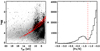 |
Fig. 18 Illustration of halo BHB stars revealed in the Teff–log g diagram. Left: Background in gray scale showing the stellar density (in logarithmic scale) of our sample stars with S/N > 50. The black dots represent the stars with |b| > 15° and [Fe/H] < –1.2 dex. There are two sequences separated in log g: the upper sequence with lower log g values is composed of halo BHB stars, and the lower sequence with larger log g values is presumed to comprise blue straggler stars. The solid lines in red are MIST evolutionary tracks of He-burning stars with [Fe/H] = –1.5, V/Vc = 0.4, and masses of 0.65, 0.60, and 0.58 M⊙, respectively, from upper to lower. The dashed lines in red show similar tracks but for [Fe/H] = –2.0. Right: [Fe/H] distribution of our sample stars with S/N > 50 and |b| > 15°. Only the metal-poor side of [Fe/H] < –0.5 dex is shown. The vertical dashed line indicates a constant [Fe/H] of –1.2 dex, the sample below which mostly comprises the metal-poor halo BHB stars. |
5.7 Future improvements
This is our first attempt at deriving stellar labels for hot stars from a vast set of low-resolution R ~ 1800 spectra, for which most of the spectral features are very blended and weak, with an automated full-spectral fitting technique. Although we have demonstrated that the R ~ 1800 optical spectra do contain a wealth of information of hot stars that in principle can give us robust estimates of stellar parameters as well as abundances for many (>5) elements, this work contains a few imperfections that need to be improved in future work.
First, it is well known that NLTE effects (and wind effects) play an important role for hot-star spectra. To obtain accurate labels, particularly for elemental abundances, a large grid of NLTE spectral models are urgently needed. Secondly, it is well known that a large fraction of hot stars are in binary systems (e.g., Sana et al. 2012, 2013; Xiang et al. 2021), future spec-troscopy should take the binary effect into account to derive reliable label estimates for binary systems. Similarly, many of the LAMOST O- and B-type stars (>10%) have emission lines in their spectra (e.g., Xiang et al. 2021). In the current work, we have neglected effects due to the emission lines. Therefore, for such systems, the stellar parameters might be problematic in unknown ways, adding uncertainty to stars hotter than 25 000 K. Thirdly, though in this work we have adopted the mean LSF of the LAMOST spectra, it is found that the fiber-to-fiber and temporal variations in the LAMOST LSF do have a significant impact on the vsin i estimates. Incorporating the exact LSF for individual stars should improve the vsin i measurements. Finally, we have adopted the stellar line-of-sight velocity from the LAMOST pipeline to correct the spectra into rest frame. However, we do find that, at times, the LAMOST pipeline provides erroneous line-of-sight velocities for some OB stars, particularly those with emission lines in their spectra. In future work, we may derive the stellar labels together with line-of-sight velocity simultaneously from the spectra.
6 Summary
In this study we have demonstrated that stellar atmospheric parameters and multiple elemental abundances of hot stars can be deduced from the low-resolution (R ~ 1800) optical spectra. This is first examined with the CR bound calculation, which suggests that for a typical B star with a spectral S/N of ~ 100, the theoretical limit of the precision one could attain is 300 K in Teff, 0.03 cms2 in logg, 1.0kms−1 in vmic, 10km s−1 in vsin i, 0.01 in NHe/Ntot, ~0.1 dex in abundances of C, O, Si, S, and Fe, and ~0.2 dex in abundances of N and Mg.
We adopted Payne to derive 11 labels – Teff, log g, vmic, vsin i, NHe/Ntot, [C/H], [N/H], [O/H], [Si/H], [S/H], and [Fe/H] – from a vast set of LAMOST spectra, taking the LTE-based Kurucz synthetic spectra as the underlying model spectra. Testing with synthetic spectra and examining with duplicate LAMOST observations confirms the robustness of the label estimates. We also show through the repeated spectra from the same objects that we can attain an internal precision that is consistent with the CR bound.
Despite the excellent internal precision and consistency, external examinations with literature values suggest that the abundance estimates may suffer non-negligible zero-point sys-tematics, likely consequences of NLTE effects. Nonetheless, the current estimates of Teff, log g, and vsin i are likely accurate, except for stars with Teff > 25000 K or supergiants with log g ≲ 2. Considering these nontrivial systematics, we present five stellar labels in our catalog, Teff, log g, vsin i, [Si/H], and [Fe/H], and can make other stellar labels available upon request.
In the Teff–log g diagram, our LAMOST sample stars cover a broad range of parameter space that corresponds to a stellar mass range from 1.5 M⊙ to larger than 50 M⊙. The vsin i distribution decreases roughly as a power law from a peak at ~30 kms−1 to ~300 km s−1, above which the stellar density exhibits a cutoff. This terminate vsin i increases with Teff, from ~300 km s−1 at 7000 K to ~600 kms−1 at 40 000 K. This Teff-dependent cutoff is consistent with the theoretical prediction of the critical rotation velocity. The vsin i distribution also suggests that at all temperature from 7000 to 25 000 K, the stars are dominated by slow rotators with vsin i < 100kms−1.
Our results reveal a sample of ApBp stars with significantly enhanced [Fe/H] ([Fe/H] > 0.2 dex) in the range of 7000 < Teff < 20000 K, and many of them also have significantly enhanced [Si/H] ([Si/H] > 0.4 dex). These ApBp stars have rotation velocities lower than 150kms−1, which is consistent with previous studies. The label estimates also allow the identification of a large sample of BHB stars in the Teff–log g plane. Our catalog of Teff, log g, vsin i, [Si/H], and [Fe/H] for a sample of 332 172 stars with Teff > 7000 K from LAMOST DR6, including more than 64 000 OB stars with Teff > 10 000 K, are publicly accessible.
Our analysis method and conclusion are generic and can be applied to other surveys, such as the SDSS-V survey. Future works based on NLTE analysis are desirable to improve upon the current results, particularly to obtain accurate stellar abundances from this vast set of LAMOST spectra, as well as the coming SDSS-V spectra.
Descriptions for the stellar label catalog of LAMOST DR6 hot stars.
Acknowledgements
The authors thank the reviewer, Prof. Artemio Herrero, for his carefully reading and valuable comments on the manuscripts. M. Xiang also thanks Prof. H.-W. Zhang for helpful discussion. Y.S.T. is grateful to be supported by the NASA Hubble Fellowship grant HST-HF2-51425.001 awarded by the Space Telescope Science Institute. R.P.K. acknowledges support by the Munich Excellence Cluster Origins funded under germany’s Excellence Strategy EXC-2094 390783311. S.G. gratefully acknowledges support from the Research Foundation Flanders (FWO) by means of a PhD Aspirant mandate under contract No. 11E5620N. The research leading to these results has (partially) received funding from the KU Leuven Research Council (grant C16/18/005: PARADISE), from the Research Foundation Flanders (FWO) under grant agreement G0H5416N (ERC Runner Up Project), and from the BELgian federal Science Policy Office (BELSPO) through PRODEX grant PLATO. This work has used data products from the Guoshoujing Telescope where the LAMOST survey was executed. LAMOST is a National Major Scientific Project built by the Chinese Academy of Sciences. Funding for the project has been provided by the National Development and Reform Commission. LAMOST is operated and managed by the National Astronomical Observatories, Chinese Academy of Sciences. This work has used data products from the European Space Agency (ESA) space mission Gaia. Gaia data are being processed by the Gaia Data Processing and Analysis Consortium (DPAC). Funding for the DPAC is provided by national institutions, in particular the institutions participating in the Gaia MultiLateral Agreement. The Gaia mission website is https://www.cosmos.esa.int/gaia. The Gaia archive website is https://archives.esac.esa.int/gaia. This work has used the ESO archive data, with the following project ids: 60.A-9022, 70.D-0191, 072.C-0488, 076.B-0055, 077.C-0379, 084.B-0869, 095.D-0234, 096.D-0008, 0101.C-0360, 0102.C-0124, 183.C-0972, 194.C-0833. This work has used data products from the 2MASS, which is a joint project of the University of Massachusetts and the Infrared Processing and Analysis Center/California Institute of Technology, funded by the National Aeronautics and Space Administration and the National Science Foundation. This work has used the CDS-Xmatch service (http://cdsxmatch.u-strasbg.fr/xmatch). This work has also used the TOPCAT, IDL and Python software infrastructure.
Appendix A The gradient spectra of early A-type stars
The A0-type dwarfs have the strongest hydrogen lines in their spectra, which means that the gradient spectra ∂fλ/∂λ of hydrogen lines reach a minimum for these stars. As an illustration, Fig. A.1 shows the gradient spectra of dwarf stars (log g = 4.5, [Fe/H] = 0) at different temperatures. The gradient spectra of hydrogen lines have negative values at Teff < 9500 K, and become positive values at Teff > 9500 K. This reversal leads to the A0 “desert” shown in Fig. 9.
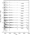 |
Fig. A.1 Gradient spectra of Teff derived from the Kurucz model at different effective temperatures, as marked in the figure. We assume log g = 4.5 and [Fe/H] = 0. The A0 dwarf (Teff = 9500 K) has the minimal gradients in hydrogen lines (close to 0), and they form an inflection point in the gradient of the hydrogen lines as a function of Teff, which leads to the artificial A0 star desert of the stellar distribution in the Teff-log g diagram as seen in Fig. 9. |
Appendix B The Cramér-Rao bound of A stars
Figure B.1 shows the CR bound for an A-type dwarf star with Teff = 9500 K, log g = 4, and [Fe/H] = 0, both from the full (unmasked) spectra and from the spectra after masking hydrogen lines as introduced in Sect. 4.5. Masking hydrogen lines loses part of the astrophysical information content, thereby increasing the CR bound. Nevertheless, the label estimates remain feasible even after applying the masking, with CR bounds of ~100K in Teff, 0.1 dex in log g, 0.3 km s−1 in vmic, 15 km s−1 in vsin i, and 0.1 dex in the abundance for a few elements (e.g., C, O, Mg, Fe) for a spectral S/N of 100.
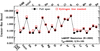 |
Fig. B.1 CR bound for an A-type star with Teff = 9500 K, log g = 4.5, and [Fe/H] = 0. The black dots show the CR bound derived from the full spectra, and the red squares are derived from the spectra after masking the hydrogen lines as described in Sect. 4.5. |
Appendix C Comparison between LTE and NLTE model spectra
Figures C.1 and C.2 present a comparison of the Kurucz LTE model spectra with NLTE spectra from the Potsdam Wolf-Rayet (PoWR) models (Hainich et al. 2019), for different temperatures. The NLTE effects (and stellar winds) strongly impact the helium lines at all temperatures, and have strong impacts on the hydrogen lines for stars with Teff ≳ 25 000 K (see also, e.g., Auer & Mihalas 1972; Kudritzki 1976, 1979).
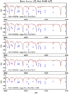 |
Fig. C.1 Comparison of Kurucz LTE model spectra (black) with the PoWR NLTE model spectra (red) for different parameters. The NLTE effect has a strong impact on the He lines and metal lines at all temperatures, and it also has a strong impact on the hydrogen lines for stars with Teff ≳ 25 000 K. |
References
- Abt, H. A., Chaffee, F. H., & Suffolk, G. 1972, ApJ, 175, 779 [NASA ADS] [CrossRef] [Google Scholar]
- Abt, H. A., Levato, H., & Grosso, M. 2002, ApJ, 573, 359 [NASA ADS] [CrossRef] [Google Scholar]
- Aerts, C. 2021, Rev. Mod. Phys., 93, 015001 [Google Scholar]
- Ahumada, R., Prieto, C. A., Almeida, A., et al. 2020, ApJS, 249, 3 [Google Scholar]
- An, D., Beers, T. C., Johnson, J. A., et al. 2013, ApJ, 763, 65 [NASA ADS] [CrossRef] [Google Scholar]
- Asplund, M., Grevesse, N., Sauval, A. J., & Scott, P. 2009, ARA&A, 47, 481 [NASA ADS] [CrossRef] [Google Scholar]
- Auer, L. H., & Mihalas, D. 1972, ApJS, 24, 193 [NASA ADS] [CrossRef] [Google Scholar]
- Bailer-Jones, C. A. L., Rybizki, J., Fouesneau, M., Demleitner, M., & Andrae, R. 2021, AJ, 161, 147 [Google Scholar]
- Beers, T. C., Carollo, D., Ivezić, Ž., et al. 2012, ApJ, 746, 34 [NASA ADS] [CrossRef] [Google Scholar]
- Behr, B. B. 2003, ApJS, 149, 101 [NASA ADS] [CrossRef] [Google Scholar]
- Berger, T. A., Kudritzki, R.-P., Urbaneja, M. A., et al. 2018, ApJ, 860, 130 [CrossRef] [Google Scholar]
- Bird, S. A., Xue, X.-X., Liu, C., et al. 2021, ApJ, 919, 66 [NASA ADS] [CrossRef] [Google Scholar]
- Boch, T., Pineau, F., & Derriere, S. 2012, ASP Conf. Ser., 461, 291 [NASA ADS] [Google Scholar]
- Borucki, W. J., Koch, D., Basri, G., et al. 2010, Science, 327, 977 [Google Scholar]
- Bragança, G. A., Daflon, S., Cunha, K., et al. 2012, AJ, 144, 130 [CrossRef] [Google Scholar]
- Buder, S., Sharma, S., Kos, J., et al. 2021, MNRAS, 506, 150 [NASA ADS] [CrossRef] [Google Scholar]
- Carlin, J. L., Lépine, S., Newberg, H. J., et al. 2012, Res. Astron. Astrophys., 12, 755 [CrossRef] [Google Scholar]
- Carollo, D., Beers, T. C., Lee, Y. S., et al. 2007, Nature, 450, 1020 [NASA ADS] [CrossRef] [Google Scholar]
- Casey, A. R., Hawkins, K., Hogg, D. W., et al. 2017, ApJ, 840, 59 [NASA ADS] [CrossRef] [Google Scholar]
- Chen, X., & Han, Z. 2008a, MNRAS, 384, 1263 [Google Scholar]
- Chen, X., & Han, Z. 2008b, MNRAS, 387, 1416 [NASA ADS] [CrossRef] [Google Scholar]
- Chen, B. Q., Liu, X. W., Yuan, H. B., et al. 2018, MNRAS, 476, 3278 [NASA ADS] [CrossRef] [Google Scholar]
- Chen, B. Q., Huang, Y., Yuan, H. B., et al. 2019, MNRAS, 483, 4277 [Google Scholar]
- Choi, J., Dotter, A., Conroy, C., et al. 2016, ApJ, 823, 102 [Google Scholar]
- Chojnowski, S. D., Hubrig, S., Hasselquist, S., et al. 2020, MNRAS, 496, 832 [NASA ADS] [CrossRef] [Google Scholar]
- Cohen, J. G., & McCarthy, J. K. 1997, AJ, 113, 1353 [NASA ADS] [CrossRef] [Google Scholar]
- Conroy, C., Naidu, R. P., Zaritsky, D., et al. 2019, ApJ, 887, 237 [NASA ADS] [CrossRef] [Google Scholar]
- Cortés, C., Silva, J. R. P., Recio-Blanco, A., et al. 2009, ApJ, 704, 750 [CrossRef] [Google Scholar]
- Cramér, H. 1945, Mathematical Methods of Statistics (Princeton: Princeton University Press) [Google Scholar]
- Cui, X.-Q., Zhao, Y.-H., Chu, Y.-Q., et al. 2012, Res. Astron. Astrophys., 12, 1197 [Google Scholar]
- De Cat, P., Fu, J. N., Ren, A. B., et al. 2015, ApJS, 220, 19 [NASA ADS] [CrossRef] [Google Scholar]
- de Mink, S. E., Langer, N., Izzard, R. G., Sana, H., & de Koter, A. 2013, ApJ, 764, 166 [Google Scholar]
- Deng, L.-C., Newberg, H. J., Liu, C., et al. 2012, Res. Astron. Astrophys., 12, 735 [Google Scholar]
- De Propris, R., Harrison, C. D., & Mares, P. J. 2010, ApJ, 719, 1582 [NASA ADS] [CrossRef] [Google Scholar]
- Dotter, A. 2016, ApJS, 222, 8 [Google Scholar]
- Dufton, P. L., Langer, N., Dunstall, P. R., et al. 2013, A&A, 550, A109 [NASA ADS] [CrossRef] [EDP Sciences] [Google Scholar]
- Ekström, S., Georgy, C., Eggenberger, P., et al. 2012, A&A, 537, A146 [Google Scholar]
- Fu, J.-N., Cat, P. D., Zong, W., et al. 2020, Res. Astron. Astrophys., 20, 167 [CrossRef] [Google Scholar]
- Gaia Collaboration ( Brown, A.G.A., et al.) 2018, A&A, 616, A1 [NASA ADS] [CrossRef] [EDP Sciences] [Google Scholar]
- Gaia Collaboration ( Brown, A.G.A., et al.) 2021, A&A, 649, A1 [NASA ADS] [CrossRef] [EDP Sciences] [Google Scholar]
- García Pérez, A. E., Allende Prieto, C., Holtzman, J. A., et al. 2016, AJ, 151, 144 [Google Scholar]
- Gebran, M., Monier, R., Royer, F., Lobel, A., & Blomme, R. 2014, in Putting A Stars into Context: Evolution, Environment, and Related Stars, eds. G. Mathys, E.R. Griffin, O. Kochukhov, R. Monier, & G.M. Wahlgren, 193 [Google Scholar]
- Gebruers, S., Straumit, I., Tkachenko, A., et al. 2021, A&A, 650, A151 [NASA ADS] [CrossRef] [EDP Sciences] [Google Scholar]
- Gray, D. F. 1992, The Observation and Analysis of Stellar Photospheres (Cambridge: Cambridge University Press), 20 [Google Scholar]
- Gray, R. O., Corbally, C. J., De Cat, P., et al. 2016, AJ, 151, 13 [Google Scholar]
- Green, G. M., Schlafly, E., Zucker, C., Speagle, J. S., & Finkbeiner, D. 2019, ApJ, 887, 93 [NASA ADS] [CrossRef] [Google Scholar]
- Hainich, R., Ramachandran, V., Shenar, T., et al. 2019, A&A, 621, A85 [NASA ADS] [CrossRef] [EDP Sciences] [Google Scholar]
- Han, Z., Podsiadlowski, P., Maxted, P. F. L., Marsh, T. R., & Ivanova, N. 2002, MNRAS, 336, 449 [Google Scholar]
- Han, Z., Podsiadlowski, P., Maxted, P. F. L., & Marsh, T. R. 2003, MNRAS, 341, 669 [NASA ADS] [CrossRef] [Google Scholar]
- Haucke, M., Cidale, L. S., Venero, R. O. J., et al. 2018, A&A, 614, A91 [NASA ADS] [CrossRef] [EDP Sciences] [Google Scholar]
- Hayes, C. R., Majewski, S. R., Shetrone, M., et al. 2018, ApJ, 852, 49 [NASA ADS] [CrossRef] [Google Scholar]
- Heber, U. 2009, ARA&A, 47, 211 [Google Scholar]
- Ho, A. Y. Q., Ness, M. K., Hogg, D. W., et al. 2017, ApJ, 836, 5 [NASA ADS] [CrossRef] [Google Scholar]
- Hoaglin, D. C., Mosteller, F., & Tukey, J. W. 1983, Understanding Robust and Exploratory Data Anlysis (Hoboken: John Wiley & Sons) [Google Scholar]
- Hobbs, L. M., York, D. G., Snow, T.P., et al. 2008, ApJ, 680, 1256 [NASA ADS] [CrossRef] [Google Scholar]
- Holgado, G., Simon-Diaz, S., Barba, R. H., et al. 2018, A&A, 613, A65 [NASA ADS] [CrossRef] [EDP Sciences] [Google Scholar]
- Huang, W., Gies, D.R., & McSwain, M.V. 2010, ApJ, 722, 605 [NASA ADS] [CrossRef] [Google Scholar]
- Hubeny, I., & Lanz, T. 1995, ApJ, 439, 875 [Google Scholar]
- Hubeny, I., & Lanz, T. 2011, Astrophysics Source Code Library [record ascl:1109.022] [Google Scholar]
- Hümmerich, S., Paunzen, E., & Bernhard, K. 2020, A&A, 640, A40 [NASA ADS] [CrossRef] [EDP Sciences] [Google Scholar]
- Jorgensen, U. G., Larsson, M., Iwamae, A., & Yu, B. 1996, A&A, 315, 204 [NASA ADS] [Google Scholar]
- Justham, S., Podsiadlowski, P., & Han, Z. 2011, MNRAS, 410, 984 [CrossRef] [Google Scholar]
- Kafle, P. R., Sharma, S., Lewis, G. F., & Bland-Hawthorn, J. 2012, ApJ, 761, 98 [NASA ADS] [CrossRef] [Google Scholar]
- Kingma, D. P., & Ba, J. 2014, ArXiv e-prints [arXiv:1412.6980] [Google Scholar]
- Kinman, T. D., Cacciari, C., Bragaglia, A., Buzzoni, A., & Spagna, A. 2007, MNRAS, 375, 1381 [NASA ADS] [CrossRef] [Google Scholar]
- Kollmeier, J. A., Zasowski, G., Rix, H.-W., et al. 2017, ArXiv e-prints [arXiv:1711.03234] [Google Scholar]
- Kudritzki, R. P. 1976, A&A, 52, 11 [NASA ADS] [Google Scholar]
- Kudritzki, R. P. 1979, Liege International Astrophysical Colloquia, 22, 295 [NASA ADS] [Google Scholar]
- Kudritzki, R. P. 1998, in Stellar astrophysics for the local group: VIII Canary Islands Winter School of Astrophysics, eds. A. Aparicio, A. Herrero, & F. Sanchez, 149 [Google Scholar]
- Kudritzki, R.-P., & Puls, J. 2000, ARA&A, 38, 613 [Google Scholar]
- Kudritzki, R. P., Castro, N., Urbaneja, M. A., et al. 2016, ApJ, 829, 70 [NASA ADS] [CrossRef] [Google Scholar]
- Kurucz, R. L. 1970, SAO Special Report, 309 [Google Scholar]
- Kurucz, R. L. 1993, SYNTHE Spectrum Synthesis Programs and Line Data (Cambridge, Mass.: Smithsonian Astrophysical Observatory) [Google Scholar]
- Kurucz, R. L. 2005, Mem. Soc. Astron. It. Suppl., 8, 14 [Google Scholar]
- Lanz, T., & Hubeny, I. 2007, ApJS, 169, 83 [CrossRef] [Google Scholar]
- Lanz, T., Brown, T. M., Sweigart, A. V., Hubeny, I., & Landsman, W. B. 2004, ApJ, 602, 342 [CrossRef] [Google Scholar]
- Lee, Y. S., Beers, T. C., Sivarani, T., et al. 2008, AJ, 136, 2022 [Google Scholar]
- Li, G.-W. 2020, ApJ, 892, L26 [NASA ADS] [CrossRef] [Google Scholar]
- Liu, X. W., Yuan, H. B., Huo, Z. Y., et al. 2014, IAU Symp., 298, 310 [NASA ADS] [Google Scholar]
- Liu, Z., Cui, W., Liu, C., et al. 2019, ApJS, 241, 32 [CrossRef] [Google Scholar]
- Luo, A. L., Zhao, Y.-H., Zhao, G., et al. 2015, Res. Astron. Astrophys., 15, 1095 [Google Scholar]
- Luo, Y.-P., Németh, P., Liu, C., Deng, L.-C., & Han, Z.-W. 2016, ApJ, 818, 202 [NASA ADS] [CrossRef] [Google Scholar]
- Luo, Y., Németh, P., Deng, L., & Han, Z. 2019, ApJ, 881, 7 [NASA ADS] [CrossRef] [Google Scholar]
- Luo, Y., Németh, P., & Li, Q. 2020, ApJ, 898, 64 [Google Scholar]
- Maeder, A. 2009, Physics, Formation and Evolution of Rotating Stars (Berlin: Springer) [Google Scholar]
- Maeder, A., Przybilla, N., Nieva, M.-F., et al. 2014, A&A, 565, A39 [NASA ADS] [CrossRef] [EDP Sciences] [Google Scholar]
- Martins, F., Hervé, A., Bouret, J. C., et al. 2015, A&A, 575, A34 [NASA ADS] [CrossRef] [EDP Sciences] [Google Scholar]
- Masseron, T., Plez, B., Van Eck, S., et al. 2014, A&A, 571, A47 [NASA ADS] [CrossRef] [EDP Sciences] [Google Scholar]
- Mathys, G., Hubrig, S., Landstreet, J. D., Lanz, T., & Manfroid, J. 1997, A&AS, 123, 353 [NASA ADS] [CrossRef] [EDP Sciences] [Google Scholar]
- Michaud, G., Alecian, G., & Richer, J. 2015, Atomic Diffusion in Stars (Berlin: Springer) [Google Scholar]
- Miller Bertolami, M. M., Althaus, L. G., Unglaub, K., & Weiss, A. 2008, A&A, 491, 253 [NASA ADS] [CrossRef] [EDP Sciences] [Google Scholar]
- Nieva, M. F., & Przybilla, N. 2012, A&A, 539, A143 [NASA ADS] [CrossRef] [EDP Sciences] [Google Scholar]
- Nieva, M.-F., & Przybilla, N. 2014, A&A, 566, A7 [NASA ADS] [CrossRef] [EDP Sciences] [Google Scholar]
- Paunzen, E., Hümmerich, S., & Bernhard, K. 2021, A&A, 645, A34 [NASA ADS] [CrossRef] [EDP Sciences] [Google Scholar]
- Paxton, B., Bildsten, L., Dotter, A., et al. 2011, ApJS, 192, 3 [Google Scholar]
- Pedersen, M. G., Aerts, C., Papics, P. I., & Rogers, T. M. 2018, A&A, 614, A128 [NASA ADS] [CrossRef] [EDP Sciences] [Google Scholar]
- Peterson, R. C., Rood, R. T., & Crocker, D. A. 1995, ApJ, 453, 214 [NASA ADS] [CrossRef] [Google Scholar]
- Preston, G. W. 1974, ARA&A, 12, 257 [Google Scholar]
- Przybilla, N., Butler, K., Becker, S. R., & Kudritzki, R. P. 2006, A&A, 445, 1099 [NASA ADS] [CrossRef] [EDP Sciences] [Google Scholar]
- Przybilla, N., Nieva, M.-F., & Butler, K. 2008, ApJ, 688, L103 [CrossRef] [Google Scholar]
- Przybilla, N., Firnstein, M., Nieva, M. F., Meynet, G., & Maeder, A. 2010, A&A, 517, A38 [NASA ADS] [CrossRef] [EDP Sciences] [Google Scholar]
- Qin, L., Luo, A. L., Hou, W., et al. 2019, ApJS, 242, 13 [NASA ADS] [CrossRef] [Google Scholar]
- Rao, C. R. 1945, Bull. Calcutta Math. Soc., 37, 81 [Google Scholar]
- Recio-Blanco, A., Piotto, G., Aparicio, A., & Renzini, A. 2004, A&A, 417, 597 [NASA ADS] [CrossRef] [EDP Sciences] [Google Scholar]
- Renson, P., & Manfroid, J. 2009, A&A, 498, 961 [NASA ADS] [CrossRef] [EDP Sciences] [Google Scholar]
- Ruhland, C., Bell, E. F., Rix, H.-W., & Xue, X.-X. 2011, ApJ, 731, 119 [NASA ADS] [CrossRef] [Google Scholar]
- Rybizki, J., Green, G., Rix, H.-W., et al. 2022, MNRAS, 510, 2597 [NASA ADS] [CrossRef] [Google Scholar]
- Sana, H., de Mink, S. E., de Koter, A., et al. 2012, Science, 337, 444 [Google Scholar]
- Sana, H., de Koter, A., de Mink, S. E., et al. 2013, A&A, 550, A107 [NASA ADS] [CrossRef] [EDP Sciences] [Google Scholar]
- Sandford, N. R., Weisz, D. R., & Ting, Y.-S. 2020, ApJS, 249, 24 [NASA ADS] [CrossRef] [Google Scholar]
- Simón-Díaz, S., & Herrero, A. 2014, A&A, 562, A135 [NASA ADS] [CrossRef] [EDP Sciences] [Google Scholar]
- Sirko, E., Goodman, J., Knapp, G. R., et al. 2004a, AJ, 127, 899 [NASA ADS] [CrossRef] [Google Scholar]
- Sirko, E., Goodman, J., Knapp, G. R., et al. 2004b, AJ, 127, 914 [NASA ADS] [CrossRef] [Google Scholar]
- Skrutskie, M. F., Cutri, R. M., Stiening, R., et al. 2006, AJ, 131, 1163 [NASA ADS] [CrossRef] [Google Scholar]
- Smith, K. C. 1996, Ap&SS, 237, 77 [NASA ADS] [CrossRef] [Google Scholar]
- Starkenburg, E., Youakim, K., Martin, N., et al. 2019, MNRAS, 490, 5757 [Google Scholar]
- Steinmetz, M., Guiglion, G., McMillan, P. J., et al. 2020, AJ, 160, 83 [NASA ADS] [CrossRef] [Google Scholar]
- Sun, W., Duan, X.-W., Deng, L., et al. 2021, ApJS, 257, 22 [NASA ADS] [CrossRef] [Google Scholar]
- Takeda, Y., Kawanomoto, S., & Ohishi, N. 2007, PASJ, 59, 245 [NASA ADS] [CrossRef] [Google Scholar]
- Talon, S., Richard, O., & Michaud, G. 2006, ApJ, 645, 634 [Google Scholar]
- Ting, Y.-S., Conroy, C., & Rix, H.-W. 2016, ApJ, 826, 83 [NASA ADS] [CrossRef] [Google Scholar]
- Ting, Y.-S., Conroy, C., Rix, H.-W., & Cargile, P. 2017a, ApJ, 843, 32 [NASA ADS] [CrossRef] [Google Scholar]
- Ting, Y.-S., Rix, H.-W., Conroy, C., Ho, A. Y. Q., & Lin, J. 2017b, ApJ, 849, L9 [NASA ADS] [CrossRef] [Google Scholar]
- Ting, Y.-S., Conroy, C., Rix, H.-W., & Cargile, P. 2019, ApJ, 879, 69 [Google Scholar]
- Vick, M., Michaud, G., Richer, J., & Richard, O. 2010, A&A, 521, A62 [EDP Sciences] [Google Scholar]
- Webbink, R. F. 1984, ApJ, 277, 355 [NASA ADS] [CrossRef] [Google Scholar]
- Xiang, M. S., Liu, X. W., Yuan, H. B., et al. 2015, MNRAS, 448, 822 [NASA ADS] [CrossRef] [Google Scholar]
- Xiang, M. S., Liu, X. W., Yuan, H. B., et al. 2017, MNRAS, 467, 1890 [NASA ADS] [Google Scholar]
- Xiang, M., Ting, Y.-S., Rix, H.-W., et al. 2019, ApJS, 245, 34 [Google Scholar]
- Xiang, M.-S., Rix, H.-W., Ting, Y.-S., et al. 2020, ApJ, 898, 28 [Google Scholar]
- Xiang, M., Rix, H.-W., Ting, Y.-S., et al. 2021, ApJS, 253, 22 [NASA ADS] [CrossRef] [Google Scholar]
- Xue, X. X., Rix, H. W., Zhao, G., et al. 2008, ApJ, 684, 1143 [Google Scholar]
- Yang, C., Xue, X.-X., Li, J., et al. 2019, ApJ, 886, 154 [NASA ADS] [CrossRef] [Google Scholar]
- Youakim, K., Starkenburg, E., Martin, N. F., et al. 2020, MNRAS, 492, 4986 [CrossRef] [Google Scholar]
- Yuan, H. B., Liu, X. W., & Xiang, M. S. 2013, MNRAS, 430, 2188 [NASA ADS] [CrossRef] [Google Scholar]
- Yuan, H. B., Liu, X. W., Huo, Z. Y., et al. 2015, MNRAS, 448, 855 [NASA ADS] [CrossRef] [Google Scholar]
- Zari, E., Rix, H. W., Frankel, N., et al. 2021, A&A, 650, A112 [NASA ADS] [CrossRef] [EDP Sciences] [Google Scholar]
- Zhang, X., & Jeffery, C. S. 2012, MNRAS, 419, 452 [NASA ADS] [CrossRef] [Google Scholar]
- Zhao, G., Zhao, Y.-H., Chu, Y.-Q., Jing, Y.-P., & Deng, L.-C. 2012, Res. Astron. Astrophys., 12, 723 [NASA ADS] [CrossRef] [Google Scholar]
- Zorec, J., & Royer, F. 2012, A&A, 537, A120 [NASA ADS] [CrossRef] [EDP Sciences] [Google Scholar]
- Zuo, W., Du, C., Jing, Y., et al. 2017, ApJ, 841, 59 [NASA ADS] [CrossRef] [Google Scholar]
Since those with  and
and  and
and  and
and  are likely affected by imperfect initial Teff estimates from the line indices. For those objects, we opted to redetermine their full-spectra-based labels using the H-masked Teff as the initial estimates.
Stellar variability could be an issue as well, but we do not expect it to dominate over the measurement uncertainties for the majority of stars.
[Si/H] is presented as a representative α-element. As we show in Sect. 5.5, despite the systematics due to the NLTE effects, the [Si/H] estimates are still informative at least for chemically peculiar stars.
The dispersion is defined as a resistant estimate of the standard deviation, adopting the robust_sigma.pro in the IDL astronomical library. See, for instance, Hoaglin et al. (1983) for the method of resistant estimate of the dispersion of a distribution.
All Tables
Elemental abundances of our reference stars from NLTE analyses of high-resolution spectra.
All Figures
|
Fig. 1 On-sky distribution of our LAMOST DR6 hot-star candidates in Galactic coordinates (l, b). The map is centered on the Galactic anticenter (l = 180°, b = 0°). The thick line delineates the celestial equator (Dec = 0°), and lines of constant declination, Dec = ±30° and Dec = ±60°, are also shown. Colors indicate the logarithmic number of stars in each (l, b) cell of 0.2° × 0.2°. The distribution reflects both the LAMOST survey area and the candidate stars’ concentration to the Galactic plane, which is expected for young stars. |
| In the text | |
|
Fig. 2 Distribution of our LAMOST DR6 hot-star candidates in the Gaia G-band magnitude and LAMOST spectral S/N plane. The G-band magnitudes cover a dynamic range of nearly 15 magnitudes, and most of them are between G ~ 10 and 18 mag. The spectral S/N peaks at around 63 (log(S /N) ~ 1.8) but has a median value of 37 due to a significant low-S/N tail. The isodensity contours encompass 68.3, 95, and 99.7% of the sample stars, respectively, and the colors delineate the relative stellar number density, with darker colors representing higher density. |
| In the text | |
|
Fig. 3 Information content of low-resolution spectra for a B star. Each panel shows the gradient spectrum ∇l : = ∂fλ/∂l with respect to different labels, l, derived from finite differencing of Kurucz model spectra (black) at Teff = 18 000 K, log g = 4.0, [Fe/H] = 0, and vsin i = 100 km s−1. The gradient spectra generated from HOTPAYNE are overplotted in red, illustrating the robustness of HOTPAYNE: the good agreement to the Kurucz model suggests that HOTPAYNE determines the labels from the relevant features instead of harnessing the astrophysical correlations. For Teff, vmic, vsin i, and NHe/Ntot, the gradient spectra are multiplied by 1000 K in Teff, 5 km s−1 in vmic, 20 km s−1 in vsin i, and 0.05 in NHe/Ntot for better visibility. This figure shows that the diagnostic signatures of label changes are widely distributed across the optical spectral range. Nonetheless, most spectral features are subtle due to LAMOST’s spectral resolution and the high effective temperature of the star: most abundance signatures are at the 1% level, even for abundance changes of 1 dex. Useful information about hot stars can only be extracted from a global fit to the spectrum and a careful spectral modeling. |
| In the text | |
|
Fig. 4 Theoretical precision limits for stellar label determination from LAMOST of hot stars, expressed through the CR bound, |
| In the text | |
|
Fig. 5 Correlation coefficients among the stellar label estimates, predicted by the CR bound calculation (see Eq. (3)). These correlations were derived for the spectrum of a fiducial B-type star with Teff = 18 000 K, log g = 4.0, [Fe/H] = 0, and vsin i = 100 kms−1. Prominent among the correlations are those between estimates of Teff and log g, and between NHe/Ntot and both Teff and log g. The nontrivial correlations suggest that most spectral features are somewhat blended and thus call for a simultaneous fit of all pertinent labels to the entire spectrum. |
| In the text | |
|
Fig. 6 Precision of the spectrum prediction by HOTPAYNE, which entails a neural-net-enabled interpolation among Kurucz model spectra. The left panels show the comparison between the Kurucz spectrum and its prediction by HOTPAYNE for a test star with Teff = 18 236 K, log g = 4.23, and [Fe/H] = 0.0. Top-right panel: distribution of flux residuals for all of our 1012 test spectra, each with 3801 pixels in the wavelength range of λλ3750–9000 Å. A Gaussian fit to the distribution yields a standard deviation of 0.165%. Bottom-right panel: analogous to the top-right panel, but only for pixels whose normalized spectral fluxes are smaller than 0.95, i.e., for strong absorption lines, mostly the cores of H and He lines. The standard deviation from a Gaussian fit is 0.586% for the strong absorption features. |
| In the text | |
|
Fig. 7 Precision of the HOTPAYNE label estimates as a function of Teff. Plotted are the differences (residuals) between the labels from HOTPAYNE and the true values for a test set of Kurucz model spectra with S/N ~ 100, color-coded by the true values. The numbers marked in the figure are the dispersion derived from a Gaussian fit to the residuals. The precision of the HOTPAYNE label determination varies with Teff and [X/H]. For metal-poor stars of [X/H] < −1 dex, the [X/H] estimates may suffer large uncertainties. However, we note that in the real case of the LAMOST survey, we do not expect there to be many hot stars with such low metallicities. |
| In the text | |
|
Fig. 8 Example of the HotPayne fit for a B-type star (top) and an early A-type star (bottom). The LAMOST spectra are shown in black, and the best-fit HotPayne models are shown in red. The masked telluric bands, the DIB, the interstellar absorption of Na and Ca, and the dichroic region are marked by shaded regions. For the case of early A-type stars, the wavelength windows of hydrogen lines (Balmer and Paschen series) are also masked (see text). |
| In the text | |
|
Fig. 9 Teff-log g diagrams for Teff derived from the LAMOST spectra without (left) and with (middle) the hydrogen lines masked. Right panel: direct comparison of the Teff estimates in the left and middle panels. The inclusion of hydrogen lines for the label determination causes an artificial desert of early A-type (and late B-type) dwarf stars in the Teff-log g diagram due to the reverse of spectral gradients |
| In the text | |
|
Fig. 10 Label differences between repeat observations as a function of S/N for stars with Teff > 10 000 K. Only repeat observations carried out on different observation nights and with S/N differences of less than 20 percent are adopted. The x axis shows the mean S/N of the repeat observations. The solid lines in red show the median differences as well as the standard deviations at different S/N. The numbers marked in the figure are precision (the scatter divided by |
| In the text | |
|
Fig. 11 Comparison of labels between the HOTPAYNE estimates and high-resolution spectroscopic results for our reference stars. For all the dots in black, the spectra are collected from the ESO archive (Table3) and degraded to the LAMOST resolution for stellar label determination with HotPayne. For these stars, the literature labels are adopted from Przybilla et al. (2006, 2010), Nieva & Przybilla (2012), and Haucke et al. (2018). Open squares represent the SPB stars of Gebruers et al. (2021), which have LAMOST observational counterparts. The Gebruers et al. (2021) high-resolution spectroscopic labels of these SPB stars are derived using LTE-based model spectra. The HOTPAYNE estimates show good agreements with the literature values. For stars with Teff > 25 000 K, the LTE-based estimation with HOTPAYNE underestimates the Teff due to NLTE effects. Similarly, the log g for supergiants (log g < 2) are overestimated due to the differences between the LTE and NLTE modeling. |
| In the text | |
|
Fig. 12 Difference (LAMOST minus literature) between stellar labels estimated from the LAMOST R ~ 1800 spectra with HOTPAYNE and the literature values deduced from high-resolution spectroscopy for the reference stars, as a function of Teff. The symbols have the same meanings as in Fig. 11. The differences are likely dominated by the differences between the LTE (this study) and NLTE modeling. See the text for details. |
| In the text | |
|
Fig. 13 Stellar number density distribution in the Kiel (Teff–log g) diagram. Only 211 245 stars with S /N > 30 are shown. Also shown in the figure are the MIST stellar evolution tracks (Paxton et al. 2011; Choi et al. 2016) with [Fe/H] = –0.5 and V/Vc = 0.4. The initial stellar masses of the tracks are marked (in unit of M⊙). The stars with log g > 5 and log Teff > 4.2 are hot subdwarfs. The vertical stripe at log Teff ~ 4.0 is an artifact for chemically peculiar stars (e.g., Ap/Bp stars and Am stars) whose log g have been underestimated as a consequence of masking the hydrogen lines for label determination. |
| In the text | |
|
Fig. 14 Stellar distribution in the Teff–MKs diagram color-coded by log g (left) and vsin i (right). Only 194724 stars with good spectral S/N (S/N > 30) and good parallax (ω/σω > 5) are shown. The expected correlation between log g with MKs at a given Teff demonstrates the robustness of the spectroscopic log g estimates. The stars with Teff ≳ 20 000 K and MKs ~ 5 mag are hot subdwarfs. In the left panel, a maximal log g value of 5 is displayed in the color bar, and all stars with log g > 5 are shown with the same color as log g = 5 (dark blue). |
| In the text | |
|
Fig. 15 Observed and de-reddened (BP–RP) color as a function of effective temperature. Only stars with spectral S/N > 30 are shown. The left panel shows the observed (BP–RP) color vs. Teff, with the stars color-coded by Galactic latitude as a rough proxy for the expected dust reddening. The gray line delineates the MIST isochrones’ prediction for (BP–RP) color as a function of Teff for ZAMS stars with initial [Fe/H] = 0. This panel illustrates that our sample stars in low Galactic latitudes suffer from a large reddening effect, leading to much redder colors than stars at high Galactic latitudes. The right panel shows (BP–RP)0, the de-reddened color, based on the 3D reddening map of Green et al. (2019), with the stars sorted and color-coded by log g. The panel illustrates that such de-reddened colors qualitatively agree with the isochrones, but the significant spread in color at any given temperature implies that the photometric colors alone would be too imprecise to estimate Teff robustly for stars above 10 000 K. The very hot stars with little reddening and very high log g are presumably near subdwarf B stars of modest luminosity (see Fig. 14). |
| In the text | |
|
Fig. 16 Distribution of vsin i. Top left: histogram of vsin i for the overall sample in this work. Only results from stars with S /N > 50 and log g < 5 are shown. Top right: histogram of vsin i for stars in different Teff ranges, as marked in the figure. Bottom left: stellar number density distribution in the Teff-vsin i plane. The solid line delineates the critical rotation velocity, Vc, as a function of Teff, derived based on the ZAMS MIST isochrones (Choi et al. 2016). Bottom right: stellar number density distribution in the [Fe/H]–vsin i plane. Since we do not impose a prior limit on vsin i, our fit allows for negative vsin i values. A negative vsin i simply means that the star has a small rotation velocity, and the distribution at the negative tail serves as a proxy for the measurement uncertainties. |
| In the text | |
|
Fig. 17 Density distribution of our sample stars with S/N > 50 in the Teff – [Fe/H] (left) and [Fe/H] – [Si/H] (right) planes. In the left panel, the stars in red show the SPB stars of Gebruers et al. (2021), with [Fe/H] from high-resolution spectroscopy (LTE-based). While the Teff-dependent trend of the [Fe/H] distribution is likely due to NLTE effects, the figure clearly reveals the presence of chemically peculiar stars with super-solar [Fe/H] values, as well as halo BHB stars at the metal-poor end. The right panel shows good consistency between [Si/H] and [Fe/H], verifying the robustness of the determinations (regardless of the systematics due to NLTE). The group of stars with [Fe/H] ~ 0.7 dex and [Si/H] ≳ 1 dex are magnetic ApBp stars, as indicated by their signature enhancement in Si (e.g., Michaud et al. 2015). In the right panel, we omit stars with Teff < 8000 K because their [Si/H] estimates are found to suffer from larger systematics. |
| In the text | |
|
Fig. 18 Illustration of halo BHB stars revealed in the Teff–log g diagram. Left: Background in gray scale showing the stellar density (in logarithmic scale) of our sample stars with S/N > 50. The black dots represent the stars with |b| > 15° and [Fe/H] < –1.2 dex. There are two sequences separated in log g: the upper sequence with lower log g values is composed of halo BHB stars, and the lower sequence with larger log g values is presumed to comprise blue straggler stars. The solid lines in red are MIST evolutionary tracks of He-burning stars with [Fe/H] = –1.5, V/Vc = 0.4, and masses of 0.65, 0.60, and 0.58 M⊙, respectively, from upper to lower. The dashed lines in red show similar tracks but for [Fe/H] = –2.0. Right: [Fe/H] distribution of our sample stars with S/N > 50 and |b| > 15°. Only the metal-poor side of [Fe/H] < –0.5 dex is shown. The vertical dashed line indicates a constant [Fe/H] of –1.2 dex, the sample below which mostly comprises the metal-poor halo BHB stars. |
| In the text | |
|
Fig. A.1 Gradient spectra of Teff derived from the Kurucz model at different effective temperatures, as marked in the figure. We assume log g = 4.5 and [Fe/H] = 0. The A0 dwarf (Teff = 9500 K) has the minimal gradients in hydrogen lines (close to 0), and they form an inflection point in the gradient of the hydrogen lines as a function of Teff, which leads to the artificial A0 star desert of the stellar distribution in the Teff-log g diagram as seen in Fig. 9. |
| In the text | |
|
Fig. B.1 CR bound for an A-type star with Teff = 9500 K, log g = 4.5, and [Fe/H] = 0. The black dots show the CR bound derived from the full spectra, and the red squares are derived from the spectra after masking the hydrogen lines as described in Sect. 4.5. |
| In the text | |
|
Fig. C.1 Comparison of Kurucz LTE model spectra (black) with the PoWR NLTE model spectra (red) for different parameters. The NLTE effect has a strong impact on the He lines and metal lines at all temperatures, and it also has a strong impact on the hydrogen lines for stars with Teff ≳ 25 000 K. |
| In the text | |
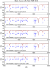 |
Fig. C.2 Same as Fig. C.1, but for the wavelength range λ4400–5500Å. |
| In the text | |
Current usage metrics show cumulative count of Article Views (full-text article views including HTML views, PDF and ePub downloads, according to the available data) and Abstracts Views on Vision4Press platform.
Data correspond to usage on the plateform after 2015. The current usage metrics is available 48-96 hours after online publication and is updated daily on week days.
Initial download of the metrics may take a while.