| Issue |
A&A
Volume 698, June 2025
|
|
|---|---|---|
| Article Number | A300 | |
| Number of page(s) | 17 | |
| Section | Galactic structure, stellar clusters and populations | |
| DOI | https://doi.org/10.1051/0004-6361/202554658 | |
| Published online | 23 June 2025 | |
A hybrid SLAM-Payne framework for atmospheric parameter and abundance determination of early-type stars from LAMOST DR9 low-resolution spectra
Leibniz-Institut für Astrophysik Potsdam (AIP),
An der Sternwarte 16,
14482
Potsdam,
Germany
★ Corresponding author: This email address is being protected from spambots. You need JavaScript enabled to view it.
Received:
20
March
2025
Accepted:
13
May
2025
Abstract
Context. Early-type stars are key drivers of Galactic chemical evolution, enriching the interstellar medium with alpha elements through powerful stellar winds and core-collapse supernovae, fuelled by their short lifetimes and high masses. However, their spectra remain challenging to analyse due to rapid rotation, weak metal lines, and non-local thermodynamic equilibrium (NLTE) effects. While large spectroscopic surveys provide extensive low-resolution data, extracting reliable parameters remains difficult due to methodological limitations for hot stars.
Aims. Our goal is to develop a unified framework that combines data-driven and synthetic spectral approaches to determine atmospheric parameters and abundances for hot stars using low-resolution spectra, thereby addressing limitations in current methodologies while retaining critical spectral information.
Methods. We present a hybrid approach integrating the Stellar LAbel Machine (SLAM) and the Payne frameworks, for low-resolution (R~1800) spectra from LAMOST DR9. Our method preserves full spectral information including Balmer series and metal-line blends, employing neural-network interpolation for efficient parameter estimation (Teff, log g, and v sin i) and abundance determination for O, Mg, Si, and Fe, across 8000 K–20 000 K.
Results. We derive stellar parameters and abundances for 315 822 stars with S/N ⩾ 10 in the r-band. Among these, we identify 3564 blue horizontal branch candidates, over 90% of which align with stellar evolutionary models of horizontal branch stars. Additionally, we detect abundance trends ([α/Fe]–[Fe/H]) that exhibit temperature-dependent systematics and a distinct α-poor stellar population within 0.0 ⩽ [Fe/H] ⩽ 0.5 dex. The radial abundance gradients are negative and consistent with that derived from Cepheids, with a slope of −0.070 ± 0.007 in [Fe/H] in the region 6 ⩽ RGC ⩽ 15 kpc.
Key words: stars: abundances / stars: early-type / Galaxy: abundances / Galaxy: stellar content
© The Authors 2025
 Open Access article, published by EDP Sciences, under the terms of the Creative Commons Attribution License (https://creativecommons.org/licenses/by/4.0), which permits unrestricted use, distribution, and reproduction in any medium, provided the original work is properly cited.
This article is published in open access under the Subscribe to Open model. This email address is being protected from spambots. You need JavaScript enabled to view it. to support open access publication.
1 Introduction
Early-type stars, with effective temperatures exceeding 7500 K, serve as critical astrophysical laboratories for studying stellar evolution and Galactic chemical enrichment. These stars not only dominate the ultraviolet radiation budget of galaxies (Maeder & Conti 1994), drive chemical mixing through intense stellar winds (Puls et al. 2008), and ultimately explode as supernovae that disperse heavy elements into the interstellar medium (Zinnecker & Yorke 2007), but also are tracers of the young stellar populations within the Galaxy (Venn 1995; Carraro et al. 2010). In particular, understanding the detailed atmospheric parameters and chemical compositions of hot stars is essential for unravelling the complex interplay between stellar evolution and Galactic chemical evolution (e.g. Eldridge & Stanway 2022). The radial metallicity gradient inferred from this young population traces the current state of the disc abundance profile (Bragança et al. 2019). Together with the metallicity profiles of older mono-age populations (Lian et al. 2023), these gradients are important observational constraints for models of Galactic chemical evolution (Maiolino & Mannucci 2019).
Despite their importance, large-scale spectroscopic analyses of hot stars remain challenging due to their rapidly rotating atmospheres, weak metal-line features, and complex non-localthermodynamic equilibrium (NLTE) effects. The spectral ‘analysis of hot stars presents unique challenges compared to their cooler counterparts. High rotation rates broaden absorption features (Royer et al. 2007), while elevated temperatures reduce line densities and enhance NLTE effects (Lanz & Hubeny 2007). These factors as well as internal mixing processes and the possible presence of chemical peculiarities, complicate the determination of fundamental parameters (Teff, log g, and v sin i) and chemical abundances from low-resolution spectra. Traditional methods developed for FGK stars often fail to account for the blended Balmer-line profiles and pressure-broadening effects that dominate hot-star spectra (Takahashi & Langer 2021). Consequently, previous studies of hot stars have largely relied on high-resolution spectroscopy (e.g. Dunstall et al. 2015), limiting sample sizes to ~103 stars despite the availability of ~106 spectra in public surveys like the Sloan Digital Sky Survey (SDSS; Almeida et al. 2023) and the Large Sky Area MultiObject Fiber Spectroscopic Telescope (LAMOST; Deng et al. 2012). Although the upgraded spectral resolution of LAMOST’s Medium-Resolution Survey (MRS; R ~ 7500) offers new opportunities for studying the abundances of hot stars, its limited wavelength coverage constrains the precise determination of surface gravity (log g) and chemical abundances.
Recent advancements in data-driven spectral analysis have opened new avenues for tackling these challenges. Methods such as the Payne (Ting et al. 2019) and Stellar LAbel Machine (SLAM; Zhang et al. 2020a) have demonstrated that it is possible to extract detailed stellar labels even from spectra with moderate resolution. Xiang et al. (2022) introduced the HotPayne method, a spectral analysis tool built upon the Payne method but specifically designed for hot stars. Aside from the difference in temperature range, HotPayne masks the Hydrogen lines to resolve the reverse of spectral gradients for the A0 stars. While this approach successfully mitigates the impact of hydrogen lines for the A0 stars, an essential part of the information is lost. On the other hand, the SLAM method, building upon Guo et al. (2021); Sun et al. (2021a), has proven effective in deriving parameters. Notably, Sun et al. (2021b); Sun & Chiappini (2024) leveraged LAMOST’s MRS DR 9 to catalogue over 100 000 late-B- and A-type MS stars, with Teff spanning from 7000 K to 15 000 K. They uncover a bimodal rotation distribution that varies with stellar mass and is influenced by metallicity, suggesting a significant role of chemical composition in the rotational evolution of A-type stars on the main sequence. Recently, the SLAM method has been expanded to include photometric information to better constrain the stellar temperature, and has been applied to a subset of blue horizontal branch (BHB) stars (Ju et al. 2025), selected by the equivalent widths of multiple absorption line profiles (Ju et al. 2024).
Each of these methods has its strengths and limitations; for instance, while SLAM excels in robustness and consistency for temperature determinations, its scalability is limited by slower inference times when handling extensive training sets and high-dimensional label spaces. The Payne framework, on the other hand, enables efficient and flexible abundance determinations across a wide parameter space, but its reliance on the accurate modelling of spectral gradients can lead to reduced reliability in regions where the spectral response is highly nonmonotonic. These shortcomings motivate the development of a unified framework that combines the strengths of data-driven and synthetic spectral approaches. This study addresses these challenges through a synergistic analysis of LAMOST Low-Resolution Survey (LRS; R ~ 1800) DR9 spectra using complementary methodologies. Building upon our previous work with SLAM (Sun et al. 2021a; Sun & Chiappini 2024), we incorporate Payne’s flexible spectral model to enable abundance determinations for four key elements (O, Mg, Si, and Fe) across the 8000 K–19 000 K temperature range. Our approach retains the full spectral information content – including the diagnostically critical Balmer series and the metal-line blends – while maintaining computational efficiency through neural network interpolation. We validated the method against high-resolution benchmarks and quantified systematics arising from differences in spectral modelling techniques. The resulting catalogue of 315 822 stars with r-band S/N ⩾ 10 represents a homogeneous dataset of hot-star parameters and abundances, providing simultaneous determinations of Teff, log g, v sin i, and elemental abundances without excluding broadened features.
The paper is organised as follows: Section 2 describes our source catalogue and pre-selection. Our hybrid SLAM-Payne framework is detailed in Section 3, with a performance validation for precision. Then we present the accuracy test of our measurement in Section 4, via verification against high-resolution data and comparison against low-resolution data. Section 5 presents the stellar parameter catalogue with abundance measurements and identification of distinct stellar populations, including BHB stars and metal-rich outliers. We also discuss the photometric selection and abundance distribution of the sample as well as the abundance gradients across the Milky Way disc. We conclude in Section 6 with a summary of our key findings and implications.
2 Data
Our sample of early-type stars is compiled from the low-resolution (R ~ 1800) spectra in the ninth data release (DR9) of the LAMOST Experiment for Galactic Understanding and Exploration (LEGUE) surveys (Deng et al. 2012; Zhao et al. 2012; Liu et al. 2014). The LAMOST, a 4 m reflective Schmidt telescope, provides low-resolution spectra with a wavelength coverage of 370–910 nm. Its DR9 Version 2.0 spans observations from October 24, 2011, to June 12, 2021, containing 10 809 336 spectra, with 10 495 781 classified as stellar spectra. In addition to source catalogues, the release provides a stellar parameter catalogue for 6 921 466 spectra of A, F, G, and K stars, deriving Teff, log g, [Fe/H], and [α/M] from the LAMOST Stellar Parameter Pipeline (LASP, Luo et al. 2015).
The primary catalogue of early-type stars is constructed using the source catalogue, supplemented with Gaia DR3 and Two Micron All Sky Survey (2MASS; Skrutskie et al. 2006) for photometric determination, and follows Riello et al. (2021)’s guidelines for Gaia astrometric and photometric parameters. We adopt the photo-geometric distance estimates from Bailer-Jones et al. (2021), who derived distances using EDR3 parallaxes (corrected for the zero-point offsets in parallax) within a 3D Galactic model.
We applied two selection criteria to refine the early-type candidates:
Objects with LASP-derived effective temperatures below 7500 K were excluded, consistent with Sun et al. (2021a). The remaining sample included stars above this threshold and those lacking LASP temperature estimates, e.g. early-type stars and M/K-type dwarfs (see Figure 2 in Sun et al. 2021a).
Using the approach proposed in Zari et al. (2021), we utilised the proxy of the absolute magnitude of a star in the Ks band, denoted as
![Mathematical equation: $\[tilde{M}_{K_{s}}]$](/articles/aa/full_html/2025/06/aa54658-25/aa54658-25-eq1.png) . We set a limit for the cool end of the spectral types, requiring that
. We set a limit for the cool end of the spectral types, requiring that ![Mathematical equation: $\[tilde{M}_{K_{s}}]$](/articles/aa/full_html/2025/06/aa54658-25/aa54658-25-eq2.png) , defined as Ks − 5 log10(r) + 5, be smaller than 2.5 mag. No additional selections based on colours (e.g. J − Ks or G − Ks) were applied. This magnitude cut roughly corresponds to the absolute magnitude of an F6V star with Teff = 6350 K (Pecaut & Mamajek 2013).
, defined as Ks − 5 log10(r) + 5, be smaller than 2.5 mag. No additional selections based on colours (e.g. J − Ks or G − Ks) were applied. This magnitude cut roughly corresponds to the absolute magnitude of an F6V star with Teff = 6350 K (Pecaut & Mamajek 2013).
Either of the criteria removes approximately 60% of the candidates from the source catalogue. When combined, these criteria leave 1 833 153 spectra of 1 405 917 stars.
3 Method
3.1 Pipeline
One of the major difficulties in determining spectral labels from early-type stars’ spectra originates from the non-monotonic trend of hydrogen line strength. The equivalent widths of the Balmer lines reach a maximum around 9000 K due to the relatively high excitation energy of the Balmer series (10.2 eV) (Gray & Corbally 2009). In late-type stars, hydrogen lines are weak but steadily stronger with increasing effective temperature until reaching a maximum in early A-type stars. At higher temperatures (B- and O-type stars), the hydrogen lines again become weaker. As the dominant feature for effective temperature diagnostics, this near-zero gradient in hydrogen line strength creates an inflection point around Teff ~ 9000 K, making temperature estimates sensitive to initial values and potentially creating artefacts of temperature void around the peak.
This effect has been observed in several spectral analysis methods, including the modules described in Blomme et al. (2022), where different analysis nodes for hot-star spectra in the Gaia-ESO survey were investigated. While χ2 minimisation methods are generally robust, machine-learning approaches may be affected by this issue due to the sign change in spectral gradients around A0-type stars. To address this, Xiang et al. (2022) devised a spectral masking technique to exclude hydrogen lines during label determination for early A-type and late B-type stars. However, masking hydrogen lines reduces spectral information content, leading to lower precision in determining Teff and log g. They combined results from analyses with and without masked hydrogen lines to produce final estimates, which resolved the spurious absence of A0-type stars and unexpected Kiel diagram patterns around 10 000 K (Xiang et al. 2022), though at the cost of information loss for stars near A0-type.
The SLAM method solves this problem through several advantages inherent to its data-driven approach using support vector regression (SVR). Unlike gradient-based methods, SVR employs dual optimisation with Lagrange multipliers through quadratic programming, avoiding direct gradient calculations of loss functions. The Karush-Kuhn-Tucker conditions in SVR’s dual form provide stationary point solutions analogous to gradient-based optima but without gradient descent. Additionally, SLAM automatically determines hyperparameters (penalty level and tube radius) through the training set itself, enabling pixel-wise adaptive model complexity that particularly benefits hydrogen line analysis around A0 stars. This capability was demonstrated in our previous work (Sun et al. 2021a), where SLAM analysis of LAMOST MRS showed no anomalous temperature gaps (see their Fig. 9). While log g accuracy from MRS remained limited due to the restricted wavelength coverage (5000–5300 Å and 6350–6800 Å), we anticipate improvement with the broader coverage of LRS.
We complement SLAM with an Artificial Neural Network model based on the Payne algorithm to estimate additional abundances. This hybrid approach addresses SLAM’s computational limitations as Support Vector Machine complexity scales between 𝒪(nfeatures × nsamples2) and 𝒪(nfeatures × nsamples3) (Chang & Lin 2021), making comprehensive label coverage impractical. Our implementation uses SLAM for four fundamental parameters (Teff, log g, [Fe/H], and v sin i), while employing the Payne model for other abundances using an extensive training library with complete label space coverage.
Our pipeline proceeds as follows: first, we obtained bestfit labels from SLAM. These parameters then fixed Teff, log g, [Fe/H], and v sin i in a subsequent Payne module run to determine remaining abundances. We reported associated uncertainties using standard propagation methods.
For spectral preprocessing, we normalised spectra and corrected for radial velocity using laspec1 (Zhang et al. 2021). The normalisation iteratively fitted a spline function three times, rejecting pixels deviating >3σ from median values in 100 Å windows. We adopted line-of-sight velocity corrections from LAMOST pipeline-reduced spectral headers.
Section 3.2 describes our template grid and synthetic spectra. Training procedures for SLAM and Payne modules appear in Sections 3.3 and 3.4, respectively, followed by performance evaluation in Section 3.5.
Range and sampling method of the stellar labels for training.
3.2 Grid synthesis
We constructed a grid comprising 𝒩 sets of stellar labels in 11D parameter space (Teff, log g, [Fe/H], microturbulence vmic, v sin i, [C/Fe], [O/Fe], [S/Fe], [Mg/Fe], [Ca/Fe], and [Si/Fe]). The label selection follows recommendations from Xiang et al. (2022), who used Cramér–Rao bounds to assess theoretical precision limits for hot-star label determination from LAMOST LRS. For Teff and log g, we sample MIST isochrones (Paxton et al. 2011; Choi et al. 2016) using equivalent evolutionary phase (EEP) via isochrones (Morton 2015). To ensure smooth label distributions, we perturbed these values with normal distributions (σ = 250 K for Teff, σ = 0.25 dex for log g), then restricted to Teff ∈ [7000, 20 000] K and log g ∈ [0.0, 5.0] dex.
We sampled [Fe/H] uniformly between −2.5 and 1.0 dex, while other abundances follow uniform distributions scaled relative to [Fe/H] using the solar abundance scale of Asplund et al. (2009). Microturbulence vmic ranges uniformly from 0 to 10 km s−1. For v sin i, we adopted the log-normal distribution from Sun et al. (2021a) with peak at 90 km s−1 and tail extending to ~400 km s−1. Table 1 summarises the training grid.
We generated synthetic spectra using SYNTHE with Kurucz LTE atmospheric models from ATLAS12 (Kurucz 2005). Broadening by microturbulence and rotation was applied via vidmapy2 at R = 100 000. To match LAMOST-LRS instrumental characteristics, we applied wavelength-dependent Gaussian line spread functions (LSFs) determined by comparing high-S/N (> 100) FGK star observations to unbroadened synthetics. The wavelength-varying resolution was approximated by fifth-order polynomials across the blue (3700–5800 Å) and red (5700–9100 Å) arms. We added Gaussian noise equivalent to S/N = 1000 per pixel.
While ATLAS12 assumes LTE, Przybilla et al. (2011) demonstrated that LTE models remain adequate for main-sequence stars below 22 000 K, justifying our 20 000 K upper limit. Synthetic spectra are computed in absolute flux units, including continuum and line contributions. After applying instrumental effects, we resampled these spectra to LRS coverage (1 Å per pixel) and normalised them using the iterative spline-fitting procedure described in Section 3.1, which operates on the total flux and reject >3σ outliers in 100 Å windows. Observed raw spectra underwent the same resampling and normalisation process to ensure consistency. We adopted the line list from the Superfast line profile variability (LPV) project3, which combines OBA star line lists from Reader et al. (1980), Striganov & Sventitskii (2013), and the NIST database4.
3.3 SLAM module
The SLAM module follows the methodology outlined in Sun et al. (2021a), employing two specialised models: (1) a high-resolution converter mapping synthetic spectra to fundamental parameters (Teff, log g, [Fe/H]) within predefined ranges, and (2) a mock spectrum generator producing LRS-like spectra through rotational and instrumental broadening. We mask known diffuse interstellar bands (Hobbs et al. 2008) and exclude the Hα region (6552.0–6572.0 Å) to avoid emission line contamination.
Hyperparameter optimisation uses ϵ = 0.05 (tube radius), C ∈ {0.1, 1, 10} (penalty), and γ ∈ {0.1, 1, 10} (RBF kernel width), selected via five-fold cross-validation. Computational constraints limit our training sample to 5000 stars, balancing model performance with resource requirements.
3.4 Payne module
We implement the Payne algorithm (Ting et al. 2019) to predict flux variations across the 11D parameter space listed in Table 1. Our architecture in PyTorch features two hidden layers (40 neurons each) and an output layer with a size of 5400. These layers are connected with sigmoid activations for smooth interpolation between stellar parameters. The spectral library splits into training (70%) and validation (30%) sets, with mean squared error evaluated every 5000 epochs during optimisation. We utilise the ADAM optimiser (Kingma & Ba 2014) with a learning rate of 0.001, monitoring validation loss to prevent overfitting.
3.5 Performance
We validate the spectroscopic model’s performance on synthetic data prior to application to observations. A test set of 5000 spectra – following the training label distribution but spanning S/R = 50–1000 – is generated independently of the training process. The full pipeline (SLAM + Payne modules, Sect. 3.1) is applied to evaluate three key metrics: (1) pixel-level spectral reconstruction (Appendix A), (2) label recovery accuracy across S/N regimes, and (3) consistency between repeated observations of the same target.
Figure 1 shows the SLAM module’s performance in recovering Teff and log g across the Kiel diagram. Results are binned by ΔTeff = 1000 K and Δ log g = 0.5 dex (dashed grey lines). Coloured markers denote standard deviations for S/N = 30 (top), 50, 100, and 250 (bottom) within each populated bin. Two trends emerge: (1) precision improves systematically with S/N, particularly below S/N = 100, and (2) Teff accuracy degrades logarithmically with increasing temperature, from σTeff ≈ 50 K at 7000 K to σTeff ≈ 300 K at 17 000 K. While log g precision remains relatively constant (σlog g ≈ 0.1 dex) across most of the parameter space, tentative degradation occurs for Teff > 16 000 K giants (log g < 3.5 dex), likely due to reduced line density in evolved stars.
In Fig. 2, we present the scatter (solid) and bias (dashed) of different labels as a function of S/N. The parameters Teff, log g, [Fe/H], and v sin i are estimated via the SLAM module, while the remaining labels are derived from the Payne module.
We categorised the test sample into three temperature ranges: 7000 K < Teff < 9000 K (blue), 9000 K < Teff < 13 000 K (green), and 13 000 K < Teff < 17 000 K (orange). A representative example at S/N = 100.0 (without Teff selection) is shown, with the bias (μ) and scatter (σ) for each label marked in the upper-right corner of the corresponding panel. For nearly all labels, the most pronounced trend across the three subpopulations is the performance improvement (i.e. decreasing bias and scatter) with increasing S/N. This reflects the expected reduction in noise contamination at higher S/Ns. However, [C/Fe], [S/Fe], and [Ca/Fe] exhibit a weaker dependence of σ on S/N, with persistently large scatter (σ > 0.35). This indicates that, given the resolution and wavelength coverage of LAMOST LRS, the current model cannot reliably recover these abundances.
By comparing the behaviour of subsamples with different temperatures, we find that the remaining labels can be largely classified into two groups based on the degree of temperature dependency. For [O/Fe], [Mg/Fe], and [Si/Fe], different subsamples show very similar profiles in their scatter and bias, with average scatters at S/N = 100 of 0.22, 0.14, and 0.17, respectively.
In contrast, the results for the other labels vary significantly among different temperatures. As stars become hotter, most spectral features available for measuring the labels weaken, which largely explains the trend observed in Fig. 2. Hotter stars generally exhibit larger scatter in Teff compared to cooler stars. Microturbulence (not included in Fig. 2) displays similar behaviour to Teff and v sin i, with a typical uncertainty of μ = −0.07 km s−1 and σ = 0.58 km s−1 at S/N = 100. The variation of log g with temperature is not significant, as shown in Fig. 1. The dependency on Teff is particularly important for [Fe/H], where the absolute value of bias significantly increases with higher temperatures. This again illustrates the difficulty of inferring abundance for hotter stars using low-resolution spectra and hints at a possible missing population of hot, metal-poor stars. However, for other labels we do not observe such a strong dependence on bias of [X/Fe], which may be due to the relative ratios between the spectral lines of a given abundance and those of iron.
While these tests demonstrate the accuracy of the model reconstruction and establish the minimum uncertainty for the recovered parameters, larger uncertainties could be expected for observed data. This is due to various factors, such as the physical complexity of model atmospheres, synthetic spectra, and characteristics of the observed data (including data reduction effects), which contribute to the overall uncertainties. We then use targets with repeated observations and take the scatter of the labels inferred from these observations as the precision of the Payne model.
Fig. 3 presents the scatter of labels between repeated observations. This is based on 36 563 spectra of 2034 stars, with a median observation number of nine. The S/Nr is defined as the average value of the S/N in the r band, and the scatter is calculated as the standard deviation of the labels among repeat observations for a given star, weighted by their S/Ns. The median value of the scatter in bins of size 50 in S/N is shown in orange, demonstrating a photon noise-dominated phase for low S/N. We adopt the median value of the scatter as the precision of our sample, which is 163 K for Teff, 0.12 dex for log g, 0.10 dex for [Fe/H], 18.8 km s−1 for v sin i, 0.5 km s−1 for vmic (not included in Fig. 3), and approximately 0.2 dex for [X/Fe]. This is roughly consistent with the estimate in Fig. 2 to within a factor of 2, despite differences in the samples used in the two tests.
Given the large uncertainties of [C/Fe], [S/Fe], and [Ca/Fe], we excluded C, S, and Ca from subsequent analysis. Therefore, aside from iron abundance, we present the results for the three α-elements ([O/Fe], [Mg/Fe], and [Si/Fe]) for the sample.
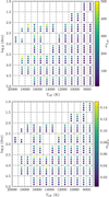 |
Fig. 1 Recovery precision for Teff (top) and log g (bottom) from the SLAM module across the Kiel diagram. Test spectra are binned by ΔTeff = 1000 K and Δ log g = 0.5 dex (delineated by dashed grey lines). For each bin with a significant number of spectra, the four ‘traffic light’ bullets show the standard deviation of the label for S/Ns of (top to bottom) 30, 50, 100, and 250. Empty bins contain insufficient data for robust statistics. |
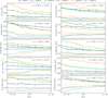 |
Fig. 2 Label recovery precision versus signal-to-noise ratio (S/N per Å) for the spectroscopic pipeline. Solid and dashed lines represent scatter (σ) and bias (μ), respectively, calculated within S/N bins. Coloured bands indicate three temperature regimes: 7000 K < Teff < 9000 K (blue), 9000 K < Teff < 13 000 K (green), and 13 000 K < Teff < 17 000 K (orange). Insets show σ and μ values at S/N = 100 in the units applicable to the respective labels for the full sample. |
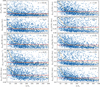 |
Fig. 3 Scatter of labels between repeated observations. The S/Nr is defined as the average value of the S/N in the r band of the observations, and the scatter Δrepl is the standard deviation of the labels in the units applicable to the respective labels, weighted by their S/N. Dashed orange lines represent the median value of the scatter in each S/N bin. Horizontal red lines indicate the median value of Δrepl from the entire sample with repeated observations, which are also marked in the top-right corner. |
4 Method validation
In this section, we present verification and comparison results with literature studies. We separate these into two parts: verification against high-resolution data (Sect. 4.1) and comparison against low-resolution data (Sect. 4.2). We define high resolution as spectral resolutions exceeding R = 10 000.
4.1 Verification against high-resolution data
Given the brightness limitations of the LAMOST LRS, relatively few reference stars have well-established parameters and abundances derived from high-resolution NLTE spectroscopy. We therefore combined reference stars with published NLTE/LTE analyses and synthetic spectra generated from high-resolution observations.
Our verification sample incorporates benchmark stars from Przybilla et al. (2006), Takeda et al. (2008), and Gebruers et al. (2021). Using FEROS echelle spectra (R ~ 48 000) from the MPG/ESO 2.2-metre telescope, Przybilla et al. (2006) developed a hybrid NLTE spectrum synthesis technique to analyse four BA-type supergiants, deriving abundances for He, C, N, O, Mg, S, Ti, and Fe. Takeda et al. (2008) obtained R ~ 45 000 spectra with the Bohyunsan Observatory Echelle Spectrograph on the 1.8 m reflector, measuring abundances of seven elements in 46 bright A-type stars while considering NLTE effects exclusively for the O I triplet at 7771–7775 Å. Gebruers et al. (2021) analysed R ~ 85 000 HERMES spectra from the 1.2 m Mercator telescope for 111 pulsating stars, determining atmospheric parameters via the Grid Search in Stellar Parameters method (Tkachenko 2015) under LTE assumptions. Fig. 4 displays the benchmark stars’ temperature-gravity distribution (top) and chemical abundances (bottom). The sample spans effective temperatures of 8000–19 000 K and iron abundances from ~−1.0 dex to ~+0.5 dex, including three giants (log g < 3.5). We identify tentative correlations between [O/Fe] and [Fe/H], as well as between [Si/Fe] and [Fe/H], though larger samples are needed to confirm these trends.
The verification results appear in Fig. 5, showing differences between our derived labels and literature values as functions of effective temperature. For stars from Przybilla et al. (2006) and Takeda et al. (2008) that are too bright for LAMOST-LRS, we retrieve archival XSHOOTER/UVES spectra degraded to LAMOST resolution (open squares). Literature [X/Fe] values were calculated from published [X/H] and [Fe/H] measurements.
Our results show good consistency for Teff, log g, and v sin i without systematic trends with temperature. One supergiant (log g = 1.20, not shown in Fig. 5) exhibits significant offsets: Δ log g = −0.6 dex and Δ v sin i = +150 km s−1, likely from NLTE effects influencing both gravity and rotation measurements.
Iron abundances generally match literature values with temperature-independent scatter (σ[Fe/H] ~ 0.2 dex). While deviations increase slightly for Teff > 15 000 K, this coincides with larger literature uncertainties. Hot metal-poor stars ([Fe/H] < −0.5 dex, Teff > 15 000 K) may show underestimated metallicities, consistent with the negative bias for hot stars in Fig. 2. Light elements demonstrate varying performance: [Mg/Fe] and [Si/Fe] show minimal temperature dependence with σ ~ 0.3 dex, though the hottest stars exhibit slight underestimates. This could arise from literature [Fe/H] overestimates affecting abundance ratios. Oxygen abundances display larger scatter (σ[O/Fe] ~ −0.4 dex) without clear temperature trends.
Our verification demonstrates good agreement with high-resolution studies across Teff (7500–20 000 K) for fundamental parameters and key abundances. Scatter remains within 0.2 dex for [Fe/H], 0.3 dex for [Mg/Fe] and [Si/Fe], and −0.4 dex for [O/Fe], comparable to literature uncertainties. Increased dispersion at the hot end reflects intrinsic measurement challenges and potential systematic differences between analysis methods.
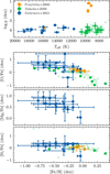 |
Fig. 4 Kiel diagram (top panel) and abundance patterns (bottom panel) for benchmark stars. Symbols denote different literature sources: Przybilla et al. (2006, orange), Takeda et al. (2008, green), and Gebruers et al. (2021, blue). Faded markers indicate stars lacking available spectra for direct verification. |
4.2 Comparison against low-resolution data
While high-resolution spectroscopy provides precise benchmarks, comparison with LRSs remains essential for validating pipeline performance across large samples. The statistical power of LRS datasets enables the detection of population-level trends obscured in smaller high-resolution samples, though reduced spectral resolution requires careful systematic error assessment.
We compare our results with two major studies: Xiang et al. (2022) using LAMOST LRS (R ~ 1800) with the HotPayne method, and Sun et al. (2021a) analysing LAMOST MRS (R ~ 7500) spectra covering 4950–5350 Å and 6300–6800 Å. For robust comparison, we restrict the LRS-based sample to stars with S/Nr > 100. The cross-matched sample with Xiang et al. (2022) consists of 65 590 stars, while the overlap with the MRS-based analysis includes 8078 stars, spanning 7000–14 500 K with median S/Ng ~ 40. Additionally, 10713 stars are common to both external catalogues.
Fig. 6 compares four key parameters across studies. Effective temperatures (Panel a) show good agreement (σ = 442 K) between this work and Xiang et al. (2022), across the entire temperature range. The MRS comparison reveals a ~5% coolward bias below 12 000 K, potentially from differences in wavelength coverage between LRS and MRS, i.e. MRS only covers the H α line. Enhanced scatter around A0-type stars (9000–11 000 K) suggests challenges in modelling Balmer line morphology transitions in LRS data (see Fig. 7). This may also explain the difference of scatter when we cross-match the results to Sun et al. (2021a), where the top-left panel shows a tighter correlation compared to the bottom-right one.
As for surface gravity comparisons (Panel b), we focus on Xiang et al. (2022) since MRS spectra provide limited log g constraints due to their narrow wavelength coverage (Zhang et al. 2020b). Our log g measurements show a systematic offset of 0.11 dex relative to Xiang et al. (2022), predominantly driven by stars in the 9000–11 000 K range. The white contours in Fig. 6 explicitly demonstrate how this temperature-dependent bias distorts the correlation. We attribute this discrepancy to differences in gravity-sensitive feature selection between pipelines, particularly for A-type stars, where Balmer line profiles dominate LRS spectra.
Metallicity comparisons (Panel c) reveal good overall agreement with Xiang et al. (2022) (σ[Fe/H] ~ 0.21 dex). We identify a −0.14 dex systematic offset for stars near solar metallicity ([Fe/H] ≈ 0), which diminishes at both metal-rich ([Fe/H] > +0.3) and metal-poor ([Fe/H] < −0.5) extremes. This pattern persists across the 9000–11 000 K subsample (white contours), suggesting temperature-independent calibration differences rather than physical abundance variations. The bias when compared against Sun et al. (2021a) could be attributed to the difference between [Fe/H] and [M/H].
The last panel presents the comparison for v sin i. This work and Xiang et al. (2022), both based on LAMOST-LRS, are consistent with each other and largely follow the same profile when compared with Sun et al. (2021a). In particular, rotational velocities derived by Sun et al. (2021a) are larger than those derived in this work for v sin i ⩽ 100 km s−1 and are in good agreement for larger values. This behaviour is expected due to the medium-resolution data used in Sun et al. (2021a).
To investigate label differences across stellar spectral types, Fig. 7 displays label variations as a function of effective temperature. The subplots, from top to bottom, show the differences Δl = lXiang − l for the four atmospheric parameters Teff, log g, [Fe/H], and v sin i derived from the SLAM module. Similar to Fig. 6, Teff values show generally good agreement, though the difference distribution becomes asymmetric about Δl = 0 (dashed line) for stars between 9500 K (log Teff ~ 3.95) and 11 000 K (log Teff ~ 4.05). A comparable asymmetry appears in the log g panel (second row). As noted previously, this likely stems from the HotPayne approach employed by Xiang et al. (2022), which masks Balmer line regions when analyzing A0-type stars – a simplification that degrades label recovery performance, particularly for Teff and log g.
The [Fe/H] panel (third row) reveals a systematic offset of −0.13 dex, most pronounced below Teff < 10 000 K. This metallicity bias gradually diminishes with increasing temperature, culminating in a steep transition near the grid boundary at Teff ~ 19 000 K (log Teff ~ 4.25). The v sin i panel (bottom row) features a temperature-independent horizontal line at −5 km s−1, reflecting differing lower limits in rotational velocity between studies. Our analysis adopts a 5 km s−1 minimum for projected rotational velocity, compared to the 0 km s−1 threshold used by Xiang et al. (2022). This discrepancy produces an artificial offset population corresponding to slow rotators present in both samples.
We further analyse the v sin i distribution by comparing our results with two other studies, focusing on low rotational velocities. Accurate determination of projected rotational velocity from low-resolution spectra (LAMOST-LRS) is challenging at small v sin i values, as rotational broadening blends with instrumental broadening. Fig. 8 shows the v sin i distributions and complementary cumulative distribution functions. Results from the two LAMOST-LRS studies agree well with LAMOST-MRS measurements for v sin i ⩾ 200 km s−1. However, we note an anomalously high fraction of slow rotators (v sin i ⩽ 20 km s−1) in Xiang et al. (2022), despite these velocities being below typical detection limits. Discrepancies emerge at lower velocities: For v sin i = 100–200 km s−1, Xiang et al. (2022) shows a 10–20% deficit compared to Sun et al. (2021a), while our results differ by < 5% from the latter. This trend appears more clearly in the cumulative distribution (bottom panel), where the distributions begin to diverge below 100–120 km s−1. Previous spectral resolution studies (Sun et al. 2019, 2021b) estimate a 120 km s−1 detection limit for LAMOST-LRS (dashed grey line in Fig. 8), consistent with the velocity range where significant discrepancies occur. This suggests improved v sin i accuracy in our work for v sin i > 120 km s−1, though results below this threshold should be interpreted cautiously.
These comparisons reveal how spectral resolution and methodology affect parameter determination. While high-resolution data provide precision benchmarks, the consistency between low-resolution studies demonstrates our pipeline’s robustness for large samples. Systematic biases in log g and [Fe/H] for A0 stars, however, highlight limitations in both the HotPayne method and data processing approaches when critical spectral features are masked.
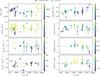 |
Fig. 5 Label differences Δl = llit − l between literature results from high-resolution spectroscopy and this work, plotted against Teff. Coloured symbols denote benchmark stars with high-resolution data, where colour intensity corresponds to label values. Circles indicate stars with LAMOST LRS spectra, while empty squares represent spectra mimicked from high-resolution observations. Error bars and upper limits reflect uncertainties from Przybilla et al. (2006), Takeda et al. (2008), and Gebruers et al. (2021). |
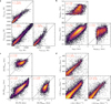 |
Fig. 6 Parameter comparisons with Xiang et al. (2022, LRS) and Sun et al. (2021a, MRS). Colour density scales with log(N). Panels b–c overlay contours (white) for 9000–11 000 K stars. Dashed lines show 1:1 relations, with red text indicating mean offsets (μ) and standard deviations (σ). |
5 Results
In this study, we employed the SLAM method in conjunction with the Payne model to produce a catalogue of stellar properties for early-type stars derived from LAMOST LRS DR9. This section outlines our sample filtering criteria for the final catalogue and provides examples of how our catalogue can investigate the early-type stellar population within the survey’s footprint, including the BHB stars, abundance distribution, and abundance gradient.
5.1 Sample filtering
We implement a selection criterion based on the S/N in the r band, excluding spectra with S/N lower than 10. As illustrated in Fig. A.2, the spectral information for early-type stars is limited, particularly for those with higher effective temperatures. To ensure the reliability of our results across different temperature ranges, we recommend a more conservative S/N threshold of 50, especially for users interested in abundance determinations. Additionally, we apply several cuts based on the Hess diagram of the remaining candidates.First, we discard stars with Teff ⩽ 7100 K, as those near the lower boundary are likely to be cooler stars with Teff ⩽ 7000 K. This exclusion removes more than half of the candidates from the sample. Similarly, we impose a cut at 19 000 K to eliminate stars with potentially higher temperatures. These temperature cutoffs are informed by comparisons with existing studies, specifically Luo et al. (2015); Sun et al. (2021a); Xiang et al. (2022).
We present the Kiel diagram of our sample in Fig. 9, overlaid with MIST evolutionary tracks for stars ranging from 1.7 to 7.0 M⊙. An abnormal feature is evident in the top-left corner of the Kiel diagram, extending from the hot dwarf region towards cooler giants. By comparing this with catalogues extending to higher temperatures, we confirm that these features are artefacts arising from hotter stars beyond the limitations in the temperature grid (Teff = 20 000 K). Consequently, we exclude all candidate stars above the dashed line. Ultimately, the final sample consists of 315 822 stars with S/N ⩾ 10 and 195 004 stars with S/N ⩾ 50. In contrast to the results presented in Xiang et al. (2022) (see their Fig. 13), we do not observe a vertical stripe of stars extending to low log g values. As noted by Xiang et al. (2022), this feature is an artefact caused by a large number of chemically peculiar stars, whose log g values may have been significantly underestimated due to the masking of hydrogen lines during label determination for early A-type and late B-type stars.
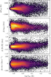 |
Fig. 7 Difference Δl = lXiang − l as a function of Teff from the SLAM module. Subplots from top to bottom show results for Teff, log g, [Fe/H], and v sin i, respectively. |
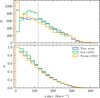 |
Fig. 8 Distribution (N, top) and complementary cumulative distribution functions (ϕ, bottom) of v sin i for cross-matched samples in this work (blue), Sun et al. (2021a) (green), and Xiang et al. (2022) (orange). The dashed grey line at v sin i = 120 km s−1 marks the estimated lower threshold for a reliable v sin i determination at the LAMOST-LRS resolution. |
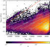 |
Fig. 9 Distribution of candidate stars with r-band S/N > 10 in the Kiel diagram. Stellar density is colour-coded on a logarithmic scale. Temperature cuts at 7100 K and 19 000 K are applied. Stars above the dashed red line represent artefacts from intrinsically hotter stars (Teff ⩾ 20 000 K) and are excluded from further analysis. Grey curves show evolutionary tracks for stars with masses of 1.7, 2.0, 2.5, 3.0, 4.0, 5.0, and 7.0 M⊙ from MIST (Paxton et al. 2011; Choi et al. 2016) models. |
5.2 Photometric selection
The preselection (Sect. 2) and data cleaning (Sect. 5.1) procedures for our sample are primarily driven by spectroscopic criteria. While a selection based on ![Mathematical equation: $\[tilde{M}_{K_{s}}]$](/articles/aa/full_html/2025/06/aa54658-25/aa54658-25-eq3.png) is implemented to eliminate contamination from cooler stars, this approach essentially functions as a magnitude-cutting method that does not utilise colour information, which could enhance sample purity. Therefore, the remaining stars can be used to verify the effectiveness of the photometric selection criteria. Zari et al. (2021) combined Gaia EDR3 astrometry and photometry with 2MASS photometry to create an all-sky sample of luminous OBA-type stars. They employed two sets of selection rules based on the colour-colour diagram and colour-magnitude diagram, defined by the following equations:
is implemented to eliminate contamination from cooler stars, this approach essentially functions as a magnitude-cutting method that does not utilise colour information, which could enhance sample purity. Therefore, the remaining stars can be used to verify the effectiveness of the photometric selection criteria. Zari et al. (2021) combined Gaia EDR3 astrometry and photometry with 2MASS photometry to create an all-sky sample of luminous OBA-type stars. They employed two sets of selection rules based on the colour-colour diagram and colour-magnitude diagram, defined by the following equations:
![Mathematical equation: $\[\begin{aligned}& J-H<0.15\left(G-K_S\right)+0.05, \\& J-H>0.15\left(G-K_S\right)-0.15,\end{aligned}\]$](/articles/aa/full_html/2025/06/aa54658-25/aa54658-25-eq4.png) (1)
(1)
and
![Mathematical equation: $\[G>2\left(G-K_S\right)+3.\]$](/articles/aa/full_html/2025/06/aa54658-25/aa54658-25-eq5.png) (2)
(2)
The first set of criteria selects O- and B-type stars along a sequence in the G − Ks versus J − H colour–colour diagram, accounting for interstellar reddening, which effectively separates these stars from redder turn-off stars and giants. The second set further distinguishes cool giants from OBA stars.
In Fig. 10, we present the distribution of the sample with S/N ⩾ 50 in the J − H versus G − Ks colour–colour diagram (left) and the G versus G − Ks colour-magnitude diagram (right). The photometric selection criteria for OBA stars, as defined by Zari et al. (2021), are indicated by dashed red lines and the shaded grey area. Stellar density is represented on a logarithmic scale, with black contours showing the distribution of the entire sample at kernel density levels of 25%, 50%, and 75%.
Over 95% of our sample falls within the region defined for OBA stars by Zari et al. (2021). However, some outliers may be contaminants from redder turn-off stars and giants. For instance, Zari et al. (2021) attributed the outliers above the dashed red line in the right panel to residual giants. Our estimated stellar parameters for these candidates are primarily clustered near the lower limit of the temperature grid, indicating that they are indeed contaminants.
Apart than this, we note that in the left panel, stars exhibit a broader spread in G − Ks, while the majority are distributed along a shaded region. Although we cannot definitively rule out residual contamination in our sample, these outliers are likely intrinsic hot stars, as their distributions in the Kiel diagram and Teff versus [Fe/H] space show no anomalous clustering. A similar pattern is evident in Fig. 1 of Zhang et al. (2020b) for the LAMOST OB stars from Liu et al. (2019), whose sample was selected based on distributions in spectral line indices (Hγ, Ca II K, He I, and Fe). This highlights potential systematic differences between spectroscopic and photometric selection methods, as discussed in Zari et al. (2021) regarding sample completeness. For example, approximately 9% of the stars in the Liu et al. (2019) catalogue do not satisfy their photometric selection criteria, indicating that approximately 5% to 10% of hot star candidates may be missed.
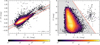 |
Fig. 10 J − H vs G − Ks colour-–colour diagram (left) and G vs G − Ks colour-magnitude diagram (right) for the sample with S/N ⩾ 50. Stellar density is colour-coded on a logarithmic scale. Density contours derived from kernel density estimates are white for the entire sample. Dashed red lines and shaded grey areas delineate the selection criteria for OBA stars as outlined by Zari et al. (2021). |
5.3 Blue horizontal branch stars
Blue horizontal branch stars are old, metal-poor Population II stars with masses less than 1.0 M⊙, typically found in the Galactic halo (Kinman et al. 1994). They are core helium-burning stars located on the blue side of RR Lyrae variables in the Hertzsprung-Russell diagram, characterised by strong hydrogen lines and weak or no molecular bands in their spectra. Their nearly constant absolute magnitude within a restricted colour range makes them useful as distance tracers in studying the Milky Way’s structure and kinematics (e.g. Pier 1984).
In this work, we identify BHB candidates using Galactic latitude (|b|) and iron abundance criteria ([Fe/H]). Fig. 11 reveals that the metallicity distribution of stars with S/Nr ⩾ 50 contains a low-metallicity tail extending from [Fe/H] ~ −1.0 dex. Most metal-poor stars in this tail display significantly smaller projected rotational velocities compared to the main population, approaching the detection limits imposed by the spectral resolution (see Sect. 4.2). These metal-poor stars are preferentially located at greater heights above the Galactic plane, consistent with expectations for BHB stars and blue stragglers. Another subpopulation shows moderate v sin i and high metallicity ([Fe/H] > 0.5 dex), likely corresponding to chemically peculiar stars.
Fig. 12 shows the distribution of BHB candidates in the Teff − log g plane, colour-coded by their projected rotational velocities. Our sample selects stars with Galactic latitude |b| > 15°, metallicity [Fe/H] < −1.4 dex, and spectral signal-to-noise ratio S/Nr ≥ 50, yielding 3564 candidates. Two distinct populations emerge: over 90% of candidates have log g < 3.5 with Teff reaching ~11 000 K, while the remaining 10% reside closer to the main sequence.
We overlay PARSEC isochrones (Bressan et al. 2012) for core-helium-burning horizontal branch stars with metallicities [Fe/H] = −2.5 dex (solid) and −2.0 dex (dashed), computed for ages log(t/yr) = 8.6, 8.8, and 9.0. The isochrones show excellent agreement with stellar parameters for candidates having log g < 3.5 dex, confirming their identification as genuine BHB stars.
The higher surface gravity population (log g ≥ 3.5 dex) likely consists of blue straggler stars (BSS). Notably, BSSs exhibit systematically higher rotational velocities than BHB stars near the horizontal branch. This aligns with expectations that BSS rotation slows through angular momentum loss mechanisms like magnetic braking and disc locking (Leonard & Livio 1995; Leiner et al. 2018). While BHB stars rotate more slowly than young disc stars due to their advanced age, our results suggest they may rotate slower than BSS at comparable metallicities. This is consistent with the scale-width-shape method used in Clewley et al. (2002) and Xue et al. (2008) to differentiate BSS from BHB stars, based on the shapes of the Balmer lines. A small population of horizontal branch stars (~10) exhibit anomalously high rotation (v sin i > 150 km s−1). These outliers likely represent high-luminosity BSS contaminating the horizontal branch region, possibly originating from evolved dwarf stars.
In Fig. 12, we also show the BHB candidates selected from Xiang et al. (2022) as grey points, following the same selection criteria as those applied in this work (with the sole difference being our use of S/N in the g band rather than the r band). We find good agreement in the stellar labels for stars with Teff ~ 8000 K and log g ~ 3.25 dex. However, the labels from Xiang et al. (2022) exhibit significantly higher log g values for BHB stars hotter than this temperature. This discrepancy, as discussed in Sect. 4.2, may arise from the HotPayne method employed in their work, which can lose spectroscopic information near Balmer lines for A-type stars. Further exploration of the completeness of the BHB sample and its usage as distance indicators will be studied in a forthcoming paper (Sun et al., in prep.).
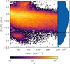 |
Fig. 11 Distribution of stars with S/Nr ⩾ 50 in [Fe/H] and v sin i space. The right subplot displays the logarithmic histogram distribution of [Fe/H], with a horizontal dashed line indicating the metallicity threshold ([Fe/H] = −1.4 dex) for the BHB candidate selection. |
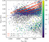 |
Fig. 12 3564 BHB candidates in the Kiel diagram, colour-coded by projected rotational velocities. Grey dots show BHB candidates selected by Xiang et al. (2022) using similar selection criteria. Red lines display PARSEC (Bressan et al. 2012) isochrones for horizontal branch stars with metallicities [Fe/H] = −2.5 dex (solid) and −2.0 dex (dashed), corresponding to ages log(t/yr = 8.6, 8.8, and 9.0 (left to right, respectively). |
5.4 Abundance distribution
Fig. 13 shows the stellar density distributions in abundance space for the sample with S/Nr > 100. We separate the sample into two temperature ranges: cooler than 10 000 K and hotter than 10 000 K. This division reflects the intrinsically different abundance patterns observed between these groups. The verification sample from Sect. 4.1 is shown as coloured circles with error bars, matching the colour scheme of Fig. 4.
The abundance trends align with literature results, particularly for stars cooler than 10 000 K (left panel). However, the [Mg/Fe] and [O/Fe] abundances for hotter benchmark stars lie near the upper envelope of the derived pattern, with some literature values corresponding to the upper limits of chemical abundance measurements. Perfect agreement is not expected due to differences in selection functions between our sample and the literature samples.
We overplot the α elements abundances versus [Fe/H] for a sample of 180 individual Classical Cepheids from Trentin et al. (2024). These abundances were derived from high-resolution spectroscopy, covering a metallicity range from −1.0 dex to 0.25 dex. The temperature-based separation does not naturally apply to Cepheids; therefore, these stars, primarily serving as a reference, remain the same in both columns. Both early-type stars and Cepheids are young populations that form from the same well-mixed interstellar medium, so their initial metallicity and abundance distributions are expected to be similar. Although early-type stars require complex non-LTE corrections due to their high temperatures and Cepheids have phase-dependent atmospheric variations because of pulsation, once these effects are properly corrected, the derived abundances converge to reflect the same underlying chemical composition of the current interstellar medium. Stars with Teff < 10 000 K generally follow the reference trend, despite an offset in [O/Fe] being observed between our sample and the Cepheids, and also between the benchmark stars and the Cepheids. In contrast, hotter stars exhibit a distinct abundance pattern, characterised by a steeper slope for [Fe/H] between −0.5 and 0.0 dex compared to cooler stars.
Measuring oxygen abundances is particularly challenging because the few accessible oxygen lines are either weak or blended – such as the [O I] 6300 Å line, which is contaminated by a nearby Ni I blend (Caffau et al. 2013) – or they are strongly affected by NLTE effects that require complex, model-dependent corrections (Takeda & Honda 2016). In early-type stars, high temperatures intensify NLTE effects and complicate line formation, whereas in Cepheids the dynamic, pulsating atmospheres introduce additional phase-dependent uncertainties. These differences contribute to systematic offsets in the derived [O/Fe] ratios between the two populations (Nissen et al. 2014) (see also in Fig. A.2).
As discussed in Sect. 5.3, the same super metal-rich ([Fe/H] > 0.5 dex) population appears in both the cool and hot subsamples, with [O/Fe] showing a significantly narrower scatter compared to the other two abundances. This subpopulation is likely an artefact caused by chemical peculiar stars whose chemical abundances are not well recovered, as our methodology may not be capable of disentangling abundance information for these stars – particularly since [Fe/H] and [X/Fe] are derived independently through separate models.
In addition to the super metal-rich population, a potential low-α sequence is visible in the [O/Fe]–[Fe/H] and [Mg/Fe]–[Fe/H] planes. For example, a bifurcation emerges in the [Mg/Fe] subplots at [Mg/Fe] < −0.2 dex. This feature persists across both temperature regimes at approximately the same abundance level. Notably, several verification stars from Takeda et al. (2008) occupy this low-α sequence, with [O/Fe] < 0.4 dex (top-left panel of Fig. 13). While less distinct in the [Si/Fe]–[Fe/H] plane (bottom-left panel of Fig. 13), a subtle signature of this sequence may exist in the hotter subsample. The origin and significance of this feature remain unclear at present, warranting further investigation to determine whether it arises from astrophysical processes or systematic effects.
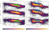 |
Fig. 13 Elemental abundance distribution of the sample in the [X/Fe]–[Fe/H] plane. Only stars with S/Nr > 100 are shown. The sample is separated into two temperature bins: Teff < 10 000 K (left) and Teff > 10 000 K (right). Coloured circles (with error bars where available) represent literature results from high-resolution spectroscopy used in Sect. 4.1, following the same colour scheme as Fig. 4. Grey dots represent the reference pattern of Classical Cepheids from Trentin et al. (2024). |
5.5 Abundance gradient
The metallicity gradient in the Milky Way disc is a key observational constraint on models of Galactic chemical evolution and disc formation (Chiappini et al. 1997). Studies using a range of tracers – from classical Cepheids to H II regions, open clusters, and field red giants – consistently reveal a negative gradient of roughly −0.04 to −0.06 dex kpc−1 (Genovali et al. 2014, and references therein). Classical Cepheids have been instrumental because their well-calibrated period–luminosity and period–metallicity relations yield robust measurements of the present-day gradient (Genovali et al. 2014; Trentin et al. 2023).
In the context of Galactic evolution, such a negative gradient is expected from an inside-out formation scenario where the inner regions experience more rapid star formation and chemical enrichment. As a result, these central parts become more metal-rich than the outer disc. While secular processes like radial migration tend to blur the gradient over time (Minchev et al. 2013), particularly in older stellar populations, our sample of early-type stars, representing a relatively young population, traces the current state of the disc.
The relationship between abundance and Galactocentric radius (RGC) is shown in Fig. 14 for stars with S/Nr > 50 near the mid-plane (|z| < −0.4 kpc). BHB candidates ([Fe/H] < −1.4 dex) and chemically peculiar artefacts ([Fe/H] > 0.65 dex) are excluded. The remaining sample is grouped into radial bins, each containing at least 50 stars. Abundance values and uncertainties are computed as the weighted mean and standard deviation within each bin. The solid lines represent linear fits to our sample, with slopes indicated in the lower-left corner. Dotted black lines show Galactic gradients for each element derived from Classical Cepheids (Trentin et al. 2024).
The derived slopes and zero-points agree well with those obtained from Classical Cepheids, except for an offset in [O/H] (the second row), as discussed in Sect. 5.4. The close agreement between the gradients from our LAMOST early-type star sample and those from Cepheids reinforces the reliability of our methodology and supports the idea that recent chemical enrichment of the disc has been spatially and temporally coherent.
Furthermore, the abundance spreads remain homogeneous within RGC ⩽ 10 kpc but increase significantly in the outer disc (RGC ⩾ 12 kpc), particularly for [Fe/H] and [Si/H]. This trend aligns with the larger scatter reported in Cepheids at greater distances (Trentin et al. 2023), suggesting that the interstellar medium becomes less homogeneous farther from the Galactic centre.
Trentin et al. (2023) identified a possible break in the gradient at RGC = 9.25 kpc, with slopes of −0.063 ± 0.007 dex kpc−1 and −0.079 ± 0.003 dex kpc−1 for the inner and outer regions, respectively. A similar trend is tentatively seen in [Fe/H], indicating a steeper gradient at larger distances. This consistency across different tracers and methods strengthens the interpretation that the observed gradient reflects the disc’s star formation history and dynamical evolution (but see also results from open clusters, e.g. Joshi et al. 2024).
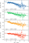 |
Fig. 14 Galactic radial gradients for [Fe/H], [O/H], [Mg/H], and [Si/H] (from top to bottom). Stars in the mid-plane (|z| < −0.4 kpc) with S/Nr > 50 are grouped into radial bins. Only bins containing at least 50 stars are shown, with values and uncertainties computed as the weighted mean and standard deviation of the abundances within each bin. The best-fit linear correlation is shown as a solid line, with its slope in the lower-left corner. The dotted line represents literature results for Galactic radial gradients derived from Classical Cepheids (Trentin et al. 2024). |
6 Summary
In this work, we present stellar parameters (Teff, log g, v sin i) and abundances of four elements (O, Mg, Si, and Fe) for 315 822 stars with S/N ⩾ 10 in the r-band from LAMOST DR9 low-resolution spectra. We combine two spectroscopic analysis approaches, SLAM and the Payne, to determine parameters for hot stars (Teff ~ 9500 K). The SLAM method, building on our prior work (Sun et al. 2021a,b; Sun & Chiappini 2024), demonstrates that stellar labels (particularly temperature and surface gravity) can be robustly derived from low- and medium-resolution spectra without excluding critical spectral features. Coupled with the Payne model, we extend this to abundance determinations for hot stars, offering new insights into massive star evolution and Galactic chemical enrichment.
Synthetic tests reveal improved precision in Teff and log g recovery at higher S/N, though performance declines for hotter stars. Abundance measurements show temperature-dependent scatter, with [C/Fe], [S/Fe], and [Ca/Fe] excluded due to large uncertainties and weak S/N trends. Repeat observations yield typical uncertainties of 163 K in Teff, 0.12 dex in log g, and 0.10 dex in [Fe/H], consistent with synthetic tests to within a factor of two.
We verified labels against high-resolution benchmarks spanning Teff ~ 8000–19 000 K and [Fe/H] ~−1.0 to 0.5 dex, including three giants. Results show good agreement for Teff, log g, and v sin i. Iron abundances match literature values but diverge at Teff > 15 000 K, with metal-poor stars underestimated. [Mg/Fe] and [Si/Fe] show the lowest scatter (σ ~ 0.3 dex), while [O/Fe] agrees moderately (σ ~ 0.4 dex). Comparisons with Xiang et al. (2022) and Sun et al. (2021a) reveal systematic offsets for stars with temperatures between 9000 and 11 000 K, likely from differences in Balmer-line treatment. Over 95% of the high-S/N sample satisfies photometric selection criteria from Zari et al. (2021), validating their utility for OBA-star identification.
We identify 3564 BHB candidates via metallicity ([Fe/H] ⩽ −1.4 dex) and Galactic latitude (|b| ⩾ 15°). Of these, 90% exhibit low log g (< 3.5 dex) and align with PARSEC horizontal-branch isochrones. A distinct subgroup (10%) with higher log g and moderate rotation (v sin i ~ 50 km s−1) likely represents blue stragglers. Discrepancies in log g with Xiang et al. (2022) highlight methodological differences.
Abundance trends for stars below 10 000 K align with the high-α sequence from Hayden et al. (2015), while hotter stars show steeper slopes and elevated [O/Fe] and [Mg/Fe], suggesting temperature-dependent systematics. We identify a super metal-rich population ([Fe/H] > 0.5 dex) with narrow [O/Fe] scatter and a low-α sequence in [O/Fe]–[Fe/H] and [Mg/Fe]–[Fe/H] planes.
Our results confirm a negative abundance gradient consistent with previous studies of Classical Cepheids, with a slope of −0.070 ± 0.007 in [Fe/H] over Galactocentric distances between 6 and 15 kpc. This reinforces the reliability of our methodology and supports the notion that recent chemical enrichment in the Milky Way disc has been spatially and temporally coherent. The abundance spread remains uniform within RGC ⩽ 10 kpc but increases significantly beyond 12 kpc, particularly in [Fe/H] and [Si/H], suggesting a less homogeneous interstellar medium at larger radii.
This catalogue establishes a foundation for studying Galactic hot stellar populations. Future work should incorporate NLTE modelling to address systematic offsets in [O/Fe] and [Mg/Fe] for rapidly rotating stars. Upcoming data releases SDSS-V (e.g. SDSS-V; Almeida et al. 2023) will enhance metal-poor samples where current deviations increase. Joint photometricspectroscopic analyses could resolve log g discrepancies for A-type stars via continuum constraints (e.g. Ju et al. 2025).
The synergy between SLAM and Payne frameworks demonstrates their adaptability for surveys like 4MOST (de Jong et al. 2019), and in particular, its 4MIDABLE-LR (Chiappini et al. 2019) consortium survey, enabling unified chemical inventories across stellar evolution stages. Such advances will be critical to improving our understanding of cosmic abundance variations and the role of massive stars in Galactic chemical evolution.
Data availability
The data underlying this article are available at the CDS via anonymous ftp to cdsarc.cds.unistra.fr (130.79.128.5) or via https://cdsarc.cds.unistra.fr/viz-bin/cat/J/A+A/698/A300
Acknowledgements
We are deeply grateful to C. Chiappini for the insightful discussions and comments. We thank the anonymous referee for their valuable comments. The Guoshoujing Telescope (the Large Sky Area Multi-Object Fibre Spectroscopic Telescope; LAMOST) is a National Major Scientific Project built by the Chinese Academy of Sciences. Funding for the project has been provided by the National Development and Reform Commission. LAMOST is operated and managed by the National Astronomical Observatories, Chinese Academy of Sciences. This work has made use of data from the European Space Agency (ESA) mission Gaia (https://www.cosmos.esa.int/gaia), processed by the Gaia Data Processing and Analysis Consortium (DPAC; https://www.cosmos.esa.int/web/gaia/dpac/consortium). Funding for the DPAC has been provided by national institutions, in particular the institutions participating in the Gaia Multilateral Agreement. Facility: LAMOST. Software: astropy (Astropy Collaboration 2013), IPython (Perez & Granger 2007), laspec (Zhang et al. 2021), matplotlib (Hunter 2007).
Appendix A Pixel-scale precision
To evaluate the spectroscopic precision of our model (particularly the Payne implementation), we compare interpolated synthetic spectra with original test models at S/N = 1000. Fig. A.1 displays flux residual distributions for all pixels (blue) and line-core pixels with fλ < 0.95 (green). The global pixel residual dispersion is 0.19% (equivalent to S/N ~ 500 per pixel), significantly smaller than typical LAMOST-LRS spectral errors. This precision persists when examining H-line cores, where the dispersion increases to 0.37% (S/N ~270) while remaining below observational uncertainties.
As Ting et al. (2017) demonstrated, gradient spectra ∇l – quantifying spectral response to parameter variations – reveal spectroscopic information content. Fig. A.2 compares our Payne-derived gradients with Kurucz model calculations for a reference star with Teff = 12500 K. We compute gradients by differencing spectra with parameter offsets: ΔTeff = 200 K, Δ log g = 0.2 dex, Δvmic = 4 km s−1, Δv sin i = 50 km s−1, and Δ[Fe/H] = Δ[X/Fe] = 0.2 dex. The Payne gradients for Teff = 12500 K show excellent agreement with Kurucz models. Broad continuum features near strong absorption lines arise from normalisation effects, while sharp variations trace line profile changes.
We additionally compare a hotter reference star (Teff = 17500 K; orange in Fig. A.2) while maintaining identical other parameters, applying a vertical offset for clarity. The most notable trend is the shallower gradient amplitude in hotter stars compared to their cooler counterparts. This manifests in ∇Teff and ∇ log g through reduced variations near hydrogen line cores (Fig. A.2), a pattern similarly observed in ∇[Fe/H] and ∇[X/Fe]. These diminished gradients imply temperature-dependent information loss: hotter stars’ spectra contain weaker abundance sensitivity at fixed noise levels. While our model successfully reproduces the input gradient spectra, we emphasise that their absolute amplitudes (< 2%) remain relatively flat compared to FGK stars. This information degradation intensifies with increasing temperature, underscoring the necessity for high-S/N (≳ 300) observations even at LAMOST-LRS resolution to reliably constrain atmospheric parameters.
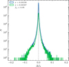 |
Fig. A.1 Distribution of flux residuals for 5000 test spectra at S/N = 1000. Standard deviations for all pixels (blue) and pixels with normalised flux fλ < 0.95 (green) are indicated in the top-left corner. The latter criterion selects line-core regions of strong absorption features. |
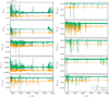 |
Fig. A.2 Gradient spectra ∇l for reference stars with Teff = 12500 K (blue) and Teff = 17500 K (orange) from Kurucz models, compared to Payne model predictions (green) for Teff = 12500 K. A vertical offset separates the gradients for the hotter star. Both stars share log g = 3.5 dex, vmic = 5 km s−1, v sin i = 150 km s−1, [Fe/H] = −0.4 dex, and solar abundances for other elements. |
References
- Almeida, A., Anderson, S. F., Argudo-Fernández, M., et al. 2023, ApJS, 267, 44 [NASA ADS] [CrossRef] [Google Scholar]
- Asplund, M., Grevesse, N., Sauval, A. J., et al. 2009, ARA&A, 47, 481 [Google Scholar]
- Astropy Collaboration (Robitaille, T. P., et al.) 2013, A&A, 558, A33 [NASA ADS] [CrossRef] [EDP Sciences] [Google Scholar]
- Bailer-Jones, C. A. L., Rybizki, J., Fouesneau, M., et al. 2021, AJ, 161, 147 [NASA ADS] [CrossRef] [Google Scholar]
- Blomme, R., Daflon, S., Gebran, M., et al. 2022, A&A, 661, A120 [NASA ADS] [CrossRef] [EDP Sciences] [Google Scholar]
- Bragança, G. A., Daflon, S., Lanz, T., et al. 2019, A&A, 625, A120 [NASA ADS] [CrossRef] [EDP Sciences] [Google Scholar]
- Bressan, A., Marigo, P., Girardi, L., et al. 2012, MNRAS, 427, 127 [NASA ADS] [CrossRef] [Google Scholar]
- Caffau, E., Ludwig, H.-G., Malherbe, J.-M., et al. 2013, A&A, 554, A126 [NASA ADS] [CrossRef] [EDP Sciences] [Google Scholar]
- Carraro, G., Vázquez, R. A., Costa, E., et al. 2010, ApJ, 718, 683 [Google Scholar]
- Chang, C., & Lin, C. 2011, ACM Trans. Intell. Syst. Technol. 2, 27 [CrossRef] [Google Scholar]
- Chiappini, C., Matteucci, F., & Gratton, R. 1997, ApJ, 477, 765 [Google Scholar]
- Chiappini, C., Minchev, I., Starkenburg, E., et al. 2019, The Messenger, 175, 30 [NASA ADS] [Google Scholar]
- Choi, J., Dotter, A., Conroy, C., et al. 2016, ApJ, 823, 102 [Google Scholar]
- Clewley, L., Warren, S. J., Hewett, P. C., et al. 2002, MNRAS, 337, 87 [NASA ADS] [CrossRef] [Google Scholar]
- de Jong, R. S., Agertz, O., Berbel, A. A., et al. 2019, The Messenger, 175, 3 [NASA ADS] [Google Scholar]
- Deng, L.-C., Newberg, H. J., Liu, C., et al. 2012, Res. Astron. Astrophys., 12, 735 [Google Scholar]
- Dunstall, P. R., Dufton, P. L., Sana, H., et al. 2015, A&A, 580, A93 [NASA ADS] [CrossRef] [EDP Sciences] [Google Scholar]
- Eldridge, J. J., & Stanway, E. R. 2022, ARA&A, 60, 455 [NASA ADS] [CrossRef] [Google Scholar]
- Gebruers, S., Straumit, I., Tkachenko, A., et al. 2021, A&A, 650, A151 [NASA ADS] [CrossRef] [EDP Sciences] [Google Scholar]
- Genovali, K., Lemasle, B., Bono, G., et al. 2014, A&A, 566, A37 [NASA ADS] [CrossRef] [EDP Sciences] [Google Scholar]
- Gray, R. O., & Corbally, C. 2009, Stellar Spectral Classification, eds. R. O. Gray & C. J. Corbally (Princeton University Press) [CrossRef] [Google Scholar]
- Guo, Y., Zhang, B., Liu, C., et al. 2021, ApJS, 257, 54 [NASA ADS] [CrossRef] [Google Scholar]
- Hayden, M. R., Bovy, J., Holtzman, J. A., et al. 2015, ApJ, 808, 132 [Google Scholar]
- Hobbs, L. M., York, D. G., Snow, T. P., et al. 2008, ApJ, 680, 1256 [NASA ADS] [CrossRef] [Google Scholar]
- Hunter, J. D. 2007, Comput. Sci. Eng., 9, 90 [NASA ADS] [CrossRef] [Google Scholar]
- Joshi, Y. C., Deepak, & Malhotra, S. 2024, Front. Astron. Space Sci., 11, 1348321 [NASA ADS] [CrossRef] [Google Scholar]
- Ju, J., Cui, W., Huo, Z., et al. 2024, ApJS, 270, 11 [Google Scholar]
- Ju, J., Zhang, B., Cui, W., et al. 2025, ApJS, 276, 12 [Google Scholar]
- Kingma, D. P., & Ba, J. 2014, arXiv e-prints [arXiv:1412.6980] [Google Scholar]
- Kinman, T. D., Suntzeff, N. B., & Kraft, R. P. 1994, AJ, 108, 1722 [Google Scholar]
- Kurucz, R. L. 2005, Mem. Soc. Astron. Ital. Suppl., 8, 14 [Google Scholar]
- Lanz, T., & Hubeny, I. 2007, ApJS, 169, 83 [CrossRef] [Google Scholar]
- Leiner, E., Mathieu, R. D., Gosnell, N. M., et al. 2018, ApJ, 869, L29 [NASA ADS] [CrossRef] [Google Scholar]
- Leonard, P. J. T., & Livio, M. 1995, ApJ, 447, L121 [NASA ADS] [CrossRef] [Google Scholar]
- Lian, J., Bergemann, M., Pillepich, A., et al. 2023, Nat. Astron., 7, 951 [CrossRef] [Google Scholar]
- Liu, X.-W., Yuan, H.-B., Huo, Z.-Y., et al. 2014, Setting the scene for Gaia and LAMOST, 298, 310 [Google Scholar]
- Liu, Z., Cui, W., Liu, C., et al. 2019, ApJS, 241, 32 [CrossRef] [Google Scholar]
- Luo, A.-L., Zhao, Y.-H., Zhao, G., et al. 2015, Res. Astron. Astrophys., 15, 1095 [Google Scholar]
- Maeder, A., & Conti, P. S. 1994, ARA&A, 32, 227 [NASA ADS] [CrossRef] [Google Scholar]
- Maiolino, R., & Mannucci, F. 2019, A&A Rev., 27, 3. [NASA ADS] [CrossRef] [Google Scholar]
- Minchev, I., Chiappini, C., & Martig, M. 2013, A&A, 558, A9 [CrossRef] [EDP Sciences] [Google Scholar]
- Morton, T. D. 2015, Astrophysics Source Code Library [record asc1:1503.010] [Google Scholar]
- Nissen, P. E., Chen, Y. Q., Carigi, L., et al. 2014, A&A, 568, A25 [NASA ADS] [CrossRef] [EDP Sciences] [Google Scholar]
- Paxton, B., Bildsten, L., Dotter, A., et al. 2011, ApJS, 192, 3 [Google Scholar]
- Pecaut, M. J., & Mamajek, E. E. 2013, ApJS, 208, 9 [Google Scholar]
- Perez, F., & Granger, B. E. 2007, Comput. Sci. Eng., 9, 21 [Google Scholar]
- Pier, J. R. 1984, ApJ, 281, 260 [Google Scholar]
- Przybilla, N., Butler, K., Becker, S. R., et al. 2006, A&A, 445, 1099 [NASA ADS] [CrossRef] [EDP Sciences] [Google Scholar]
- Przybilla, N., Nieva, M.-F., & Butler, K. 2011, J. Phys. Conf. Ser., 328, 012015 [Google Scholar]
- Puls, J., Vink, J. S., & Najarro, F. 2008, A&A Rev., 16, 209 [NASA ADS] [CrossRef] [Google Scholar]
- Reader, J., Corliss, C. H., Wiese, W. L., et al. 1980, Wavelengths and transition probabilities for atoms and atomic ions: Part 1. Wavelengths, part 2. Transition probabilities, NSRDS-NBS Vol. 68 [Google Scholar]
- Riello, M., De Angeli, F., Evans, D. W., et al. 2021, A&A, 649, A3 [NASA ADS] [CrossRef] [EDP Sciences] [Google Scholar]
- Royer, F., Zorec, J., & Gómez, A. E. 2007, A&A, 463, 671 [NASA ADS] [CrossRef] [EDP Sciences] [Google Scholar]
- Skrutskie, M. F., Cutri, R. M., Stiening, R., et al. 2006, AJ, 131, 1163 [NASA ADS] [CrossRef] [Google Scholar]
- Striganov, A.-R., & Sventitskii, N.-S. 2013, Tables of Spectral Lines of Neutral and Ionised Atoms (Springer Science & Business Media) [Google Scholar]
- Sun, W., & Chiappini, C. 2024, A&A, 689, A141 [NASA ADS] [CrossRef] [EDP Sciences] [Google Scholar]
- Sun, W., de Grijs, R., Deng, L., et al. 2019, ApJ, 876, 113 [NASA ADS] [CrossRef] [Google Scholar]
- Sun, W., Duan, X.-W., Deng, L., et al. 2021a, ApJS, 257, 22 [NASA ADS] [CrossRef] [Google Scholar]
- Sun, W., Duan, X.-W., Deng, L., et al. 2021b, ApJ, 921, 145 [NASA ADS] [CrossRef] [Google Scholar]
- Takahashi, K., & Langer, N. 2021, A&A, 646, A19 [NASA ADS] [CrossRef] [EDP Sciences] [Google Scholar]
- Takeda, Y., & Honda, S. 2016, PASJ, 68, 32 [NASA ADS] [CrossRef] [Google Scholar]
- Takeda, Y., Han, I.-W., Kang, D.-I., et al. 2008, J. Korean Astron. Soc., 41, 83 [NASA ADS] [CrossRef] [Google Scholar]
- Ting, Y.-S., Conroy, C., Rix, H.-W., et al. 2017, ApJ, 843, 32 [NASA ADS] [CrossRef] [Google Scholar]
- Ting, Y.-S., Conroy, C., Rix, H.-W., et al. 2019, ApJ, 879, 69 [NASA ADS] [CrossRef] [Google Scholar]
- Tkachenko, A. 2015, A&A, 581, A129 [NASA ADS] [CrossRef] [EDP Sciences] [Google Scholar]
- Trentin, E., Ripepi, V., Catanzaro, G., et al. 2023, MNRAS, 519, 2331 [Google Scholar]
- Trentin, E., Catanzaro, G., Ripepi, V., et al. 2024, A&A, 690, A246 [NASA ADS] [CrossRef] [EDP Sciences] [Google Scholar]
- Venn, K. A. 1995, ApJS, 99, 659 [NASA ADS] [CrossRef] [Google Scholar]
- Xiang, M., Ting, Y.-S., Rix, H.-W., et al. 2019, ApJS, 245, 34 [Google Scholar]
- Xiang, M., Rix, H.-W., Ting, Y.-S., et al. 2022, A&A, 662, A66 [NASA ADS] [CrossRef] [EDP Sciences] [Google Scholar]
- Xue, X. X., Rix, H. W., Zhao, G., et al. 2008, ApJ, 684, 1143 [Google Scholar]
- Zari, E., Rix, H.-W., Frankel, N., et al. 2021, A&A, 650, A112 [NASA ADS] [CrossRef] [EDP Sciences] [Google Scholar]
- Zhang, B., Liu, C., & Deng, L.-C. 2020a, ApJS, 246, 9 [NASA ADS] [CrossRef] [Google Scholar]
- Zhang, B., Liu, C., Li, C.-Q., et al. 2020b, Res. Astron. Astrophys., 20, 051 [CrossRef] [Google Scholar]
- Zhang, B., Li, J., Yang, F., et al. 2021, ApJS, 256, 14 [NASA ADS] [CrossRef] [Google Scholar]
- Zhao, G., Zhao, Y.-H., Chu, Y.-Q., et al. 2012, Res. Astron. Astrophys., 12, 723 [CrossRef] [Google Scholar]
- Zinnecker, H., & Yorke, H. W. 2007, ARA&A, 45, 481 [Google Scholar]
All Tables
All Figures
|
Fig. 1 Recovery precision for Teff (top) and log g (bottom) from the SLAM module across the Kiel diagram. Test spectra are binned by ΔTeff = 1000 K and Δ log g = 0.5 dex (delineated by dashed grey lines). For each bin with a significant number of spectra, the four ‘traffic light’ bullets show the standard deviation of the label for S/Ns of (top to bottom) 30, 50, 100, and 250. Empty bins contain insufficient data for robust statistics. |
| In the text | |
|
Fig. 2 Label recovery precision versus signal-to-noise ratio (S/N per Å) for the spectroscopic pipeline. Solid and dashed lines represent scatter (σ) and bias (μ), respectively, calculated within S/N bins. Coloured bands indicate three temperature regimes: 7000 K < Teff < 9000 K (blue), 9000 K < Teff < 13 000 K (green), and 13 000 K < Teff < 17 000 K (orange). Insets show σ and μ values at S/N = 100 in the units applicable to the respective labels for the full sample. |
| In the text | |
|
Fig. 3 Scatter of labels between repeated observations. The S/Nr is defined as the average value of the S/N in the r band of the observations, and the scatter Δrepl is the standard deviation of the labels in the units applicable to the respective labels, weighted by their S/N. Dashed orange lines represent the median value of the scatter in each S/N bin. Horizontal red lines indicate the median value of Δrepl from the entire sample with repeated observations, which are also marked in the top-right corner. |
| In the text | |
|
Fig. 4 Kiel diagram (top panel) and abundance patterns (bottom panel) for benchmark stars. Symbols denote different literature sources: Przybilla et al. (2006, orange), Takeda et al. (2008, green), and Gebruers et al. (2021, blue). Faded markers indicate stars lacking available spectra for direct verification. |
| In the text | |
|
Fig. 5 Label differences Δl = llit − l between literature results from high-resolution spectroscopy and this work, plotted against Teff. Coloured symbols denote benchmark stars with high-resolution data, where colour intensity corresponds to label values. Circles indicate stars with LAMOST LRS spectra, while empty squares represent spectra mimicked from high-resolution observations. Error bars and upper limits reflect uncertainties from Przybilla et al. (2006), Takeda et al. (2008), and Gebruers et al. (2021). |
| In the text | |
|
Fig. 6 Parameter comparisons with Xiang et al. (2022, LRS) and Sun et al. (2021a, MRS). Colour density scales with log(N). Panels b–c overlay contours (white) for 9000–11 000 K stars. Dashed lines show 1:1 relations, with red text indicating mean offsets (μ) and standard deviations (σ). |
| In the text | |
|
Fig. 7 Difference Δl = lXiang − l as a function of Teff from the SLAM module. Subplots from top to bottom show results for Teff, log g, [Fe/H], and v sin i, respectively. |
| In the text | |
|
Fig. 8 Distribution (N, top) and complementary cumulative distribution functions (ϕ, bottom) of v sin i for cross-matched samples in this work (blue), Sun et al. (2021a) (green), and Xiang et al. (2022) (orange). The dashed grey line at v sin i = 120 km s−1 marks the estimated lower threshold for a reliable v sin i determination at the LAMOST-LRS resolution. |
| In the text | |
|
Fig. 9 Distribution of candidate stars with r-band S/N > 10 in the Kiel diagram. Stellar density is colour-coded on a logarithmic scale. Temperature cuts at 7100 K and 19 000 K are applied. Stars above the dashed red line represent artefacts from intrinsically hotter stars (Teff ⩾ 20 000 K) and are excluded from further analysis. Grey curves show evolutionary tracks for stars with masses of 1.7, 2.0, 2.5, 3.0, 4.0, 5.0, and 7.0 M⊙ from MIST (Paxton et al. 2011; Choi et al. 2016) models. |
| In the text | |
|
Fig. 10 J − H vs G − Ks colour-–colour diagram (left) and G vs G − Ks colour-magnitude diagram (right) for the sample with S/N ⩾ 50. Stellar density is colour-coded on a logarithmic scale. Density contours derived from kernel density estimates are white for the entire sample. Dashed red lines and shaded grey areas delineate the selection criteria for OBA stars as outlined by Zari et al. (2021). |
| In the text | |
|
Fig. 11 Distribution of stars with S/Nr ⩾ 50 in [Fe/H] and v sin i space. The right subplot displays the logarithmic histogram distribution of [Fe/H], with a horizontal dashed line indicating the metallicity threshold ([Fe/H] = −1.4 dex) for the BHB candidate selection. |
| In the text | |
|
Fig. 12 3564 BHB candidates in the Kiel diagram, colour-coded by projected rotational velocities. Grey dots show BHB candidates selected by Xiang et al. (2022) using similar selection criteria. Red lines display PARSEC (Bressan et al. 2012) isochrones for horizontal branch stars with metallicities [Fe/H] = −2.5 dex (solid) and −2.0 dex (dashed), corresponding to ages log(t/yr = 8.6, 8.8, and 9.0 (left to right, respectively). |
| In the text | |
|
Fig. 13 Elemental abundance distribution of the sample in the [X/Fe]–[Fe/H] plane. Only stars with S/Nr > 100 are shown. The sample is separated into two temperature bins: Teff < 10 000 K (left) and Teff > 10 000 K (right). Coloured circles (with error bars where available) represent literature results from high-resolution spectroscopy used in Sect. 4.1, following the same colour scheme as Fig. 4. Grey dots represent the reference pattern of Classical Cepheids from Trentin et al. (2024). |
| In the text | |
|
Fig. 14 Galactic radial gradients for [Fe/H], [O/H], [Mg/H], and [Si/H] (from top to bottom). Stars in the mid-plane (|z| < −0.4 kpc) with S/Nr > 50 are grouped into radial bins. Only bins containing at least 50 stars are shown, with values and uncertainties computed as the weighted mean and standard deviation of the abundances within each bin. The best-fit linear correlation is shown as a solid line, with its slope in the lower-left corner. The dotted line represents literature results for Galactic radial gradients derived from Classical Cepheids (Trentin et al. 2024). |
| In the text | |
|
Fig. A.1 Distribution of flux residuals for 5000 test spectra at S/N = 1000. Standard deviations for all pixels (blue) and pixels with normalised flux fλ < 0.95 (green) are indicated in the top-left corner. The latter criterion selects line-core regions of strong absorption features. |
| In the text | |
|
Fig. A.2 Gradient spectra ∇l for reference stars with Teff = 12500 K (blue) and Teff = 17500 K (orange) from Kurucz models, compared to Payne model predictions (green) for Teff = 12500 K. A vertical offset separates the gradients for the hotter star. Both stars share log g = 3.5 dex, vmic = 5 km s−1, v sin i = 150 km s−1, [Fe/H] = −0.4 dex, and solar abundances for other elements. |
| In the text | |
Current usage metrics show cumulative count of Article Views (full-text article views including HTML views, PDF and ePub downloads, according to the available data) and Abstracts Views on Vision4Press platform.
Data correspond to usage on the plateform after 2015. The current usage metrics is available 48-96 hours after online publication and is updated daily on week days.
Initial download of the metrics may take a while.