| Issue |
A&A
Volume 673, May 2023
|
|
|---|---|---|
| Article Number | A155 | |
| Number of page(s) | 36 | |
| Section | Galactic structure, stellar clusters and populations | |
| DOI | https://doi.org/10.1051/0004-6361/202245399 | |
| Published online | 24 May 2023 | |
StarHorse results for spectroscopic surveys and Gaia DR3: Chrono-chemical populations in the solar vicinity, the genuine thick disk, and young alpha-rich stars⋆
1
Leibniz-Institut für Astrophysik Potsdam (AIP), An der Sternwarte 16, 14482 Potsdam, Germany
e-mail: This email address is being protected from spambots. You need JavaScript enabled to view it.
2
Institut für Physik und Astronomie, Universität Potsdam, Haus 28 Karl-Liebknecht-Str. 24/25, 14476 Golm, Germany
3
Laboratório Interinstitucional de e-Astronomia – LIneA, Rua Gal. José Cristino 77, Rio de Janeiro, RJ, 20921-400
Brazil
4
Dept. de Física Quàntica i Astrofísica (FQA), Universitat de Barcelona (UB), C Martí i Franqués, 1, 08028 Barcelona, Spain
5
Institut de Ciències del Cosmos (ICCUB), Universitat de Barcelona (UB), C Martí i Franqués, 1, 08028 Barcelona, Spain
6
Institut d’Estudis Espacials de Catalunya (IEEC), C Gran Capità, 2-4, 08034 Barcelona, Spain
7
Instituto de Física, Universidade Federal do Rio Grande do Sul, Caixa Postal 15051, Porto Alegre, RS, 91501-970
Brazil
8
Instituto de Astrofísica de Canarias, 38205 La Laguna, Tenerife, Spain
9
Departamento de Astrofísica, Universidad de La Laguna, 38200 La Laguna, Tenerife, Spain
10
Department of Astronomy, Universidade de São Paulo, São Paulo, 05508-090
Brazil
11
Instituto de Astronomía, Universidad Nacional Autónoma de México, A. P. 106, CP 22800 Ensenada BC, Mexico
12
Instituto de Astronomía, Universidad Católica del Norte, Av. Angamos 0610, Antofagasta, Chile
13
Centro de Investigación en Astronomía, Universidad Bernardo O’Higgins, Avenida Viel 1497, Santiago, Chile
14
Centro de Astronomía, Universidad de Antofagasta, Avenida Angamos 601, Antofagasta, 1270300
Chile
Received:
7
November
2022
Accepted:
15
March
2023
Abstract
The Gaia mission has provided an invaluable wealth of astrometric data for more than a billion stars in our Galaxy. The synergy between Gaia astrometry, photometry, and spectroscopic surveys gives us comprehensive information about the Milky Way. Using the Bayesian isochrone-fitting code StarHorse, we derive distances and extinctions for more than 10 million unique stars listed in both Gaia Data Release 3 and public spectroscopic surveys: 557 559 in GALAH+ DR3, 4 531 028 in LAMOST DR7 LRS, 347 535 in LAMOST DR7 MRS, 562 424 in APOGEE DR17, 471 490 in RAVE DR6, 249 991 in SDSS DR12 (optical spectra from BOSS and SEGUE), 67 562 in the Gaia-ESO DR5 survey, and 4 211 087 in the Gaia RVS part of the Gaia DR3 release. StarHorse can increase the precision of distance and extinction measurements where Gaia parallaxes alone would be uncertain. We used StarHorse for the first time to derive stellar ages for main-sequence turnoff and subgiant branch stars, around 2.5 million stars, with age uncertainties typically around 30%; the uncertainties drop to 15% for subgiant-branch-only stars, depending on the resolution of the survey. With the derived ages in hand, we investigated the chemical-age relations. In particular, the α and neutron-capture element ratios versus age in the solar neighbourhood show trends similar to previous works, validating our ages. We used the chemical abundances from local subgiant samples of GALAH DR3, APOGEE DR17, and LAMOST MRS DR7 to map groups with similar chemical compositions and StarHorse ages, using the dimensionality reduction technique t-SNE and the clustering algorithm HDBSCAN. We identify three distinct groups in all three samples, confirmed by their kinematic properties: the genuine chemical thick disk, the thin disk, and a considerable number of young alpha-rich stars (427) that are also a part of the delivered catalogues. We confirm that the genuine thick disk’s kinematics and age properties are radically different from those of the thin disk and compatible with high-redshift (z ≈ 2) star-forming disks with high dispersion velocities. We also find a few extra chemical populations in GALAH DR3 thanks to the availability of neutron-capture element information.
Key words: stars: abundances / Galaxy: disk / solar neighborhood / Galaxy: general / methods: statistical / Galaxy: stellar content
Data are only available at the CDS via anonymous ftp to cdsarc.cds.unistra.fr (130.79.128.5) or via https://cdsarc.cds.unistra.fr/viz-bin/cat/J/A+A/673/A155
© The Authors 2023
 Open Access article, published by EDP Sciences, under the terms of the Creative Commons Attribution License (https://creativecommons.org/licenses/by/4.0), which permits unrestricted use, distribution, and reproduction in any medium, provided the original work is properly cited.
This article is published in open access under the Subscribe to Open model. This email address is being protected from spambots. You need JavaScript enabled to view it. to support open access publication.
1. Introduction
The European Space Agency (ESA) Gaia mission (Gaia Collaboration 2016) is continuing to revolutionise and transform Galactic astrophysics in many areas (Brown 2021). The latest release from the Gaia mission, Data Release (DR) 3 (Gaia Collaboration 2023), is built upon the Early Data Release 3 (EDR3; Gaia Collaboration 2021). The EDR3 includes 36 months of observations, with positions and photometry for 1.7 × 10⁹ sources and full astrometric solutions (Lindegren et al. 2021) for 1.3 × 10⁹ objects. Gaia DR3 extends EDR3 by delivering multiple data products, for example low-resolution BP/RP spectra and astrophysical parameters for about 400 million sources (Andrae et al. 2023) and about 5 million sources with medium resolution spectra observed with the Radial Velocity Spectrometer (RVS) instrument (Recio-Blanco et al. 2023). Combining astrometric solutions from Gaia with large-scale spectroscopic surveys is fundamental for Galactic archaeology because it enables us to access the full phase space and the chemical composition of millions of stars. Such a rich trove of information gives us essential clues as to the formation and evolutionary history of the Milky Way (Freeman & Bland-Hawthorn 2002; Matteucci 2001, 2021; Pagel 2009), allowing us to disentangle the multiple overlapping processes that once took place in our Galaxy, such as mergers, secular evolution, and gas accretion flows.
The synergy between astrometry and spectroscopy resulted in many important discoveries in different components of our Galaxy. For example, we have the characterisation of the halo and the discovery of several accreted dwarf galaxies (e.g. Koppelman et al. 2018; Mackereth et al. 2019; Myeong et al. 2019; Limberg et al. 2021; Fernández-Trincado et al. 2020a,b, 2022; Horta et al. 2021; Ruiz-Lara et al. 2022) and the massive Gaia-Enceladus merger event (Haywood et al. 2018; Helmi et al. 2018; Belokurov et al. 2018). These structures substantially influence the formation of the thick disk and halo (for a review, see Belokurov et al. 2018; Di Matteo et al. 2019; Helmi 2020). The chemical duality of the Galactic disk, which is primarily evident in [α/Fe] versus [Fe/H] ratios in the solar neighbourhood, was shown by several authors to designate the chemical thin and thick disks (Adibekyan et al. 2011; Bensby et al. 2014; Anders et al. 2014; Hayden et al. 2015). Further, Rojas-Arriagada et al. (2019) and Queiroz et al. (2020) show that the same chemical bimodality extends to the inner Galaxy, indicating populations with different formation paths. Finally, the characterisation of the Galactic bulge and bar (Bovy et al. 2019; Lian et al. 2020; Rojas-Arriagada et al. 2020; Queiroz et al. 2021) in its chemo-orbital space reveals a diversity of populations coexisting in the inner Galaxy. Recently works that studied the inner Galaxy’s metal-poor counterpart show evidence of a pressure-supported component that follows a more spherical distribution than the disk and little to no rotation (Kunder et al. 2020; Arentsen et al. 2020; Lucey et al. 2021; Rix et al. 2022).
Achieving all the aforementioned scientific results is essential for calculating precise distances from the astrometric solutions provided by Gaia. As shown by Bailer-Jones (2015), determining distances by inverting the parallax is a limited and risky approach, especially for high astrometric uncertainties and large volumes of the Galaxy. In Queiroz et al. (2018, hereafter Q18), we presented the StarHorse code: a Bayesian isochrone fitting tool that makes versatile use of spectroscopic, photometric, and astrometric data to determine the distances, extinctions, and stellar parameters of field stars. The method was then extensively validated using simulations and external catalogues of asteroseismology, open clusters (OCs), and binaries. Therefore, in Queiroz et al. (2020, hereafter Q20) a great effort was made to provide catalogues generated from StarHorse using Gaia DR2 data with Apache Point Observatory Galactic Evolution Experiment (APOGEE) DR16 and other spectroscopic surveys, resulting in an important leap forwards in stellar parameter precision.
In this paper we provide updated StarHorse stellar parameters, distances, and extinctions for major spectroscopic surveys (see Table 1) combined with the Gaia DR3 data. The StarHorse results for APOGEE DR17 (Abdurro’uf et al. 2022) are already published in the form of a value-added catalogue (VAC) jointly with Sloan Digital Sky Survey (SDSS) DR17, except for the ages, which are published here for the first time. This paper focusses on science enabled by sub-samples for which StarHorse delivers reasonable age estimates thanks to the exquisite quality of the Gaia parallaxes. However, the results are limited to a local volume bubble of d < 2 kpc since ages derived via isochronal matching can only be reliable for the main sequence turnoff (MSTO) and subgiant branch (SGB) regimes, the degeneracies between neighbouring isochrones in the Hertzsprung-Russell diagram being much smaller for these cases.
Summary of the datasets for which we deliver StarHorse parameters in this work.
In this work we take advantage of the rich chemical information delivered by spectroscopic surveys combined with StarHorse ages to explore the detection of known and newly discovered chrono-chemical subgroups more in the line of classical ‘chemical tagging’ (see e.g. Freeman & Bland-Hawthorn 2002; Anders et al. 2018; Buder et al. 2022). To this aim, we used three different survey samples to map groups with similar chemical compositions.
This paper is outlined as follows. In Sect. 2 we summarise the Bayesian techniques used in StarHorse, the references for its newest implementations, and its main configuration. In Sect. 3 we describe the datasets we used as input to the StarHorse code as well as the astrometric, photometric, and spectroscopic data. In Sect. 4 we discuss the main parameters derived with our method, the newly released StarHorse catalogues, which contain more than 10 million stars (including 2.5 million nearby stars with ages), and a few validations of the parameters. In Sect. 5 we show relations between the derived ages and some chemical relations. In Sect. 6 we show our results using the chemo-age multi-dimension in the t-distributed stochastic neighbour embedding (t-SNE) technique and Hierarchical Density-Based Spatial Clustering of Applications with Noise (HDBSCAN) algorithm. Finally, in Sect. 7 we present our new conclusions and summarise our main results. All the catalogues used in this work are made public in the Leibniz Instititute für Astrophysik (AIP) database1.
2. Method
Isochrone fitting has been extensively used in astronomy to indirectly derive unknown stellar parameters by using known measured stellar properties (e.g. Pont & Eyer 2004; Jørgensen & Lindegren 2005; da Silva et al. 2006; Naylor & Jeffries 2006). A diversity of methods can be applied to the fitting procedure, (e.g. Burnett & Binney 2010; Rodrigues et al. 2014; Santiago et al. 2016, hereafter S16; Mints & Hekker 2018; Das & Sanders 2019; Lebreton & Reese 2020; Souza et al. 2020). Here we use StarHorse (S16; Q18; Q20; Anders et al. 2019, 2022), a Bayesian isochrone-fitting code that has been optimised for heterogeneous input data (including spectroscopy, photometry, and astrometry). Its results are limited only by observational errors and the accuracy of the adopted stellar evolution models.
StarHorse is able to derive distances, d, extinctions, AV (at λ = 542 nm), ages, τ, masses, m*, effective temperatures, Teff, metallicities, [M/H], and surface gravities, log g. The resulting parameter uncertainties are directly linked with the set of observables used as input. A complete set of observables comprises multi-band photometry (from blue to mid-infrared wavelengths), parallax, log g, Teff, [M/H], and an extinction prior AV. In this work, we use all this information by combining data from public spectroscopic surveys with photometric surveys and Gaia parallaxes. We then execute the Bayesian technique to quantitatively match the observable set with stellar evolutionary models from the PAdova and TRiestre Stellar Evolution Code (PARSEC; Bressan et al. 2012), ranging from 0.025 to 13.73 Gyr in age and −2.2 to +0.6 in metallicity.
Since Q20, StarHorse has seen several upgrades that are explained in Sect. 3 of Anders et al. (2022). These upgrades include the implementation of extragalactic and globular cluster priors, a change in the bar-angle prior (to the canonical value of 27°; e.g. Bland-Hawthorn & Gerhard 2016), a new three-dimensional extinction prior, and updated evolutionary models that include diffusion (especially important during the evolutionary phases close to the MSTO). Finally, the new catalogues presented here also take advantage of the more precise and additional data products of Gaia DR3.
3. Input data
The large set of available spectroscopic surveys gives us detailed information about individual stars, such as chemical abundances, atmospheric parameters, and radial velocities. By combining this information with photometry and astrometry, we can constrain models by a small range of limits and effectively derive the best fitting StarHorse parameters with low uncertainties.
We followed a very similar approach to previous StarHorse papers (Q18,Q20). In Table 1, we summarise the input numbers of stars for each spectroscopic survey, the stars remaining after applying a few quality cuts, the resulting number of converged stars, and the following amount of MSTO and SGB stars with available StarHorse ages. The quality cuts applied before executing StarHorse vary from survey to survey, and a more detailed explanation is given in the following subsections. As regard to model grid resolution and the photometric passband that we used as the ‘bestfilter’ are also described in the lower rows of Table 1. The agestep and metstep represent the spacing between age and metallicity in the models we use in the StarHorse method, for all cases the agestep is linear; for higher resolution surveys, we use a thinner model grid. The bestfilter is the primary choice from which we draw the possible distance values (for more information, see Sect. 3.2.1 of Q18).
In Fig. 1 we show the sky distribution for all public spectroscopic surveys for which derive StarHorse parameters; the area coverage of the surveys is very complementary and focusses on the different components of our Galaxy. Below, we summarise the configurations and calibrations done to all input data as well as the spectroscopic surveys and the photometric and astrometric catalogues used in this work.
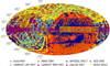 |
Fig. 1. Sky distribution of all public spectroscopic surveys for which we derive StarHorse parameters. |
3.1. Astrometric and photometric input
Gaia is an astrometric and photometric space mission from ESA launched in 2013. Since then it has delivered parallaxes and proper motions for more than 1 billion sources. Its EDR3 (Gaia Collaboration 2021) has astrometric solutions with uncertainties lower by half compared to its previous DR2 release. All resulting catalogues given in this paper were produced by combining the spectroscopic surveys with parallaxes from Gaia EDR3, which is an important new ingredient for the resulting StarHorse distances. We use the parallax corrections advertised by Lindegren et al. (2021), and the most conservative parallax uncertainty inflation factor derived in the analysis of Fabricius et al. (2021, see their Fig. 19). Besides these corrections, we crossmatched our catalogues with the fidelity_v1 column from Rybizki et al. (2022), which provides a scalar indicator for astrometric quality. For fidelities < 0.5, we do not use any parallax information. In the last column of the lower rows of Table 1 we show the coverage percentage of available parallaxes for the input catalogues that pass this condition.
As photometric input, we use infra-red photometry from Two Micron All Sky Survey (2MASS; Cutri et al. 2003) JHKs and unblurred coadds of the Wide-field Infrared Survey Explorer (unWISE; Schlafly et al. 2019) W1W2, optical data from the Panoramic Survey Telescope and Rapid Response System (Pan-STARRS-1; Scolnic et al. 2015) grizy, and SkyMapper Southern Sky Survey DR2 (Onken et al. 2019) griz, adopting generous minimum photometric uncertainties (between 0.03 and 0.08 mag). Magnitude shifts were applied to Pan-STARRS-1 as in Q20 using the values from Scolnic et al. (2015) and shift corrections were also applied to SkyMapper passbands according to Huang et al. (2021).
3.2. Spectroscopic catalogues
We computed posterior ages, masses, temperatures, surface gravities, distances, and extinctions for eight spectroscopic stellar surveys. We crossmatched all spectroscopic surveys with Gaia EDR3 using the stilts CDS-skymatch tool2. We used a 1.5 arcsec search radius for this, and with the setup as ‘find = each’ this configuration set the best match (best distance) for each row or blank when there was no match. We did not use any previous Gaia cross-matches made by the spectroscopic surveys with their sources since we can be consistent between our results by doing our own crossmatch. The photometric surveys such as Pan-STARRS and SkyMapper, which are already crossmatched with Gaia at the Gaia archive, are downloaded by their source id. For unWISE, we crossmatched all surveys with the same configuration as Gaia in the stilts CDS-skymatch tool. For all catalogues, we used the Salaris et al. (1993) transformation between [Fe/H] and [M/H] for stars with valid [α/Fe] values. For those without a reported [α/Fe] ratio, we assumed [M/H] ≃ [Fe/H]. The data curation applied for each survey is explained in the following subsections and the resulting numbers of stars are given in Table 1. We want to clarify that from each survey’s uncertainty distribution, we usually remove a small fraction with substantial input observable uncertainties compared to the full distribution. We do so because it is computationally very costly to calculate the likelihood for many models inside an extensive uncertainty range. The threshold of acceptable uncertainties to StarHorse changes with the choice of the model grid – high-resolution surveys typically have minor uncertainties, requiring a denser model grid.
3.2.1. APOGEE DR17
DR17 (Abdurro’uf et al. 2022) is the final data release of the fourth phase of the SDSS (SDSS IV; Blanton et al. 2017). It contains the complete APOGEE catalogue (Majewski et al. 2017) survey, which in December 2021 publicly released near infra-red spectra of over 650 000 stars. The APOGEE survey has been collecting data in the northern hemisphere since 2011 and the southern hemisphere since 2015. Both hemispheres observations use the twin near-infrared spectrographs with high resolution (R ≈ 22 500; Wilson et al. 2019) on the SDSS 2.5-m telescope at Apache Point Observatory (Gunn et al. 2006) and the 2.5-m du Pont telescope at Las Campanas Observatory (LCO; Bowen & Vaughan 1973). The data reduction pipeline is described in Nidever et al. (2015). The processed products of APOGEE DR17 are similar to the previous releases (Abolfathi et al. 2018; Holtzman et al. 2018; Jönsson et al. 2020). We use the temperature, surface gravity and metallicity results from the APOGEE Stellar Parameters and Abundances Pipeline (ASPCAP; García Pérez et al. 2016; Jönsson et al. 2020) to produce a new StarHorse catalogue as in Q20. We use primarily the calibrated parameters indicated in the pipeline, when those are not available we use spectroscopic parameters. For DR17 new synthetic spectral grids were added in ASPCAP, which also account for non-local thermodynamic equilibrium (non-LTE) in some elements. This led to the adoption of a different spectral synthesis code Synspec (Hubeny & Lanz 2017). Parameters reduction is also available with the previous spectral synthesis code TurboSpectrum (Alvarez & Plez 1998) but in StarHorse we only used the given parameters from Synspec. In Appendix B we show some differences between the derived abundances in Synspec and TurboSpectrum, which are discussed later in the analysis.
As an input to StarHorse, we selected only stars with available H2MASS passband and spectral parameters (FPARAM Abdurro’uf et al. 2022; Adibekyan et al. 2013)3, which reduces the total number of objects in the initial catalogue from 733 901 to 720 970. We then run StarHorse with a fine model grid (defined in age and metallicity steps, see the lower rows of Table 1). 22% of the input did not converge to a solution, meaning that these stars were incompatible with any stellar evolutionary model in our grid. The results for StarHorse using the data from APOGEE DR17 are also published in form of a VAC in Abdurro’uf et al. (2022).
3.2.2. GALAH DR3
The Galactic Archaeology with HERMES (GALAH) survey (De Silva et al. 2015; Martell et al. 2017) is a high-resolution spectroscopic survey that covers mostly a local volume, d < ≈2 kpc. Their latest data release, GALAH DR3, was published in November 2020. GALAH data are acquired with the High Efficiency and Resolution Multi-Element Spectrograph (HERMES), where the light is dispersed at R ≈ 28 000, coupled to the 3.9-m Anglo-Australian Telescope (AAT). HERMES observes in four different wavelengths simultaneously: blue (471.5−490.0 nm), green (564.9−587.3 nm), red (647.8−673.7 nm), and infrared (758.5−788.7 nm). We used the recommended catalogue, which contains radial velocities, atmospheric parameters, and abundances for a total of 588 571 stars (Buder et al. 2021). The stellar parameters are derived using the spectrum synthesis code Spectroscopy Made Easy (SME) and one-dimensional MARCS model atmospheres (Piskunov & Valenti 2017). GALAH makes available abundances for around 30 different elements, which cover five different nucleosynthetic pathways (α-process elements mostly formed by core-collapse supernovae (SNe), iron-peak elements formed mainly in type-Ia SNe, s-process elements formed in the late-life stage of low-mass stars, r-process elements formed by the merging of neutron stars, as well as lithium (created by the Big Bang and both created and destroyed in stars; Kobayashi et al. 2020). To derive StarHorse parameters, we selected only stars with mutually available Teff, log g and K2MASS passband as input. The coverage of high quality Gaia parallaxes for this sample is very high since most stars are nearby. Therefore, the resulting distances have very low uncertainties, as seen in Fig. 2. For GALAH, we ran StarHorse with a fine model grid, given the high resolution of the survey, and only 5% of the input catalogue did not converge.
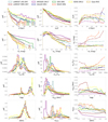 |
Fig. 2. Uncertainty distributions for StarHorse results. Left and middle panels: probability density functions of StarHorse output parameters and their respective uncertainties. The distributions are shown for each spectroscopic survey separately, as indicated in the legend. The upper panels, which show the distance and extinction, have their y-axis in logarithm scale to show the extent to larger values. Right panels: median trend of the dependence of each parameter with its associated uncertainty. |
3.2.3. LAMOST DR7
The Large Sky Area Multi-Object Fiber Spectroscopic Telescope (LAMOST; Cui et al. 2012; Zhao et al. 2012) is a spectroscopic survey covering a large area of the northern hemisphere, including stars and galaxies. LAMOST stellar parameter catalogues can be divided into LAMOST low resolution (LRS) and medium resolution (MRS). LAMOST, DR7, has been publicly available since March 2020 and includes the spectra obtained from the pilot survey through the seventh-year regular survey. We downloaded the stellar parameter catalogues for both LRS (6 179 327) and MRS (738 025)4. A new LAMOST data release, DR8, has been available since September 2022 and contains circa 500 000 new observations in LRS and 500 000 more in MRS. We will also make StarHorse parameters publicly available for this data release in the near future, but LAMOST DR8 is not part of the analysis in this paper.
Both MRS and LRS stellar parameter catalogues provide atmospheric parameters, metallicity, and projected rotation velocity estimated by the LAMOST Stellar Parameter Pipeline (LASP; Wu et al. 2014), as well as an estimate of alpha abundances by the method of template matching based on the MARCS synthetic spectra (Decin et al. 2004). For LAMOST MRS, co-added and single exposure spectra have a resolution of R ≈ 7500. The label-transfer method of Stellar Parameters and Chemical Abundances Network (SPCANet; Wang et al. 2020) gives 12 individual element abundances based on a convolutional neural network (CNN). For the MRS stellar parameter catalogue we selected all stars with mutually available log g, Teff, and 2MASS Ks photometry, and made the following cuts in uncertainty: σTeff < 300 K; σlog g < 0.5 K; σ[Fe/H] < 0.3 K. This left us with 457 359 stars as StarHorse input. As we did for the high-resolution surveys, we ran LAMOST MRS with the fine model grid, which led to a convergence rate of 93%. The LAMOST LRS parameter catalogue, the largest dataset in this work, consists of A, F, G, and K type stars. We selected stars with available log g, Teff, and 2MASS Ks passband and made the following cuts in uncertainty: σTeff < 500 K; σlog g < 0.8 K; σ[Fe/H] < 0.5 K, resulting in 4 803 496 stars as input. Using a coarsely spaced grid of models for LAMOST LRS, StarHorse was able to deliver results for 80% of this input catalogue.
3.2.4. SDSS DR12/SEGUE
The Sloan Extension for Galactic Understanding and Exploration (SEGUE; Yanny et al. 2009) is a spectroscopic survey that was conducted with the Sloan Foundation 2.5 m Telescope (Gunn et al. 2006) using the two original low-resolution SDSS fibre spectrographs (R ≈ 2000, Smee et al. 2013). The surveys targeted mostly metal-poor halo and disk stars. The stellar parameters from optical stellar spectra collected with SDSS/SEGUE were processed through the SEGUE Stellar Parameter Pipeline (SSPP), which reports three primary stellar parameters, Teff, log g, and metallicity. Most stars have Teff in the range between 4000 and 10 000 K and spectral signal-to-noise ratios greater than 10 (Lee et al. 2008; Allende-Prieto et al. 2008). In the final data release (SDSS DR12; Alam et al. 2015), the pipeline also provided [α/Fe] abundance ratios (Lee et al. 2011). From this catalogue, we use the recommended adopted values for Teff, log g and [Fe/H], selecting only stars with signal-to-noise ratios greater than 20 and that have all of these parameters available.
3.2.5. GES DR5
The Gaia-ESO Survey (GES; Gilmore 2012) targets > 105 stars in all major components of the Milky Way and OCs of all ages and masses. The survey conducted its observations with the Fibre Large Array Multi Element Spectrograph (FLAMES; Pasquini et al. 2002), which feeds two different instruments covering the whole visual spectral range. The fifth and final data release of GES was made public in May 2022 (Randich et al. 2022). It has significantly increased the number of observed stars, 114 324, about four times the size of the previous public release, and it also increased the number of derived abundances and cluster parameters. Several working groups focussing on different types of stars and evolutionary stages analysed the GES spectra (Heiter et al. 2021). We downloaded the full catalogue5, and used the recommended homogenised atmospheric parameters as StarHorse input. We only used entries with errors smaller than 300 K in temperature, 0.5 dex in surface gravity, and 0.6 dex in iron abundance. To correct the metallicities for the solar scale using the Salaris et al. (1993) formula, we calculated a global [α/Fe] estimate based on the abundances of Si, Ca, and Mg, available for about 58% of the stars in the catalogue. Compared to the previous StarHorse run on GES data, this is an important update because there are many more stars, and we do not exclude the OCs from our analysis any longer.
3.2.6. RAVE DR6
The final data release of the RAdial Velocity Experiment (RAVE; Steinmetz et al. 2006) survey, DR6 (Steinmetz et al. 2020), became public in 2020. The spectra from RAVE is acquired with the multi-object spectrograph deployed on 1.2-m UK Schmidt Telescope of the Australian Astronomical Observatory (AAO). The spectra have a medium resolution of R ≈ 7500 and cover the CaII-triplet region (8410−8795 Å). We use the final RAVE data release and in particular, the purely spectroscopically derived stellar atmospheric parameters subscripted cal_madera. In Q20 we explain the processing of this final RAVE data release in detail and we follow the same procedure for pre-processing this catalogue. The only difference is that this catalogue is now cross-matched with Gaia EDR3 instead of DR2.
3.2.7. Gaia DR3 RVS
Besides its photometric and astrometric instruments, Gaia also features a spectroscopic facility, the RVS. The instrument observes in the near-infrared (845−872 nm) and has a resolution of λ/Δλ ≈ 11 500 (Cropper et al. 2018). The third data release of Gaia contains data of the first 36 months of RVS observations, obtained with the General Stellar Parametriser from the Spectroscopy (GSP-Spec; Recio-Blanco et al. 2023) module of the Astrophysical parameters inference system (Apsis; Creevey et al. 2023). There are two analysis workflows to process these data: the MatisseGauguin pipeline and an artificial neural network (Recio-Blanco et al. 2016). We work here only with the data analysed by MatisseGauguin, which provides the stellar atmospheric parameters and individual chemical abundances of N, Mg, Si, S, Ca, Ti, Cr, Fe I, Fe II, Ni, Zr, Ce, and Nd for about 5.6 million stars (Recio-Blanco et al. 2023). We downloaded the data from the Gaia archive’s DR3 table of astrophysical parameters. Following a similar procedure to the other spectroscopic surveys, we combine the data with zero point-corrected parallaxes from Gaia EDR3, and with broad-band photometric data. We do not apply any quality flag cuts when running StarHorse, but we only select stars with acceptably small nominal uncertainties (σTeff < 700 K, σlog g < 1.0 dex, σ[Fe_H] < 0.6 dex). We also removed stars with [Fe_H] < −3, since those fall outside the metallicity range covered by the PARSEC stellar model grid used. Regarding parameter calibrations, we applied the suggestions for the calibration of log g, [M/H] and [α/Fe] detailed in Recio-Blanco et al. (2023).
4. New StarHorse catalogues
We present a new catalogue set derived from the stellar spectroscopic surveys described in Sect. 3.2 combined with photometry and Gaia EDR3 parallaxes (Sect. 3.1). We provide percentiles of the posterior distribution functions of masses, effective temperatures, surface gravities, metallicities, distances, and extinctions for each successful converged source according to Table 1. We deliver the final data in the same format as in Q20 Table A.1 for each spectroscopic survey used as input. The median value, 50th percentile, should be taken as the best estimate for that given quantity, and the uncertainty can be determined using the 84th and 16th percentiles. In this release, we also make for the first time age determinations for a selection of MSTO and SGB (MSTO+SGB) stars. The given ages follow the same format as the other StarHorse parameters, but we flag everything outside our MSTO+SGB selection as −999. All the newly produced StarHorse catalogues are available for download from6 and through VizieR. Some of the results of StarHorse for APOGEE, GALAH and SDSS DR12 have already been analysed by recent publications on the study of halo debris (Limberg et al. 2021, 2022a; Perottoni et al. 2022).
4.1. StarHorse distances and extinctions
Precise distances and extinctions are fundamental for Galactic archaeology (Helmi 2020). By combining spectroscopic and Gaia data, StarHorse achieves precise distances from the inner to the outer Galaxy. As seen in the left panels of Fig. 2 we get relative errors in the distance of only 15% for distances as far as 20 kpc, and a mean extinction uncertainty of about 0.2 (mag). Distances and extinctions have also been extensively validated with simulations and external methods in Q18 and Q20, showing internal precision in the distance and extinctions of about 8% and 0.04 mag, respectively. In Fig. 3 we show the distribution of stars for all surveys for which we compute distances in Galactocentric Cartesian coordinates. This map expresses the extent and capability of the resulting data, which samples very well the solar vicinity, reaches the inner parts of the Galaxy, covers the outer disk beyond RGal = 20 kpc and extends to |ZGal|> 10 kpc. We display the distribution of parameters and their uncertainties in Fig. 2, and we show the mean uncertainty in each parameter for each survey in Table 2. The mean relative distance uncertainty for all surveys lies below 10%, while for GALAH, APOGEE, LAMOST MRS and Gaia DR3 RVS, it is below 5%. It is noticeable from Fig. 2 that, with the new prior implementation (Anders et al. 2022), some survey distances extend to other galaxies; for example, APOGEE reaches the Magellanic Clouds, the Sagittarius dwarf galaxy, and some globular clusters. The AV value varies primarily according to each survey’s selection function, and its uncertainty is strongly correlated with photometry, but on average below 0.2 mag. For the most precise determinations of AV, one can select the stars with the complete photometry input set (detailed in the StarHorse input flags).
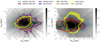 |
Fig. 3. Galactic distribution of all spectroscopic surveys for which we present StarHorse results in this paper. The grey background density shows the star counts for all surveys combined, while the coloured bands trace the region between iso-contours of 25 000 and 15 000 stars per pixel for each survey. To guide the eye, grey circles are placed in multiples of 5 kpc around the Galactic centre in the left panel. The approximate location and extent of the Galactic bar is indicated by the black ellipse (minor axis = 2 kpc; major axis = 8 kpc; inclination = 25°), and the solar position is marked by the dashed lines. Left panel: cartesian XY projection. Right panel: cylindrical RZ projection. |
Mean relative error or uncertainty per StarHorse output parameter per spectroscopic survey.
4.2. StarHorse Teff, log g, and metallicity
Surface temperatures and gravities are also present in the output from the StarHorse catalogues. The code uses these parameters as input from the spectroscopic surveys. Therefore, these are just slight improvements to the measurements, but this is especially useful for the atmospherical parameters that were not initially calibrated by surveys or have significant uncertainties and caveats. In Fig. 4 we show a comparison between the atmospheric input parameters and the output StarHorse parameters for each spectroscopic survey, as well as their input uncertainties. The differences between the high-resolution surveys are minor since their uncertainties are well-constrained. Most surveys show differences in effective temperature between cold stars and hot stars, respectively, with Teff < 4000 K and Teff > 7000 K. SDSS DR12 and RAVE show the most significant deviation in input temperature for hot stars, which are usually overestimated with respect to the models by 5%. The surface gravity is the most deviating parameter. There are considerable differences between input and output for the whole log g range; LAMOST MRS has 0.5 dex overestimation against StarHorse output for giant stars, while SDSS shows the same amplitude but underestimation of log g for dwarf stars. The metallicities are in excellent agreement with the input, differing by only 0.1 dex for most of the surveys except. The exception is RAVE DR6, which shows a difference of up to 0.3 dex compared with StarHorse metallicities but also presents one of the largest uncertainties in metallicities.
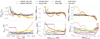 |
Fig. 4. Consistency of StarHorse input and output parameters. Top panels: median of the relative discrepancy between input parameters and StarHorse output parameters for each survey. Bottom panels: median of the dependence between input uncertainties versus input parameters. |
4.3. StarHorse MSTO-SGB ages and masses
For the first time, we publish ages derived with StarHorse. Ages (as well as masses) for individual stars are challenging to derive through isochrone fitting when only spectroscopic, astrometric, and photometric data are available (e.g. Joyce et al. 2023). In the absence of spectroscopic data, meaningful age estimates are even more complicated (Howes et al. 2019). More sophisticated methods such as asteroseismology or eclipsing binaries (where an additional constraint on the stellar mass becomes available) are much more reliable for deriving ages, and these methods can achieve uncertainties below 10% (Valle et al. 2015; Silva Aguirre et al. 2018; Anders et al. 2017; Valentini et al. 2019; Miglio et al. 2021). The downside is that the samples with asteroseismic and eclipsing binaries are still limited in size and pencil beams compared to spectroscopic surveys. We can achieve more statistical significance by measuring less precise ages but for larger sets. Here we do so, but we restrain ourselves to the MSTO-SGB. In these evolutionary stages, isochrone fitting methods are more reliable since the shape and duration of this stage varies strongly with the stellar mass and, therefore, the age. For SGB stars, the luminosity correlates directly with age, which makes this stage specially suitable for isochrone-based age determinations (e.g. Xiang & Rix 2022). In Q18 (e.g. Fig. 4) we also show with simulations that StarHorse ages can achieve relative statistical uncertainties of 20% for SGB stars.
Isochrone age determination can be highly uncertain and subject to biases in input temperature, surface gravity, or metallicity (see Queiroz et al. 2018). To mitigate these effects, we undertook a cleaning procedure of the input parameters of each spectroscopic survey. Specifically, for the MSTO-SGB ages, we applied the recommended flags from the spectroscopic pipelines and implemented a minimum signal-to-noise cut of 30 in all surveys. Table 3 provides the details of our cleaning procedure. The quality cuts are done using flags describing the quality of the spectral observations or the derivations of atmospherical parameters. These are described in more detail in the indicated papers and web pages. In our final catalogue, we have included a flag to indicate whether stars are at the MSTO or SGB stage, as well as a flag ‘age_inout’ to alert users of any significant differences between the input and output spectroscopic parameters (Teff, log g, met50).
Flags we clean for age computation in each survey.
We display our MSTO-SGB selection in Fig. 5. We opt to use the output StarHorseTeff and log g for this selection, since we saw in Sect. 4.2 that for some surveys there are systematic differences between input and output parameters (especially in Teff and log g). Therefore, a selection using the StarHorse parameters is more homogeneous and, to some extent, helps eliminate systematics between the different spectroscopic surveys. StarHorse can break degeneracies by accessing the extra information from photometry and astrometry. The selections are performed using the following equations adjusted by eye to comprise the MSTO and SGB regime:
 (1)
(1)
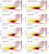 |
Fig. 5. StarHorse Kiel diagram for the samples studied in this work. The grey dots in the background of each panel show all the stars in the respective survey, while the colour-coded histograms highlight the MSTO+SGB regime for which we deliver StarHorse ages. The dashed lines delimit the SGB, for which the computed ages are most precise. PARSEC isochrones are overplotted in red for three different metallicities, as indicated in the lower-right corner of the figure. For each metallicity, four different ages are shown: 1, 4, 7, and 10 Gyr. |
And only for the SGB selection:
 (2)
(2)
In Fig. 6 we show the distributions and uncertainties in ages and masses for the selected MSTO-SGB stars. Most age distributions display two peaks: one at intermediate ages (≈3 Gyr) and one containing an older generation (≈9−11 Gyr). There is a noticeable depression at 10 Gyr for the higher-resolution surveys APOGEE, LAMOST MRS, and GALAH. Since the SDSS/SEGUE survey preferentially targeted the Galactic halo, the age distribution for this survey is highly skewed towards old ages, and presents a double peak at 11 and 12 Gyr. GES and LAMOST LRS only show a rise at 11 Gyr. 90% of the MSTO stars have relative age uncertainties smaller than 50%, and their average is below 34% (see Table 2). For SGB stars, this average decreases below 20%. From all the spectroscopic releases, APOGEE and LAMOST MRS have the smallest nominal uncertainties in age (below 10%), although this is strongly driven by the input parameter uncertainties of the surveys. We caution, therefore, about the systematic differences on the uncertainty of our derived ages from one survey to another. The spectroscopic surveys make very different choices on how to report uncertainties in their atmospheric parameters (some of them are probably underestimated in some surveys), which then will lead to underestimated age uncertainties.
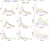 |
Fig. 6. Distributions of ages, masses, distances, and their uncertainties for the MSTO+SGB samples. The y-axis shows the probability density. All histograms are normalised so that the area under the histogram integrates to 1. The right panels show the mean age uncertainty per bin of age, mass, and distance for each survey. |
Apart from ages, we also deliver mass estimates for the complete catalogues, not only the MSTO-SGB, but we remind the user to be cautious when using these values, since both statistical and systematic uncertainties can be very high (depending on the class of stars). The posterior mass distributions do not show considerable differences between surveys, besides the higher content of low-mass stars in SDSS and GES. Our mass estimates have been previously validated in earlier StarHorse versions (Q18), against asteroseismic and binaries samples, which yielded relative deviations of ≈12% and 25%.
In Fig. 6 we also show the extent of heliocentric distances for the MSTO-SGB samples, which is mainly confined to an extended solar neighbourhood (0.1−3 kpc). Surveys targeting the halo, such as GES and SDSS, do reach farther distances even inside the MSTO-SGB selection. In the right panels of Fig. 6 we see the dependence of the relative age uncertainty with age, mass and distance. StarHorse ages are more uncertain for younger, intermediate-mass stars. There is also a trend of decreasing age uncertainty with distance, which is related to older stars being found far from the disk. This effect is evident in Fig. 7. For all surveys, we see dependence of age and Galactic height (Zgal) more explicitly in LAMOST LRS, which has the most significant number of stars. The increasing age with Zgal shows the consequence of transiting between the young, thin disk (confined to the Galactic plane) to the older thick disk and halo components.
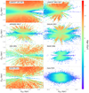 |
Fig. 7. Galactocentric X and Z projection of MSTO+SGB samples colour-coded by StarHorse ages. The colour bar is in power law scale with γ = 0.7. |
4.4. Validation of age estimates
Since age estimates for field stars are highly dependent on stellar evolutionary models, it is important to identify (and, when possible, quantify) systematic biases. Although also not model-independent, asteroseismic and OC ages are still our best anchor for validating field-star age estimates. Since solar-like oscillations in MSTO-SGB stars are much weaker than for the red-giant branch, large samples of MSTO-SGB benchmark ages from asteroseismology are still missing. In Fig. 8 we therefore compare our age estimates to the OC ages derived by Cantat-Gaudin et al. (2020). Almost all considered spectroscopic surveys have observed at least some OCs with MSTO-SGB members, For SDSS and RAVE there are fewer than five cluster members, which therefore we chose not to show. The results of the test shown in Fig. 8 are for the most part reassuring. While the results are on average in good agreement, specially for the SGB sample only, the ages of younger OC MSTO members present some systematically overestimated results. We verified that most of this disagreement is due to an input temperature, gravity, or metallicity that is not consistent with the ages determined by Cantat-Gaudin et al. (2020). There might be a systematic in the determination of atmospheric parameters for younger ages as well, and therefore we carefully cleaned the sample of potential problems in the spectral parameters derivation indicated by each survey in Table 3.
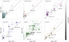 |
Fig. 8. Comparison of our MSTO+SGB age estimates with OC ages from Cantat-Gaudin et al. (2020). In each panel, grey dots are individual OC member MSTO stars (membership probability > 95%), colour-coded by their posterior age uncertainty. For OCs that contain more than three MSTO cluster members, the uniform coloured points and error bars indicate the median age and the 1σ quantiles. The star symbol indicates the SGB-only sample, which has lower StarHorse uncertainties. The horizontal error bars reflect the 0.2 dex uncertainties quoted by Cantat-Gaudin et al. (2020). The only OC that was observed by all surveys is M 67 (NGC 2682). We do not show comparisons for RAVE and SDSS since there were fewer than five stars in common with the cluster sample. The dashed black line delineates the identity line, while the grey dashed lines correspond to a ±30% deviation. |
Another reason for this is the dominance of the initial-mass function prior, which for massive stars will result in the preference of lower-mass (and consequently, older-age) posterior solutions. We insist, however, that this is not a genuine problem of the StarHorse code, but a generic problem of one-fits-all isochrone-fitting codes.
Proof of this statement (as well as a secondary sanity check) is provided in Fig. 9, which compares our age estimates to field-star ages in the recent literature (Xiang & Rix 2022; Buder et al. 2021; Leung & Bovy 2019; Mints 2020). The figure demonstrates that our age estimates compare well with other recent attempts to derive isochrone ages, especially with the ages derived by Buder et al. (2021) for GALAH DR3 and, to a slightly lesser degree, with the results obtained by Xiang & Rix (2022) for LAMOST and Mints (2020) for APOGEE, RAVE, and LAMOST. The horizontal streaks in the comparison figures for the Mints (2020) results (lower panels of Fig. 9) stem from the fact that they used a PARSEC grid with equal spacing in log age rather than linear age (as done in this StarHorse run). The significant scatter seen in each of the panels of Fig. 9 demonstrates that, even when similar techniques and the same input data are used, results vary systematically. To give an extreme example, some of the GALAH DR3 stars that StarHorse indicates to be young (< 500 Myr) are found to be old by Buder et al. (2021), which is very likely to be a combination of a grid-edge effect and poor stochastic sampling of the posterior.
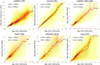 |
Fig. 9. Comparison of our MSTO+SGB age estimates with values from the recent literature. From top left to bottom right: comparison to the LAMOST DR7 ages of Xiang & Rix (2022), the GALAH DR3 ages of Buder et al. (2021), the LAMOST, RAVE, and APOGEE age estimates of Mints (2020), and the ages calculated by Kordopatis et al. (2023) for the Gaia RVS sample. In each panel we show the number density of stars, and the magenta points indicate the median trends. The global spread for each comparison is shown as the mean absolute deviation (mad) and the global shift as the mean deviation (mad). |
5. Age-abundance relations
The advantages of combining Gaia with spectroscopic data are not limited to more precise distances and stellar parameters, but also opens the possibility to study detailed chemical abundances as a function of these parameters. Certain abundance ratios are strongly correlated with age in our Galaxy and can indicate the formation of different populations (Chiappini et al. 1997; Tucci Maia et al. 2016; Miglio et al. 2021; Morel et al. 2021). These relations between age and chemistry are potentially of great value for understanding and constraining Galaxy evolutionary models (Chiappini et al. 2014; Nissen 2015; Miglio et al. 2017). In this section we investigate if we can recover some of the known age-chemical correlations between the StarHorse ages, metallicity, α-process and as s-process elements. This exercise also serves as an additional validation for the new StarHorse MSTO-SGB ages.
5.1. α abundances and metallicities
Since α elements are known to be produced mainly by the massive dying stars in type-II SNe, those elements had a larger relative contribution to the chemical evolution of the Milky Way in the past. On the other hand, the content of elements produced by type-Ia SNe increases slowly with the enrichment of the interstellar medium. Therefore, the ratio of α-capture content with iron can be broadly associated with the temporal evolution of stellar populations (Tinsley 1980; Matteucci & Francois 1989; Chiappini et al. 1997; Woosley et al. 2002).
Diagrams of [α/Fe] versus [Fe/H] have also been generally used as a classification of the stellar components of our Galaxy: the chemical thick disk is mostly at high-[α/Fe] sequence, while the thin disk can be chemically selected as the low-[α/Fe] sequence (Edvardsson et al. 1993; Fuhrmann 1998; Adibekyan et al. 2012). The morphological thin and thick disks do not coincide exactly with their chemical definitions, thick disks form from the nested flares of mono-age populations, as shown by Minchev et al. (2015). This model explained for the first time the presence of low-α stars high above the disk midplane in the outer Galaxy (Anders et al. 2014; Hayden et al. 2015) and the predicted strong negative age gradient the Milky Way morphological thick disk was indeed confirmed by Martig et al. (2016). The high-[α/Fe] sequence or chemically defined thick disk is mostly assumed to be old, while the low-[α/Fe] sequence is younger, but the position and shape of these sequences are known to vary across the Galaxy (Bensby et al. 2011; Anders et al. 2014). The inner disk, for example, shows a more prominent bimodality indicating different star formation paths and evolution across the Galaxy (Q20). The picture also gets more complex with the detection of young-α-rich stars (Chiappini et al. 2015). Therefore, we expect a clear correlation between [α/Fe] and age but also a large spread due to the mixing of populations (Anders et al. 2017, 2018; Miglio et al. 2021). In Figs. 10 and 11 we show that most of the old stars populate the high-[α/Fe] sequence, and we confirm a relation of increasing [α/Fe] for increasing StarHorse age for most spectroscopic surveys, but also a significant scatter (as expected). Older ages are also visible in Fig. 10, especially for the APOGEE and LAMOST surveys, at high metallicities and low-α linking the formation of the chemical thick disk and the inner thin disk in a knee where the [α/Fe] ratio decreases at a constant rate as a function of [Fe/H] when the type-Ia SN contribution becomes important. Another set of old stars is seen in almost all surveys at low metallicity and low [α/Fe], which is compatible with the chemical characteristics of dwarf Galaxies and the most outer parts of the Galactic thin disk. Although the age and α scatter is high in Fig. 11 for most surveys, one can notice that spread in age is considerably smaller for high-α populations, suggesting that the old high α sequence was formed in shorter timescale and as expected from chemo-dynamical models (Minchev et al. 2017). This result is also seen by Miglio et al. (2021), using precise asteroseismology from red giant stars with Kepler and APOGEE spectra, which showed that the old thick disk has a spread smaller than 1.2 Gyr.
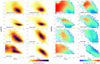 |
Fig. 10. [α/Fe] versus [Fe/H] distributions for the MSTO+SGB samples of the analysed surveys. Left: density distributions relative to the maximum count in each survey. Right: same, but coloured by the mean age per pixel. |
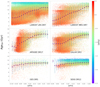 |
Fig. 11. [α/Fe] versus age distribution for the MSTO+SGB samples of each survey. A cleaning per signal to noise and suggested flags was performed. The purple squares show the median trend per bin in [α/Fe], while the error bars show its one σ deviation. We only display the surveys that have mean statistical uncertainty in age < 20% according to Table 2 (no RAVE or Gaia RVS). We also performed a cleaning of flags in the [α/Fe] determination from each survey. |
5.2. s-process abundances
The slow neutron-capture process (s-process) elements are produced in the asymptotic giant branch (AGB) phase of low- and intermediate-mass stars, and hence their contribution to the interstellar medium increases steadily with time (Busso et al. 1999; Sneden et al. 2008; Kobayashi et al. 2020). Studies of low-metallicity AGB stars also show a strong component of s-process elements in the Galactic halo (Sneden et al. 2008; Bisterzo et al. 2014). Among the spectroscopic surveys considered in this work, APOGEE and GALAH have measured precise high-resolution abundances for a few neutron-capture elements for a significant number of stars in the SGB regime. We chose these two surveys to explore the ratio between s-process (yttrium, barium, and cerium) and α elements with age.
In Fig. 12 the ratios between [Ba/α] and [Y/α] show a linear dependence with age. The data points in Fig. 12 are fitted with a non-linear least mean square method, and its uncertainty is taken as a square root from the covariance matrix. It is worth mentioning that the uncertainty associated with the fits done here are probably underestimated due to the large datasets and the noise it contains, which are not variables in the fitting procedure (Hogg & Villar 2021), but doing a full Bayesian fit is out of the scope of the paper. In the GALAH data, both [Ba/α] and [Y/α] show strong relations with age. The [Y/Mg] chemical clock has been extensively studied in other works, from solar twins to clusters (Spina et al. 2018; Maia et al. 2019; Nissen et al. 2020; Casamiquela et al. 2021a). This relation has no apparent variation with metallicity (Nissen et al. 2020). In Table 4, we compare our resulting relations for different chemical clocks with previous works. For [Y/Mg], the linear trend with age agrees very much well with Casamiquela et al. (2021a), which is a higher value compared to the other works but still close to the values found by Spina et al. (2018) and Jofré et al. (2020). For [Ba/Si] and [Ba/Mg], our results lay in between the different relations found in the literature, overall more in agreement with Jofré et al. (2020). This shows that StarHorse ages are, at least, meaningful in population studies and do reproduce expected chemical-clock relations. The differences between slopes found in the literature can be attributed to the different ranges in metallicity (Horta et al. 2022; Viscasillas Vazquez et al. 2022), the overabundance in neutron capture elements in OCs compared to dwarf field stars (Sales-Silva et al. 2022) or still the different spectroscopic pipelines. In Appendix A we show figures identical to Figs. 12 and 13 except colour-coded by temperature and metallicity. In Fig. 13 we show yet another s-process element, Cerium, derived by the ASPCAP Synspec pipeline (Jönsson et al. 2020). The precision for Cerium in APOGEE is much lower than the previously discussed s-process abundances in GALAH. It is noticeable from the figure that there is a high spread in [Ce/α] versus age and that most of the cerium abundances are below the solar value. In fact, a considerable shift between the Cerium derived by APOGEE and other surveys has been reported for giant stars in the Galactic bulge (Razera et al. 2022) and when compared to Gaia DR3 RVS spectra (Contursi et al. 2023). In a recent work, Sales-Silva et al. (2022) show, also using APOGEE, that [Ce/α] has a strong dependence on metallicity and does not work as a universal chemical clock. In light of these complexities, the relations between [Ce/α] abundances and age derived in this work are almost flat and have lower values than other studies in the literature (Jofré et al. 2020).
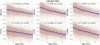 |
Fig. 12. [s/α] abundance ratios versus age for GALAH. The purple line shows the median abundance per age bin, and the error bar represents a one sigma deviation from the median. |
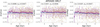 |
Fig. 13. [s/α] abundance ratios versus age for APOGEE. The purple line shows the median abundance per age bin, and the error bar represents a one sigma deviation from the median. |
6. Analysing chemo-age groups of local SGB samples
As an example science case for our new catalogues, we chose three spectroscopic surveys (GALAH DR3, APOGEE DR17, and LAMOST MRS DR7) to map different populations with high or medium-resolution spectroscopic abundances in the local sample of SGB stars. We chose to only use the SGB since it is a fast evolutionary stage where ages have an explicit dependence on its luminosity, resulting in lower StarHorse uncertainties (see Table 2). We see in Sect. 4.4 that there is a better agreement for OCs in the case of SGB. In Sect. 5 there is a clear relation between [Ba/α], [Y/α], and age for these stars, which all substantiate the robustness of the StarHorse derived ages for the SGB regime. The three surveys were chosen due to their higher-quality abundances and completeness. In this section we use the dimensionality reduction visualisation t-SNE technique (Hinton & Roweis 2003; van der Maaten & Hinton 2008), in synergy with HDBSCAN (Campello et al. 2013; McInnes et al. 2017). In the following subsections we describe t-SNE and HDBSCAN as well as their application to the SGB samples.
6.1. Methodology: t-SNE and HDBSCAN
Finding groups of chemically similar stars aids our understanding of the formation and evolution of the Milky Way (Freeman & Bland-Hawthorn 2002). Stellar chemical abundances of most elements remain constant during most of stellar evolution, while a star’s orbit can be changed radically depending on the gravitational perturbation it suffers. The composition of a star’s birth cloud dictates its chemical composition, making it possible to identify stars born in similar conditions through weak chemical tagging (e.g. Hogg et al. 2016). However, differences in chemical abundances can be very subtle and become masked by their observational uncertainties making strong chemical tagging or finding co-natal stars very difficult (Casamiquela et al. 2021b). It is also important to take into account the radial migration due to the dynamical effects produce by the non-axisymmetric structures (bar and spiral arms).
One way to explore this problem is by visualising the entire complex multi-dimensional chemical abundance and age space at once to find patterns in an easier manner. t-SNE is a statistical method for visualising high-dimensional data by giving each data point a location in a two or three-dimensional map (van der Maaten & Hinton 2008). These maps are iteratively created by minimising the Kullback-Leibler divergence between the similarity distributions of the data in the original space and the low-dimensional map, and thus preserve the proximity between similar data points. For a slightly deeper introduction focussed on a similar science case, we refer to Sect. 2 in Anders et al. (2018). As in that paper, we use the python implementation of t-SNE included in scikit-learn (Pedregosa et al. 2011).
The t-SNE technique is an effective tool to help identify peculiar groups in different parameter spaces and has wide applications in astronomy, for example stellar spectral classification (Matijevič et al. 2017; Traven et al. 2017; Valentini et al. 2017; Verma et al. 2021; Hughes et al. 2022), similarities between planetary systems (Alibert 2019), and galaxy classification (Zhang et al. 2020; Rim et al. 2022). Finally, Anders et al. (2018), Kos et al. (2018), and Nepal et al. (in prep.) show that applying t-SNE to the abundance space to perform chemical tagging confirms cluster, stream membership and different stellar populations that compose the Galactic disk. Inspired by those works, we follow a similar approach but with a few differences; we apply t-SNE to a set of chemical abundances combined with the age information of APOGEE, GALAH, and LAMOST MRS and then, instead of looking for separations in the t-SNE by eye, we apply a clustering method to identify different chemical-age groups.
Clustering algorithms have been extensively used in astronomy to find stellar groups in the kinematical or chemodynamical space (Koppelman et al. 2019; Limberg et al. 2021; Gudin et al. 2021; Hunt & Reffert 2021; Shank et al. 2022). For example, HDBSCAN is an extension of the DBSCAN (Ester et al. 1996) clustering method. It converts DBSCAN into a hierarchical method by extracting flat clustering based on the stability of the clusters, which leads to the detection of high-density clusters, and it is, therefore, less prone to noise clustering than DBSCAN.
The configuration of t-SNE+ HDBSCAN for each of the samples we discuss in the following sections is displayed in Table 5. The main hyperparameter of t-SNE is called perplexity and controls the number of nearest neighbours. We made several tests with different values for the perplexity parameter and the random state, which can influence the local minima of the cost function (Wattenberg et al. 2016). These tests are summarised in Appendix C. We always chose the t-SNE configuration that visually splits the groups more clearly.
Configuration and input parameters of t-SNE+HDBSCAN.
We applied HDBSCAN to the t-SNE projections. The three relevant hyperparameters described in Table 5 were optimised to obtain the ‘best’ clustering in the sense of weak chemical tagging, that is, a configuration that does not split the data into too many small groups. Since we are searching for a more global picture of the chemistry and age distribution of stellar populations, we know that a large group should be found by the method as the ‘thin disk’ since it should dominates our samples. The HDBSCAN hyperparameter ‘min_cluster_size’ controls the minimum number of stars allowed to be considered a cluster; this parameter depends on the sample size (see e.g. McInnes et al. 2017, and our Appendix C). The hyperparameter ‘min_samples’ defines how conservatively the method treats noisy data. Finally, the hyperparameter ‘cluster_selection_epsilon’ controls the distance between the clusters, which can change with the t-SNE projection. We also always set HDBSCAN to ‘eom’ as the cluster_selection_method, which is optimised for larger groupings.
6.2. SGB samples
In this subsection we detail the exact selection of the elemental abundances and ages used for the following t-SNE and HDBSCAN analysis, separately for the APOGEE, GALAH, and LAMOST MRS samples. While this is important to understand the differences in the results for the three surveys, readers mainly interested in the overall results may consider to move on straight to Sect. 6.3 in which we discuss the chrono-chemical groups found in our analysis.
6.2.1. APOGEE DR17
We used APOGEE DR17 abundances from the SGB sample to find groups in the t-SNE projection with HDBSCAN. We applied the following quality cuts before executing t-SNE: SNREV > 70, ASPCAP_CHI2 < 25, VSCATTER < 1, ASPCAPFLAG = 0, STARFLAG = 0, ‘NEGATIVE’ not in StarHorse_OUTPUTFLAGS, and ‘CLUSTER’, ‘SERENDIPITOUS’, and ‘TELLURIC’ not in TARGFLAGS. And finally, we also made a strict cut in temperature 5500 K < Teff < 6000 K.
In Table 5, we list the abundance ratios chosen as input for the t-SNE method, we only select elements with a relatively small uncertainty, as seen in Fig. B.1. In the abundance group, we have iron-peak, odd-Z, and α elements. The s-process element cerium is not included because of the large uncertainties and poor statistics for the SGB sample. We need to be cautious when using APOGEE abundances since its pipeline is optimised for giants (Jönsson et al. 2020). In the case of subgiants, there might still be many artefacts (e.g. Souto et al. 2021, 2022; Sales-Silva et al. 2022) that could possibly lead t-SNE and HDBSCAN to find an unphysical clustering in the chemo-age space. In Fig. B.1 we see some drastic differences when one uses different spectral analysis codes in the APOGEE pipeline. Even for abundances with minimal errors like [Al/Fe] and [Si/Fe], there is a significant difference at temperatures below Teff < 5500 K, thus our strict temperature cut. After a further cleaning per each abundance flag, elem_flag = 0, we are left with 4638 stars to which we apply t-SNE and HDBSCAN.
In the case of APOGEE, the method finds at least three different groups (see Fig. 14 and tests with t-SNE parameters in Fig. C.3). To check if there is any dependence of the t-SNE clustering with the abundance pipeline, we also show in Fig. C.4, which displays the final t-SNE projections colour-coded by Teff, log g, [Fe/H] and signal-to-noise ratio. Some areas of the resulting projections are predominantly found at a metallicity and Teff range. This indicates that the clustered groups have a certain dependence on those parameters. The groups differ in [α/Fe] content, metallicity, and also in their age distribution. While most of the stars belong to a (chemically defined) ‘thin-disk’ component ≈ with high dispersion in metallicity and age, two other groups are found with chemical characteristics of ‘thick disk’ and ‘transition’ or ‘high-α metal-rich’ stars (Fuhrmann 2008; Adibekyan et al. 2011; Anders et al. 2018; Ciucă et al. 2021). We discuss these groups in more detail together with the ones found in GALAH and LAMOST in Sect. 6.3 and in Appendix C.
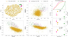 |
Fig. 14. General results of the t-SNE+HDBSCAN application. Upper-left panel: t-SNE projection for SGB stars in APOGEE DR17. Colours correspond to different groups found by t-SNE+HDBSCAN on the data. Lower-left and middle panels: abundance ratios of α elements to those of the iron group plotted against metallicity using the same colours for each identified group. Right panels (from top to bottom: i): (i) cumulative age distribution for each group; (ii) mean azimuthal velocity (left y-axis and square symbol) and mean dispersion in azimuthal velocity (right y-axis and star symbol) for each group as a function of age; (iii) mean vertical velocity (left y-axis and square symbol) and mean dispersion in vertical velocity (right y-axis and star symbol) for each group as a function of age; (iv) mean metallicity (left y-axis and square symbol) and mean dispersion in metallicity (right y-axis and star symbol) for each group as a function of age. The error bars in the right panels represent the 95% confidence interval of a bootstrap resampling. |
6.2.2. GALAH DR3
Similarly to APOGEE, we use GALAH DR3 abundances for the SGB sample to find groups in the t-SNE projection with HDBSCAN. Before performing the analysis, we made the quality cuts suggested by Buder et al. (2021): snr_c3_iraf < 30, flag_sp = 0, flag_fe_h = 0 and ‘other’ not in survey_name, as well as anything with negative extinctions in StarHorse. The chemical abundances that we chose for the analysis are described in Table 5. The set contains iron peak elements as well as α and neutron capture elements, covering different nucleosynthetic paths. From this group of abundances, we select only stars for which the flag_elem = 0. The GALAH DR3 SGB sample that satisfy all the mentioned flag conditions is reduced from 47 524 to 9420 stars. We did not choose all abundances available in GALAH since this reduces the sample size even more drastically. We then combine the chosen abundance ratios from Table 5 together with the ages from StarHorse as t-SNE input. Here we also experiment with the different test parameters on t-SNE seen in Fig. C.1. For the GALAH sample we select the case for perplexity = 100 and random state = 30. To check if there is any dependence of the t-SNE clustering with the abundance pipeline, we also show in Fig. C.2 the final projections colour-coded by Teff, log g, [Fe/H] and Signal to noise, again here as expected there are some dependences in temperature and therefore metallicity.
We then apply HDBSCAN to the t-SNE projection, with the parameters described in Table 5. The results from the t-SNE projection and HDBSCAN clustering groups are shown in Fig. 15 along with various abundance relations for the different coloured groups. We discuss a possible interpretation for each of the groups in Sect. 6.3, with a particular focus on the chemical thick disk.
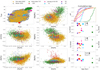 |
Fig. 15. t-SNE projection for SGB stars in GALAH DR3. Colours correspond to each group found by t-SNE+HDBSCAN from GALAH data. Abundance ratios are also shown, with the same colour coding. Upper panels: cumulative age distribution for each group. Middle panels: mean azimuthal velocity (left axis squares) and mean dispersion in azimuthal velocity (right axis stars) for each group. Lower panels: mean vertical velocity (left axis squares) and mean dispersion in vertical velocity (right axis stars) for each group. The error bars in the right panels represent the 95% confidence interval of a bootstrap resampling. |
6.2.3. LAMOST MRS
As a final exploration of the t-SNE+HDBSCAN method, we chose the medium-resolution survey from LAMOST. It is essential to keep in mind that this has a lower resolution than the previously discussed surveys APOGEE and GALAH. LAMOST MRS has 12 individual element abundances, derived through a label-transfer method based on a CNN using as training set APOGEE spectra (Xiang et al. 2019). There are many caveats in such methodologies, for example the incompleteness and noise in the training data and the unavailability of uncertainties. Therefore, we must be aware of these problems when analysing the results. To proceed with the method, we made the following quality cuts to LAMOST MRS SGB sample: S/N > 30, fibermask = 0 and 3500 < Teff < 6500. We decide on the chemical abundances from LAMOST shown in Table 5. The choice is mostly based on the mutual availability of the abundances since we do not have uncertainties or flags to control in this sample. With these choices we are left with 12 834 stars in LAMOST DR7 SGB sample. Combining the set of abundances with ages into the multi-dimensional space t-SNE+HDBSCAN can find three different groups as seen in Fig. 16 together with some abundance ratios, age and kinematical properties. We discuss a possible interpretation in the next subsections.
6.3. Chrono-chemical groups
In this subsection we describe the physical properties of the groups discovered in APOGEE, GALAH, and LAMOST surveys with the t-SNE+HDBSCAN method. Given the difficulty of accurately determining the uncertainties associated with each group association, we place greater emphasis on those groups that were identified in all three surveys, namely the genuine thick disk, thin disk, and young α-rich groups. In Fig. 17 we present the average distribution of their properties (metallicity, age, and α-enhancement). It is worth noting that due to the significant differences in the quality of the stellar parameters and sample selection of each survey, the distributions of the same populations can present some differences in their properties, such as extended tails and number of peaks.
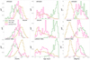 |
Fig. 17. Probability density function of metallicity, age, and [Mg/Fe] for the main populations found in APOGEE, GALAH, and LAMOST with t-SNE HDBSCAN. |
6.3.1. Thin disk stars (dark yellow)
Traditionally, the disk in the Milky Way and in external galaxies (Dalcanton & Bernstein 2002) can be divided into geometric thin and thick disks. The thin disk dominates in density in the solar neighbourhood since its geometrical component is denser and mostly confined to the Galactic plane. In contrast, the thick disk has a more extensive scale height (Jurić et al. 2008). Since our selection of SGB stars are limited to the solar neighbourhood, we expect that our samples have a strong dominance of thin-disk-like stellar populations. However, the disks defined chemically and geometrically are not identical (see Kawata & Chiappini 2016; Minchev et al. 2015; Anders et al. 2018 for a discussion). Our method for recovering chrono-chemical groups finds mostly stars similar to a chemical thin-disk highlighted with the dark yellow colour in Figs. 14–16. Chemically, the thin disk is much more complex and less well mixed than the chemically defined thick disk. A metallicity gradient with radius has been long reported as a characteristic of the thin-disk (Anders et al. 2014; Hayden et al. 2015) and radial migration is efficient in circular orbits, which can bring stars born in a certain inner radius to the solar neighbourhood (Minchev et al. 2011, 2013). With all these complexities, we expect that a technique to search chrono-chemical groups could find multiple systems in the thin disk. Our results show that the thin-disk population has a broad age and metallicity distribution, and multiple systems are found in the GALAH DR3 sample. The chemical composition of the thin disk does not extend much beyond 0.1 dex in α-abundances, and their enrichment in s-process elements is higher than the detected thick disk (green dots), but there is also considerable overlap. The thin disk has orderly rotation, with smaller velocity dispersion and high rotational velocities, as seen in the right panels of Figs. 14–16. All those characteristics are consistent with the chemical and kinematical thin disk populations defined in multiple works in the literature (e.g. Adibekyan et al. 2013; Anders et al. 2018). The mean age of the thin disk detected in this work lies between 5 and 6 Gyr, depending on the survey. We notice from Fig. 17 that the thin disk age distributions have slight differences from survey to survey; all surveys show a prominent peak at about 3 Gyr, with GALAH having a higher proportion of those young stars. While in GALAH, the thin disk stars steadily decrease in proportion with age, APOGEE shows a secondary peak at 6 Gyr, and LAMOST mainly presents a flat distribution from four to eight Gyr. Curiously on APOGEE and LAMOST, the thin-disk extends to ages larger than ten Gyr; these stars are older than one would expect for standard thin-disk formation scenarios, even though recently Prudil et al. (2020) also found evidence for a population of RR Lyrae stars older than 10 Gyr with chemo-kinematical thin disk characteristics. We can attribute the differences in the thin disk’s age distribution between surveys to their different selection functions or to the breakage into subpopulations; another issue is the different solar scales utilised in the surveys, which can lead to differences in the chemical distributions. Furthermore, the consistent result of a broad age distribution throughout the surveys is in line with a slow and inside out formation of the chemical thin-disk component (e.g. Chiappini et al. 1997, 2001; Minchev et al. 2013, 2014). In Fig. 18 we show the thin disk’s age versus metallicity in the three surveys. We see that for the thin disk populations, there is a clear relation of increasing ages to decreasing metallicities until about 3 Gyr, which corresponds to the prominent young peak seen in the age distributions of Fig. 17. After 3 Gyr, the relation between age and metallicity becomes more complex. Still, there is an apparent change in the relation, suggesting an overall flat relation in age with metallicity but with high dispersion. As other works have shown it is complicated to reach strong conclusions from currently available age–metallicity relations, still affected by substantial age errors and important and difficult to correct selection effects (Feltzing et al. 2001; Casagrande et al. 2011; Bergemann et al. 2014). Even though we can separate the thin disk via the chrono-age groups, we need to correct for selection effects, which is out of the scope of this paper. We refer to future works for a proper analysis of the age metallicity relation of these samples.
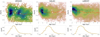 |
Fig. 18. Age metallicity relations for the thin disk. Upper panels: metallicity versus age for the detected thin-disk component in three surveys. The map shows the mean density per pixel where we have also applied Gaussian smoothing. The dotted red line represents the median metallicity for the given age. Lower panels: heliocentric distance coverage for each sample. |
6.3.2. Genuine thick disk stars (green)
We find stars compatible with the abundance pattern of chemically defined thick disk stars (Reddy et al. 2006; Adibekyan et al. 2011; Bensby et al. 2014; Anders et al. 2014; Nidever et al. 2014; Mikolaitis et al. 2014; Hayden et al. 2015), which present high alpha abundances in the three different SGB samples for which we run t-SNE+HDBSCAN. Here we refer to this population as the ‘genuine thick disk’. These stars clearly occupy the high-[Mg/Fe] sequence in the classical Tinsley-Wallerstein diagram (Wallerstein 1962) (lower-left panel of Figs. 14 and 16 and the central panel of Fig. 15) and show elevated [Mg/Mn] and [Al/Fe] abundances (Das et al. 2020). In the GALAH sample, where we have the s-process abundance ratios such as [Ba/Fe], it shows a slightly lower location than the bulk of the populations. At the same time, [Zn/Fe] is mildly enhanced compared to the thin disk at the same metallicity in agreement with previous measurements (Delgado Mena et al. 2017; Friaça & Barbuy 2017). In the right panels of Figs. 14–16 we show the cumulative age distribution as well as the age–VΦ, age–σVΦ, age–VZ, age–σVZ relations, binned by HDBSCAN population. These plots show that the genuine thick disk is relatively old (≳10.9 Gyr), has lower rotation and is kinematically hotter than the thin disk populations, in line with the recent analysis of Rendle et al. (2019) and Miglio et al. (2021). This result also agrees with observations of disk galaxies at redshifts ≈2, Übler et al. (2019) measured velocity dispersions of about 45 km s−1 for thick disks observed at that look-back time. Is also very clear that the genuine thick disk found by t-SNE+HDBSCAN has a contrasting mean age difference and a noticeable jump in velocity dispersion compared with all the other populations in the SGB samples, suggesting that it has indeed a very different formation path in agreement with Chiappini et al. (1997, 2001), Reddy et al. (2006), Miglio et al. (2021). Recent self-consistent dynamical models of the Milky Way, also show distinctive characteristics in the kinematics and composition of the thin and thick disks (Robin et al. 2022). The age distribution of genuine thick disk stars in Fig. 17 shows a double peak. The second prominent peak at ages between 9 and 10 Gyr (very clear in the GALAH sample) is possibly the contribution of transition or bridge stars, previously detected by other works (Anders et al. 2018; Ciucă et al. 2021). The transition stars were probably formed in the inner Galaxy and extend from the high α abundances to low α and high metallicities, filling the gap between the thin and thick disks [α/Fe] diagram. Further analysis of bridge stars with t-SNE+HDBSCAN is a matter for a forthcoming paper (Nepal et al., in prep.). The metallicity distribution shown in the left panels of Fig. 17 is reasonably similar for the three samples of SGB stars, ranging from −1.5 to 0.0 and with a clear peak at around −0.5 dex. For APOGEE and LAMOST the metallicity distribution shows a second prominent peak at −0.8 dex. The [Mg/Fe] distribution is also analogous throughout the different surveys showing a smooth distribution from 0.1 to 0.4 dex. In Table 6 we compare the mean age, azimuthal velocity and their dispersion values. We see that the age values agree very well between the surveys, varying from 10.4 to 10.9 Gyr, and the highest age dispersion being that of LAMOST DR7, of 1.35 Gyr. The age and age dispersion might be higher for LAMOST and APOGEE due to minor debris contamination as we see some stars in the green group to extend to the very metal-poor side.
Mean parameters of the genuine thick disk found in the different surveys.
6.3.3. Young α-rich (magenta)
Although young α-enhanced stars cannot be explained by standard chemical evolution models, a significant number of them have been previously detected by diverse works in the literature (Chiappini et al. 2015; Martig et al. 2015; Jofré et al. 2016; Silva Aguirre et al. 2018; Ciucă et al. 2021; Miglio et al. 2021). Our method also recovers stars with such characteristics in the SGB samples of GALAH, APOGEE, and LAMOST, which we indicate by the magenta colour in Figs. 14–17. In Fig. 19 we show that most of the stars detected as the magenta group fall in the area delimited by the black curves. It is hard to explain with chemo-evolutionary models of the Milky Way stars that fall in this area (Chiappini et al. 2015). The young α-rich populations detected here show a mean age of about 5 Gyr for the three different surveys. The cumulative age distributions have truncation at about 7 Gyr, but we see an extension to older ages in GALAH and LAMOST. Those older stars could perhaps again be part of the transition or bridge stars that have intermediate chemical characteristics between thin and thick disks (Anders et al. 2018). The range of abundances of the young-α-rich stars is similar to the genuine thick disk (green dots), except that their metallicity and [α/Fe] distribution is more concentrated at intermediate values between thin-disk (dark yellow) and genuine thick disk stars (see Fig. 17). For LAMOST the metallicity distribution of the magenta stars is overall poorer than in APOGEE and GALAH, although their [Mg/Fe] is lower, which could classify some of those stars as debris (Hasselquist et al. 2021; Limberg et al. 2022b), outer disk, or a pipeline problem. Is worth mentioning that the [Mg/Fe] measure through CNN algorithm in LAMOST DR7 MRS is not always consistent with the [α/Fe] measured from the LASP pipeline (Wu et al. 2014). We also notice differences between the green and magenta stars in the [Mg/Mn] versus [Al/Fe] diagram: contradictorily in APOGEE these stars are richer in [Al/Fe], ranging from 0.2 to 0.5 dex, while in GALAH they range in [Al/Fe] from 0 to 0.2 dex. The kinematics of the young-α-rich stars is mostly hot from the right panels of Figs. 14–16 the magenta groups show velocities dispersion both vertically and azimuthally of about 35 km s−1. Although their mean Vϕ is similar to the one of the thin disk, the hot kinematics agrees with previous works (Silva Aguirre et al. 2018; Miglio et al. 2021; Ciucă et al. 2021) suggesting that these stars formed from the same gas as the genuine thick disk but they appear young because they are probably mergers from binary stars (Jofré et al. 2016).
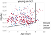 |
Fig. 19. Age versus [Mg/Fe] for the young α-rich groups found in APOGEE, GALAH, and LAMOST. The black delineation shows the region that chemical evolutionary models cannot explain, as in Chiappini et al. (2014). |
6.3.4. Other populations found in GALAH DR3
Enriched s-process stars (red). For the GALAH SGB sample, we can identify enhanced s-process stars since [Ba/Fe] is available and input to t-SNE. This chrono-chemical group shares very similar properties to the thin disk, showing low-α enhancement and a large dispersion in age and iron-peak elements, but a significant difference in barium enhancement, [Ba/Fe] > 0.5. The right panels of Fig. 15 show that these stars are slightly younger than the thin disk group, with a mean age of about 4.5 Gyr. Their rotation is similar to the thin disk, showing high azimuthal velocities and low-velocity dispersion. Despite the broad distribution in [Fe/H], these stars almost do not present any higher metallicities than Solar, and the most barium-enhanced stars are on the metal-poor side. One can also notice a considerable fall of [Ba/Fe] for metal-rich in the thin-disk (Israelian et al. 2014; Bensby et al. 2014). However, it could be challenging to measure barium at higher metallicities as mentioned before in Delgado Mena et al. (2017) and Buder et al. (2019). We also checked that the high [Ba/Fe] stars are also enriched in [Y/Fe] and [Zr/Fe]. The stars detected here do not belong to the enhanced barium stars seen as Am/Fm stars (Fossati et al. 2007; Xiang et al. 2020; Buder et al. 2021), since those are much younger, with high temperatures, Teff > 6500 K and extremely low α abundances. These enriched s-process stars could be the outcome of binary stars systems that have accreted mass from a dim white dwarf companion enriching them with heavy elements (McClure 1983). Two of the 103 stars detected here are also in the binary catalogue from Traven et al. (2020). Another possibility is that these stars come from an accreted dwarf galaxy, since in those systems stars can present a different chemical evolution than in the Milky Way.
Outer thin disk (cyan). The stars marked as cyan are mainly concentrated at the metal-poor end of the chemical thin disk, occupying the locus of outer disk stars in an [alpha/Fe] and [Fe/H] plot (Hayden et al. 2015; Queiroz et al. 2020). The different populations overlap in [Zn/Fe] and [Ni/Fe]. The cyan points show systematically larger [Ba/Fe] ratios than the thick disk stars (green), but also lower than the rest of thin disk stars. This is in a slight contradiction with the inside-out picture formation (Chiappini et al. 2001) in which the outer disk star formation history proceeds on longer timescales than in the inner parts of the Galaxy, leading to a larger Ba enrichment by low- and intermediate-mass stars. Perhaps this population is related to recent works finding metal-poor stars with thin disk rotation (Fernández-Alvar et al. 2021). We see from the right panels of Fig. 15 that the cyan population presents a steep age distribution at about 6.0 Gyr and has an older mean age than the thin disk. The [Mg/Mn] versus [Al/Fe] diagram, upper panel second column of Fig. 15, shows that the cyan population is at low [Al/Fe] and intermediate [Mg/Mn] borderline to the region occupied by dwarf galaxies (e.g. Limberg et al. 2022b; Hawkins et al. 2015; Das et al. 2020). The chemical characteristics and the older age attributed to this group could also indicate that these stars were formed by gas polluted by the accretion of a dwarf Galaxy, for example the Gaia-Enceladus dwarf, similar to what Myeong et al. (2022) recently suggested as a population named Eos, which would chemically evolve to resemble the outer thin disk. Another possible interpretation for the characteristics of the cyan group is that they are the outcome of the perturbation caused by one of the passages of the Sagittarius Dwarf. In the star formation history reconstructed by Ruiz-Lara et al. (2020), there is a clear peak at about 5.7 Gyr that coincides with the mean age of the cyan group found by the t-SNE+HDBSCAN method. The robustness of this group is not very strong when we introduce noise to the t-SNE method as seen in Appendix C, which means that this population has a weak signal in the data and needs further investigation. The tests with the random_state parameter in Appendix C also show that this group is not robust. Although it presents an interesting peaked age distribution, this grouping might be an artificiality introduced by the t-SNE+HDBSCAN method uncertainties.
Young chemically peculiar stars (navy blue, purple). These two groups of stars are amongst the youngest stars detected by our method. They present high rotational velocities and very low dispersion indicating these stars were probably formed within the thin disk. The navy-coloured stars show high [Ni/Fe] and low [Zn/Fe] content and are also at hotter temperatures, Teff > 6100 K (see Fig. C.2). The metallicity of the navy stars is concentrated in the metal-poor end of the thin disk, not extending further than Solar metallicities, similar to the previously discussed outer disk but significantly younger. The contribution of nickel is higher than iron in type-Ia SNe (Tsujimoto et al. 1995; Sneden et al. 1991). As we see in the left lower panel of Fig. 15 thin disk stars gradually become more [Ni/Fe] enriched for higher metallicities where SNe type Ia contribution dominates the interstellar medium. Therefore, it is puzzling that the stars rich in [Ni/Fe] have metallicities lower than solar. Since these stars are at a similar temperature range, it could also indicate a problem in the pipeline. In contrast, the purple stars cover almost the whole range of metallicities as the thin disk, but they present low [Ba/Fe], similar to thick disk stars and very low [Zn/Fe]. Trends of low [Zn/Fe] for higher metallicities are seen in the direction of the Galactic bulge (Barbuy et al. 2015; Duffau et al. 2017), although the stars that we discuss here appear too young to have migrated from the Galactic centre. It is also true that for these populations the robustness of the groups is heavily perturbed when we introduce noise to the t-SNE, as seen in Appendix C.
7. Conclusions
We present new StarHorse catalogues for eight (past and ongoing) spectroscopic surveys, coupled with Gaia DR3 and multi-wavelength photometry. We deliver a total of 10 998 676 distances, extinctions, masses, temperatures, surface gravity values, and metallicities, as well as ≈2.5 million age estimates for MSTO+SGB stars. For APOGEE DR17, results (except for ages) are also available as a VAC of the survey (Abdurro’uf et al. 2022).
Compared to the Q20 StarHorse release, we have included new results for more than 4 million stars from Gaia RVS spectra and additional data from LAMOST, GALAH, APOGEE, and GES. For RAVE DR6 and SDSS/SEGUE, we have updated our results to include Gaia DR3 parallaxes. We also made StarHorse ages available for the first time, selecting stars in the MSTO+SGB evolutionary stages since the age determination via isochrone fitting methods is not reliable outside of this regime.
Validation against other methods (Xiang & Rix 2022; Buder et al. 2022; Mints 2020) and OCs (Cantat-Gaudin et al. 2020) shows that our ages are trustworthy for stars older than 2 Gyr. StarHorse parameters have also been extensively validated in S16, Q18, and Q20.
We deliver typical distance uncertainties of about 4−10% and SGB age uncertainties of about 8−20%, depending on the survey’s spectroscopic resolution. For distances, our results are about 5 to 10% better than when spectroscopic information is not used (Anders et al. 2022; Bailer-Jones et al. 2021). The inclusion of Gaia DR3 astrometry, along with improvements in the spectroscopic pipelines of GALAH, APOGEE, LAMOST, and GES, allowed us to determine more precise parameters than in our earlier papers (Q18; Q20).
By combining the chemical abundances and radial velocities from spectroscopic releases with the final StarHorse data products, we were able to make the following findings:
-
We have shown classical diagrams of [α/Fe] versus [Fe/H] colour-coded by age for each of the eight spectroscopic surveys. The results manifest the old thick disk population at high [α/Fe], the old accreted metal-poor stars with low α abundances, and a transition population extending from the thick disk to the high metallicity inner thin disk stars with intermediate ages (Anders et al. 2018; Ciucă et al. 2021; Nepal et al., in prep.). We see a non-linear relation between α abundances and age for surveys with typical uncertainties below 30%. We also notice in Fig. 11 that the age dispersion decreases with increasing [α/Fe] in LAMOST LRS and that the age dispersion is about 3 Gyr for an [α/Fe] = −0.1 and only 1.4 Gyr for an [α/Fe] ∼ 0.3. The statistics are similar for the other surveys, indicating that old stars (mostly thick disk high-α stars) had a fast formation history (Miglio et al. 2021).
-
The dependence of s-process/α-process abundance ratios against age (chemical clocks) for the local sample of SGB stars reveals a linear correlation in most cases. The correspondence is strong for several abundance ratios, especially for [Ba/α]. A comparison with the results of Spina et al. (2018), Jofré et al. (2020), and Casamiquela et al. (2021a) for the same chemical clocks shows a similar effect, demonstrating that the StarHorse ages are sensitive enough to the abundance variations. The chemical clock’s determination also covers a large number of stars in the local volume of GALAH DR3 (≈18 000 stars).
-
Using an unsupervised machine learning approach coupled with a clustering algorithm, we can map different populations by their unique chemical age properties. For this exercise, we collected a set of abundances that span distinct nucleosynthetic paths and the SGB ages for three different surveys: APOGEE DR17, GALAH DR3, and LAMOST MRS. In all samples, we recovered the same three populations: chemical thin disk, genuine thick disk, and young α-rich stars, corroborating the method’s robustness. We stress that our method avoids pre-assumptions on the chemistry or kinematics of the thick and thin disk components of the Milky Way.
-
Our results show that the stars we obtained via the t-SNE+HDBSCAN cluster method and that follow the chemical pattern of the thin disk have low α abundances, a mean age of about 5.0 Gyr, prominent peaks at 3 Gyr, a flattened distribution from 4 to 9 Gyr, and span a broad distribution in metallicity. These chemical characteristics and the flattened distribution of ages are in line with the slow and inside-out formation of the thin disk (Chiappini et al. 1997; Minchev et al. 2013). At the same time, the younger counterpart shows the influence of mergers in the star formation history of the thin disk (Ruiz-Lara et al. 2020). In APOGEE and LAMOST, a small portion of stars also extends to ages greater than 10 Gyr, indicating clumpy star formation scenarios in the early disk (Beraldo e Silva et al. 2021).
-
Stars marked as green in Figs. 14–16 represent genuine thick disk stars. They have high [α/Fe] and lower metallicity, as seen by many works in the literature (Adibekyan et al. 2011; Bensby et al. 2014; Anders et al. 2014). We find mean age values in this group ranging from 10.38−11.77 Gyr depending on the survey, although all age distributions exhibit a double peak at ≈11.5 Gyr and ≈9.5 Gyr. The younger counterpart of the genuine thick disk is probably a contribution of another population described in the literature as transition or bridge stars (Anders et al. 2014; Ciucă et al. 2021). Further analysis of transition stars with high-resolution samples is part of a forthcoming paper (Nepal et al., in prep.). These results corroborate a formation scenario for the thick disk that happened at lookback times of z ≈ 2 (lookback time of 10−12 Gyr). According to this scenario, the small age dispersion of 1.05−1.35 Gyr indicates that the thick disk was fully formed before the interaction with Gaia Enceladus (Miglio et al. 2021; Montalbán et al. 2021).
-
The genuine thick disk dispersion in velocity is strikingly different from that of the thin disk, with values of standard deviation in vertical and azimuthal velocity of about 50 km s−1, which is in agreement with recent self-consistent dynamical models of the Milky Way (Robin et al. 2022). This result also agrees with the kinematics of extragalactic thick disks at redshift ≈2. Based on the K-band Multi Object Spectrograph (KMOS) integral field spectroscopy, Übler et al. (2019) and Förster Schreiber & Wuyts (2020) suggest that gravitational instabilities power the large velocity dispersions observed in thick disks. This suggests the chemical bimodality (Queiroz et al. 2020) is linked to a kinematical bimodality (Miglio et al. 2021), a clear signature of stellar populations formed during different star formation regimes.
-
We find a significant number of young α-rich stars in all surveys studied with t-SNE and HDBSCAN (427 stars). These stars have chemical enrichment and kinematics very similar to the genuine thick disk but a contrasting younger age that cannot be explained by any Milky Way evolutionary models (Chiappini et al. 2015; Martig et al. 2015). The fact that these stars present large velocity dispersions suggests that they were formed in the same gas as the genuine thick disk (Silva Aguirre et al. 2018; Miglio et al. 2021; Lagarde et al. 2021). They appear to be younger because they potentially are the outcome of binary star mergers (Jofré et al. 2016).
-
Besides the chemical thin disk, thick disk, and young α-rich stars, we find in the GALAH DR3 SGB sample another four groups within the low-α regime. Some of these stars show high s-process enrichment (red), some show characteristics similar to outer disk stars (cyan), and some are young and show peculiar enrichments in iron-peak elements (purple and navy blue). These population singularities can be caused by mass accretion in binary interactions and consequent passage by and perturbation from dwarf galaxies. The stars marked as the outer disk (cyan) and peculiar (purple) have a low significance and can be easily perturbed by noise, according to our tests in Appendix C. Therefore, complementary information is needed to confirm their reality.
In summary, we deliver catalogues with precise astrophysical parameters for public spectroscopic surveys, and, for the first time, we provide StarHorse age estimates on a large scale. These catalogues are fundamental for Galactic archaeology and work as optimal training sets for machine learning algorithms that extend these results to larger samples. The new approach we present here, joining t-SNE and HDBSCAN to detect different chrono-chemical populations in the solar neighbourhood, is robust across surveys of various pipelines and resolution quality, sampling a variety of chemical elements. The method is ideal for disentangling the overlapping properties of stellar populations in our Galaxy. We also make available a catalogue with the IDs of all the groups we found. In two accompanying papers, we use this technique, applied to high-resolution samples, to study the age and chemical structure of the local disk (revealing clearly distinct thin disk, thick disk, and high-alpha metal-rich components; Nepal et al., in prep., and the Galactic bulge population also in comparison to local samples, but without age information; Queiroz et al., in prep.). Two recent publications make use of our datasets to successfully investigate and characterise halo substructures (Perottoni et al. 2022; Limberg et al. 2022a). All the samples published here in conjunction with the first release of ages will play a vital role in the future. With the 4-m Multi-Object Spectroscopic Telescope (4MOST; de Jong et al. 2019), we can extend the volume for which this will be possible.
Output parameter array from ASPCAP stellar parameters fit, where 0, 1, 3 correspond to Teff, log g and [M/H].
Acknowledgments
We thank the referee for the suggestions and contructive report. The StarHorse code is written in python 3.6 and makes use of several community-developed python packages, among them astropy (Astropy Collaboration 2013), ezpadova (https://github.com/mfouesneau/ezpadova), numpy and scipy (Virtanen et al. 2019), and matplotlib (Hunter 2007). The code also makes use of the photometric filter database of VOSA (Bayo et al. 2008), developed under the Spanish Virtual Observatory project supported from the Spanish MICINN through grant AyA2011-24052. Funding for the SDSS Brazilian Participation Group has been provided by the Ministério de Ciência e Tecnologia (MCT), Fundação Carlos Chagas Filho de Amparo à Pesquisa do Estado do Rio de Janeiro (FAPERJ), Conselho Nacional de Desenvolvimento Científico e Tecnológico (CNPq), and Financiadora de Estudos e Projetos (FINEP). Funding for the Sloan Digital Sky Survey IV has been provided by the Alfred P. Sloan Foundation, the US Department of Energy Office of Science, and the Participating Institutions. SDSS-IV acknowledges support and resources from the Center for High-Performance Computing at the University of Utah. The SDSS website is www.sdss.org. SDSS-IV is managed by the Astrophysical Research Consortium for the Participating Institutions of the SDSS Collaboration including the Brazilian Participation Group, the Carnegie Institution for Science, Carnegie Mellon University, the Chilean Participation Group, the French Participation Group, Harvard-Smithsonian Center for Astrophysics, Instituto de Astrofísica de Canarias, The Johns Hopkins University, Kavli Institute for the Physics and Mathematics of the Universe (IPMU)/University of Tokyo, Lawrence Berkeley National Laboratory, Leibniz-Institut für Astrophysik Potsdam (AIP), Max-Planck-Institut für Astronomie (MPIA Heidelberg), Max-Planck-Institut für Astrophysik (MPA Garching), Max-Planck-Institut für Extraterrestrische Physik (MPE), National Astronomical Observatory of China, New Mexico State University, New York University, University of Notre Dame, Observatário Nacional/MCTI, The Ohio State University, Pennsylvania State University, Shanghai Astronomical Observatory, United Kingdom Participation Group, Universidad Nacional Autónoma de México, University of Arizona, University of Colorado Boulder, University of Oxford, University of Portsmouth, University of Utah, University of Virginia, University of Washington, University of Wisconsin, Vanderbilt University, and Yale University. Guoshoujing Telescope (the Large Sky Area Multi-Object Fiber Spectroscopic Telescope LAMOST) is a National Major Scientific Project built by the Chinese Academy of Sciences. Funding for the project has been provided by the National Development and Reform Commission. LAMOST is operated and managed by the National Astronomical Observatories, Chinese Academy of Sciences. Funding for RAVE has been provided by: the Australian Astronomical Observatory; the Leibniz-Institut für Astrophysik Potsdam (AIP); the Australian National University; the Australian Research Council; the French National Research Agency; the German Research Foundation (SPP 1177 and SFB 881); the European Research Council (ERC-StG 240271 Galactica); the Istituto Nazionale di Astrofisica at Padova; The Johns Hopkins University; the National Science Foundation of the USA (AST-0908326); the W.M. Keck foundation; the Macquarie University; the Netherlands Research School for Astronomy; the Natural Sciences and Engineering Research Council of Canada; the Slovenian Research Agency; the Swiss National Science Foundation; the Science & Technology Facilities Council of the UK; Opticon; Strasbourg Observatory; and the Universities of Groningen, Heidelberg and Sydney. The RAVE website is at https://www.rave-survey.org. This work has also made use of data from Gaia-ESO based on data products from observations made with ESO Telescopes at the La Silla Paranal Observatory under programme ID 188.B-3002. This work has made use of data from the European Space Agency (ESA) mission Gaia (www.cosmos.esa.int/gaia), processed by the Gaia Data Processing and Analysis Consortium (DPAC, www.cosmos.esa.int/web/gaia/dpac/consortium). Funding for the DPAC has been provided by national institutions, in particular the institutions participating in the Gaia Multilateral Agreement. This work was partially supported by the Spanish Ministry of Science, Innovation and University (MICIU/FEDER, UE) through grant RTI2018-095076-B-C21, and the Institute of Cosmos Sciences University of Barcelona (ICCUB, Unidad de Excelencia ‘María de Maeztu’) through grant CEX2019-000918-M. F.A. acknowledges financial support from MICINN (Spain) through the Juan de la Cierva-Incorporcion programme under contract IJC2019-04862-I. A.P.-V. acknowledges the DGAPA-PAPIIT grant IA103122. T.M. acknowledges financial support from the Spanish Ministry of Science and Innovation (MICINN) through the Spanish State Research Agency, under the Severo Ochoa Program 2020-2023 (CEX2019-000920-S) as well as support from the ACIISI, Consejería de Economía, Conocimiento y Empleo del Gobierno de Canarias and the European Regional Development Fund (ERDF) under grant with reference PROID2021010128. C.G. and E.F.A. acknowledge support from the Agencia Estatal de Investigación del Ministerio de Ciencia e Innovación (AEI-MCINN) under grant “At the forefront of Galactic Archaeology: evolution of the luminous and dark matter components of the Milky Way and Local Group dwarf galaxies in the Gaia era” with reference PID2020-118778GB-I00/10.13039/501100011033. C.G. also acknowledges support from the Severo Ochoa program through CEX2019-000920-S. EFA also acknowleges support from the ‘María Zambrano’ fellowship from the Universidad de La Laguna.
References
- Abdurro’uf, Accetta, K., Aerts, C., et al. 2022, ApJS, 259, 35 [NASA ADS] [CrossRef] [Google Scholar]
- Abolfathi, B., Aguado, D. S., Aguilar, G., et al. 2018, ApJS, 235, 42 [NASA ADS] [CrossRef] [Google Scholar]
- Adibekyan, V. Z., Santos, N. C., Sousa, S. G., & Israelian, G. 2011, A&A, 535, L11 [NASA ADS] [CrossRef] [EDP Sciences] [Google Scholar]
- Adibekyan, V. Z., Sousa, S. G., Santos, N. C., et al. 2012, A&A, 545, A32 [NASA ADS] [CrossRef] [EDP Sciences] [Google Scholar]
- Adibekyan, V. Z., Figueira, P., Santos, N. C., et al. 2013, A&A, 554, A44 [NASA ADS] [CrossRef] [EDP Sciences] [Google Scholar]
- Alam, S., Albareti, F. D., Allende Prieto, C., Anders, F., & Anderson, S. F. 2015, ApJS, 219, 12 [NASA ADS] [CrossRef] [Google Scholar]
- Alibert, Y. 2019, A&A, 624, A45 [NASA ADS] [CrossRef] [EDP Sciences] [Google Scholar]
- Allende-Prieto, C., Sivarani, T., Beers, T. C., et al. 2008, AJ, 136, 2070 [NASA ADS] [CrossRef] [Google Scholar]
- Alvarez, R., & Plez, B. 1998, A&A, 330, 1109 [NASA ADS] [Google Scholar]
- Anders, F., Chiappini, C., Santiago, B. X., et al. 2014, A&A, 564, A115 [NASA ADS] [CrossRef] [EDP Sciences] [Google Scholar]
- Anders, F., Chiappini, C., Rodrigues, T. S., et al. 2017, A&A, 597, A30 [NASA ADS] [CrossRef] [EDP Sciences] [Google Scholar]
- Anders, F., Chiappini, C., Santiago, B. X., et al. 2018, A&A, 619, A125 [NASA ADS] [CrossRef] [EDP Sciences] [Google Scholar]
- Anders, F., Khalatyan, A., Chiappini, C., et al. 2019, A&A, 628, A94 [NASA ADS] [CrossRef] [EDP Sciences] [Google Scholar]
- Anders, F., Khalatyan, A., Queiroz, A. B. A., et al. 2022, A&A, 658, A91 [NASA ADS] [CrossRef] [EDP Sciences] [Google Scholar]
- Andrae, R., Fouesneau, M., Sordo, R., et al. 2023, A&A, in press, https://doi.org/10.1051/0004-6361/202243462 [Google Scholar]
- Arentsen, A., Starkenburg, E., Martin, N. F., et al. 2020, MNRAS, 491, L11 [Google Scholar]
- Astropy Collaboration (Robitaille, T. P., et al.) 2013, A&A, 558, A33 [NASA ADS] [CrossRef] [EDP Sciences] [Google Scholar]
- Bailer-Jones, C. A. L. 2015, PASP, 127, 994 [Google Scholar]
- Bailer-Jones, C. A. L., Rybizki, J., Fouesneau, M., Demleitner, M., & Andrae, R. 2021, AJ, 161, 147 [Google Scholar]
- Barbuy, B., Friaça, A. C. S., da Silveira, C. R., et al. 2015, A&A, 580, A40 [NASA ADS] [CrossRef] [EDP Sciences] [Google Scholar]
- Bayo, A., Rodrigo, C., Barrado Y Navascués, D., et al. 2008, A&A, 492, 277 [NASA ADS] [CrossRef] [EDP Sciences] [Google Scholar]
- Belokurov, V., Erkal, D., Evans, N. W., Koposov, S. E., & Deason, A. J. 2018, MNRAS, 478, 611 [Google Scholar]
- Bensby, T., Alves-Brito, A., Oey, M. S., Yong, D., & Meléndez, J. 2011, ApJ, 735, L46 [NASA ADS] [CrossRef] [Google Scholar]
- Bensby, T., Feltzing, S., & Oey, M. S. 2014, A&A, 562, A71 [NASA ADS] [CrossRef] [EDP Sciences] [Google Scholar]
- Beraldo e Silva, L., Debattista, V. P., Nidever, D., Amarante, J. A. S., & Garver, B. 2021, MNRAS, 502, 260 [NASA ADS] [CrossRef] [Google Scholar]
- Bergemann, M., Ruchti, G. R., Serenelli, A., et al. 2014, A&A, 565, A89 [NASA ADS] [CrossRef] [EDP Sciences] [Google Scholar]
- Bisterzo, S., Travaglio, C., Gallino, R., Wiescher, M., & Käppeler, F. 2014, ApJ, 787, 10 [NASA ADS] [CrossRef] [Google Scholar]
- Bland-Hawthorn, J., & Gerhard, O. 2016, ARA&A, 54, 529 [Google Scholar]
- Blanton, M. R., Bershady, M. A., Abolfathi, B., et al. 2017, AJ, 154, 28 [Google Scholar]
- Bovy, J., Leung, H. W., Hunt, J. A. S., et al. 2019, MNRAS, 490, 4740 [Google Scholar]
- Bowen, I. S., & Vaughan, A. H., Jr. 1973, Appl. Opt., 12, 1430 [Google Scholar]
- Bressan, A., Marigo, P., Girardi, L., et al. 2012, MNRAS, 427, 127 [NASA ADS] [CrossRef] [Google Scholar]
- Brown, A. G. A. 2021, ARA&A, 59, 59 [NASA ADS] [CrossRef] [Google Scholar]
- Buder, S., Lind, K., Ness, M. K., et al. 2019, A&A, 624, A19 [NASA ADS] [CrossRef] [EDP Sciences] [Google Scholar]
- Buder, S., Sharma, S., Kos, J., et al. 2021, MNRAS, 506, 150 [NASA ADS] [CrossRef] [Google Scholar]
- Buder, S., Lind, K., Ness, M. K., et al. 2022, MNRAS, 510, 2407 [NASA ADS] [CrossRef] [Google Scholar]
- Burnett, B., & Binney, J. 2010, MNRAS, 407, 339 [NASA ADS] [CrossRef] [Google Scholar]
- Busso, M., Gallino, R., & Wasserburg, G. J. 1999, ARA&A, 37, 239 [Google Scholar]
- Campello, R. J. G. B., Moulavi, D., & Sander, J. 2013, in Advances in Knowledge Discovery and Data Mining, eds. J. Pei, V. S. Tseng, L. Cao, H. Motoda, & G. Xu (Berlin, Heidelberg: Springer-Verlag), 160 [Google Scholar]
- Cantat-Gaudin, T., Anders, F., Castro-Ginard, A., et al. 2020, A&A, 640, A1 [NASA ADS] [CrossRef] [EDP Sciences] [Google Scholar]
- Casagrande, L., Schönrich, R., Asplund, M., et al. 2011, A&A, 530, A138 [NASA ADS] [CrossRef] [EDP Sciences] [Google Scholar]
- Casamiquela, L., Soubiran, C., Jofré, P., et al. 2021a, A&A, 652, A25 [NASA ADS] [CrossRef] [EDP Sciences] [Google Scholar]
- Casamiquela, L., Castro-Ginard, A., Anders, F., & Soubiran, C. 2021b, A&A, 654, A151 [NASA ADS] [CrossRef] [EDP Sciences] [Google Scholar]
- Chiappini, C., Matteucci, F., & Gratton, R. 1997, ApJ, 477, 765 [Google Scholar]
- Chiappini, C., Matteucci, F., & Romano, D. 2001, ApJ, 554, 1044 [NASA ADS] [CrossRef] [Google Scholar]
- Chiappini, C., Anders, F., & Minchev, I. 2014, EAS Publ. Ser., 67, 169 [CrossRef] [EDP Sciences] [Google Scholar]
- Chiappini, C., Anders, F., Rodrigues, T. S., et al. 2015, A&A, 576, L12 [NASA ADS] [CrossRef] [EDP Sciences] [Google Scholar]
- Ciucă, I., Kawata, D., Miglio, A., Davies, G. R., & Grand, R. J. J. 2021, MNRAS, 503, 2814 [Google Scholar]
- Contursi, G., de Laverny, P., Recio-Blanco, A., et al. 2023, A&A, 670, A106 [NASA ADS] [CrossRef] [EDP Sciences] [Google Scholar]
- Creevey, O. L., Sordo, R., Pailler, F., et al. 2023, A&A, in press, https://doi.org/10.1051/0004-6361/202243688 [Google Scholar]
- Cropper, M., Katz, D., Sartoretti, P., et al. 2018, A&A, 616, A5 [NASA ADS] [CrossRef] [EDP Sciences] [Google Scholar]
- Cui, X.-Q., Zhao, Y.-H., Chu, Y.-Q., et al. 2012, RAA, 12, 1197 [NASA ADS] [Google Scholar]
- Cutri, R. M., Skrutskie, M. F., van Dyk, S., et al. 2003, The IRSA 2MASS All-Sky Point Source Catalog, NASA/IPAC Infrared Science Archive [Google Scholar]
- Dalcanton, J. J., & Bernstein, R. A. 2002, AJ, 124, 1328 [NASA ADS] [CrossRef] [Google Scholar]
- Das, P., & Sanders, J. L. 2019, MNRAS, 484, 294 [NASA ADS] [CrossRef] [Google Scholar]
- Das, P., Hawkins, K., & Jofré, P. 2020, MNRAS, 493, 5195 [NASA ADS] [CrossRef] [Google Scholar]
- da Silva, L., Girardi, L., Pasquini, L., et al. 2006, A&A, 458, 609 [NASA ADS] [CrossRef] [EDP Sciences] [Google Scholar]
- de Jong, R. S., Agertz, O., Berbel, A. A., et al. 2019, The Messenger, 175, 3 [NASA ADS] [Google Scholar]
- Decin, L., Morris, P. W., Appleton, P. N., et al. 2004, ApJS, 154, 408 [NASA ADS] [CrossRef] [Google Scholar]
- De Silva, G. M., Freeman, K. C., Bland-Hawthorn, J., et al. 2015, MNRAS, 449, 2604 [NASA ADS] [CrossRef] [Google Scholar]
- Delgado Mena, E., Tsantaki, M., Adibekyan, V. Z., et al. 2017, A&A, 606, A94 [NASA ADS] [CrossRef] [EDP Sciences] [Google Scholar]
- Di Matteo, P., Haywood, M., Lehnert, M. D., et al. 2019, A&A, 632, A4 [NASA ADS] [CrossRef] [EDP Sciences] [Google Scholar]
- Duffau, S., Caffau, E., Sbordone, L., et al. 2017, A&A, 604, A128 [NASA ADS] [CrossRef] [EDP Sciences] [Google Scholar]
- Edvardsson, B., Andersen, J., Gustafsson, B., et al. 1993, A&A, 275, 101 [NASA ADS] [Google Scholar]
- Ester, M., Kriegel, H. P., Sander, J., & Xu, X. 1996, Proc. of 2nd International Conference on Knowledge Discovery and Data Mining (KDD), 226 [Google Scholar]
- Fabricius, C., Luri, X., Arenou, F., et al. 2021, A&A, 649, A5 [NASA ADS] [CrossRef] [EDP Sciences] [Google Scholar]
- Feltzing, S., Holmberg, J., & Hurley, J. R. 2001, A&A, 377, 911 [NASA ADS] [CrossRef] [EDP Sciences] [Google Scholar]
- Fernández-Alvar, E., Kordopatis, G., Hill, V., et al. 2021, MNRAS, 508, 1509 [CrossRef] [Google Scholar]
- Fernández-Trincado, J. G., Beers, T. C., Minniti, D., et al. 2020a, A&A, 643, L4 [Google Scholar]
- Fernández-Trincado, J. G., Beers, T. C., & Minniti, D. 2020b, A&A, 644, A83 [Google Scholar]
- Fernández-Trincado, J. G., Beers, T. C., Barbuy, B., et al. 2022, A&A, 663, A126 [NASA ADS] [CrossRef] [EDP Sciences] [Google Scholar]
- Förster Schreiber, N. M., & Wuyts, S. 2020, ARA&A, 58, 661 [Google Scholar]
- Fossati, L., Bagnulo, S., Monier, R., et al. 2007, A&A, 476, 911 [NASA ADS] [CrossRef] [EDP Sciences] [Google Scholar]
- Freeman, K., & Bland-Hawthorn, J. 2002, ARA&A, 40, 487 [Google Scholar]
- Friaça, A. C. S., & Barbuy, B. 2017, A&A, 598, A121 [NASA ADS] [CrossRef] [EDP Sciences] [Google Scholar]
- Fuhrmann, K. 1998, A&A, 338, 161 [NASA ADS] [Google Scholar]
- Fuhrmann, K. 2008, MNRAS, 384, 173 [NASA ADS] [CrossRef] [Google Scholar]
- Gaia Collaboration (Prusti, T., et al.) 2016, A&A, 595, A1 [NASA ADS] [CrossRef] [EDP Sciences] [Google Scholar]
- Gaia Collaboration (Brown, A. G. A., et al.) 2021, A&A, 649, A1 [NASA ADS] [CrossRef] [EDP Sciences] [Google Scholar]
- Gaia Collaboration (Vallenari, A., et al.) 2023, A&A, in press, https://doi.org/10.1051/0004-6361/202243940 [Google Scholar]
- García Pérez, A. E., Allende Prieto, C., Holtzman, J. A., et al. 2016, AJ, 151, 144 [Google Scholar]
- Gilmore, G. 2012, ASP Conf. Ser., 458, 147 [Google Scholar]
- Gudin, D., Shank, D., Beers, T. C., et al. 2021, ApJ, 908, 79 [NASA ADS] [CrossRef] [Google Scholar]
- Gunn, J. E., Siegmund, W. A., Mannery, E. J., et al. 2006, AJ, 131, 2332 [NASA ADS] [CrossRef] [Google Scholar]
- Hasselquist, S., Hayes, C. R., Lian, J., et al. 2021, ApJ, 923, 172 [NASA ADS] [CrossRef] [Google Scholar]
- Hawkins, K., Jofré, P., Masseron, T., & Gilmore, G. 2015, MNRAS, 453, 758 [NASA ADS] [CrossRef] [Google Scholar]
- Hayden, M. R., Bovy, J., Holtzman, J. A., et al. 2015, ApJ, 808, 132 [Google Scholar]
- Haywood, M., Di Matteo, P., Lehnert, M. D., et al. 2018, ApJ, 863, 113 [Google Scholar]
- Heiter, U., Lind, K., Bergemann, M., et al. 2021, A&A, 645, A106 [EDP Sciences] [Google Scholar]
- Helmi, A. 2020, ARA&A, 58, 205 [Google Scholar]
- Helmi, A., Babusiaux, C., Koppelman, H. H., et al. 2018, Nature, 563, 85 [Google Scholar]
- Hinton, G. E., & Roweis, S. T. 2003, Adv. Neural Inf. Process. Syst., 15, 857 [Google Scholar]
- Hogg, D. W., & Villar, S. 2021, PASP, 133, 093001 [CrossRef] [Google Scholar]
- Hogg, D. W., Casey, A. R., Ness, M., et al. 2016, ApJ, 833, 262 [NASA ADS] [CrossRef] [Google Scholar]
- Holtzman, J. A., Hasselquist, S., Shetrone, M., et al. 2018, AJ, 156, 125 [Google Scholar]
- Horta, D., Schiavon, R. P., Mackereth, J. T., et al. 2021, MNRAS, 500, 1385 [Google Scholar]
- Horta, D., Ness, M. K., Rybizki, J., Schiavon, R. P., & Buder, S. 2022, MNRAS, 513, 5477 [NASA ADS] [CrossRef] [Google Scholar]
- Howes, L. M., Lindegren, L., Feltzing, S., Church, R. P., & Bensby, T. 2019, A&A, 622, A27 [NASA ADS] [CrossRef] [EDP Sciences] [Google Scholar]
- Huang, Y., Yuan, H., Li, C., et al. 2021, ApJ, 907, 68 [NASA ADS] [CrossRef] [Google Scholar]
- Hubeny, I., & Lanz, T. 2017, ArXiv e-prints [arXiv:1706.01859] [Google Scholar]
- Hughes, A. C. N., Spitler, L. R., Zucker, D. B., et al. 2022, ApJ, 930, 47 [NASA ADS] [CrossRef] [Google Scholar]
- Hunt, E. L., & Reffert, S. 2021, A&A, 646, A104 [NASA ADS] [CrossRef] [EDP Sciences] [Google Scholar]
- Hunter, J. D. 2007, Comput. Sci. Eng., 9, 90 [NASA ADS] [CrossRef] [Google Scholar]
- Israelian, G., Bertran de Lis, S., Delgado Mena, E., & Adibekyan, V. Z. 2014, Mem. Soc. Astron. It., 85, 265 [NASA ADS] [Google Scholar]
- Jofré, P., Jorissen, A., Van Eck, S., et al. 2016, A&A, 595, A60 [Google Scholar]
- Jofré, P., Jackson, H., & Tucci Maia, M. 2020, A&A, 633, L9 [NASA ADS] [CrossRef] [EDP Sciences] [Google Scholar]
- Jönsson, H., Holtzman, J. A., Allende Prieto, C., et al. 2020, AJ, 160, 120 [Google Scholar]
- Jørgensen, B. R., & Lindegren, L. 2005, A&A, 436, 127 [Google Scholar]
- Joyce, M., Johnson, C. I., Marchetti, T., et al. 2023, ApJ, 946, 28 [NASA ADS] [CrossRef] [Google Scholar]
- Jurić, M., Ivezić, Ž., Brooks, A., et al. 2008, ApJ, 673, 864 [Google Scholar]
- Kawata, D., & Chiappini, C. 2016, Astron. Nachr., 337, 976 [CrossRef] [Google Scholar]
- Kobayashi, C., Karakas, A. I., & Lugaro, M. 2020, ApJ, 900, 179 [Google Scholar]
- Koppelman, H., Helmi, A., & Veljanoski, J. 2018, ApJ, 860, L11 [NASA ADS] [CrossRef] [Google Scholar]
- Koppelman, H. H., Helmi, A., Massari, D., Price-Whelan, A. M., & Starkenburg, T. K. 2019, A&A, 631, L9 [NASA ADS] [CrossRef] [EDP Sciences] [Google Scholar]
- Kordopatis, G., Schultheis, M., McMillan, P. J., et al. 2023, A&A, 669, A104 [NASA ADS] [CrossRef] [EDP Sciences] [Google Scholar]
- Kos, J., Bland-Hawthorn, J., Freeman, K., et al. 2018, MNRAS, 473, 4612 [NASA ADS] [CrossRef] [Google Scholar]
- Kunder, A., Pérez-Villegas, A., Rich, R. M., et al. 2020, AJ, 159, 270 [NASA ADS] [CrossRef] [Google Scholar]
- Lagarde, N., Reylé, C., Chiappini, C., et al. 2021, A&A, 654, A13 [NASA ADS] [CrossRef] [EDP Sciences] [Google Scholar]
- Lebreton, Y., & Reese, D. R. 2020, A&A, 642, A88 [NASA ADS] [CrossRef] [EDP Sciences] [Google Scholar]
- Lee, Y. S., Beers, T. C., Sivarani, T., et al. 2008, AJ, 136, 2022 [Google Scholar]
- Lee, Y. S., Beers, T. C., An, D., et al. 2011, ApJ, 738, 187 [NASA ADS] [CrossRef] [Google Scholar]
- Leung, H. W., & Bovy, J. 2019, MNRAS, 483, 3255 [NASA ADS] [Google Scholar]
- Lian, J., Zasowski, G., Hasselquist, S., et al. 2020, MNRAS, 497, 3557 [NASA ADS] [CrossRef] [Google Scholar]
- Limberg, G., Santucci, R. M., Rossi, S., et al. 2021, ApJ, 913, L28 [NASA ADS] [CrossRef] [Google Scholar]
- Limberg, G., Queiroz, A. B. A., Perottoni, H. D., et al. 2022a, ApJ, 946, 66 [Google Scholar]
- Limberg, G., Souza, S. O., Pérez-Villegas, A., et al. 2022b, ApJ, 935, 109 [NASA ADS] [CrossRef] [Google Scholar]
- Lindegren, L., Klioner, S. A., Hernández, J., et al. 2021, A&A, 649, A2 [EDP Sciences] [Google Scholar]
- Lucey, M., Hawkins, K., Ness, M., et al. 2021, MNRAS, 501, 5981 [NASA ADS] [CrossRef] [Google Scholar]
- Luo, A. L., Zhao, Y.-H., Zhao, G., et al. 2015, RAA, 15, 1095 [NASA ADS] [Google Scholar]
- Mackereth, J. T., Schiavon, R. P., Pfeffer, J., et al. 2019, MNRAS, 482, 3426 [Google Scholar]
- Maia, M. T., Meléndez, J., Lorenzo-Oliveira, D., Spina, L., & Jofré, P. 2019, A&A, 628, A126 [NASA ADS] [CrossRef] [EDP Sciences] [Google Scholar]
- Majewski, S. R., Schiavon, R. P., Frinchaboy, P. M., et al. 2017, AJ, 154, 94 [NASA ADS] [CrossRef] [Google Scholar]
- Martell, S. L., Sharma, S., Buder, S., et al. 2017, MNRAS, 465, 3203 [CrossRef] [Google Scholar]
- Martig, M., Rix, H.-W., Silva Aguirre, V., et al. 2015, MNRAS, 451, 2230 [NASA ADS] [CrossRef] [Google Scholar]
- Martig, M., Fouesneau, M., Rix, H.-W., et al. 2016, MNRAS, 456, 3655 [NASA ADS] [CrossRef] [Google Scholar]
- Matijevič, G., Chiappini, C., Grebel, E. K., et al. 2017, A&A, 603, A19 [NASA ADS] [CrossRef] [EDP Sciences] [Google Scholar]
- Matteucci, F. 2001, The Chemical Evolution of the Galaxy (Dordrecht: Kluwer Academic Publishers), 253 [Google Scholar]
- Matteucci, F. 2021, A&ARv, 29, 5 [NASA ADS] [CrossRef] [Google Scholar]
- Matteucci, F., & Francois, P. 1989, MNRAS, 239, 885 [Google Scholar]
- McClure, R. D. 1983, ApJ, 268, 264 [Google Scholar]
- McInnes, L., Healy, J., & Astels, S. 2017, J. Open Sour. Softw., 2, 205 [NASA ADS] [CrossRef] [Google Scholar]
- Miglio, A., Chiappini, C., Mosser, B., et al. 2017, Astron. Nachr., 338, 644 [Google Scholar]
- Miglio, A., Chiappini, C., Mackereth, J. T., et al. 2021, A&A, 645, A85 [NASA ADS] [CrossRef] [EDP Sciences] [Google Scholar]
- Mikolaitis, Š., Hill, V., Recio-Blanco, A., et al. 2014, A&A, 572, A33 [NASA ADS] [CrossRef] [EDP Sciences] [Google Scholar]
- Minchev, I., Famaey, B., Combes, F., et al. 2011, A&A, 527, A147 [NASA ADS] [CrossRef] [EDP Sciences] [Google Scholar]
- Minchev, I., Chiappini, C., & Martig, M. 2013, A&A, 558, A9 [CrossRef] [EDP Sciences] [Google Scholar]
- Minchev, I., Chiappini, C., & Martig, M. 2014, A&A, 572, A92 [CrossRef] [EDP Sciences] [Google Scholar]
- Minchev, I., Martig, M., Streich, D., et al. 2015, ApJ, 804, L9 [NASA ADS] [CrossRef] [Google Scholar]
- Minchev, I., Steinmetz, M., Chiappini, C., et al. 2017, ApJ, 834, 27 [Google Scholar]
- Mints, A. 2020, ArXiv e-prints [arXiv:2012.09690] [Google Scholar]
- Mints, A., & Hekker, S. 2018, A&A, 618, A54 [NASA ADS] [CrossRef] [EDP Sciences] [Google Scholar]
- Montalbán, J., Mackereth, J. T., Miglio, A., et al. 2021, Nat. Astron., 5, 640 [Google Scholar]
- Morel, T., Creevey, O. L., Montalbán, J., Miglio, A., & Willett, E. 2021, A&A, 646, A78 [NASA ADS] [CrossRef] [EDP Sciences] [Google Scholar]
- Myeong, G. C., Vasiliev, E., Iorio, G., Evans, N. W., & Belokurov, V. 2019, MNRAS, 488, 1235 [Google Scholar]
- Myeong, G. C., Belokurov, V., Aguado, D. S., et al. 2022, ApJ, 938, 21 [NASA ADS] [CrossRef] [Google Scholar]
- Naylor, T., & Jeffries, R. D. 2006, MNRAS, 373, 1251 [Google Scholar]
- Nidever, D. L., Bovy, J., Bird, J. C., et al. 2014, ApJ, 796, 38 [Google Scholar]
- Nidever, D. L., Holtzman, J. A., Allende Prieto, C., et al. 2015, AJ, 150, 173 [NASA ADS] [CrossRef] [Google Scholar]
- Nissen, P. E. 2015, A&A, 579, A52 [NASA ADS] [CrossRef] [EDP Sciences] [Google Scholar]
- Nissen, P. E., Christensen-Dalsgaard, J., Mosumgaard, J. R., et al. 2020, A&A, 640, A81 [NASA ADS] [CrossRef] [EDP Sciences] [Google Scholar]
- Onken, C. A., Wolf, C., Bessell, M. S., et al. 2019, PASA, 36, e033 [Google Scholar]
- Osorio, Y., Allende Prieto, C., Hubeny, I., Mészáros, S., & Shetrone, M. 2020, A&A, 637, A80 [NASA ADS] [CrossRef] [EDP Sciences] [Google Scholar]
- Ou, X., Necib, L., & Frebel, A. 2023, MNRAS, 521, 2623 [NASA ADS] [CrossRef] [Google Scholar]
- Pagel, B. E. J. 2009, Nucleosynthesis and Chemical Evolution of Galaxies (Cambridge: Cambridge University Press) [CrossRef] [Google Scholar]
- Pasquini, L., Avila, G., Blecha, A., et al. 2002, The Messenger, 110, 1 [Google Scholar]
- Pedregosa, F., Varoquaux, G., Gramfort, A., et al. 2011, J. Mach. Learn. Res., 12, 2825 [Google Scholar]
- Perottoni, H. D., Limberg, G., Amarante, J. A. S., et al. 2022, ApJ, 936, L2 [NASA ADS] [CrossRef] [Google Scholar]
- Piskunov, N., & Valenti, J. A. 2017, A&A, 597, A16 [NASA ADS] [CrossRef] [EDP Sciences] [Google Scholar]
- Pont, F., & Eyer, L. 2004, MNRAS, 351, 487 [Google Scholar]
- Prudil, Z., Dékány, I., Grebel, E. K., & Kunder, A. 2020, MNRAS, 492, 3408 [Google Scholar]
- Queiroz, A. B. A., Anders, F., Santiago, B. X., et al. 2018, MNRAS, 476, 2556 [Google Scholar]
- Queiroz, A. B. A., Anders, F., Chiappini, C., et al. 2020, A&A, 638, A76 [NASA ADS] [CrossRef] [EDP Sciences] [Google Scholar]
- Queiroz, A. B. A., Chiappini, C., Perez-Villegas, A., et al. 2021, A&A, 656, A156 [NASA ADS] [CrossRef] [EDP Sciences] [Google Scholar]
- Randich, S., Gilmore, G., Magrini, L., et al. 2022, A&A, 666, A121 [NASA ADS] [CrossRef] [EDP Sciences] [Google Scholar]
- Razera, R., Barbuy, B., Moura, T. C., et al. 2022, MNRAS, 517, 4590 [CrossRef] [Google Scholar]
- Recio-Blanco, A., de Laverny, P., Allende Prieto, C., et al. 2016, A&A, 585, A93 [NASA ADS] [CrossRef] [EDP Sciences] [Google Scholar]
- Recio-Blanco, A., de Laverny, P., Palicio, P. A., et al. 2023, A&A, in press, https://doi.org/10.1051/0004-6361/202243750 [Google Scholar]
- Reddy, B. E., Lambert, D. L., & Allende Prieto, C. 2006, MNRAS, 367, 1329 [Google Scholar]
- Rendle, B. M., Miglio, A., Chiappini, C., et al. 2019, MNRAS, 490, 4465 [NASA ADS] [CrossRef] [Google Scholar]
- Rim, P., Steinhardt, C., Clark, T., et al. 2022, Am. Astron. Soc. Meet. Abstr., 54, 241.38 [NASA ADS] [Google Scholar]
- Rix, H.-W., Chandra, V., Andrae, R., et al. 2022, ApJ, 941, 45 [NASA ADS] [CrossRef] [Google Scholar]
- Robin, A. C., Bienaymé, O., Salomon, J. B., et al. 2022, A&A, 667, A98 [NASA ADS] [CrossRef] [EDP Sciences] [Google Scholar]
- Rodrigues, T. S., Girardi, L., Miglio, A., et al. 2014, MNRAS, 445, 2758 [Google Scholar]
- Rojas-Arriagada, A., Zoccali, M., Schultheis, M., et al. 2019, A&A, 626, A16 [NASA ADS] [CrossRef] [EDP Sciences] [Google Scholar]
- Rojas-Arriagada, A., Zasowski, G., Schultheis, M., et al. 2020, MNRAS, 499, 1037 [Google Scholar]
- Ruiz-Lara, T., Gallart, C., Bernard, E. J., & Cassisi, S. 2020, Nat. Astron., 4, 965 [NASA ADS] [CrossRef] [Google Scholar]
- Ruiz-Lara, T., Matsuno, T., Lövdal, S. S., et al. 2022, A&A, 665, A58 [NASA ADS] [CrossRef] [EDP Sciences] [Google Scholar]
- Rybizki, J., Green, G. M., Rix, H.-W., et al. 2022, MNRAS, 510, 2597 [NASA ADS] [CrossRef] [Google Scholar]
- Salaris, M., Chieffi, A., & Straniero, O. 1993, ApJ, 414, 580 [NASA ADS] [CrossRef] [Google Scholar]
- Sales-Silva, J. V., Daflon, S., Cunha, K., et al. 2022, ApJ, 926, 154 [NASA ADS] [CrossRef] [Google Scholar]
- Santiago, B. X., Brauer, D. E., Anders, F., et al. 2016, A&A, 585, A42 [NASA ADS] [CrossRef] [EDP Sciences] [Google Scholar]
- Schlafly, E. F., Meisner, A. M., & Green, G. M. 2019, ApJS, 240, 30 [Google Scholar]
- Scolnic, D., Casertano, S., Riess, A., et al. 2015, ApJ, 815, 117 [Google Scholar]
- Shank, D., Beers, T. C., Placco, V. M., et al. 2022, ApJ, 926, 26 [NASA ADS] [CrossRef] [Google Scholar]
- Silva Aguirre, V., Bojsen-Hansen, M., Slumstrup, D., et al. 2018, MNRAS, 475, 5487 [NASA ADS] [Google Scholar]
- Smee, S. A., Gunn, J. E., Uomoto, A., et al. 2013, AJ, 146, 32 [Google Scholar]
- Sneden, C., Gratton, R. G., & Crocker, D. A. 1991, A&A, 246, 354 [NASA ADS] [Google Scholar]
- Sneden, C., Cowan, J. J., & Gallino, R. 2008, ARA&A, 46, 241 [Google Scholar]
- Souto, D., Cunha, K., & Smith, V. V. 2021, ApJ, 917, 11 [NASA ADS] [CrossRef] [Google Scholar]
- Souto, D., Cunha, K., Smith, V. V., et al. 2022, ApJ, 927, 123 [NASA ADS] [CrossRef] [Google Scholar]
- Souza, S. O., Kerber, L. O., Barbuy, B., et al. 2020, ApJ, 890, 38 [Google Scholar]
- Spina, L., Meléndez, J., Karakas, A. I., et al. 2018, MNRAS, 474, 2580 [NASA ADS] [Google Scholar]
- Steinmetz, M., Zwitter, T., Siebert, A., et al. 2006, AJ, 132, 1645 [Google Scholar]
- Steinmetz, M., Guiglion, G., McMillan, P. J., et al. 2020, AJ, 160, 83 [NASA ADS] [CrossRef] [Google Scholar]
- Tinsley, B. M. 1980, Fund. Cosmic Phys., 5, 287 [Google Scholar]
- Traven, G., Matijevič, G., Zwitter, T., et al. 2017, ApJS, 228, 24 [NASA ADS] [CrossRef] [Google Scholar]
- Traven, G., Feltzing, S., Merle, T., et al. 2020, A&A, 638, A145 [NASA ADS] [CrossRef] [EDP Sciences] [Google Scholar]
- Tsujimoto, T., Nomoto, K., Yoshii, Y., et al. 1995, MNRAS, 277, 945 [Google Scholar]
- Tucci Maia, M., Ramírez, I., Meléndez, J., et al. 2016, A&A, 590, A32 [NASA ADS] [CrossRef] [EDP Sciences] [Google Scholar]
- Übler, H., Genzel, R., Wisnioski, E., et al. 2019, ApJ, 880, 48 [Google Scholar]
- Valentini, M., Chiappini, C., Davies, G. R., et al. 2017, A&A, 600, A66 [NASA ADS] [CrossRef] [EDP Sciences] [Google Scholar]
- Valentini, M., Chiappini, C., Bossini, D., et al. 2019, A&A, 627, A173 [NASA ADS] [CrossRef] [EDP Sciences] [Google Scholar]
- Valle, G., Dell’Omodarme, M., Prada Moroni, P. G., & Degl’Innocenti, S. 2015, A&A, 579, A59 [NASA ADS] [CrossRef] [EDP Sciences] [Google Scholar]
- van der Maaten, L., & Hinton, G. 2008, J. Mach. Learn. Res., 9, 85 [Google Scholar]
- Verma, M., Matijevič, G., Denker, C., et al. 2021, ApJ, 907, 54 [NASA ADS] [CrossRef] [Google Scholar]
- Virtanen, P., Gommers, R., Burovski, E., et al. 2019, https://doi.org/10.5281/zenodo.2560881 [Google Scholar]
- Viscasillas Vazquez, C., Magrini, L., Casali, G., et al. 2022, A&A, 660, A135 [NASA ADS] [CrossRef] [EDP Sciences] [Google Scholar]
- Wallerstein, G. 1962, ApJS, 6, 407 [NASA ADS] [CrossRef] [Google Scholar]
- Wang, R., Luo, A.-L., Chen, J.-J., et al. 2020, ApJ, 891, 23 [NASA ADS] [CrossRef] [Google Scholar]
- Wattenberg, M., Viégas, F., & Johnson, I. 2016, How to Use t-SNE Effectively, http://distill.pub/2016/misread-tsne [Google Scholar]
- Wilson, J. C., Hearty, F. R., Skrutskie, M. F., et al. 2019, PASP, 131, 055001 [NASA ADS] [CrossRef] [Google Scholar]
- Woosley, S. E., Heger, A., & Weaver, T. A. 2002, Rev. Mod. Phys., 74, 1015 [NASA ADS] [CrossRef] [Google Scholar]
- Wu, Y., Du, B., Luo, A., Zhao, Y., & Yuan, H. 2014, in Statistical Challenges in 21st Century Cosmology, eds. A. Heavens, J. L. Starck, & A. Krone-Martins, 306, 340 [NASA ADS] [Google Scholar]
- Xiang, M., & Rix, H.-W. 2022, Nature, 603, 599 [NASA ADS] [CrossRef] [Google Scholar]
- Xiang, M., Ting, Y.-S., Rix, H.-W., et al. 2019, ApJS, 245, 34 [Google Scholar]
- Xiang, M.-S., Rix, H.-W., Ting, Y.-S., et al. 2020, ApJ, 898, 28 [Google Scholar]
- Yanny, B., Rockosi, C., Newberg, H. J., et al. 2009, AJ, 137, 4377 [Google Scholar]
- Zhang, X., Feng, Y., Chen, H., & Yuan, Q. 2020, ApJ, 905, 97 [NASA ADS] [CrossRef] [Google Scholar]
- Zhao, G., Zhao, Y.-H., Chu, Y.-Q., Jing, Y.-P., & Deng, L.-C. 2012, RAA, 12, 723 [Google Scholar]
Appendix A: Chemical clock dependence
In Sect. 5 we discuss the trends between ages and different abundances, and we derived chemical-clock relations based on a linear fit to GALAH and APOGEE [s-process/α-process] abundance ratios. Temperature and metallicity can also influence the spectroscopic pipeline and therefore will have a impact in the uncertainty and precision of the derived age. We can expect that the dispersion around the trend we detected in Figs. 12 and 13 would be an increasing function as temperature increases and metallicity decreases, since those stars have lines harder to detect. We show in Figs. A.1 and A.2 that indeed the more metal-poor stars have a larger spread around the mean trend while this effect is not as clear in Temperature since this parameter has a stronger dependence with age. We refer the reader to other chemical-clock analysis where metallicity is also considered in the fitting procedure or only a certain range of metallicity is taking into account (e.g. Casamiquela et al. 2021a; Viscasillas Vazquez et al. 2022). One can also notice that the metallicity dependence is way less strong for the [Y/Mg], which was already noticed by Nissen et al. (2020).
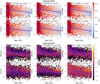 |
Fig. A.1. [s/α] abundance ratios versus age for GALAH. The purple line shows the median abundance per age bin, and the error bar represents a one sigma deviation from the median, as in Fig. 12 but now colour-coded by temperature (upper panels) and metallicity (lower panels). |
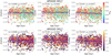 |
Fig. A.2. [s/α] abundance ratios versus age for APOGEE. The purple line shows the median abundance per age bin, and the error bar represents a one sigma deviation from the median, as in Fig. 13 but now colour-coded by temperature (upper panels) and metallicity (lower panels). |
Appendix B: APOGEE DR17 abundances
In this section we investigate the abundance uncertainties and the different stellar synthesis approaches used by the ASPCAP APOGEE DR17 pipeline (García Pérez et al. 2016; Jönsson et al. 2020). Since the ASPCAP pipeline is primarily focussed on and optimised for giant stars, we want to investigate how reliable the abundances used in this work are for the MSTO-SGB stars. We only show figures for the MSTO-SGB regime between temperatures of 5000 K and 6000 K and cleaned by: SNREV > 70, ASPCAP_CHI2 < 25, ASPCAPFLAG = 0, STARFLAG = 0, ELEM_FE_FLAG = 0. We see that the uncertainties show in Fig. B.1 are mostly bellow 0.3 dex for [Mg/Fe],[Si/Fe],[Al/Fe], [Ca/Fe], [Mn/Fe] and [Ni/Fe], statistics is very low for [Co/Fe] and [Ce/Fe], < 3 000. The signal-to-noise, SNREV, is higher for smaller uncertainties, as expected. Still, the quality of the match with synthetic spectral models, ASPCAP_CHI2, is worse for stars with low uncertainty, which might be an effect caused by the temperature range of these stars. Figure B.1 compares the results from two different spectral synthesis codes available on the APOGEE DR17 release. The official release from APOGEE uses a new spectral synthesis code, Synspec (Hubeny & Lanz 2017), that can accommodate the effects of non-LTE for Na, Mg, K, and Ca (Osorio et al. 2020). Although Synspec allows for non-LTE calculations, it uses the assumption of plane parallel geometry, which is not entirely valid for large giant stars. On the other hand, the previous synthesis code used in the APOGEE pipelines, TurboSpectrum (Alvarez & Plez 1998), can use spherical geometry but cannot consider non-LTE effects. Figure B.2 shows non-negligible differences for several elements. We see high spreads for [Na/Fe], [Ti/Fe], and [Cr/Fe], but since those have significant uncertainties, we did not include them in the scientific analysis of this manuscript. Non-LTE effects might be able to explain the differences between the codes, especially for [Na/Fe]. Still, a clear shift is seen for abundances such as [Si/Fe] and [Al/Fe] for temperatures colder than 5500 K, which could be an artefact in the derivation of the abundances. We, therefore, abstain from using [Si/Fe] and [Al/Fe] for temperatures cooler than 5500. [Ce/Fe] shows no concerning differences between the two spectral synthesis codes.
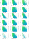 |
Fig. B.1. Abundance uncertainty versus signal-to-noise ratio (SNREV) for each chemical species published in APOGEE DR17. |
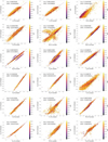 |
Fig. B.2. Comparison between turbospec and Synspec APOGEE DR17. |
Appendix C: Additional t-SNE analysis
In this appendix we add some additional illustrative plots to the combined t-SNE + HDBSCAN analysis performed in Sect. 6 for each of the three SGB samples (GALAH, APOGEE, LAMOST).
In principle, there are a number of hyperparameters both in t-SNE and in the HDBSCAN methods that need to be chosen wisely. Apart from those, the main important choice for our work is the set of input parameters and the selection cuts. We optimised the number of input chemical abundances such that as many chemical elements as possible are used without significantly diminishing the total number of stars with useful abundances. Since t-SNE cannot treat missing data, all chosen chemical abundances have to be mutually available for each star in the final dataset.
Secondly, we needed to choose a sensible configuration of hyperparameters both for t-SNE and HDBSCAN for each survey. In Figs. C.1 through C.6 we show a few plots to explain the robustness of the groupings found when using the unsupervised machine learning technique, t-SNE (Hinton & Roweis 2003; van der Maaten & Hinton 2008), in Sect. 6. We have experience with the ‘perplexity’ and the ‘random_state’ parameter to find the optimal t-SNE projection. The perplexity controls the number of nearest neighbours, while the random state only influences the local minima of the cost functions and therefore has a minor impact on the final projection. The random initialisation factor (random_state) plays a crucial role in validating the robustness of groupings in t-SNE space. We want to ensure that the groups we identify are stable against random variations. The results from Figs. C.3, C.1, and C.5 demonstrate that the young α-rich, thick disk, and thin disk stars remain tightly grouped together in the t-SNE space for different random_state choices, even when the perplexities vary widely. This suggests that the groupings are robust and not affected by random variations.
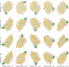 |
Fig. C.1. t-SNE projection for the GALAH DR3 SGB sample for different perplexity and random state values. The colours indicate the original groups we found previously and which are represented in Fig. 15. |
However, the GALAH dataset exhibits less robustness as the cyan and purple marked groups of stars do not remain together in the t-SNE space across different random_states and perplexities. On the other hand, the high-Ba stars marked in red and high-Ni peculiar stars marked in royal blue remain consistently grouped together in the t-SNE space when different t-SNE parameters are used. These findings suggest that care must be taken when interpreting the results we found as cyan and purple groupings since their validity is less robust across changes in t-SNEs parameters.
After testing several perplexity values, we selected the one that best accentuates the separation between the two largest populations in the solar neighbourhood, namely the thick and thin disks. By choosing the optimal perplexity value, we were able to obtain a clear separation in a multi-dimensional chemical analysis. Our results show that mostly high values of perplexity are better suited for our datasets, especially for APOGEE and GALAH. For LAMOST high perplexity values do not improve the visualisation of the different populations.
We similarly chose the final HDBSCAN hyperparameters, first fixing a t-SNE configuration that visually shows two or more overdensities and then we experienced with different values for min_cluster_size, which controls the minimum size of the groupings, the min_samples, which controls how conservative the clustering is and the cluster_selection_epsilon, which controls the separation distance between the groups, for more information on the HDBSCAN parameters we recommend the reader to the following page7. By testing HDBSCAN hyperparameters with a fixed t-SNE configuration and vice versa, we settled for the values described in Table 5, which optimally separates the chemical thin and thick disks and also find other structures. The chrono-chemical groups found are also reproducible for many other hyperparameter combinations, which supports the groupings’ robustness.
In Figs. C.2, C.4, and C.6 we show the t-SNE projections colour-coded by different parameters. Since this method could project false groups due to artefacts in the chemical abundances derivation. In all cases, the projected t-SNE has no clear dependence on signal-to-noise, which controls the quality of the spectra. For LAMOST and GALAH there is also no clear connection between the projected density and the surface gravity, while for APOGEE Fig. C.4 shows that low log g is preferentially at the bottom left of the map. The temperature and metallicity seem to influence the projections for all surveys. The metallicity is information given to the t-SNE method in the form of abundance ratios; therefore, we expect to find different clumps of metallicity across the new t-SNE dimension. This might also influence the temperature distribution since stars with a certain metallicity are easier to detect at certain temperatures.
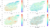 |
Fig. C.2. t-SNE projection for GALAH DR3 SGB data colour-coded by Teff, log g, metallicity, and signal to noise. |
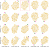 |
Fig. C.3. t-SNE projection for the APOGEE DR17 SGB sample using different values of perplexity and random state. We use the HDBSCAN method for each panel on top of the t-SNE projection. The colours indicate the original groups we found previously and which are represented in Fig. 14. |
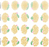 |
Fig. C.5. t-SNE projection for the LAMOST DR7 SGB sample using different values of perplexity and random state. We use the HDBSCAN method for each panel on top of the t-SNE projection. The colours indicate the original groups we found previously and which are represented in Fig. 16. |
C.1. t-SNE uncertainties
Manifold learning algorithms cannot treat observational uncertainties and also do not provide uncertainties associated with the produced mapping. They merely provide a projection of a high-dimensional dataset into a lower-dimensional space. We reinforce that the primary method behind our analysis is the dimensionality reduction technique, collapsing the multiple chemical-age spaces into a two-dimensional visualisation. We then used HDBSCAN to avoid delineating the overdensities by eye. Throughout the analysis, we have already had a critical validation of the method: We recover the thin disk, thick disk and young-α-rich in three completely different surveys. Limberg et al. (2021) and Ou et al. (2023) used HDBSCAN alone to find groupings in kinematics space, and Monte-Carlo experiments were able to assign a certain probability of pertinence to the clusters. In our case, this is much more difficult since each random re-sampling of our data will result in a new projection space for t-SNE. Here we do a small exercise to test the robustness of the groups found by t-SNE+HDBSCAN. As in Anders et al. (2018, see their Fig. 5), we introduce noise to the data in a Monte-Carlo experiment test. We sampled 20 random abundances and ages for each star using a Gaussian distribution centred in the abundance and age using its uncertainties as standard deviation. We then ran t-SNE on this increased random sample. In Fig. C.7 we show the result of the new t-SNE projection in this ‘noisy’ data as grey points and with the original tagged groups in their respective colours (see Figs. 16, 14, and 15) versus the original t-SNE map. For the thick, thin disk and young α-rich groups, the overdensities are preserved even with the introduced noise in all three surveys. For GALAH, some populations get dispersed by the experiment, especially the young peculiar navy blue group, while the outer disk cyan is in the middle of the thin disk group. The high barium stars are an overdensity that remains visibly separable from the thin disk main cloud. We want to stress also that adding noise to the data may artificially blur real signals. Despite the significance of the cyan, purple, and navy blue groups being less robust, these findings are still an essential first step to the investigation of these populations in the Milky Way since they present some interesting features as the peaked age of the cyan group.
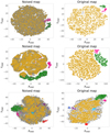 |
Fig. C.7. t-SNE projections of noised data (produced by randomly adding Gaussian uncertainties to the abundances and ages of each star) versus original data. Top row: APOGEE. Middle row: LAMOST. Bottom row: GALAH. |
All Tables
Mean relative error or uncertainty per StarHorse output parameter per spectroscopic survey.
All Figures
|
Fig. 1. Sky distribution of all public spectroscopic surveys for which we derive StarHorse parameters. |
| In the text | |
|
Fig. 2. Uncertainty distributions for StarHorse results. Left and middle panels: probability density functions of StarHorse output parameters and their respective uncertainties. The distributions are shown for each spectroscopic survey separately, as indicated in the legend. The upper panels, which show the distance and extinction, have their y-axis in logarithm scale to show the extent to larger values. Right panels: median trend of the dependence of each parameter with its associated uncertainty. |
| In the text | |
|
Fig. 3. Galactic distribution of all spectroscopic surveys for which we present StarHorse results in this paper. The grey background density shows the star counts for all surveys combined, while the coloured bands trace the region between iso-contours of 25 000 and 15 000 stars per pixel for each survey. To guide the eye, grey circles are placed in multiples of 5 kpc around the Galactic centre in the left panel. The approximate location and extent of the Galactic bar is indicated by the black ellipse (minor axis = 2 kpc; major axis = 8 kpc; inclination = 25°), and the solar position is marked by the dashed lines. Left panel: cartesian XY projection. Right panel: cylindrical RZ projection. |
| In the text | |
|
Fig. 4. Consistency of StarHorse input and output parameters. Top panels: median of the relative discrepancy between input parameters and StarHorse output parameters for each survey. Bottom panels: median of the dependence between input uncertainties versus input parameters. |
| In the text | |
|
Fig. 5. StarHorse Kiel diagram for the samples studied in this work. The grey dots in the background of each panel show all the stars in the respective survey, while the colour-coded histograms highlight the MSTO+SGB regime for which we deliver StarHorse ages. The dashed lines delimit the SGB, for which the computed ages are most precise. PARSEC isochrones are overplotted in red for three different metallicities, as indicated in the lower-right corner of the figure. For each metallicity, four different ages are shown: 1, 4, 7, and 10 Gyr. |
| In the text | |
|
Fig. 6. Distributions of ages, masses, distances, and their uncertainties for the MSTO+SGB samples. The y-axis shows the probability density. All histograms are normalised so that the area under the histogram integrates to 1. The right panels show the mean age uncertainty per bin of age, mass, and distance for each survey. |
| In the text | |
|
Fig. 7. Galactocentric X and Z projection of MSTO+SGB samples colour-coded by StarHorse ages. The colour bar is in power law scale with γ = 0.7. |
| In the text | |
|
Fig. 8. Comparison of our MSTO+SGB age estimates with OC ages from Cantat-Gaudin et al. (2020). In each panel, grey dots are individual OC member MSTO stars (membership probability > 95%), colour-coded by their posterior age uncertainty. For OCs that contain more than three MSTO cluster members, the uniform coloured points and error bars indicate the median age and the 1σ quantiles. The star symbol indicates the SGB-only sample, which has lower StarHorse uncertainties. The horizontal error bars reflect the 0.2 dex uncertainties quoted by Cantat-Gaudin et al. (2020). The only OC that was observed by all surveys is M 67 (NGC 2682). We do not show comparisons for RAVE and SDSS since there were fewer than five stars in common with the cluster sample. The dashed black line delineates the identity line, while the grey dashed lines correspond to a ±30% deviation. |
| In the text | |
|
Fig. 9. Comparison of our MSTO+SGB age estimates with values from the recent literature. From top left to bottom right: comparison to the LAMOST DR7 ages of Xiang & Rix (2022), the GALAH DR3 ages of Buder et al. (2021), the LAMOST, RAVE, and APOGEE age estimates of Mints (2020), and the ages calculated by Kordopatis et al. (2023) for the Gaia RVS sample. In each panel we show the number density of stars, and the magenta points indicate the median trends. The global spread for each comparison is shown as the mean absolute deviation (mad) and the global shift as the mean deviation (mad). |
| In the text | |
|
Fig. 10. [α/Fe] versus [Fe/H] distributions for the MSTO+SGB samples of the analysed surveys. Left: density distributions relative to the maximum count in each survey. Right: same, but coloured by the mean age per pixel. |
| In the text | |
|
Fig. 11. [α/Fe] versus age distribution for the MSTO+SGB samples of each survey. A cleaning per signal to noise and suggested flags was performed. The purple squares show the median trend per bin in [α/Fe], while the error bars show its one σ deviation. We only display the surveys that have mean statistical uncertainty in age < 20% according to Table 2 (no RAVE or Gaia RVS). We also performed a cleaning of flags in the [α/Fe] determination from each survey. |
| In the text | |
|
Fig. 12. [s/α] abundance ratios versus age for GALAH. The purple line shows the median abundance per age bin, and the error bar represents a one sigma deviation from the median. |
| In the text | |
|
Fig. 13. [s/α] abundance ratios versus age for APOGEE. The purple line shows the median abundance per age bin, and the error bar represents a one sigma deviation from the median. |
| In the text | |
|
Fig. 14. General results of the t-SNE+HDBSCAN application. Upper-left panel: t-SNE projection for SGB stars in APOGEE DR17. Colours correspond to different groups found by t-SNE+HDBSCAN on the data. Lower-left and middle panels: abundance ratios of α elements to those of the iron group plotted against metallicity using the same colours for each identified group. Right panels (from top to bottom: i): (i) cumulative age distribution for each group; (ii) mean azimuthal velocity (left y-axis and square symbol) and mean dispersion in azimuthal velocity (right y-axis and star symbol) for each group as a function of age; (iii) mean vertical velocity (left y-axis and square symbol) and mean dispersion in vertical velocity (right y-axis and star symbol) for each group as a function of age; (iv) mean metallicity (left y-axis and square symbol) and mean dispersion in metallicity (right y-axis and star symbol) for each group as a function of age. The error bars in the right panels represent the 95% confidence interval of a bootstrap resampling. |
| In the text | |
|
Fig. 15. t-SNE projection for SGB stars in GALAH DR3. Colours correspond to each group found by t-SNE+HDBSCAN from GALAH data. Abundance ratios are also shown, with the same colour coding. Upper panels: cumulative age distribution for each group. Middle panels: mean azimuthal velocity (left axis squares) and mean dispersion in azimuthal velocity (right axis stars) for each group. Lower panels: mean vertical velocity (left axis squares) and mean dispersion in vertical velocity (right axis stars) for each group. The error bars in the right panels represent the 95% confidence interval of a bootstrap resampling. |
| In the text | |
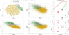 |
Fig. 16. t-SNE projection for SGB stars in LAMOST MRS. Same as Fig. 14 but for LAMOST MRS data. |
| In the text | |
|
Fig. 17. Probability density function of metallicity, age, and [Mg/Fe] for the main populations found in APOGEE, GALAH, and LAMOST with t-SNE HDBSCAN. |
| In the text | |
|
Fig. 18. Age metallicity relations for the thin disk. Upper panels: metallicity versus age for the detected thin-disk component in three surveys. The map shows the mean density per pixel where we have also applied Gaussian smoothing. The dotted red line represents the median metallicity for the given age. Lower panels: heliocentric distance coverage for each sample. |
| In the text | |
|
Fig. 19. Age versus [Mg/Fe] for the young α-rich groups found in APOGEE, GALAH, and LAMOST. The black delineation shows the region that chemical evolutionary models cannot explain, as in Chiappini et al. (2014). |
| In the text | |
|
Fig. A.1. [s/α] abundance ratios versus age for GALAH. The purple line shows the median abundance per age bin, and the error bar represents a one sigma deviation from the median, as in Fig. 12 but now colour-coded by temperature (upper panels) and metallicity (lower panels). |
| In the text | |
|
Fig. A.2. [s/α] abundance ratios versus age for APOGEE. The purple line shows the median abundance per age bin, and the error bar represents a one sigma deviation from the median, as in Fig. 13 but now colour-coded by temperature (upper panels) and metallicity (lower panels). |
| In the text | |
|
Fig. B.1. Abundance uncertainty versus signal-to-noise ratio (SNREV) for each chemical species published in APOGEE DR17. |
| In the text | |
|
Fig. B.2. Comparison between turbospec and Synspec APOGEE DR17. |
| In the text | |
|
Fig. C.1. t-SNE projection for the GALAH DR3 SGB sample for different perplexity and random state values. The colours indicate the original groups we found previously and which are represented in Fig. 15. |
| In the text | |
|
Fig. C.2. t-SNE projection for GALAH DR3 SGB data colour-coded by Teff, log g, metallicity, and signal to noise. |
| In the text | |
|
Fig. C.3. t-SNE projection for the APOGEE DR17 SGB sample using different values of perplexity and random state. We use the HDBSCAN method for each panel on top of the t-SNE projection. The colours indicate the original groups we found previously and which are represented in Fig. 14. |
| In the text | |
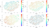 |
Fig. C.4. Same as Fig. C.2 but for the APOGEE DR17 SGB sample. |
| In the text | |
|
Fig. C.5. t-SNE projection for the LAMOST DR7 SGB sample using different values of perplexity and random state. We use the HDBSCAN method for each panel on top of the t-SNE projection. The colours indicate the original groups we found previously and which are represented in Fig. 16. |
| In the text | |
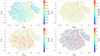 |
Fig. C.6. Same as Fig. C.2 but for the LAMOST DR7 SGB sample. |
| In the text | |
|
Fig. C.7. t-SNE projections of noised data (produced by randomly adding Gaussian uncertainties to the abundances and ages of each star) versus original data. Top row: APOGEE. Middle row: LAMOST. Bottom row: GALAH. |
| In the text | |
Current usage metrics show cumulative count of Article Views (full-text article views including HTML views, PDF and ePub downloads, according to the available data) and Abstracts Views on Vision4Press platform.
Data correspond to usage on the plateform after 2015. The current usage metrics is available 48-96 hours after online publication and is updated daily on week days.
Initial download of the metrics may take a while.